Annals of Physics 343 (2014) 1–15

Contents lists available at ScienceDirect

Annals of Physics

journal homepage: www.elsevier.com/locate/aop

The one and a half monopoles solution of theSU(2) Yang–Mills–Higgs field theoryRosy Teh ∗, Ban-Loong Ng, Khai-Ming WongSchool of Physics, Universiti Sains Malaysia, 11800 USM Penang, Malaysia

h i g h l i g h t s

• This one-half monopole can co-exist with a ’t Hooft–Polyakov monopole.• The magnetic charge of the one-half monopole and one monopole is of opposite sign.• This solution is non-BPS.• The net magnetic charge of the configuration is zero.• This solution upon Cho decomposition is only singular along the negative z-axis.

a r t i c l e i n f o

Article history:Received 11 June 2013Accepted 2 January 2014Available online 9 January 2014

Keywords:SolitonMonopoleYang–Mills–Higgs theory

a b s t r a c t

Recently we have reported on the existence of finite energy SU(2)Yang–Mills–Higgs particle of one-half topological charge. In thispaper, we show that this one-half monopole can co-exist witha ’t Hooft–Polyakov monopole. The magnetic charge of the one-half monopole is of opposite sign to the magnetic charge of the’t Hooft–Polyakov monopole. However the net magnetic charge ofthe configuration is zero due to the presence of a semi-infiniteDiracstring along the positive z-axis that carries the other half of themagnetic monopole charge. The solution possesses gauge poten-tials that are singular along the z-axis, elsewhere they are regular.The total energy is found to increase with the strength of the Higgsfield self-coupling constant λ. However the dipole separation andthemagnetic dipole moment decrease with λ. This solution is non-BPS even in the BPS limit when the Higgs self-coupling constantvanishes.

© 2014 Elsevier Inc. All rights reserved.

∗ Corresponding author.E-mail address: rosyteh@usm.my (R. Teh).

0003-4916/$ – see front matter© 2014 Elsevier Inc. All rights reserved.http://dx.doi.org/10.1016/j.aop.2014.01.003

2 R. Teh et al. / Annals of Physics 343 (2014) 1–15

1. Introduction

The SU(2) Yang–Mills–Higgs (YMH) field theory in 3 + 1 dimensions, with the Higgs field inthe adjoint representation is one of the simplest non-Abelian gauge field theory to investigate andstudy. In spite of its simplicity, this gauge field theory possesses a large variety of monopoles andantimonopoles configurations that have been found and studied bymany physicists since mid-1970s.These monopole solution belongs to the category of solutions which are invariant under a U(1)subgroup of the local SU(2) gauge group. Most of the solutions discussed are numerical solutionsespecially when the Higgs field potential is nonvanishing. So far to our knowledge, no exactmonopolesolutions has been found when the Higgs field self-coupling constant, λ, is nonvanishing. Even the ’tHooft–Polyakovmonopole solution [1] which is the first finite energymonopole solution is numericalwhen λ = 0 [2].

From the mid-1970s through the 1980s, many interesting monopole solutions have been foundand studied. However the exact solutions found are only for the case when the Higgs potential van-ishes and they are Bogomol’nyi–Prasad–Sommerfield (BPS) solutions [3] that satisfied the first or-der partial differential Bogomol’nyi equation. Hence these exact solutions [3,4] are actually self-dualsolutions of the Yang–Mills (YM) field theory [5]. Other exact solutions found are the A–M–A (anti-monopole–monopole–antimonopole) and vortex ring solutions and various other mirror symmet-ric monopole configurations [6]. Numerical BPS monopole solutions with no rotational symmetryhave also been discussed [7]. Other numerical finite energy monopole solutions include the MAP(monopole–antimonopole-pair), MAC (monopole–antimonopole-chain), and vortex ring solutions[8].

The only spherically symmetric monopole solution is the unit magnetic charge ’t Hooft–Polyakovmonopole solution [1]. Finite energy monopole configurations with magnetic charges greater thanunity [4] cannot possess spherical symmetry [9]. We have also notice through the work of others andour work that there are no spherically symmetric monopole solution when there are more than onepoles in the configuration even though the net magnetic monopole charge is zero or unity. Howeverthey can possess axial symmetry.

Most of these monopole solutions reported so far are of integer topological monopole charges.There are very limited work on configurations with one-half magnetic monopole charge particle.Report on one-halfmonopoles in the Yang–Mills (YM) theory include thework ofHarikumar et al. [10].They demonstrated the existence of generic smooth YM potentials of one-half monopoles. Howeverno exact or numerical solutions have been given. Exact one-halfmonopole axially symmetric solutionsand one-half monopole mirror symmetric solutions with Dirac-like string have also been discussed inRef. [11]. However these configurations do not possess finite energies.

Recently we have reported on the existence of finite energy SU(2) YMH particle of one-halftopological charge [12]. Unlike the ’t Hooft–Polyakov monopole, this one-half monopole possessesnonvanishing magnetic dipole moment as well as angular momentum when electric charge isintroduced into the solution. Hence the electrically charged one-half monopole possesses rotationalkinetic energy and it is able to rotate in the presence of an externalmagnetic field [13]. Furtherwork onthis one-half monopole shows that it can co-exist with a ’t Hooft–Polyakov monopole. The magneticcharge of the one-half monopole and one monopole are of opposite sign. However the net magneticcharge of the configuration is zero due to the presence of a semi-infinite Dirac string along the positivez-axis that carries the other half of themagnetic monopole charge. This new solution possesses gaugepotentials that are singular along the z-axis, elsewhere they are regular.

Similar to the one-half monopole configuration, the total energy of this new solution increaseswith the strength of the Higgs field self-coupling constant λ. However the dipole separation and themagnetic dipole moment decrease with λ. This solution is non-BPS even in the BPS limit when theHiggs self-coupling constant vanishes.

We briefly review the SU(2) YMH field theory in Section 2. The magnetic ansatz used in obtainingthe one and a half monopoles solution and some of its basic properties are presented in Section 3. Thenumerical finite energy, one and a half magnetic monopoles solution and some of its properties arepresented and discussed in Section 4. We end with some comments in Section 5.

R. Teh et al. / Annals of Physics 343 (2014) 1–15 3

2. The SU(2) YMH Theory

The SU(2) YMH Lagrangian in 3 + 1 dimensions with nonvanishing Higgs potential is given by

L = −14F aµνF

aµν−

12DµΦaDµΦa

−14λ

ΦaΦa

−µ2

λ

2

. (1)

Here the Higgs field mass is µ and the strength of the Higgs potential is λ which are constants. Thevacuum expectation value of the Higgs field is ξ = µ/

√λ. The Lagrangian (1) is gauge invariant under

the set of independent local SU(2) transformations at each space–time point. The covariant derivativeof the Higgs field and the gauge field strength tensor are given respectively by

DµΦa= ∂µΦ

a+ gϵabcAb

µΦc,

F aµν = ∂µAa

ν − ∂νAaµ + gϵabcAb

µAcν, (2)

where g is the gauge field coupling constant. The metric used is gµν = (− + ++). The SU(2) internalgroup indices a, b, c = 1, 2, 3 and the space–time indices are µ, ν, α = 0, 1, 2, and 3 in Minkowskispace. The equations of motion that follow from the Lagrangian (1) are

DµF aµν = ∂µF a

µν + gϵabcAbµF cµν = gϵabcΦbDνΦc,

DµDµΦa= λΦa(ΦbΦb

− ξ 2). (3)

In the limit of vanishingµ and λ, the Higgs potential vanishes and self-dual solutions can be obtainedby solving the first order partial differential Bogomol’nyi equation,

Bai ± DiΦ

a= 0, where Ba

i = −12ϵijkF a

jk. (4)

The electromagnetic field tensor proposed by ’t Hooft [1] upon symmetry breaking is

Fµν = ΦaF aµν −

1gϵabcΦaDµΦbDνΦc

= Gµν + Hµν, (5)

where Gµν = ∂µAν − ∂νAµ and Hµν = −1gϵabcΦa∂µΦ

b∂νΦc, (6)

are the gauge part and the Higgs part of the electromagnetic field respectively. Here Aµ = ΦaAaµ,

the Higgs unit vector, Φa= Φa/|Φ|, and the Higgs field magnitude |Φ| =

√ΦaΦa. Hence the

decomposed magnetic field is

Bi = −12ϵijkFjk = BG

i + BHi , (7)

where BGi and BH

i are the gauge part andHiggs part of themagnetic field respectively. The netmagneticcharge of the system is

M =14π

∂ iBi d3x =

14π

d2σi Bi. (8)

The topological magnetic current, kµ =18π ϵµνρσ ϵabc ∂

νΦa ∂ρΦb ∂σ Φc , is also the topologicalcurrent density of the system [14]. Hence the corresponding conserved topological magnetic chargeis

MH =1g

d3x k0 =

18πg

ϵijkϵ

abc∂i

Φa∂jΦ

b∂kΦcd3x

=18π

d2σi

1gϵijkϵ

abcΦa∂jΦb∂kΦ

c

=14π

d2σi BH

i . (9)

4 R. Teh et al. / Annals of Physics 343 (2014) 1–15

The magnetic charge MH is the total magnetic charge of the system if and only if the gauge field isnon singular [15]. If the gauge field is singular and carries Dirac string monopoles MG, then the totalmagnetic charge of the system is

M = MG + MH , where

MG = −18π

d2σiϵijk

∂jAk − ∂kAj

=

14π

d2σi BG

i . (10)

In the electrically neutral BPS limit when the Higgs potential vanishes, the energy is a mini-mum, [14]

Emin = ∓

∂i(Ba

iΦa) d3x +

12(Ba

i ± DiΦa)2 d3x

= ∓

∂i(Ba

iΦa) d3x =

4πξg

MH , (11)

when the vacuum expectation value of the Higgs field is nonzero. Hence the minimum dimensionlesstotal energy isMH .

For a non-BPS solution, its energy must be greater than that given by Eq. (11). The dimensionlessvalue is given by

E =g

8πξ

Bai B

ai + DiΦ

aDiΦa+λ

2(ΦaΦa

− ξ 2)2

d3x ≥ MH . (12)

Since the one and ahalfmonopoles solution is singular along the z-axis, it is useful to define aweightedenergy density, E = the dimensionless energy density × 2πr2 sin θ .

The gauge potential Aaµ and the Higgs field Φa can be gauge transformed by local SU(2) gauge

transformations which can be written in the 2 × 2 matrix form, [5]

ω(x) = exp

i2σana(x)f (x)

= cos

12f (x)

+ iσana(x) sin

12f (x)

, (13)

where na(x) is a unit vector and σa is the Pauli matrix. The transformed gauge potential and Higgs fieldthen takes the form,

A′aµ = cos fAa

µ + sin f ϵabcAbµn

c+ 2 sin2 f

2na(nbAb

µ)

+

na∂µf + sin f ∂µna

+ 2 sin2 f2ϵabc(∂µnb)nc

(14)

Φ ′a= cos fΦa

+ sin f ϵabcΦbnc+ 2 sin2 f

2na(nbΦb). (15)

3. The construction of the solution

3.1. The magnetic ansatz

The magnetic ansatz [8] is given by

gAai = −

1rψ1(r, θ)na

φ θi +1

r sin θP1(r, θ)na

θ φi +1rR1(r, θ)na

φ ri −1

r sin θP2(r, θ)na

r φi,

gAa0 = 0, gΦa

= Φ1(r, θ) nar + Φ2(r, θ)na

θ , (16)

where P1(r, θ) = sin θ ψ2(r, θ) and P2(r, θ) = sin θ R2(r, θ). The spatial spherical coordinateorthonormal unit vectors are, ri = sin θ cosφ δi1 + sin θ sinφ δi2 + cos θ δi3, θi = cos θ cosφ δi1

R. Teh et al. / Annals of Physics 343 (2014) 1–15 5

+ cos θ sinφ δi2 − sin θ δi3, φi = − sinφ δi1 + cosφ δi2, and the isospin coordinate orthonormal unitvectors are

nar = sin θ cos nφ δa1 + sin θ sin nφ δa2 + cos θ δa3,

naθ = cos θ cos nφ δa1 + cos θ sin nφ δa2 − sin θ δa3,

naφ = − sin nφ δa1 + cos nφ δa2; where n ≥ 1. (17)

The φ-winding number n is a natural number. The θ-winding number m [8] in the ansatz (16) ism = 1. In our work here on one and a half monopoles we take n = 1. The magnetic ansatz (16) isform invariant under the gauge transformation, ω = exp

i2σ

anaφ f (r, θ)

and the transformed gauge

potential and Higgs field take the form,

gA′ai = −

1r{ψ1 − ∂θ f }na

φ θi +1

r sin θ{P1 cos f + P2 sin f + n[sin θ − sin(f + θ)]} na

θ φi

+1r{R1 + r∂r f }na

φ ri −1

r sin θ{P2 cos f − P1 sin f + n[cos θ − cos(f + θ)]} na

r φi,

gA′a0 = 0,

gΦ ′a= (Φ1 cos f + Φ2 sin f ) na

r + (Φ2 cos f − Φ1 sin f )naθ . (18)

The general Higgs fields in the spherical and the rectangular coordinate systems are

gΦa= Φ1(x) na

r + Φ2(x)naθ + Φ3(x)na

φ

= Φ1(x) δa1 + Φ2(x) δa2 + Φ3(x) δa3, (19)

respectively, where

Φ1 = sin θ cos nφ Φ1 + cos θ cos nφ Φ2 − sin nφ Φ3 = |Φ| sinα cosβ

Φ2 = sin θ sin nφ Φ1 + cos θ sin nφ Φ2 + cos nφ Φ3 = |Φ| sinα sinβ

Φ3 = cos θ Φ1 − sin θ Φ2 = |Φ| cosα. (20)

The axially symmetric Higgs unit vector in the rectangular coordinate system is

Φa= sinα cosβ δa1 + sinα sinβ δa2 + cosα δa3, (21)

where, cosα = h1(r, θ) cos θ − h2(r, θ) sin θ, β = nφ, (22)

and h1(r, θ) =Φ1

|Φ|, h2(r, θ) =

Φ2

|Φ|.

From Eqs. (21) and (22), the Higgs field (16) and the gauge transformed Higgs field (18) can bewrittenin terms of α as

Φa= |Φ(r, θ)|(cos(α − θ) na

r + sin(α − θ)naθ ),

Φ ′a= |Φ(r, θ)|(cos(α′

− θ) nar + sin(α′

− θ)naθ ), (23)

where α′= α − f .

Similarly the Higgs part of the ’t Hooft magnetic field (7) can be reduced to

gBHi = −nϵijk∂ j cosα∂kφ. (24)

The gauge part of the magnetic field (7) can be written in similar form

gBGi = −nϵijk∂j cos κ ∂kφ, (25)

where, cos κ =1n(h2(r, θ)P1 − h1(r, θ)P2) .

Hence the ’t Hooft’s magnetic field which is the sum of the Higgs part (24) and the gauge part (25) isgiven by

gBi = −nϵijk∂j(cosα + cos κ) ∂kφ = −ϵijk∂jAk, (26)

6 R. Teh et al. / Annals of Physics 343 (2014) 1–15

where Ai is the ’t Hooft’s gauge potential. The magnetic field lines of the configuration can be plottedby drawing the contour lines of (cosα+cos κ) = constant on the vertical planeφ = 0. The orientationof the magnetic field can also be plotted by using the vector plot of the magnetic field unit vector,

Bi =−∂θ (cosα + cos κ)ri + r∂r(cosα + cos κ)θi[r∂r(cosα + cos κ)]2 + [∂θ (cosα + cos κ)]2

. (27)

We can also evaluate numerically the different magnetic charges at different distances r from theorigin by the following definitions,

M{UH} = −12g

{cosα + cos κ}|θ= 1

2π

θ=0,r , M{LH} = −12g

{cosα + cos κ}|θ=πθ= 1

2π,r,

MG = −12g

{cos κ}|θ=πθ=0,r , MH = −12g

{cosα}|θ=πθ=0,r ,

M = −12g

{cosα + cos κ}|θ=πθ=0,r , (28)

where M{UH} and M{LH} are the magnetic charges covered by the upper and lower hemispheresrespectively at distances r from the origin.

At spatial infinity in the Higgs vacuum, all the non-Abelian components of the gauge potentialvanish and the non-Abelian electromagnetic field tends to

F aµν

r→∞

=

∂µAν − ∂νAµ −

1gϵcdeΦc∂µΦ

d∂νΦeΦa

= FµνΦa, (29)

where Fµν is just the ’t Hooft electromagnetic field. However there is no unique way of representingthe Abelian electromagnetic field in the region of themonopole outside theHiggs vacuumat finite val-ues of r [16]. One proposal was given by ’t Hooft as in Eq. (5). Using the ’t Hooft’s magnetic field, themagnetic charge density vanishes, that is ∂ iBi = 0, when |Φ| = 0. However when |Φ| = 0, ∂ iBi = 0and the magnetic charges are located at these points. Hence with ’t Hooft’s definition of the elec-tromagnetic field, the magnetic charges are discrete and reside at the point zeros of the Higgs field.Since this definition gives a discretemagnetic charge at a particular point, there is nomagnetic chargedistribution over space.

Another proposal which is less singular was given by Bogomol’nyi [3] and Faddeev [17], where themagnetic and electric fields are given respectively by

Bi = Bai

Φa

ξ

, Ei = Ea

i

Φa

ξ

. (30)

From Eq. (8), and using the definition for the Abelianmagnetic field (30) given by Bogomol’nyi [3] andFaddeev [16], we can write

M =14π

∂ iBi d3x =

M dθ dr, where M =

12r2 sin θ{∂ iBi}, (31)

is the weighted magnetic charge density. With this definition of the electromagnetic field (30), therewill be a magnetic charge density distribution contributed by the non-Abelian components of thegauge field in the finite r region. A 3D surface plot of the magnetic charge density distribution will beuseful in determining the sign of the magnetic charge of the solutions. In the Higgs vacuum at spatialinfinity, both definitions of the electromagnetic field (5) and (30) become similar.

R. Teh et al. / Annals of Physics 343 (2014) 1–15 7

3.2. The exact asymptotic solutions

The gauge transformation, ω = exp i2σ

anaφ f1(r, θ)

, when applied on to the solution,

gAa0, gAa

i = A(r, θ)δa3φi, gΦa= ξδa3, A(r, θ) =

a cos θ + b − 1r sin θ

, (32)

where, a, b are constants, will rotate the isospin direction, δa3 , into the magnetic ansatz (16) and thetransformed gauge potentials and Higgs field then take the form,

gA′ai = −

1r{−∂θ f1(r, θ)}na

φ θi +1r{∂r f1(r, θ)}na

φ ri

+n

r sin θ{sin θ − sin(f1(r, θ)+ θ)[1 + rA(r, θ) sin θ ]} na

θ φi

−n

r sin θ{cos θ − cos(f1(r, θ)+ θ)[1 + rA(r, θ) sin θ ]} na

r φi,

gA′a0 = 0,

gΦ ′a= ξ{cos(f1(r, θ)+ θ) na

r − sin(f1(r, θ)+ θ)naθ }. (33)

We also note that the angle α = −f1(r, θ). Hence

cosα = cos f1(r, θ), cos κ = − cos f1(r, θ)+ {1 + r sin θA(r, θ)} , (34)

and the ’t Hooft gauge potential and net magnetic field of the monopole configuration are given by

Ai =

a cos θ + b

r sin θ

φi, gBi = −ϵijk∂j{1 + r sin θA(r, θ)}∂kφ =

nar2

ri, (35)

respectively.The one and a half monopoles solution is obtained by substituting f1(r, θ) = −

32θ, a = b =

12 , and

n = 1 into Eq. (33). The profile functions of the gauge potentials and Higgs field are given by,

ψ1 =32, P1 = sin θ +

12sin

12θ(1 + cos θ),

R1 = 0, P2 = cos θ −12cos

12θ(1 + cos θ),

Φ1 = ξ cos12θ, Φ2 = ξ sin

12θ, (36)

and the ’t Hooft gauge potential and Higgs part of the magnetic field of the monopole configurationare given by

Ai =

cos θ + 12r sin θ

φi, gBH

i =

32 sin

32θ

sin θ

rir2, (37)

respectively. Hence the solution possesses ’t Hooft’s gauge potential (37) which is singular along thepositive z-axis, the Higgs part of the magnetic field which is singular along the negative z-axis, anda net topological magnetic charge of 1

2g at r = 0. The non-Abelian magnetic field, gBai =

ri2r2Φa, is

spherically symmetrical, radial in direction in real space and pointing along the Higgs field directionin isospin space. However the net ’t Hooft’s magnetic field is given by

gBi =ri2r2

− 2πδ(x1)δ(x2)θ(x3)δ3i , (38)

when the Dirac string in the gauge potentials, Ai, is taken into consideration [18]. This one and ahalf monopoles solution therefore carry a net positive one-half magnetic monopole charge and a

8 R. Teh et al. / Annals of Physics 343 (2014) 1–15

semi-infinite Dirac string of flux, 2πg , going into the origin. Hence the net magnetic charge of the

configuration is zero.The topological magnetic charge (9), or the magnetic charge carried by the Higgs field at r infinity

can be evaluated to be

MH = −12g

cosα|θ=πθ=0,r→∞

= −12g

cos

32θ

θ= 23π

θ=0+ cos

32θ

θ=πθ= 2

3π

= (+1)+

−

12

= +

12,

when the gauge coupling constant g = 1. Similar to the one-half monopole configuration [9], the nettopological magnetic charge of the one and a half monopoles solution is positive one-half magneticmonopole charge which is the sum of a positive unit magnetic monopole charge and a negative one-half magnetic monopole charge.

3.3. The numerical calculations

The numerical one and a half monopoles solution can be constructed by making use of theexact monopole solution (36) as asymptotic solution at large distances and by fixing the boundaryconditions for the profile functions (16) along the z-axis and near r = 0. Since the function R2(r, θ) issingular along the z-axis, we choose to perform our numerical analysis with the functions,

P1(r, θ) = ψ2(r, θ) sin θ, P2(r, θ) = R2(r, θ) sin θ. (39)

Near the origin, r = 0, we have the common trivial vacuum solution for the one and a halfmonopoles solution. The asymptotic solution and boundary conditions at small distances that willgive rise to finite energy solutions are

ψ1 = P1 = R1 = P2 = 0, Φ1 = ξ0 cos θ, Φ2 = −ξ0 sin θ, (40)

sin θΦ1(0, θ)+ cos θΦ2(0, θ) = 0,

∂r(cos θΦ1(r, θ)− sin θΦ2(r, θ))|r=0 = 0. (41)

The boundary conditions imposed along the positive z-axis for the profile functions (16) of thesolutions are

∂θΦ1(r, θ)|θ=0 = 0, Φ2(r, 0) = 0, ∂θψ1(r, θ)|θ=0 = 0,

R1(r, 0) = 0, P1(r, 0) = 0, ∂θP2(r, θ)|θ=0 = 0, (42)

and along the negative z-axis, the boundary conditions imposed are

Φ1(r, π) = 0, ∂θΦ2(r, θ)|θ=π = 0, ∂θψ1(r, θ)|θ=π = 0,

R1(r, π) = 0, P1(r, π) = 0, ∂θP2(r, θ)|θ=π = 0. (43)

The numerical one and a half monopoles solution connecting the asymptotic solutions (36) at largedistances to the trivial vacuum solution (40) at small distances and subjected to the boundaryconditions (41) near r = 0 and the boundary conditions (42)–(43) along the z-axis, together withthe gauge fixing condition

r∂rR1 − ∂θψ1 = 0, (44)

are solved using the Maple and MATLAB software [19].The second order equations of motion (3) which are reduced to six partial differential equations

with the ansatz (16) are then transformed into a system of nonlinear equations using the finitedifference approximation. The numerical calculations are performed with the system of nonlinearequations been discretized on a non-equidistant grid of size 70× 60 covering the integration regions

R. Teh et al. / Annals of Physics 343 (2014) 1–15 9

0 ≤ x ≤ 1 and 0 ≤ θ ≤ π . Here x =r

r+1 is the finite interval compactified coordinate. The partialderivative with respect to the radial coordinate is then replaced accordingly by ∂r → (1 − x)2∂x and∂2

∂r2→ (1 − x)4 ∂

2

∂ x2− 2(1 − x)3 ∂

∂ x . We first used Maple to find the Jacobian sparsity pattern for thesystem of nonlinear equations. After thatwe provide this information toMATLAB to run the numericalcomputation. The system of nonlinear equations are then solved numerically using the trust-region-reflective algorithm by providing the solver with good initial guess. The second order equations ofmotion Eq. (3) are solved when the φ-winding number n = 1, with nonzero expectation value ξ = 1,gauge coupling constant g = 1, and when the Higgs self-coupling constant 0 ≤ λ ≤ 12. In ourcalculations, there are two kinds of error, the first inherited from the finite difference approximationof the functions,which is of the order of 10−4. The second comes from the linearization of the nonlinearequations for MATLAB to solve numerically; the remainder or approximation error is of the order of10−6. Hence the overall error estimate is 10−4.

4. The numerical results

The profile functions obtained for the numerical one and a half monopoles solution, ψ1, P1, R1,

P2,Φ1, andΦ2, are all regular functions of r and θ . However the function R2 =P2

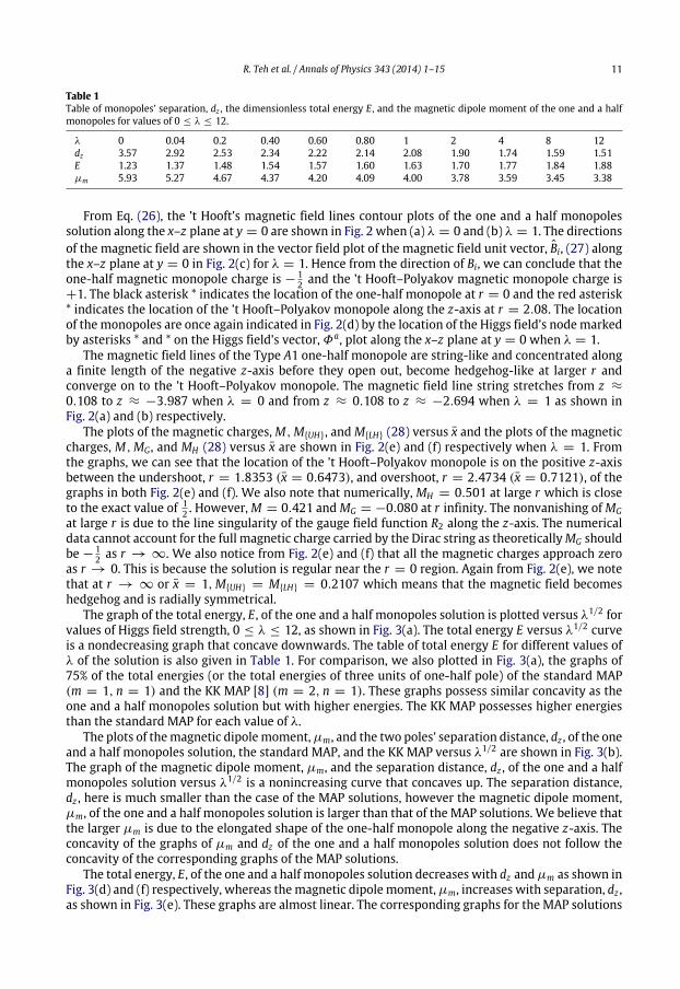
sin θ possesses a stringsingularity along the z-axis as the function P2 = 0 along the z-axis except at r = 0 and z = +∞. InFig. 1(a), the 3D surface and contour plots of the modulus of the Higgs field functions |Φ| of the oneand a half monopoles solution along the x–z plane at y = 0 when λ = 1, show that there are twopoint zeros of the Higgs field modulus along the z-axis at r = 0 and z = dz = 2.08. Hence the one-half monopole and the one-monopole are located at these points where the Higgs field vanishes. Asexpected from the results of the previous paper [12], the shape of the inverted cone for the one-halfmonopole is that of a flatten cone with its half-rounded vertex touching r = 0. The cone is flattenalong the negative z-axis for the Type A one-half monopole. This is in contrast to the inverted coneof the Higgs modulus for the ’t Hooft–Polyakov monopole which is a sharp vertex circular cone withits vertex at z = 2.08, where there is only one zero of |Φ| at r = 0. In the case of the one-halfmonopole there is a double zero of |Φ| at r = 0 along the negative side of the z-axis, for the Type Asolution.

The 3D surface and contour line plots of the weighted energy density E of the one and a halfmonopoles solution along the x–z plane at y = 0 when λ = 1 are shown in Fig. 1(b). In Ref. [12],we found that for the individual Type A1 one-half monopole solution, the weighted energy densitypeak is located at x = ±0.050, and z = −2.860 with peak value of 1.136 while the weightedenergy density peak of the individual ’t Hooft–Polyakov monopole solution has two distinct peakvalues of 0.367 at x = ±1.004 and z = 0. When the Type A1 one-half monopole co-exist with the’t Hooft–Polyakovmonopole, we find that theweighted energy density peak of the one-halfmonopoleis located at z = −2.562 and x = ±0.076 with peak value of 0.998 while the energy density peakof the ’t Hooft–Polyakov monopole solution has two distinct peak values of 0.916 at x = ±0.612and z = 2.256. Hence the shape of the one-half monopole is still that of a rugby ball whereas the’t Hooft–Polyakovmonopole is still shaped like a torus. However the torus now is compressed radiallyalong the x–y plane towards the z-axis.

The 3D surface and contour plots of the weightedmagnetic charge density,M, (31) for the one anda halfmonopoles solution along the x–z plane at y = 0whenλ = 1 are shown in Fig. 1(c).Wenote thatthe negative weighted magnetic charge density is concentrated along the negative z-axis with peakvalue of −0.956 at x = ±0.076 and z = −2.562 and the positive weighted magnetic charge densityis concentrated along the positive z-axis with peak value of 0.828 at x = ±0.612 and z = 2.256.We also note that the weighted magnetic charge density is solely positive for the ’t Hooft–Polyakovmonopole and solely negative for the one-half monopole. For the case of the individual Type A1 one-half monopole, the peak value is 1.081 and located at x = ±0.050 and z = −2.860 whereas for thecase of the individual ’t Hooft–Polyakovmonopole, the peak value is 0.332 and located at x = ±1.004and z = 0 [12]. Hence other than the sign of the weighted magnetic charge density, the weightedmagnetic charge density distribution is similar to the weighted energy density distribution of thesolution.

10 R. Teh et al. / Annals of Physics 343 (2014) 1–15

a

b

c

Fig. 1. The 3D surface and contour plots of (a) the Higgs field modulus, |Φ|, (b) the weighted energy density, E , and (c) theweighted magnetic charge density, M, of the one and a half monopoles solution along the x–z plane at y = 0 when λ = 1.

R. Teh et al. / Annals of Physics 343 (2014) 1–15 11

Table 1Table of monopoles’ separation, dz , the dimensionless total energy E, and the magnetic dipole moment of the one and a halfmonopoles for values of 0 ≤ λ ≤ 12.

λ 0 0.04 0.2 0.40 0.60 0.80 1 2 4 8 12dz 3.57 2.92 2.53 2.34 2.22 2.14 2.08 1.90 1.74 1.59 1.51E 1.23 1.37 1.48 1.54 1.57 1.60 1.63 1.70 1.77 1.84 1.88µm 5.93 5.27 4.67 4.37 4.20 4.09 4.00 3.78 3.59 3.45 3.38

From Eq. (26), the ’t Hooft’s magnetic field lines contour plots of the one and a half monopolessolution along the x–z plane at y = 0 are shown in Fig. 2 when (a) λ = 0 and (b) λ = 1. The directionsof the magnetic field are shown in the vector field plot of the magnetic field unit vector, Bi, (27) alongthe x–z plane at y = 0 in Fig. 2(c) for λ = 1. Hence from the direction of Bi, we can conclude that theone-half magnetic monopole charge is −

12 and the ’t Hooft–Polyakov magnetic monopole charge is

+1. The black asterisk * indicates the location of the one-half monopole at r = 0 and the red asterisk* indicates the location of the ’t Hooft–Polyakov monopole along the z-axis at r = 2.08. The locationof the monopoles are once again indicated in Fig. 2(d) by the location of the Higgs field’s nodemarkedby asterisks * and * on the Higgs field’s vector,Φa, plot along the x–z plane at y = 0 when λ = 1.

The magnetic field lines of the Type A1 one-half monopole are string-like and concentrated alonga finite length of the negative z-axis before they open out, become hedgehog-like at larger r andconverge on to the ’t Hooft–Polyakov monopole. The magnetic field line string stretches from z ≈

0.108 to z ≈ −3.987 when λ = 0 and from z ≈ 0.108 to z ≈ −2.694 when λ = 1 as shown inFig. 2(a) and (b) respectively.

The plots of the magnetic charges,M,M{UH}, andM{LH} (28) versus x and the plots of the magneticcharges, M,MG, and MH (28) versus x are shown in Fig. 2(e) and (f) respectively when λ = 1. Fromthe graphs, we can see that the location of the ’t Hooft–Polyakov monopole is on the positive z-axisbetween the undershoot, r = 1.8353 (x = 0.6473), and overshoot, r = 2.4734 (x = 0.7121), of thegraphs in both Fig. 2(e) and (f). We also note that numerically, MH = 0.501 at large r which is closeto the exact value of 1

2 . However,M = 0.421 andMG = −0.080 at r infinity. The nonvanishing ofMGat large r is due to the line singularity of the gauge field function R2 along the z-axis. The numericaldata cannot account for the full magnetic charge carried by the Dirac string as theoreticallyMG shouldbe −

12 as r → ∞. We also notice from Fig. 2(e) and (f) that all the magnetic charges approach zero

as r → 0. This is because the solution is regular near the r = 0 region. Again from Fig. 2(e), we notethat at r → ∞ or x = 1,M{UH} = M{LH} = 0.2107 which means that the magnetic field becomeshedgehog and is radially symmetrical.

The graph of the total energy, E, of the one and a half monopoles solution is plotted versus λ1/2 forvalues of Higgs field strength, 0 ≤ λ ≤ 12, as shown in Fig. 3(a). The total energy E versus λ1/2 curveis a nondecreasing graph that concave downwards. The table of total energy E for different values ofλ of the solution is also given in Table 1. For comparison, we also plotted in Fig. 3(a), the graphs of75% of the total energies (or the total energies of three units of one-half pole) of the standard MAP(m = 1, n = 1) and the KK MAP [8] (m = 2, n = 1). These graphs possess similar concavity as theone and a half monopoles solution but with higher energies. The KK MAP possesses higher energiesthan the standard MAP for each value of λ.

The plots of themagnetic dipolemoment,µm, and the two poles’ separation distance, dz , of the oneand a half monopoles solution, the standard MAP, and the KK MAP versus λ1/2 are shown in Fig. 3(b).The graph of the magnetic dipole moment, µm, and the separation distance, dz , of the one and a halfmonopoles solution versus λ1/2 is a nonincreasing curve that concaves up. The separation distance,dz , here is much smaller than the case of the MAP solutions, however the magnetic dipole moment,µm, of the one and a half monopoles solution is larger than that of the MAP solutions. We believe thatthe larger µm is due to the elongated shape of the one-half monopole along the negative z-axis. Theconcavity of the graphs of µm and dz of the one and a half monopoles solution does not follow theconcavity of the corresponding graphs of the MAP solutions.

The total energy, E, of the one and a half monopoles solution decreases with dz andµm as shown inFig. 3(d) and (f) respectively, whereas themagnetic dipole moment,µm, increases with separation, dz ,as shown in Fig. 3(e). These graphs are almost linear. The corresponding graphs for the MAP solutions

12 R. Teh et al. / Annals of Physics 343 (2014) 1–15

Fig. 2. Contour plots of the ’t Hooft magnetic field lines, (a) when λ = 0 and (b) when λ = 1. The vector field plots of (c) the’t Hooft magnetic field unit vector, Bi , and (d) the Higgs field vector, Φa , of the one and a half monopoles solution along thex–z plane at y = 0 when λ = 1. Plots of the magnetic charges (e) M,M{UH},M{UH} , and (f) M,MG,MH , versus the compactifiedcoordinate x.

R. Teh et al. / Annals of Physics 343 (2014) 1–15 13

Fig. 3. (a) Plots of the total energy, E, of the one and a half monopoles solution, 0.75E of the standardMAP, and 0.75E of the KKMAP versus λ1/2 . Plots of (b) the magnetic dipole moment, µm , and (c) the separation distance, dz , versus λ1/2 . Plots of (d) thetotal energy, E, and (e) magnetic dipole moment,µm , versus separation distance, dz . (f) Plots of total energy, E, versus magneticdipole moment, µm .

possess similar characteristics however the graphs are nonlinear and from Fig. 3(b) and (c), a sort oftransition seems to take place at λ ≈ 1.

14 R. Teh et al. / Annals of Physics 343 (2014) 1–15

5. Comments

At spatial infinity, this one and a half monopoles solution is exact (36). From these exact solutions,we are able to conclude that the netmagnetic charge of themonopoles solution is zero. This is becauseat spatial infinity, there is a Dirac string that carries a magnetic flux of 2π

g that seem to be going intothe center of the sphere at infinity, r = 0, and the negative one-half magnetic monopole at the origintogether with the positive ’t Hooft–Polyakov monopole at z = dz carries a net magnetic flux of 2π

gcoming out to infinity. Hence the net magnetic charge of the configuration is zero.

As mentioned in Ref. [12], the total dimensionless energy (12) of the Type A1 one-half monopolesolutions is E1 = 0.509 when λ = 0 and its value is only slightly or about two percent above theBPS solution’s total energy of 1

2 . Hence there is a possibility that the individual one-half monopolesolution is a BPS solution when λ = 0. However further analysis of the one-half monopole solutionreveals that this is not so and the solution is actually non-BPS even in the limit of vanishing λ [20].The dimensionless total energy of the one and a half monopoles is E = 1.23 when λ = 0. The valueis certainly much larger than the minimum dimensionless total energy of the BPS one and a halfmonopoles solution which is 1

2 . Hence this new solution cannot be a BPS solution even when λ = 0.This kind of solutions which do not satisfy the first order Bogomol’nyi equation had been shown byTaubes [21] to exist in the SU(2) YMH field theory. One such solution is the MAP solution [8].

The gauge potential of the one and a half monopoles solution is singular along the whole z-axisexcept at z = 0. However, this solution upon Cho decomposition is only singular along the negativez-axis. This semi-infinite line singularity in the gauge potential is a contribution from the Higgs fieldand it is the characteristic of the one-half monopole at the origin, r = 0 [20].

For further work on this subject, we would like to introduce electric charge into the one anda half monopoles solutions using the standard procedure of Julia and Zee [22] by letting the timecomponent of the gauge potential at large distances be nonzero and introducing a constant electriccharge parameter into the exact asymptotic solutions at large r . This numerical finite energy dyonsolution will be reported in a separate work [23].

Acknowledgment

The authors would like to thank Universiti Sains Malaysia for the RU research grant (accountnumber: 1001/PFIZIK/811180).

References

[1] G. ’t Hooft, Nuclear Phys. B 79 (1974) 276;A.M. Polyakov, Sov. Phys. - JETP 41 (1975) 988; Phys. Lett. B 59 (1975) 82; JETP Lett. 20 (1974) 194.

[2] E.B. Bogomol’nyi, M.S. Marinov, Sov. J. Nucl. Phys. 23 (1976) 355.[3] M.K. Prasad, C.M. Sommerfield, Phys. Rev. Lett. 35 (1975) 760;

E.B. Bogomol’nyi, Sov. J. Nucl. Phys. 24 (1976) 449.[4] C. Rebbi, P. Rossi, Phys. Rev. D 22 (1980) 2010;

R.S. Ward, Comm. Math. Phys. 79 (1981) 317;P. Forgacs, Z. Horvarth, L. Palla, Phys. Lett. B 99 (1981) 232; Nuclear Phys. B 192 (1981) 141;M.K. Prasad, Comm. Math. Phys. 80 (1981) 137;

M.K. Prasad, P. Rossi, Phys. Rev. D 24 (1981) 2182.[5] A. Actor, Rev. Modern Phys. 51 (1979) 461.[6] Rosy Teh, K.M. Wong, J. Math. Phys. 46 (2005) 082301; Internat. J. Modern Phys. A 20 (2005) 4291.[7] P.M. Sutcliffe, Internat. J. Modern Phys. A 12 (1997) 4663;

C.J. Houghton, N.S. Manton, P.M. Sutcliffe, Nuclear Phys. B 510 (1998) 507.[8] B. Kleihaus, J. Kunz, Phys. Rev. D 61 (2000) 025003;

B. Kleihaus, J. Kunz, Y. Shnir, Phys. Lett. B 570 (2003) 237;B. Kleihaus, J. Kunz, Y. Shnir, Phys. Rev. D 68 (2003) 101701; Phys. Rev. D 70 (2004) 065010.

[9] E.J. Weinberg, A.H. Guth, Phys. Rev. D 14 (1976) 1660.[10] E. Harikumar, I. Mitra, H.S. Sharatchandra, Phys. Lett. B 557 (2003) 303.[11] Rosy Teh, K.M. Wong, Internat. J. Modern Phys. A 20 (2005) 2195.[12] Rosy Teh, B.L. Ng, K.M. Wong, Proceedings of Science, POS (ICHEP 2012), Vol. 473; Mod. Phys. Lett. A 40 (2012) 1250233;

Particles of One-Half Topological Charge, Universiti Sains Malaysia preprint, December 2012.[13] Rosy Teh, B.L. Ng, K.M. Wong, J. Phys. G: Nucl. Part. Phys. 40 (2013) 035007.[14] N.S. Manton, Nuclear Phys. B 126 (1977) 525.

R. Teh et al. / Annals of Physics 343 (2014) 1–15 15

[15] J. Arafune, P.G.O. Freund, C.J. Goebel, J. Math. Phys. 16 (1975) 433.[16] S. Coleman, in: A. Zichichi (Ed.), Proc. 1975 Int. School of Physics ‘Ettore Majorana’, Plenum, New York, 1975, p. 297.[17] L.D. Faddeev, Proc. Int. Symp., Vol. 207, Joint Institute for Nuclear Research, Alushta, Dubna, 1976;

Lett. Math. Phys. 1 (1976) 289.[18] D.G. Boulware, et al., Phys. Rev. D 14 (1976) 2708.[19] K.G. Lim, Rosy Teh, K.M. Wong, J. Phys. G: Nucl. Part. Phys. 39 (2012) 025002.[20] Rosy Teh, B.L. Ng, K.M. Wong, Internat. J. Modern Phys. A 28 (2013) 1350144.[21] C.H. Taubes, Comm. Math. Phys. 86 (1982) 299.[22] B. Julia, A. Zee, Phys. Rev. D 11 (1975) 2227.[23] Rosy Teh, B.L. Ng, K.M. Wong, Electrically Charged One and a Half Monopoles Solution, Universiti Sains Malaysia preprint,

May 2013.