UNF Digital Commons

UNF Graduate Theses and Dissertations Student Scholarship

2019

The operational and safety effects of heavy dutyvehicles platooningAhmed AlzahraniUniversity of North Florida

This Master's Thesis is brought to you for free and open access by theStudent Scholarship at UNF Digital Commons. It has been accepted forinclusion in UNF Graduate Theses and Dissertations by an authorizedadministrator of UNF Digital Commons. For more information, pleasecontact Digital Projects.© 2019 All Rights Reserved

Suggested CitationAlzahrani, Ahmed, "The operational and safety effects of heavy duty vehicles platooning" (2019). UNF Graduate Theses andDissertations. 881.https://digitalcommons.unf.edu/etd/881

i

THE OPERATIONAL AND SAFETY EFFECTS OF HEAVY DUTY VEHICLES

PLATOONING

By

Ahmed Alzahrani

A thesis submitted to the School of Engineering

in partial fulfillment of the requirements for the degree of

Masters of Science in Civil Engineering

UNIVERSITY OF NORTH FLORIDA

COLLEGE OF COMPUTING, ENGINEERING, AND CONSTRUCTION

April 2019

ii

The thesis “The Operational and Safety Effects of Heavy Duty Vehicles Platooning” submitted by

Ahmed Alzahrani in partial fulfillment of the requirements for the degree of Masters of Science in

Civil Engineering has been

Approved by the thesis committee: Date:

Dr. Thobias Sando, Thesis Advisor and Committee Chairperson

Dr. Cigdem Akan, Committee Member

Dr. John P Nuszkowski, Committee Member Accepted for the School of Engineering:

Dr. Osama Jadaan, Director Accepted for the College of Computing, Engineering, and Construction:

Dr. William Klostermeyer, Interim Dean Accepted to the University of North Florida:

Dr. John Kantner, Dean of the Graduate School

iii

DEDICATION

This thesis is dedicated to my family: for their kindness, devotion, and their endless support.

iv

ACKNOWLEDGEMENTS

It would not have been possible to finish this work without the full support I had from my

professors. I am especially indebted to Dr. Thobias Sando, professor in the Civil Engineering

department, and Dr. Murat M Tiryakioglu, a professor in the School of Engineering, who have

supported me to achieve my career goals and who were patient enough to grant me the necessary

academic knowledge to seek those goals.

I am thankful to every single person whom I had the honor to work with during my study

period at the University of North Florida. My Dissertation Committee members have given me the

required professional guidance for the scientific research method to conduct this study. I would

especially like to thank Dr. Akan, who is a member of my committee, who has taught me and

guided me through my educational life in the university.

Nobody has been more important to me during my last two years, than the members of my

family. I want to thank my parents whose love and guidance are with me in whatever I pursue.

They are my ultimate role models. I wish I could return some of what they have been doing for me

during these years.

v

TABLE OF CONTENTS

Page

DEDICATION ............................................................................................................................... iii

ACKNOWLEDGEMENTS………………………………………………………………………iv

LIST OF TABLES ....................................................................................................................... viii

LIST OF FIGURES ....................................................................................................................... ix

LIST OF ACRONYMS ................................................................................................................. xi

ABSTRACT ................................................................................................................................. xiii

CHAPTER 1: INTRODUCTION ................................................................................................... 1

I. Background .................................................................................................................................. 1

II. Platoon Formation ...................................................................................................................... 4

III. Research Objectives .................................................................................................................. 5

IV. Thesis Limitations and Framework .......................................................................................... 5

CHAPTER 2: BACKGROUND ..................................................................................................... 9

I. Heavy Duty Vehicle Development .............................................................................................. 9

II. Related Studies ........................................................................................................................... 9

III. Effect of Car Platooning on Capacity ..................................................................................... 10

IV. Implementation of HDVs with Safety .................................................................................... 11

V. CO2 Emission within Energy ITS ............................................................................................ 12

vi

VI. Summary ................................................................................................................................. 13

CHAPTER 3: MODELING .......................................................................................................... 14

I. Heavy Duty Vehicles Platoon Operations ................................................................................ 14

A. The Operations of HDVs ............................................................................................. 14

B. Platooning System ....................................................................................................... 16

1. ACC System........................................................................................................ 16

2. CACC System .................................................................................................... 17

III. Simulation Software............................................................................................................... 19

A. VISSIM ........................................................................................................................ 19

B. MOVES ........................................................................................................................ 20

C. SSAM ........................................................................................................................... 24

IV. HDV Platoon Model ............................................................................................................... 27

A. Model calibration……………………………………………………………………..28

B. Number of simulation runs……………………………………………………………31

V. Summary .................................................................................................................................. 30

CHAPTER 4: HDVS PLATOONING IMPACT ON TRAFFIC FLOW PARAMETERS ......... 32

I. The Effect of HDVs on Highway Capacity ............................................................................... 32

III The Impact Significance of HDV platoons` Factors on capacity ............................................ 37

III. The Effect of HDVs on Highway Greenhouse Emission ....................................................... 42

vii

IV. The Impact Significance of HDV platoons` Factors on Emission ......................................... 44

V. The Effect of HDVs on Highway Safety ................................................................................. 49

VI. The Impact Significance of HDV platoons` Factors on Safety .............................................. 54

VII. Summary ............................................................................................................................... 58

Chapter 5: OVERALL SUMMARY AND RECOMMENDATIONS…………………………..59

REFERENCES ………………...………………………………………………………………..61

VITAE…………………………………………………………………………………………...66

viii

LIST OF TABLES

Page

Table 1. The capacity of highway on based conditions from HCM…………………………….29

Table 2. The average speed and the capacity of simulation runs….….….….….….….….…….29

Table 3. Comparison between VISSIM model results and HCM values…….….….….…..…...30

Table 4. The ANOVA analysis of HDV platooning impact on capacity…….….….…....….….36

Table5. The DOE scenarios with capacity responses. …….….……...….….….….….…..…....38

Table 6. The result of the full factorial analysis of the capacity responses…….….….….…….39

Table 7. The ANOVA analysis of HDV platooning impact on CO2 emission…….….…..…...44

Table 8. The DOE scenarios with the CO2 emission as responses…….….….….….….….…...45

Table 9. The result of the full factorial analysis of the CO2 emission responses…….….…..…46

Table 10. SSAM output of the number of conflicts ……….….….….….….….….….………..49

Table 11. The observed value for both conflicts in 0% and 100% of HDV platoons……….…53

Table 12. The predicted value for both conflicts in 0% and 100% of HDV platoons…………53

Table 13. The DOE scenarios with the number of conflicts as responses……….….….……...54

Table 14. The result of the full factorial analysis of the number of conflicts as responses……55

ix

LIST OF FIGURES

Page

Figure 1. A platoon of three HDVs operating on a highway….…………………………….….02

Figure 2. Fuel saving improvement in ITS project……………………………...……………...13

Figure 3. The HDV platoon model with its properties and operations…………………………15

Figure 4. An example of 2-HDV platoon using ACC/CACC system………………………….17

Figure 5. The interaction between VISSIM and COM interface….……………………………20

Figure 6. The process of data input in MOVES………………………………………………..22

Figure 7. Data entering options in CDM…………………………………………………....….23

Figure 8. The input data in CDM within MOVES………………………………………..……24

Figure 9. The process of SSAM outcome with VISSIM trajectory file………………………..25

Figure 10. The three different types of conflicts……………………………………………….26

Figure 11. Vehicle trajectories describing TTC………………………………………………..27

Figure 12. The t-distribution of the difference between the mean of the VISSIM model and

HCM values…………………………………...………………….……………………….…....31

Figure 13. Screenshot of HDV platooning during a VISSIM simulation run………………….34

Figure14. The traffic flow (PCE/h/ln) obtained with different input values……………….…..35

Figure 15. The capacity results with different penetration rate…………………………….…..35

Figure 16. The fundamental relationship between speed and flow....….…………………........37

Figure 17. The speed capacity relationship of the model at 30% of HDVs are in platoons…...37

Figure 18. HDV platooning factor impact significance on capacity by Minitab……………....41

Figure19. Contour plot of “Factor A” and “Factor B“ vs A- capacity as (PCE/h/ln),

and B-capacity as (veh/h/ln)……………………………………………………………….…...42

x

Figure 20. MOVES output of the emission rate of CO2 VS. different percentages of HDVS

in platoons…………………….………………………………………………………….….44

Figure 21. HDV platooning factor impact significance on CO2 emission rate by Minitab.....47

Figure 22. Contour Plot of Emission of CO2 vs “Factor B” and “Factor A”… …….....……48

Figure 23. Line charts for A) the total number of conflicts, B) rear-end conflict number, and

C) lane change number of conflicts of all the simulation……………………..…..….……...50

Figure 24. A) Percentage of HDVs in platoon vs lane change conflict numbers, B)

Percentage of HDVs are in platoon VS. lane change numbers………….…………………...52

Figure25. Chart of the effects of the platoon factors on highway safety………...………......56

Figure26. Contour plot of the total number of conflicts vs desired speed and the percentage

of HDVs…………………………………….….………………………………………....…57

xi

LIST OF ACRONYMS

ACC Adaptive Cruise Control

ANOVA Analysis of Variance

CACC Cooperative Adaptive Cruise Control

COM Component Object Model

COMPANION COoperative dynamic forMation of Platoons for sAfe and energy-

optImized goods transportation

DLL Dynamic-Link Library

DOE Design of Experiment

DR Deceleration Rate

EDM External Driver Module

EPA Environmental Protection Agency

FFS Free Flow Speed

FHWA Federal Highway Administration

HCM Highway Capacity Manual

HDVs Heavy Duty Vehicles

HMI Human Machine Interface

ICT Information and Communication Technology

ITS Intelligent Transportation System

MOVES MOtor Vehicle Emission Simulator

PATH Partners for Advanced transportation TecHnology

PET Post-Encroachment Time

xii

SSAM Surrogate Safety Assessment model

SSM Surrogate Safety Measures

TTC Time To Collision

V2V Vehicle-to-Vehicle

V2I Vehicle-to-Infrastructure

VISSIM Verkehr In Städten – SIMulationsmodell (German)

xiii

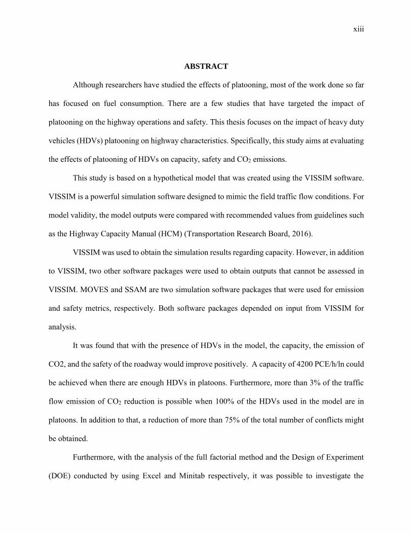
ABSTRACT

Although researchers have studied the effects of platooning, most of the work done so far

has focused on fuel consumption. There are a few studies that have targeted the impact of

platooning on the highway operations and safety. This thesis focuses on the impact of heavy duty

vehicles (HDVs) platooning on highway characteristics. Specifically, this study aims at evaluating

the effects of platooning of HDVs on capacity, safety and CO2 emissions.

This study is based on a hypothetical model that was created using the VISSIM software.

VISSIM is a powerful simulation software designed to mimic the field traffic flow conditions. For

model validity, the model outputs were compared with recommended values from guidelines such

as the Highway Capacity Manual (HCM) (Transportation Research Board, 2016).

VISSIM was used to obtain the simulation results regarding capacity. However, in addition

to VISSIM, two other software packages were used to obtain outputs that cannot be assessed in

VISSIM. MOVES and SSAM are two simulation software packages that were used for emission

and safety metrics, respectively. Both software packages depended on input from VISSIM for

analysis.

It was found that with the presence of HDVs in the model, the capacity, the emission of

CO2, and the safety of the roadway would improve positively. A capacity of 4200 PCE/h/ln could

be achieved when there are enough HDVs in platoons. Furthermore, more than 3% of the traffic

flow emission of CO2 reduction is possible when 100% of the HDVs used in the model are in

platoons. In addition to that, a reduction of more than 75% of the total number of conflicts might

be obtained.

Furthermore, with the analysis of the full factorial method and the Design of Experiment

(DOE) conducted by using Excel and Minitab respectively, it was possible to investigate the

xiv

impact of the platoons’ factors on the highway parameters. Most of these factors affect the

parameters significantly. However, the change in the desired speed was found to insignificantly

affect the highway parameters, due to the high penetration rate.

Keywords: VISSIM, MOVES, SSAM, COM-interface, HDVs, Platooning, Number of

Conflicts.

1

CHAPTER 1: INTRODUCTION

I. Background

Heavy-duty vehicles (HDVs) make transferring and shipping goods possible. They are

essential to the world economy, as they play a key role in transporting freight using surface

transportation. However, HDVs have adverse effects on highways, such as congestions, traffic

accidents, emissions pollution, etc. In spite of continuous endeavors from public authorities to

enhance the roadway infrastructure, the burden on infrastructure, energy usage, and the

environment is on the rise. This is due to the in the demand for road freight transport (Van Arem,

Van Driel, & Visser, 2006)

According to the Environmental Protection Agency (EPA), more than 28% of total U.S.

greenhouse gas emissions come from the transportation sector (EPA, 2018). Reducing pollutant

emissions to reach the respective national ambient air quality standard by 2020 is one of the main

objectives of EPA. The efficiency and improvement of freight transport trigger the attention of

public authorities, transport planners, researchers, and automotive manufacturers because the

freight transport by HDVs is one of the main policy areas for enhancement of overall energy

efficiency.

A “cooperative system” is one of the benefits of innovations of the Information and

Communication Technology (ICT) and applications for Intelligent Transportation Systems (ITS).

To enhance the performance of the traffic system, this cooperative system uses vehicle-to-vehicle

(V2V) and vehicle-to-infrastructure (V2I) communication (Farah et al., 2012). Due to its positive

effect on traffic safety, many studies have been committed to investigate the improvement and

2

implementation of a cooperative system. There are other expected benefits from the cooperative

system, such as the improving traffic flow and alleviating some environmental effects.

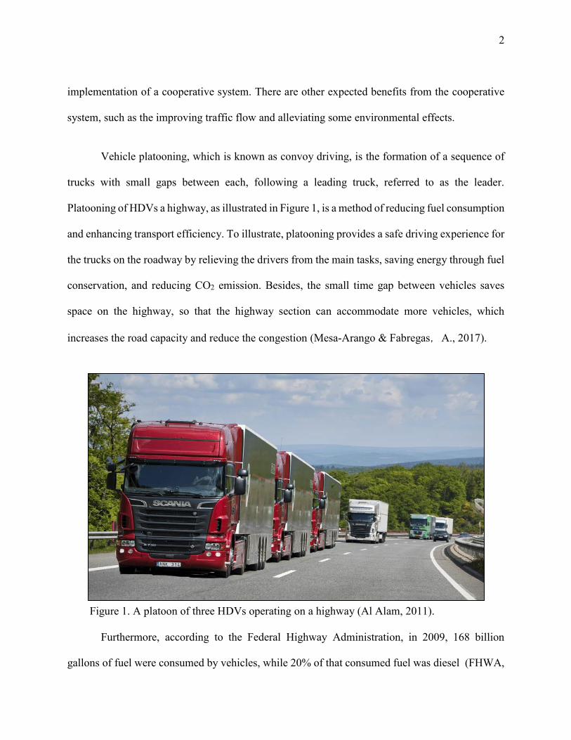
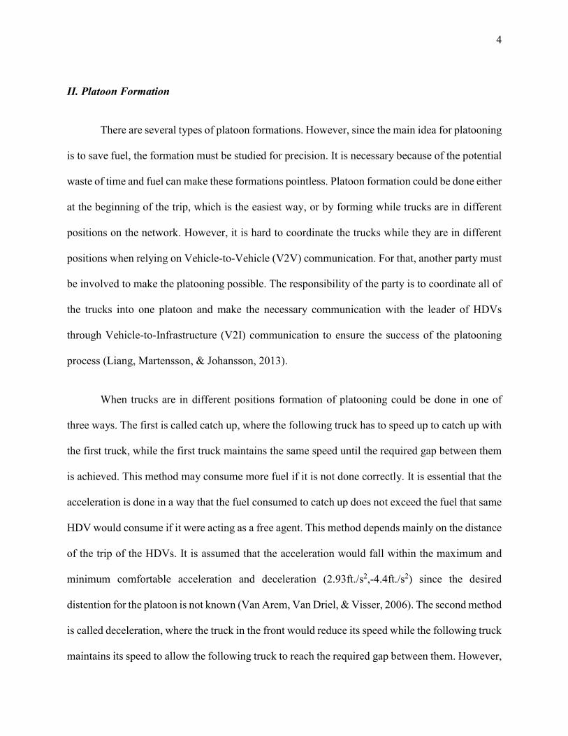
Vehicle platooning, which is known as convoy driving, is the formation of a sequence of

trucks with small gaps between each, following a leading truck, referred to as the leader.

Platooning of HDVs a highway, as illustrated in Figure 1, is a method of reducing fuel consumption

and enhancing transport efficiency. To illustrate, platooning provides a safe driving experience for

the trucks on the roadway by relieving the drivers from the main tasks, saving energy through fuel

conservation, and reducing CO2 emission. Besides, the small time gap between vehicles saves

space on the highway, so that the highway section can accommodate more vehicles, which

increases the road capacity and reduce the congestion (Mesa-Arango & Fabregas，A., 2017).

Figure 1. A platoon of three HDVs operating on a highway (Al Alam, 2011).

Furthermore, according to the Federal Highway Administration, in 2009, 168 billion

gallons of fuel were consumed by vehicles, while 20% of that consumed fuel was diesel (FHWA,

3

2019). By using HDVs platooning, fuel saving may reach up to 20% due to small time gap that

causes significant air-drag reduction, and therefore, reduces fuel consumption (Browand,

McArthur, & Radovich, 2004). Giving that the demand for freight transportation has been growing

every year, HDV platooning has already been considered as an effective way of reducing

environmental impacts. It is expected to be implemented in several states in the near future

(Lockwood, 2016). Therefore, an extensive study of the effect of the HDV platooning on the

highway`s parameters should be carefully analyzed.

Due to the complexity of platooning and the fact that it is a new innovation, many states

are cautious about allowing HDV platooning to be driven on its roads (Autonomous Vehicles |

Self-Driving Vehicles, 2019). In 2012, only six states passed the legislation for autonomous

vehicles to be used within their interstate highways. The State of Florida, for example, did not

consider permitting autonomous vehicles until 2016 with some limitations and requirements. In

item 316.0895 of the Florida legislation, the minimum safe distance between trucks is 300 feet.

However, item 316.85 stated that whoever has a valid driver license can operate an autonomous

vehicle in autonomous mode on the state roads, if the vehicle is equipped with autonomous

technology, such as adaptive cruise control (ACC). Furthermore, item 316.0896 illustrates some

limitations on using platooning on Florida highways, such as submitting insurance to the

Department of Highway Safety and Motor Vehicles with an amount of five million dollars (Florida

legislature, 2019).

4

II. Platoon Formation

There are several types of platoon formations. However, since the main idea for platooning

is to save fuel, the formation must be studied for precision. It is necessary because of the potential

waste of time and fuel can make these formations pointless. Platoon formation could be done either

at the beginning of the trip, which is the easiest way, or by forming while trucks are in different

positions on the network. However, it is hard to coordinate the trucks while they are in different

positions when relying on Vehicle-to-Vehicle (V2V) communication. For that, another party must

be involved to make the platooning possible. The responsibility of the party is to coordinate all of

the trucks into one platoon and make the necessary communication with the leader of HDVs

through Vehicle-to-Infrastructure (V2I) communication to ensure the success of the platooning

process (Liang, Martensson, & Johansson, 2013).

When trucks are in different positions formation of platooning could be done in one of

three ways. The first is called catch up, where the following truck has to speed up to catch up with

the first truck, while the first truck maintains the same speed until the required gap between them

is achieved. This method may consume more fuel if it is not done correctly. It is essential that the

acceleration is done in a way that the fuel consumed to catch up does not exceed the fuel that same

HDV would consume if it were acting as a free agent. This method depends mainly on the distance

of the trip of the HDVs. It is assumed that the acceleration would fall within the maximum and

minimum comfortable acceleration and deceleration (2.93ft./s2,-4.4ft./s2) since the desired

distention for the platoon is not known (Van Arem, Van Driel, & Visser, 2006). The second method

is called deceleration, where the truck in the front would reduce its speed while the following truck

maintains its speed to allow the following truck to reach the required gap between them. However,

5

that could be considered a waste of time but would guarantee less fuel consumption for the whole

platoon. The third and most suitable method is a combination of the first two methods. It is done

by reducing the speed of the leader truck by a reasonable speed and speeding up the following

truck to the desired speed to reach the desired gap distance with the help of the coordinator. The

first two ways use (ACC) while the third one uses Cooperative Adaptive Cruise Control (CACC)

(Van Arem, Van Driel, & Visser, 2006).

III. Research Objectives

Platooning studies have been conducted for the past 50 years. However, the majority of

those studies have been devoted to the implementations and the development of the platooning

system. Very few studies have been conducted to investigate the impact of platooning on traffic

flow. Those studies focused mainly on cars platooning without concentration on environmental

impacts. HDV platooning impact on traffic flow (such as capacity, safety, and greenhouse

emissions), still have been insufficiently studied (Mesa-Arango & Fabregas, 2017). Insufficient

information has been found regarding the impacts of HDV platoon operations on traffic flow on

highways. Apart from fuel saving, there are many topics regarding HDV platooning that need to

be investigated.

For the sake of understanding the HDV platooning impact on highway parameters, this

thesis is based on designing and simulation of HDV platooning, using primarily utilizing VISSIM

software. The study focusses on the impact of HDV platooning on highways regarding the

capacity, safety, and greenhouse gas emissions. Additionally, the study will investigate the

significance of other HDV platooning variables on highway parameters: percentage of trucks of

6

the traffic flow, percentage of platoons, the time gap, the speed of the platoons, and the number of

trucks within a single platoon.

IV. Thesis Limitations and Framework

This thesis is based on simulation and modeling. The study uses a hypothetical model. For

simplicity, the model does not include ramps. In order to neglect the effect of the ramps on the

highway movement, such as weaving. Besides, there were assumed only two vehicle types

available in the traffic mix of the highway: passenger cars and trucks. The characteristics of heavy-

HDV (such as refrigerator trucks), were chosen for the simulation and analysis. Heavy-HDVs have

a weight of more than 33,000 lb. (class 8). This thesis did not investigate the formation of the

platoon effect on the highway movement. During all the simulation runs, it was assumed the

platoon formation was created before entering the hypothetical model. Furthermore, in the study

of the effect of HDV platooning on emission, MOVES simulation software was used. For accurate

results, the effect of air drag reduction should be taken into consideration. However, MOVES does

not have an input for air drag calculations. Therefore, the reduction of fuel consumption of HDV

platooning was used, based on ITS energy project (Tsugawa, 2013), to estimate the reduction of

air drag. Furthermore, it is preferred that trucks drive in the outer lane, it was assumed that the

platoons would be driven in the right lane and would not be allowed to use the left lane or do a

lane change during the simulation.

This thesis aims to study the HDV platooning effects on traffic flow parameters on the

highway. The outline of this thesis will discuss the implementation of the simulation and the steps

of collecting the results in a few chapters as follows:

7

Chapter 2: Background

This chapter defines HDV platooning parameters, mentions some of the benefits of truck

platooning, and illustrates the related work about HDV platooning, such as studies related to fuel

saving and the formation of HDV platooning.

Chapter 3: Methodology

This chapter explains the simulation software packages that were used. It includes defining

properties and operations of HDV platoons, modeling of ACC/CACC systems considering the

acceleration capability, and how they have been used within VISSIM, SSAM and MOVES

software. Furthermore, it describes the methodology that was used to collect and analyze the

outcomes.

Chapter 4: The Impact of HDV platooning on Traffic Flow Parameters

This chapter presents the outcomes that were collected from the simulations and discusses

the impact of HDVs on capacity, safety and the greenhouse emissions based on the outcomes. It

compares the results of different scenarios of different percentages of HDV platoons’ impact on

highway traffic flow parameters.

Also, five factors of HDV platoons were statically analyzed to investigate which of these

factors have a significant impact on the rate of change on traffic flow parameters. The analysis of

the “factorial method” was implemented to discuss the impact. The five factors chosen are as

follow: the percentage HDVs trucks from all the traffic flow within the simulation, percentage of

HDV platoon from all trucks, the time gap between HDVs within the platoon, and the desired

speed of traffic flows , and the number of HDVs within a platoon.

8

Chapter 5: Overall Conclusions and Future Work

This chapter summarize the thesis work, and the thesis steps with some concluding

remarks, and gives some recommendations for future work.

9

CHAPTER 2: BACKGROUND

I. Heavy Duty Vehicle Development

Truck platooning involves the formation of a sequence of trucks with a small time gap

between each other, following a leading truck, referred to as the leader. The following trucks

instantly mimic the movement of the leader. The main idea of platooning is to provide a safe

driving experience for the trucks on the roadway, save energy through fuel conservation, and

reduce CO2 emission. Additional benefits are the increase in roadway capacity and congestion

reduction (Mesa-Arango & Fabregas, 2017).

Since the 1970s, ITS research has been attracted to vehicle platooning topics, with some

general interest about severe traffic around major urban centers. The concept of fully automated

vehicles traveling in platoons using electronic coupling began in the 1970s (Garrard, 1979). One

of the pioneering studies in platooning was conducted by the California Partners for Advanced

transportation TecHnology (PATH) initiative which started in 1986. At the beginning of the

project, the interest was only on cars platooning. However, the HDV became a part of the plan

later, with the main objective of enhancing traffic conditions in California. The focus for

platooning research has since shifted from cars to HDVs, specifically aiming at reducing the

aerodynamic resistance (Shladover et al., 1991). The experiment was done in San Diego in on an

empty freeway with two lanes, and with platooning of three to eight automated trucks with the

speed of about 96 km/h (60 mi/h) with each truck weighing 25 ton. The platooning was driving

with a gap distance of 6.3 m to see the effect of the aerodynamic on fuel saving. California PATH

gave indications that a traffic volume of 1800 to 2000 veh/h/ln could be doubled or tripled if there

were 100% of HDV platooning only in the freeway (Van Arem, Van Driel, & Visser, 2006).

10

Another valuable project that started in 2013 was known as the COoperative dynamic forMation

of Platoons for sAfe and energy-optImized goods transportatioN (COMPANION). The European

Commission sponsored the COMPANION initiative. The main objective was to investigate the

risk of changing the regulation to allow shorter time gaps within HDV platoons. Taking into

consideration traffic information and weather conditions, the project was aimed at establishing a

dynamic coordination system. The idea of forming a platoon developed organically within the

project. HDVs within Such a platoon might not necessarily to have the same origin or destination

for HDVs within the platoon. Furthermore, the projects aimed to study the capability of the

Human-Machine interface (HMI).

II. Related Studies

There are many studies conducted on platooning, either car platooning or HDV platooning.

In this section, three studies are explored regarding the three parameters of this analyzed in this

thesis. Starting with capacity, Zhao and Sun (2013) conducted a study that focused on vehicle

platooning and car-following behaviors on capacity. In addition, Van Nunen, Esposto, Saberi, and

Paardekooper (2017) discussed the safety of HDVs from the perspectives of roadway breaks and

slopes. In addition, the emission of CO2 was studied on real HDV platooning in Energy ITS project

in 2009 (Tsugawa)

III. Effect of Car Platooning on Capacity

While car platooning has become an interest of the majority of the automobile industry,

the absolute result of platooning impact on traffic flow capacity remains unclear. In Simulation

Framework for Vehicle Platooning and car-following behaviors, Zhao (2013) researched and

discussed the effect of passenger cars on roadway capacity. The goal of Zhao’s study was to model

a simulation framework of CACC platoon by using the application programming interface in

11

microscopic-traffic simulation. Six vehicles equipped with CACC in a platoon were simulated to

study the interaction of the platoon in traffic stream and to microscopically study the shockwave

reaction of the interaction. It was assumed that vehicles equipped with CACC do not change lanes

during the simulations. The results indicated that the platoon increased the lane capacity

significantly at higher penetration rates of CACC vehicles. However, platoon size had little impact

on traffic capacity.

like the above study, this thesis uses a simulation model for the outcomes. However, this

thesis investigates the effect of HDVs instead of passenger cars. Likewise, just as the study did not

car include lane changing, this thesis includes the assumption of no HDV platoon lane change.

IV. Implementation of HDVs with Safety

The safety of roadways is one of the main factors that concerns traffic engineers. There is

one study that investigated HDV platooning safety during the formation of the platooning (Liang,

Mårtensson, & Johansson, 2016). The study was conducted to illustrate the effects of slope and

break on the safety of the platoon. It was proposed that two-layer control architecture for HDV

platooning aimed to safely and fuel-efficiently coordinate the vehicles in the platoon. The proposed

layers were responsible for the real-time control of the vehicles and the inclusion of preview

information on road topography. The study showed that the proposed layer would give safer

conditions to control the platoon and would save about 12% of gasoline compared to using a

standard platooning controller.

12

Unlike the above study, this thesis investigates the safety of the highway traffic flow with

the implementation of HDV platooning. Furthermore, the thesis aims to include the factors that

have the most significant impact on highway safety.

V. CO2 Emission within Energy ITS

Another significant HDV platooning study was “Energy ITS.” Energy ITS started in Japan

in 2008 after CO2, which is one of the main elements that causes global warming, had reached

high levels of emission in Japan’s environment. In 2011, it was found that around 28% of the CO2

emissions nationwide comes from the transportation sector (Tsugawa, 2013). More than 6% came

from trucks (Tsugawa, Jeschke, & Shladover, 2016). The main objective of “Energy ITS” was to

save energy by reducing energy consumption and preventing global warming with automated

driving. In 2008, ”Energy ITS” conducted an experiment on three trucks driving in a platoon on a

roadway with their speed set around 80 km/h (50 mi/h); gap distance varied between 4.7m and

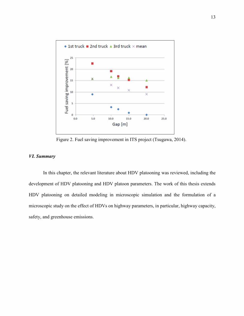
20m (15.42 ft. and 65.62 ft.). Figure 2 represents the fuel saved after running the experiment on

unloaded trucks with a constant speed of around 80 km/h (50 mi/h). The figure shows that the

mean of the fuel saving was around 16% when the gap distance was 4.7m (15.42 ft.) and 13%

when the distance was around 10m (32.82 ft.). CO2 emission reduction was measured, and the

experiment showed that up to 4.8% of the CO2 emissions were reduced when the gap was 4m

(13.12 ft.) and 2.1% when the gap was 10m (32.81 ft.) (Sadayuki, 2013).

13

Figure 2. Fuel saving improvement in ITS project (Tsugawa, 2014).

VI. Summary

In this chapter, the relevant literature about HDV platooning was reviewed, including the

development of HDV platooning and HDV platoon parameters. The work of this thesis extends

HDV platooning on detailed modeling in microscopic simulation and the formulation of a

microscopic study on the effect of HDVs on highway parameters, in particular, highway capacity,

safety, and greenhouse emissions.

14

CHAPTER 3: MODELING

This chapter illustrates the methodology that was used in this study. It is divided into three

main sections. The first section presents the principles of HDV platooning, while the second

section discusses the simulation process. The third section shows the calibration and validation of

the simulation model. The three software packages used in this study are VISSIM, MOVES, and

SSAM. The last two software packages depend on the outcomes of the first one. They were used

to study the impact of HDV platooning on capacity, emission rate, and safety.

I. Heavy Duty Vehicles Platoon Operations

This subsection describes the operation of HDV platooning and the software packages

used. Additionally, it highlights the method of connection and communication between HDVs in

platoons.

A. The Operations of HDVs

HDV platooning consisted of a group of HDVs driving close to each other and being

controlled as one unit, i.e., all vehicles in the platoon mimic the lead vehicle. The HDV platoon

was modeled as a platoon class/structure, which represents a group of HDVs with the platooning

capability. The traffic model implemented has the ability to mirror the driving behaviors

(operations) of an HDV platoon. It includes the acceleration, deceleration, maintaining the time

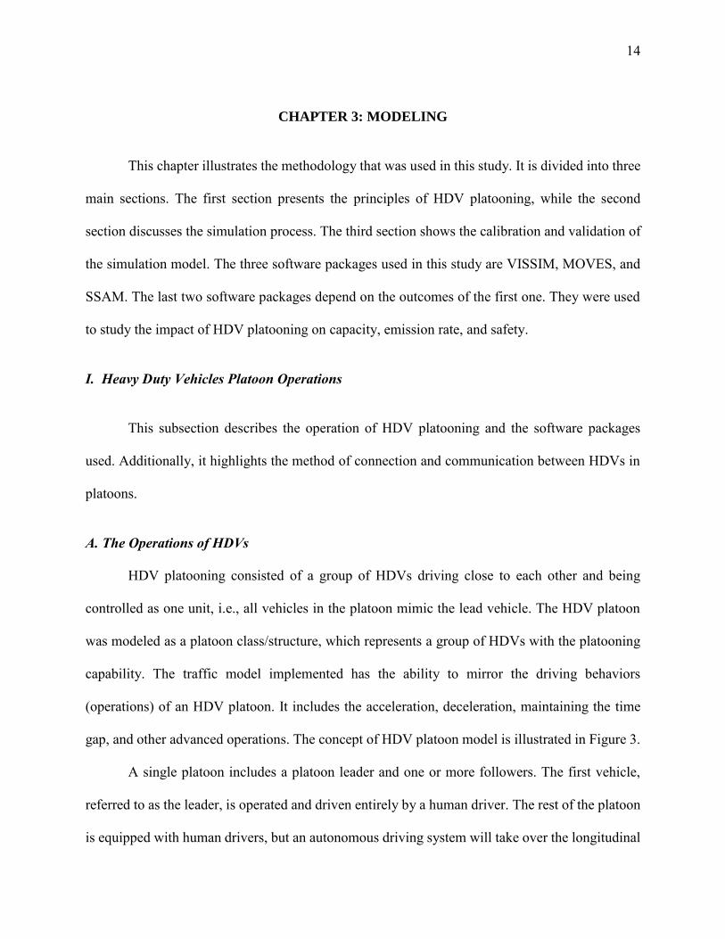
gap, and other advanced operations. The concept of HDV platoon model is illustrated in Figure 3.

A single platoon includes a platoon leader and one or more followers. The first vehicle,

referred to as the leader, is operated and driven entirely by a human driver. The rest of the platoon

is equipped with human drivers, but an autonomous driving system will take over the longitudinal

15

driving tasks. The drivers of the followers can take control when they want to join or leave the

platoon.

As shown in Figure 3, the HDV platoon consists of three main properties: platoon leader

ID, platoon speed, and the list of HDV platoon members. Since the speed of the trucks within the

same platoon may be different, the speed of the platoon is related to the leader’s speed. Each

vehicle in the HDV platoon has its information stored in the HDV platoon members list.

Figure 3. The HDV platoon model with its properties and operations.

In the study, all HDV platoons are initiated and operated by the platoon leader. It is the

primary job of the leader to accelerate, decelerate, and maintain the platoon in the required lanes.

For example, when a platoon reaches congestion, the leader makes the decision to change the lane

or keep using the same lane for the whole platoon. For safety purposes, it was assumed that

platoons would drive only on the outer lane to allow free agent vehicles (especially passenger cars)

to drive in the inside lane -- the fast lane.

16

B. Platooning System

In the late 1970s, the concept of fully automated vehicles traveling in platoon using

electronic coupling emerged (Caudill & Garrard, 2010). With the development of HDV

platooning, the concept of Adaptive Cruise Control (ACC) has become an essential part of the

platoon. Another advance system of ACC was joined and named Cooperative Adaptive Cruise

Control (CACC). This section discusses the implementation of these systems and how they can

affect the HDV platoons.

1. ACC System

When an HDV joins a platoon, an autonomous driving system, ACC, will take over the

longitudinal driving tasks. ACC is a radar-based system, which is designed to enhance the

driving by relieving the driver from the main tasks, such as adjusting the time gap, and the

desired speed (Van A., et al., 2006). The system was designated to slow down when a

follower reaches a certain set distance and increases the speed when the proceeding vehicle

disappears (e.g., changing lane).

Van Arem, Van Driel, and Visser have proposed an equation (see Equation 1) for

the acceleration demand (2006), which is based on relative speed and deviation of current

distance from the desired vehicle gap.

𝑎𝑎𝑐𝑐 = 𝑘𝜈 · (𝜈𝑝 − 𝜈) + 𝑘𝑑 · (𝑟 − 𝑟𝑟𝑒𝑓) (1)

The values of 𝑘𝜈 and 𝑘𝑑 are control parameters that must be empirically

configured, while the values of 𝜈𝑝 and 𝜈 are the velocity of the proceeding vehicle and

controlled vehicle respectively. The distance between the two vehicles is referred to as 𝑟.

and 𝑟𝑟𝑒𝑓 is the the least of rmin (2) and rsystem (0.5 × desired speed)

.

17

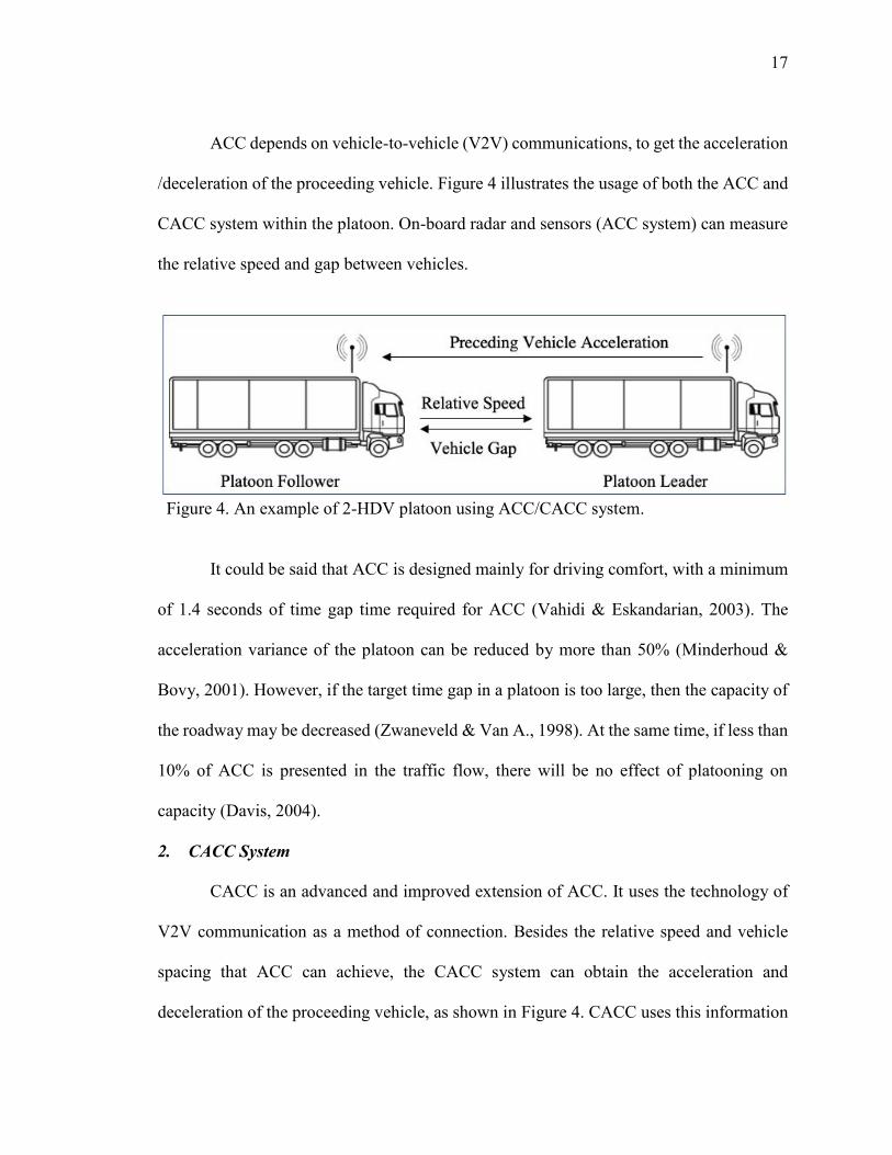
ACC depends on vehicle-to-vehicle (V2V) communications, to get the acceleration

/deceleration of the proceeding vehicle. Figure 4 illustrates the usage of both the ACC and

CACC system within the platoon. On-board radar and sensors (ACC system) can measure

the relative speed and gap between vehicles.

Figure 4. An example of 2-HDV platoon using ACC/CACC system.

It could be said that ACC is designed mainly for driving comfort, with a minimum

of 1.4 seconds of time gap time required for ACC (Vahidi & Eskandarian, 2003). The

acceleration variance of the platoon can be reduced by more than 50% (Minderhoud &

Bovy, 2001). However, if the target time gap in a platoon is too large, then the capacity of

the roadway may be decreased (Zwaneveld & Van A., 1998). At the same time, if less than

10% of ACC is presented in the traffic flow, there will be no effect of platooning on

capacity (Davis, 2004).

2. CACC System

CACC is an advanced and improved extension of ACC. It uses the technology of

V2V communication as a method of connection. Besides the relative speed and vehicle

spacing that ACC can achieve, the CACC system can obtain the acceleration and

deceleration of the proceeding vehicle, as shown in Figure 4. CACC uses this information

18

to achieve the required small time gap while maintaining stable platooning. Ploeg (2011)

investigated and evaluated the CACC on a six-vehicle platoon. This study showed that 0.5

seconds of time gap could be achieved with V2V communication using the CACC system.

This small time gap can be achieved by maintaining a stable platoon (Ploeg et al., 2011).

Equations 2, 3 and 4 are used in the simulation model for this thesis. These

equations were used by (Van Arem et al., 2006) to achieve the minimum stabled time gap

of 0.5 seconds in platoons.

𝑎𝑟𝑒𝑓 = 𝑚𝑖𝑛 (𝑎𝑟𝑒𝑓_𝜈, 𝑎𝑟𝑒𝑓_𝑑) (2)

𝑎𝑟𝑒𝑓𝜈 = 𝑘 · (𝜈𝑖𝑛𝑡 − 𝜈) (3)

𝑎𝑟𝑒𝑓_𝑑 = 𝑘𝑎 · 𝑎𝑝 + 𝑘𝜈 · (𝜈𝑝 − 𝜈) + 𝑘𝑑 · (𝑟 − 𝑟𝑟𝑒𝑓) (4)

Equation 2 is used for the acceleration of the following HDVs to catch up with the

HDVs upstream and join or form a platoon, keeping the time gap of 0.5 seconds. It takes

the minimum between Equation 2 and 3. In those equations, k = 1, νint and ν are the

intended velocity and the current velocity of the following HDVs respectively. Ka = 1,

while kν and kd values are 0.58 and 0.1 respectively. Where νp is the velocity of the

predecessor HDVs and r is the net distance between the two HDVs, rref is the maximum

value between rmin and rsystem, where rmin =2 and rsystem = 0.5 ·ν.

In this thesis, the CACC System is used as the default connection between the

vehicles in the platoon. The reason for this assumption is that ACC connection showen in

previous studies, that it does not have a significant effect on the traffic flow regardless of

the set time gap between the vehicles (Van A. et al., 2006).

19

III. Simulation Software

This thesis is conducted based on three main simulation software: VISSIM, MOVES, and

SSAM. This section is divided into three subsections. Each section explains and clarifies how the

software works and how they have been used for the study. First, VISSIM was used to build a

hypothetical model that has defined characteristics to measure the effect of HDV platooning on

capacity. Secondly, MOVES is an EPA simulation software designed to measure the effect of

traffic movement on the environment. Finally, SSAM was designed by FHWA to investigate the

safety of traffic movement. The validity of these software packages was investigated by different

studies (Huang, Liu, Yu, & Wang, 2013).

A. VISSIM

VISSIM is a powerful traffic simulation tool that is used in the analysis of the transport

system. The software has been used in different ITS-based vehicle studies. Precisely, it

provides a high profile of microscopic details of the simulated traffic flow. VISSIM mirrors

the traffic pattern of medium traffic flow. Since VISSIM has the ability to mimic the

psychophysical car-following model and lane-changing model to determine longitudinal

and lateral driving behaviors of passenger vehicles, VISSIM is used as the backbone of this

thesis. It is used to analyze the mixed traffic movement to obtain capacity data for different

scenarios. Besides, VISSIM model is used to simulate the traffic movement to study the

effect of HDVs on safety and emission as explained below. VISSIM COM server interface

is used to perform the HDV platoon behavior, especially when VISSIM does not permit

such a small time gap. The COM interface enables users to access and reshape traffic

20

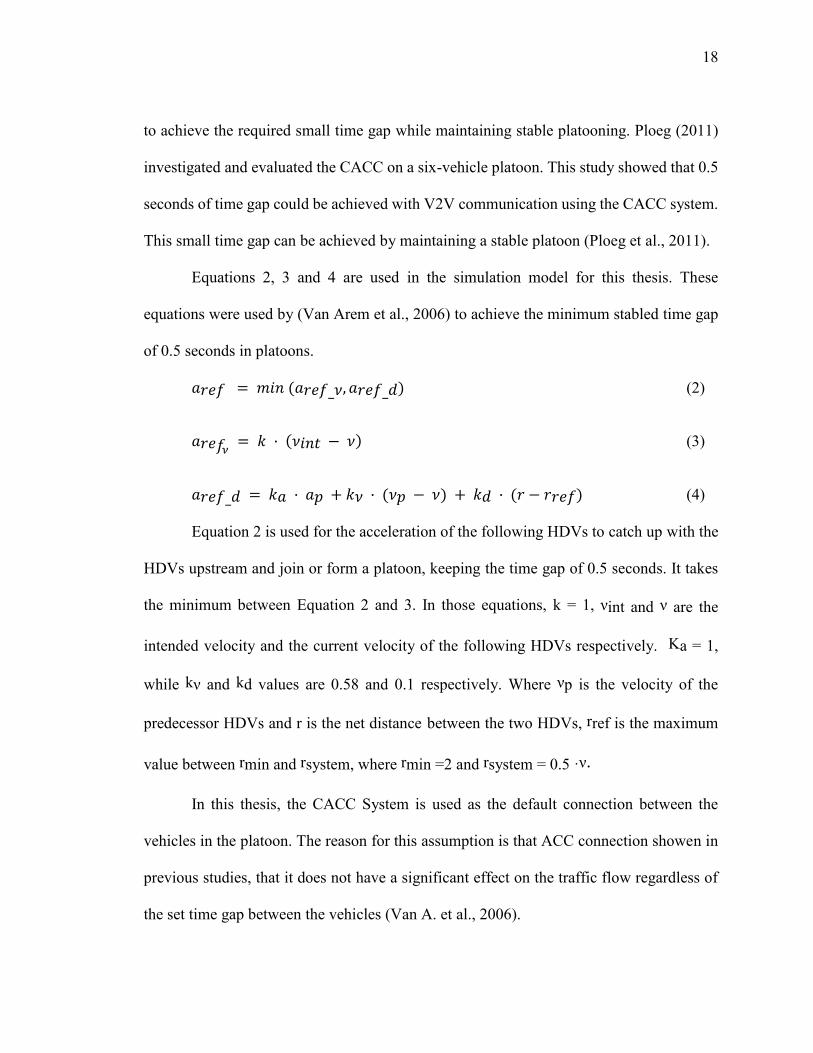
driving behavior. The interaction between COM interface and VISSIM can be seen in

Figure 5.

Figure 5. The interaction between VISSIM and COM interface.

The validity of the VISSIM model was tested to insure the legitimacy of the

simulation outcomes. The method of validity is illustrated, with details, in the HDV Platoon

Model section (page 28).

B. MOVES

The MOtor Vehicle Emission Simulator (MOVES) is a state-of-the-art modeling

framework. It was designed to allow easier incorporation of large amounts of in-use data

from a variety of sources (Hall & Noel, 2014). MOVES was designed and tested by the

21

United State Environmental Protection Agency (EPA), and its primary purpose is the

development of a new emission factor and inventory model for free source emissions.

According to the EPA website, MOVES was defined as the “state-of-the-science emission

modeling system that estimates emissions for mobile sources at the national, county, and

project level for criteria air pollutants, greenhouse gases, and air toxics” (EPA, 2017). Air

pollution modelers within the U.S. at local levels can use the model. To run MOVES, users

must provide or create a run specification (RunSpec) that describes the nature of the

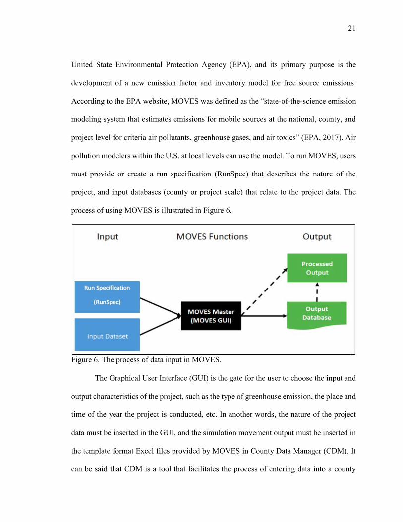
project, and input databases (county or project scale) that relate to the project data. The

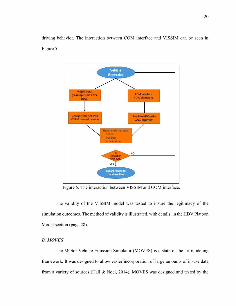
process of using MOVES is illustrated in Figure 6.

Figure 6. The process of data input in MOVES.

The Graphical User Interface (GUI) is the gate for the user to choose the input and

output characteristics of the project, such as the type of greenhouse emission, the place and

time of the year the project is conducted, etc. In another words, the nature of the project

data must be inserted in the GUI, and the simulation movement output must be inserted in

the template format Excel files provided by MOVES in County Data Manager (CDM). It

can be said that CDM is a tool that facilitates the process of entering data into a county

22

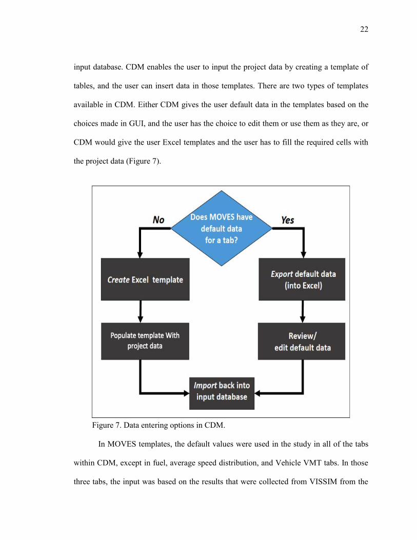
input database. CDM enables the user to input the project data by creating a template of

tables, and the user can insert data in those templates. There are two types of templates

available in CDM. Either CDM gives the user default data in the templates based on the

choices made in GUI, and the user has the choice to edit them or use them as they are, or

CDM would give the user Excel templates and the user has to fill the required cells with

the project data (Figure 7).

Figure 7. Data entering options in CDM.

In MOVES templates, the default values were used in the study in all of the tabs

within CDM, except in fuel, average speed distribution, and Vehicle VMT tabs. In those

three tabs, the input was based on the results that were collected from VISSIM from the

23

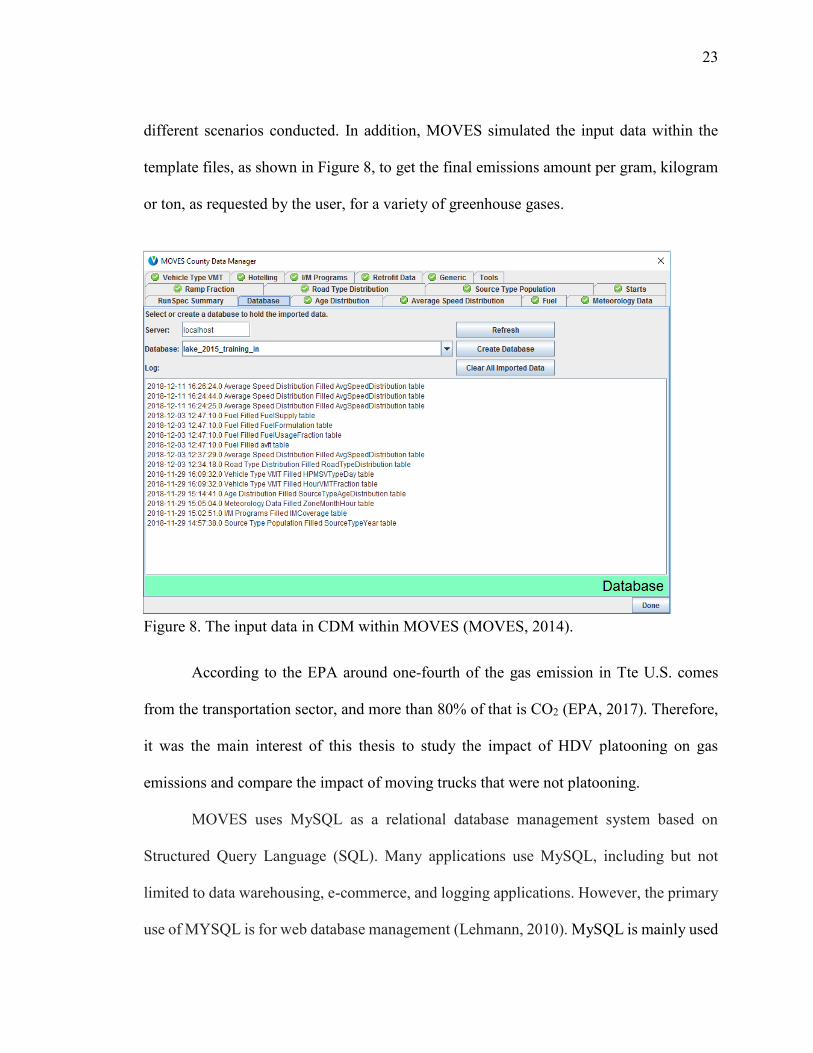
different scenarios conducted. In addition, MOVES simulated the input data within the

template files, as shown in Figure 8, to get the final emissions amount per gram, kilogram

or ton, as requested by the user, for a variety of greenhouse gases.

Figure 8. The input data in CDM within MOVES (MOVES, 2014).

According to the EPA around one-fourth of the gas emission in Tte U.S. comes

from the transportation sector, and more than 80% of that is CO2 (EPA, 2017). Therefore,

it was the main interest of this thesis to study the impact of HDV platooning on gas

emissions and compare the impact of moving trucks that were not platooning.

MOVES uses MySQL as a relational database management system based on

Structured Query Language (SQL). Many applications use MySQL, including but not

limited to data warehousing, e-commerce, and logging applications. However, the primary

use of MYSQL is for web database management (Lehmann, 2010). MySQL is mainly used

24

to communicate with a database, and it is the standard language for relational database

management systems. MYSQL statements are used to perform tasks such as updating data

in a database or retrieving data from a database. It was used in this study to analyze and

group the results that were found from MOVES and to compare the final CO2 emissions in

different scenarios.

C- SSAM

For the effect of the HDV platooning on the overall traffic safety, the same model

of VISSIM was used with the addition of another simulation software called Surrogate

Safety Assessment Model (SSAM). Crashes are rare events, which means it takes a long

time to collect enough data to make reliable inference on the safety condition. Besides,

from the limitations in the data collection, assessment of traffic safety from traffic accidents

cannot be categorized as active safety management. The use of traffic safety indicators,

known merely as Surrogate Safety Measures (SSM), can increase the probability of

evaluating traffic safety changes more efficiently and in a shorter time (Peng, Abdel-Aty,

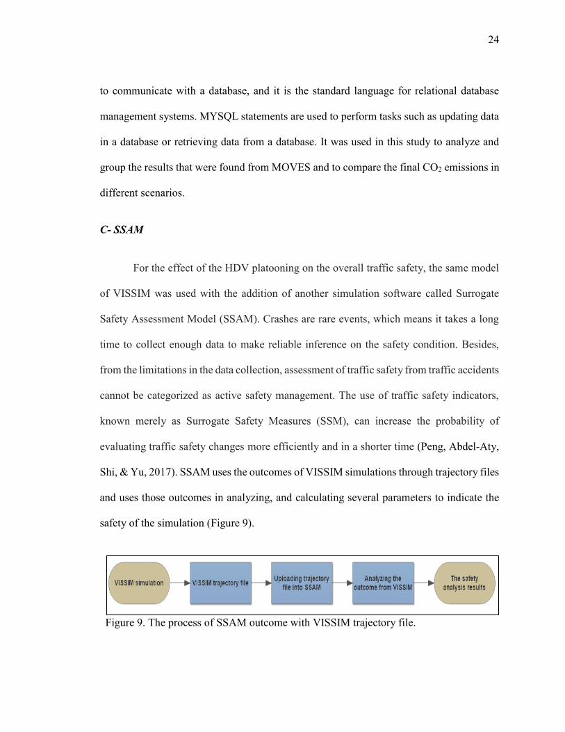
Shi, & Yu, 2017). SSAM uses the outcomes of VISSIM simulations through trajectory files

and uses those outcomes in analyzing, and calculating several parameters to indicate the

safety of the simulation (Figure 9).

Figure 9. The process of SSAM outcome with VISSIM trajectory file.

25

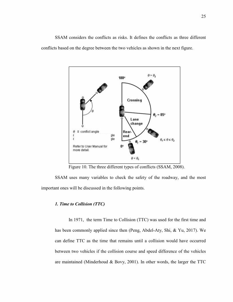
SSAM considers the conflicts as risks. It defines the conflicts as three different

conflicts based on the degree between the two vehicles as shown in the next figure.

Figure 10. The three different types of conflicts (SSAM, 2008).

SSAM uses many variables to check the safety of the roadway, and the most

important ones will be discussed in the following points.

1. Time to Collision (TTC)

In 1971, the term Time to Collision (TTC) was used for the first time and

has been commonly applied since then (Peng, Abdel-Aty, Shi, & Yu, 2017). We

can define TTC as the time that remains until a collision would have occurred

between two vehicles if the collision course and speed difference of the vehicles

are maintained (Minderhoud & Bovy, 2001). In other words, the larger the TTC

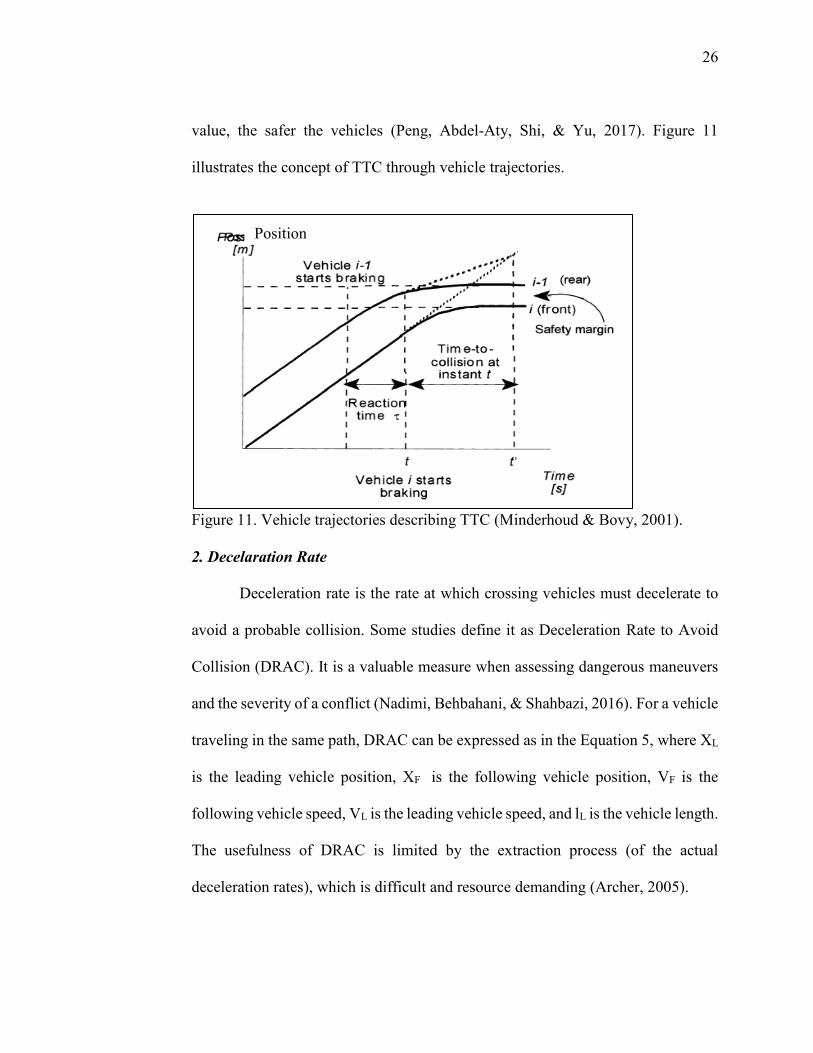
26

value, the safer the vehicles (Peng, Abdel-Aty, Shi, & Yu, 2017). Figure 11

illustrates the concept of TTC through vehicle trajectories.

Figure 11. Vehicle trajectories describing TTC (Minderhoud & Bovy, 2001).

2. Decelaration Rate

Deceleration rate is the rate at which crossing vehicles must decelerate to

avoid a probable collision. Some studies define it as Deceleration Rate to Avoid

Collision (DRAC). It is a valuable measure when assessing dangerous maneuvers

and the severity of a conflict (Nadimi, Behbahani, & Shahbazi, 2016). For a vehicle

traveling in the same path, DRAC can be expressed as in the Equation 5, where XL

is the leading vehicle position, XF is the following vehicle position, VF is the

following vehicle speed, VL is the leading vehicle speed, and lL is the vehicle length.

The usefulness of DRAC is limited by the extraction process (of the actual

deceleration rates), which is difficult and resource demanding (Archer, 2005).

Position

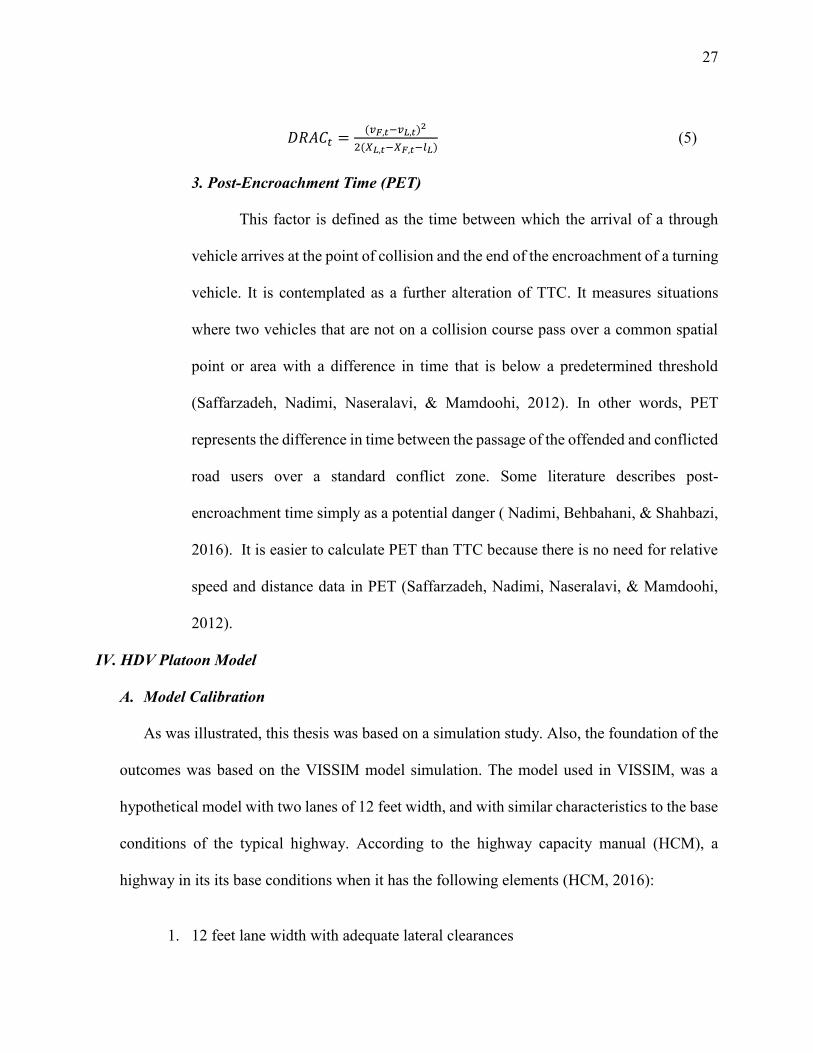
27

𝐷𝑅𝐴𝐶𝑡 =(𝑣𝐹,𝑡−𝑣𝐿,𝑡)2

2(𝑋𝐿,𝑡−𝑋𝐹,𝑡−𝑙𝐿) (5)

3. Post-Encroachment Time (PET)

This factor is defined as the time between which the arrival of a through

vehicle arrives at the point of collision and the end of the encroachment of a turning

vehicle. It is contemplated as a further alteration of TTC. It measures situations

where two vehicles that are not on a collision course pass over a common spatial

point or area with a difference in time that is below a predetermined threshold

(Saffarzadeh, Nadimi, Naseralavi, & Mamdoohi, 2012). In other words, PET

represents the difference in time between the passage of the offended and conflicted

road users over a standard conflict zone. Some literature describes post-

encroachment time simply as a potential danger ( Nadimi, Behbahani, & Shahbazi,

2016). It is easier to calculate PET than TTC because there is no need for relative

speed and distance data in PET (Saffarzadeh, Nadimi, Naseralavi, & Mamdoohi,

2012).

IV. HDV Platoon Model

A. Model Calibration

As was illustrated, this thesis was based on a simulation study. Also, the foundation of the

outcomes was based on the VISSIM model simulation. The model used in VISSIM, was a

hypothetical model with two lanes of 12 feet width, and with similar characteristics to the base

conditions of the typical highway. According to the highway capacity manual (HCM), a

highway in its its base conditions when it has the following elements (HCM, 2016):

1. 12 feet lane width with adequate lateral clearances

28

2. Drivers are in a regular composition and familiar with the roadway

3. No pavement deterioration

4. No work zone or accidents are present

5. Good weather conditions with excellent visibility to the drivers

6. No HDVs in the traffic stream

The model used in VISSIM has the characteristics of a base condition highway, except

with the presence of HDVs. To illustrate the model validity, a preliminary model was

designed with the whole highway in base condition (without the presence of HDVs). Based

on the exhibit 12-4 in HCM, the capacity of highway with the base condition was different

based on its Free Flow Speed (FFS) as in table 1:

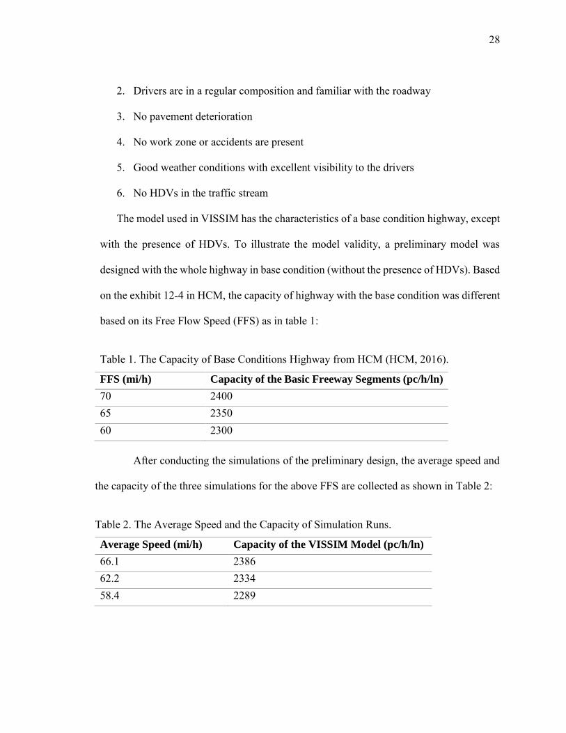
Table 1. The Capacity of Base Conditions Highway from HCM (HCM, 2016).

FFS (mi/h) Capacity of the Basic Freeway Segments (pc/h/ln)

70 2400 65 2350 60 2300

After conducting the simulations of the preliminary design, the average speed and

the capacity of the three simulations for the above FFS are collected as shown in Table 2:

Table 2. The Average Speed and the Capacity of Simulation Runs.

Average Speed (mi/h) Capacity of the VISSIM Model (pc/h/ln)

66.1 2386 62.2 2334 58.4 2289

29

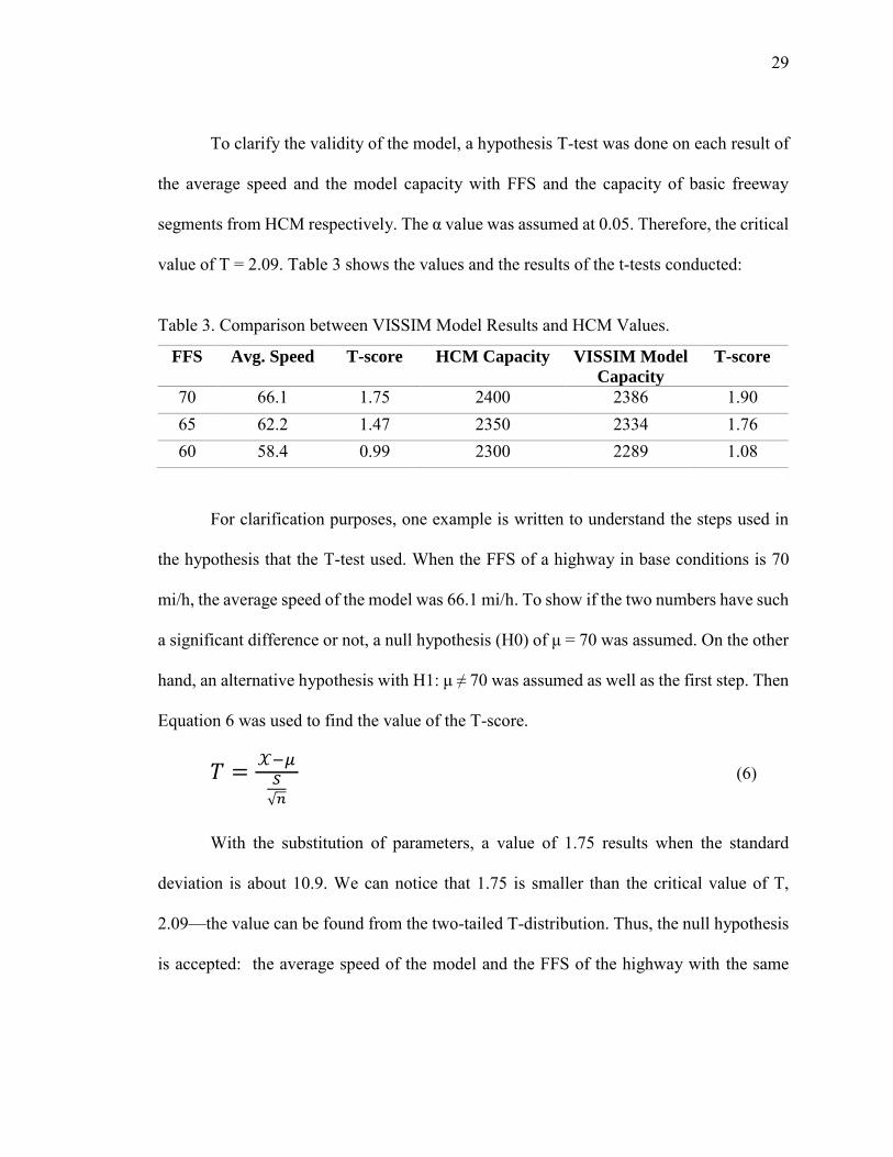
To clarify the validity of the model, a hypothesis T-test was done on each result of

the average speed and the model capacity with FFS and the capacity of basic freeway

segments from HCM respectively. The α value was assumed at 0.05. Therefore, the critical

value of T = 2.09. Table 3 shows the values and the results of the t-tests conducted:

Table 3. Comparison between VISSIM Model Results and HCM Values.

FFS Avg. Speed T-score HCM Capacity VISSIM Model

Capacity

T-score

70 66.1 1.75 2400 2386 1.90 65 62.2 1.47 2350 2334 1.76 60 58.4 0.99 2300 2289 1.08

For clarification purposes, one example is written to understand the steps used in

the hypothesis that the T-test used. When the FFS of a highway in base conditions is 70

mi/h, the average speed of the model was 66.1 mi/h. To show if the two numbers have such

a significant difference or not, a null hypothesis (H0) of μ = 70 was assumed. On the other

hand, an alternative hypothesis with H1: μ ≠ 70 was assumed as well as the first step. Then

Equation 6 was used to find the value of the T-score.

𝑇 =𝒳−𝜇

𝑆

√𝑛

(6)

With the substitution of parameters, a value of 1.75 results when the standard

deviation is about 10.9. We can notice that 1.75 is smaller than the critical value of T,

2.09—the value can be found from the two-tailed T-distribution. Thus, the null hypothesis

is accepted: the average speed of the model and the FFS of the highway with the same

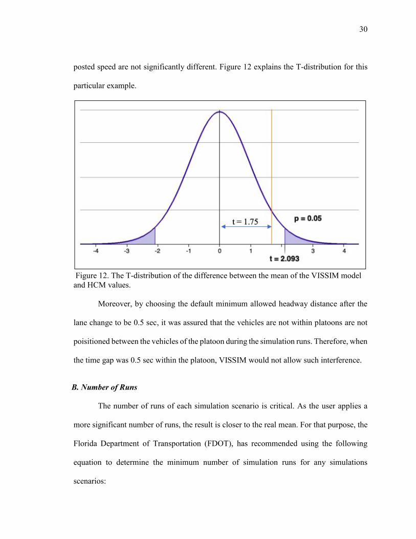
30

posted speed are not significantly different. Figure 12 explains the T-distribution for this

particular example.

Figure 12. The T-distribution of the difference between the mean of the VISSIM model and HCM values.

Moreover, by choosing the default minimum allowed headway distance after the

lane change to be 0.5 sec, it was assured that the vehicles are not within platoons are not

poisitioned between the vehicles of the platoon during the simulation runs. Therefore, when

the time gap was 0.5 sec within the platoon, VISSIM would not allow such interference.

B. Number of Runs

The number of runs of each simulation scenario is critical. As the user applies a

more significant number of runs, the result is closer to the real mean. For that purpose, the

Florida Department of Transportation (FDOT), has recommended using the following

equation to determine the minimum number of simulation runs for any simulations

scenarios:

31

𝒏 = (𝒔×𝒕∝

𝝁×𝜺)𝟐 (7)

Where n is the minimum number of simulation runs, s is the standard deviation of

the simulation runs (based on previous runs), 𝒕∝ is the critical value of the two-sided T-

test with 95% confidence level, µ is the mean of the previously conducted runs, and 𝜀 is

the tolerance error(estimated as 10%). All the simulation runs were conducted using

Equation 7 to ensure a sufficient number of runs. For example, when the capacity was

measured at 70% of HDVs in platoons, it was found that the number of simulations required

was (395×2.09

3165×0.1)2 = 6.81. Therefore, seven simulation runs were used. The minimum

required number of runs was found to be nine, while all the simulations conducted included

20 runs each.

V. Summary

This chapter discussed the operation and the essential factors of HDV platooning systems.

It gave an overview of the software simulations that were used (VISSIM, MOVES, and SSAM)

with some necessary details to understand the foundation of this study. Since the essential part of

the simulation was the VISSIM model, the validity of the model was illustrated by statistical

analysis. It was proven that the VISSIM model does not vary from what the HCM presents. The

next chapter shows the results of the simulation software of HDV’s effect on capacity, greenhouse

emissions, and safety of the hypothetical highway model.

32

CHAPTER 4: HDVS PLATOONING IMPACT ON TRAFFIC FLOW PARAMETERS

This chapter presents the study results. The first and second sections discuss the output of

the simulation scenarios on the model capacity. The third and fourth sections present the effect of

HDVs on greenhouse emissions, with a special focus on carbon dioxide. The effect of HDVs on

highway safety was discussed in the last two sections of this chapter. Each of these sections

presents the output of rigorous analyses that include the ANOVA single factor analysis. In this

study, ANOVA was used to test the effects of various penetration rates on the means of response

variables—capacity, carbon dioxide and conflicts.

I. The Effect of HDVs on Highway Capacity

Many studies have used VISSIM for traffic analysis (Huang, Liu, Yu, & Wang, 2013). The

validity of the hypothetical model was discussed in Chapter 3 of this thesis. The hypothetical model

used in this study has two lanes of 12 feet width. It has the base conditions of a highway as

suggested by HCM. Since VISSIM has some limitations on driving behavior, an External Driver

Module (EDM) was needed to control the desired gaps between vehicles and the drivers’ behavior.

EDM is an interface of VISSIM that provides the option to develop the internal driving behavior

by a full user definition for some or all vehicles in the model. A Dynamic-Link Library (DLL) was

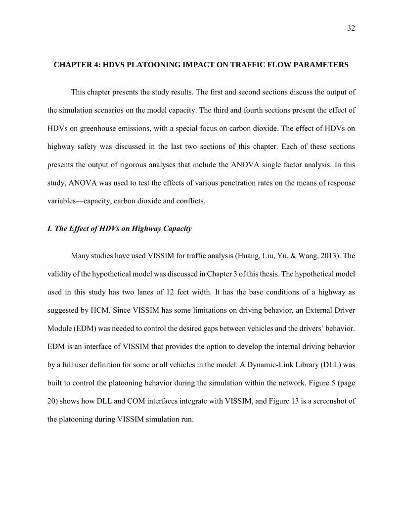
built to control the platooning behavior during the simulation within the network. Figure 5 (page

20) shows how DLL and COM interfaces integrate with VISSIM, and Figure 13 is a screenshot of

the platooning during VISSIM simulation run.

33

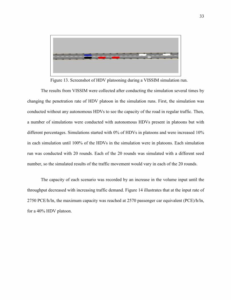
Figure 13. Screenshot of HDV platooning during a VISSIM simulation run.

The results from VISSIM were collected after conducting the simulation several times by

changing the penetration rate of HDV platoon in the simulation runs. First, the simulation was

conducted without any autonomous HDVs to see the capacity of the road in regular traffic. Then,

a number of simulations were conducted with autonomous HDVs present in platoons but with

different percentages. Simulations started with 0% of HDVs in platoons and were increased 10%

in each simulation until 100% of the HDVs in the simulation were in platoons. Each simulation

run was conducted with 20 rounds. Each of the 20 rounds was simulated with a different seed

number, so the simulated results of the traffic movement would vary in each of the 20 rounds.

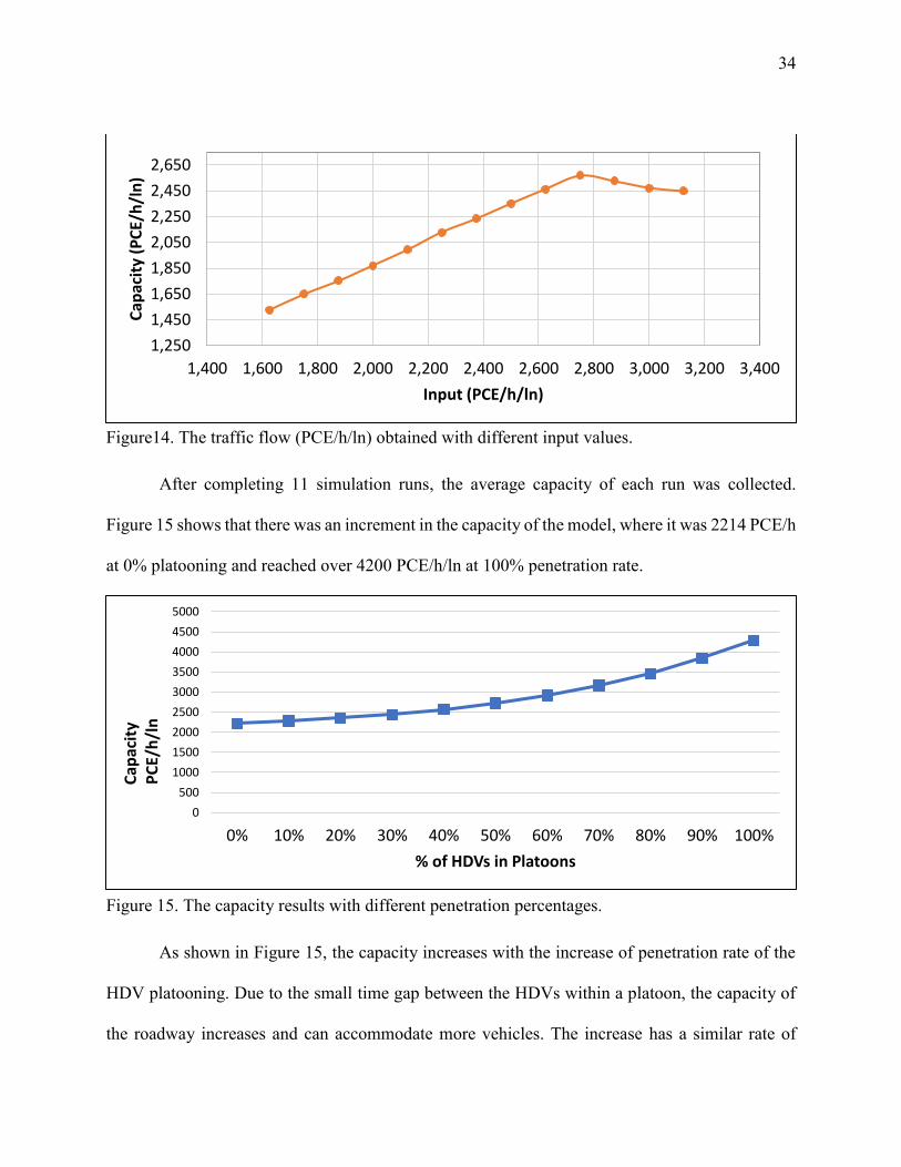
The capacity of each scenario was recorded by an increase in the volume input until the

throughput decreased with increasing traffic demand. Figure 14 illustrates that at the input rate of

2750 PCE/h/ln, the maximum capacity was reached at 2570 passenger car equivalent (PCE)/h/ln,

for a 40% HDV platoon.

34

Figure14. The traffic flow (PCE/h/ln) obtained with different input values.

After completing 11 simulation runs, the average capacity of each run was collected.

Figure 15 shows that there was an increment in the capacity of the model, where it was 2214 PCE/h

at 0% platooning and reached over 4200 PCE/h/ln at 100% penetration rate.

Figure 15. The capacity results with different penetration percentages.

As shown in Figure 15, the capacity increases with the increase of penetration rate of the

HDV platooning. Due to the small time gap between the HDVs within a platoon, the capacity of

the roadway increases and can accommodate more vehicles. The increase has a similar rate of

1,250

1,450

1,650

1,850

2,050

2,250

2,450

2,650

1,400 1,600 1,800 2,000 2,200 2,400 2,600 2,800 3,000 3,200 3,400

Cap

acit

y (P

CE/

h/l

n)

Input (PCE/h/ln)

0

500

1000

1500

2000

2500

3000

3500

4000

4500

5000

0% 10% 20% 30% 40% 50% 60% 70% 80% 90% 100%

Cap

acit

yP

CE/

h/l

n

% of HDVs in Platoons

35

change until 70% penetration of HDVs. A dramatic increase in capacity occurs when the

penetration rate of HDVs in platoons reaches 70%. The percentage of the capacity had increased

to around 8% when the percentage of platooning increases from 60% to 70%, and 8.6% when the

platooning penetration increased another 10% percent to reach 80%. Around 10% of the capacity

had increased when the percentage of platooning reached 90%, likewise at 100%.

This quadratic increment took place since the model started to generate the platoons within

a small amount of time when the penetration rate reached 70%. Thus, individual platoons start to

be closer to each other, and the model asks them to join any autonomous vehicles within short

distance. For that, a number of platoons start to join other platoons which provids more space for

other vehicles to be in the model.

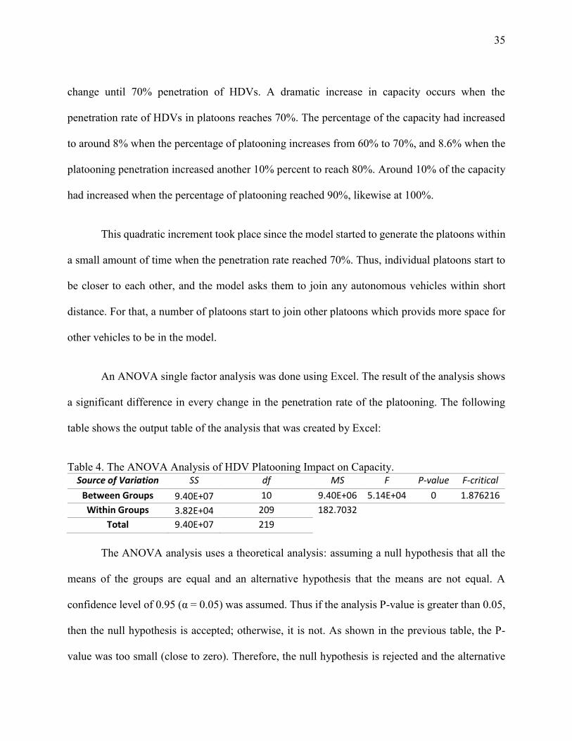
An ANOVA single factor analysis was done using Excel. The result of the analysis shows

a significant difference in every change in the penetration rate of the platooning. The following

table shows the output table of the analysis that was created by Excel:

Table 4. The ANOVA Analysis of HDV Platooning Impact on Capacity. Source of Variation SS df MS F P-value F-critical

Between Groups 9.40E+07 10 9.40E+06 5.14E+04 0 1.876216

Within Groups 3.82E+04 209 182.7032

Total 9.40E+07 219

The ANOVA analysis uses a theoretical analysis: assuming a null hypothesis that all the

means of the groups are equal and an alternative hypothesis that the means are not equal. A

confidence level of 0.95 (α = 0.05) was assumed. Thus if the analysis P-value is greater than 0.05,

then the null hypothesis is accepted; otherwise, it is not. As shown in the previous table, the P-

value was too small (close to zero). Therefore, the null hypothesis is rejected and the alternative

36

hypothesis is accepted, which means there is a significant difference with changing the percentage

of HDV platooning in the capacity of the model.

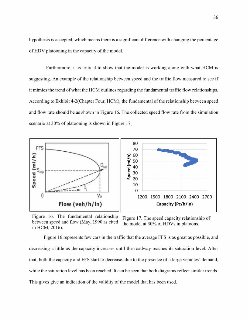
Furthermore, it is critical to show that the model is working along with what HCM is

suggesting. An example of the relationship between speed and the traffic flow measured to see if

it mimics the trend of what the HCM outlines regarding the fundamental traffic flow relationships.

According to Exhibit 4-2(Chapter Four, HCM), the fundamental of the relationship between speed

and flow rate should be as shown in Figure 16. The collected speed flow rate from the simulation

scenario at 30% of platooning is shown in Figure 17.

Figure 16 represents few cars in the traffic that the average FFS is as great as possible, and

decreasing a little as the capacity increases until the roadway reaches its saturation level. After

that, both the capacity and FFS start to decrease, due to the presence of a large vehicles’ demand,

while the saturation level has been reached. It can be seen that both diagrams reflect similar trends.

This gives give an indication of the validity of the model that has been used.

01020304050607080

1200 1500 1800 2100 2400 2700

Spee

d (

mi/

h)

Capacity (Pc/h/ln)

Figure 16. The fundamental relationship between speed and flow (May, 1990 as cited in HCM, 2016).

Figure 17. The speed capacity relationship of the model at 30% of HDVs in platoons.

37

III The Impact Significance of HDV Platoons’ Factors on Capacity

There are many factors involved in the formation and the continuity of every platoon. The most

believed remarkable factors were chosen for as related to the capacity. Each of these factors have

two levels (low and high). The factors included in the study with their levels are as follow:

1. The percentage of trucks in the traffic flow (20%, 80%) and referred to as “Factor A.”

2. The percentage of HDVs which are in platoons to all the HDVs within the traffic flow

(20%, 80%) and referred to as “Factor B.”

3. The time gap between the vehicles in the platoon (0.5 sec, 1.5 sec) and referred to as

“Factor C.”

4. The desired speed of the traffic flow (50 mi/h, 70 mi/h) and referred to as “Factor D.”

5. The number of HDVs in each platoon (3, 5) and referred to as “Factor E.”

The level values for “Factor A” and “Factor B” were chosen to be 20% and 80%, to cover most

of the results of the analysis and also to be close to the tendency of the results. “Factor C” was

chosen based on the minimum gap distance (CACC and ACC) it give to the platoon 0.5 sec and

1.5 sec, respectively. 50 mi/h and 70 mi/h are the low and the high levels for “Factor D,” and were

chosen based on the minimum and maximum speeds on Florida highways. The “Factor E”, the

low level was chosen as the number of HDVs in a platoon in the Energy ITS project, which the

fuel reduction assumption was based on, and the high level was chosen as the length of a

reasonably long platoon.

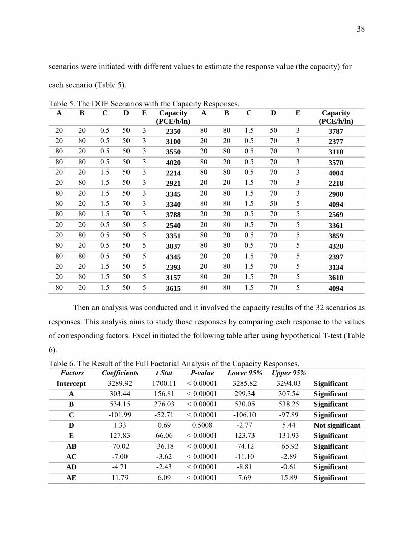
To understand the impact of the platooning factors on the highway capacity, a full factorial

analysis by Excel and Design Of Experiment (DOE) by Minitab were conducted. Thirty-two

38

scenarios were initiated with different values to estimate the response value (the capacity) for

each scenario (Table 5).

Table 5. The DOE Scenarios with the Capacity Responses. A B C D E Capacity

(PCE/h/ln)

A B C D E Capacity

(PCE/h/ln)

20 20 0.5 50 3 2350 80 80 1.5 50 3 3787

20 80 0.5 50 3 3100 20 20 0.5 70 3 2377

80 20 0.5 50 3 3550 20 80 0.5 70 3 3110

80 80 0.5 50 3 4020 80 20 0.5 70 3 3570

20 20 1.5 50 3 2214 80 80 0.5 70 3 4004

20 80 1.5 50 3 2921 20 20 1.5 70 3 2218

80 20 1.5 50 3 3345 20 80 1.5 70 3 2900

80 20 1.5 70 3 3340 80 80 1.5 50 5 4094

80 80 1.5 70 3 3788 20 20 0.5 70 5 2569

20 20 0.5 50 5 2540 20 80 0.5 70 5 3361

20 80 0.5 50 5 3351 80 20 0.5 70 5 3859

80 20 0.5 50 5 3837 80 80 0.5 70 5 4328

80 80 0.5 50 5 4345 20 20 1.5 70 5 2397

20 20 1.5 50 5 2393 20 80 1.5 70 5 3134

20 80 1.5 50 5 3157 80 20 1.5 70 5 3610

80 20 1.5 50 5 3615 80 80 1.5 70 5 4094

Then an analysis was conducted and it involved the capacity results of the 32 scenarios as

responses. This analysis aims to study those responses by comparing each response to the values

of corresponding factors. Excel initiated the following table after using hypothetical T-test (Table

6).

Table 6. The Result of the Full Factorial Analysis of the Capacity Responses. Factors Coefficients t Stat P-value Lower 95% Upper 95%

Intercept 3289.92 1700.11 < 0.00001 3285.82 3294.03 Significant A 303.44 156.81 < 0.00001 299.34 307.54 Significant B 534.15 276.03 < 0.00001 530.05 538.25 Significant C -101.99 -52.71 < 0.00001 -106.10 -97.89 Significant

D 1.33 0.69 0.5008 -2.77 5.44 Not significant

E 127.83 66.06 < 0.00001 123.73 131.93 Significant AB -70.02 -36.18 < 0.00001 -74.12 -65.92 Significant AC -7.00 -3.62 < 0.00001 -11.10 -2.89 Significant AD -4.71 -2.43 < 0.00001 -8.81 -0.61 Significant AE 11.79 6.09 < 0.00001 7.69 15.89 Significant

39

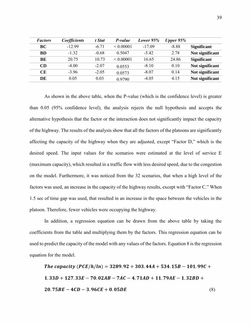
Factors Coefficients t Stat P-value Lower 95% Upper 95%

BC -12.99 -6.71 < 0.00001 -17.09 -8.88 Significant

BD -1.32 -0.68 0.5047 -5.42 2.78 Not significant

BE 20.75 10.73 < 0.00001 16.65 24.86 Significant

CD -4.00 -2.07 0.0553 -8.10 0.10 Not significant

CE -3.96 -2.05 0.0573 -8.07 0.14 Not significant

DE 0.05 0.03 0.9790 -4.05 4.15 Not significant

As shown in the above table, when the P-value (which is the confidence level) is greater

than 0.05 (95% confidence level), the analysis rejects the null hypothesis and accepts the

alternative hypothesis that the factor or the interaction does not significantly impact the capacity

of the highway. The results of the analysis show that all the factors of the platoons are significantly

affecting the capacity of the highway when they are adjusted, except “Factor D,” which is the

desired speed. The input values for the scenarios were estimated at the level of service E

(maximum capacity), which resulted in a traffic flow with less desired speed, due to the congestion

on the model. Furthermore, it was noticed from the 32 scenarios, that when a high level of the

factors was used, an increase in the capacity of the highway results, except with “Factor C.” When

1.5 sec of time gap was used, that resulted in an increase in the space between the vehicles in the

platoon. Therefore, fewer vehicles were occupying the highway.

In addition, a regression equation can be drawn from the above table by taking the

coefficients from the table and multiplying them by the factors. This regression equation can be

used to predict the capacity of the model with any values of the factors. Equation 8 is the regression

equation for the model.

𝑻𝒉𝒆 𝒄𝒂𝒑𝒂𝒄𝒊𝒕𝒚 (𝑷𝑪𝑬/𝒉/𝒍𝒏) = 𝟑𝟐𝟖𝟗. 𝟗𝟐 + 𝟑𝟎𝟑. 𝟒𝟒𝑨 + 𝟓𝟑𝟒. 𝟏𝟓𝑩 − 𝟏𝟎𝟏. 𝟗𝟗𝑪 +

𝟏. 𝟑𝟑𝑫 + 𝟏𝟐𝟕. 𝟑𝟑𝑬 − 𝟕𝟎. 𝟎𝟐𝑨𝑩 − 𝟕𝑨𝑪 − 𝟒. 𝟕𝟏𝑨𝑫 + 𝟏𝟏. 𝟕𝟗𝑨𝑬 − 𝟏. 𝟑𝟐𝑩𝑫 +

𝟐𝟎. 𝟕𝟓𝑩𝑬 − 𝟒𝑪𝑫 − 𝟑. 𝟗𝟔𝑪𝑬 + 𝟎. 𝟎𝟓𝑫𝑬 (8)

40

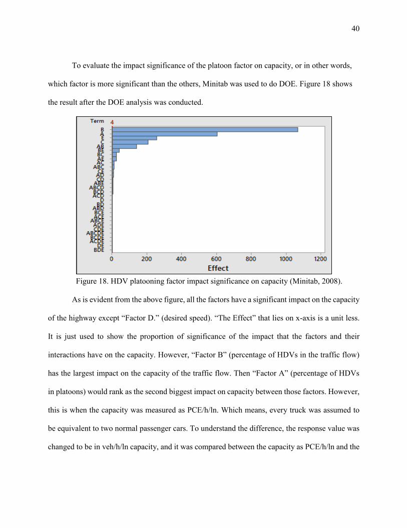
To evaluate the impact significance of the platoon factor on capacity, or in other words,

which factor is more significant than the others, Minitab was used to do DOE. Figure 18 shows

the result after the DOE analysis was conducted.

Figure 18. HDV platooning factor impact significance on capacity (Minitab, 2008).

As is evident from the above figure, all the factors have a significant impact on the capacity

of the highway except “Factor D.” (desired speed). “The Effect” that lies on x-axis is a unit less.

It is just used to show the proportion of significance of the impact that the factors and their

interactions have on the capacity. However, “Factor B” (percentage of HDVs in the traffic flow)

has the largest impact on the capacity of the traffic flow. Then “Factor A” (percentage of HDVs

in platoons) would rank as the second biggest impact on capacity between those factors. However,

this is when the capacity was measured as PCE/h/ln. Which means, every truck was assumed to

be equivalent to two normal passenger cars. To understand the difference, the response value was

changed to be in veh/h/ln capacity, and it was compared between the capacity as PCE/h/ln and the

41

capacity as veh/h/ln. The two figures (19-A & 19-B) show the actual impact of the “Factor A” and

“Factor B.” on the capacity.

A

B

Figure19. Contour plot of “Factor A”, and “Factor B“ VS. A- capacity as (PCE/h/ln), and B-capacity as (veh/h/ln).

Inter-distance 1

Desire Speed 60

No. of HDVs 4

Hold Values

Factor B

Fact

or A

80706050403020

80

70

60

50

40

30

20

>

–

–

–

–

–

–

< 2500

2500 2750

2750 3000

3000 3250

3250 3500

3500 3750

3750 4000

4000

(PCE/h/ln)

Capacity

Inter-distance 1

Desire Speed 60

No. of HDVs 4

Hold Values

Factor B

Fact

or A

80706050403020

80

70

60

50

40

30

20

>

–

–

–

–

–

–

< 2000

2000 2100

2100 2200

2200 2300

2300 2400

2400 2500

2500 2600

2600

(Veh/h/ln)

Capacity

% of HDVs in platoons

% of HDVs in platoons

% o

f HD

Vs i

n tra

ffic

flow

%

of H

DV

s in

traffi

c flo

w

42

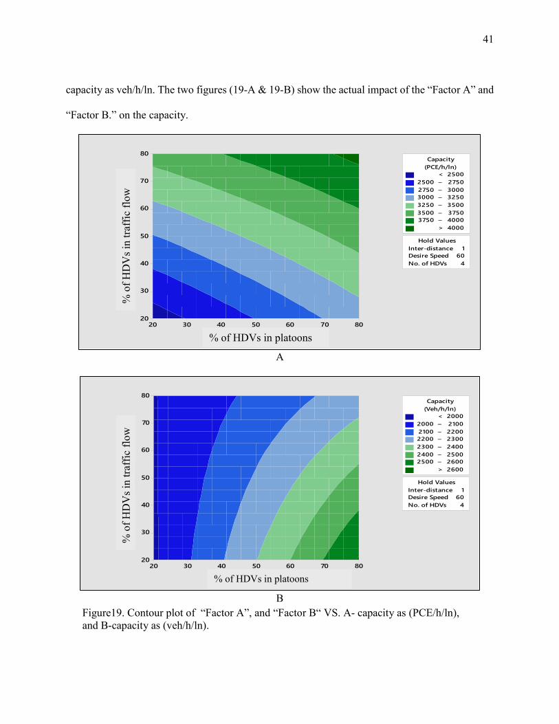
As evident from the two figures above, the increase in the percentage of trucks in the traffic

flow would increase the capacity as PCE if it is assumed to be equivalent to two passenger cars.

However, in the matter of the number of vehicles that can pass through the traffic model,

increasing the amount of vehicles in traffic would decrease the capacity.

III. The Effect of HDVs on Highway Greenhouse Emissions

This experiment runs on MOVES was chosen to be an on-road model with project domain.

According to FHWA, 26% of the gas emissions within the United States is CO2, and 90% of that

comes from transportation sectors (Schmitt, & Sprung, 2011). Hence, CO2 was chosen as the

primary greenhouse gas emission rate for the same 11 scenarios as in the capacity study. Since the

hypothetical model has similar characteristics to I-295 highway, the county of Duval in

Jacksonville was chosen to have the default values for the meteorology data and other necessary

input values. Either the input values into MOVES were taken from VISSIM simulation runs or the

default data given by EPA for the chosen county. It is worth mentioning that in the fuel tab, the

fuel usage fraction template was used to estimate the fuel reduction in the platoons according to

what the ITS Energy study suggested (Figure 2, page 13). After fulfillment of the MOVES

navigation panel and CDM tabs, a simulation run was conducted on MOVES for all the scenarios.

The database given in the summary report cannot be changed or added to get the total emissions

without using MYSQL. With the help of MYSQL, it was possible to analyze and calculate the

total CO2 emission, and the total energy consumed for all the scenarios, export ingthe results in

Excel tables. The following figure shows the CO2 emission from MYSQL files for the different

penetration percentages of HDVs in the platoons:

43

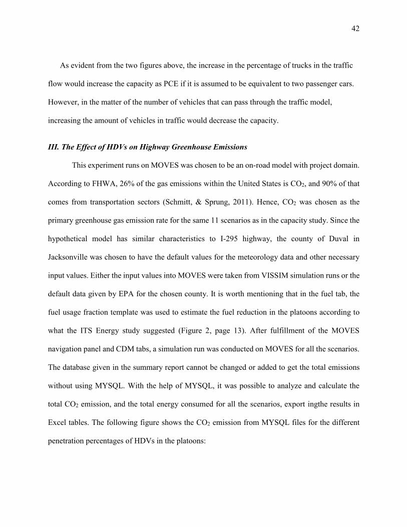
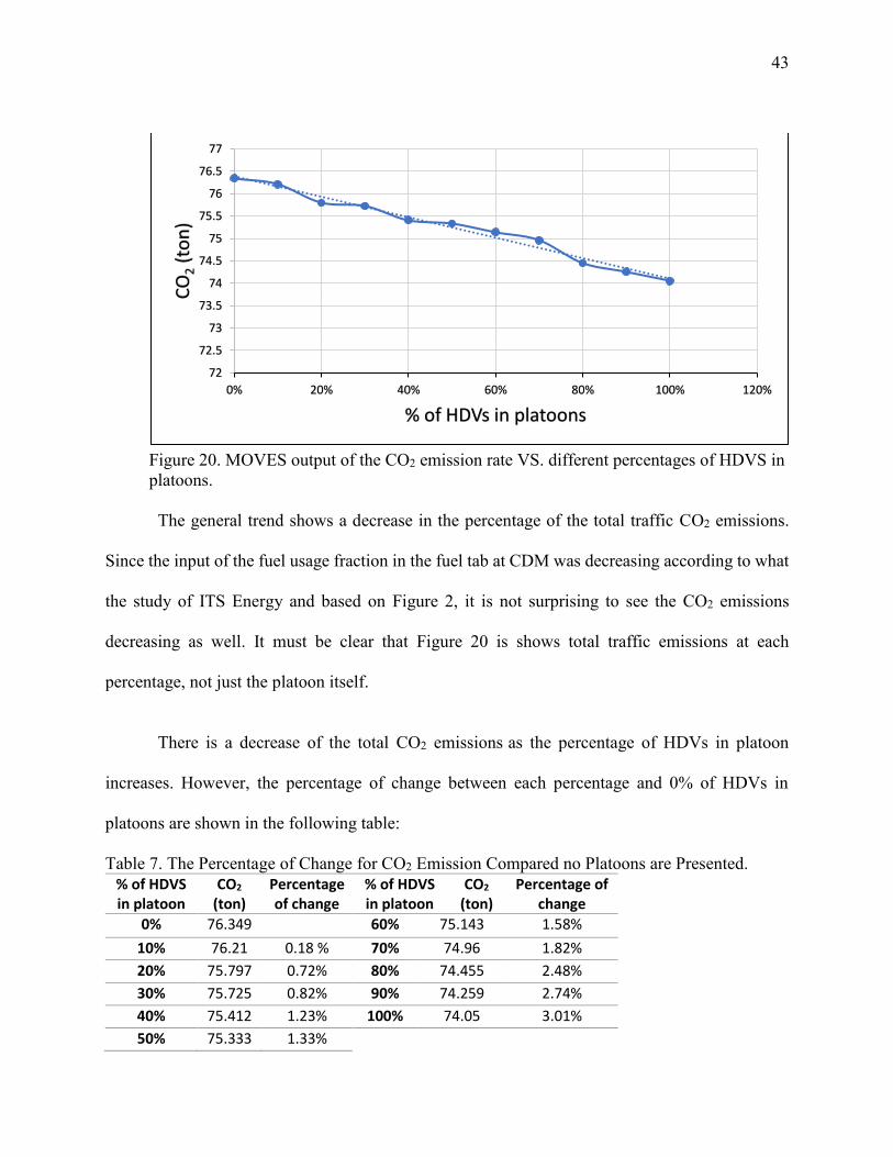
Figure 20. MOVES output of the CO2 emission rate VS. different percentages of HDVS in platoons.

The general trend shows a decrease in the percentage of the total traffic CO2 emissions.

Since the input of the fuel usage fraction in the fuel tab at CDM was decreasing according to what

the study of ITS Energy and based on Figure 2, it is not surprising to see the CO2 emissions

decreasing as well. It must be clear that Figure 20 is shows total traffic emissions at each

percentage, not just the platoon itself.

There is a decrease of the total CO2 emissions as the percentage of HDVs in platoon

increases. However, the percentage of change between each percentage and 0% of HDVs in

platoons are shown in the following table:

Table 7. The Percentage of Change for CO2 Emission Compared no Platoons are Presented. % of HDVS in platoon

CO2 (ton)

Percentage of change

% of HDVS in platoon

CO2 (ton)

Percentage of change

0% 76.349

60% 75.143 1.58%

10% 76.21 0.18 % 70% 74.96 1.82%

20% 75.797 0.72% 80% 74.455 2.48%

30% 75.725 0.82% 90% 74.259 2.74%

40% 75.412 1.23% 100% 74.05 3.01%

50% 75.333 1.33%

72

72.5

73

73.5

74

74.5

75

75.5

76

76.5

77

0% 20% 40% 60% 80% 100% 120%

CO

2(t

on

)

% of HDVs in platoons

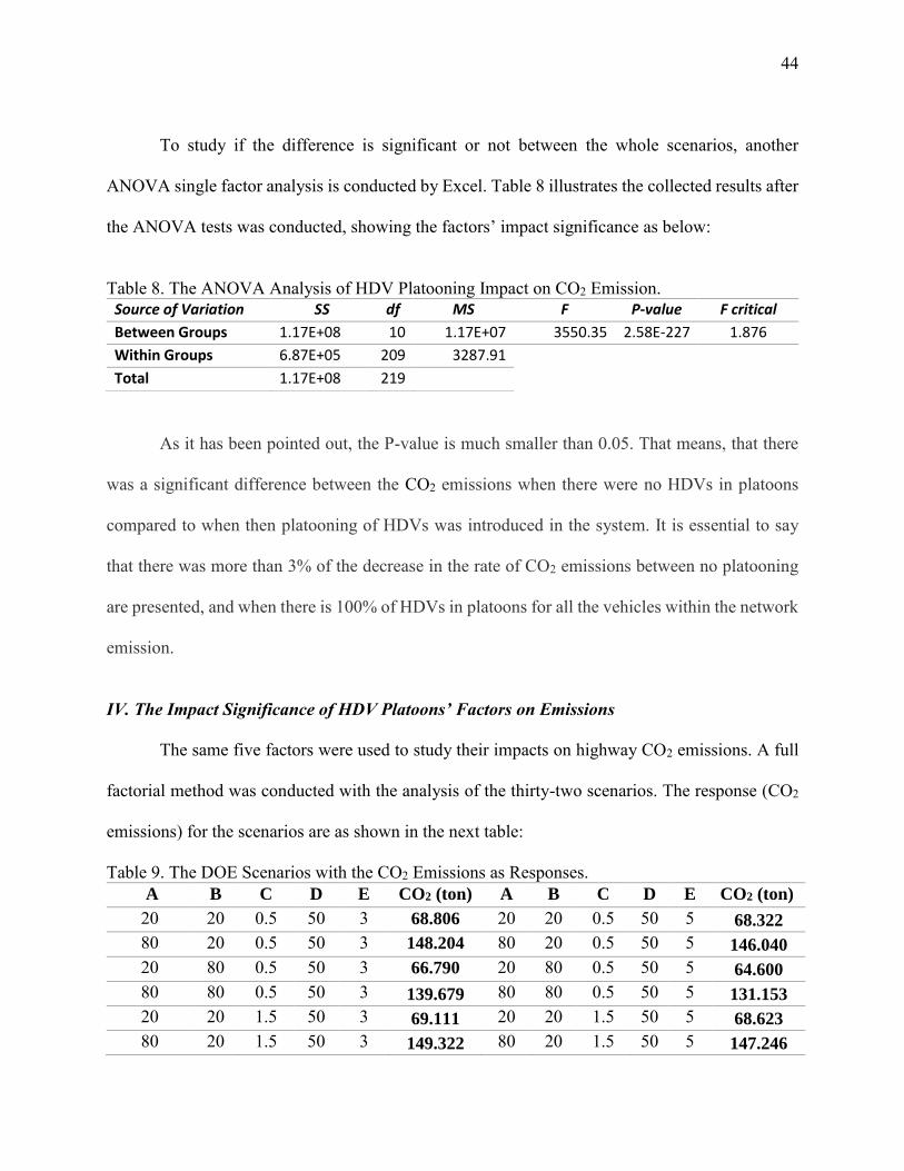
44

To study if the difference is significant or not between the whole scenarios, another

ANOVA single factor analysis is conducted by Excel. Table 8 illustrates the collected results after

the ANOVA tests was conducted, showing the factors’ impact significance as below:

Table 8. The ANOVA Analysis of HDV Platooning Impact on CO2 Emission.

As it has been pointed out, the P-value is much smaller than 0.05. That means, that there

was a significant difference between the CO2 emissions when there were no HDVs in platoons

compared to when then platooning of HDVs was introduced in the system. It is essential to say

that there was more than 3% of the decrease in the rate of CO2 emissions between no platooning

are presented, and when there is 100% of HDVs in platoons for all the vehicles within the network

emission.

IV. The Impact Significance of HDV Platoons’ Factors on Emissions

The same five factors were used to study their impacts on highway CO2 emissions. A full

factorial method was conducted with the analysis of the thirty-two scenarios. The response (CO2

emissions) for the scenarios are as shown in the next table:

Table 9. The DOE Scenarios with the CO2 Emissions as Responses.

Source of Variation SS df MS F P-value F critical

Between Groups 1.17E+08 10 1.17E+07 3550.35 2.58E-227 1.876

Within Groups 6.87E+05 209 3287.91

Total 1.17E+08 219

A B C D E CO2 (ton) A B C D E CO2 (ton)

20 20 0.5 50 3 68.806 20 20 0.5 50 5 68.322

80 20 0.5 50 3 148.204 80 20 0.5 50 5 146.040

20 80 0.5 50 3 66.790 20 80 0.5 50 5 64.600

80 80 0.5 50 3 139.679 80 80 0.5 50 5 131.153

20 20 1.5 50 3 69.111 20 20 1.5 50 5 68.623

80 20 1.5 50 3 149.322 80 20 1.5 50 5 147.246

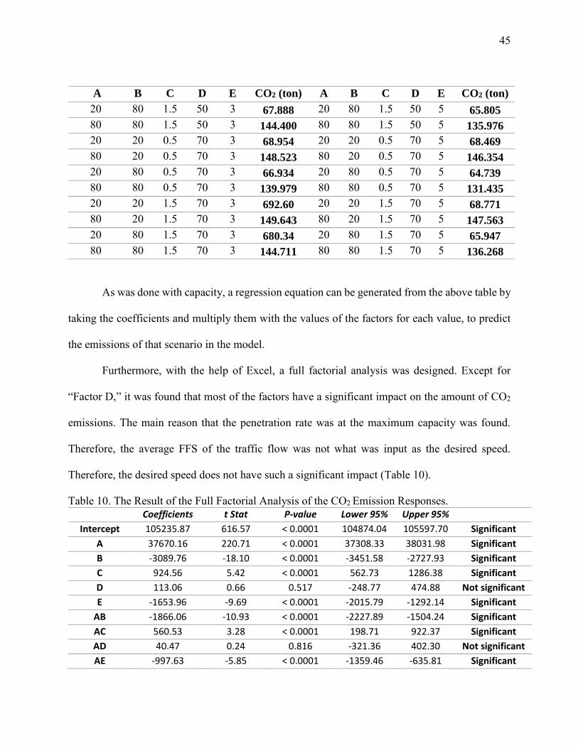
45

As was done with capacity, a regression equation can be generated from the above table by

taking the coefficients and multiply them with the values of the factors for each value, to predict

the emissions of that scenario in the model.

Furthermore, with the help of Excel, a full factorial analysis was designed. Except for

“Factor D,” it was found that most of the factors have a significant impact on the amount of CO2

emissions. The main reason that the penetration rate was at the maximum capacity was found.

Therefore, the average FFS of the traffic flow was not what was input as the desired speed.

Therefore, the desired speed does not have such a significant impact (Table 10).

Table 10. The Result of the Full Factorial Analysis of the CO2 Emission Responses. Coefficients t Stat P-value Lower 95% Upper 95%

Intercept 105235.87 616.57 < 0.0001 104874.04 105597.70 Significant

A 37670.16 220.71 < 0.0001 37308.33 38031.98 Significant

B -3089.76 -18.10 < 0.0001 -3451.58 -2727.93 Significant

C 924.56 5.42 < 0.0001 562.73 1286.38 Significant

D 113.06 0.66 0.517 -248.77 474.88 Not significant

E -1653.96 -9.69 < 0.0001 -2015.79 -1292.14 Significant

AB -1866.06 -10.93 < 0.0001 -2227.89 -1504.24 Significant

AC 560.53 3.28 < 0.0001 198.71 922.37 Significant

AD 40.47 0.24 0.816 -321.36 402.30 Not significant

AE -997.63 -5.85 < 0.0001 -1359.46 -635.81 Significant

A B C D E CO2 (ton) A B C D E CO2 (ton)

20 80 1.5 50 3 67.888 20 80 1.5 50 5 65.805

80 80 1.5 50 3 144.400 80 80 1.5 50 5 135.976

20 20 0.5 70 3 68.954 20 20 0.5 70 5 68.469

80 20 0.5 70 3 148.523 80 20 0.5 70 5 146.354

20 80 0.5 70 3 66.934 20 80 0.5 70 5 64.739

80 80 0.5 70 3 139.979 80 80 0.5 70 5 131.435

20 20 1.5 70 3 692.60 20 20 1.5 70 5 68.771

80 20 1.5 70 3 149.643 80 20 1.5 70 5 147.563

20 80 1.5 70 3 680.34 20 80 1.5 70 5 65.947

80 80 1.5 70 3 144.711 80 80 1.5 70 5 136.268

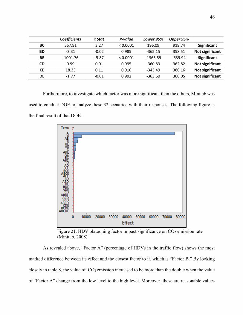
46

Coefficients t Stat P-value Lower 95% Upper 95%

BC 557.91 3.27 < 0.0001 196.09 919.74 Significant

BD -3.31 -0.02 0.985 -365.15 358.51 Not significant

BE -1001.76 -5.87 < 0.0001 -1363.59 -639.94 Significant

CD 0.99 0.01 0.995 -360.83 362.82 Not significant

CE 18.33 0.11 0.916 -343.49 380.16 Not significant

DE -1.77 -0.01 0.992 -363.60 360.05 Not significant

Furthermore, to investigate which factor was more significant than the others, Minitab was

used to conduct DOE to analyze these 32 scenarios with their responses. The following figure is

the final result of that DOE.

Figure 21. HDV platooning factor impact significance on CO2 emission rate (Minitab, 2008)

As revealed above, “Factor A” (percentage of HDVs in the traffic flow) shows the most

marked difference between its effect and the closest factor to it, which is “Factor B.” By looking

closely in table 8, the value of CO2 emission increased to be more than the double when the value

of “Factor A” change from the low level to the high level. Moreover, these are reasonable values

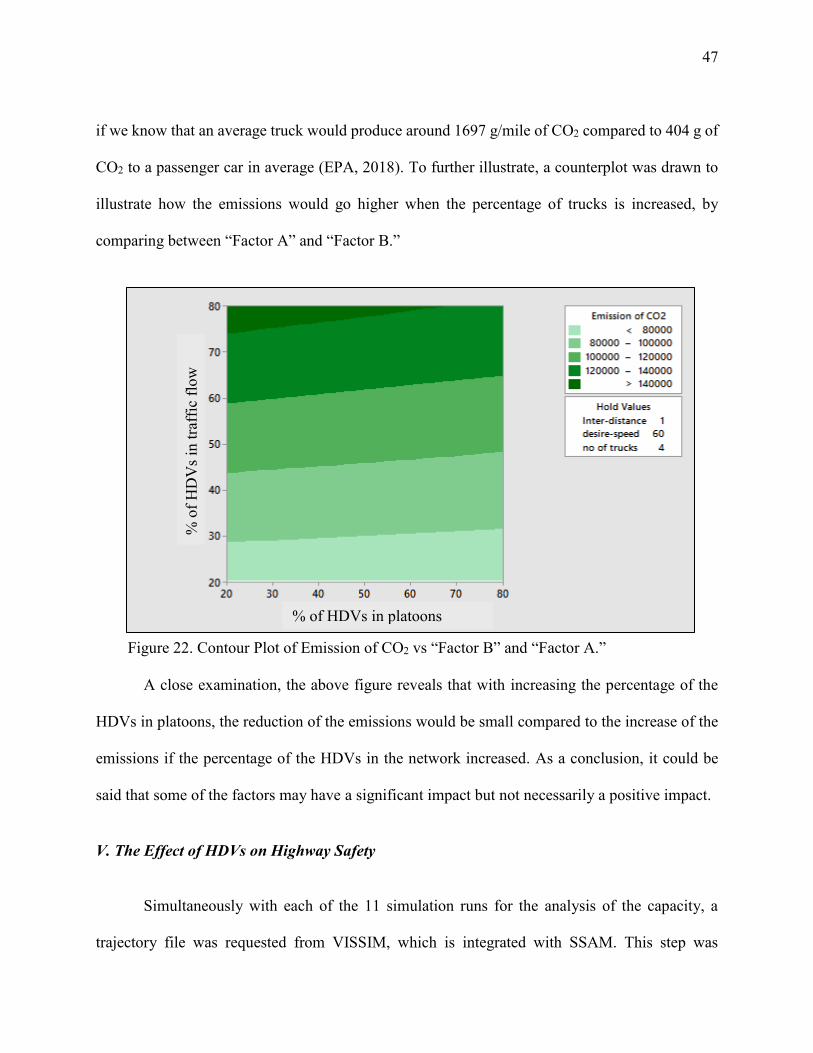
47

if we know that an average truck would produce around 1697 g/mile of CO2 compared to 404 g of

CO2 to a passenger car in average (EPA, 2018). To further illustrate, a counterplot was drawn to

illustrate how the emissions would go higher when the percentage of trucks is increased, by

comparing between “Factor A” and “Factor B.”

Figure 22. Contour Plot of Emission of CO2 vs “Factor B” and “Factor A.”

A close examination, the above figure reveals that with increasing the percentage of the

HDVs in platoons, the reduction of the emissions would be small compared to the increase of the

emissions if the percentage of the HDVs in the network increased. As a conclusion, it could be

said that some of the factors may have a significant impact but not necessarily a positive impact.

V. The Effect of HDVs on Highway Safety

Simultaneously with each of the 11 simulation runs for the analysis of the capacity, a

trajectory file was requested from VISSIM, which is integrated with SSAM. This step was

% of HDVs in platoons

% o

f HD

Vs i

n tra

ffic

flow

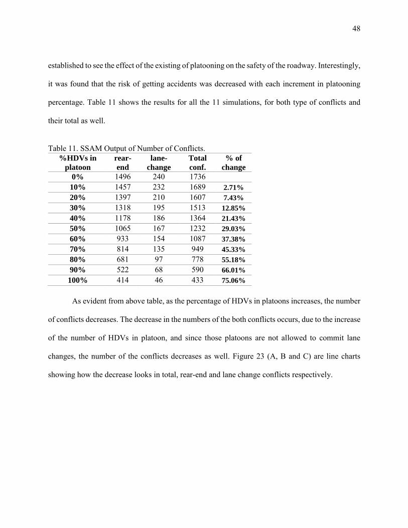
48

established to see the effect of the existing of platooning on the safety of the roadway. Interestingly,

it was found that the risk of getting accidents was decreased with each increment in platooning

percentage. Table 11 shows the results for all the 11 simulations, for both type of conflicts and

their total as well.

Table 11. SSAM Output of Number of Conflicts. %HDVs in

platoon

rear-

end

lane-

change

Total

conf.

% of

change

0% 1496 240 1736 10% 1457 232 1689 2.71%

20% 1397 210 1607 7.43%

30% 1318 195 1513 12.85%

40% 1178 186 1364 21.43%

50% 1065 167 1232 29.03%

60% 933 154 1087 37.38%

70% 814 135 949 45.33%

80% 681 97 778 55.18%

90% 522 68 590 66.01%

100% 414 46 433 75.06%

As evident from above table, as the percentage of HDVs in platoons increases, the number

of conflicts decreases. The decrease in the numbers of the both conflicts occurs, due to the increase

of the number of HDVs in platoon, and since those platoons are not allowed to commit lane

changes, the number of the conflicts decreases as well. Figure 23 (A, B and C) are line charts

showing how the decrease looks in total, rear-end and lane change conflicts respectively.

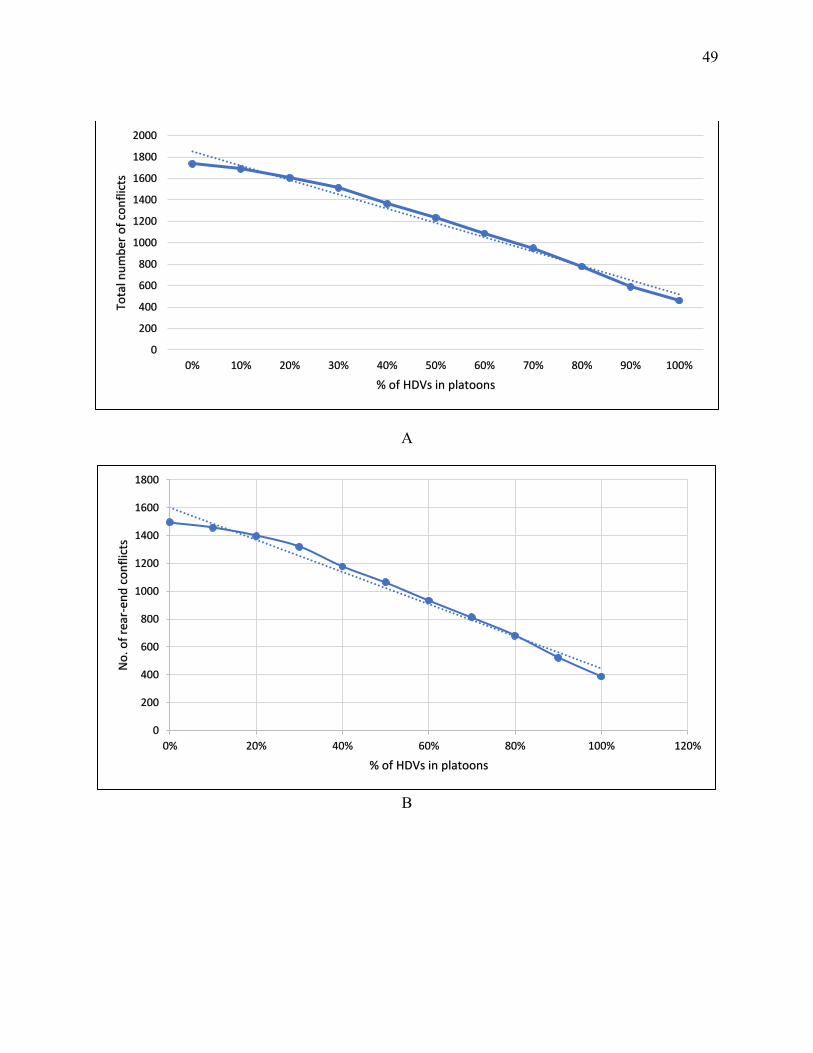
49

A

B

0

200

400

600

800

1000

1200

1400

1600

1800

2000

0% 10% 20% 30% 40% 50% 60% 70% 80% 90% 100%

Tota

l nu

mb

er o

f co

nfl

icts

% of HDVs in platoons

0

200

400

600

800

1000

1200

1400

1600

1800

0% 20% 40% 60% 80% 100% 120%

No

. of

rear

-en

d c

on

flic

ts

% of HDVs in platoons

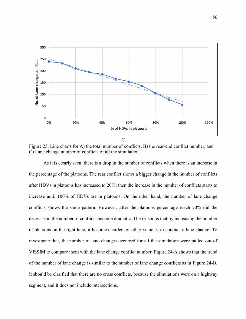
50

C

Figure 23. Line charts for A) the total number of conflicts, B) the rear-end conflict number, and C) Lane change number of conflicts of all the simulation.

As it is clearly seen, there is a drop in the number of conflicts when there is an increase in

the percentage of the platoons. The rear conflict shows a bigger change in the number of conflicts

after HDVs in platoons has increased to 20%: then the increase in the number of conflicts starts to

increase until 100% of HDVs are in platoons. On the other hand, the number of lane change

conflicts shows the same pattern. However, after the platoons percentage reach 70% did the

decrease in the number of conflicts become dramatic. The reason is that by increasing the number

of platoons on the right lane, it becomes harder for other vehicles to conduct a lane change. To

investigate that, the number of lane changes occurred for all the simulation were pulled out of

VISSIM to compare them with the lane change conflict number. Figure 24-A shows that the trend

of the number of lane change is similar to the number of lane change conflicts as in Figure 24-B.

It should be clarified that there are no cross conflicts, because the simulations were on a highway

segment, and it does not include intersections.

0

50

100

150

200

250

300

0% 20% 40% 60% 80% 100% 120%

No

. of

Lan

e ch

ange

co

nfl

icts

% of HDVs in platoons

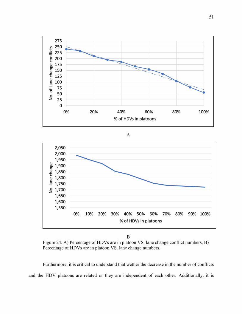
51

A

B Figure 24. A) Percentage of HDVs are in platoon VS. lane change conflict numbers, B) Percentage of HDVs are in platoon VS. lane change numbers.

Furthermore, it is critical to understand that wether the decrease in the number of conflicts

and the HDV platoons are related or they are independent of each other. Additionally, it is

0255075

100125150175200225250275

0% 20% 40% 60% 80% 100%

No

. of

Lan

e ch

ange

co

nfl

icts

% of HDVs in platoons

1,550

1,600

1,650

1,700

1,750

1,800

1,850

1,900

1,950

2,000

2,050

0% 10% 20% 30% 40% 50% 60% 70% 80% 90% 100%

No

. lan

e ch

ange

% of HDVs in platoons

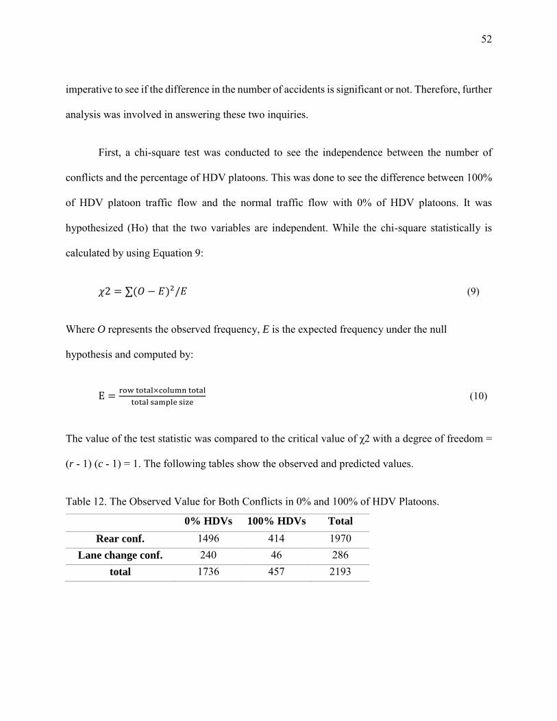
52

imperative to see if the difference in the number of accidents is significant or not. Therefore, further

analysis was involved in answering these two inquiries.

First, a chi-square test was conducted to see the independence between the number of

conflicts and the percentage of HDV platoons. This was done to see the difference between 100%

of HDV platoon traffic flow and the normal traffic flow with 0% of HDV platoons. It was

hypothesized (Ho) that the two variables are independent. While the chi-square statistically is

calculated by using Equation 9:

𝜒2 = ∑(𝑂 − 𝐸)2/𝐸 (9)

Where O represents the observed frequency, E is the expected frequency under the null

hypothesis and computed by:

E =row total×column total

total sample size (10)

The value of the test statistic was compared to the critical value of χ2 with a degree of freedom =

(r - 1) (c - 1) = 1. The following tables show the observed and predicted values.

Table 12. The Observed Value for Both Conflicts in 0% and 100% of HDV Platoons.

0% HDVs 100% HDVs Total

Rear conf. 1496 414 1970 Lane change conf. 240 46 286

total 1736 457 2193

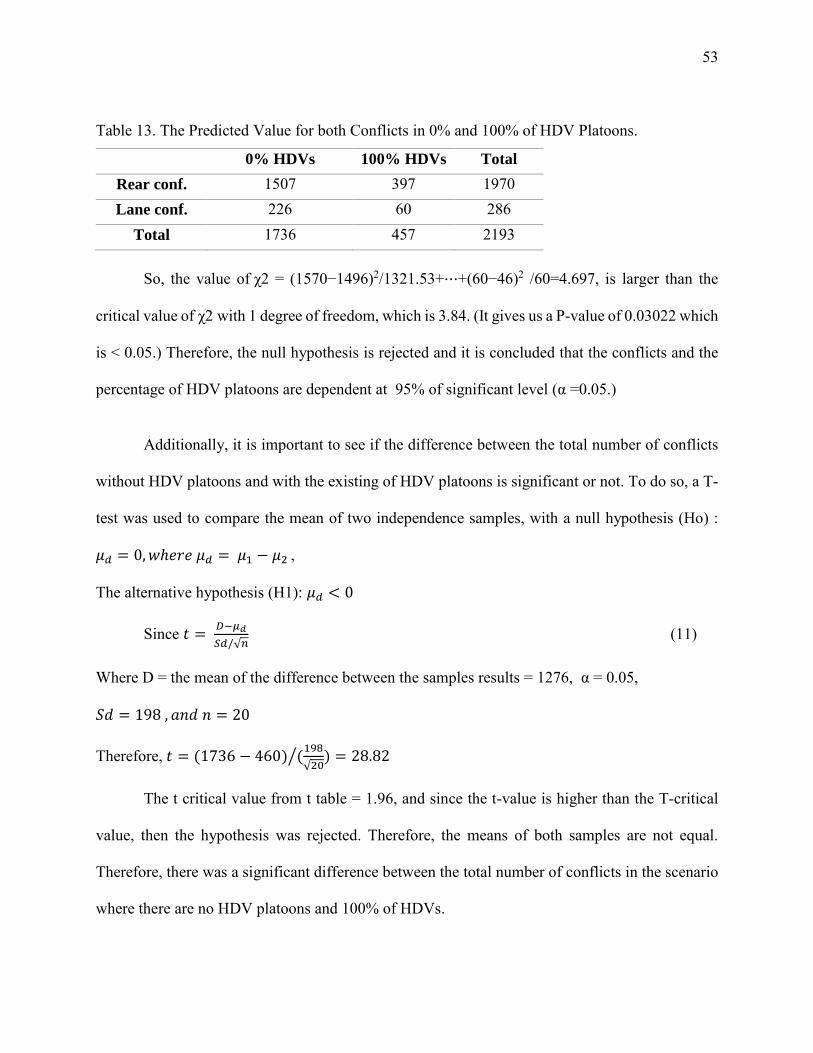
53

Table 13. The Predicted Value for both Conflicts in 0% and 100% of HDV Platoons.

0% HDVs 100% HDVs Total

Rear conf. 1507 397 1970 Lane conf. 226 60 286

Total 1736 457 2193

So, the value of χ2 = (1570−1496)2/1321.53+⋯+(60−46)2 /60=4.697, is larger than the

critical value of χ2 with 1 degree of freedom, which is 3.84. (It gives us a P-value of 0.03022 which

is < 0.05.) Therefore, the null hypothesis is rejected and it is concluded that the conflicts and the

percentage of HDV platoons are dependent at 95% of significant level (α =0.05.)

Additionally, it is important to see if the difference between the total number of conflicts

without HDV platoons and with the existing of HDV platoons is significant or not. To do so, a T-

test was used to compare the mean of two independence samples, with a null hypothesis (Ho) :

𝜇𝑑 = 0, 𝑤ℎ𝑒𝑟𝑒 𝜇𝑑 = 𝜇1 − 𝜇2 ,

The alternative hypothesis (H1): 𝜇𝑑 < 0

Since 𝑡 = 𝐷−𝜇𝑑

𝑆𝑑/√𝑛 (11)

Where D = the mean of the difference between the samples results = 1276, α = 0.05,

𝑆𝑑 = 198 , 𝑎𝑛𝑑 𝑛 = 20

Therefore, 𝑡 = (1736 − 460) (198

√20)⁄ = 28.82

The t critical value from t table = 1.96, and since the t-value is higher than the T-critical

value, then the hypothesis was rejected. Therefore, the means of both samples are not equal.

Therefore, there was a significant difference between the total number of conflicts in the scenario

where there are no HDV platoons and 100% of HDVs.

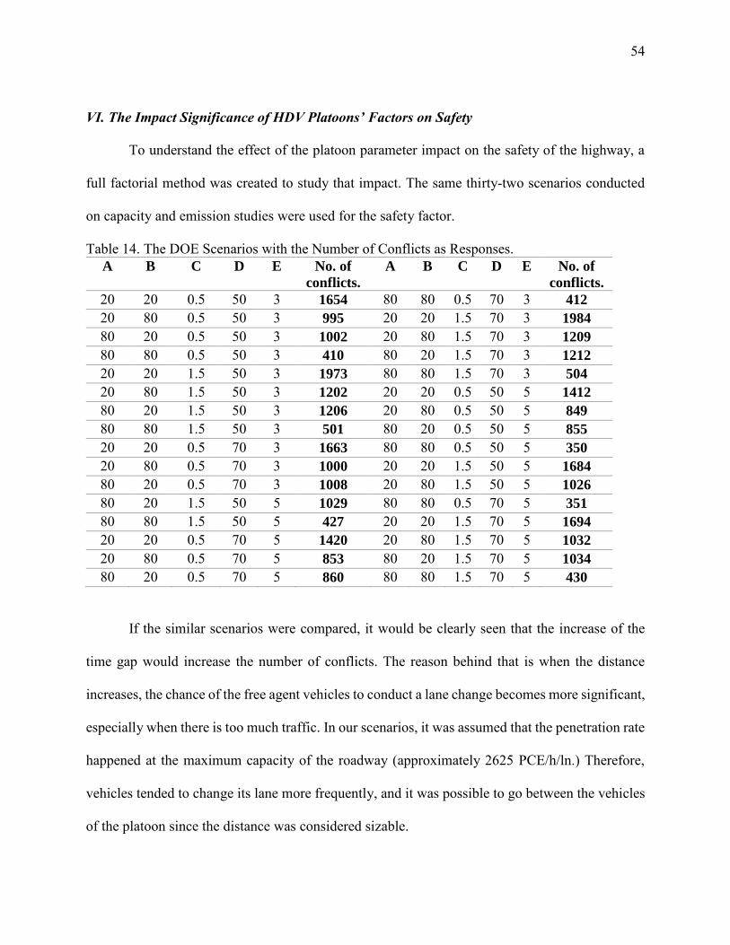
54

VI. The Impact Significance of HDV Platoons’ Factors on Safety

To understand the effect of the platoon parameter impact on the safety of the highway, a

full factorial method was created to study that impact. The same thirty-two scenarios conducted

on capacity and emission studies were used for the safety factor.

Table 14. The DOE Scenarios with the Number of Conflicts as Responses. A B C D E No. of

conflicts.

A B C D E No. of

conflicts.

20 20 0.5 50 3 1654 80 80 0.5 70 3 412

20 80 0.5 50 3 995 20 20 1.5 70 3 1984

80 20 0.5 50 3 1002 20 80 1.5 70 3 1209

80 80 0.5 50 3 410 80 20 1.5 70 3 1212

20 20 1.5 50 3 1973 80 80 1.5 70 3 504

20 80 1.5 50 3 1202 20 20 0.5 50 5 1412

80 20 1.5 50 3 1206 20 80 0.5 50 5 849

80 80 1.5 50 3 501 80 20 0.5 50 5 855

20 20 0.5 70 3 1663 80 80 0.5 50 5 350

20 80 0.5 70 3 1000 20 20 1.5 50 5 1684

80 20 0.5 70 3 1008 20 80 1.5 50 5 1026

80 20 1.5 50 5 1029 80 80 0.5 70 5 351

80 80 1.5 50 5 427 20 20 1.5 70 5 1694

20 20 0.5 70 5 1420 20 80 1.5 70 5 1032

20 80 0.5 70 5 853 80 20 1.5 70 5 1034

80 20 0.5 70 5 860 80 80 1.5 70 5 430

If the similar scenarios were compared, it would be clearly seen that the increase of the

time gap would increase the number of conflicts. The reason behind that is when the distance

increases, the chance of the free agent vehicles to conduct a lane change becomes more significant,

especially when there is too much traffic. In our scenarios, it was assumed that the penetration rate

happened at the maximum capacity of the roadway (approximately 2625 PCE/h/ln.) Therefore,

vehicles tended to change its lane more frequently, and it was possible to go between the vehicles

of the platoon since the distance was considered sizable.

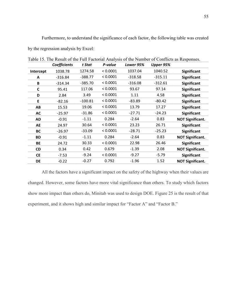
55

Furthermore, to understand the significance of each factor, the following table was created

by the regression analysis by Excel:

Table 15. The Result of the Full Factorial Analysis of the Number of Conflicts as Responses. Coefficients t Stat P-value Lower 95% Upper 95%

Intercept 1038.78 1274.58 < 0.0001 1037.04 1040.52 Significant

A -316.84 -388.77 < 0.0001 -318.58 -315.11 Significant

B -314.34 -385.70 < 0.0001 -316.08 -312.61 Significant

C 95.41 117.06 < 0.0001 93.67 97.14 Significant

D 2.84 3.49 < 0.0001 1.11 4.58 Significant

E -82.16 -100.81 < 0.0001 -83.89 -80.42 Significant

AB 15.53 19.06 < 0.0001 13.79 17.27 Significant

AC -25.97 -31.86 < 0.0001 -27.71 -24.23 Significant

AD -0.91 -1.11 0.284 -2.64 0.83 NOT Significant.

AE 24.97 30.64 < 0.0001 23.23 26.71 Significant

BC -26.97 -33.09 < 0.0001 -28.71 -25.23 Significant

BD -0.91 -1.11 0.284 -2.64 0.83 NOT Significant.

BE 24.72 30.33 < 0.0001 22.98 26.46 Significant

CD 0.34 0.42 0.679 -1.39 2.08 NOT Significant.

CE -7.53 -9.24 < 0.0001 -9.27 -5.79 Significant

DE -0.22 -0.27 0.792 -1.96 1.52 NOT Significant.

All the factors have a significant impact on the safety of the highway when their values are

changed. However, some factors have more vital significance than others. To study which factors

show more impact than others do, Minitab was used to design DOE. Figure 25 is the result of that

experiment, and it shows high and similar impact for “Factor A” and “Factor B.”

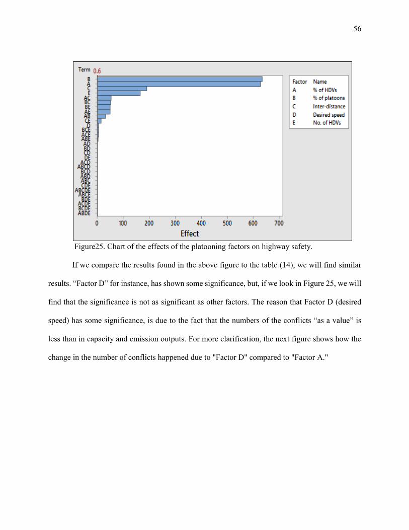
56

Figure25. Chart of the effects of the platooning factors on highway safety. If we compare the results found in the above figure to the table (14), we will find similar

results. “Factor D” for instance, has shown some significance, but, if we look in Figure 25, we will

find that the significance is not as significant as other factors. The reason that Factor D (desired

speed) has some significance, is due to the fact that the numbers of the conflicts “as a value” is

less than in capacity and emission outputs. For more clarification, the next figure shows how the

change in the number of conflicts happened due to "Factor D" compared to "Factor A."

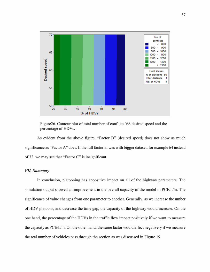
57

Figure26. Contour plot of total number of conflicts VS desired speed and the percentage of HDVs.

As evident from the above figure, “Factor D” (desired speed) does not show as much

significance as “Factor A” does. If the full factorial was with bigger dataset, for example 64 instead

of 32, we may see that “Factor C” is insignificant.

VII. Summary

In conclusion, platooning has appositive impact on all of the highway parameters. The

simulation output showed an improvement in the overall capacity of the model in PCE/h/ln. The

significance of value changes from one parameter to another. Generally, as we increase the umber

of HDV platoons, and decrease the time gap, the capacity of the highway would increase. On the

one hand, the percentage of the HDVs in the traffic flow impact positively if we want to measure

the capacity as PCE/h/ln. On the other hand, the same factor would affect negatively if we measure

the real number of vehicles pass through the section as was discussed in Figure 19.

58

Furthermore, 100% of HDV platooning would decrease the emissions rate of the overall

traffic emissions about 3% when comparing if there were not any platooning on the traffic. This is

mainly based on the consumption reduction in the HDVs platoons when the HDVs are driven in

such a close distance. The increase in “Factor C” would negatively affect and increase the CO2

emission.

Moreover, the penetration of HDV platoons decreases the number of conflicts in highway

traffic, as the output of SSAM suggests. Since the distance between the vehicles of the platoons is

such a small distance (0.5 sec), the lane change number decreases. That leads to a decrease in the

number of lane change conflicts. Also, the number of penetration in the scenarios is the same, and

with increasing the number of HDVs in platoons, the possibility of rear-end conflicts decreases.

However, with increasing the distance between the vehicles in the platoon, the free agent vehicles

tend to perform a lane change between the vehicles of the platoon, which increase the number of

lane changes as well.

59

Chapter 5: OVERALL SUMMARY AND RECOMMENDATIONS

This study is based on a hypothetical model that was created by VISSIM software. This

model was the backbone of this study and its output. The model was considered to have the

characteristics of the base condition highway corresponding to what HCM suggests. Different

statistical methods investigated the validity of this model and compared it the expected values of

HCM. In addition to VISSIM, MOVES, and SSAM are two simulation software packages that

used to obtain the CO2 emissions and the safety results, respectively. These two software packages

are dependent on the model created by VISSIM.

To investigate the effect of the platoon’s factors effect, a full factorial method was created,

after conducting thirty-two simulation scenarios. The factors were chosen to be: A) The percentage

of HDVs in the traffic flow; B) The percentage of platoons; C) The time gap; D) The desired speed

of the traffic flow; E) The number of HDVs in every single platoon.

By the end of this study, it was found that as the percentage of HDVs in platoon increased,

the highway parameters would be positively affected. Furthermore, increasing the number of HDV

in platoons, the highway traffic parameters would be enhanced is discussed with details in Chapter

4. Additionally, most of the chosen platoon factors have a significant impact on the highway

parameters, except for the desired speed due to the high penetration rate used.

It is worth to mentioning that most of the studies conducted on platooning, have been

mostly concerned with the reduction of fuel consumption, which has been considered the main

idea behind the creation of platoons in the first place. This thesis focuses mainly on the effect of

the HDV platooning on the highway parameters. In addition, it investigates the impact that those

platoons’ factors have on the parameters. As was mentioned, this thesis was based on a verified

hypothetical model. Several assumptions were involved for the simplicity and clarification

60

purposes. However, it was recommended that future work be done in the conduction of similar

study using a real highway data as an input. In addition, the limitation of the model could be

reduced to enhance the model results.

61

REFERENCES

Al Alam, A. (2011). Fuel-efficient distributed control for heavy duty vehicle platooning.

VETENSKAP OCH KONST school. Retrieved from http://www.diva-

portal.org/smash/record.jsf?pid=diva2:447050

Archer, J. (2005). Indicators for traffic safety assessment and prediction and their application in

micro-simulation modelling: A study of urban and suburban intersections. Thesis, Royal

Institute of Technology, Department of Infrastructure, Division for Transport and Logistics,

Centre for Transport Research. Retrieved from https://doi.org/ISBN 91-7323-119-3

Browand, F., McArthur, J., & Radovich, C. (2004). Fuel saving achieved in the field test of two

tandem trucks california PATH research report. [Research Report]. Retrieved from

http://its.berkeley.edu/sites/default/files/publications/UCB/2004/PRR/UCB-ITS-PRR-2004-

20.pdf

Caudill, R. J., & Garrard, W. L. (2010). Vehicle-Follower Longitudinal Control for Automated

Transit Vehicles. Journal of Dynamic Systems, Measurement, and Control, 99(4), 241.

Retrieved from https://doi.org/10.1115/1.3427114

Davis, L. C. (2004). Effect of adaptive cruise control systems on traffic flow. Physical Review E

- Statistical Physics, Plasmas, Fluids, and Related Interdisciplinary Topics, 69(6), 8.

Retrieved from https://doi.org/10.1103/PhysRevE.69.066110

Envirnomintal Protection Egency (EPA). (2018). Fast facts: U.S. transportation sector

greenhouse gas emissions, 1990-2016 (EPA-420-F-18-013, July 2018). Retrieved from

https://nepis.epa.gov/Exe/ZyPDF.cgi?Dockey=P100USI5.pdf

62

Farah, H., Koutsopoulos, H. N., Saifuzzaman, M., Kölbl, R., Fuchs, S., & Bankosegger, D.

(2012). Evaluation of the effect of cooperative infrastructure-to-vehicle systems on driver

behavior. Transportation Research Part C: Emerging Technologies, 21(1), 42–56. Retrieved

from https://doi.org/10.1016/j.trc.2011.08.006

Florida Department of Transportation (FDOT). (2019). Online Sunshine. Retrieved from

http://www.leg.state.fl.us/

Garrard, W. L. (1979). Model-follower longitudinal control for automated guideway transit

vehicles. IEEE Transactions on Vehicular Technology, 28(1), 36–45. Retrieved from

https://doi.org/10.1109/T-VT.1979.23768

Hall, C. T., & Noel, G. J. (2014). The Usage of the U . S . Environmental Protection Agency ’ s (

USEPA ) Motor Vehicle Emission Simulator ( MOVES ) with the Federal Aviation

Administration ’ s ( FAA ) Emissions and Dispersion Modeling System ( EDMS ), (March).

Retrieved from

https://www.epa.gov/sites/production/files/201503/documents/2013_dqrs_certified.pdf

Huang, F., Liu, P., Yu, H., & Wang, W. (2013). Identifying if VISSIM simulation model and

SSAM provide reasonable estimates for field measured traffic conflicts at signalized

intersections. Accident Analysis and Prevention, 50, 1014–1024. Retrieved from

https://doi.org/10.1016/j.aap.2012.08.018

Lehmann, A. (2010, August). Graph and set alerts on MySQL performance, plus data from the

rest of your apps + infrastructure. Retrieved from https://www.quora.com/What-is-MySQL-

used-for-and-what-are-its-advantages-and-disadvantages

Liang, K. Y., Martensson, J., & Johansson, K. H. (2013). When is it fuel eficient for a heavy

duty vehicle to catch up with a platoon? IFAC Proceedings Volumes (IFAC-PapersOnline),

7(PART), 738–743. Retrieved from https://doi.org/10.3182/20130904-4-JP-2042.00071

63

Liang, K. Y., Mårtensson, J., & Johansson, K. H. (2016). Heavy-Duty Vehicle Platoon

Formation for Fuel Efficiency. IEEE Transactions on Intelligent Transportation Systems,

17(4), 1051–1061. Retrieved from https://doi.org/10.1109/TITS.2015.2492243

May, A. (1990). Traffic Flow Fundamentals. [text] Retrieved from

http://docshare02.docshare.tips/files/25341/253416450.pdf

Mesa-Arango, R., & Fabregas A. (2017). Impacts of automated truck platoons on travel time and

reliability at freeway diverge areas. Transportation Research Board.

Minderhoud, M. M., & Bovy, P. H. L. (2001). Extended time-to-collision measures for road

traffic safety assessment. Accident Analysis and Prevention, 33(1), 89–97. Retrieved from

https://doi.org/10.1016/S0001-4575(00)00019-1

Nadimi, N., Behbahani, H., & Shahbazi, H. R. (2016). Calibration and validation of a new time-

based surrogate safety measure using fuzzy inference system. Journal of Traffic and

Transportation Engineering, 3(1), 51–58. Retrieved from

https://doi.org/10.1016/j.jtte.2015.09.004

Peng, Y., Abdel-Aty, M., Shi, Q., & Yu, R. (Revised 2017). Assessing the impact of reduced

visibility on traffic crash risk using microscopic data and surrogate safety measures.

Transportation Research Part C: Emerging Technologies, 74(January 2008), 295–305.

Retrieved from https://doi.org/10.1016/j.trc.2016.11.022

Ploeg, J., Scheepers, B. T. M., Van Nunen, E., Van De Wouw, N., & Nijmeijer, H. (2011).

Design and experimental evaluation of cooperative adaptive cruise control. IEEE

Conference on Intelligent Transportation Systems, Proceedings, ITSC, 260–265. Retrieved

from https://doi.org/10.1109/ITSC.2011.6082981

64

Saffarzadeh, M., Nadimi, N., Naseralavi, S., & Mamdoohi, A. R. (2012). A general formulation

for time-to-collision safety indicator. Proceedings of the Institution of Civil Engineers -

Transport, 166(5), 294–304. Retrieved from https://doi.org/10.1680/tran.11.00031

Schmitt, R. & Sprung, M. (2011). Fright facts and figures. US. Departmentof Transportation.

Retrieved from

https://ops.fhwa.dot.gov/freight/freight_analysis/nat_freight_stats/docs/11factsfigures/pdfs/f

ff2011_highres.pdf

Shladover, S. E., Desoer, C. A., Hedrick, J. K., Tomizuka, M., Walrand, J., Member, S., …

Mckeown, N. (1991). Shladover et al. - 1991 - Automatic Vehicle Control Developments in

the PATH Program.pdf, 40(1). Retrieved from

http://yuba.stanford.edu/~nickm/papers/00069979.pdf

Transportation Research Board. (2016). Chapter 12: Highway Capacity Manual. Retrieved from

https://doi.org/10.1061/(ASCE)HY.1943-7900.0000746.

Tsugawa, S. (2009). A Survey on Effects of ITS –related Systems and Technologies on Global

Warming Prevention. 12th IFAC symosiom on transportation system, Rebondo Beach, CA,

Septemper 2-4, 2009. Retrieved from https://doi.org/10.3182/20090902-3-US-2007.0084

Tsugawa, S. (2013). An overview on an automated truck platoon within the energy ITS project.

IFAC Proceedings Volumes (IFAC-PapersOnline) (Vol. 7). IFAC. Retrieved from

https://doi.org/10.3182/20130904-4-JP-2042.00110

Tsugawa, S. (2014). Results and issues of an automated truck platoon within the energy ITS

project. IEEE Intelligent Vehicles Symposium. Retrieved from

https://doi.org/10.1109/IVS.2014.6856400

65

Tsugawa, S., Jeschke, S., & Shladover, S. E. (2016). A review of truck platooning projects for

energy savings. IEEE Transactions on Intelligent Vehicles, 1(1), 68–77. Retrieved from

https://doi.org/10.1109/TIV.2016.2577499

Vahidi, A., & Eskandarian, A. (2003). Research advances in intelligent collision avoidance and

adaptive cruise control. IEEE Transactions on Intelligent Transportation Systems, 4(3),

143–153. Retrieved from

https://pdfs.semanticscholar.org/dfbb/9078d75d41e3a58ab06e64d876d76b1b1970.pdf

Van Arem, B., Van Driel, C. J. G., & Visser, R. (2006). The impact of cooperative adaptive

cruise control on traffic-flow characteristics. IEEE Transactions on Intelligent

Transportation Systems, 7(4), 429–436. Retrieved from

https://doi.org/10.1109/TITS.2006.884615

Van Nunen, E., Esposto, F., Saberi, A. K., & Paardekooper, J. P. (2017). Evaluation of safety

indicators for truck platooning. In IEEE Intelligent Vehicles Symposium. Retrieved from

https://doi.org/10.1109/IVS.2017.7995847

Zwaneveld, P., & van Arem, B. (1998). Traffic effects of automated vehicle guidance systems.

Proceedings ITS World Congress, (15), Delft, The Netherland, Retrieved from

https://pdfs.semanticscholar.org/e2a6/96da7cc8a614d5a3a4c8f84c4f523a45048a.pdf

Zhao, L., & Sun, J. (2013). Simulation Framework for Vehicle Platooning and Car-following

Behaviors Under Connected-vehicle Environment. Procedia - Social and Behavioral

Sciences, 96(Cictp), 914–924. Retrieved from https://doi.org/10.1016/j.sbspro.2013.08.105

66

VITAE

AHMED ALZAHRANI

Objective

Joining an extraordinary university to expand my knowledge in transportation engineering and to explore,

discover and develop significant contributions to my career and the transportation sector.

Education and Training

University of North Florida | Jacksonville, FL

Master of Science in Transportation Engineering

2019

Currently enrolled with 3.71 as a GPA

Major in Transportation Engineering

Thesis: The Effect of Truck Platooning on Highway Parameters.

A Member of Institute of Transportation Engineers (ITE)

King Abdul Aziz university | Jeddah

Bachelor of Science in Civil Engineering

2013

Graduated at 2013 with 3.312 of GPA

Saudi Society of Civil Engineering (SSCE) Member

Experience

University of North Florida |

Jacksonville, FL

Graduate Student

08/2017 - Current

Attended in- Conferences, workshops, and Participation: had the

chance to attend TRB in Washington D.C. in 2019, the FSIT

conference that was held in Fort Lauderdale in 2018, the Florida

Automated Vehicle summits in 2017 and 2018.

A participant with a paper at the Florida Automated Vehicle

Summit 2018, entitled “Truck Platooning Effect on Highway

Parameters.”

King Abdul Aziz University | Jeddah,

Makkah

Teaching Assistant

04/2014 - 08/2016

Teaching Experience: worked as a teaching assistant at KAU and

was responsible for developing lesson plans, lectures, problem

sets, and final exam questions, as well as the syllabus for a new

degree program. Collaborated with teacher to devise and

implement developmentally appropriate lessons aligning with

school's philosophy and mission.

67

Saudi Electricity Company (National

Grid) | Jeddah, Makkah

Field Engineer

01/2014 - 08/2014

Worked as a site and quality control engineer. My main duty was

the supervision on the construction of electricity stations and its

safety.

Hired and supervised subcontractors to improve production and

ensure safety requirements were met.

Certifications

AutoCAD certification with Grade (Very good) from KAU.

Certified from American Concrete Institute (ACI), as concrete field-testing technician grade 1.

English language program graduate at UNF

Skills

Professionalism in transportation software such

VISSIM and MOVES.

Professionalism in SoliedWork, AutoCAD and

STAADPro, software.

The ability of teaching, tutoring and counseling.

Good experience in communication skills.

Summery

Reliable graduate student eager to prove himself as a transportation engineer. With his experience in

teaching and research, his aspiration and goals are limitless to have an impact in transportation sector.