The Origins of Firm Heterogeneity: AProduction Network Approach∗

Andrew B. Bernard† Emmanuel Dhyne‡ Glenn Magerman§

Kalina Manova¶ Andreas Moxnes‖

May 2021

Abstract

This paper explores firm size heterogeneity in production networks. Using all buyer-supplier relationships in Belgium, the paper shows that firms with more customers havehigher total sales but lower sales per customer and lower market shares among thosecustomers. A decomposition of firm sales reveals that downstream factors, especiallythe number of customers, explain the large majority of firm size heterogeneity. Thesefacts motivate a model of heterogeneous firms and network formation where firms searchfor and sell to downstream buyers and buy inputs from upstream suppliers. Firms varyin their productivity and relationship capability. Higher productivity results in morematches and larger market shares among customers. Higher relationship capability re-sults in more customers and higher sales. Estimated model parameters suggest thatproductivity and relationship capability are strongly negatively correlated. A counter-factual exercise shows that the real wage gains from improving relationship capabilityare substantial, and much larger in our model compared to canonical models of one-dimensional heterogeneity.

∗This project has received funding from the European Research Council (ERC) under the EuropeanUnion’s Horizon 2020 research and innovation programme (grant agreements No 715147 and No 724880).The views expressed here are those of the authors and do not necessarily reflect those of the National Bankof Belgium. We thank the editor, five anonymous referees, discussants Julian di Giovanni, Isabelle Mejean,Jasmine Xiao and Thomas Åstebro, aand numerousseminar participants for helpful comments and valuablediscussion.

†Tuck School of Business at Dartmouth, CEP, CEPR & NBER; andrew.b.bernard@tuck.dartmouth.edu‡National Bank of Belgium & Université de Mons; Emmanuel.Dhyne@nbb.be§ECARES - Université libre de Bruxelles, CEPR & National Bank of Belgium; glenn.magerman@ulb.be¶University College London, CEPR & CEP; k.manova@ucl.ac.uk‖University of Oslo & CEPR; andreamo@econ.uio.no

1

JEL: D24, F10, F12, F16, L11, L25

Keywords: Firm size heterogeneity, productivity, relationship capability, productionnetwork, network formation, matching costs.

1 Introduction

Even within narrowly defined industries, there is massive dispersion in firm outcomes suchas sales, employment and productivity. In Belgium, a firm at the 90th percentile of thesize distribution has turnover 32 times greater than a firm at the 10th percentile withinthe same industry.1 Understanding the origins of firm size heterogeneity is a fundamentalquestion in economics and has important micro- and macroeconomic implications. At themicro level, bigger firms perform systematically better along many dimensions, includingsurvival, innovation, and participation in international trade (e.g., Bernard et al., 2012). Atthe macro level, the skewness and granularity of the firm size distribution affect aggregateproductivity, the welfare gains from trade, and the impact of idiosyncratic and systemicshocks (e.g., Pavcnik, 2002, Gabaix, 2011, di Giovanni et al., 2014, Melitz and Redding,2015 and Gaubert and Itskhoki, 2021).

This paper examines the firm size distribution in a production network with firm hetero-geneity and buyer-supplier connections.2 The basic premise of the analysis is intuitive: firmscan be large because (i) they have inherently attractive capabilities such as productivity orquality, (ii) they have low marginal costs from matches with more or better suppliers, and/or(iii) they have higher sales due to more or bigger buyers. Higher-order effects can also beimportant, as the customers of customers also ultimately affect firm economic outcomes.

While research has made progress in identifying underlying firm-specific supply- anddemand-side factors driving firm size (e.g., Hottman et al., 2016), much less is known aboutthe role of buyer-seller linkages in production networks. In particular, the focus on the supplyside has been on heterogeneity in either firm productivity (e.g., Jovanovic, 1982, Hopenhayn,1992, Melitz, 2003, Luttmer, 2007) or organizational capital (e.g., Prescott and Visscher,1980, Luttmer, 2011), whereas work on the demand side has centered on final customerpreferences (e.g., Fitzgerald et al., 2016) or firm-specific demand shocks (e.g. Foster et al.,2016). To the extent that the literature has considered firm-to-firm trade, it has typicallyremained anchored in one-sided heterogeneity by assuming that firms source inputs fromanonymous upstream suppliers or sell to anonymous downstream buyers, without accountingfor the heterogeneity of all trade partners in the production network.

Our contribution is threefold. First, we document new stylized facts about productionnetworks using data on the universe of firm-to-firm domestic transactions in Belgium, and1 The p90/p10 ratio is averaged across all NACE 4-digit Belgian industries in 2014. Hottman et al. (2016)

report even larger sales dispersion across firms using barcode data on US retail sales, and Autor et al.(2020)find that 52.6 percent of sales in the average US industry is accounted for by the 20 largest firms,representing less than half a percent of the total number of firms.

2 Throughout the paper, firm size refers to sales or turnover, and we use both terms interchangeably.

1

present the first extensive analysis of how upstream, downstream and final demand hetero-geneity translate into firm size heterogeneity. Second, we provide a theoretical frameworkfor an endogenous production network with firm heterogeneity in both productivity/qualityand relationship capability. Third, we estimate the parameters of the model using simu-lated method of moments to explore the relative importance of the two dimensions of firmheterogeneity and their interaction across firms.

We report three stylized facts from the production network data that motivate the sub-sequent analysis and model. First, the distributions of total sales and buyer-supplier con-nections exhibit high dispersion. The enormous dispersion of sales across firms is also foundin the production network in terms of the number of links to buyers and suppliers. Second,firms with more customers have higher sales but lower average sales per customer and lowermarket shares (shares of input purchases) among their customers. Finally, there is negativedegree assortativity between buyers and suppliers: sellers with more customers match withcustomers who have fewer suppliers on average.

Taken together, these facts both confirm intuition and challenge existing models of firmheterogeneity. The large variation in sales across firms within an industry is intuitivelyrelated to variation in the number of customers: large firms have more customers. However,firms with more customers have lower average sales per customer, connect with less well-connected customers, and account for a smaller share of those customers’ input purchases.Models that emphasize heterogeneity in productivity across firms cannot explain all threefacts simultaneously. In particular, such models imply that firms with more customers shouldalso sell more to each of their customers: they should have larger, not smaller market shares.

A key advantage of the Belgian production network data is that sales from firm i to jcan be decomposed into seller-, buyer- and match-specific components.3 This allows us tounderstand how much of the value of pairwise sales is due to the seller, the buyer or the matchitself. High dispersion in seller effects means that firms vary in how much they sell to theircustomers, controlling for demand by those customers, i.e. firms differ in their average marketshare across customers. Conversely, high dispersion in buyer effects means that some firmsmatch with large customers while others do not, leading to larger sales even as the averagemarket share remains the same. Given estimates of these fixed effects, the total sales of afirm can be decomposed into three distinct factors: (i) an upstream component that capturesthe firm’s ability to obtain large market shares across its customers, (ii) a downstreamcomponent that captures the firm’s ability to attract many and/or large customers, and (iii)a final demand component that captures the firm’s ability to sell relatively more outside the3 Our approach is similar to the inter-temporal analysis of matched employer-employee data (e.g. Abowd

et al., 1999).

2

domestic network, to final consumers at home or to foreign customers.The results are striking: 81 percent of the variation in firm sales within narrowly defined

(4-digit NACE) industries is associated with the downstream component, while the upstreamcomponent contributes only 18 percent. The variation in firm size is largely unrelated to therelative importance of sales to final demand (1 percent). These findings imply that trade inintermediate goods and the number of firm-to-firm connections are essential to understandingfirm performance and, consequently, aggregate outcomes.

Motivated by these stylized facts and decomposition results, we develop a quantitativegeneral equilibrium model of firm-to-firm trade. In the model, firms use a constant-elasticity-of-substitution production technology that combines labor and inputs from upstream sup-pliers. Firms sell their output to final consumers and to domestic producers. Firms differin two dimensions – productivity and relationship capability – defined respectively as pro-duction efficiency and (the inverse of) the fixed cost of matching with a customer. The twodimensions are potentially correlated. Suppliers match with customers if the gross profitsof the match exceed the supplier-specific fixed matching cost. Marginal costs, employment,prices, and sales are endogenous outcomes because they depend on the outcomes of all otherfirms in the economy. A link between two firms increases the total sales of both the sellerand the buyer; for the seller this occurs mechanically because it gains a customer, while forthe buyer this arises because a larger supplier base lowers the marginal cost of production.

The model equilibrium involves three nested fixed points. A backward fixed point deter-mines the price of a firm as a function of its marginal cost, which in turn depends on theprices of its suppliers. A forward fixed point pins down the sales of a firm as a function ofdemand by its customers, which in turn depends on their sales to their customers. A linkfunction fixed point relates the likelihood of a link to the profit from the match, which isitself a function of the network structure. Jointly, these determine the endogenous structureof the network in terms of connections, the value of bilateral sales for each link, and the totalsales of the firm.

We estimate the model parameters using simulated method of moments. These parame-ters comprise the variance of productivity, the mean and variance of relationship capability,and the correlation between productivity and relationship capability across firms. The resultsreveal high dispersion in relationship capability across firms and a strong negative correlationbetween the two firm characteristics. Firms with higher productivity have lower relationshipcapability. This negative relationship is crucial for matching the stylized fact that firmswith more customers have lower average sales per customer and lower market share in thosecustomers. A canonical model without this negative relationship instead produces a stronglypositive relationship between the number of customers and average sales (or average market

3

share). The model does well at matching untargeted moments, such as the variances oftotal sales and value added. In addition, it does well at matching moments on the upstreamside of the production network, including the variances of the number of suppliers and totalinput purchases. Importantly, both dimensions of firm heterogeneity are necessary to matchthe data: shutting down one at a time results in poor model fit, including the inability toreplicate the negative relationship between the number of customers and average sales percustomer.

Why are the two dimensions of firm capabilities negatively related? While it is outside thescope of this paper to offer a fully specified explanation, a possible answer is imperfect rewardand incentive systems. For example, Holmstrom and Milgrom (1991) offer a multitaskingtheory where agents will focus their effort on observable and rewarded tasks at the expenseof other tasks. If the principal only rewards one dimension of performance, e.g. findingcustomers, this might reduce other dimensions of firm performance, such as product qualityor productivity.4

Finally, we use the estimated model to quantify the role of firm heterogeneity in produc-tivity and relationship capability for aggregate outcomes. Specifically, we cut relationshipcosts across all firms by 50 percent. We do so in two versions of our model; in the baselineestimated model and then in a restricted model with no correlation between productivity andrelationship costs. The counterfactual reveals that the real wage gains from lowering rela-tionship costs are substantial, and much larger in our baseline model compared to the modelwith no correlation structure. The reason is that the fall in relationship costs benefits thehigh-productivity firms relatively more in the baseline model, as they are more constrainedby high relationship costs.

This paper contributes to several strands of literature. Most directly, the paper addsto the large literature on the extent, causes and consequences of firm size heterogeneity.The vast dispersion in firm size has long been documented, with recent emphasis on theskewness and granularity of firms at the top end of the size distribution (e.g., Gibrat, 1931,Syverson, 2011). This interest is motivated by the superior growth and profit performanceof bigger firms at the micro level, as well as by the implications of firm heterogeneity andsuperstar firms for aggregate productivity, growth, international trade, and adjustment tovarious shocks (e.g., Gabaix, 2011, Bernard et al., 2012, Freund and Pierola, 2015, Gaubertand Itskhoki, 2021, Oberfield, 2018).

Traditionally, this literature has analyzed own-firm characteristics on the supply sideas the driver of firm size heterogeneity. The evidence indicates an important role for firms’4 In a recent study, Hong et al. (2018) find that workers trade off quality for quantity under a bonus

scheme that rewards quantity (but not quality), as predicted by multitasking theory.

4

production efficiency, management ability, and capacity for quality products (e.g., Jovanovic,1982, Hopenhayn, 1992, Melitz, 2003, Sutton, 2007, Bender et al., 2018, Bloom et al., 2017).Recent work has built on this by also considering the role of either upstream suppliers ordownstream demand heterogeneity, but not both. Results suggest that access to inputs fromdomestic and foreign suppliers matters for firms’ marginal costs and product quality, andthereby performance (e.g., Goldberg et al., 2010, Bøler et al., 2015, Manova et al., 2015,Fieler et al., 2018, Antràs et al., 2017, Boehm and Oberfield, 2020 and Bernard et al., 2019),while final consumer preferences affect sales on the demand side (e.g., Foster et al., 2016,Fitzgerald et al., 2016).

By contrast, we provide a comprehensive treatment of both own firm characteristicsand production network features, on both the upstream and the downstream sides. Thepaper is related to Hottman et al. (2016) who also find that demand-side factors such asvariation in firm appeal and product scope rather than prices (marginal costs) drive firm sizedispersion. However, as these authors do not observe the production network, they cannotdistinguish between the impact of serving more customers, attracting better customers, andselling large amounts to (potentially few) customers. Since they have no information onthe supplier margin, they also cannot separate own from network supply factors. On theother hand, while rich in network features, our data do not provide information on pricesor products, and thus do not allow for a comparable decomposition into firm appeal andproduct scope.

The paper also adds to a growing literature on buyer-supplier production networks (seeBernard and Moxnes, 2018 for a recent survey). Bernard et al. (2019) study the impact ofdomestic supplier connections on firms’ marginal costs and performance in Japan, whereasBernard et al. (2018a), Eaton et al. (2016), and Eaton et al. (2018) explore the matchingof exporters and importers using data on firm-to-firm trade transactions for Norway, US-Colombia, and France, respectively. Using the Belgian production network data, Magermanet al. (2016) analyze the contribution of the network structure of production to aggregatefluctuations, while Tintelnot et al. (2021) examine the effect of trade on the domestic pro-duction network. In recent work, Acemoglu et al. (2012), Baqaee and Farhi (2019), Baqaeeand Farhi (2020) and Lim (2018) consider how microeconomic shocks shape macroeconomicoutcomes in networked environments. Our work departs from this literature by focusing onthe dispersion of firm outcomes and their relationship to upstream and downstream featuresof the network.

The rest of the paper is organized as follows. Section 2 introduces the data and presentsstylized facts about the Belgian production network. Section 3 decomposes firm sales intoupstream, downstream and final demand components. Section 4 develops a theoretical frame-

5

work with heterogeneous firms and endogenous matching in a production network. Section5 estimates the parameters of the model and quantitatively assesses the two dimensions offirm heterogeneity. The last section concludes.

2 Data and Stylized Facts

2.1 Data sources and preparation

The empirical analysis draws from four micro-level datasets on Belgian firms and their salesrelationships, administered at the National Bank of Belgium (NBB). These include (i) theuniverse of domestic firm-to-firm relationships within Belgium from the NBB B2B Trans-actions Dataset, (ii) standard firm characteristics from the annual accounts, (iii) additionalinformation on sales and inputs from the VAT declarations, and (iv) the sector of maineconomic activity and postal code of the firm from the Crossroads Bank of Enterprises.These datasets cover firms and their transactions in all economic activities over the years2002-2014. Firms are identified by a unique enterprise number, which allows unambiguousmerging across all datasets. A detailed description of the construction of the datasets is alsoprovided in Appendix A.

Central to this paper is the NBB B2B Transactions Dataset (Dhyne et al., 2015), whichis used to construct the production network of Belgian firms. It is based on the VAT listingsthat all VAT liable firms have to submit to the VAT authorities at the end of each calendaryear.5 An observation in this dataset reports the yearly sales value in euro of firm i sellingto firm j within Belgium (excluding VAT). Sales values are the sum of invoices from i to j,which implies we observe the value, but not the content of the flows. All yearly sales valuesof at least 250 euro have to be reported, and pecuniary sanctions by the tax authorities onlate or erroneous reporting ensure a very high quality of the data.

The other datasets contain information on firm characteristics. From firms’ annual ac-counts, we retain information on firm-level sales, input expenditures, employment and laborcosts. Flow variables are annualized pro rata from fiscal years to calendar years, to matchthe reporting in calendar years in the NBB B2B dataset. All firm have to report employmentand labor costs. Depending on size thresholds, small firms can submit abbreviated annualaccounts, which omits information on turnover and inputs expenditures.6 We fill in thesevalues for small firms using the VAT declarations, which contains information on sales andinputs for all VAT liable firms.7 The main economic activity of the firm is extracted at the5 For VAT listings templates, see here (Dutch) and here (French).6 See the size criteria here.7 For VAT declaration templates, see here (Dutch) and here (French).

6

NACE 4-digit level (harmonized over time to the NACE Rev. 2 (2008) version) from theCrossroads Bank of Enterprises. To control for geographical heterogeneity, we also extractthe postal code of the firm from this dataset.

We include firms with at least one full-time equivalent, to avoid potential issues with shellor management companies. We only keep the set of firms that are active in the productionnetwork. The main analysis is within NACE 4-digit industries based on the seller’s industry.To avoid potential incidental parameter problems (estimates of means, fixed effects etc.),we drop sectors with fewer than 5 observations. Results are robust to changing this cutoff.We calculate final demand as a firm’s turnover minus its B2B sales to other enterprises inthe domestic network. Consistent with national accounting standards, final demand thuscontains both sales to final consumers at home and exports.

We use the 2014 cross-section for the main analysis, and provide additional results inthe appendices. The main sample for 2014 ultimately contains 94,147 firms and all theirproduction network connections.

2.2 Stylized Facts

We start by documenting three empirical facts about firm size, firm-to-firm relationshipsand their correlations in the Belgian production network. These facts point to inconsis-tencies with standard models of one-dimensional firm heterogeneity and will motivate thefoundations of our model in Section 4.

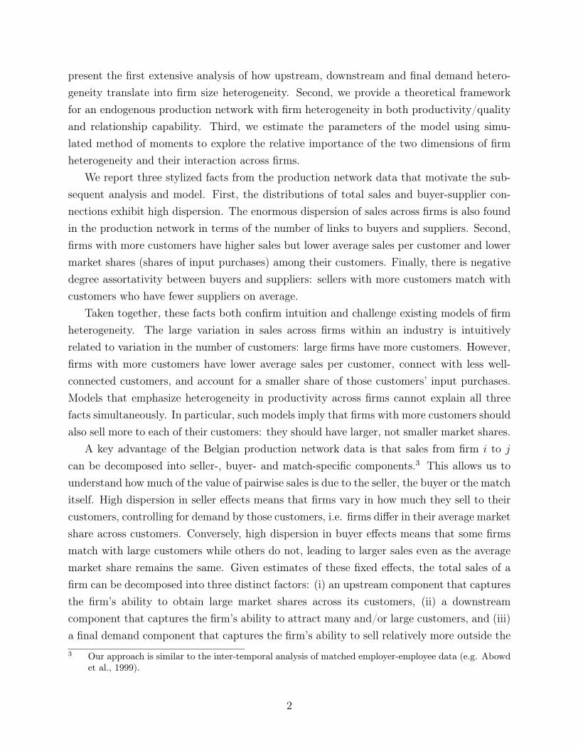
Fact 1. The distributions of firm sales and supplier-buyer connections are highly dispersed.

Even within narrowly defined industries, firms show significant heterogeneity along sev-eral dimensions.8 Figure 1 documents the distributions of firm size and the number ofcustomers and suppliers for Belgian firms. All variables are demeaned at the 4-digit NACEindustry.9 Panel (a) shows the firm size distribution, expressed in total sales value. As iswell-known, the distribution spans several orders of magnitude: relative to the average firmin its industry, some firms are up to four orders of magnitude larger, and they co-exist withvery small firms several orders of magnitude smaller than the average. Panel (b) reports thedistribution of the number of customers of these firms. Here as well, firms can have over1,000 times as many customers as their industry average, again co-existing with firms thathave few customers. Similarly, in panel (c), the number of suppliers is shown. While less8 These patterns mirror findings for firm-to-firm linkages in the domestic production network in Belgium

(Dhyne et al., 2015) and Japan (Bernard et al., 2019) and for firm-to-firm export transactions in Norway(Bernard et al., 2018a).

9 We demean variables by regressing log variables on 4-digit sector fixed effects and retain the residualsas demeaned log variables.

7

(a)

(b) (c)

Figure 1: Distribution of firm sales, number of customers and number of suppliers.

excessive, again this distribution spans several orders of magnitude. Appendix B reportsadditional moments on both demeaned and raw variables.

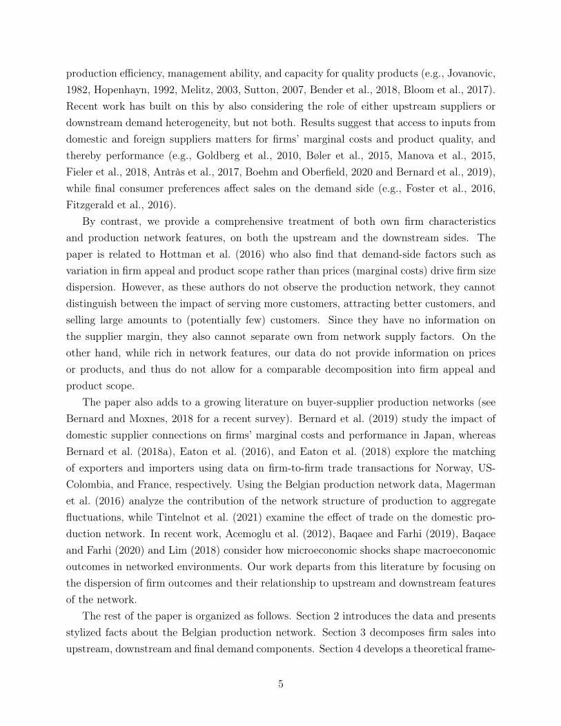
Fact 2. Firms with more customers have higher sales but lower sales per customer.

A sharp pattern in the data is that firms with more customers have higher sales but lowersales per customer. Figure 2a displays the binned scatterplot of firm sales to other producersin the network (y-axis) against the number of customers (x-axis), on a log-log scale. Bothvariables are demeaned by their 4-digit industry average, and observations are binned into20 quantiles. The elasticity of sales with respect to the number of buyers is 0.77. Therefore,sales increases in the number of customers, but less than proportionally. This directly implies

8

that sales per customer decreases with the number of customers, as illustrated in Figure 2b,with an elasticity of −0.23.10

This pattern is not driven by composition effects among customers. Figure 3a demon-strates that sales per customer fall with the number of customers for both big and smallcustomers. For each firm, we calculate the 10th, 50th and 90th percentiles of sales across itsbuyers, and plot these percentiles against the firm’s number of buyers. The slope coefficientsare negative, and range between -.13 and -.22. This implies that firms do not systematicallytend to sell relatively more or less to their top customers at the expense of their bottomcustomers, when they add more buyers.

One may also wonder if the decline in average sales per customer is driven by selection.If sellers match with smaller buyers when they grow their customer base, they would recordlower average and median bilateral sales. To address this concern, we leverage the networkdata and calculate a firm’s weighted average market share among its customers: the geo-metric mean of mij/M

netj , where mij is sales from i to j and Mnet

j is total network purchasesby firm j, using sales shares mij/S

neti as weights.11 If selection were the main mechanism,

this weighted average market share would be increasing in, or unrelated to, the number ofcustomers. Figure 3b shows that this is not the case: Firms’ weighted average market sharealso declines with their number of customers, with an elasticity of -0.08.

We explore the potential impact of additional dimensions of customer heterogeneity inAppendix B. In particular, we control for heterogeneity in input requirements across cus-tomers within the seller’s industry. We also consider the role of fringe buyers, i.e. relativelyunimportant customers in terms of mij. In all cases, our empirical findings retain the samemessage. Taken together, these empirical regularities present a puzzle: big firms match withmany buyers, but they are unable to gain a large market share among those buyers. Bycontrast, in canonical one-dimensional models of firm heterogeneity, or models with two ormore, but independent, dimensions (e.g., Arkolakis, 2010, Bernard et al., 2018a, Eaton etal., 2018, Lim, 2018), highly productive firms would both attract many customers and havea high market share among those customers. The empirical evidence therefore calls for amodel with an additional element of firm heterogeneity, where firm size is not only deter-10 We construct total domestic network sales as Sneti =

∑jmij . We thus obtain an identity between Sneti ,

the number of customers nci and the average sales per customer, as Sneti

nci

= 1nci

∑jmij . Note that this

identity implies that the elasticities in Figures 2a and 2b amount to 0.77− (−.23) = 1. As we observetotal sales Si, but not the number of customers in export destinations, this identity would no longerhold if using Si instead of Sneti . However, all results are very similar and qualitatively the same whenusing total sales instead of network sales.

11 I.e., the weighted average market share is δi =∏j

(mij

Mnetj

) mij

Sneti . The weighted average puts less emphasis

on fringe customers. Using the unweighted average however, produces similar results.

9

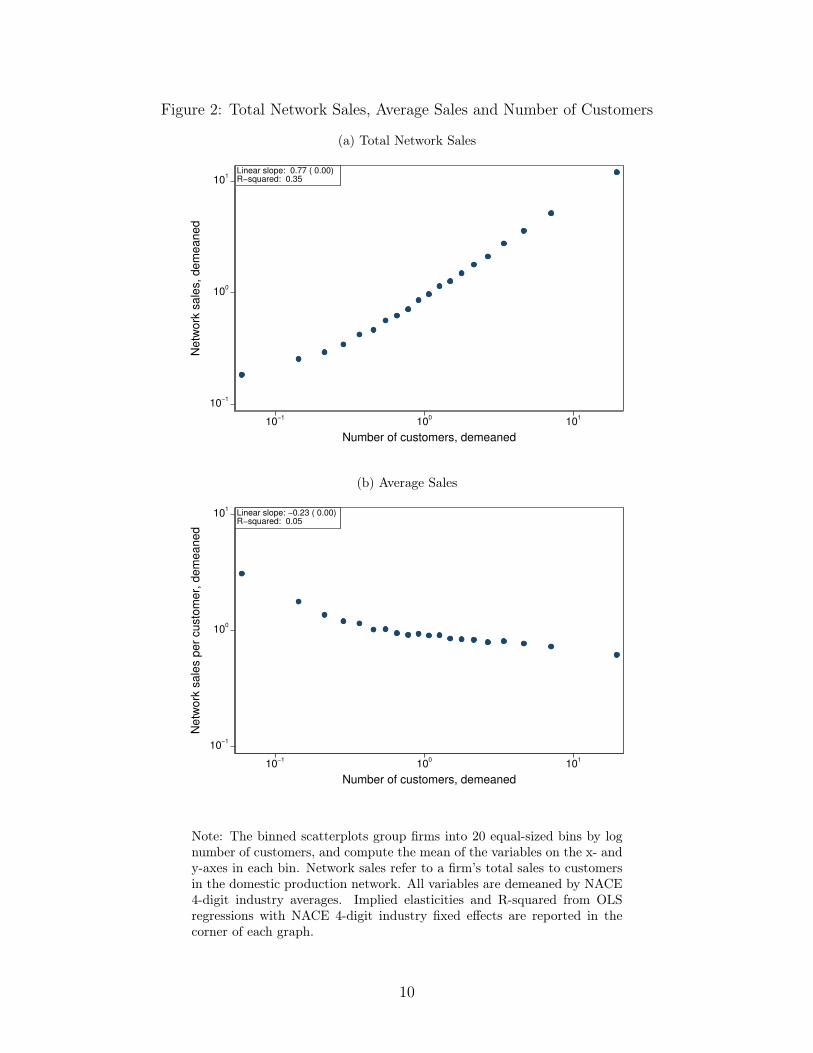
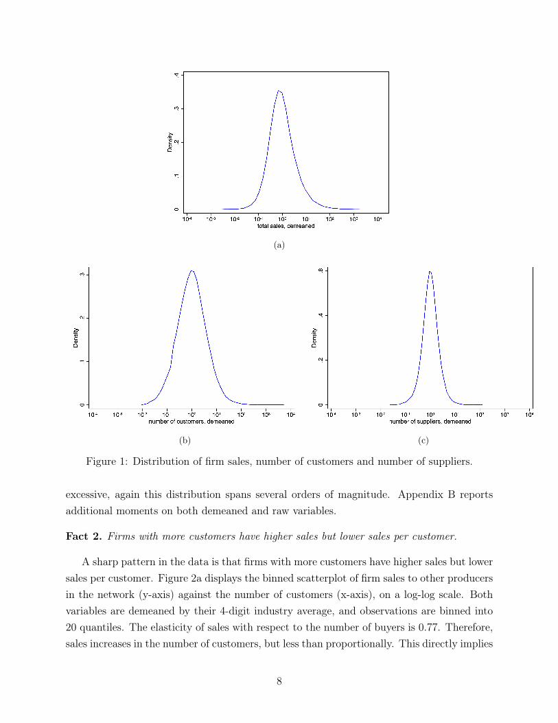
Figure 2: Total Network Sales, Average Sales and Number of Customers

(a) Total Network Sales

10−1

100

101

Netw

ork

sale

s, dem

eaned

10−1

100

101

Number of customers, demeaned

Linear slope: 0.77 ( 0.00)R−squared: 0.35

(b) Average Sales

10−1

100

101

Netw

ork

sale

s p

er

custo

mer,

dem

eaned

10−1

100

101

Number of customers, demeaned

Linear slope: −0.23 ( 0.00)R−squared: 0.05

Note: The binned scatterplots group firms into 20 equal-sized bins by lognumber of customers, and compute the mean of the variables on the x- andy-axes in each bin. Network sales refer to a firm’s total sales to customersin the domestic production network. All variables are demeaned by NACE4-digit industry averages. Implied elasticities and R-squared from OLSregressions with NACE 4-digit industry fixed effects are reported in thecorner of each graph.

10

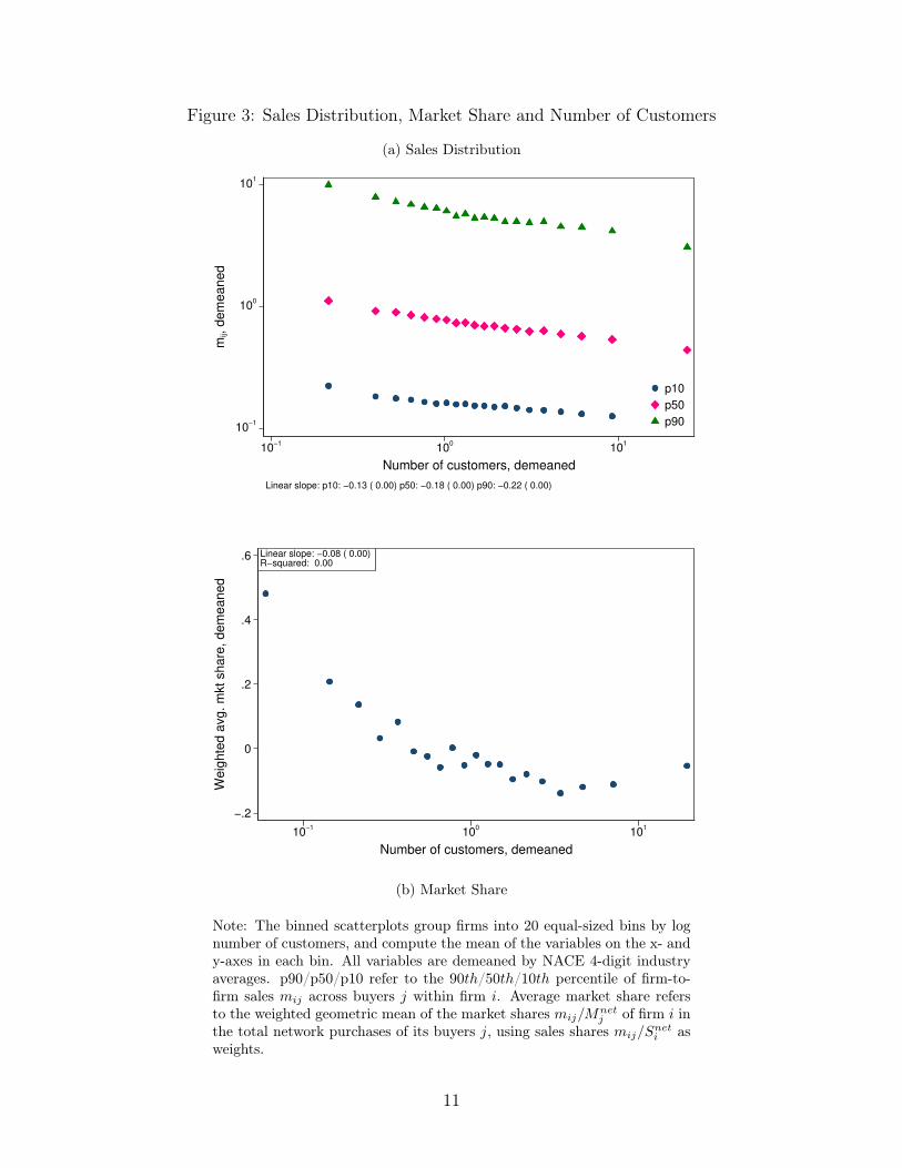
Figure 3: Sales Distribution, Market Share and Number of Customers

(a) Sales Distribution

10−1

100

101

mij, d

em

eaned

10−1

100

101

Number of customers, demeaned

p10

p50

p90

Linear slope: p10: −0.13 ( 0.00) p50: −0.18 ( 0.00) p90: −0.22 ( 0.00)

−.2

0

.2

.4

.6

Weig

hte

d a

vg. m

kt share

, dem

eaned

10−1

100

101

Number of customers, demeaned

Linear slope: −0.08 ( 0.00)R−squared: 0.00

(b) Market Share

Note: The binned scatterplots group firms into 20 equal-sized bins by lognumber of customers, and compute the mean of the variables on the x- andy-axes in each bin. All variables are demeaned by NACE 4-digit industryaverages. p90/p50/p10 refer to the 90th/50th/10th percentile of firm-to-firm sales mij across buyers j within firm i. Average market share refersto the weighted geometric mean of the market shares mij/M

netj of firm i in

the total network purchases of its buyers j, using sales shares mij/Sneti as

weights.

11

mined by productivity, but also by a second firm attribute that enables firms to match withmore buyers.

Fact 3. Sellers with more customers match with customers who have fewer suppliers onaverage.

An important property of networks is the extent to which a well-connected node is linkedto other well-connected nodes, so-called degree assortativity. The production network ischaracterized by negative degree assortativity. In other words, better connected firms matchto less well-connected firms on average.12 Figure 4 shows a binned scatterplot of the averagenumber of suppliers to firm i’s customers on the y-axis against the number of i’s customers,on a log-log scale. The fitted regression line has slope -0.05, such that doubling the numberof customers is associated with a 5 percent decline in the average customer’s number ofsuppliers. We also find a robust, and more negative, relationship between a firm’s numberof suppliers and the average supplier’s number of customers (see Table 5 in Section 5.2).

Negative degree assortativity motivates our choice of a parsimonious matching model, inwhich firm connections form whenever the gross profits of a match exceed the fixed cost offorming a relationship. In this class of models, the marginal (and average) customer of morecapable firms is less capable, generating a pattern of negative degree assortativity.

3 An Exact Decomposition

In this section, we develop an exact variance decomposition of firm sales into upstream,downstream, and final demand margins. The downstream component reflects characteristicsof a firm’s customers (i.e., their number and size), while the upstream component capturesfirm characteristics that remain constant across customers (i.e., average sales to customers,controlling for their size). Final demand includes factors unrelated to the domestic produc-tion network (i.e., sales to final consumers or foreign customers). This method exploits thegranularity of the firm-to-firm transaction data in a way that would not be feasible with stan-dard firm-level datasets, and its results provide the rationale for the structural framework inSection 4.

3.1 Methodology

We start by estimating buyer, seller and buyer-seller match effects using data on sales betweenfirms in the production network. We then use these estimates to decompose the variance of12 Negative degree assortativity has been documented in earlier research on production networks, e.g.

Bernard et al. (2019), Bernard et al. (2018a) and Lim (2018).

12

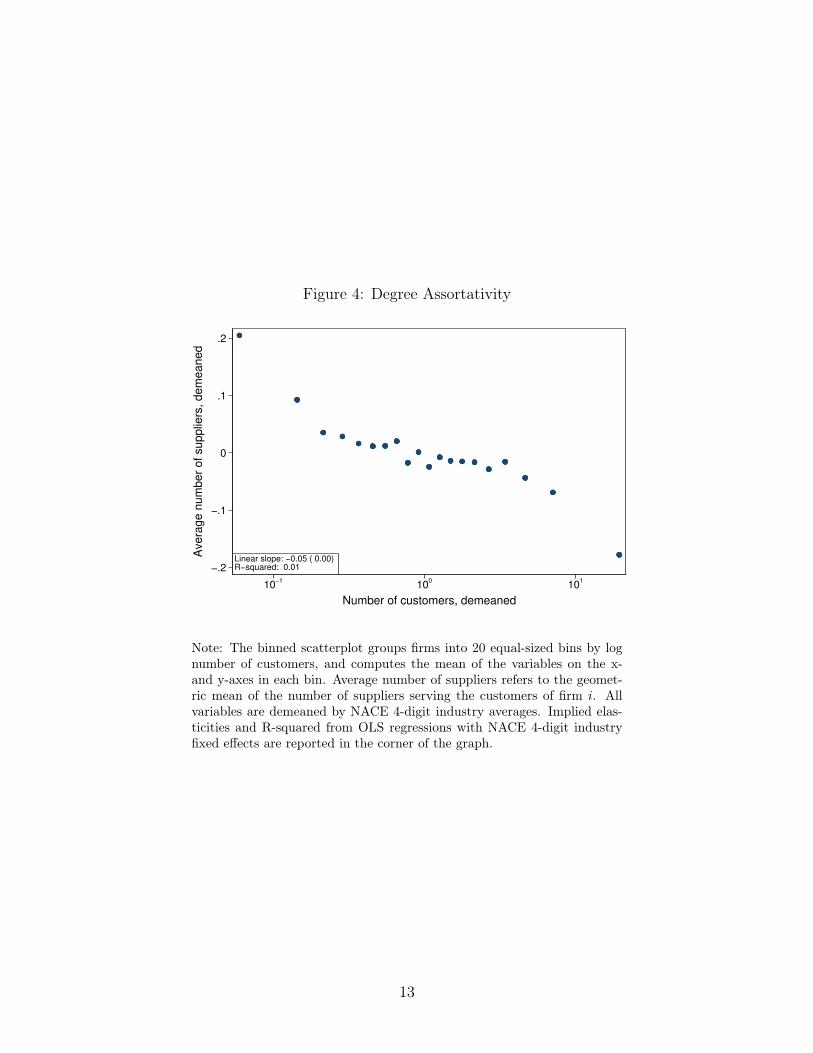
Figure 4: Degree Assortativity

−.2

−.1

0

.1

.2

Avera

ge n

um

ber

of supplie

rs, dem

eaned

10−1

100

101

Number of customers, demeaned

Linear slope: −0.05 ( 0.00)R−squared: 0.01

Note: The binned scatterplot groups firms into 20 equal-sized bins by lognumber of customers, and computes the mean of the variables on the x-and y-axes in each bin. Average number of suppliers refers to the geomet-ric mean of the number of suppliers serving the customers of firm i. Allvariables are demeaned by NACE 4-digit industry averages. Implied elas-ticities and R-squared from OLS regressions with NACE 4-digit industryfixed effects are reported in the corner of the graph.

13

firm sales. The specification is a two-way fixed effects regression for firm-to-firm sales:

lnmij = lnG+ lnψi + ln θj + lnωij, (1)

where lnmij is log sales from i to j, and lnG is the mean of lnmij across all ij pairs. Theseller effect lnψi reflects the amount of sales by i to its average customer j, controllingfor total purchases by j via θj. The seller effect is therefore related to the average marketshare of i among her customers.13 Analogously, the buyer effect ln θj captures the valueof input purchases by j from its average supplier i, controlling for total sales by i via ψi.Intuitively, attractive buyers (high θj) purchase a disproportionate share of suppliers’ sales.Finally, lnωij is the residual from the regression. A positive lnωij reflects match-specificcharacteristics that induce a given firm pair to trade more with each other, even if they arenot fundamentally attractive trade partners.

To illustrate the advantage of the bilateral sales data, consider first an extreme casein which the variation in lnmij is only due to ψi. Seller i is then larger than seller i′

because i sells more to every customer, while there is no variation in how much each ofthese customers buys from i. In this case, firm size heterogeneity is only driven by sellercharacteristics ψi; who you are as a seller explains firm size. Consider next the oppositecase in which the variance in lnmij is only due to θj. Seller i now dominates seller i′

because i matches with bigger customers than i′, while sales to common customers j areidentical. In this case, firm heterogeneity is only driven by differences in matching abilityacross sellers; who you meet as a seller explains firm size. In standard firm-level datasets, wecannot differentiate between these two scenarios because they are observationally equivalent.Estimating equation (1) using OLS poses some threats to identification. First, to obtainunbiased estimates, the assignment of suppliers to customers must be exogenous with respectto ωij, so-called conditional exogenous mobility (Abowd et al., 1999). This assumption, aswell as tests for exogenous mobility and functional form relevance, are discussed at lengthin Appendix C. Overall, we find strong support for the log-linear model and the conditionalexogenous mobility assumption.

Second, to identify the fixed effects, firms must have multiple connections. Specifically,identifying a seller fixed effect requires a firm to have at least two customers, and identifyinga buyer fixed effect requires a firm to have at least two suppliers. Therefore, single-customerand single-supplier links are dropped in the estimation procedure. Also, dropping customerA might result in supplier B having only one customer left. Supplier B is then also removedfrom the sample. This iterative process continues until a connected network component13 This is shown formally in Appendix D.2.

14

remains (i.e. a within-projection matrix of full rank), in which each seller has at least twocustomers and each buyer has at least two suppliers. This component is known as a mobilitygroup in the labor literature on firm-employee matches.

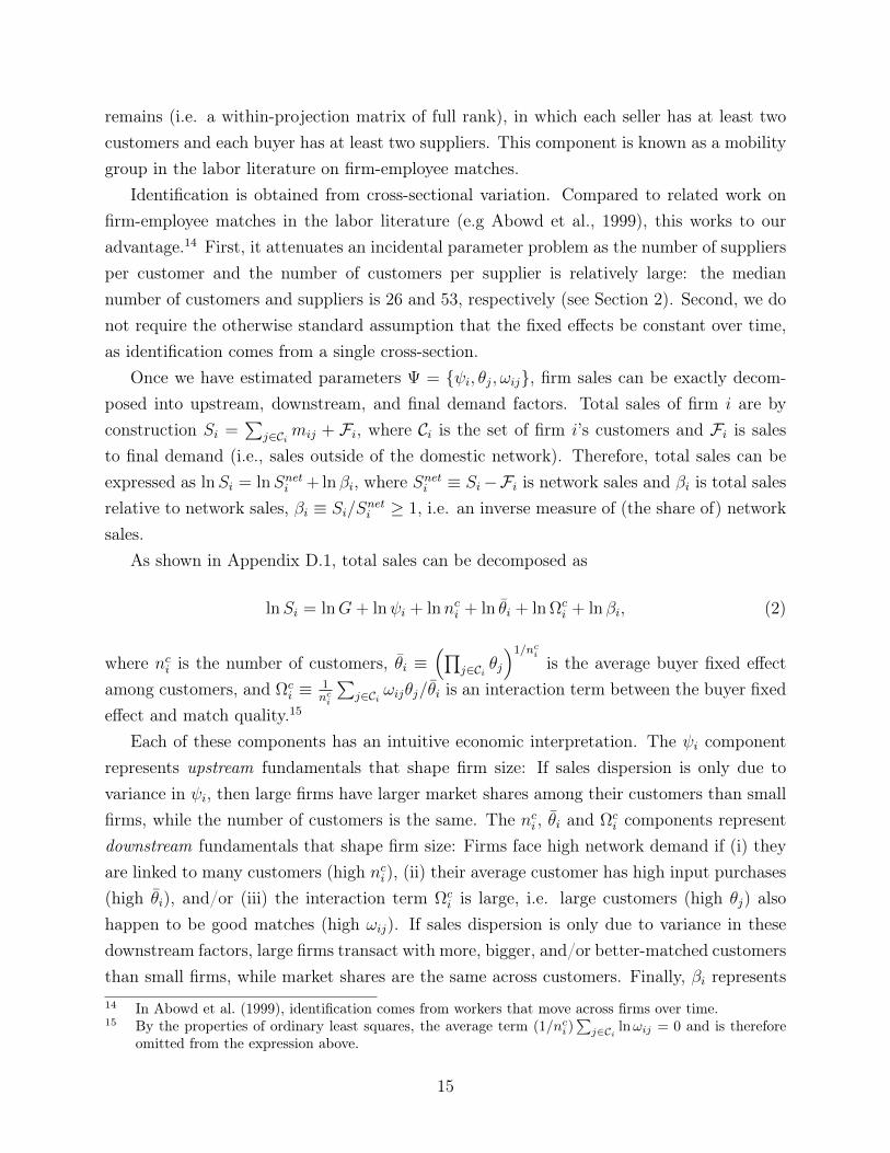
Identification is obtained from cross-sectional variation. Compared to related work onfirm-employee matches in the labor literature (e.g Abowd et al., 1999), this works to ouradvantage.14 First, it attenuates an incidental parameter problem as the number of suppliersper customer and the number of customers per supplier is relatively large: the mediannumber of customers and suppliers is 26 and 53, respectively (see Section 2). Second, we donot require the otherwise standard assumption that the fixed effects be constant over time,as identification comes from a single cross-section.

Once we have estimated parameters Ψ = ψi, θj, ωij, firm sales can be exactly decom-posed into upstream, downstream, and final demand factors. Total sales of firm i are byconstruction Si =

∑j∈Ci mij + Fi, where Ci is the set of firm i’s customers and Fi is sales

to final demand (i.e., sales outside of the domestic network). Therefore, total sales can beexpressed as lnSi = lnSneti + ln βi, where Sneti ≡ Si−Fi is network sales and βi is total salesrelative to network sales, βi ≡ Si/S

neti ≥ 1, i.e. an inverse measure of (the share of) network

sales.As shown in Appendix D.1, total sales can be decomposed as

lnSi = lnG+ lnψi + lnnci + ln θi + ln Ωci + ln βi, (2)

where nci is the number of customers, θi ≡(∏

j∈Ci θj

)1/nci

is the average buyer fixed effectamong customers, and Ωc

i ≡ 1nci

∑j∈Ci ωijθj/θi is an interaction term between the buyer fixed

effect and match quality.15

Each of these components has an intuitive economic interpretation. The ψi componentrepresents upstream fundamentals that shape firm size: If sales dispersion is only due tovariance in ψi, then large firms have larger market shares among their customers than smallfirms, while the number of customers is the same. The nci , θi and Ωc

i components representdownstream fundamentals that shape firm size: Firms face high network demand if (i) theyare linked to many customers (high nci), (ii) their average customer has high input purchases(high θi), and/or (iii) the interaction term Ωc

i is large, i.e. large customers (high θj) alsohappen to be good matches (high ωij). If sales dispersion is only due to variance in thesedownstream factors, large firms transact with more, bigger, and/or better-matched customersthan small firms, while market shares are the same across customers. Finally, βi represents14 In Abowd et al. (1999), identification comes from workers that move across firms over time.15 By the properties of ordinary least squares, the average term (1/nci )

∑j∈Ci lnωij = 0 and is therefore

omitted from the expression above.

15

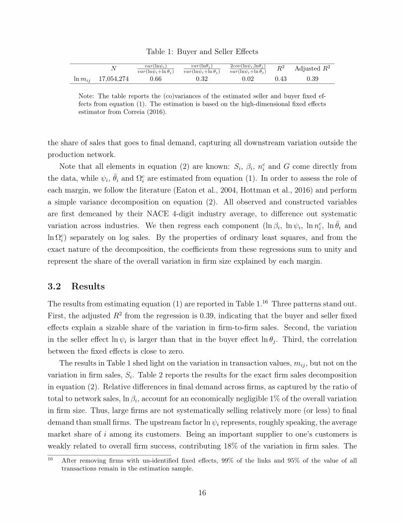
Table 1: Buyer and Seller Effects

N var(lnψi)var(lnψi+ln θj)

var(lnθj)var(lnψi+ln θj)

2cov(lnψi,lnθj)var(lnψi+ln θj) R2 Adjusted R2

lnmij 17,054,274 0.66 0.32 0.02 0.43 0.39

Note: The table reports the (co)variances of the estimated seller and buyer fixed ef-fects from equation (1). The estimation is based on the high-dimensional fixed effectsestimator from Correia (2016).

the share of sales that goes to final demand, capturing all downstream variation outside theproduction network.

Note that all elements in equation (2) are known: Si, βi, nci and G come directly fromthe data, while ψi, θi and Ωc

i are estimated from equation (1). In order to assess the role ofeach margin, we follow the literature (Eaton et al., 2004, Hottman et al., 2016) and performa simple variance decomposition on equation (2). All observed and constructed variablesare first demeaned by their NACE 4-digit industry average, to difference out systematicvariation across industries. We then regress each component (ln βi, lnψi, lnnci , ln θi andln Ωc

i) separately on log sales. By the properties of ordinary least squares, and from theexact nature of the decomposition, the coefficients from these regressions sum to unity andrepresent the share of the overall variation in firm size explained by each margin.

3.2 Results

The results from estimating equation (1) are reported in Table 1.16 Three patterns stand out.First, the adjusted R2 from the regression is 0.39, indicating that the buyer and seller fixedeffects explain a sizable share of the variation in firm-to-firm sales. Second, the variationin the seller effect lnψi is larger than that in the buyer effect ln θj. Third, the correlationbetween the fixed effects is close to zero.

The results in Table 1 shed light on the variation in transaction values,mij, but not on thevariation in firm sales, Si. Table 2 reports the results for the exact firm sales decompositionin equation (2). Relative differences in final demand across firms, as captured by the ratio oftotal to network sales, ln βi, account for an economically negligible 1% of the overall variationin firm size. Thus, large firms are not systematically selling relatively more (or less) to finaldemand than small firms. The upstream factor lnψi represents, roughly speaking, the averagemarket share of i among its customers. Being an important supplier to one’s customers isweakly related to overall firm success, contributing 18% of the variation in firm sales. The16 After removing firms with un-identified fixed effects, 99% of the links and 95% of the value of all

transactions remain in the estimation sample.

16

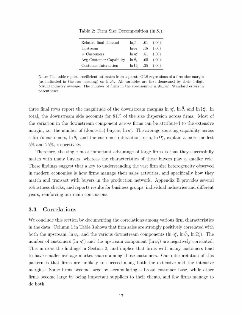
Table 2: Firm Size Decomposition (lnSi).

Relative final demand lnβi .01 (.00)Upstream lnψi .18 (.00)# Customers lnnci .51 (.00)Avg Customer Capability ln θi .05 (.00)Customer Interaction ln Ωci .25 (.00)

Note: The table reports coefficient estimates from separate OLS regressions of a firm size margin(as indicated in the row heading) on lnSi. All variables are first demeaned by their 4-digitNACE industry average. The number of firms in the core sample is 94,147. Standard errors inparentheses.

three final rows report the magnitude of the downstream margins lnnci , ln θi and ln Ωci . In

total, the downstream side accounts for 81% of the size dispersion across firms. Most ofthe variation in the downstream component across firms can be attributed to the extensivemargin, i.e. the number of (domestic) buyers, lnnci . The average sourcing capability acrossa firm’s customers, ln θi, and the customer interaction term, ln Ωc

i , explain a more modest5% and 25%, respectively.

Therefore, the single most important advantage of large firms is that they successfullymatch with many buyers, whereas the characteristics of these buyers play a smaller role.These findings suggest that a key to understanding the vast firm size heterogeneity observedin modern economies is how firms manage their sales activities, and specifically how theymatch and transact with buyers in the production network. Appendix E provides severalrobustness checks, and reports results for business groups, individual industries and differentyears, reinforcing our main conclusions.

3.3 Correlations

We conclude this section by documenting the correlations among various firm characteristicsin the data. Column 1 in Table 3 shows that firm sales are strongly positively correlated withboth the upstream, lnψi, and the various downstream components (lnnci , ln θi, ln Ωc

i). Thenumber of customers (ln nci) and the upstream component (lnψi) are negatively correlated.This mirrors the findings in Section 2, and implies that firms with many customers tendto have smaller average market shares among those customers. Our interpretation of thispattern is that firms are unlikely to succeed along both the extensive and the intensivemargins: Some firms become large by accumulating a broad customer base, while otherfirms become large by being important suppliers to their clients, and few firms manage todo both.

17

Table 3: Correlation Matrix

Firm Size Component lnSi lnψi lnnci ln θi ln Ωci lnβi

lnSi 1lnψi 0.23 1lnnci 0.49 -0.33 1ln θi 0.20 0.22 -0.18 1ln Ωci 0.45 0.16 0.09 0.23 1lnβi 0.02 -0.36 -0.33 -0.16 -0.42 1

Note: All correlations are significant at 5%. All variables are demeaned atthe NACE 4-digit level.

These results, coupled with the stylized facts and sales decomposition, are difficult toreconcile with canonical heterogenous-firm models. They suggest that both upstream anddownstream dimensions of firm activity underpin sales dispersion when firms interact inproduction networks. One interpretation of our findings is that firm attributes that matterfor matching with customers and suppliers are orthogonal, or even negatively related, to firmattributes that determine sales conditional on a match.

4 Theoretical Framework

Motivated by the stylized facts, this section develops a theoretical framework of a buyer-supplier production network with two-sided firm heterogeneity and endogenous match forma-tion. This framework admits a two-step analysis: We first present the model conditional ona set of firm-to-firm links, and subsequently introduce a parsimonious firm-to-firm matchingmodel.

Our starting point is a framework in which firms are heterogeneous in two dimensions.First, firms within an industry have different productivities, which implies that they havedifferent marginal costs and prices.17 Second, firms have different relationship capabili-ties. These capabilities determine their ability to match with customers conditional on their(quality-adjusted) prices. We model relationship capability as a fixed cost that the firm mustincur for each customer it chooses to serve. A firm with lower relationship fixed costs willendogenously be able to match with more customers, all else equal. In contrast to much ofthe earlier literature, productivity and relationship capability are potentially correlated.17 As is standard in this class of models, under the assumption of CES preferences and monopolistic

competition, productivity and product quality enter equilibrium firm revenue in exactly the same way.

18

Firms operate in a production network, sourcing their inputs from other firms and sellingtheir output to both other firms and final demand. In addition to productivity and relation-ship capability, a firm’s size thus also depends on its input prices. Input prices are low andsales high if the firm has many low-price (or high-quality) suppliers.

4.1 Technology and Demand

The economy consists of a unit continuum of firms, each with the following productionfunction:

y (i) = κz (i) l (i)α v (i)1−α ,

where y (i) is output (in quantities) of firm i, z (i) is productivity, l (i) is the amount oflabor used by firm i, α is the labor share, and κ > 0 is a normalization constant.18 v (i) is aconstant-elasticity-of-substitution (CES) input bundle:

v (i) =

(∫S(i)

ν (k, i)(σ−1)/σ dk

)σ/(σ−1)

,

where ν (k, i) is the quantity purchased from firm k, S (i) is the set of suppliers to firm i, andσ > 1 is the elasticity of substitution across suppliers. The corresponding input price index

is P (i) =(∫S(i)

p (k)1−σ dk)1/(1−σ)

, where p (k) is the price charged by supplier k. Settingthe wage w as the numéraire, the marginal cost of the firm is:

c (i) =P (i)1−α

z (i). (3)

Final Demand. Final consumers have a CES utility function with the same elasticity ofsubstitution σ across output varieties. The representative consumer is the shareholder of allfirms, so that aggregate profits Π become part of consumer income. Aggregate income X istherefore the sum of aggregate labor income and aggregate corporate profits, X = wL+ Π,where L is inelastically supplied labor.

18 κ ≡ α−α (1− α)−(1−α). This normalization maps the production function to the cost function, and

simplifies the expression for the cost function, without any bearing on our results.

19

4.2 Firm-to-Firm Sales

Each firm faces demand from other firms, as well as from final consumers. Given the as-sumptions about technology, sales from firm i to firm j are:

m (i, j) = p (i)1−σ P (j)σ−1M (j) , (4)

where M (j) are total intermediate purchases by firm j, M (j) =∫S(j)

m (i, j) di.The market structure is monopolistic competition, such that firms charge a constant

mark-up over marginal costs, p (i) = µc (i), where µ ≡ σ/ (σ − 1). After rearranging, salesfrom i to j can be expressed as:

m (i, j) =

[z (i)

µP (i)1−αP (j)

]σ−1

M (j) . (5)

The model thus delivers a simple log linear expression for firm-to-firm sales, just as in thereduced-form equation (1) in Section 3.

4.3 Equilibrium Conditional on Network

We characterize the equilibrium in two separable steps. This section first describes proper-ties of the partial equilibrium conditional on a fixed network structure. The next sectionthen develops the firm-to-firm matching model, and specifies the general equilibrium withendogenous match formation.

To proceed, we introduce additional notation. A firm i is characterized by the tupleλ = (z, F ), where z is productivity and F is a relationship fixed cost, in units of labor. zand F are potentially correlated, and dG (λ) denotes the (multivariate) density of λ. Wedefine the link function l (λ, λ′) as the share of seller-buyer pairs (λ, λ′) that match.19

Backward fixed point. For a given network structure, the equilibrium can be found bysolving for two fixed points sequentially. Using the pricing rule p (λ) = µc (λ) and theequation for marginal costs (3), the input price index can be solved by iterating on a backwardfixed point problem:

P (λ)1−σ = µ1−σ∫P (λ′)

(1−σ)(1−α)z (λ′)

σ−1l (λ′, λ) dG (λ′) . (6)

19 Due to idiosyncratic pairwise fixed cost shocks, the link function will take values between 0 and 1, seeSection 4.4.

20

The input cost index of firm λ, P (λ), depends on the input cost index and productivity ofall its suppliers λ′, P (λ′) and z (λ′).

Forward fixed point. Sales of a type-λ firm are the sum of sales to final and intermediatedemand: S (λ) = F (λ) +

∫m (λ, λ′) l (λ, λ′) dG (λ′), where m (λ, λ′) now denotes sales by

supplier λ to buyer λ′. Final demand is F (λ) = p (λ)1−σ Pσ−1X, with the consumer priceindex equal to P1−σ =

∫p (λ)1−σ dG (λ) = µ1−σ ∫ P (λ)(1−σ)(1−α) z (λ)σ−1 dG (λ). Also note

that total input purchases are M (λ) = S (λ) (1− α) /µ. Using this together with equation(3) yields:

S (λ) = µ1−σz (λ)σ−1 P (λ)(1−σ)(1−α)

(X

P1−σ +1− αµ

∫S (λ′)

P (λ′)1−σ l (λ, λ′) dG (λ′)

). (7)

Sales of a type-λ firm depend on final demand, X, the productivity and input price indexof the firm itself, z (λ) and P (λ), and the sales and input prices of its customers, S (λ′) andP (λ′). Appendix D.3 proves the existence and uniqueness of the equilibrium.

4.4 Firm-to-Firm Matching

We now consider the general equilibrium when the production network is endogenous andsellers match with buyers if and only if the profits from doing so are positive. The sellerincurs a relationship fixed cost Fε for every buyer it chooses to sell to, where F varies acrosssellers, and ε is an idiosyncratic component that varies across firm pairs. This matchingmodel is similar to Bernard et al. (2018a) and Lim (2018), but in contrast to these papers,F is a firm-specific attribute that can be correlated with the productivity of the firm, z.20

The share of seller-buyer pairs (λ, λ′) that match and trade with each other is then:

l (λ, λ′) =

∫I [ln ε < ln π (λ, λ′)− lnF ] dH (ε) , (8)

where I[] is the indicator function, dH (ε) denotes the density of ε, and the gross profits fromthe potential match are:

π (λ, λ′) =m (λ, λ′)

σ.

The introduction of idiosyncratic match costs ε is not needed to solve the model or torationalize the stylized facts presented earlier in the paper. However, ε will play a role in thestructural estimation in Section 5. Formally, dispersion in ε ensures that the link functionis continuous in the parameters of the model, such that standard gradient-based numerical20 On the other hand, sales to final demand incur no fixed costs and vary across firms only due to differences

in output prices.

21

methods can be used to minimize the objective function. Intuitively, ε can be justified withseller-buyer specific costs that affect the profitability of the relationship, such as the fixedcost of adapting the seller’s output to the buyer’s production needs.

This link function is also a fixed point problem. The gross profits from a potentialmatch, π(), determine link probabilities according to equation (8), and the link probabilitiesdetermine gross profits via the backward and forward fixed points in equations (6) and (7).

The general equilibrium of the model can be solved by a simple nested fixed point algo-rithm. (i) Start with a guess for the link function l(). (ii) Solve for P (λ) and S (λ) using thebackward and forward fixed points in equations (6) and (7) sequentially. (iii) Calculate grossprofits for all potential matches using equation (5). (iv) Calculate the share of seller-buyerpairs (λ, λ′) that match according to equation (8). (v) Go back to step (ii) until the linkfunction converges. We do not have a formal proof of existence and uniqueness. In practice,however, the nested fixed point problem is numerically well-behaved and always convergesto the same solution irrespective of the chosen starting values.

4.5 Discussion

We conclude the exposition of the model by discussing some key implications and features.We start by considering the role of each dimension of firm heterogeneity in determiningequilibrium outcomes on its own. Conditioning on relationship capability, firms with higherproductivity have lower marginal costs, lower prices and higher profits from a match withany given buyer, see equation (3). As a result, higher productivity firms match with morebuyers, see equation (8), and have greater sales (market share) conditional on a match, seeequation (5). Larger total sales and input purchases make higher productivity firms moreattractive partners for upstream firms, see equation (5). The increased number of upstreamsuppliers contributes to an additional reduction in marginal cost through the firm’s inputprice index, see equation (6).

Conditioning on productivity, firms with better relationship capability, lower F , are ableto match with more buyers, see equation (8), and as a result have greater sales and greaterinput purchases. As with higher productivity, the greater input demand makes these firmsrelatively attractive to upstream suppliers, and the greater number of suppliers lowers theirmarginal cost of production through the input price index. The lower marginal cost resultsin greater sales (market share) to any given buyer.

Thus considered by itself, either higher productivity or better relationship capabilityleads to higher sales through both the extensive margin of more downstream buyers and theintensive margin of greater sales per buyer.

22

Several features of the model grant it analytical and quantitative tractability, as well astransparency in illustrating the main mechanisms. First, we consider a unit continuum offirms in the economy. This implies that individual sellers take other sellers’ prices and allbuyers’ input price indices as given when deciding whether to match with a particular buyerand how much to sell to that buyer.

Separately, we focus on the costs that sellers incur to match with buyers, and assumethat buyers do not face corresponding costs of matching with suppliers. Even with thisassumption, in equilibrium the number of both suppliers and buyers varies across firms.This choice lends tractability because firms make separable sales decisions with respect todifferent buyers and do not internalize the effect of their match decisions on buyers’ inputdemand. It also avoids the well-known problem of interdependence of sourcing decisions inframeworks where buyers choose suppliers, see Antràs et al. (2017).

Finally, the model focuses on the domestic production network and does not directlyconsider the role of exports and imports, both of which are important in the Belgian context.Exports are implicitly included in final demand, even though this almost surely understatesthe importance of firm-to-firm sales, as almost all export sales are to firms rather thanconsumers. Similarly, while we do not model imports, they can be added to productionwithout changing the implications for firm outcomes.21

5 Estimation and Results

This section provides a model-based assessment of the origins of firm heterogeneity. Specif-ically, we exploit the Belgian production network data to parameterize the model above,allowing for heterogeneity in both productivity and relationship capability across firms. Wethen estimate the model under alternative scenarios to evaluate the quantitative importanceof each firm attribute.

5.1 Simulated Method of Moments

The general-equilibrium model is estimated by simulated method of moments (SMM). Weassume that firm productivity z and relationship capability F are distributed joint log-normal with expectations µln z = 0 and µlnF , standard deviations σln z and σlnF , andcorrelation coefficient ρ.22 In sum, there are four unknown parameters to be estimated,21 See Bernard et al. (2018b) for a static model of a domestic production network with imports in the

production function and idiosyncratic match-specific shocks.22 The mean of ln z is not identified, and it is therefore normalized to zero. This normalization is appealing

on conceptual grounds. Consider a shift in the productivity distribution, such that productivity increases

23

Υ = σln z, µlnF , σlnF , ρ.In addition to the unknown parameters, information is needed on α (labor cost share),

µ (markup), and X (aggregate income). α is constructed by dividing labor costs by totalcosts for each firm, and then taking the simple average across firms. µ is computed bydividing sales by total costs for each firm, and then taking the simple average across firms.X is inferred from sales going out of the network, i.e. X =

∑i Si −

∑i

∑j∈Ci mij. The

idiosyncratic matching cost ε is assumed log-normal, with mean µln ε = 0 and standarddeviation σln ε. The standard deviation is chosen so that the objective function is smoothin the parameters of the model.23 Table 4 summarizes the parameters of the model, theirdefinitions, and the values assigned to them.

We choose seven moments in the data to estimate Υ. While all moments jointly pin downall unknown parameters in general equilibrium, there is an intuitive mapping between them.First, the mean log number of customers across firms,mean (lnnci), helps identify the mean ofthe relationship costs. Second, the variance of log number of customers, var (lnnci), and thevariance of network sales, var (lnSneti ), together identify the variances of productivity andrelationship costs. Third, the slope coefficient from the regression of average market shareon the number of buyers, ln δi = α + β lnnci + εi, helps identify the correlation coefficient ρ(see Figure 3): implicitly, a smaller (or more negative) slope coefficient suggests that firmswith low relationship costs and therefore high lnnci are relatively less productive and thushave lower ln δi. Finally, we include the contribution of key decomposition margins in Table2: the number of customers (lnnci), average customer capability (ln θi), and the customerinteraction term (ln Ωc

i). Intuitively, the contribution of these margins to firm size dispersioninform the role of relationship costs versus productivity in determining firm size.24 Collectingthe targeted empirical moments in vector x and the corresponding simulated moments invector xs (Υ), the SMM estimates for Υ solve:

arg minΥ

(x− xs (Υ))′ (x− xs (Υ)) .

We obtain standard errors by bootstrapping these estimates, see Appendix F for details.25

for all firms. While this would lower prices and increase welfare, it would not change firms’ market sharesor the network structure of the economy that are of interest to us.

23 If the dispersion in ε is small relative to the dispersion in z and F , the share of links for some (λ, λ′) pairswill be close to zero. This complicates the SMM estimation using standard gradient-based methods, asthe objective function is no longer smooth in the parameters of the model. In practice, we set σln ε = 4,which makes the problem sufficiently smooth, similarly to the scale factor in the logit-smoothed ARsimulator (McFadden, 1989). Other choices of σln ε do not significantly improve the fit of the model.

24 There are six margins in total, which by construction sum to one. The final demand margin is omitted asa targeted moment because final demand is measured as the difference between total sales and network

24

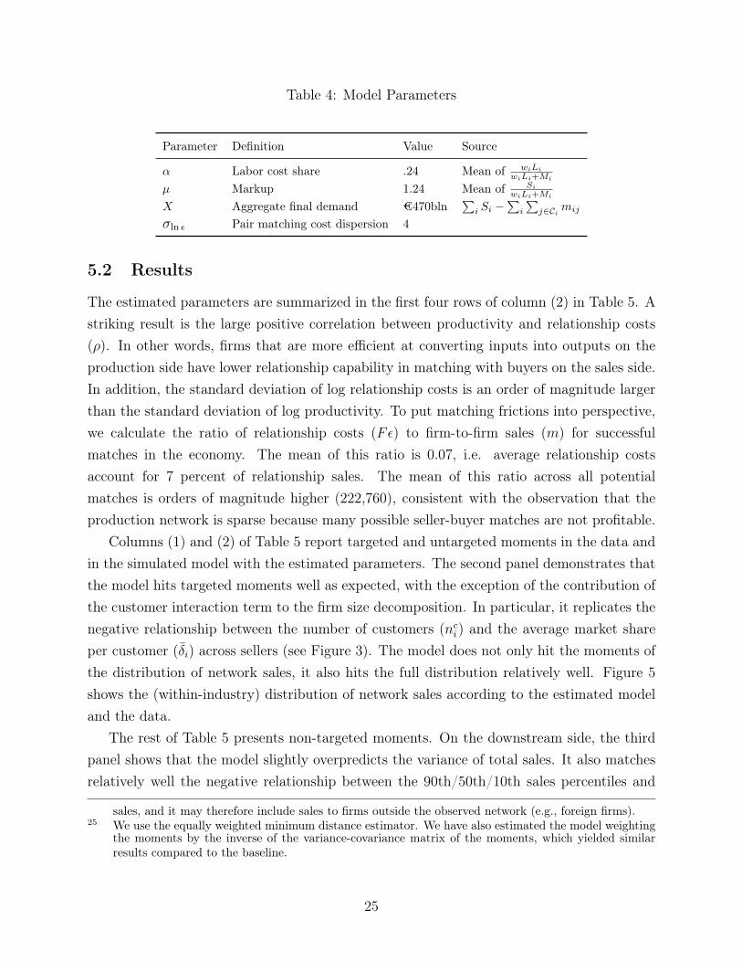
Table 4: Model Parameters

Parameter Definition Value Source

α Labor cost share .24 Mean of wiLi

wiLi+Mi

µ Markup 1.24 Mean of Si

wiLi+Mi

X Aggregate final demand €470bln∑i Si −

∑i

∑j∈Ci mij

σln ε Pair matching cost dispersion 4

5.2 Results

The estimated parameters are summarized in the first four rows of column (2) in Table 5. Astriking result is the large positive correlation between productivity and relationship costs(ρ). In other words, firms that are more efficient at converting inputs into outputs on theproduction side have lower relationship capability in matching with buyers on the sales side.In addition, the standard deviation of log relationship costs is an order of magnitude largerthan the standard deviation of log productivity. To put matching frictions into perspective,we calculate the ratio of relationship costs (Fε) to firm-to-firm sales (m) for successfulmatches in the economy. The mean of this ratio is 0.07, i.e. average relationship costsaccount for 7 percent of relationship sales. The mean of this ratio across all potentialmatches is orders of magnitude higher (222,760), consistent with the observation that theproduction network is sparse because many possible seller-buyer matches are not profitable.

Columns (1) and (2) of Table 5 report targeted and untargeted moments in the data andin the simulated model with the estimated parameters. The second panel demonstrates thatthe model hits targeted moments well as expected, with the exception of the contribution ofthe customer interaction term to the firm size decomposition. In particular, it replicates thenegative relationship between the number of customers (nci) and the average market shareper customer (δi) across sellers (see Figure 3). The model does not only hit the moments ofthe distribution of network sales, it also hits the full distribution relatively well. Figure 5shows the (within-industry) distribution of network sales according to the estimated modeland the data.

The rest of Table 5 presents non-targeted moments. On the downstream side, the thirdpanel shows that the model slightly overpredicts the variance of total sales. It also matchesrelatively well the negative relationship between the 90th/50th/10th sales percentiles and

sales, and it may therefore include sales to firms outside the observed network (e.g., foreign firms).25 We use the equally weighted minimum distance estimator. We have also estimated the model weighting

the moments by the inverse of the variance-covariance matrix of the moments, which yielded similarresults compared to the baseline.

25

Table 5: SMM Model Fit

Data Estimated models(1) (2) Baseline (3) No F (4) No Z (4) No rho

Estimated parameters:µlnF 18.11 (.02) 19.18 (.02) 19.65 (.02) 18.21 (.02)σln z .24 (.00) .13 (.00) .07 (.00)σlnF 2.23 (.01) 1.48 (.01) 1.29 (.01)ρ .86 (.00) 01

Targeted moments:mean (lnnci ) -8.12 -8.12 -8.27 -8.14 -8.12var (lnnci ) 1.87 1.86 0.81 2.20 1.92var (lnSneti ) 3.12 3.12 3.37 2.78 3.08β from ln δi = α+ β lnnci + εi -.11 -.10 1.10 .15 .28Decomp.: # cust. .51 .52 .49 .89 .76Decomp.: Avg cust. capability .05 .01 .01 .03 .02Decomp.: Customer interaction .25 -.04 -.04 -.05 -.06

Non-targeted moments:Downstreamvar (lnSi) 1.73 2.08 1.61 .62 .90var (lnValue Added/Workeri) .62 .71 .15 .54 .42β from lnmk

i = α+ β lnnci + εi -.25/-.28/-.29 -.14/-.15/-.17 1.07/1.06/1.02 .15/.13/.11 .27/.25/.19Downstream degree assort. -.05 -.04 -.07 -.02 -.03

Upstreamvar (lnMnet

i ) 2.12 2.08 1.61 .62 .90var (lnnsi ) .60 .41 .38 .12 .18Upstream degree assort. -.18 -.18 -.07 -.15 -.15

Notes: The number of customers in column (1), nci , is normalized relative to the number of firms in the finalsample. δi is the geometric mean of the market share δij = mij/Mj for seller i across its buyers j. Downstreamdegree assortativity refers to β from the regression for i’s customers lnMeaninsj= α+ β lnnci + εi. Upstream de-gree assortativity refers to β from the regression for j’s suppliers lnMeanjnci= α+ β lnnsj + εj . lnmk

i is the kth(10th/50th/90th) percentile of log bilateral sales, lnmij , for seller i across its customers j. The three decomposi-tion moments refer to the contribution of different margins to firm size dispersion from Section 3. All variables incolumn (1) except mean (lnnci ) are demeaned by NACE 4-digit industry averages. Bootstrapped standard errorsin parentheses.

26

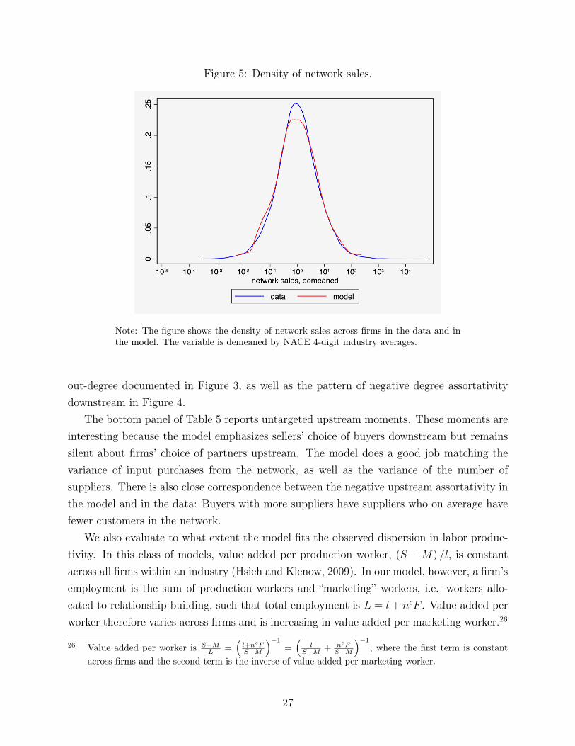
Figure 5: Density of network sales.

Note: The figure shows the density of network sales across firms in the data and inthe model. The variable is demeaned by NACE 4-digit industry averages.

out-degree documented in Figure 3, as well as the pattern of negative degree assortativitydownstream in Figure 4.

The bottom panel of Table 5 reports untargeted upstream moments. These moments areinteresting because the model emphasizes sellers’ choice of buyers downstream but remainssilent about firms’ choice of partners upstream. The model does a good job matching thevariance of input purchases from the network, as well as the variance of the number ofsuppliers. There is also close correspondence between the negative upstream assortativity inthe model and in the data: Buyers with more suppliers have suppliers who on average havefewer customers in the network.

We also evaluate to what extent the model fits the observed dispersion in labor produc-tivity. In this class of models, value added per production worker, (S −M) /l, is constantacross all firms within an industry (Hsieh and Klenow, 2009). In our model, however, a firm’semployment is the sum of production workers and “marketing” workers, i.e. workers allo-cated to relationship building, such that total employment is L = l+ ncF . Value added perworker therefore varies across firms and is increasing in value added per marketing worker.26

26 Value added per worker is S−ML =

(l+ncFS−M

)−1

=(

lS−M + ncF

S−M

)−1

, where the first term is constantacross firms and the second term is the inverse of value added per marketing worker.

27

In equilibrium, firms with high productivity and/or high relationship capability have highervalue added per marketing worker, and therefore also greater labor productivity. Table 5confirms that the estimated model produces significant variance in log labor productivity,although dispersion in the model is slightly higher (.71 versus .62).

5.3 Restricted Models

We next illustrate the need for two firm attributes in order to rationalize observed empiricalpatterns, by estimating a model with heterogeneity in either (i) productivity (“no F”) or(ii) relationship capability (“no Z”) but not both. Under (i), there are two parameters toestimate, Υ = σln z, µlnF, and we use the same moments to identify Υ. Under (ii), theparameters to estimate are Υ = µlnF , σlnF.

The estimated parameters and fit of these two restricted models are summarized incolumns (3) and (4) of Table 5. Both restricted models are unable to generate the neg-ative correlation between the average market share (δi) and the number of customers acrosssellers (the β coefficient from the regression ln δi = α + β lnnci + εi). Figure 6 plots this rela-tionship according to the estimated restricted models. In both cases, the model generatesthe opposite pattern to the empirical regularity in Figure 3.

In addition, the single factor models do a relatively poor job in other dimensions. In the“noF” case, we more or less match dispersion in network sales, but this comes at the expenseof not matching the variance in the number of customers or in value added per worker. Inthe “noZ” case, we match dispersion in the number of customers, but dispersion in total salesis too small, and the contribution of the number of customers in the firm size decompositionis too high. Both restricted models underestimate the variances of input purchases and ofthe number of suppliers, and counterfactually imply that bilateral sales at different customerpercentiles increase rather than decrease with the number of customers.

Finally, we estimate a model with heterogeneity in both productivity and relationshipcapability, but where the correlation between them set to zero, ρ = 0 (“no rho”). The lastcolumn of Table 5 shows that the restricted model produces a positive correlation betweenaverage market share (δi) and the number of customers across sellers (the slope coefficientis .28), far from the slightly negative coefficient in the data. Furthermore, it does poorly formany non-targeted moments: the restricted model generates significantly less heterogeneityin both log sales, log input purchases and log number of suppliers. This result highlightsthat a data-generating process with unrelated Z and F is inconsistent with our data.

28

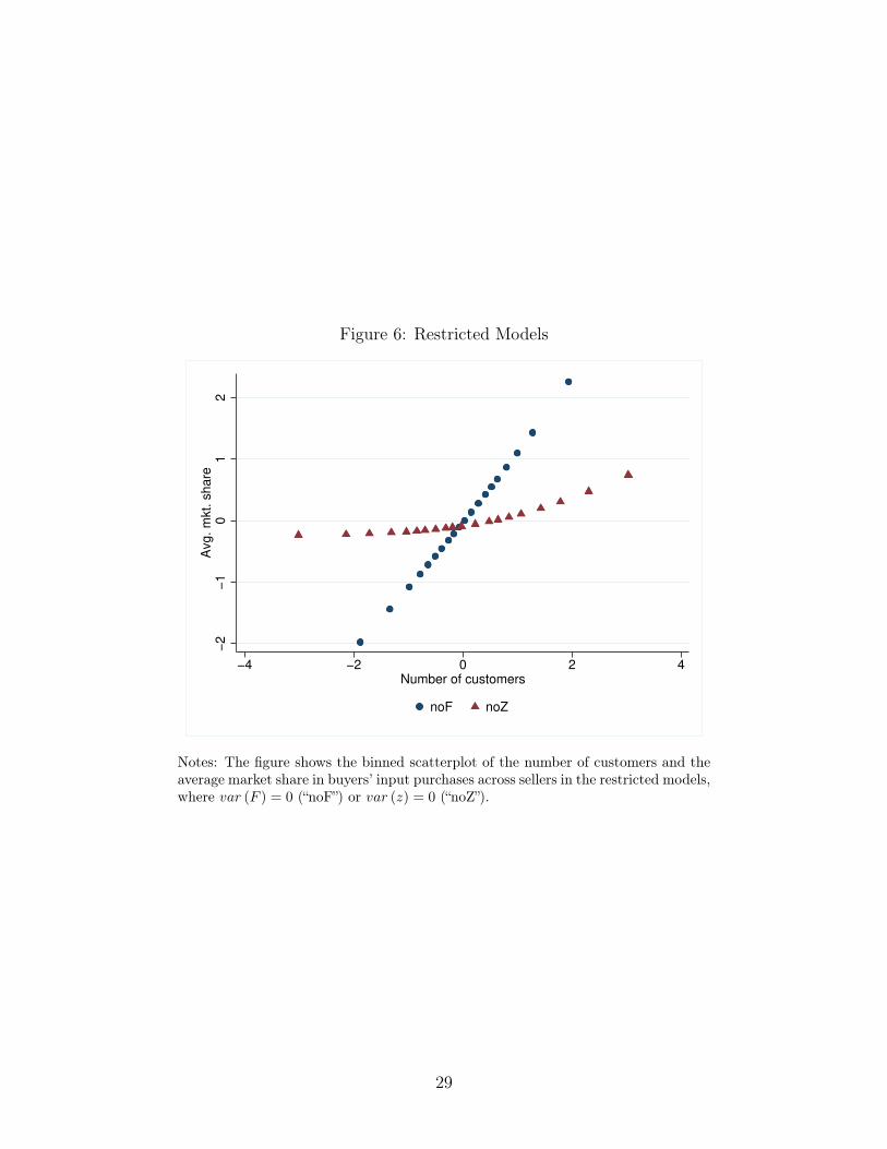
Figure 6: Restricted Models

−2

−1

01

2A

vg. m

kt. s

hare

−4 −2 0 2 4Number of customers

noF noZ

Notes: The figure shows the binned scatterplot of the number of customers and theaverage market share in buyers’ input purchases across sellers in the restricted models,where var (F ) = 0 (“noF”) or var (z) = 0 (“noZ”).

29

5.4 Sensitivity

Next, we evaluate the sensitivity of the estimates to the vector of estimation moments. Weuse the methodology from Andrews et al. (2017). Specifically, we ask how sensitive theparameter estimate ρ (the correlation between productivity and relationship costs) is to per-turbations of the various moments of the data. We consider perturbations that are additiveshifts of the moment functions due to either misspecification of xs (Υ) or measurement errorin the empirical moments x. Andrews et al. (2017) show that sensitivity can be summarizedby the matrix Λ = (S ′WS)−1 S ′W , where S is the matrix of partial derivatives of xs (Υ)

evaluated at the true value Υ0 (see their Proposition 2). W is the method of momentsweighting matrix, which in our case is the identity matrix.

Figure 7 plots the column of the estimated Λ corresponding to the parameter estimateρ. The plot shows one-hundredth of the value of sensitivity of the parameter ρ with respectto the vector of estimation moments. The values are scaled by the standard deviation of themoments, so the values can be interpreted as the effect of a one standard deviation change inthe moment on the parameter ρ. The plot largely confirms our intuition about identification.First, the slope coefficient β (from the regression of average market share on the number ofcustomers) is the moment that matters the most, while the other moments are less relevantfor this particular parameter. Furthermore, the direction of sensitivity is also in line withour expectations: A steeper slope coefficient has a negative impact on ρ, i.e. we get a lowerpositive correlation between Z and F as the slope becomes steeper.

5.5 A Counterfactual

We end this section by quantifying the role of firm heterogeneity in productivity and re-lationship costs for aggregate outcomes. We do so by performing a simple counterfactualexperiment: a common 50 percent reduction in relationship costs across all firms in theeconomy (i.e. a reduction in µlnF ). We do so both in the baseline estimated model and ina restricted model with no correlation between productivity and relationship costs, in orderto illustrate the importance of the latter.

The simulation shows that real wages increase by 17% in the baseline and 12% in themodel with no correlation, which implies that the welfare gains are 42% higher with correla-tion than without. Figure 8 shows a binned scatterplot of the counterfactual change in thelog number of customers on the vertical axis against log productivity (lnZ) on the horizontalaxis. The solid circles refer to the baseline counterfactual, while the triangles denote the no-correlation counterfactual. In both versions of the model, lower relationship costs generatemany new customers per firm. In the baseline model, the increase is relatively similar across

30

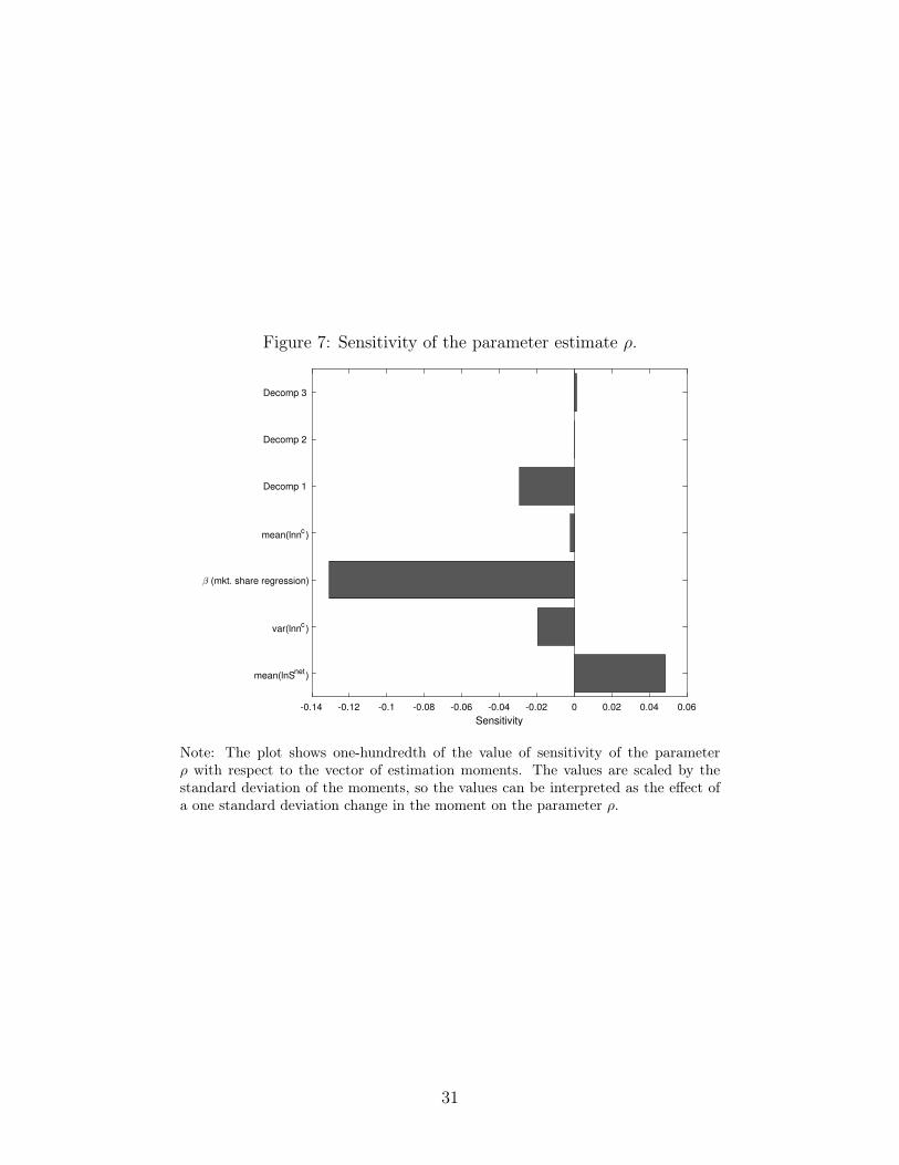
Figure 7: Sensitivity of the parameter estimate ρ.

-0.14 -0.12 -0.1 -0.08 -0.06 -0.04 -0.02 0 0.02 0.04 0.06

Sensitivity

mean(lnSnet

)

var(lnnc)

(mkt. share regression)

mean(lnnc)

Decomp 1

Decomp 2

Decomp 3

Note: The plot shows one-hundredth of the value of sensitivity of the parameterρ with respect to the vector of estimation moments. The values are scaled by thestandard deviation of the moments, so the values can be interpreted as the effect ofa one standard deviation change in the moment on the parameter ρ.

31

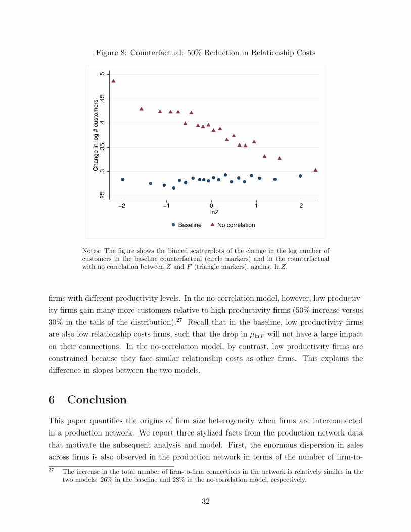
Figure 8: Counterfactual: 50% Reduction in Relationship Costs

.25

.3.3

5.4

.45

.5C

hange in log #

custo

mers

−2 −1 0 1 2lnZ

Baseline No correlation

Notes: The figure shows the binned scatterplots of the change in the log number ofcustomers in the baseline counterfactual (circle markers) and in the counterfactualwith no correlation between Z and F (triangle markers), against lnZ.

firms with different productivity levels. In the no-correlation model, however, low productiv-ity firms gain many more customers relative to high productivity firms (50% increase versus30% in the tails of the distribution).27 Recall that in the baseline, low productivity firmsare also low relationship costs firms, such that the drop in µlnF will not have a large impacton their connections. In the no-correlation model, by contrast, low productivity firms areconstrained because they face similar relationship costs as other firms. This explains thedifference in slopes between the two models.

6 Conclusion

This paper quantifies the origins of firm size heterogeneity when firms are interconnectedin a production network. We report three stylized facts from the production network datathat motivate the subsequent analysis and model. First, the enormous dispersion in salesacross firms is also observed in the production network in terms of the number of firm-to-27 The increase in the total number of firm-to-firm connections in the network is relatively similar in the

two models: 26% in the baseline and 28% in the no-correlation model, respectively.

32

firm connections and the value of pairwise sales. Second, firms with higher sales have morecustomers but lower average sales per customer and lower market shares (of input purchases)among their customers. Finally, there is negative degree assortativity between buyers andsuppliers, i.e. sellers with more customers match with customers who have fewer supplierson average.

Taken together, these facts present challenges to many existing models of firm hetero-geneity. The large variation in sales across firms within an industry is intuitively related tovariation in the number of customers: larger firms have more customers. However, largerfirms also sell less to their customers. Models that emphasize heterogeneity in productivityacross firms cannot explain these facts simultaneously. In particular, such models imply thatfirms with more customers should also sell more to each of their customers and have higherrather than lower market shares.

We confirm the importance of the production network in a decomposition of the varianceof firm sales within narrowly defined industries. 81% of the variation in firm sales is associatedwith the downstream component, and most of that is due to variation in the number ofcustomers. The upstream component contributes 18%, and variation in the share of salesoutside the domestic production network plays a minor role at 1%. These findings implythat trade in intermediate goods and the number of firm-to-firm connections are essential tounderstanding firm performance and, consequently, aggregate outcomes.

Motivated by the stylized facts and decomposition results, we develop a quantitativegeneral-equilibrium model of firm-to-firm trade. In the model, firms differ along two dimen-sions – productivity and relationship capability – defined respectively as production efficiencyand (the inverse of) the fixed cost of matching with a customer. Suppliers match with cus-tomers if the gross profits from the match exceed the supplier-specific fixed matching cost.Marginal costs, employment, prices, and sales are endogenous outcomes because they dependon the outcomes of all other firms in the economy. A link between two firms increases thetotal sales of both the seller and the buyer; for the seller this occurs mechanically becauseit gains a customer, while for the buyer this arises because a larger supplier base lowers themarginal cost of production.

We estimate parameters of the model using simulated method of moments. The resultsreveal a strong negative correlation between the two firm characteristics: Firms with higherproductivity have lower relationship capability. Importantly, both dimensions of firm het-erogeneity are necessary to match the data. Shutting down one at a time results in poormodel fit, including the inability to replicate the negative relationship between the numberof customers and average sales per customer.

Our results challenge current understanding of the sources of firm size heterogeneity,

33

and point to important areas for future research on the negative relationship between firmproductivity and relationship capability. While we make progress in matching the relativeimportance of upstream and downstream factors in firm success, there is room for new mod-els to better fit these features of the production network. In addition, research is neededto examine the factors that lead to a negative relationship between productivity and rela-tionship capability across firms. One promising avenue for further work is examining spanof control issues inside the firm and the allocation of resources to improving productivityversus acquiring more customers.

34

References

Abowd, J.M., F. Kramarz, and D.N. Margolis, “High Wage Workers and High WageFirms,” Econometrica, 1999, 67 (2), 251–333. 3, 3.1, 14, C.2

Acemoglu, Daron, Vasco M. Carvalho, Asuman Ozdaglar, and Alireza Tahbaz-Salehi, “The Network Origins of Aggregate Fluctuations,” Econometrica, 2012, 80 (5),1977–2016. 1

Allen, Treb, Costas Arkolakis, and Xiangliang Li, “On the Existence and Uniquenessof Trade Equilibria,” Technical Report, Working paper 2016. D.3

Andrews, Isaiah, Matthew Gentzkow, and Jesse M. Shapiro, “Measuring the Sen-sitivity of Parameter Estimates to Estimation Moments,” The Quarterly Journal of Eco-nomics, 2017, 132 (4), 1553–1592. 5.4

Antràs, P., T.C. Fort, and F. Tintelnot, “The Margins of Global Sourcing: Theory andEvidence from US Firms,” American Economic Review, September 2017, 107 (9), 2514–64.1, 4.5

Arkolakis, Costas, “Market Penetration Costs and the New Consumers Margin in Inter-national Trade,” Journal of Political Economy, 2010, 118 (6). 2.2

Autor, David, David Dorn, Lawrence F. Katz, Christina Patterson, and John VanReenen, “The Fall of the Labor Share and the Rise of Superstar Firms,” Quarterly Journalof Economics, 2020, 135 (2), 645–709. 1

Baqaee, David Rezza and Emmanuel Farhi, “The Macroeconomic Impact of Microe-conomic Shocks: Beyond Hulten’s Theorem,” Econometrica, 2019, 87 (4), 1155–1203. 1

and , “Productivity and Misallocation in General Equilibrium,” Quarterly Journal ofEconomics, 2020, 135 (1), 105–163. 1

Bender, S., D. Card, N. Bloom, J. Van Reenen, and S. Wolter, “ManagementPractices, Workforce Selection and Productivity,” Journal of Labor Economics, January2018, 36 (1), S371–S409. 1

Bernard, A., A. Moxnes, and Y.U. Saito, “Production Networks, Geography and FirmPerformance,” Journal of Political Economy, 2019. 1, 8, 12

35

Bernard, A.B., J.B. Jensen, S.J. Redding, and P.K. Schott, “The Empirics of FirmHeterogeneity and International Trade,” Annual Review of Economics, 2012, 4 (1), 283–313. 1

Bernard, Andrew B. and Andreas Moxnes, “Networks and Trade,” Annual Review ofEconomics, August 2018, 10, 65–85. 1

, , and Karen Helene Ulltveit-Moe, “Two-sided Heterogeneity and Trade,” Reviewof Economics and Statistics, 2018, 100 (3). 1, 8, 2.2, 12, 4.4

, Emmanuel Dhyne, Glenn Magerman, Kalina Manova, and Andreas Moxnes,“The Origins of Firm Heterogeneity: A Production Network Approach,” Technical Report25441, NBER Working paper 25441 2018. 21

Bloom, Nick, Kalina Manova, John Van Reenen, Stephen Sun, and Zhihong Yu,“Managing Trade: Evidence from China and the US,” NBER Working Paper 24718., 2017.1

Boehm, Johannes and Ezra Oberfield, “Misallocation in the Market for Inputs: En-forcement and the Organization of Production,” Quarterly Journal of Economics, 2020,135 (4), 2007–2058. 1

Bøler, Esther Ann, Andreas Moxnes, and Karen Helene Ulltveit-Moe, “R&D,International Sourcing, and the Joint Impact on Firm Performance,” American EconomicReview, 2015, 105 (12). 1

Bonhomme, Stéphane, “Econometric Analysis of Bipartite Networks,” in B. Graham andA. de Paula, eds., The Econometric Analysis of Network Data, Academic Press, 2020. 32

Card, D., J. Heining, and P. Kline, “Workplace Heterogeneity and the Rise of WestGerman Wage Inequality*,” The Quarterly Journal of Economics, 2013, 128 (3), 967–1015. C.2, 34

Correia, Sergio, “Linear Models with High-Dimensional Fixed Effects: An Efficient andFeasible Estimator,” Technical Report, Working Paper 2016. 1

Dhyne, E., G. Magerman, and S. Rubinova, “The Belgian Production Network 2002-2012,” National Bank of Belgium Working Paper, 2015, 288. 2.1, 8, A.1

di Giovanni, J., A.A. Levchenko, and I. Mejean, “Firms, Destinations, and AggregateFluctuations,” Econometrica, 07 2014, 82 (4), 1303–1340. 1

36

Eaton, J., D. Jinkins, J. Tybout, and D.Y. Xu, “Two-sided Search in InternationalMarkets,” 2016. NBER. 1

, S. Kortum, and F. Kramarz, “Dissecting Trade: Firms, Industries, and ExportDestinations,” American Economic Review, May 2004, 94 (2), 150–154. 3.1

Eaton, Jonathan, Samuel Kortum, and Francis Kramarz, “Firm-to-Firm Trade: Im-ports, Exports, and the Labor Market1,” Technical Report, Working paper 2018. 1, 2.2

Fieler, Ana Cecília, Marcela Eslava, and Daniel Yi Xu, “Trade, Quality Upgrad-ing, and Input Linkages: A Theory with Evidence from Colombia,” American EconomicReview, 2018, 108. 1

Fitzgerald, D., S. Haller, and Y. Yedid-Levi, “How Exporters Grow,” Staff Report524, Federal Reserve Bank of Minneapolis January 2016. 1

Foster, L., J. Haltiwanger, and C. Syverson, “The Slow Growth of New Plants: Learn-ing about Demand?,” Economica, 2016, 83 (329), 91–129. 1

Freund, C. and M.D. Pierola, “Export Superstars,” The Review of Economics and Statis-tics, 2015, 97 (5), 1023–1032. 1

Gabaix, Xavier, “The Granular Origins of Aggregate Fluctuations,” Econometrica, 2011,79, 733–772. 1

Gaubert, Cecile and Oleg Itskhoki, “Granular Comparative Advantage,” Journal ofPolitical Economy, March 2021, 129 (3), 871–939. 1

Gibrat, Robert, Les inègalitès èconomiques, Librairie du Recuil Sirey, Paris, 1931. 1

Goldberg, P., A.K. Khandelwal, N. Pavcnik, and P. Topalova, “Imported Intermedi-ate Inputs and Domestic Product Growth: Evidence from India,” The Quarterly Journalof Economics, 2010, 125 (4), 1727–1767. 1

Holmstrom, Bengt and Paul Milgrom, “Multitask Principal-Agent Analyses: IncentiveContracts, Asset Ownership, and Job Design,” Journal of Law, Economics, and Organi-zation, 1991, 7, 24–52. 1

Hong, Fuhai, Tanjim Hossain, John A. List, and Migiwa Tanaka, “Testing theTheory of Multitasking: Evidence From a Natural Field Experiment in Chinese Factories,”International Economic Review, 2018, 59 (2), 511–536. 4

37

Hopenhayn, H.A., “Entry, Exit and Firm Dynamics in Long Run Equilibrium,” Econo-metrica, 1992, 60, 1127–1150. 1

Hottman, C. J., S.J. Redding, and D. E. Weinstein, “Quantifying the Sources of FirmHeterogeneity,” Quarterly Journal of Economics, 2016, 131 (3), 1291–1364. 1, 3.1

Hsieh, Chang-Tai and Peter J. Klenow, “Misallocation and Manufacturing TFP inChina and India,” The Quarterly Journal of Economics, 2009, 124 (4). 5.2

Jovanovic, Boyan, “Selection and the Evolution of Industry,” Econometrica, May 1982, 50(3), 649–70. 1

Lim, Kevin, “Endogenous Production Networks and the Business Cycle,” Technical Report2018. 1, 2.2, 12, 4.4

Luttmer, Erzo G. J., “Selection, growth and the size distribution of firms,” The QuarterlyJournal of Economics, 2007, 78 (3), 1042–1068. 1

, “On The Mechanics of Firm Growth,” The Review of Economic Studies, 2011, 122 (3),1103–1144. 1

Magerman, Glenn, Karolien De Bruyne, Emmanuel Dhyne, and Jan Van Hove,“Heterogeneous Firms and the Micro Origins of Aggregate Fluctuations,” Technical Report,KU Leuven 2016. 1

Manova, Kalina, Shang-Jin Wei, and Zhiwei Zhang, “Firm Exports and MultinationalActivity Under Credit Constraints,” The Review of Economics and Statistics, July 2015,97 (3), 574–588. 1

McFadden, Daniel, “A method of simulated moments for estimation of discrete responsemodels without numerical integration,” Econometrica, 1989, 57, 995–1026. 23

Melitz, Marc., “The Impact of Trade on Intra-Industry Reallocations and Aggregate In-dustry,” Econometrica, 2003, 71 (6), 1695–1725. 1

Melitz, Marc and Stephen Redding, “New Trade Models, New Welfare Implications,”American Economic Review, 2015, 105 (3), 1105–1146. 1

Oberfield, Ezra, “A Theory of Input-Output Architecture,” Econometrica, 2018, 86 (2),559–589. 1

Pavcnik, Nina, “Trade Liberalization, Exit, and Productivity Improvements: Evidencefrom Chilean Plants,” The Review of Ecnomic Studies, 2002, 69, 245–276. 1

38

Prescott, Edward C. and Michael Visscher, “Organizational Capital,” The Journal ofPolitical Economy, June 1980, 88 (3), 446–461. 1

Sutton, John, “Market Share Dynamics and the "Persistence of Leadership" Debate,”American Economic Review, March 2007, 97 (1), 222–241. 1

Syverson, C., “What Determines Productivity?,” Journal of Economic Literature, 2011, 49(2), 326–365. 1

Tintelnot, Felix, Ken Kikkawa, Magne Mogstad, and Emmanuel Dhyne, “Tradeand Domestic Production Networks,” Review of Economic Studies, 2021, 88 (2), 643–668.1, E.6

39

Appendix

A Data Sources

A.1 Data sources

The empirical analysis draws on four micro-level datasets at the National Bank of Belgium(NBB), covering the period 2002-2014: (i) the NBB B2B Transactions Dataset, (ii) annualaccounts from the Central Balance Sheet Office supplemented by (iii) VAT declarations, and(iv) the Crossroads Bank. Firms are identified by a unique enterprise number, which iscommon across all databases and allows for unambiguous merging.

Firm-to-firm relationships The confidential NBB B2B Transactions Dataset contains thevalue of yearly sales among all VAT-liable Belgian enterprises for the years 2002 to 2014,and is based on the VAT listings collected by the tax authorities. All firms that delivergoods or services as an economic activity, on a regular and independent basis, are VATliable. These enterprises have to charge an ad valorem tax on their sales and can recoverVAT paid on their purchases. This includes foreign companies with a branch in Belgium andfirms whose securities are officially listed in Belgium. Enterprises that only perform financialtransactions, medical or socio-cultural activities such as education are exempt. Firms withsales less than €15,000 can choose to be exempt from the VAT liabilities. The standardVAT rate in Belgium is 21%, but for some goods a reduced rate of 12% or 6% applies.28

At the end of every calendar year, all VAT-liable enterprises have to file a complete listing oftheir Belgian VAT-liable customers over that year. An observation in this dataset refers tothe value of sales in euro by enterprise i to enterprise j within Belgium, excluding the VATdue on these sales. The reported value is the sum of invoices from i to j in a given calendaryear. Whenever this aggregated value is €250 or greater, the relationship has to be reported.Together with the VAT declarations, these listings are the basis for the VAT amount dueper tax period. Fines for late or incomplete reporting ensure a very high quality of the data.Note that each relationship is directed, as the observation from i to j is different from anobservation from j to i. The dataset thus covers both the extensive and the intensive marginsof the Belgian production network. A detailed description of the collection and cleaning ofthis dataset is given in Dhyne et al. (2015). We refer to that paper for further details.

Firm characteristics We extract information on enterprises’ annual accounts from the28 See ec.europa.eu/taxation_customs for a complete list of rates. These rates did not change over our

sample period.

40

Central Balance Sheet Office at the NBB for the years 2002 to 2014. Enterprises above acertain size threshold have to file annual accounts at the end of their fiscal year. We retaininformation on the enterprise identifier (VAT ID), turnover (total sales in euro, code 70 inthe annual accounts), input purchases (total material and services inputs in euro and netchanges in input stocks, codes 60+61), labor cost (total cost of wages, social securities andpensions in euro, code 62), and employment (average number of full-time equivalent (FTE)employees, code 9087). We annualize all flow variables from fiscal years to calendar years bypro-rating the variables on a monthly basis.29

Enterprises below a size threshold can report abbreviated annual accounts. These firmsstill report labor cost and employment, but are not required to report turnover or inputpurchases. For these small enterprises, we supplement information on turnover and inputexpenditures from their VAT declarations. All VAT-liable enterprises have to file periodicVAT declarations with the tax administration. The VAT declaration contains the totalsales value (including domestic sales and exports), the VAT amount charged on those sales(both to other enterprises and to final consumers), the total amount paid for inputs sourced(including domestic and imported inputs), and the VAT paid on those input purchases. Thisdeclaration is due monthly or quarterly depending on firm size, and it is the basis for theVAT due to the tax authorities every period. We aggregate the VAT declarations to theannual frequency to match the annual accounts.We obtain information on the main economic activity of each enterprise at the NACE 4-digitlevel from the Crossroads Bank of Belgium for the years 2002 to 2014. We concord NACEcodes over time to the NACE Rev. 2 version to deal with changes in the NACE classificationover our panel from Rev. 1.1 to Rev. 2. Table 6 lists industry groups at the NACE 2-digitlevel. Finally, we also retrieve the postal code of the main establishment of the firm from theCrossroads Bank of Belgium. There are 589 municipalities in Belgium, which correspond tothe Local Administrative Units level 2.

Since total sales and network sales come from different datasets, we enforce:

Si = Sneti + fdi

where final demand fdi ≥ 0. For observations where Sneti from the NBB B2B transactionsdataset is larger than Si, we replace Si = max(Si, Sneti). This amounts to 6% of observationsin our estimation sample. The median value of Sneti that overshoots Si is 17% of the valuereported in the annual accounts for these observations, before we correct them.29 In our data, 78% of firms have annual accounts that coincide with calendar years, while 98% of firms

have fiscal years of 12 months.

41

Table6:

NACE

classificationof

indu

stry

grou

ps(N

ACE

Rev

2)

NACE

Section

NACE

Division

Description

Indu

stry

ANACE

01-03

Agriculture,forestry

andfishing

Primaryan

dExtraction

BNACE

05-09

Miningan

dqu

arrying

Primaryan

dExtraction

CNACE

10-33

Man

ufacturing

Man

ufacturing

DNACE

35Electricity,gas,

steam

andaircond

itioning

supp

lyUtilities

ENACE

36-39

Water

supp

ly;sewage,

waste

man

agem

entan

dremediation

activities

Utilities

FNACE

41-43

Con

struction

Con

struction

GNACE

45-47

Who

lesale

andretailtrad

e;repa

irof

motor

vehicles

andmotorcycles

MarketServices

HNACE

49-53

Transpo

rtationan

dstorage

MarketServices

INACE

55-56

Accom

mod

ationan

dfood

serviceactivities

MarketServices

JNACE

58-63

Inform

ationan

dcommun

ication

MarketServices

KNACE

64-66

Finan

cial

andinsuranceactivities

MarketServices

LNACE

68Realestate

activities

MarketServices

MNACE

69-75

Professiona

l,scientifican

dtechnicalactivities

MarketServices

NNACE

77-82

Adm

inistrativean

dsupp

ortserviceactivities

MarketServices

ONACE

84Pub

licad

ministrationan

ddefence;

compu

lsorysocial

security

Non

-MarketServices

PNACE

85Edu

cation

Non

-MarketServices

QNACE

86-88

Hum

anhealth

andsocial

workactivities

Non

-MarketServices

RNACE

90-93

Arts,

entertainm

entan

drecreation

Non

-MarketServices

SNACE

94-96

Other

serviceactivities

Non

-MarketServices

TNACE

97-98

Activitiesof

households

asem

ployers;

undiffe

rentiatedgo

ods-

and

–services-produ

cing

activities

ofho

useholds

forow

nuse

UNACE

99Activitiesof

extraterritorial

organization

san

dbo

dies

–

42

lnSi lnnci lnnsivariance 1.73 1.87 0.60skewness 0.57 0.13 -0.02kurtosis 4.54 3.45 4.17

p1 -2.88 -3.18 -2.04p5 -1.93 -2.22 -1.26p10 -1.50 -1.71 -0.93p25 -0.84 -0.89 -0.46p50 -0.11 -0.01 -0.00p75 0.72 0.87 0.46p90 1.66 1.72 0.93p95 2.34 2.25 1.26p99 3.82 3.41 1.97

Table 7: Moments of distributions.Notes: all variables are demeaned by their NACE 4-digit industries by regressing log

variables on sector fixed effects and retaining the residuals.

B Additional results: Stylized facts

B.1 Distributions of firm size and number of connections

We provide additional moments on the distribution of firm sizes and the number of customersand suppliers in Table 7. Again, all variables are in logs, and demeaned by their NACE 4-digit industries.

We also report information on the raw (non-demeaned) distributions of these variables,confirming that massive heterogeneity in the production network is not driven by particularsectors, but instead is natural across all types of economic activity. Table 8 reports thedistribution of firm size in the full sample, as well as separately for six aggregated industriesfor the year 2014: primary and extraction, manufacturing, utilities, construction, marketservices and non-market services. Tables 9 and 10 report summary statistics for the numberof firm customers and the number of firm suppliers, respectively. While there is naturalvariation in average values across different types of economic activity, sizable dispersion isprevalent in all industries.

B.2 Market share and number of customers: seller-buyer sector-

pair demeaning

A potential concern in interpreting the stylized facts in Section 2.2, in particular the rela-tionship between average market shares and number of customers, is that firms with many

43

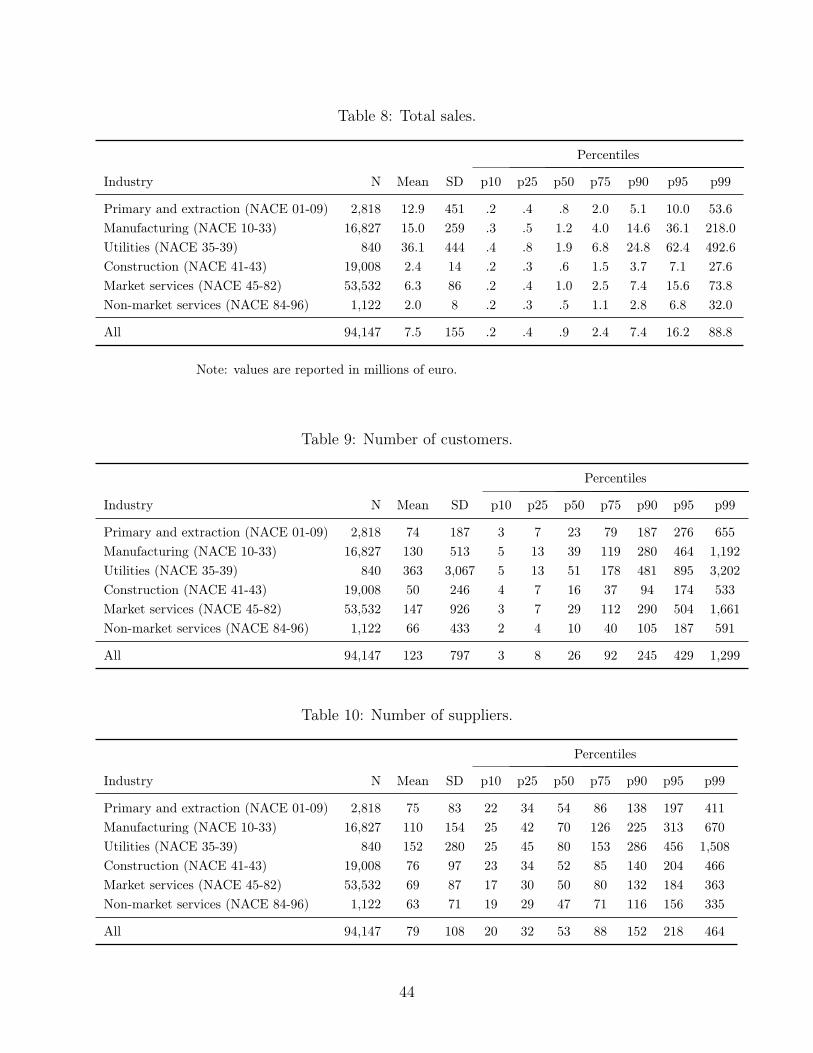
Table 8: Total sales.

Percentiles

Industry N Mean SD p10 p25 p50 p75 p90 p95 p99

Primary and extraction (NACE 01-09) 2,818 12.9 451 .2 .4 .8 2.0 5.1 10.0 53.6Manufacturing (NACE 10-33) 16,827 15.0 259 .3 .5 1.2 4.0 14.6 36.1 218.0Utilities (NACE 35-39) 840 36.1 444 .4 .8 1.9 6.8 24.8 62.4 492.6Construction (NACE 41-43) 19,008 2.4 14 .2 .3 .6 1.5 3.7 7.1 27.6Market services (NACE 45-82) 53,532 6.3 86 .2 .4 1.0 2.5 7.4 15.6 73.8Non-market services (NACE 84-96) 1,122 2.0 8 .2 .3 .5 1.1 2.8 6.8 32.0

All 94,147 7.5 155 .2 .4 .9 2.4 7.4 16.2 88.8

Note: values are reported in millions of euro.

Table 9: Number of customers.

Percentiles

Industry N Mean SD p10 p25 p50 p75 p90 p95 p99

Primary and extraction (NACE 01-09) 2,818 74 187 3 7 23 79 187 276 655Manufacturing (NACE 10-33) 16,827 130 513 5 13 39 119 280 464 1,192Utilities (NACE 35-39) 840 363 3,067 5 13 51 178 481 895 3,202Construction (NACE 41-43) 19,008 50 246 4 7 16 37 94 174 533Market services (NACE 45-82) 53,532 147 926 3 7 29 112 290 504 1,661Non-market services (NACE 84-96) 1,122 66 433 2 4 10 40 105 187 591

All 94,147 123 797 3 8 26 92 245 429 1,299

Table 10: Number of suppliers.

Percentiles

Industry N Mean SD p10 p25 p50 p75 p90 p95 p99

Primary and extraction (NACE 01-09) 2,818 75 83 22 34 54 86 138 197 411Manufacturing (NACE 10-33) 16,827 110 154 25 42 70 126 225 313 670Utilities (NACE 35-39) 840 152 280 25 45 80 153 286 456 1,508Construction (NACE 41-43) 19,008 76 97 23 34 52 85 140 204 466Market services (NACE 45-82) 53,532 69 87 17 30 50 80 132 184 363Non-market services (NACE 84-96) 1,122 63 71 19 29 47 71 116 156 335

All 94,147 79 108 20 32 53 88 152 218 464

44

customers might be selling different types of products compared to firms with few customers,even within the same 4-digit industry of the seller. In that case, average market shares mightdepend on seller-buyer pair characteristics, rather than characteristics of the seller only. Forexample, there may be both niche and broad-market sellers within the same industry, wherethe broad seller has more customers than the niche seller. Presumably, buyers of niche andbroad-market products to some extent also belong to different industries: e.g. broad-marketcoffee roasters may sell to grocery stores, while niche coffee roasters may sell to coffee shops.

To take this into account, we reproduce the correlation between customer market sharesand the number of customers in Fact 2, using fixed effects for the seller-buyer industrypair. By also demeaning by the customer sector, we account for heterogeneity in inputrequirements across sectors within the sector of the supplier. Specifically, for every seller i,we calculate the average market share and the number of customers in each 4-digit buyerindustry k, δik and nik, respectively. The average market share is calculated as in themain text: the weighted geometric mean of mij/M

netj across customers j belonging to buyer

industry k. We then regress δik on nik (in logs), including seller-buyer industry pair fixedeffects. The OLS slope coefficient remains negative and significant at -.03. While part ofthe variation is indeed absorbed by sector-pair-specific components, this shows that, evenwhen looking at sales within a very detailed cell of the input-output table, e.g. coffee roastersselling to coffee shops, sellers with many customers obtain systematically lower market sharesof their buyers’ input purchases.

B.3 Fringe buyers

Another potential concern is that sellers with many connections have relatively more fringebuyers than firms with fewer connections, i.e. less important customers in terms of bilateralsales mij. This pattern would imply that firms with more customers have lower average salesper customer and lower market shares in these customers, but higher sales to each customerat each customer rank, rejecting the model in the main text.

We investigate this possibility by looking at the relationship between firm sales andthe number of customers after dropping potential fringe buyers. We identify and drop fringebuyers in two ways. First, we drop transactionsmij that are below the first quartile of a firm’stransactionsmij (i.e., the quartile is firm-specific).30 Alternatively, we drop transactions thatare below the global 1st quartile across all mij in the sample. In each case we recalculatethe adjusted number of customers nci and network sales Sneti . Table 11 repeats the baselineanalysis in this modified sample. The first column reproduces the baseline results for the30 This means that the analysis is restricted to firms with 5 or more customers.

45

Dep. var: lnSneti (1) Baseline (2) No fringe buyers (firm-level) (2) No fringe buyers (global)lnnci .77∗∗∗ .81∗∗∗ .91∗∗∗

(.00) (.01) (.00)Seller industry fixed effects Yes Yes Yes

N 94,147 80,224 80,156

Table 11: Fringe buyers, 2014.

Note: Regressions comparing the elasticity of sales with respect to the number of customers across (1)baseline, (2) after dropping fringe buyers (bottom quartile) within each firm, and (3) after droppingfringe buyers (bottom quartile) across all firms. Significance: * < 5%, ** < 1%, *** <0.1%.

regression of lnSneti on lnnci , while columns 2 and 3 show the results after removing fringebuyers. The slope coefficient increases slightly, but the main message of Fact 2 remains,namely that average sales (and market shares) are smaller for firms with many customers.

C Exogenous mobility

In this section, we first discuss the empirical relevance of buyer and seller effects in equa-tion (1). We then examine the necessary assumptions on the assignment process of buyersand sellers for OLS to identify the underlying parameters of interest, and develop a simpleevaluation of conditional exogenous mobility in the context of a production network.

C.1 Buyer and seller effects

The log-linear relationship in equation (1) predicts the following: (i) expected sales fromseller i to customer j are increasing in the average sales of i to other customers k, and (ii)expected purchases by buyer j from seller i are increasing in the average purchases by j fromother suppliers k.

Both properties can be tested non-parametrically as follows. For each seller i and buyerj, calculate the leave-out mean of log sales (s−li ) and purchases (m−lj ) across its buyers and

46

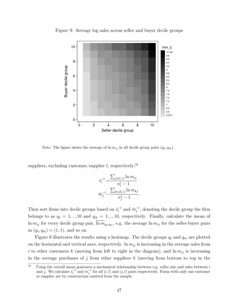
Figure 9: Average log sales across seller and buyer decile groups

0

2

4

6

8

10

Buyer

decile

gro

up

0 2 4 6 8 10

Seller decile group

10.182

9.8

9.6

9.4

9.2

9

8.8

8.6

8.4

8.2

8

7.8

7.6

7.4

7.2

7

6.8

6.6

6.3911

lnm_ij

Note: The figure shows the average of lnmij in all decile group pairs (qs, qm).

suppliers, excluding customer/supplier l, respectively:31

s−li =

∑j∈Ci\l lnmij

nci − 1

m−lj =

∑k∈Sj\l lnmkj

nsj − 1.

Then sort firms into decile groups based on s−li and m−lj , denoting the decile group the firmbelongs to as qs = 1, .., 10 and qm = 1, .., 10, respectively. Finally, calculate the mean oflnmij for every decile group pair, lnmqs,qm , e.g. the average lnmij for the seller-buyer pairsin (qs, qm) = (1, 1), and so on.

Figure 9 illustrates the results using a heatmap. The decile groups qs and qm are plottedon the horizontal and vertical axes, respectively. lnmij is increasing in the average sales fromi to other customers k (moving from left to right in the diagram), and lnmij is increasingin the average purchases of j from other suppliers k (moving from bottom to top in the31 Using the overall mean generates a mechanical relationship between e.g. seller size and sales between i

and j. We calculate s−li and m−lj for all (i, l) and (j, l) pairs respectively. Firms with only one customeror supplier are by construction omitted from the sample.

47

diagram).

C.2 Assumptions on the Assignment Process

Equation (1) is a two-way fixed effects model similar to the models that are used in theemployer-employee literature (Abowd et al., 1999; Card et al., 2013).32 OLS estimates oflnψi and ln θj will identify the effect of seller and buyer characteristics if the followingmoment conditions are satisfied: E[s′ir] = 0 ∀i

E[b′jr] = 0 ∀j.(9)

Here S = [s1, ..., sN ] is the N∗ × Ns seller fixed effects design matrix, B = [b1, ..., bN ] isthe N∗ × Nb buyer fixed effects design matrix, r is the N∗ × 1 vector of residual matcheffects, and N∗, Ns and Nb are the number of matches, sellers and buyers, respectively.The first condition states that for each seller i, the average lnωij across buyers j is zero,while the second condition states that for each buyer j, the average lnωij across sellers i iszero. Intuitively, a high lnωij that is common across customers j of i will be automaticallyloaded onto i’s seller effect (and similarly for suppliers i of j). In other words, these momentconditions require that the assignment of suppliers to customers is exogenous with respectto ωij, so-called conditional exogenous mobility in the labor literature.

Exogenous mobility holds more generally than perhaps considered prima facie. It isinstructive to review two important cases when these moment conditions hold. First, theyhold if firms match based on their seller and buyer effects, e.g., highly productive firmsmatch with more and/or different customers/suppliers than less productive ones. Second, theassumption holds if firms match based on idiosyncratic pair-wise shocks that are unrelatedto lnωij. One example of this is idiosyncratic fixed costs, such as costs related to search andmatching, which affect profits for a potential match but not the value of bilateral sales.33

Now consider the case of endogenous mobility. To fix ideas, assume that matching isbased on the idiosyncratic match component of sales, ωij, together with the seller effect ψi.In that case, only high ψi sellers would want to match with low ωij buyers. OLS wouldthen give a downward bias in the estimated ψi, because OLS imposes that the average lnωij

across customers is zero.32 The linear fixed-effects approach imposes no restrictions on the seller and buyer effects, unlike random

or mixed effects models. With random effects, one also needs to model the network formation gameto assess the plausibility of the required distributional assumptions for unobserved heterogeneity (seeBonhomme (2020)).

33 E.g., the matching framework presented in Section 4.

48

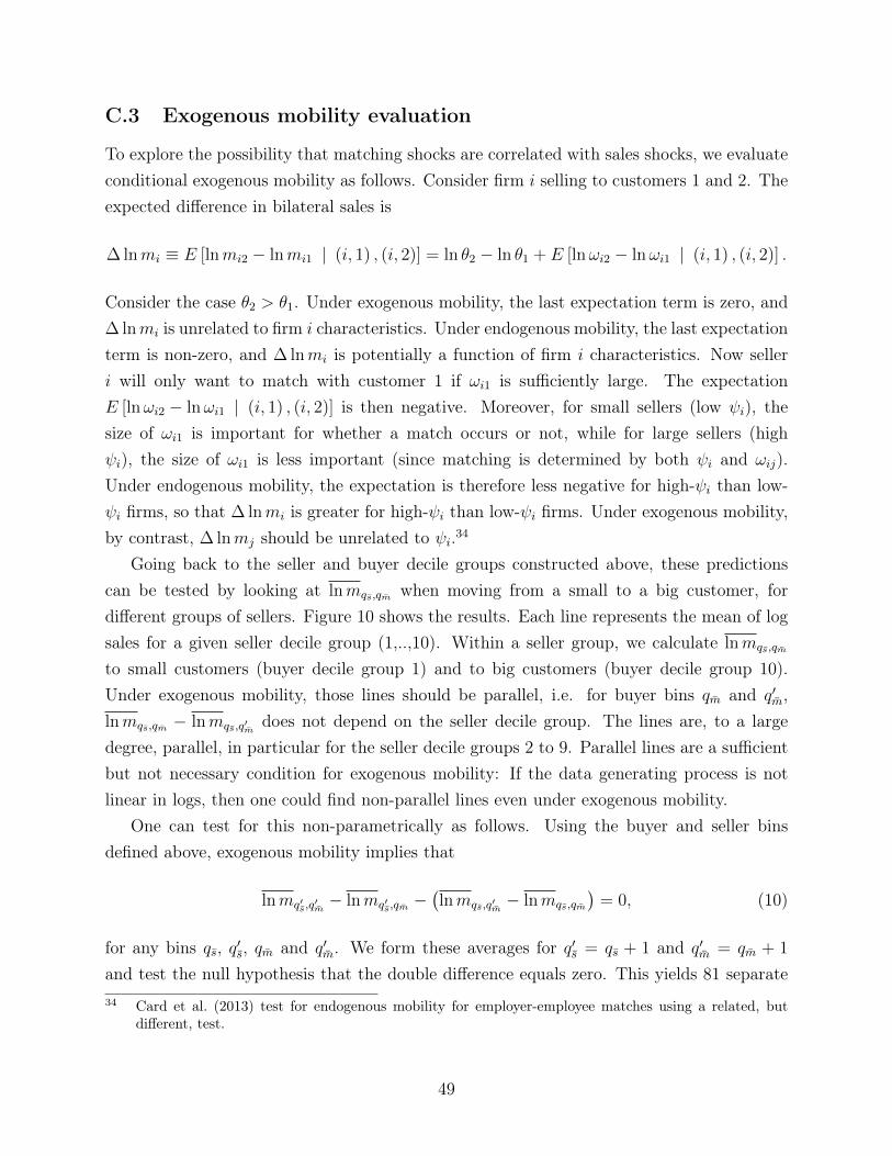
C.3 Exogenous mobility evaluation

To explore the possibility that matching shocks are correlated with sales shocks, we evaluateconditional exogenous mobility as follows. Consider firm i selling to customers 1 and 2. Theexpected difference in bilateral sales is

∆ lnmi ≡ E [lnmi2 − lnmi1 | (i, 1) , (i, 2)] = ln θ2 − ln θ1 + E [lnωi2 − lnωi1 | (i, 1) , (i, 2)] .

Consider the case θ2 > θ1. Under exogenous mobility, the last expectation term is zero, and∆ lnmi is unrelated to firm i characteristics. Under endogenous mobility, the last expectationterm is non-zero, and ∆ lnmi is potentially a function of firm i characteristics. Now selleri will only want to match with customer 1 if ωi1 is sufficiently large. The expectationE [lnωi2 − lnωi1 | (i, 1) , (i, 2)] is then negative. Moreover, for small sellers (low ψi), thesize of ωi1 is important for whether a match occurs or not, while for large sellers (highψi), the size of ωi1 is less important (since matching is determined by both ψi and ωij).Under endogenous mobility, the expectation is therefore less negative for high-ψi than low-ψi firms, so that ∆ lnmi is greater for high-ψi than low-ψi firms. Under exogenous mobility,by contrast, ∆ lnmj should be unrelated to ψi.34

Going back to the seller and buyer decile groups constructed above, these predictionscan be tested by looking at lnmqs,qm when moving from a small to a big customer, fordifferent groups of sellers. Figure 10 shows the results. Each line represents the mean of logsales for a given seller decile group (1,..,10). Within a seller group, we calculate lnmqs,qm

to small customers (buyer decile group 1) and to big customers (buyer decile group 10).Under exogenous mobility, those lines should be parallel, i.e. for buyer bins qm and q′m,lnmqs,qm − lnmqs,q′m

does not depend on the seller decile group. The lines are, to a largedegree, parallel, in particular for the seller decile groups 2 to 9. Parallel lines are a sufficientbut not necessary condition for exogenous mobility: If the data generating process is notlinear in logs, then one could find non-parallel lines even under exogenous mobility.

One can test for this non-parametrically as follows. Using the buyer and seller binsdefined above, exogenous mobility implies that

lnmq′s,q′m− lnmq′s,qm

−(lnmqs,q′m

− lnmqs,qm

)= 0, (10)

for any bins qs, q′s, qm and q′m. We form these averages for q′s = qs + 1 and q′m = qm + 1

and test the null hypothesis that the double difference equals zero. This yields 81 separate34 Card et al. (2013) test for endogenous mobility for employer-employee matches using a related, but

different, test.

49

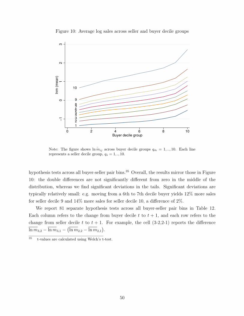
Figure 10: Average log sales across seller and buyer decile groups

1

2345678

9

10

−1

01

23

lnm

(m

ean)

0 2 4 6 8 10Buyer decile group

Note: The figure shows ¯lnmij across buyer decile groups qm = 1, .., 10. Each linerepresents a seller decile group, qs = 1, ., 10.

hypothesis tests across all buyer-seller pair bins.35 Overall, the results mirror those in Figure10: the double differences are not significantly different from zero in the middle of thedistribution, whereas we find significant deviations in the tails. Significant deviations aretypically relatively small: e.g. moving from a 6th to 7th decile buyer yields 12% more salesfor seller decile 9 and 14% more sales for seller decile 10, a difference of 2%.

We report 81 separate hypothesis tests across all buyer-seller pair bins in Table 12.Each column refers to the change from buyer decile t to t + 1, and each row refers to thechange from seller decile t to t + 1. For example, the cell (3-2,2-1) reports the differencelnm3,2 − lnm3,1 −

(lnm2,2 − lnm2,1

).

35 t-values are calculated using Welch’s t-test.

50

Table 12: Exogenous mobility test

Buyer decile2-1 3-2 4-3 5-4 6-5 7-6 8-7 9-8 10-9

Seller decile

2-1 0.01∗ 0.02∗ 0.02∗ 0.03∗ 0.02∗ 0.01 0.01∗ 0.01 -0.04∗

3-2 0.04∗ 0.01∗ 0.01 0.00 0.00 0.01∗ 0.00 0.01 0.02∗

4-3 0.01 0.01∗ 0.02∗ 0.00 0.01 0.00 0.01 0.00 0.03∗

5-4 0.00 -0.01 0.00 0.01∗ 0.00 0.00 0.00 0.00 0.08∗

6-5 0.02∗ 0.02∗ 0.01 0.00 0.01 0.01 0.02∗ 0.00 0.02∗

7-6 0.04∗ 0.02∗ 0.02∗ 0.01∗ 0.01∗ 0.01 0.01 0.03∗ 0.008-7 0.00 0.01∗ 0.00 0.00 0.03∗ -0.01 0.00 -0.01 0.019-8 -0.01 0.02∗ 0.02∗ 0.01 -0.01 0.02∗ 0.01 0.05∗ 0.08∗

10-9 0.03∗ 0.04∗ 0.01 0.02∗ 0.02∗ 0.02∗ 0.02∗ 0.04∗ 0.19∗

Note: The table shows the double difference from equation (10) in the main text. Significance: * <5%, ** < 1%, *** <0.1%. t values are based on Welsh’s t-test.

D Theory Appendix

D.1 Variance decomposition

D.1.1 Identities

We decompose bilateral sales mij into i, j and ij components:

mijdef= Gψiθjωij (11)

where G is a mean across all ij, and without loss of generality, ψi, θj and ωij are definedrelative to that mean. Summing over all customers j of seller i, j ∈ Ci, on both sides:

Sneti

def=∑j∈Ci

mij =∑j∈Ci

Gψiθjωij

= Gψi∑j∈Ci

θjωij (12)

51

where Sneti is the total network sales of i to all its customers j. Total sales of i can beexpressed as an identity:

Si = Sneti

SiSneti

⇒ lnSi = lnSneti + ln βi

where βidef= Si

Sneti≥ 1. Next, we can further decompose the j-specific term in eq.(12) into

components that are observable in the data:

∑j∈Ci

θjωij = nci θiωi1

nci

∑j

θjθi

ωijωi

where nci is the number of business customers j of firm i, and we choose θidef=(∏

j θj

) 1nci

and ωidef=(∏

j ωij

) 1nci to be geometric means of ωij and θj respectively for each i. Taking

logs on both sides:

ln

(∑j∈Ci

θjωij

)= lnnci + ln θi + ln ωi + ln

(1

nci

∑j∈Ci

θjθi

ωijωi

)(13)

= lnnci +1

nci

∑j∈Ci

ln θj +1

nci

∑j∈Ci

lnωij + ln

(1

nci

∑j∈Ci

θjθi

ωijωi

)︸ ︷︷ ︸

def= ln Ωc

i

(14)

Combining all the above leads to the decomposition of sales for every i:

lnSi = lnSneti + ln βi

= lnG+ lnψi + lnnci + ln θi + ln ωi + ln Ωci + ln βi (15)

The residual term ln ωi is obtained from the 2-way FE OLS regression, and by the prop-erties of OLS, ln ωi = 0.

D.1.2 Properties of the Decomposition

Consider first a two component case: lnSnet = lnψ+ln ξ. Then V ar (lnSnet) = V ar (lnψ)+

V ar (ln ξ) + 2Cov(lnψ, ln ξ). When we run an “inverse” regression of components on sales(lnψ = α + β1 lnSnet + ε), OLS estimation implies β1 = Cov(lnSnet,lnψ)

V ar(lnSnet).

52

Note that

Cov(lnSnet, lnψ) = Cov(lnψ + ln ξ, lnψ) (16)

= Cov(lnψ, lnψ) + Cov(ln ξ, lnψ)

= V ar(lnψ) + Cov(ln ξ, lnψ)

where the penultimate equation follows from applying a linear combination of two ran-dom variables. Hence β1 = Cov(lnSnet,lnψ)

V ar(lnSnet)= V ar(lnψ)

V ar(lnSnet)+ Cov(ln ξ,lnψ)

V ar(lnSnet). Similarly for β2 =

Cov(lnSnet,ln ξ)V ar(lnSnet)

= V ar(ln ξ)V ar(lnSnet)

+ Cov(ln ξ,lnψ)V ar(lnSnet)

. Combining both:

β1 + β2 =1

V ar(lnSnet)(V ar(lnψ) + V ar(ln ξ) + 2Cov(ln ξ, lnψ)) = 1 (17)

From eq.(16), we see that these covariances are attributed equally to each component. I.e.the OLS coefficient thus captures the share of total variance in lnSnet explained by the vari-ance in lnψ plus any covariances across components.

The general case for the sum of K ≥ 2 general random variables X =∑K

k=1 Xk is a straight-forward extension, so that

K∑k=1

βk =1

V ar(X)

(∑k

V ar(Xk) +∑i 6=k

Cov(Xi, Xk)

)= 1

Since we perform an exact decomposition (from the identities above), the sum of thevariance shares sum to one, explaining all of the variance in X. Each OLS coefficient for Xk

is equivalent to the share of the variance explained in X.

D.2 Seller Fixed Effect And Average Market Share

This section shows the relationship between seller fixed effects and average market shares.Sales from i to j is mij = eGψiθjωij. Therefore network purchases can be written as

Mnetj = eGθj

∑i∈Sj ψiωij. Rearranging, we get

θj =Mnet

j

eG∑

i∈Sj ψiωij. (18)

53

Seller i’s market share in j’s network purchases is

mij

Mnetj

=eGψiθjωijMnet

j

.

The average of log market shares (i.e., the log of the geometric mean) across i’s customers is

lnMktShi =1

nci

∑j∈Ci

lnmij

Mnetj

=1

nci

∑j∈Ci

lneGψiθjωijMnet

j

= G+ lnψi +1

nci

(∑j∈Ci

lnθjωijMnet

j

).

Substituting θj with equation (18) above, we obtain

lnMktShi = lnψi +1

nci

(∑j∈Ci

lnωij∑

i′∈Sj ψi′ωi′j

)

= lnψi −1

nci

∑j∈Ci

ln τj

where τj ≡∑

i′∈Sj ψi′ωi′j and we used the fact that∑

j∈Ci lnωij = 0 by the properties ofOLS.

D.3 Existence and Uniqueness

We prove existence and uniqueness by showing that the fixed network equilibrium belongsto the class of models analyzed by Allen et al. (2016). They consider the following systemof equations:

K∏h=1

(xhi)γkh = cki +

N∑j=1

Kkij

K∏h=1

(xhj)βkh ,

where i, j ∈ 1, .., N are firms/sectors, xhi is the type h equilibrium variable, cki is a constantand Kk

ij are exogenous linkages between i and j. With K = 1 this reduces to

xγi = ci +N∑j=1

Kijxβj . (19)

54

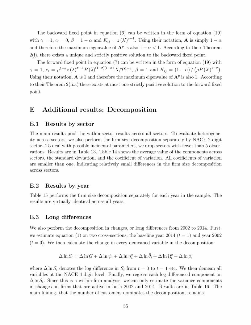
The backward fixed point in equation (6) can be written in the form of equation (19)with γ = 1, ci = 0, β = 1− α and Kij = z (λ′)σ−1. Using their notation, A is simply 1− αand therefore the maximum eigenvalue of Ap is also 1− α < 1. According to their Theorem2(i), there exists a unique and strictly positive solution to the backward fixed point.

The forward fixed point in equation (7) can be written in the form of equation (19) withγ = 1, ci = µ1−σz (λ)σ−1 P (λ)(1−σ)(1−α)X/P1−σ, β = 1 and Kij = (1− α) /

(µP (λ′)1−σ).

Using their notation, A is 1 and therefore the maximum eigenvalue of Ap is also 1. Accordingto their Theorem 2(ii.a) there exists at most one strictly positive solution to the forward fixedpoint.

E Additional results: Decomposition

E.1 Results by sector

The main results pool the within-sector results across all sectors. To evaluate heterogene-ity across sectors, we also perform the firm size decomposition separately by NACE 2-digitsector. To deal with possible incidental parameters, we drop sectors with fewer than 5 obser-vations. Results are in Table 13. Table 14 shows the average value of the components acrosssectors, the standard deviation, and the coefficient of variation. All coefficients of variationare smaller than one, indicating relatively small differences in the firm size decompositionacross sectors.

E.2 Results by year

Table 15 performs the firm size decomposition separately for each year in the sample. Theresults are virtually identical across all years.

E.3 Long differences

We also perform the decomposition in changes, or long differences from 2002 to 2014. First,we estimate equation (1) on two cross-sections, the baseline year 2014 (t = 1) and year 2002(t = 0). We then calculate the change in every demeaned variable in the decomposition:

∆ lnSi = ∆ lnG+ ∆ lnψi + ∆ lnnci + ∆ ln θi + ∆ ln Ωci + ∆ ln βi

where ∆ lnSi denotes the log difference in Si from t = 0 to t = 1 etc. We then demean allvariables at the NACE 4-digit level. Finally, we regress each log-differenced component on∆ lnSi. Since this is a within-firm analysis, we can only estimate the variance componentsin changes on firms that are active in both 2002 and 2014. Results are in Table 16. Themain finding, that the number of customers dominates the decomposition, remains.

55

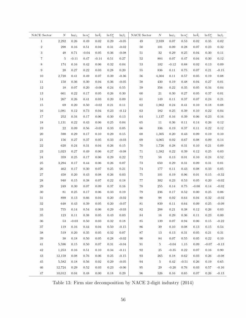
NACE Sector N lnψi lnnci ln θi ln Ωc

i lnβi NACE Sector N lnψi lnnci ln θi ln Ωc

i lnβi

1 2,292 0.26 0.49 0.02 0.29 -0.05 49 2,939 0.07 0.53 0.02 0.35 0.02

2 298 0.16 0.51 0.04 0.31 -0.02 50 101 0.09 0.28 0.07 0.23 0.32

3 48 0.71 -0.04 0.05 0.36 -0.08 51 32 0.29 0.25 0.04 0.30 0.11

7 5 -0.11 0.47 -0.14 0.51 0.27 52 884 0.07 0.47 0.04 0.30 0.12

8 174 0.16 0.42 0.06 0.32 0.04 53 102 -0.12 0.88 0.02 0.13 0.09

9 20 0.27 0.22 0.03 0.28 0.20 55 836 0.11 0.75 0.07 0.21 -0.15

10 2,720 0.41 0.49 0.07 0.39 -0.36 56 4,304 0.11 0.57 0.05 0.19 0.08

11 150 0.36 0.30 0.04 0.36 -0.05 58 430 0.19 0.48 0.04 0.27 0.01

12 18 0.07 0.20 -0.06 0.24 0.55 59 356 0.22 0.35 0.05 0.34 0.04

13 661 0.22 0.17 0.05 0.26 0.30 60 21 0.30 0.27 0.05 0.37 0.01

14 267 0.26 0.41 0.03 0.20 0.09 61 149 0.11 0.37 0.07 0.24 0.21

15 69 0.20 0.50 -0.02 0.21 0.11 62 1,962 0.24 0.41 0.10 0.18 0.08

16 1,081 0.12 0.73 0.04 0.23 -0.12 63 182 0.25 0.39 0.10 0.22 0.04

17 252 0.34 0.17 0.06 0.30 0.13 64 1,137 0.16 0.39 0.06 0.23 0.16

18 1,131 0.22 0.43 0.06 0.25 0.04 65 11 0.36 0.11 0.14 0.26 0.12

19 22 0.09 0.56 -0.03 0.33 0.05 66 336 0.19 0.37 0.11 0.22 0.12

20 590 0.29 0.17 0.10 0.29 0.15 68 1,305 0.20 0.43 0.09 0.19 0.10

21 156 0.27 0.37 0.05 0.33 -0.03 69 4,065 0.02 0.67 0.08 0.09 0.14

22 620 0.24 0.31 0.04 0.26 0.15 70 1,726 0.28 0.31 0.10 0.21 0.09

23 1,023 0.27 0.49 0.06 0.27 -0.08 71 1,382 0.22 0.39 0.12 0.25 0.03

24 359 0.25 0.17 0.06 0.29 0.22 72 58 0.13 0.01 0.10 0.24 0.52

25 3,294 0.17 0.44 0.06 0.26 0.07 73 650 0.29 0.31 0.09 0.31 0.01

26 462 0.17 0.30 0.07 0.25 0.21 74 177 0.11 0.43 0.08 0.33 0.05

27 458 0.20 0.43 0.08 0.26 0.03 75 101 0.19 0.96 0.01 0.15 -0.32

28 940 0.15 0.38 0.07 0.22 0.18 77 302 0.23 0.53 0.05 0.20 -0.02

29 249 0.30 0.07 0.09 0.37 0.16 78 255 0.14 0.75 -0.00 0.14 -0.02

30 81 0.25 0.17 0.06 0.33 0.19 79 236 0.17 0.52 0.00 0.25 0.06

31 899 0.13 0.66 0.04 0.20 -0.02 80 98 0.02 0.64 0.04 0.32 -0.02

32 648 0.43 0.39 0.05 0.20 -0.07 81 839 0.11 0.64 0.09 0.25 -0.09

33 755 0.14 0.54 0.06 0.29 -0.03 82 288 0.21 0.38 0.12 0.26 0.03

35 123 0.11 0.38 0.05 0.43 0.03 84 16 0.29 0.36 0.11 0.23 0.00

36 53 -0.03 0.50 0.03 0.32 0.18 85 139 0.07 0.94 0.06 0.15 -0.22

37 119 0.16 0.44 0.04 0.50 -0.15 86 39 0.10 0.08 0.13 0.15 0.54

38 519 0.20 0.35 0.05 0.32 0.07 87 13 0.13 0.31 0.05 0.21 0.31

39 38 0.18 0.50 0.05 0.28 -0.02 90 84 0.07 0.55 0.05 0.22 0.10

41 5,596 0.15 0.50 0.07 0.31 -0.04 91 5 -0.04 1.15 0.09 -0.07 -0.13

42 1,253 0.16 0.51 0.10 0.34 -0.11 92 25 -0.35 0.22 0.07 0.16 0.90

43 12,159 0.08 0.76 0.06 0.25 -0.15 93 265 0.18 0.62 0.03 0.26 -0.08

45 5,582 0.18 0.56 0.02 0.29 -0.05 94 5 0.42 -0.51 0.26 0.19 0.65

46 12,724 0.29 0.52 0.03 0.23 -0.06 95 29 -0.20 0.76 0.03 0.57 -0.16

47 10,012 0.04 0.48 0.00 0.18 0.29 96 526 0.16 0.65 0.07 0.26 -0.13

Table 13: Firm size decomposition by NACE 2-digit industry (2014)

56

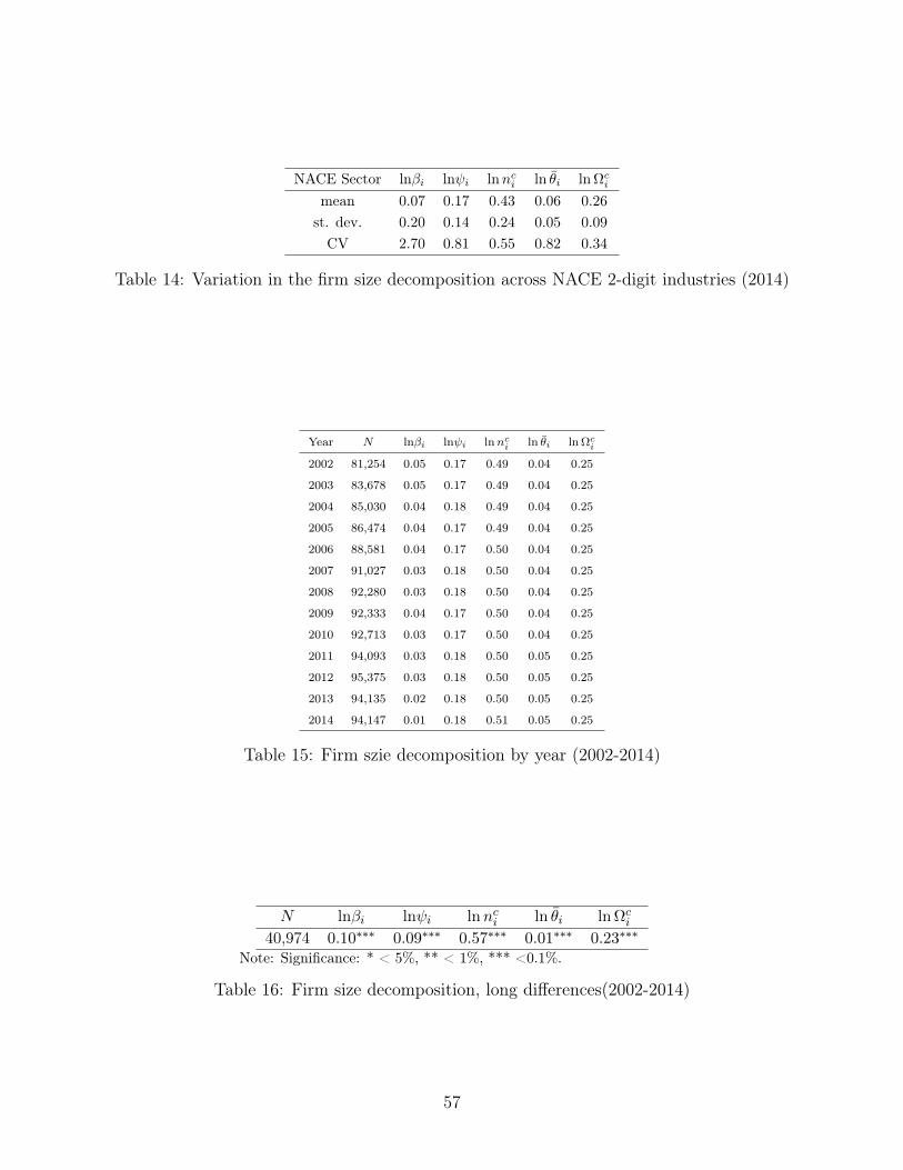
NACE Sector lnβi lnψi lnnci ln θi ln Ωcimean 0.07 0.17 0.43 0.06 0.26st. dev. 0.20 0.14 0.24 0.05 0.09CV 2.70 0.81 0.55 0.82 0.34

Table 14: Variation in the firm size decomposition across NACE 2-digit industries (2014)

Year N lnβi lnψi lnnci ln θi ln Ωc

i

2002 81,254 0.05 0.17 0.49 0.04 0.25

2003 83,678 0.05 0.17 0.49 0.04 0.25

2004 85,030 0.04 0.18 0.49 0.04 0.25

2005 86,474 0.04 0.17 0.49 0.04 0.25

2006 88,581 0.04 0.17 0.50 0.04 0.25

2007 91,027 0.03 0.18 0.50 0.04 0.25

2008 92,280 0.03 0.18 0.50 0.04 0.25

2009 92,333 0.04 0.17 0.50 0.04 0.25

2010 92,713 0.03 0.17 0.50 0.04 0.25

2011 94,093 0.03 0.18 0.50 0.05 0.25

2012 95,375 0.03 0.18 0.50 0.05 0.25

2013 94,135 0.02 0.18 0.50 0.05 0.25

2014 94,147 0.01 0.18 0.51 0.05 0.25

Table 15: Firm szie decomposition by year (2002-2014)

N lnβi lnψi lnnci ln θi ln Ωci

40,974 0.10∗∗∗ 0.09∗∗∗ 0.57∗∗∗ 0.01∗∗∗ 0.23∗∗∗

Note: Significance: * < 5%, ** < 1%, *** <0.1%.

Table 16: Firm size decomposition, long differences(2002-2014)

57

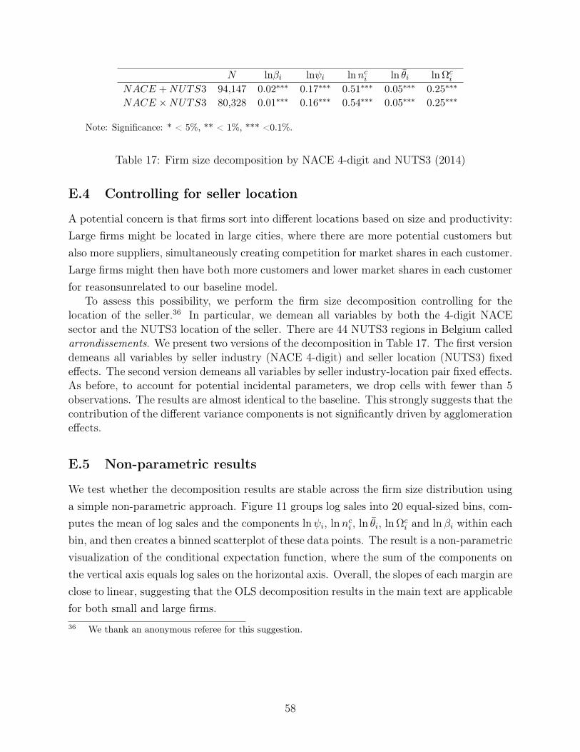
N lnβi lnψi lnnci ln θi ln Ωci

NACE +NUTS3 94,147 0.02∗∗∗ 0.17∗∗∗ 0.51∗∗∗ 0.05∗∗∗ 0.25∗∗∗

NACE ×NUTS3 80,328 0.01∗∗∗ 0.16∗∗∗ 0.54∗∗∗ 0.05∗∗∗ 0.25∗∗∗

Note: Significance: * < 5%, ** < 1%, *** <0.1%.

Table 17: Firm size decomposition by NACE 4-digit and NUTS3 (2014)

E.4 Controlling for seller location

A potential concern is that firms sort into different locations based on size and productivity:Large firms might be located in large cities, where there are more potential customers butalso more suppliers, simultaneously creating competition for market shares in each customer.Large firms might then have both more customers and lower market shares in each customerfor reasonsunrelated to our baseline model.

To assess this possibility, we perform the firm size decomposition controlling for thelocation of the seller.36 In particular, we demean all variables by both the 4-digit NACEsector and the NUTS3 location of the seller. There are 44 NUTS3 regions in Belgium calledarrondissements. We present two versions of the decomposition in Table 17. The first versiondemeans all variables by seller industry (NACE 4-digit) and seller location (NUTS3) fixedeffects. The second version demeans all variables by seller industry-location pair fixed effects.As before, to account for potential incidental parameters, we drop cells with fewer than 5observations. The results are almost identical to the baseline. This strongly suggests that thecontribution of the different variance components is not significantly driven by agglomerationeffects.

E.5 Non-parametric results

We test whether the decomposition results are stable across the firm size distribution usinga simple non-parametric approach. Figure 11 groups log sales into 20 equal-sized bins, com-putes the mean of log sales and the components lnψi, lnnci , ln θi, ln Ωc

i and ln βi within eachbin, and then creates a binned scatterplot of these data points. The result is a non-parametricvisualization of the conditional expectation function, where the sum of the components onthe vertical axis equals log sales on the horizontal axis. Overall, the slopes of each margin areclose to linear, suggesting that the OLS decomposition results in the main text are applicablefor both small and large firms.36 We thank an anonymous referee for this suggestion.

58

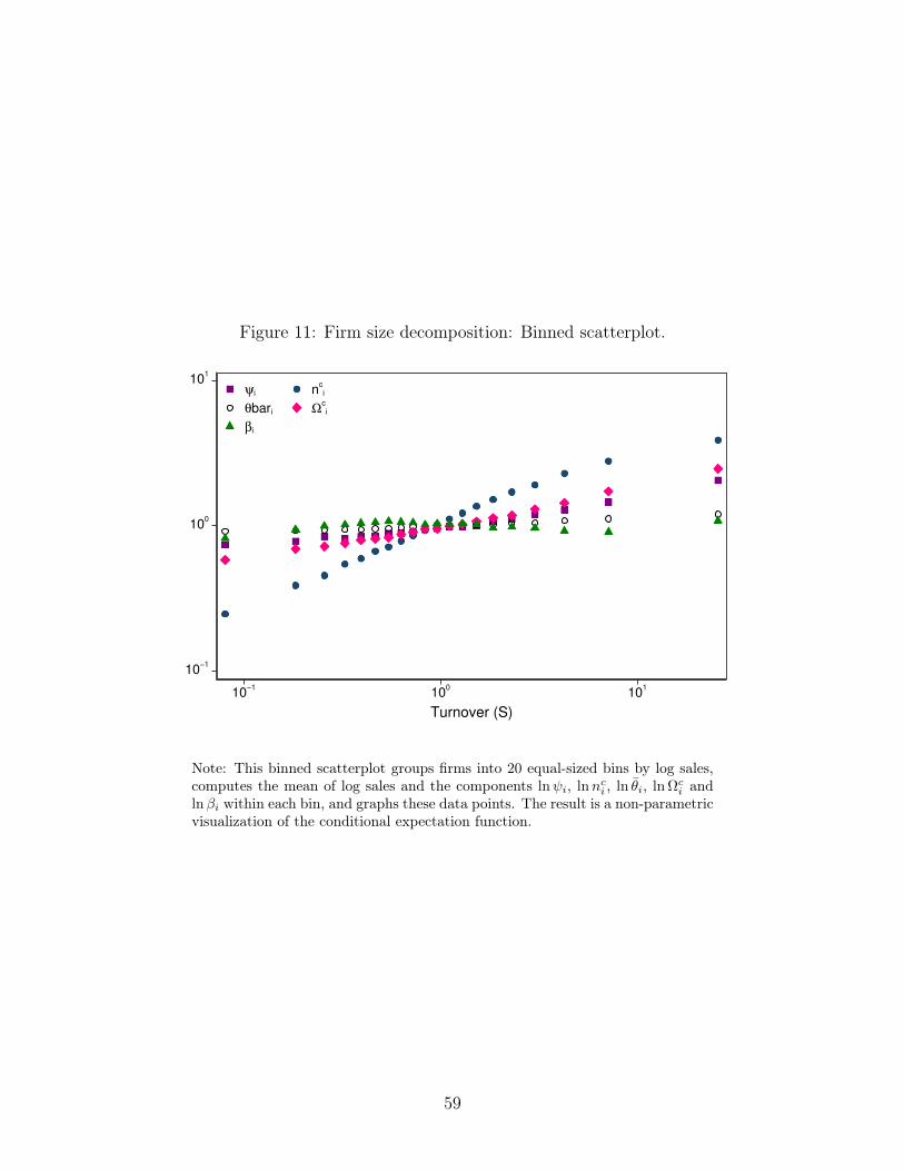
Figure 11: Firm size decomposition: Binned scatterplot.

10−1

100

101

10−1

100

101

Turnover (S)

ψi nci

θbari Ωci

βi

Note: This binned scatterplot groups firms into 20 equal-sized bins by log sales,computes the mean of log sales and the components lnψi, lnnci , ln θi, ln Ωci andlnβi within each bin, and graphs these data points. The result is a non-parametricvisualization of the conditional expectation function.

59

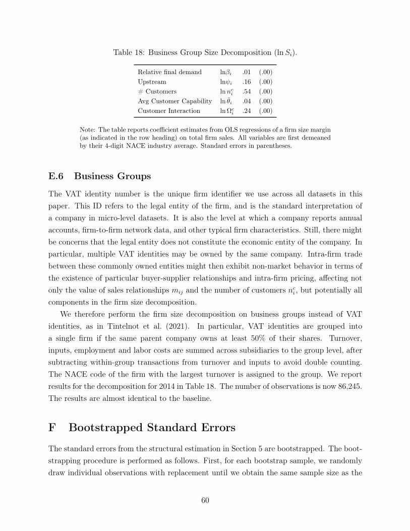
Table 18: Business Group Size Decomposition (lnSi).

Relative final demand lnβi .01 (.00)Upstream lnψi .16 (.00)# Customers lnnci .54 (.00)Avg Customer Capability ln θi .04 (.00)Customer Interaction ln Ωci .24 (.00)

Note: The table reports coefficient estimates from OLS regressions of a firm size margin(as indicated in the row heading) on total firm sales. All variables are first demeanedby their 4-digit NACE industry average. Standard errors in parentheses.

E.6 Business Groups

The VAT identity number is the unique firm identifier we use across all datasets in thispaper. This ID refers to the legal entity of the firm, and is the standard interpretation ofa company in micro-level datasets. It is also the level at which a company reports annualaccounts, firm-to-firm network data, and other typical firm characteristics. Still, there mightbe concerns that the legal entity does not constitute the economic entity of the company. Inparticular, multiple VAT identities may be owned by the same company. Intra-firm tradebetween these commonly owned entities might then exhibit non-market behavior in terms ofthe existence of particular buyer-supplier relationships and intra-firm pricing, affecting notonly the value of sales relationships mij and the number of customers nci , but potentially allcomponents in the firm size decomposition.

We therefore perform the firm size decomposition on business groups instead of VATidentities, as in Tintelnot et al. (2021). In particular, VAT identities are grouped intoa single firm if the same parent company owns at least 50% of their shares. Turnover,inputs, employment and labor costs are summed across subsidiaries to the group level, aftersubtracting within-group transactions from turnover and inputs to avoid double counting.The NACE code of the firm with the largest turnover is assigned to the group. We reportresults for the decomposition for 2014 in Table 18. The number of observations is now 86,245.The results are almost identical to the baseline.

F Bootstrapped Standard Errors

The standard errors from the structural estimation in Section 5 are bootstrapped. The boot-strapping procedure is performed as follows. First, for each bootstrap sample, we randomlydraw individual observations with replacement until we obtain the same sample size as the

60

main dataset. Then, for each bootstrap sample, we create the empirical moments used inthe simulated method of moments estimation. We create 200 bootstrap moments in total.Finally, we estimate the parameters of the model 200 times using the 200 different bootstrapmoments. The standard deviations of the estimated parameters are the standard errorsreported in Table 5.

61