Submitted version June 28, 2002

The Palomar/MSU Nearby Star Spectroscopic Survey IV: The

Luminosity Function in the Solar Neighbourhood and M Dwarf

Kinematics 1

I. Neill Reid

Space Telescope Science Institute, 3700 San Marin Drive, Baltimore, MD 21218

and

Department of Physics and Astronomy, University of Pennsylvania, 209 South 33rd Street,

Philadelphia PA 19104-6396

inr@stsci.edu

John E. Gizis

Department of Physics & Astronomy, University of Delaware

gizis@udel.edu

Suzanne L. Hawley

Astronomy Dept, Box 351580, Univ of Washington, Seattle, WA 98195

slh@pillan.astro.washington.edu

ABSTRACT

We have used new astrometric and spectroscopic observations to refine the

volume-complete sample of M dwarfs defined in previous papers in this series.

With the addition of Hipparcos astrometry, our revised VC2 sample includes 558

main-sequence stars in 448 systems. Analysis of that dataset shows no evidence

for any systematic kinematic bias. Combining those data with an Hipparcos-

based sample of AFGK dwarfs within 25 parsecs of the Sun, we have derived

the Solar Neighbourhood luminosity function, Φ(MV ), for stars with absolute

magnitudes between -1 and +17. Using empirical and semi-empirical mass-MV

relations, we transform Φ(MV ) to the present-day mass function, ψ(M) ( dNdM

).

Depending on the mass-luminosity calibration adopted, ψ(M) can be represented

by either a two-component or three-component power-law. In either case, the

– 2 –

power-law index, α, has a value of ∼ 1.3 at low masses (0.1 < MM�

< 0.7), and

the local mass density of main sequence stars is ∼ 0.031M�pc−3.

We have converted ψ(M) to an estimate of the initial mass function, Ψ(M), by

allowing for stellar evolution, the density law perpendicular to the Plane and the

local mix of stellar populations. The results give α = 1.1 to 1.3 at low masses,

and α = 2.5 to 2.8 at high masses, with the change in slope lying between 0.7

and 1.1M�.

Finally, the (U, W) velocity distributions of both the VC2 sample and the fainter

(MV > 4) stars in the Hipparcos 25-pc sample are well-represented by two-

component Gaussian distributions, with ∼10% of the stars in the higher velocity-

dispersion component. We suggest that the latter component is the thick disk,

and offer a possible explanation for the relatively low velocity dispersions shown

by ultracool dwarfs.

Subject headings: (Galaxy:) solar neighborhood — stars: kinematics — stars:

luminosity function, mass function

1. Introduction

The nearest stars represent an important tool in studies of Galactic structure, since they

provide an opportunity for detailed analysis of constituent members of the various stellar

populations and sub-populations. This holds particularly for M dwarfs, which account for

the overwhelming majority of stars currently present in the Galaxy. With a local density

of ∼ 0.07 pc−3, these stars are ideal tracers of many properties of the Galactic disk. Until

recently, the main limitation in such analyses was the lack of basic observational data, such

as spectral types or radial velocities. Our main goal in undertaking the Palomar/Michigan

State University (PMSU) survey (Reid, Hawley & Gizis, 1995, PMSU1; Hawley, Gizis &

Reid, 1996, PMSU2; Hawley, Gizis & Reid, 1997), was to remedy this defect by compiling

moderate resolution spectroscopy for all M dwarfs in the preliminary version of the third

Catalogue of Nearby Stars (Gliese & Jahreiß, 1991; pCNS3). We obtained observation of

over 2000 candidate M dwarfs, omitting only unresolved binary companions. Calculating

distances by combining spectroscopic parallaxes with the then-available trigonometric data,

we defined MV -dependent distance limits which isolate a volume-complete sample, and used

1Based partly on observations made at the 60-inch telescope at Palomar Mountain which is jointly owned

by the California Institute of Technology and the Carnegie Institution of Washington

– 3 –

that sample to derive estimates of the luminosity function and the velocity distribution of low

mass stars (PMSU1), in addition to studying the range of chromospheric activity (PMSU2).

Since the completion of our initial analysis, two major new datasets have become avail-

able. First, the Hipparcos catalogue has been published (ESA, 1997), including milliarcsecond-

accuracy astrometry for over 110,000 stars brighter than 13th magnitude. Almost two-thirds

of the stars in the pCNS3 have observations by Hipparcos. Second, as a follow-up to PMSU,

we obtained echelle spectroscopy of many of the brighter M dwarfs in the pCNS3, includ-

ing all of the stars in the volume-complete sample defined in PMSU1. Those data are now

fully analysed, and presented by Gizis, Reid & Hawley (2002; PMSU3). The high-resolution

observations provide significantly more accurate radial velocities, besides more sensitive mea-

surement of chromospheric activity.

Both of these new datasets have potential importance for the results of the analysis

presented in PMSU1. Revising the distances of a substantial number of stars affects both

the composition of the volume-complete sample and the derived tangential motions, while

the new radial velocity determinations affect the space motion determinations. We have

therefore re-analysed the PMSU dataset, incorporating the new observational data. Section

2 describes the definition of the revised volume-complete sample; section 3 considers the

effect on the luminosity function; section 4 rederives the mass function for nearby stars,

combining our data with an Hipparcos 25-parsec sample of earlier-type main-sequence stars;

and section 5 re-analyses the kinematics. The main results are summarised and discussed in

section 6.

2. A volume-complete sample of Solar Neighbourhood M dwarfs

In PMSU1, we used the available trigonometric and photometric parallax information,

together with our own distance estimates based on the (MV , TiO5) calibration, to construct

a volume-complete (VC) subset of the M dwarfs in the pCNS3. Over 2300 pCNS3 stars have

Hipparcos astrometry, but, with incomplete sampling between V=8 and the Hipparcos limit

of V=13, that dataset includes only 712 M dwarfs from PMSU1 and PMSU2. Coverage is

better amongst the brighter stars in the PMSU1 VC subset, however, with data for 330 of

the 499 systems.

Figure 1 compares pre- and post-Hipparcos distance measurements for PMSU stars;

there is a systematic shift towards higher distances (parallaxes tend to be overestimated,

hence the Lutz-Kelker bias), and a significant number of M dwarfs move beyond the 25

parsec boundary of the pCNS3. Seventy-one of the 499 systems in the VC sample have revised

– 4 –

distances which place the stars beyond the completeness limits adopted for the appropriate

absolute magnitude. We have therefore re-analysed the pCNS3 dataset, augmented by new

observations, and derive a revised volume-complete sample of M dwarfs, (VC2).

2.1. Re-defining the sample

We have used the techniques described in PMSU1 to analyse the post-Hipparcos pCNS3

dataset, re-deriving the appropriate distance limits as a function of absolute magnitude. As

before, we limit analysis to the 1684 M dwarf systems in the northern sample, δ > −30◦,

and set absolute magnitude limits 8 ≤ MV ≤ 16. Figure 2 provides the justification for

our choice of distance limits, plotting the run of density (ρsys, number of systems per unit

volume) with increasing distance; the distance limits, dlim, are set where ρsys flattens, before

the downturn due to incompleteness. Applying Schmidt’s (1968) V/Vmax estimator to the

same issue gives identical results.

As Table 1 shows, the revised distance limits match those derived in PMSU1, with

the exception of the MV =9.5 bin, where dlim decreases by 10%. A total of 545 stars in

435 systems, including 300 with Hipparcos data, meet these distance criteria. This dataset

includes additional companions identified by Reid & Gizis (1997, RG97), Delfosse et al.

(1999) and Beuzit et al. (2001). Only 16 systems lack PMSU3 echelle observations, and the

majority (381 systems) have distances derived from trigonometric parallaxes. The relevant

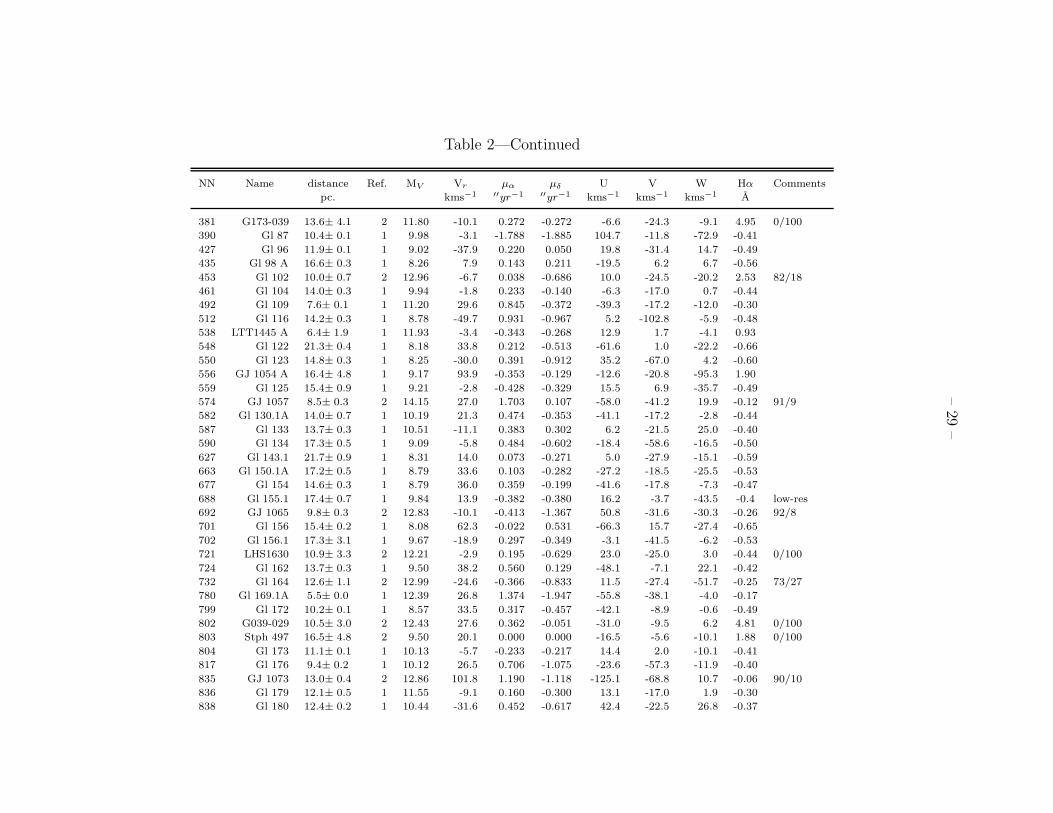
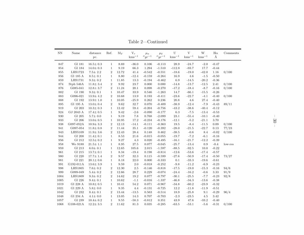
data for each stellar system are listed in Table 2, where we also give the proper motions and

space velocities.

Besides providing improved distance estimates for stars already known to lie within

the immediate Solar Neighbourhood, Hipparcos also identified a number of previously-

unrecognised nearby stars. The full catalogue lists 78 stars which are not in the pCNS3,

but have πH > 45 milliarcseconds (mas) or r < 22 parsecs. Of these, 23 have formal ab-

solute magnitude values in the range 8 ≤ MV ≤ 16. Ten of the latter subset, however,

have spectral types which are clearly inconsistent with the inferred absolute magnitude; for

example, HIP 21000, or BD+4:701A, has πH = 84.8 mas and an inferred MV = 9.5, but

spectral type F8. All ten are in binary systems, and the companion has influenced the as-

trometric results listed in the Hipparcos catalogue. This is a well known problem, which can

be rectified through more sophisticated analysis; thus, Fabricius & Makarov (2000) derive

πH ′ = 4.2 mas for HIP 21000.

The remaining 13 stars in the supplementary sample are all confirmed M dwarfs. The

parallax measurements for both Vyssotsky 130 (a double star) and HD 218422 have substan-

– 5 –

tial uncertainties. For the present, we retain both stars in the sample, increasing the revised

VC2 sample to 558 main-sequence stars2 in 448 systems. Relevant data for the additional

stars are listed in Table 3. With the exception of LHS 1234 (Weis, 1996), prior observations

are scarce, and most lack radial velocity data. For those stars, the space motions listed in

Table 3 are computed for Vr = 0 km s−1 .

2.2. Biases and completeness

A reliable determination of the properties of the local Galactic Disk demands an unbi-

ased, representative stellar dataset. It is to that end that we constructed the VC2 sample

described in the previous section. However, while the ρ(d) and VVmax

(d) measurements show

that the sample as a whole is broadly consistent with our requirements, subtle biases may

remain, particularly since the stars are drawn primarily from a pre-existing catalogue (the

pCNS3) rather than an unbiased all-sky survey. On the positive side, our VC2 sample has

the advantage that trigonometric parallax measurements are the dominant contributor to

distance estimates for 90% of the systems. This is in contrast to the original PMSU1 VC

sample, where 40% of the stars lacked accurate astrometry.

Two potential sources of bias are proximity to the Galactic Plane, where crowding

might be a problem leading to omission of nearby stars; and proper motion-based selection,

which could bias against nearby stars with low space motions. Considering the former issue,

Figure 3 plots the distribution of the VC2 sample on the celestial sphere. Based on the areal

coverage, we expect 15.9% of the sample to lie within ±10◦ of the Galactic Plane; in fact,

69 of the 448 systems (15.4 ± 1.9%) lie within those limits. We conclude that crowding in

the Galactic Plane is not a significant contributor to incompleteness in the VC2 sample3

A greater concern is the potential for kinematic bias. As discussed in PMSU1 and

PMSU2, most stars in the pCNS3 were identified based on their having high proper motion.

Those stars are drawn predominantly from three major proper motion surveys: the Lowell

survey, limited to µ > 0.26′′ yr−1 (Giclas, Burnham & Thomas, 1971); the Luyten Half

Second catalogue (LHS), µ > 0.50′′ yr−1 , (Luyten 1979); and the New Luyten Two-Tenths

Catalogue (NLTT), µ > 0.18′′ yr−1 , (Luyten, 1980). Those limits correspond to transverse

2There are an additional four white dwarf and three brown dwarf companions.

3We note that there is a statistically significant bias against low-latitude systems if we consider low

luminosity stars in the full pCNS3: of the 395 stars north of −30◦ with with MV > 13, only 41, or 10.4%±

1.8%, lie within 10◦ of the plane. The distance and MV limits imposed in defining the VC2 sample have

eliminated this potential source of bias.

– 6 –

velocities of, respectively, 24.6 km s−1 , 47.4 km s−1 and 17.1 km s−1 at 20 parsecs. Of

the three surveys, the last has received least attention. While Weis (1986, 1987, 1988) has

obtained (B)VRI photometry for many of the brighter (mr ≤ 13.5) red stars in the NLTT, it

is only recently that systematic attempts have been made to identify nearby stars amongst

the fainter members of that catalogue (Reid & Cruz, 2001; Salim & Gould, 2002) Thus, there

is a clear potential for bias against stars with low tangential motions in both the pCNS3 and

the VC2 sample.

We can test for kinematic bias by comparing the proper motions and transverse motions

of the full VC2 sample against similar data for the subset of stars which are included in the

objective prism surveys (Vyssotsky, 1956; Upgren et al., 1972). Since the latter stars were

identified based on spectral type, that sample should be free of any kinematic selection

effects. Two hundred and nine of the 448 systems in the VC2 sample are in the Vyssotsky

catalogue, while the Upgren et al. survey contributes four systems.

Most of the spectroscopically-selected stars are early-type M dwarfs, and those stars lie

predominantly at larger distances in the VC2 sample. This is illustrated in the upper panels

of Figure 4. Since the average distance of the spectroscopic subset is higher than the full

sample, we must compare the tangential velocity distributions, rather than the proper motion

distributions. That comparison is shown in the lower panels of Figure 4, where the dotted

line in the right-hand panel marks the fractional contribution of the spectroscopic subset to

the full sample. If there were a significant bias against stars with low transverse motions, we

would expect the proportion of spectroscopically-selected stars to rise with decreasing Vtan.

The data show little evidence for that effect. Dividing the distribution into two subsets, with

Vtan ≤ 20 kms−1 and Vtan > 20 kms−1, the ratiosNprism

Ntotare 44.0 ± 7.4% and 48.6 ± 4.7%,

respectively.

Our tests therefore reveal no evidence for significant bias in the VC2 sample either

against stars lying within 10 degrees of the Galactic Plane, or against stars with low tan-

gential motions. On that basis, we conclude that the VC2 sample provides a reliable dataset

for examining the space density and kinematics of the local Galactic Disk population.

3. The Luminosity Function

3.1. The Luminosity Function

We next consider how the revised distances obtained by Hipparcos affect the nearby-star

luminosity function, Φ(MV ). We also take this opportunity to redetermine Φ(MV ) for earlier-

type (BAFGK) main-sequence stars in the Solar Neighbourhood, and to identify lower-mass

– 7 –

companions to those stars which should be added to the PMSU M dwarf statistics. Despite

the availability of Hipparcos data for more than half a decade, many recent luminosity-

function analyses are still based on the statistics compiled by Wielen, Jahreiß & Kruger

(1983) from the second Catalogue of Nearby Stars (Gliese, 1969; CNS2) and its supplement

(Gliese & Jahreiß, 1979). An exception is the sample discussed by Kroupa, 2001. Clearly,

the systematics evident in Figure 1 have a significant influence on our estimate of the local

density of main-sequence stars.

The Hipparcos catalogue has a formal completeness limit of

V = 7.9 + 1.1sin|b|

so the 25-parsec sample is effectively complete over the whole sky for MV ≤ 5.9. However,

since the mission involved pointed observations of pre-selected targets, the survey includes a

high proportion of stars known or suspected of being in the immediate Solar Neighbourhood.

Indeed, Jahreiß and Wielen (1997) argue that the Hipparcos catalogue is essentially complete

to MV = 8.5 for stars within 25 parsecs of the Sun, providing a useful complement to the

8 < MV < 16 VC2 sample.

We have identified 831 Hipparcos stars with πH ≥ 40 milliarcseconds (mas) and MV ≤

8.0. Three issues need to be addressed before deriving a luminosity function from this

dataset: the evolutionary status of the individual stars; binarity and multiplicity; and the

local intermix of stellar populations. The first and last considerations are illustrated in

Figure 5, which plots the (MV , (B-V)) colour-magnitude diagram for all 1477 stars in the

Hipparcos catalogue with πH ≥ 40 mas. Evolved stars clearly make a significant contribution

at brighter magnitudes, and we have excluded them by eliminating stars which meet the

following criteria,

MV < 7.14(B − V ) − 1.0, and MV < 5.0

This removes 41 stars from the sample.

Figure 5 includes a number of stars lying well below the disk main sequence. Most are

fainter than MV =8.0 and are either white dwarfs, stars with substantial uncertainties in the

measured parallax, or stars lacking (B-V) colours. Four stars, however, lie just below the

main sequence with 6 < MV < 8. These are the halo subdwarfs HIP 18915 (HD 25329,

[Fe/H]=-1.6), HIP 57939 (HD 103095, [Fe/H]=-1.4), HIP 67655 (HD 120559, [Fe/H]=-0.94)

and HIP 79537 (HD 145417, [Fe/H]=-1.25). While the statistics are not overwhelming, a

total of four subdwarfs in a sample of ∼ 650 FGK disk dwarfs implies a local number ratio

of ∼ 0.6± 0.3%, a factor of three higher than the density normalisation adopted for the halo

in most Galactic structure analyses. All four stars are excluded from the present analysis.

Finally, we have checked SIMBAD for references to binary and multiple systems amongst

– 8 –

the remaining 786 stars. Thirteen systems have wide companions listed separately in the

Hipparcos database, while a further 213 have unresolved companions at small separations

or wide companions which are not included in the Hipparcos dataset. Where necessary, we

have adjusted the photometry to allow for the contribution from fainter components, most

notably in the case of HIP 66212 (HD 110836), which the uncorrected Hipparcos data place

well above the main sequence. As illustrated in Figure 6, these corrections move a handful

of primary stars to magnitudes fainter than MV =8.0.

Even after applying photometric adjustments, a small number of stars still lie well

above the main sequence in figure 6. Some (e.g. Gl 610) may be unrecognised binaries.

Several, however, are primaries in binary systems (e.g. Gl 795A, GJ 1161A, Gl 118.2A), and

the presence of the known secondary may affect either the photometry or the astrometry.

Others are metal-rich stars (e.g. Gl 614, Gl 848.4 and HD 217107, all known to harbour

extrasolar planets), while still others, lying near the base of the subgiant branch, may be

slightly evolved (e.g. Gl 19, Gl 368). Further spectroscopy and photometry are required to

resolve these issues completely.

We noted above that the Hipparcos dataset is expected to be effectively complete within

25 parsecs for stars with MV < 8.5. We can test this hypothesis using the same techniques

applied to the PMSU M dwarfs in §2. Figure 7 plots the run of density with distance for

systems where the primary has MV = 4.5 ± 0.5.5.5 ± 0.5, 6.5 ± 0.5, and 7.5 ± 0.5. The first

point marks the average density within a sphere, radius 16 parsecs, centred on the Sun;

subsequent point plot the densities within annuli of radii 16 to 18, 18 to 20, 20 to 22 and 22

to 25 parsecs. Given Poisson uncertainties, there is no evidence for a significant decline in

completeness as one approaches the 25-parsec distance limit.

Our final sample includes 764 Hipparcos systems with d < 25 parsecs and MV < 8.0.

A further twelve binaries have primaries with 8 < MV < 9. Four of those stars are already

included in the PMSU sample, while three stars lie beyond 22 parsecs (the PMSU distance

limit appropriate to this absolute magnitude). The remaining five stars are added to the

PMSU sample. We also extend coverage to MV ≥ 16 by adding data for the three systems

currently known with d < 5 parsecs and δ > −30o (GJ 1111, Gl 406 and LHS 292). Table 4

gives final statistics for the combined PMSU and Hipparcos 25-parsec samples, and Figure

8 plots the composite luminosity function, Φ(MV ).

We have compared our results against the luminosity function derived by Wielen, Jahreiß

& Kruger (1983). The space densities derived here are systematically lower than in the earlier

study, reflecting the systematic errors present in pre-Hipparcos distance estimates. Kroupa

(2001) finds similar results in his analysis. Overall, we derive a local number density of

0.106 main sequence stars pc−3, and a density of 0.0725 systems pc−3. With evolved systems

– 9 –

contributing a further 41 systems within 25 parsecs (6.3×10−4 pc−3), the average separation

between systems is ∼ 2.4 parsecs.

3.2. Binarity and Multiplicity

The 764 systems in our Hipparcos 25-parsec upper main-sequence sample include 538

single stars, 204 binaries (including 8 low amplitude spectroscopic binaries from Nidever et

al., 2002), 22 triples and 4 quadruple systems. The resultant multiplicity fraction is only

30.1±2.4%, somewhat lower than the value of 44% derived in the standard reference for this

subject, Duquennoy & Mayor’s (1991, DM91) analysis of observations of solar-type dwarfs.

This discrepancy may reflect poorer observational coverage of the Hipparcos sample. Even

with the addition of the extensive radial velocity data from the Lick/Keck planet-search

survey, summarised by Nidever et al. (2002), 98 stars lack radial velocity measurements,

and we noted in the previous section that a number of stars lie above the main sequence,

suggesting unrecognised binarity.

An alternative possibility is that the multiplicity fraction measured for the 25-parsec

sample is more reliable than the DM91 statistics. The lower binarity might be a consequence

of the larger magnitude range spanned by the present sample, since M dwarfs are known to

have a lower fraction of stellar companions than solar-type stars (Fischer & Marcy, 1992;

RG97). In addition, the improved parallax data lead to a better-defined sampling volume

for the present dataset than for the DM91 dataset. We explore these issues here.

In analysing the multiplicity of solar-type stars, Duquennoy & Mayor’s intention was

to define a volume-limited sample, including systems with spectral types between F7 and

G9, declinations δ > −15 deg and parallaxes exceeding 45 milliarcseconds. However, since

the parallaxes were drawn from the CNS2, they are subject to the systematic errors and

potential biases illustrated in Figure 1. Fortunately, all of the DM91 stars are included in

the Hipparcos catalogue.

Figure 9 compares parallax data listed in the CNS2 against Hipparcos measurements for

the DM91 reference sample. As expected, over 40% of the sample lie beyond the nominal 25-

parsec distance limit, including almost all stars with (B-V)>0.8, most of which are subgiants.

Only 102 systems have πH ≥ 45 milliarcseconds. However, of those 102 systems, 42 are

double or multiple, giving a multiplicity fraction of 41±7%, consistent with the value of 44%

derived for the full dataset in DM91. Observational bias in the DM91 sample is therefore not

likely to be responsible for the discrepancy with respect to the Hipparcos 25-parsec sample.

Even with the extensive temporal coverage and high accuracy provided by the CORAVEL

– 10 –

radial velocity observations, it is likely that a significant number of binary systems remain

unrecognised amongst the DM91 G-dwarf sample. Binary systems with high inclination

and/or long period have low velocity amplitudes, and are therefore more difficult to detect.

Duquennoy & Mayor concluded that their analysis might underestimate the binary fraction

amongst G dwarfs by approximately one-third, implying a true multiplicity close to 60%.

On the other hand, 47 of the 60 “single” stars in the πH ≥ 45 mas DM91 sub-sample are

included in the Lick/Keck planet search program: 46 are classed as having stable radial ve-

locities (σV < 0.1 kms−1); only HIP 98819 (Gl 779) is identified as a confirmed spectroscopic

binary (Nidever et al., 2002).

Based on these results, we take 60% as a likely upper limit for the multiplicity of the

upper main-sequence stars in the Hipparcos 25-parsec sample. Given the relatively sparse

observational scrutiny, we assume that the known secondaries are characteristic of the sample

as a whole, and therefore allow for potential “missing” binary companions by giving double

weight to known binary components in the statistical analysis. Figure 10 shows the resultant

effect on Φ(MV ): the space densities are still systematically lower than the Wielen et al.

(1983) values. The overall space density becomes 0.112 stars pc−3.

4. The Mass Function

4.1. The Mass-Luminosity Relation

The mass-luminosity relation is a key ingredient in transforming the stellar luminosity

function to a mass function. Since we have only B, V data for most of the stars in the

present sample, we require a relation between mass and MV . In general, masses can be

derived only for stars in binary systems (gravitational lensing offers the potential for deriving

accurate masses for single stars, but requires particular source-lens geometries). Henry &

McCarthy (1993) provided the first extensive analysis of lower main-sequence astrometric

binaries. They derive a three-segment fit in the (MV , log(mass)) plane, extending from 2M�

to the hydrogen-burning limit. Together with their mass-MK and mass-Mbol relations, this

calibration has served as the primary reference over the last decade.

Most recent attention has centred on low-mass stars, with the addition of new data

from high-precision HST (Henry et al., 1999) and ground-based astrometry, and from high-

accuracy radial velocity measurements (Delfosse et al., 1999; Segransan et al., 2000). Delfosse

et al. (2000: D00) have used these new observations to derive a revised mass-MV relation

for lower main-sequence stars,

logM = 10−3 × [0.3 + 1.87MV + 7.614M2v − 1.698M3

V + 0.06096M4v ]

– 11 –

As Figure 11 shows, this relation predicts higher masses by 10 to 15% than Henry et al.’s

calibration for 11 < MV < 15.

Delfosse et al. limit their analysis to M dwarfs, and Henry et al’s piecewise mass-MV

relation extends only to 2M�, but the Hipparcos 25-parsec sample includes more massive A-

and B-type stars. We have therefore used the data compiled by Andersen (1991) for eclipsing

binary systems to derive an empirical mass-MV relation covering the upper main-sequence.

That relation is

logM = 0.477 − 0.135Mv + 1.228 × 10−2M2v − 6.734 × 10−4M3

V

and is plotted in Figure 11. We combine that relation with the D00 result, setting the

boundary between the two calibration at MV =10.0, where the agreement is better than 5%.

In addition to these empirical calibrations, Kroupa, Tout & Gilmore (1993, KTG) de-

rived a semi-empirical mass-MV relation. Adopting the Wielen et al. (1983) luminosity

function as a reference, they represent the mass function as a three-component power-law,

and vary the indices to minimise residuals in the mass-MV relation. Figure 11 compares

their derived relation against the empirical results. The KTG calibration, spanning absolute

magnitudes between MV =+2 and +17, matches the D00 relation at low masses, and lies up

to 8% below the empirical relation (i.e. predicts lower masses at a given MV ) for solar-mass

stars.

4.2. The Present-day Mass Function

We have computed present-day mass functions using both the D00 empirical calibration

and the KTG semi-empirical relation, extending both to higher masses using our fit to the

Andersen eclipsing binary dataset. Figure 12 shows the results derived from the empirical

calibration. Defining

ξ(M) =dN

d logMand ψ(M) =

dN

dM

the uppermost panel plots ξ(M) for the Hipparcos 25-parsec and the PMSU samples (i.e.

the dataset used to construct Φ(MV ) in Figure 8). The dotted histogram shows the mass

function derived from single stars and primaries in multiple systems. The middle panel in

Figure 12 plots ξ2B(M), where double weight is given to the Hipparcos 25-parsec secondary

components (i.e. the dataset used to construct Figure 10). Adding the hypothetical as-yet-

undiscovered binaries produces little change in the overall morphology. Integrating the mass

functions, we derive a local mass density of ρMS = 0.0310M�pc−3 from ξ(M) and 0.0338

M�pc−3 when double weight is given to the secondaries in the Hipparcos sample. We note

that white dwarfs contribute a further 0.004 M�pc−3 (RG97).

– 12 –

We have also used the empirical mass-MV relation to re-compute the mass function

derived from the northern (δ ≥ −30 deg) 8-parsec sample. The original sample from RG97

has been updated to take into account Hipparcos parallax data and new stellar companions

(Reid et al., 1999; R99). Chabrier & Baraffe (2000) and Kroupa (2001) have suggested that

this sample provides unreliable statistics, both through the inclusion of stars whose distances

rest on photometric/spectroscopic parallax estimators, and through incompleteness. Neither

objection is valid. As emphasised in R99, 100 of the 104 systems have accurate (ε < 10%)

trigonometric parallax measurements, while only a handful of addition have been identified

since 1997. The most recent is 2MASS J1835379+325954, an M8 dwarf at 5.7 parsecs (Reid

et al., 2002a). As discussed in that paper, the >30% deficit in number density between

the 8-parsec and extrapolated 5-parsec sample (Henry et al., 1997) includes a substantial

contribution from bright (MV < 14) stars, and probably overestimates the shortfall by at

least a factor of two.

The mass function derived from the 8-parsec sample is plotted in the lowermost panel

of Figure 12. Again, the single star/primary mass function is plotted as a dotted histogram.

Below 1 M�, the results are statistically identical to those based on the composite Hipparcos

25-pc./PMSU analysis (i.e., employing a 5-parsec limit at MV > 15). The total mass density

derived by integrating ξ8(M) is 0.0288 M�pc−3, the lower value reflecting the relative scarcity

of G dwarfs within 8 parsecs of the Sun4.

Following Salpeter (1955), it is convenient to represent the mass function as a power-law,

ξ(M) = M−α+1 and ψ(M) = M−α,

where α = 2.35 is the Salpeter slope. The mass functions plotted in Figure 12 are all well

represented by a two-component power-law. Both Hipparcos/PMSU analyses are consistent

with α = 1.35 ± 0.2 for 0.1 < MM�

< 1 and α = 5.2 ± 0.4 for M > 1M�. The steep slope at

masses above 1M� emphasises the fact that ξ(M) is the present-day mass function (Miller

& Scalo, 1979); our calculations take no account of higher mass stars which have evolved

off the main sequence over the lifetime of the Galactic disk. The 8-parsec sample has fewer

high mass stars than the Hipparcos dataset, but still shows a clear break near 1M�, and we

derive α = 1.15 ± 0.2 for 0.1 < MM�

< 1, matching the original RG97 analysis. In each case,

fitting to the single-star/primary dataset flattens the distribution below 1M�, giving α ∼ 1,

since secondaries make a proportionately higher contribution at lower masses.

4We note that the 2σ deficit of G dwarfs in a comparison of the 8-parsec and 25-parsec samples has the

same statistical weight as the 2σ excess of MV =16 stars in a comparison between the 5-parsec and 8-parsec

samples. There appears to be little concern, however, over ‘missing’ G dwarfs within 8 parsecs of the Sun.

– 13 –

Figure 13 compares results from the empirical and semi-empirical mass-MV calibrations.

The derived mass functions are in broad agreement, particularly at low masses. As might

be expected from Figure 11, the main differences arise at near-solar masses. Rather than a

single break at ∼ 1M�, the semi-empirical relation produces changes in slope at ∼ 0.7M� and

∼ 1.1M� (masses close to the break points chosen by KTG in their calibration procedure).

Fitting ξKTG(M) as a combination of power-laws, we find α = 1.3±0.15 for 0.1 < MM�

<

0.7 (fitting 0.15 < MM�

< 0.7 gives α = 1.03 ± 0.11), α = 2.8 ± 0.4 for 0.7 < MM�

< 1.1M�,

and α = 4.8±0.15 for M > 1.1M�. Not unexpectedly, these results are very similar to those

derived by Kroupa (2001). Integrating over the mass function, we find that main sequence

stars contribute 0.0300 M�pc−3 to the local mass density. As with the empirical calibration,

allowing for additional binaries amongst the Hipparcos 25-parsec sample increase ρMS by

∼ 10%.

Comparing ξ(M) and ξKTG(M), the main difference is the steepening of the latter

between ∼ 0.7 and 1.0 M�, reflecting the differences in the mass-MV relations evident in

Figure 11. Additional calibrating binaries in this mass range would be clearly be very useful.

That discrepancy apart, there is considerable similarity between the global properties of the

two present-day mass functions plotted in Figure 13: α ∼ 1.2 at low masses; α ∼ 5 at super-

solar masses; and, depending on the binary fraction, an integrated mass density of 0.030 to

0.034 M�pc−3.

4.3. The Initial Mass Function

The mass function, ξ(M)/ψ(M), specifies the relative number of main sequence stars

as a function of mass in the local Galactic disk at the present time. A more fundamental

quantity is the initial mass function, denoted here as Ξ(M) (logarithmic mass units) or

Ψ(M), the relative number of stars forming as a function of mass. Three factors need to be

taken into account in converting the present-day mass function to the initial mass function:

stellar evolution; the density distribution perpendicular to the Plane; and the local mix of

stellar populations.

Salpeter (1955) originally pointed out the necessity of allowing for evolution beyond

the main sequence in computations of the ‘original mass function’. M dwarfs have main

sequence lifetimes, τMS, well in excess of 20 Gyrs, so ξ(M) includes low-mass stars spanning

the full history of star formation in the Disk. Higher mass stars have shorter hydrogen-

burning lifetimes, and ξ(M) only takes account of stars with ages, τ < τMS. Thus, the

present-day census includes only a fraction of the total population if τMS is less than the age

– 14 –

of the Galactic disk, τdisk. Correcting the observed numbers for this effect requires that we

estimate the age of the disk and adopt a stellar birthrate as a function of time.

Binney, Dehnen & Bertelli (2000) summarise the various techniques which have been

used to estimate the age of the local disk population. Those include analyses of the low-

luminosity cutoff in the disk white dwarf luminosity function, measurements of isotopic

ratios, isochrone matching for individual stars and quantitative analysis of the distribution

of stars in the HR diagram. Individual age estimates range from 7 to 15 Gyrs; we adopt

τdisk = 10 Gyrs in the present calculations. Following the discussion in PMSU3, we assume

a constant star formation rate, so the correction factor is given by

fMS =τDisk

τms, for τMS < τDisk

These corrections are applied on a star-by-star basis to the Hipparcos sample, with the

appropriate main-sequence lifetimes computed from

log τMS = 1.015 − 3.491 logM + 0.8157(logM)2

This relation is derived from the solar abundance models computed by Schaller et al. (1992).

The decrease in main-sequence lifetime with increasing mass also requires accounting for

the vertical density distribution, ρ(z). Velocity dispersion increases with age, so the younger

average age of higher-mass stars leads to lower velocities and a density distribution which is

confined more closely to the Plane. Thus, a local volume-limited sample of the latter stars,

drawn from near the galactic mid-Plane, includes a larger fraction of the total population.

We correct for this effect following Miller & Scalo. The vertical density distribution of

disk stars can be represented by an exponential distribution, scaleheight z0. Most recent

studies derive a value of z0 ∼ 250 parsecs for long-lived main-sequence stars (MV > 4);

younger upper main-sequence stars, MV < 3, have lower velocity dispersions and a steeper

density distribution, z0 ∼ 100 parsecs (Haywood et al., 1997; Siegel et al., 2002). We adopt

a scaleheight of 170 parsecs for stars with intermediate absolute magnitudes, 3 < MV < 4.

Deriving accurate estimates of surface density from ψ(M) is a complex operation, requiring

modelling of the overall potential (see, for example, Kuijken & Gilmore, 1989). We assume

that the effective surface densities, Σ, scale linearly with z0, i.e.

Σ ∝ ρ0z0

where ρ0 are the volume densities plotted in Figures 12 and 13.

Finally, since we aim to derive Ξ(M)) for the disk, we need to take account of Solar

Neighbourhood stars which are members of other stellar populations. For present purposes,

– 15 –

we consider three components: disk, thick disk and halo (stellar, not dark matter). While last

component makes a negligible contribution locally (§3.1), approximately 10% of the stars in

the immediate Solar Neighbourhood are part of the more extended thick disk (see §5.2). The

full characteristics of the latter population, particularly the abundance and age distribution,

remain uncertain, but starcounts at z > 1000 pc. demonstrate there are few. if any, stars

younger than a few Gyrs, and that the vertical density distribution has a scaleheight three

to four times that of MV > 4 disk stars (Siegel et al., 2002). Given those results, we assume

that 90% of local stars with MV ≥ 4 are disk dwarfs, and scale ψ(M) accordingly.

Figure 14 shows the initial mass functions derived from ξ(M) and ξKTG(M); both

datasets are based on the observed Hipparcos 25-parsec and PMSU samples (i.e., we have

not applied corrections for potential undetected secondary components). In both cases, Ξ(M)

can be represented as a two-component power-law: with the empirical mass-MV relation, the

data are consistent with α = 1.3 ± 0.2 at M < 1.1M�, and α = 2.8 ± 0.25 at higher masses;

adopting the semi-empirical mass-MV relation gives α = 1.1 ± 0.15 at M < 0.6M�, and

α = 2.5±0.15 at higher masses, consistent with results derived by Kroupa (2001). Reducing

the assumed age of the Disk to 8 Gyrs steepens α at high masses by ∼ 0.15; increasing τdisk

to 12 Gyrs flattens α to a similar extent.

4.4. Modelling Ξ(M): power-laws or log-normal functions?

Power laws provide a mathematically simple means of representing the stellar initial

mass function, and give an adequate match to the data plotted in figure 14. Some recent

studies, however, find that mass functions of this form are less successful in matching data

for young clusters and associations. In particular, Hillenbrand & Carpenter (2000) find that

ψ(M) peaks at ∼ 0.15M� in the central regions of the Orion Nebula Cluster5. Miller &

Scalo (1979) provided an alternative to power laws in their log-normal representation of the

initial mass function,

Ξ(M) = C0 exp(−C1(logM − C2)2)

where C0, C1 and C2 are constants, defining the normalisation, width and maximum of the

initial mass function.

The main impact of adopting a log-normal representation of Ξ(M) is twofold: first,

the existence of a preferred mass (10C2 ) has implications for star formation models; second,

5We note that Luhman et al.(2000), using a different set of evolutionary tracks, find that the ONC mass

function is consistent with a power-law, α ∼ 1, to ∼ 0.04M�.

– 16 –

the extrapolation below the hydrogen-burning limit affects expectations of the frequency

of brown dwarfs. Neither of the IMFs plotted in Figure 14 extends to substellar masses.

Measuring Ψ(M) at those masses in the field is complicated severely by the rapid luminosity

evolution of brown dwarfs, as discussed by R99. Modelling the mass function as a power

law, R99 found that a simple extension of the low-mass star IMF (α = 1.3 ± 0.3) provides

a reasonable match to the (still scarce) observations. Chabrier (2002) arrives at similar

conclusions. However, the field brown dwarf sample is likely to be dominated by longer-

lived, higher-mass objects, M > 0.04M�. As figure 14 shows, within those limits (0.04 to

0.08M�), there is relatively little difference in slope between the Miller-Scalo functions and

an α ∼ 1 power law. More extensive observations of young clusters, and improved models

for pre-main sequence dwarfs, still offer the best prospects of establishing Ψ(M) at these low

masses.

We have matched log-normal distributions against the observations. We have fixed

C2 = −0.9 and defined a goodness of fit statistic,

χ2ν = Σ(

(O − C)2

ε2)/ν

where O, C are the observed and predicted values of Ξ(M), ε is the associated Poisson

uncertainty, and ν = nbin − 2. We allow both C0 and C1 to vary. The best-fit results are

C1=1.0 for Ξ(M) and C1=1.2 for ΞKTG(M) (the values of C0 have no physical significance,

since our density scaling has an arbitrary zeropoint). These results are plotted in figure 14,

together with the best-fit match for C1=1.15, the original value derived by Miller & Scalo

(1979). The χ2ν values for those fits are 8.34 and 6.08, respectively (for ν = nbin − 3) ; in

comparison, the power-law representation gives χ2ν = 4.34 and 4.66, respectively.

In summary, log-normal Miller-Scalo functions provide a poorer representation of the

overall shape of the derived IMFs than simple power-law fits. Having noted that, one should

bear in mind the caveat that the differences between the two ‘observed’ functions plotted in

Figure 14 highlight the continued potential for systematic effects introduced by changes in

the mass-luminosity relation. Nonetheless, the main challenge facing star formation theory

appears to lie in providing an explanation for the change in power-law index between 0.7

and 1.1 M�.

5. Galactic Disk Kinematics

In PMSU1 we used our observations of the VC sample to study the motions of local

stars, and in PMSU2 we examined the different kinematics exhibited by M dwarfs with and

without detectable Hα emission. Those analyses were based on radial velocities derived from

– 17 –

the intermediate resolution spectra used to measure bandstrengths and determine spectral

types. We can re-examine those issues using the more accurate distances and radial velocities

measured for the VC2 sample.

5.1. Solar Motion and the Schwarschild velocity ellipsoids

We have used standard techniques (Murray, 1983) to parameterise the kinematics of the

M dwarfs in the VC2 sample. We calculate the Solar Motion and Schwarzschild ellipsoid

parameters for (U, V, W) Galactic co-ordinates, where U is positive towards the Galactic

Centre, V positive in the direction of rotation, and W positive towards the North Galactic

Pole. This matches the co-ordinate system used in the pCNS3.

This standard calculation measures the velocity distributions of stars within a small

spherical volume, centred on the Sun and lying near the midpoint of the Galactic Plane.

Wielen (1974, 1977) has argued that weighting the velocity dispersion by the W velocity

(effectively, the inverse residence time in the Plane) provides a more useful estimator. Those

dispersions are calculated as follows:

σ2U =

∑

i

(|Wi|U2i )/

∑

i

|Wi|

σ2V =

∑

i

(|Wi|V2i )/

∑

i

|Wi|

σ2W =

1

2

∑

i

(|Wi|W2i )/

∑

i

|Wi|

Both sets of velocity dispersions are listed in Table 5, together with the mean velocity

relative to the Sun, the Solar Motion. The results are consistent both with our previous

studies, based on lower-accuracy radial velocities, and with other analyses of nearby star

samples (e.g. Dehnen & Binney, 1998).

As in PMSU2, we have segregated M dwarfs in the VC2 sample with measureable Hα

emission. In the PMSU2 analysis, the low-resolution spectroscopy limited this sample to

stars with equivalent widths exceeding 1.0A; in the present sample, with the higher-resolution

PMSU3 echelle data, the effective limit is 0.1A. Eighty-three stars in the VC2 sample meet

this criterion, and the resulting mean kinematics are listed in Table 5. As discussed in

PMSU2, Hα emission declined with increasing age, so it is no surprise that the unweighted

velocity dispersions are significantly lower than those of the full VC2 sample. In contrast,

the weighted velocity dispersions are markedly higher. This reflects the influence of a small

number of stars with large W velocities (e.g. GJ 1054, W=-95.3 km s−1 and Gl 630.1, or CM

– 18 –

Dra, W=-83 km s−1 ), and illustrates the vulnerability of this calculation to small number

statistics.

We have also determined the mean kinematics for stars in the Hipparcos 25-parsec

sample. As noted above, 98 of the 764 systems in this sample lack radial velocities, and

those stars are not included in our statistics. Most of the latter systems have low proper

motions, as one might expect given their pre-Hipparcos obscurity - seventy-four (∼75%) have

µ < 0.3′′ yr−1 and 73 have Vtan < 30 km s−1 . Ignoring those stars in the present analysis

may affect the derived (U, V, W) distributions at low velocities, although the comparisons

in the following section suggest that this is not a severe effect.

We have divided the Hipparcos dataset into two sub-samples: 138 systems with MV < 4

(137 with Vr measurements); and 626 systems MV ≥ 4 (528 with radial velocities). Table 5

lists the mean kinematics those datasets, and Figure 15 compares the (V, U) and (W,

U) velocity distributions against data for the VC2 sample. The fainter Hipparcos stars

are kinematically indistinguishable from the M dwarf sample, as one would expect, given

that both datasets should sample the same underlying population - disk dwarfs with ages

spanning the star formation history of the Galactic disk. The brighter Hipparcos stars have

significantly lower velocity dispersions than even the dMe sample, reflecting the short main-

sequence lifetimes and younger ages of these more luminous stars. The derived kinematics

for those stars are consistent with recent studies.

5.2. The M-dwarf velocity distribution and the thick disk

The r.m.s. velocity dispersions derived in the previous section provide a simple one-

parameter characterisation of the velocity distribution in each component. While useful

as a simple means of comparing difference stellar samples, that parameterisation can be

misleading if the underlying velocity distribution is non-Gaussian in nature. Probability

plots (Lutz & Upgren, 1980) provide a method of examining the velocity distributions in

more detail: if a given sample is drawn from a Gaussian distribution, plotting the cumulative

distribution in units of the measured r.m.s. dispersion gives a straight line.

Figure 16 shows (U, V, W) probability plots for the full VC2 sample, the dMe stars

from that sample, and both subsets of the Hipparcos dataset (MV > 4/MV < 4). The

full VC2 dataset and the fainter Hipparcos sample have very similar velocity distributions,

suggesting that even though the latter sample is not complete, the subset of stars with

measured radial velocities is unbiased. The brighter Hipparcos stars and the dMe dwarfs,

samples dominated by younger stars, have velocity distributions closest to those expected for

– 19 –

Gaussian dispersions, although both, particularly the emission-line stars, become non-linear

at extreme velocities. A number of the higher-velocity dMe dwarfs are known to be close

binaries (e.g. CM Dra). These stars could be older systems, where tidal locking maintains

enhanced rotational velocities and stronger Hα emission.

All four datasets exhibit near-linear distributions at low velocities, suggesting that each

includes a core subset of stars with Gaussian velocity distributions. We have measured the

slope of the central regions for each distribution. In U and W, the gradients are derived for the

range −1 < σ < 1; the V distributions become non-linear more rapidly at negative velocities

(lagging the Solar rotational velocity), and we fit the slope in the range −0.5 < σ < 2. The

resulting measurements are listed in Table 5.

We propose that the linear core in these probability distributions represents the disk

population in each sample. The two younger datasets, the brighter Hipparcos stars and

the dMe dwarfs, have been subjected to less secular scattering, and therefore have lower

velocity dispersions. The non-linearities are more pronounced at large |σ| in the other two

samples and, in at least U and W, are symmetric, suggesting the presence of a second,

higher velocity dispersion component. The obvious candidate for the latter is the thick disk.

Identified originally by Gilmore & Reid (1983), the thick disk is evident as a flattening of

the density law, ρ(z), at ∼ 1 − 1.5 kpc. above the Plane. Initial analyses of ρ(z) suggested

a low local density normalisation (ρTD(z = 0) ∼ 0.02ρdisk(z = 0)) and high scaleheight

(>1.3 kpc), but more recent studies (Haywood et al, 1997; Siegel et al, 2002) favour a higher

normalisation (∼ 5%) and a smaller scaleheight (0.7 to 1 kpc.). Its origin remains uncertain,

but, as noted in the previous section, the scarcity of main-sequence A and F stars indicates

τ > 3 Gyrs. There are no direct, unbiased measurements of the abundance distribution.

The rotational properties of the thick disk are not yet well established, complicating

analysis of the V-velocity distributions. However, we do not expect a significant Solar Motion

in either U or W, while a stellar component with a larger scaleheight must also have a higher

σW than disk dwarfs. Modelling the latter velocity distributions should therefore provide

insight into both thick disk kinematics and the local density normalisation.

We have matched the observed W-velocity probability distributions of the VC2 and faint

Hipparcos samples against models derived by combining two Gaussian components (σ1, σ2),

with a relative normalisation, f = N1

N2

. We set σ1 = 16km s−1 , matching the core of the

observed distribution, and define the mean velocity as W=-8 km s−1 (VC2) and -6 km s−1

(Hipparcos). We let σ2 vary from 18 km s−1 to 60 km s−1 in steps of 2 km s−1 , varying f

between 0.02 and 0.20 at each velocity. At each step, we compute the rms residuals

Rs = Σ(Wi −Wc)2

– 20 –

where Wi is the observed velocity and WC the predicted velocity for the measured σi (the

abscissa in the probability plots). Rs is computed for the range −2.5 < σi < 2.5 to minimise

the effect of outliers in the observed velocity distribution.

Matched against the models, both datasets exhibit a broad minimum in Rs centred at

σ2 ∼ 36km s−1 , f ∼ 0.12. There is reasonable agreement between the model and the data

for 34 < σ2 < 48 km s−1 and 0.1 < f < 0.2 for the VC2 sample, and for 34 < σ2 < 42 km s−1

and 0.1 < f < 0.16 for the Hipparcos dataset. In general, σ2 and f are anti-correlated

in those solutions. Figure 17 illustrates several examples. None of the models provide a

good match to the data at |σ| > 2.5, where small number statistics can affect the observed

distribution.

Analysing the U-velocity distribution gives similar results. Setting σ1 = 34 km s−1 , and

matching the distribution for |σ| < 2.5, the best-fit values are σ2 = 60 to 64 km s−1 , f = 0.1

to 0.12 for the VC2 sample, and σ2 = 64 to 70 km s−1 , f = 0.1 to 0.14 for the Hipparcos

dataset. Both datasets are consistent with approximately 10% of Solar Neighbourhood stars

being members of the higher-velocity component.

Summarising these results, a two-component Gaussian distribution with velocity dis-

persions (σ1 = 16km s−1 , σ2 ∼ 36km s−1 , f = 0.12) provides a good representation of

the observed W-velocity distribution of Solar neighbourhood disk dwarfs. A two-component

Gaussian with (σ1 = 34km s−1 , σ2 ∼ 62km s−1 , f = 0.12) matches the observations in U.

In both U and W, approximately 10% of the sample resides in the higher velocity-dispersion

component. Given the results from recent starcount analyses, it seems reasonable to identify

the latter stars as the local constituents of the thick disk.

5.3. Ultracool M dwarfs and the thick disk

Reid et al. (2002b) have recently presented high-resolution echelle observations of a

photometrically selected sample of ultracool M dwarfs (spectral types later than M7). One

of the surprising results from that study concerns the velocity distributions, which have more

similarity to our analysis of dMe dwarfs than the kinematics of the full VC2 sample. This is

unexpected, since almost all ultracool M dwarfs are expected to be hydrogen-burning stars,

albeit with masses very close to the hydrogen-burning limit. With main-sequence lifetimes

exceeding 1012 years, ultracool dwarfs, like earlier-type M dwarfs, should span the full age

range of the Galactic Disk. One would expect such stars to have experienced a similar history

of dynamical interactions, leading to kinematics matching the full VC2 sample, rather than

the younger emission-line dwarfs.

– 21 –

A possible resolution to this dilemma lies with the two component model. The observed

velocity dispersions of the ultracool dwarfs are

(σU , σV , σW ) = (32, 17, 17)

These values are close to the velocity dispersions that we measure for the core of both the VC2

and faint Hipparcos samples (Table 5). We have identified those core velocity dispersions as

characteristic of the Galactic disk. Are the ultracool dwarfs essentially a pure disk sample?

There are two possible explanations for the absence of thick disk dwarfs in the ultracool

sample. First, the result may be due to small number statistics: there are only 37 dwarfs in

the photometrically-selected sample analysed by Reid et al., implying an expected number

of 4 ± 2 thick disk dwarfs. Alternatively, a systematic difference in metallicity could lead to

thick disk stars being intrinsically rarer amongst low-temperature, late-type dwarfs.

Expanding on the latter possibility, the location of the hydrogen-burning limit in the

HR diagram is known to be a function of metallicity. This is illustrated most dramatically

for extreme halo subdwarfs (e.g. NGC 6397, Bedin et al., 2001), where the main-sequence

terminates at MV ∼ 15, (V-I)∼ 3, brighter and bluer than for the Galactic disk popula-

tion. While the metal hydride absorption bands in those stars are consistent with late-type

M dwarfs, the TiO absorption is closer to that observed in M3 dwarfs (Gizis, 1997). This

behaviour is relevant because there are suggestions that the thick disk, as an old popula-

tion, may have a mean metallicity 〈[Fe/H]〉 < −0.4dex. This might be sufficient to move

the hydrogen-burning limit to an effective spectral type of ∼M7, significantly reducing the

contribution of thick disk dwarfs to an ultracool sample, without necessarily requiring a

significant change in the underlying mass function.

We can test this hypothesis to a limited extent using data for the VC2 sample. All of

these stars have low-resolution spectroscopic observations, obtained as part of the PMSU

survey. CaH and TiO band indices derived from those data can be used to provide a crude

assessment of the metallicity distribution. Figure 18 plots bandstrengths for the M dwarfs

in the VC2 sample and for nearby intermediate (sdM, [Fe/H] ∼ −1) and extreme (esdM,

[Fe/H] < −1.5) subdwarfs from Gizis (1997). We fit mean relations to the VC2 stars

〈CaH2〉 = 0.128 + 0.714T iO5 − 0.205T iO52 + 0.266T iO53

and the intermediate subdwarfs,

CaH2sdM = −0.219 + 2.632T iO5 − 4.149T iO52 + 2.656T iO53

The middle panel plots the raw residuals,

δCaH2 = CaH2obs − 〈CaH2〉

– 22 –

as a function of W velocity; the lowermost panel plots the normalised residuals,

δCaH2N = (CaH2obs − 〈CaH2〉)/(CaH2sdM − 〈CaH2〉)

If thick disk dwarfs have systematically lower metallicities than disk dwarfs, one might

expect a systematic trend in the residuals with increasing velocity. There is no evidence

for such behaviour in these data. However, the uncertainties in the abundance calibration

are obviously substantial, and could well obscure systematics at the expected level of ∼ 0.4

dex. A similar analysis of a volume-complete sample of G dwarfs, where abundances can be

derived to higher accuracy, would be instructive.

6. Conclusions

In the first paper of this series (PMSU1), we used spectroscopic observations of stars in

the pCNS3 to define a volume-limited sample of M dwarfs with absolute magnitudes in the

range 8 < MV < 14, the VC sample. In the present paper, we have examined the effects of

using Hipparcos distance estimates and adding newly-discovered M dwarfs which meet the

relevant distance limits. The revised sample, the VC2 sample, includes 548 main-sequence

stars in 448 systems, and shows no evidence for systematic bias against stars with low space

motions.

Using the revised sample, we have recomputed the stellar luminosity function, Φ(MV ).

We have combined those measurements with Hipparcos data for brighter stars within 25

parsecs of the Sun to derive the luminosity function for main sequence stars with −1 <

MV < 17, making explicit allowance for potential unseen binary companions. The results

are in good agreement with Kroupa’s (2001) analysis for MV < 10, but we derive lower space

densities for mid- and late-type M dwarfs.

We have transformed the observed luminosity function to a mass function using both

empirical and semi-empirical mass-MV calibrations, with the latter taken from Kroupa, Tout

& Gilmore (1993). The resulting present-day mass functions are in broad agreement, con-

sistent with power-law distributions with α ∼ 1.2 at low masses (M < 0.6M�) and α ∼ 5

at high masses (M > 1.1M�). The semi-empirical mass-MV relation leads to a steepening

in ψ(M) (α ∼ 2.2 for 0.6 < MM�

< 1.1. Data for additional binary stars with masses in the

range 0.8 < MM�

< 1.2 would be useful in resolving this discrepancy. However, there is little

impact on the the mass density derived by integrating ψ(M); both analyses indicate that

main-sequence stars contribute 0.030 to 0.033 M�pc−3 to the total mass density in the Solar

Neighbourhood.

We have converted the observed present-day mass function to estimates of the initial

– 23 –

mass function by allowing for stellar evolution effects at high masses, and by integrating the

density distribution perpendicular to the Plane. We also apply a 10% correction to allow for

the presence of thick disk dwarfs in the local sample. The derived IMFs have a near-Salpeter

slope at high masses, α ∼ 2.5 − 2.8, but are relatively flat at low masses, α ∼ 1.1 − 1.3.

We also consider the kinematics of Solar Neighbourhood stars. Analysis shows that

both the M dwarfs in the VC2 sample and the fainter stars (4 < MV < 8) in the Hipparcos

25-parsec dataset have similar velocity distributions. This is not unexpected, since both

should include representatives from the full star formation history of the Galactic Disk.

Both the brighter Hipparcos stars and the dMe dwarfs amongst the VC2 sample have cooler

kinematics, as expected for datasets with younger average ages. Detailed analysis of the U-

and W-velocity distributions for the two older samples shows that both are well represented

by two-component Gaussians, with approximately 10% of the stars in the higher-velocity

component. We identify the latter as the local component of the thick disk. A comparable

analysis of a well-defined sample of solar-type stars offers the potential for obtaining insight

into the detailed properties of this Galactic component.

Finally, we suggest that the thick disk component may provide an explanation for the

surprisingly low velocity dispersions measured for a photometrically-selected sample of ul-

tracool dwarfs: if the thick disk is slightly metal-poor, the hydrogen-burning limit could

lie close to the M7 boundary of the ultracool sample. As a result, the coolest M dwarfs

may represent a pure disk sample, a conclusion supported by the agreement between their

kinematics and the core velocity dispersions measured for the FGK and early/mid-type M

dwarfs in our analysis.

This research was supported partially by a grant under the NASA/NSF NStars initiative,

administered by the Jet Propulsion Laboratory, Pasadena. We have made extensive use of

the Simbad database, maintained by Strasbourg Observatory, and of the ADS bibliographic

service.

REFERENCES

Andersen, J. 1991, Astr. Ast. Rev. 3, 91

Bedin, L.R., Anderson, J., King, I.R., Piotto, G. 2001, ApJL 560, L75

Beuzit, J.-L., Segransan, D., Forveille, T., et al., 2001, A&A, in press

Binney, J., Dehnen, W., Bertelli, G. 2000, MNRAS, 318, 658

– 24 –

Chabrier, G., Baraffe, I. 2000, ARA&A, 38

Chabrier, G. 2002, ApJ, 567, 304

Dehnen, W. & Binney, J. J. 1998, MNRAS, 298, 387

Delfosse, X., Forveille, T., Beuzit, J.-L., Udry, S., Mayor, M., Perrier, C. 1999, A&A, 344,

897

Delfosse, X., Forveille, T., Segransan, D., Beuzit, J.-L., Udry, S., Perrier, C., Mayor, M.

2000, A&A, 364, 217 (D00)

Duquennoy, A., Mayor, M., 1991, A&A, 248, 485

ESA, 1997, The Hipparcos Catalogue

Evans, D.S. 1979, IAU Symposium 30, 57

Fabricius, C., Makarov, V.V., 2000, A&AS, 144, 45

Fischer, D.A., Marcy, G.W. 1992, ApJ, 396, 178

Giclas, H.L., Burnham, R., & Thomas, N.G. 1971, The Lowell Proper Motion Survey (Lowell

Observatory, Flagstaff, Arizona)

Gilmore, G.F., Reid, I.N. 1983, MNRAS, 202, 1025

Gizis, J.E. 1997, AJ, 113, 806

Gizis, J.E., Reid, I.N., Hawley, S.L. 2002, AJ, 123, 3356 (PMSU3)

Gliese, W. 1969, Catalogue of Nearby Stars, Veroff. Astr. Rechen-Instituts, Heidelberg, Nr.

22 (CNS2)

Gliese, W., Jahreiß, H. 1979, A&AS 38, 423

Gliese, W., & Jahreiß, H. 1991, Preliminary Version of the Third Catalog of Nearby Stars,

ADC/CDS Catalog V/70 (pCNS3)

Hawley, S.L., Gizis, J.E., & Reid, I.N. 1996, AJ, 112, 2799 (PMSU2)

Hawley, S.L., Gizis, J.E., & Reid, I.N. 1997, ADC/CDS Catalog III/198.

Haywood, M., Robin, A.C., Creze, M. 1997, A&A, 320, 440

Henry, T.J., McCarthy, D.W. 1993, ApJ, 350, 334

– 25 –

Henry, T. J., Ianna, P. A., Kirkpatrick, J. D., & Jahreiss, H. 1997, AJ, 114, 388

Henry, T.J., Franz, O.G., Wasserman, L.H., et al., 1999, ApJ, 512, 864

Hillenbrand, L.A., Carpenter, J.M. 2000, ApJ, 540, 236

Jahreiß, H., Wielen, R. 1997, Proc. ESA Symp. 402, Hipparcos - Venice ’97, ESA Publica-

tions, Noordwijk, p. 675

Kroupa, P., Tout, C.A., Gilmore, G.F. 1993, MNRAS, 262, 545

Kroupa, P. 2001, MNRAS, 322, 231

Kuijken, K., Gilmore, G. 1989, MNRAS, 239, 605

Luhman, K.L., Rieke, G.H., Young, E.T., Cotera, A.S., Chen, H., Rieke, M.J. ,Schneider,

G., Thompson, R.I. 2000, ApJ, 540, 1016

Lutz, T.E., Upgren A.R. 1980, AJ, 85, 573

Luyten, W.J. 1979, Catalogue of stars with proper motions exceeding 0”.5 annually (LHS),

(University of Minnesota, Minneapolis, Minnesota)

Luyten W. J., 1980, New Luyten Catalogue of Stars with Proper Motions Larger than Two

Tenths of an Arcsecond, (Minneapolis, University of Minnesota), computer-readable

version on ADC Selected Astronomical Catalogs Vol.1 - CD-ROM

Miller, G. E. & Scalo, J. M. 1979, ApJS, 41, 513

Murray, A.C. 1983, Vectorial Astronomy (Adam Hilger, Ltd., Bristol)

Nidever, D.L., Marcy, G.W., Butler, R.P., Fischer, D.A., Vogt, S.S. 2002, ApJ, subm.

Reid, I.N., Cruz, K. 2002, AJ, 123, 2806

Reid, I.N., Cruz, K., Laurie, S., Liebert, J., Dahn, C.C., Harris, H.C. 2002a, ApJ, subm

Reid, I.N., & Gizis, J.E. 1997, AJ, 113, 2246

Reid, I.N., Hawley, S.L., & Gizis, J.E. 1995, AJ, 110, 1838 (PMSU1)

Reid, I.N., Kirkpatrick, J.D., Liebert, J., Burrows, A., Gizis, J.E., Burgasser, A., Dahn,

C.C., Monet, D., Cutri, R., Beichman, C.A., & Skrutskie, M 1999, ApJ, 521, 613

(R99)

– 26 –

Reid, I.N., Kirkpatrick, J.D., Liebert, J., Gizis, J.E., Dahn, C.C., Monet, D.G. 2002b, AJ,

in press

Salim, S., Gould, A. 2002, ApJ, in press

Salpeter, E. E. 1955, ApJ, 121, 161

Schaller, G., Schaerer, D., Meynet, G., & Maeder, A. 1992, A&AS, 96, 269

Schmidt, M. 1968, ApJ, 151, 393

Segransan, D., Delfosse, X., Forveille, T., Beuzit, J.-L., Udry, S., Perrier, C., Mayor, M.

2000, A&A, 364, 665

Siegel, M.H., Majewski, S.R., Thompson, I.B., Reid, I.N. 2002, AJ, in press

Upgren, A.R., Grossenbacher, R., Penhallow, W.S., MacConnell, D.J., & Frye, R.L. 1972,

AJ, 77, 486

Vyssotsky, A.N. 1956, AJ, 61, 201

Weis, E.W. 1986, AJ, 91, 626

Weis, E.W. 1987, AJ, 92, 451

Weis, E.W. 1988, AJ, 96, 1710

Weis, E.W., 1996, AJ, 112, 2300

Wielen, R. 1974, Highlights of Astronomy, ed. G. Contopoulos, (Reidel Publ. Co., Dor-

drecht),3 ,395

Wielen, R. 1977, A&A, 60, 263

Wielen, R., Jahreiß, H., Kruger, R., 1983, IAU Colloquium 76, ed. A.G. Davis Philip & A.R.

Upgren, p. 163 (Davis-Philip Press, Schenectady)

Wilson, R.E. 1953, General Catalogue of Stellar Radial Velocities, Carnegie Inst. of Wash-

ington, D.C., Publ. 601

This preprint was prepared with the AAS LATEX macros v5.0.

– 27 –

Table 1. Distance Limits

MV dorig (pc) dlim (pc)

8.5 22 22

9.5 20 18

10.5 14 14

11.5 14 14

12.5 14 14

13.5 10 10

14.5 10 10

15.5 5 5

Note. — dorig lists the dis-

tance limit adopted in PMSU1

dlim lists the distance limit

adopted in the present analysis

–28

–

Table 2. Basic data for the VC sample

NN Name distance Ref. MV Vr µα µδ U V W Hα Comments

pc. kms−1 ′′yr−1 ′′yr−1 kms−1 kms−1 kms−1 A

7 Gl 2 11.5± 0.1 1 9.63 0.4 0.879 -0.163 -39.4 -23.3 -16.6 -0.40

11 Gl 4 A 11.8± 0.4 1 8.61 3.3 0.821 -0.172 -38.7 -20.0 -17.7 -0.57

19 GJ 1002 4.6± 0.0 2 15.42 -40.1 -0.817 -1.870 36.7 -39.5 26.1 0.11 94/6

41 GJ 1005 A 5.6± 0.2 1 12.84 -25.5 0.625 -0.595 -6.8 -27.4 19.5 -0.22

43 Gl 12 12.5± 0.9 2 12.10 49.6 0.618 0.319 -51.8 24.8 -29.4 -0.33 85/15

54 Gl 14 15.0± 0.1 1 8.12 3.0 0.553 0.100 -37.3 -14.7 0.6 -0.57

60 Gl 15 A 3.6± 0.0 1 10.32 11.5 2.882 0.415 -49.3 -12.7 -2.8 -0.34

62 Gl 16 16.2± 0.5 1 9.85 -45.4 0.000 -0.020 10.7 -27.3 34.7 -0.4 low-res

65 GJ 1008 20.8± 0.6 1 8.65 -18.2 -0.094 -0.259 21.8 -22.0 10.6 -0.4 low-res

87 Gl 21 16.3± 0.3 1 9.45 -1.1 -0.145 -0.179 10.3 6.9 -12.9 -0.40

89 GJ 1012 12.1± 0.8 2 11.77 -13.4 -0.330 -0.805 40.9 -31.4 -2.4 -0.32 73/27

92 Gl 22 A 9.9± 0.2 1 10.39 -4.9 1.732 -0.237 -66.8 -44.9 -16.7 -0.21

96 LP525-39 11.8± 3.5 2 12.34 -4.6 0.174 -0.067 -6.9 -11.5 0.4 5.23 0/100

115 Gl 26 12.5± 0.2 2 10.58 -0.6 1.560 0.046 -79.0 -48.0 -1.0 -0.37 91/9

165 LTT10301A 12.0± 1.2 1 12.31 6.2 0.215 -0.046 -12.1 -4.0 -5.8 4.07

171 Gl 40 A 15.2± 0.3 1 8.04 16.5 0.622 -0.278 -27.4 -40.3 -17.6 -0.67

187 Gl 46 13.1± 0.4 1 11.18 14.6 1.273 -0.287 -55.8 -59.4 -11.6 -0.38

193 Gl 47 10.9± 0.3 2 10.64 8.7 0.315 -0.779 -19.5 -3.8 -39.6 -0.22 91/9

195 Gl 48 8.1± 0.0 1 10.48 0.5 1.749 -0.346 -57.3 -36.3 -9.5 -0.40

199 Gl 49 10.1± 0.1 1 9.55 -5.0 0.683 0.068 -23.9 -22.6 5.0 -0.28

203 V003 21.6± 1.9 1 8.36 8.9 -0.007 0.131 -8.4 13.0 -4.6 -0.68

204 Gl 51 8.9± 0.6 2 13.92 -7.3 0.721 0.095 -20.6 -23.2 5.7 10.36 78/22

213 Gl 52 15.1± 0.2 1 8.10 4.1 1.541 0.330 -90.7 -59.4 31.4 -0.67

234 Gl 54.1 3.8± 0.0 1 14.17 27.6 1.191 0.625 -28.6 -0.7 -23.1 1.16

283 LHS 142 17.7± 0.5 1 9.97 -28.4 -0.542 -0.913 86.7 -32.6 12.4 -0.4 low-res

296 Gl 63 11.4± 0.9 2 10.91 -17.0 -0.164 -0.362 15.8 -11.2 -19.4 -0.24 79/21

301 Gl 65 A 2.6± 0.0 2 15.47 22.0 3.321 0.562 -41.0 -19.3 -12.3 7.86 96/4

316 LHS1289 20.8± 0.8 1 8.80 -3.6 0.552 -0.022 -38.4 -37.0 11.6 -0.62

319 Gl 70 11.2± 0.2 1 10.68 -26.4 -0.424 -0.749 47.4 -22.8 -3.7 -0.31

326 G271-149 13.6± 3.9 2 12.32 54.3 0.396 -0.177 -33.2 -18.0 -48.0 -0.32 0/100

342 Gl 79 11.1± 0.1 1 8.68 13.0 0.832 0.007 -35.8 -28.3 -1.8 -0.54

350 Gl 82 12.0± 0.5 1 11.80 -8.5 0.291 -0.196 -8.2 -19.2 -5.9 6.66

358 Gl 83.1 4.5± 0.0 2 14.02 -29.5 1.117 -1.774 13.9 -51.6 3.5 1.58 96/4

359 G244-047 9.1± 2.6 2 11.23 -83.8 -0.265 -0.118 61.9 -56.8 -11.4 -0.26 0/100

371 Gl 84 9.4± 0.1 1 10.32 25.1 1.290 -0.154 -45.2 -43.2 -8.2 -0.30

376 Gl 84.2A 19.1± 1.9 2 8.88 63.2 0.271 -0.432 -63.0 10.3 -45.3 -0.41 75/25

–29

–

Table 2—Continued

NN Name distance Ref. MV Vr µα µδ U V W Hα Comments

pc. kms−1 ′′yr−1 ′′yr−1 kms−1 kms−1 kms−1 A

381 G173-039 13.6± 4.1 2 11.80 -10.1 0.272 -0.272 -6.6 -24.3 -9.1 4.95 0/100

390 Gl 87 10.4± 0.1 1 9.98 -3.1 -1.788 -1.885 104.7 -11.8 -72.9 -0.41

427 Gl 96 11.9± 0.1 1 9.02 -37.9 0.220 0.050 19.8 -31.4 14.7 -0.49

435 Gl 98 A 16.6± 0.3 1 8.26 7.9 0.143 0.211 -19.5 6.2 6.7 -0.56

453 Gl 102 10.0± 0.7 2 12.96 -6.7 0.038 -0.686 10.0 -24.5 -20.2 2.53 82/18

461 Gl 104 14.0± 0.3 1 9.94 -1.8 0.233 -0.140 -6.3 -17.0 0.7 -0.44

492 Gl 109 7.6± 0.1 1 11.20 29.6 0.845 -0.372 -39.3 -17.2 -12.0 -0.30

512 Gl 116 14.2± 0.3 1 8.78 -49.7 0.931 -0.967 5.2 -102.8 -5.9 -0.48

538 LTT1445 A 6.4± 1.9 1 11.93 -3.4 -0.343 -0.268 12.9 1.7 -4.1 0.93

548 Gl 122 21.3± 0.4 1 8.18 33.8 0.212 -0.513 -61.6 1.0 -22.2 -0.66

550 Gl 123 14.8± 0.3 1 8.25 -30.0 0.391 -0.912 35.2 -67.0 4.2 -0.60

556 GJ 1054 A 16.4± 4.8 1 9.17 93.9 -0.353 -0.129 -12.6 -20.8 -95.3 1.90

559 Gl 125 15.4± 0.9 1 9.21 -2.8 -0.428 -0.329 15.5 6.9 -35.7 -0.49

574 GJ 1057 8.5± 0.3 2 14.15 27.0 1.703 0.107 -58.0 -41.2 19.9 -0.12 91/9

582 Gl 130.1A 14.0± 0.7 1 10.19 21.3 0.474 -0.353 -41.1 -17.2 -2.8 -0.44

587 Gl 133 13.7± 0.3 1 10.51 -11.1 0.383 0.302 6.2 -21.5 25.0 -0.40

590 Gl 134 17.3± 0.5 1 9.09 -5.8 0.484 -0.602 -18.4 -58.6 -16.5 -0.50

627 Gl 143.1 21.7± 0.9 1 8.31 14.0 0.073 -0.271 5.0 -27.9 -15.1 -0.59

663 Gl 150.1A 17.2± 0.5 1 8.79 33.6 0.103 -0.282 -27.2 -18.5 -25.5 -0.53

677 Gl 154 14.6± 0.3 1 8.79 36.0 0.359 -0.199 -41.6 -17.8 -7.3 -0.47

688 Gl 155.1 17.4± 0.7 1 9.84 13.9 -0.382 -0.380 16.2 -3.7 -43.5 -0.4 low-res

692 GJ 1065 9.8± 0.3 2 12.83 -10.1 -0.413 -1.367 50.8 -31.6 -30.3 -0.26 92/8

701 Gl 156 15.4± 0.2 1 8.08 62.3 -0.022 0.531 -66.3 15.7 -27.4 -0.65

702 Gl 156.1 17.3± 3.1 1 9.67 -18.9 0.297 -0.349 -3.1 -41.5 -6.2 -0.53

721 LHS1630 10.9± 3.3 2 12.21 -2.9 0.195 -0.629 23.0 -25.0 3.0 -0.44 0/100

724 Gl 162 13.7± 0.3 1 9.50 38.2 0.560 0.129 -48.1 -7.1 22.1 -0.42

732 Gl 164 12.6± 1.1 2 12.99 -24.6 -0.366 -0.833 11.5 -27.4 -51.7 -0.25 73/27

780 Gl 169.1A 5.5± 0.0 1 12.39 26.8 1.374 -1.947 -55.8 -38.1 -4.0 -0.17

799 Gl 172 10.2± 0.1 1 8.57 33.5 0.317 -0.457 -42.1 -8.9 -0.6 -0.49

802 G039-029 10.5± 3.0 2 12.43 27.6 0.362 -0.051 -31.0 -9.5 6.2 4.81 0/100

803 Stph 497 16.5± 4.8 2 9.50 20.1 0.000 0.000 -16.5 -5.6 -10.1 1.88 0/100

804 Gl 173 11.1± 0.1 1 10.13 -5.7 -0.233 -0.217 14.4 2.0 -10.1 -0.41

817 Gl 176 9.4± 0.2 1 10.12 26.5 0.706 -1.075 -23.6 -57.3 -11.9 -0.40

835 GJ 1073 13.0± 0.4 2 12.86 101.8 1.190 -1.118 -125.1 -68.8 10.7 -0.06 90/10

836 Gl 179 12.1± 0.5 1 11.55 -9.1 0.160 -0.300 13.1 -17.0 1.9 -0.30

838 Gl 180 12.4± 0.2 1 10.44 -31.6 0.452 -0.617 42.4 -22.5 26.8 -0.37

–30

–

Table 2—Continued

NN Name distance Ref. MV Vr µα µδ U V W Hα Comments

pc. kms−1 ′′yr−1 ′′yr−1 kms−1 kms−1 kms−1 A

847 Gl 181 16.5± 0.3 1 8.69 -36.0 0.106 -0.113 28.9 -24.7 -2.0 -0.47

854 Gl 184 14.0± 0.3 1 9.19 66.3 1.294 -1.510 -112.8 -93.7 17.7 -0.44

855 LHS1723 7.5± 2.2 2 12.72 41.4 -0.542 -0.551 -18.6 -19.0 -42.0 1.16 0/100

856 Gl 185 A 8.5± 0.1 1 8.80 -12.4 -0.159 -0.264 16.9 4.6 -1.5 -0.50

859 LHS1731 9.3± 0.2 1 11.85 13.3 -0.194 -0.462 6.9 -14.5 -20.2 -0.36

874 Stph 546A 11.8± 3.4 2 9.92 23.7 0.000 0.000 -14.8 -13.7 -12.5 2.41 0/100

876 G085-041 12.8± 3.7 2 11.24 20.1 0.098 -0.270 -17.2 -18.4 -8.7 -0.16 0/100

882 Gl 190 9.3± 0.1 1 10.47 33.9 0.546 -1.263 14.7 -66.1 -15.5 -0.26

883 G096-021 13.9± 4.2 2 10.68 13.9 0.193 -0.411 -23.6 -22.7 -4.1 -0.40 0/100

888 Gl 192 13.9± 1.0 1 10.05 -25.9 0.262 0.236 20.8 4.6 27.4 -0.40

895 Gl 195 A 13.0± 0.4 2 9.62 32.7 0.070 -0.409 -38.9 -12.4 -7.9 -0.43 89/11

919 Gl 203 10.3± 0.3 1 12.42 59.4 -0.204 -0.756 -43.2 -38.6 -40.4 -0.12

924 GJ 2043 A 17.4± 0.5 1 9.42 -2.6 -0.090 -0.177 6.3 -7.5 -13.4 -0.53

930 Gl 205 5.7± 0.0 1 9.19 7.8 0.768 -2.099 23.1 -55.4 -10.1 -0.40

933 Gl 206 13.0± 0.5 1 10.95 17.2 -0.234 -0.176 -12.1 -5.2 -21.1 3.70

938 G097-052A 10.9± 3.3 2 12.13 -14.1 -0.111 -0.363 19.5 -8.4 -11.5 0.09 0/100

941 G097-054 11.8± 0.8 2 11.44 35.1 -0.120 -0.392 -28.0 -21.5 -22.7 0.13 77/23

943 LHS5109 11.9± 3.6 2 12.43 28.4 0.148 0.462 -38.5 -0.6 8.4 -0.02 0/100

944 Gl 208 11.4± 0.1 1 8.53 21.6 -0.015 -0.055 -19.7 -7.2 -6.1 -0.16

956 Gl 212 12.5± 0.2 1 9.27 4.3 0.020 -0.495 -16.1 -21.7 -12.2 -0.39

958 Wo 9188 21.5± 1.1 1 8.95 27.5 0.077 -0.045 -25.7 -13.4 0.9 -0.4 low-res

959 Gl 213 6.0± 0.1 1 12.65 105.6 2.015 -1.597 -88.5 -92.5 10.0 -0.22

961 Gl 215 13.7± 0.1 1 8.34 -19.4 0.198 -0.814 -12.6 -53.6 -17.4 -0.57

980 Gl 220 17.7± 1.4 2 9.57 32.3 0.115 -0.599 -27.6 -50.9 -17.4 -0.50 73/27

981 Gl 221 20.1± 0.6 1 8.18 22.0 0.000 -0.333 0.1 -33.3 -19.6 -0.61

991 G192-011A 13.6± 3.9 1 9.59 2.0 -0.018 -0.252 -9.8 -11.2 -6.9 -0.23

998 LHS1805 7.6± 0.2 2 12.30 2.5 -0.146 -0.818 -17.5 -19.0 -15.3 -0.16 94/6

999 G099-049 5.4± 0.2 2 12.66 28.7 0.229 -0.074 -24.4 -16.2 -0.6 3.33 91/9

1004 LHS1809 9.3± 0.2 2 14.62 19.2 0.077 -0.797 -30.1 -25.5 -7.7 -0.23 92/8

1005 Gl 226 9.4± 0.1 1 10.62 -1.1 -0.016 -1.337 -46.8 -34.3 -13.6 -0.38

1019 Gl 228 A 10.8± 0.5 1 10.41 54.2 0.071 -0.967 -34.8 -60.2 -23.9 -0.32

1021 Gl 229 A 5.8± 0.0 1 9.35 4.4 -0.131 -0.725 12.2 -11.8 -11.9 -0.51

1042 Gl 232 8.4± 0.1 2 13.44 -13.5 0.563 -0.514 18.9 -25.8 9.1 -0.29 96/4

1048 Gl 234 A 4.1± 0.0 1 13.05 14.3 0.707 -0.703 -2.3 -23.5 4.5 3.42

1057 Gl 239 10.4± 0.2 1 9.55 -58.3 -0.812 0.351 43.9 47.6 -33.2 -0.40

1068 G108-021A 12.2± 3.5 2 11.62 81.3 0.035 -0.285 -63.5 -53.1 -5.6 -0.31 0/100

–31

–

Table 2—Continued

NN Name distance Ref. MV Vr µα µδ U V W Hα Comments

pc. kms−1 ′′yr−1 ′′yr−1 kms−1 kms−1 kms−1 A

1089 LHS 221 A 10.6± 0.2 1 10.92 -31.0 0.533 -1.016 7.8 -65.0 0.4 -0.31

1094 Gl 251 5.8± 0.1 1 11.21 21.7 -0.753 -0.396 -27.1 -3.6 -16.5 -0.27

1104 Gl 254 18.6± 0.6 1 8.36 -14.0 0.088 -0.213 15.5 -18.8 -3.9 -0.60

1120 LHS 224 A 8.9± 0.2 2 14.26 23.2 0.723 -0.915 -25.0 -39.8 27.3 -0.19 89/11

1131 G250-034 17.7± 0.5 1 9.94 -5.5 -0.268 -0.077 -6.6 -0.2 -23.1 -0.41

1138 Gl 268A 5.9± 0.1 1 13.35 32.7 -0.492 -0.930 -38.5 -19.5 -8.7 1.40

1148 Gl 268.3A 12.3± 0.2 1 10.67 -14.4 -0.029 -0.238 13.7 -9.7 -10.9 -0.20

1154 G107-061 14.4± 0.4 1 9.53 11.2 -0.276 -0.049 -17.5 2.9 -13.3 -0.39

1160 Gl 270 19.8± 0.8 1 8.59 -68.1 0.465 -0.337 78.3 -37.1 4.5 -0.46

1164 Gl 272 16.2± 0.5 1 9.49 -27.2 -0.161 -0.229 15.7 -16.3 -26.3 -0.25

1168 Gl 273 3.8± 0.0 1 11.97 17.1 0.575 -3.717 17.3 -65.4 -17.5 -0.30

1175 GJ 1097 11.0± 0.2 1 11.22 -0.4 0.457 -0.821 32.2 -36.9 0.7 -0.41

1183 Gl 277 Aa 11.6± 0.3 1 10.25 0.1 -0.344 -0.274 -8.8 -9.2 -20.6 1.25

1191 Gl 277.1 11.5± 0.2 1 10.18 -40.8 -0.420 -0.060 20.9 -12.4 -40.0 -0.42

1193 V499 13.1± 0.4 1 10.77 -15.0 -0.097 0.037 10.9 -0.1 -12.1 -0.62

1201 G089-032 7.1± 2.1 2 13.95 24.6 0.203 -0.290 -13.6 -22.4 7.5 4.84 0/100

1207 LHS1935 10.9± 0.3 1 11.52 -29.5 0.455 -0.507 45.0 6.4 7.0 -0.18

1210 Gl 281 14.9± 0.3 1 8.75 24.3 -0.114 -0.245 -14.6 -25.5 -9.7 -0.65

1219 Gl 285 5.9± 0.1 1 12.34 23.2 -0.399 -0.453 -17.6 -20.5 -9.7 8.37

1226 GJ 1101 12.8± 0.4 2 12.55 6.7 -0.275 -0.585 -35.6 -17.3 -3.8 3.90 91/9

1233 GJ 1103 A 9.0± 0.2 2 13.73 36.0 0.254 -0.723 -6.6 -48.1 3.7 -0.31 93/7

1247 GJ 1105 8.2± 0.2 1 12.43 -21.1 0.200 -0.655 19.1 -26.8 -8.4 -0.25

1271 Stph 681 18.8± 5.5 2 8.83 -13.5 0.000 0.000 11.5 3.3 -6.3 -0.42 0/100

1278 LHS5133 A 17.1± 0.7 1 9.04 79.4 -0.308 -0.350 -73.4 -48.2 5.5 -0.61

1280 GJ 1108 A 20.7± 1.2 1 8.47 12.7 -0.054 -0.212 -13.1 -21.1 -2.6 1.53 low-res

1290 Gl 299 6.8± 0.1 2 13.65 12.6 1.163 -5.079 71.2 -149.5 -30.7 -0.29 96/4

1293 Gl 300 6.1± 0.3 2 13.17 7.6 0.031 -0.706 11.3 -16.1 -9.4 -0.19 86/14

1294 Gl 301 A 21.6± 1.7 1 8.06 14.1 -0.250 -0.497 10.8 -36.0 -45.0 -0.56

1299 GJ 2066 9.1± 0.1 1 10.30 62.4 -0.367 0.045 -53.0 -35.5 9.0 -0.36

1324 Gl 308.1 19.1± 0.6 1 8.93 -85.2 0.487 -0.714 66.1 -94.7 -6.9 -0.4 low-res

1328 GJ 2069 Aa 12.8± 0.9 1 12.05 -32.1 -0.256 -0.119 17.4 7.1 -31.2 4.60

1337 LHS 250 13.3± 0.4 2 11.06 22.1 -0.808 -0.606 -61.4 -19.1 -20.1 -0.17 89/11

1340 Gl 310 13.9± 0.1 1 8.59 11.3 -1.065 0.037 -49.1 13.9 -49.5 -0.56

1358 Gl 317 10.3± 2.0 2 11.93 87.8 -0.476 0.799 -74.5 -61.0 22.2 -0.28 55/45

1361 Gl 319 A 14.9± 0.4 1 8.83 25.2 0.203 -0.641 8.4 -52.7 6.3 -0.57

1377 Gl 322 16.5± 0.3 1 8.19 -21.4 0.098 0.103 22.3 -1.9 -8.9 -0.56

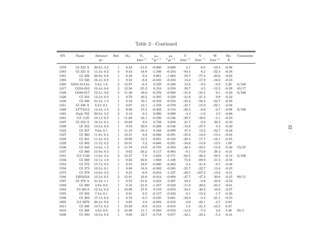
–32

–

Table 2—Continued

NN Name distance Ref. MV Vr µα µδ U V W Hα Comments

pc. kms−1 ′′yr−1 ′′yr−1 kms−1 kms−1 kms−1 A

1379 Gl 323 A 20.0± 3.2 1 8.43 -11.8 -0.060 0.000 4.1 6.9 -10.4 -0.36

1385 Gl 325 A 11.3± 0.3 3 8.43 44.9 -1.340 -0.354 -83.4 8.2 -22.4 -0.58

1391 Gl 328 20.0± 0.8 1 8.49 0.4 0.061 -1.064 50.7 -77.4 -40.6 -0.62

1395 Gl 330 16.4± 0.8 1 9.52 -8.6 -0.035 -0.333 13.2 -17.9 -16.0 -0.33

1405 G041-014Aa 5.6± 1.6 2 12.87 -6.4 0.329 -0.320 13.2 -3.9 -0.2 2.20 0/100

1417 G234-053 10.4± 0.6 2 12.56 -25.2 0.216 0.359 29.7 4.5 -12.5 -0.29 83/17

1420 G046-017 12.3± 3.6 2 11.36 49.0 -0.376 -0.080 -41.0 -34.5 6.1 -0.33 0/100

1426 Gl 334 14.5± 0.3 1 8.70 40.2 -0.305 0.220 -41.6 -21.3 9.8 -0.42

1439 Gl 336 21.2± 1.3 1 8.33 10.1 -0.322 -0.552 -23.2 -56.3 -22.7 -0.56

1451 Gl 338 A 6.2± 0.1 1 8.67 12.1 -1.558 -0.579 -42.7 -15.0 -22.1 -0.56

1460 LTT3412 14.4± 4.3 2 9.96 15.5 -0.302 0.154 -26.3 -8.6 -2.7 -0.08 0/100

1465 Stph 762 20.0± 3.2 3 8.13 6.5 0.000 0.000 -4.4 -1.6 4.5 -0.66

1501 GJ 1125 10.1± 0.3 1 11.68 44.1 -0.590 -0.526 -29.7 -49.6 -5.1 -0.33

1507 Gl 352 A 10.5± 0.4 1 10.69 9.5 0.729 0.059 21.7 -3.9 30.5 -0.33

1509 Gl 353 13.5± 0.3 1 9.53 20.8 -0.208 -0.546 -19.8 -37.5 5.4 -0.40

1522 Gl 357 9.0± 0.1 1 11.16 -33.4 0.168 -0.899 37.4 13.2 -32.7 -0.32

1527 Gl 360 11.8± 0.4 1 10.21 6.0 -0.666 -0.291 -35.9 -14.9 -13.4 -0.04

1528 Gl 361 11.4± 0.2 1 10.09 12.5 -0.621 -0.184 -28.4 -17.7 -16.1 -0.35

1529 Gl 362 11.5± 0.2 1 10.91 5.2 -0.666 -0.291 -34.6 -14.9 -13.5 1.09

1530 Gl 363 14.0± 1.3 2 11.78 13.0 -0.735 -0.502 -48.4 -33.5 -13.9 -0.30 73/27

1537 Gl 366 15.9± 0.3 1 9.62 -26.2 0.117 -0.984 -0.1 -74.6 26.4 -0.41

1541 GJ 1129 11.6± 3.4 2 12.27 7.9 -1.624 -0.171 -64.5 -20.4 -59.5 -0.14 0/100

1550 Gl 369 12.1± 1.0 1 9.63 60.8 1.068 -1.438 75.6 -89.9 21.5 -0.45

1554 Gl 372 15.7± 0.3 1 9.55 24.0 -0.090 -0.462 3.4 -41.8 -6.7 -0.38

1558 Gl 373 10.5± 0.1 1 8.89 16.9 -0.302 -0.585 -25.7 -22.7 13.4 -0.45

1575 Gl 378 14.9± 0.3 1 9.21 -6.9 -0.634 -1.437 -26.5 -107.2 -13.0 -0.51

1586 LHS2224 13.5± 0.5 2 12.81 43.9 -0.454 -0.808 -47.7 -47.3 30.6 -0.25 89/11

1587 Gl 379 A 21.2± 1.1 1 8.55 -51.6 0.224 0.267 52.3 -2.8 -33.9 -0.52

1592 Gl 380 4.9± 0.0 1 8.16 -21.9 -1.357 -0.523 -11.9 -20.6 -32.5 -0.61

1594 Gl 381A 12.3± 0.2 1 10.90 27.0 0.510 -0.653 34.5 -40.2 16.0 -0.37

1595 Gl 382 7.8± 0.1 1 9.81 8.9 -0.157 -0.232 -3.1 -13.2 -1.7 -0.30

1596 Gl 383 17.1± 0.3 1 8.78 -2.5 -0.525 0.001 -34.0 -5.4 -25.1 -0.55

1605 GJ 2079 20.4± 0.6 1 8.65 4.9 -0.094 -0.210 -3.0 -22.1 -4.7 0.83

1611 Gl 386 13.7± 0.4 1 10.29 -9.9 -0.415 -0.618 1.8 -21.3 -44.5 0.37

1616 Gl 388 4.9± 0.0 2 10.96 11.1 -0.503 -0.053 -14.2 -7.3 2.6 3.40 95/5

1630 Gl 390 12.5± 0.2 1 9.69 22.7 -0.718 0.077 -42.1 -23.4 -5.3 -0.41

–33

–

Table 2—Continued

NN Name distance Ref. MV Vr µα µδ U V W Hα Comments

pc. kms−1 ′′yr−1 ′′yr−1 kms−1 kms−1 kms−1 A

1642 Gl 393 7.2± 0.1 1 10.34 8.8 -0.587 -0.746 -6.9 -29.1 -15.2 -0.53

1649 Gl 397.1A 17.5± 0.3 1 8.72 -2.9 -0.144 0.206 -9.0 12.3 -14.5 -0.52

1657 LHS 283 12.5± 0.6 2 11.45 -50.4 -1.652 -0.585 -57.1 -77.1 -64.2 -0.22 79/21

1658 Gl 398 13.4± 0.7 2 11.97 19.7 -0.636 0.090 -42.3 -16.2 -2.0 4.40 82/18

1664 GJ 1134 10.3± 0.2 2 12.91 -2.0 -1.461 -0.362 -55.0 -35.5 -33.5 -0.30 92/8

1671 Gl 400 A 14.1± 0.4 1 8.55 -1.8 -0.037 0.156 -3.8 9.4 -3.9 -0.45

1682 GJ 1138 A 9.8± 0.3 2 13.05 58.2 -0.674 -1.030 -39.2 -58.1 41.7 -0.27 89/11

1687 Gl 402 6.9± 0.2 1 12.46 -2.5 -0.815 -0.812 -10.0 -27.8 -23.4 -0.28

1690 Gl 403 13.0± 2.1 2 12.10 19.2 -1.110 0.188 -69.1 -17.3 -10.1 -0.14 65/35

1692 LHS2320 9.9± 2.9 2 14.41 0.2 -0.625 -0.135 -22.2 -13.6 -14.9 6.84 0/100

1709 Gl 408 6.6± 0.1 1 10.91 3.2 -0.402 -0.233 -9.1 -11.4 -3.0 -0.31

1717 Gl 410 11.7± 0.1 1 9.26 -14.2 0.140 -0.059 12.5 3.3 -10.2 0.00

1719 Gl 411 2.5± 0.0 1 10.47 -85.9 -0.569 -4.773 46.1 -52.4 -75.8 -0.20

1723 Gl 412 A 4.8± 0.0 1 10.30 69.6 -4.427 0.949 -122.8 -5.9 18.7 -0.26

1732 Gl 413.1 10.7± 0.1 1 10.30 -4.5 -0.793 -0.449 -24.0 -19.5 -34.6 -0.59

1742 G119-062 13.3± 3.9 2 11.76 3.6 -0.178 0.098 -13.1 1.8 -1.2 4.20 0/100

1746 Stph 928 14.4± 4.2 2 9.97 30.0 0.000 0.000 -7.9 -9.1 27.5 -0.50 0/100

1756 Gl 421 A 16.6± 1.2 1 8.86 9.1 0.140 -0.741 38.7 -34.1 -30.7 -0.72

1762 GJ 1144 17.6± 0.4 1 8.78 -7.8 -0.206 -0.096 -11.2 -4.8 -16.5 -0.4 low-res

1765 GJ 1145 17.6± 0.4 1 8.57 -19.1 0.157 -0.100 12.7 17.5 -11.7 -0.58

1770 Gl 424 9.1± 0.0 1 9.51 61.0 -2.955 0.186 -141.0 -11.7 -1.2 -0.44

1801 Gl 430.1 16.2± 0.3 1 9.25 -5.9 -0.580 0.000 -37.6 -15.9 -18.7 -0.31

1810 LHS2427 17.8± 0.5 1 9.93 -35.0 -0.622 -0.278 -41.1 -3.7 -53.1 -0.4 low-res

1827 GJ 1148 11.0± 0.3 1 11.68 -9.8 -0.600 -0.119 -22.0 -19.6 -15.7 -0.27

1830 Gl 436 10.2± 0.2 1 10.62 7.6 0.757 -0.770 46.4 -19.6 15.6 -0.37

1845 Gl 445 5.4± 0.0 1 12.16 -112.2 0.711 0.489 67.2 -54.7 -74.6 -0.23

1847 G010-049A 13.9± 4.2 2 12.54 6.9 -0.290 -0.089 -13.8 -16.0 -1.3 4.66 0/100

1849 Gl 447 3.3± 0.0 1 13.50 -31.0 0.633 -1.190 17.3 5.9 -32.8 -0.18

1854 GJ 1151 8.3± 0.2 2 13.66 -35.6 -1.536 -0.978 -27.5 -67.5 -33.1 -0.13 93/7

1855 Gl 450 8.6± 0.1 1 10.07 1.0 -0.220 0.272 -12.7 6.2 -2.4 -0.26

1866 Gl 452.1 12.1± 1.8 2 12.35 3.5 0.083 -0.781 25.7 -35.9 -9.5 1.25 70/30

1894 G237-043 12.7± 3.8 2 12.56 4.4 -0.474 -0.067 -25.7 -13.7 1.1 -0.18 0/100

1905 LHS2520 10.1± 2.9 2 12.04 79.5 -0.050 -0.718 31.1 -73.3 34.2 -0.26 0/100

1907 LTT4562 A 12.8± 0.4 1 11.13 -9.1 -0.198 -0.160 -8.8 -4.6 -14.9 -0.30

1915 Gl 458 A 15.3± 0.3 1 8.86 -19.9 0.230 0.082 18.8 6.1 -17.9 -0.58

1923 GJ 1154 A 8.4± 0.3 2 14.11 -13.7 -0.942 -0.288 -28.5 -20.4 -22.3 5.41 90/10

–34

–

Table 2—Continued

NN Name distance Ref. MV Vr µα µδ U V W Hα Comments

pc. kms−1 ′′yr−1 ′′yr−1 kms−1 kms−1 kms−1 A

1934 GJ 1156 6.6± 0.1 2 14.70 5.1 -1.285 0.206 -37.8 -16.0 2.0 6.11 95/5

1937 Gl 461 A 15.2± 4.6 2 9.19 4.0 0.088 -0.020 6.7 0.3 3.6 -0.35 0/100

1938 Gl 462 16.0± 0.3 1 8.42 22.6 0.163 -0.523 24.0 -23.9 33.0 -0.59

1942 G237-064 13.0± 0.9 1 10.68 14.9 0.208 -0.120 7.8 8.9 17.4 -0.23

1943 Gl 464 21.2± 0.8 1 8.75 7.6 0.026 -0.186 12.1 -16.1 2.8 -0.72

1945 Gl 465 8.9± 0.2 1 11.54 51.5 1.082 -2.289 94.4 -65.6 -28.9 -0.28

1952 LTT4730 A 13.4± 4.0 2 10.33 -6.9 -0.281 0.015 -17.5 -4.6 -6.2 0.57 0/100

1954 Gl 469 13.6± 0.5 1 11.39 -10.2 -0.638 -0.288 -27.0 -32.5 -18.8 -0.33

1966 Gl 471 13.4± 0.3 1 9.06 15.1 -0.635 -0.533 -15.7 -52.5 0.7 -0.38

1972 Gl 473 A 4.3± 0.0 2 14.85 2.4 -1.796 0.233 -33.4 -15.8 1.6 4.78 95/5

2009 Gl 486 8.2± 0.2 1 11.80 19.1 -0.990 -0.424 -20.7 -39.0 13.0 -0.28

2017 Gl 487 Aa 10.2± 0.1 1 12.05 -16.0 -0.427 -0.091 -10.0 -22.5 -9.8 0.20

2024 Gl 488 10.8± 0.1 1 8.33 6.7 -0.039 -0.400 9.9 -18.9 -3.7 -0.65

2043 Gl 493.1 8.4± 0.3 2 13.78 -25.5 -0.942 0.242 -42.1 -6.4 -18.4 4.59 92/8

2045 Gl 494 A 11.4± 0.1 1 9.46 -12.2 -0.714 -0.021 -33.4 -20.4 -10.3 1.09

2051 Gl 499 A 18.6± 0.7 1 8.09 1.2 -0.059 0.060 -7.1 1.3 2.2 -0.33

2093 Gl 507 A 13.2± 0.5 1 8.91 -15.1 0.374 -0.789 48.2 -27.7 -11.2 -0.47

2096 Gl 507.1 17.4± 0.7 1 9.42 -13.2 -0.217 -0.125 -8.5 -20.7 -9.9 -0.54

2097 Gl 508 Aa 10.4± 0.2 1 9.50 1.9 0.144 -0.028 6.3 3.9 1.4 -0.46

2100 Gl 508.2 16.1± 0.3 1 9.59 -39.8 0.518 -0.288 43.6 -0.5 -41.6 -0.46

2102 LHS 350 13.5± 0.4 2 12.28 -18.4 -0.629 -0.878 -1.1 -69.7 -16.0 -0.25 87/13

2107 Gl 509 A 18.5± 0.6 1 8.18 -38.3 -0.486 0.234 -49.6 -13.0 -32.8 -0.59

2112 Gl 510 16.3± 0.5 1 9.95 -29.8 -0.460 -0.103 -42.9 -7.2 -17.9 0.01

2123 Gl 514 7.6± 0.1 1 9.64 15.2 1.111 -1.084 57.2 -8.6 -3.5 -0.43

2128 G165-008A 10.5± 3.2 2 12.20 -7.5 -0.228 -0.159 -4.8 -14.0 -5.3 9.00 0/100

2137 GJ 1172 20.5± 0.6 1 8.41 13.7 0.139 -0.132 22.1 -4.4 5.0 -0.57

2150 Gl 519 10.9± 0.1 1 8.86 -14.4 0.309 -0.060 13.4 4.3 -16.6 -0.53

2151 Gl 520 A 21.9± 1.1 1 8.47 -21.1 -0.211 -0.112 -7.7 -29.5 -11.4 -0.49

2156 Gl 521 13.3± 0.3 1 9.62 -60.7 -0.047 0.399 -15.2 -5.9 -63.7 -0.44

2157 Gl 521.1 14.5± 0.3 1 8.78 28.8 -0.384 0.495 -22.1 -0.6 46.8 -0.56

2168 LHS2784 9.1± 0.2 1 12.16 6.6 -0.106 -0.700 16.7 -24.4 10.1 -0.21

2173 Gl 525 13.0± 0.1 1 9.23 18.9 0.436 -1.845 93.3 -72.4 -7.6 -0.44

2175 LHS2794 11.4± 0.5 1 11.57 5.0 -0.313 -0.538 -0.5 -31.2 -13.4 -0.28

2176 Gl 526 5.4± 0.0 1 9.79 16.0 1.786 -1.488 61.5 -2.0 -3.3 -0.45

2198 Gl 532 14.0± 0.1 1 8.17 -46.5 0.423 -0.147 30.5 -8.5 -45.2 -0.58

2201 Gl 533 A 20.9± 0.6 1 8.25 -10.5 -0.174 -0.673 22.1 -62.0 -22.8 -0.76

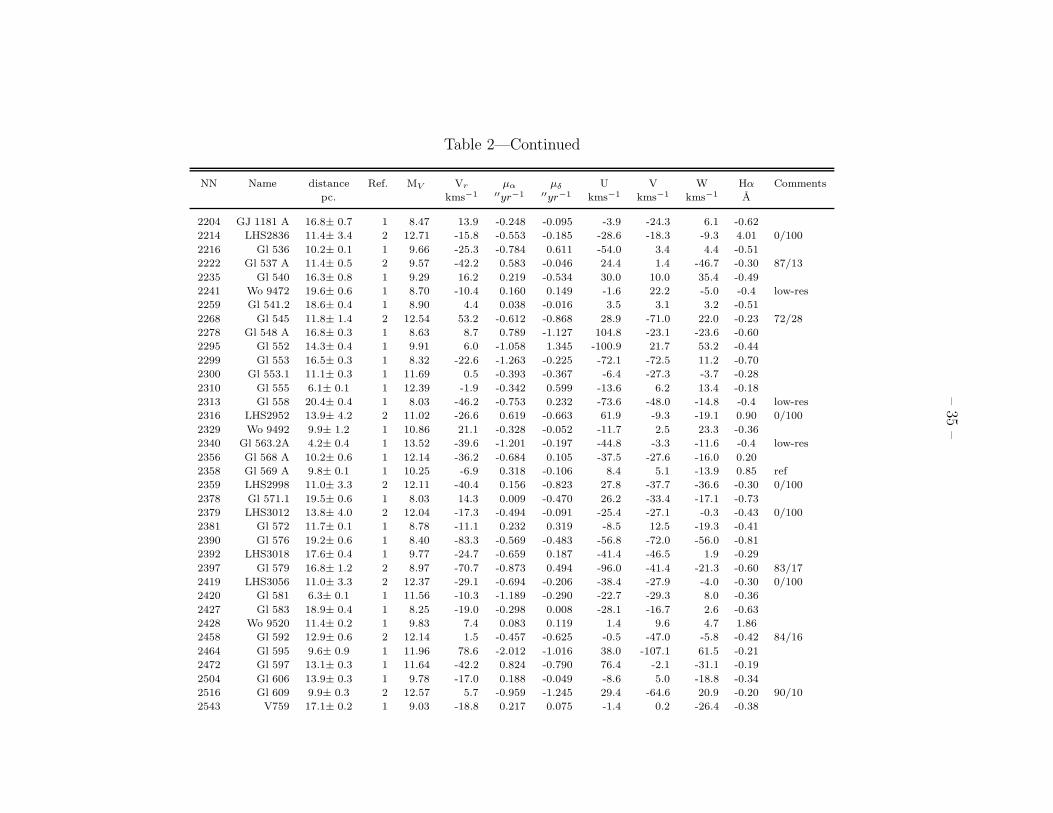
–35

–

Table 2—Continued

NN Name distance Ref. MV Vr µα µδ U V W Hα Comments

pc. kms−1 ′′yr−1 ′′yr−1 kms−1 kms−1 kms−1 A

2204 GJ 1181 A 16.8± 0.7 1 8.47 13.9 -0.248 -0.095 -3.9 -24.3 6.1 -0.62

2214 LHS2836 11.4± 3.4 2 12.71 -15.8 -0.553 -0.185 -28.6 -18.3 -9.3 4.01 0/100

2216 Gl 536 10.2± 0.1 1 9.66 -25.3 -0.784 0.611 -54.0 3.4 4.4 -0.51

2222 Gl 537 A 11.4± 0.5 2 9.57 -42.2 0.583 -0.046 24.4 1.4 -46.7 -0.30 87/13

2235 Gl 540 16.3± 0.8 1 9.29 16.2 0.219 -0.534 30.0 10.0 35.4 -0.49

2241 Wo 9472 19.6± 0.6 1 8.70 -10.4 0.160 0.149 -1.6 22.2 -5.0 -0.4 low-res

2259 Gl 541.2 18.6± 0.4 1 8.90 4.4 0.038 -0.016 3.5 3.1 3.2 -0.51

2268 Gl 545 11.8± 1.4 2 12.54 53.2 -0.612 -0.868 28.9 -71.0 22.0 -0.23 72/28

2278 Gl 548 A 16.8± 0.3 1 8.63 8.7 0.789 -1.127 104.8 -23.1 -23.6 -0.60

2295 Gl 552 14.3± 0.4 1 9.91 6.0 -1.058 1.345 -100.9 21.7 53.2 -0.44

2299 Gl 553 16.5± 0.3 1 8.32 -22.6 -1.263 -0.225 -72.1 -72.5 11.2 -0.70

2300 Gl 553.1 11.1± 0.3 1 11.69 0.5 -0.393 -0.367 -6.4 -27.3 -3.7 -0.28

2310 Gl 555 6.1± 0.1 1 12.39 -1.9 -0.342 0.599 -13.6 6.2 13.4 -0.18

2313 Gl 558 20.4± 0.4 1 8.03 -46.2 -0.753 0.232 -73.6 -48.0 -14.8 -0.4 low-res

2316 LHS2952 13.9± 4.2 2 11.02 -26.6 0.619 -0.663 61.9 -9.3 -19.1 0.90 0/100

2329 Wo 9492 9.9± 1.2 1 10.86 21.1 -0.328 -0.052 -11.7 2.5 23.3 -0.36

2340 Gl 563.2A 4.2± 0.4 1 13.52 -39.6 -1.201 -0.197 -44.8 -3.3 -11.6 -0.4 low-res

2356 Gl 568 A 10.2± 0.6 1 12.14 -36.2 -0.684 0.105 -37.5 -27.6 -16.0 0.20

2358 Gl 569 A 9.8± 0.1 1 10.25 -6.9 0.318 -0.106 8.4 5.1 -13.9 0.85 ref

2359 LHS2998 11.0± 3.3 2 12.11 -40.4 0.156 -0.823 27.8 -37.7 -36.6 -0.30 0/100

2378 Gl 571.1 19.5± 0.6 1 8.03 14.3 0.009 -0.470 26.2 -33.4 -17.1 -0.73

2379 LHS3012 13.8± 4.0 2 12.04 -17.3 -0.494 -0.091 -25.4 -27.1 -0.3 -0.43 0/100

2381 Gl 572 11.7± 0.1 1 8.78 -11.1 0.232 0.319 -8.5 12.5 -19.3 -0.41

2390 Gl 576 19.2± 0.6 1 8.40 -83.3 -0.569 -0.483 -56.8 -72.0 -56.0 -0.81

2392 LHS3018 17.6± 0.4 1 9.77 -24.7 -0.659 0.187 -41.4 -46.5 1.9 -0.29

2397 Gl 579 16.8± 1.2 2 8.97 -70.7 -0.873 0.494 -96.0 -41.4 -21.3 -0.60 83/17

2419 LHS3056 11.0± 3.3 2 12.37 -29.1 -0.694 -0.206 -38.4 -27.9 -4.0 -0.30 0/100

2420 Gl 581 6.3± 0.1 1 11.56 -10.3 -1.189 -0.290 -22.7 -29.3 8.0 -0.36

2427 Gl 583 18.9± 0.4 1 8.25 -19.0 -0.298 0.008 -28.1 -16.7 2.6 -0.63

2428 Wo 9520 11.4± 0.2 1 9.83 7.4 0.083 0.119 1.4 9.6 4.7 1.86

2458 Gl 592 12.9± 0.6 2 12.14 1.5 -0.457 -0.625 -0.5 -47.0 -5.8 -0.42 84/16

2464 Gl 595 9.6± 0.9 1 11.96 78.6 -2.012 -1.016 38.0 -107.1 61.5 -0.21

2472 Gl 597 13.1± 0.3 1 11.64 -42.2 0.824 -0.790 76.4 -2.1 -31.1 -0.19

2504 Gl 606 13.9± 0.3 1 9.78 -17.0 0.188 -0.049 -8.6 5.0 -18.8 -0.34

2516 Gl 609 9.9± 0.3 2 12.57 5.7 -0.959 -1.245 29.4 -64.6 20.9 -0.20 90/10

2543 V759 17.1± 0.2 1 9.03 -18.8 0.217 0.075 -1.4 0.2 -26.4 -0.38

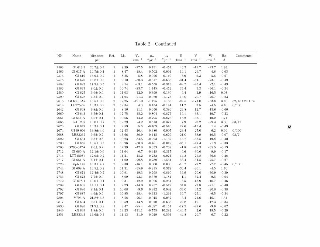
–36

–

Table 2—Continued

NN Name distance Ref. MV Vr µα µδ U V W Hα Comments

pc. kms−1 ′′yr−1 ′′yr−1 kms−1 kms−1 kms−1 A

2563 Gl 616.2 20.7± 0.4 1 8.39 -27.5 0.191 -0.454 46.2 -19.7 -23.7 1.93

2566 Gl 617 A 10.7± 0.1 1 8.47 -18.4 -0.502 0.091 -10.1 -29.7 4.6 -0.63

2576 Gl 619 15.9± 0.2 1 8.25 5.8 -0.026 0.119 -6.9 6.3 5.5 -0.67

2578 Gl 620 16.8± 0.5 1 9.10 -30.3 -0.317 -0.638 -31.4 -51.1 -23.1 -0.49

2582 Gl 622 17.9± 0.5 1 9.14 -63.1 -0.558 -0.313 -69.7 -45.4 -2.1 -0.43

2583 Gl 623 8.0± 0.0 1 10.74 -23.7 1.145 -0.453 24.4 5.2 -46.1 -0.24

2589 Gl 625 6.6± 0.0 1 11.03 -12.0 0.399 -0.130 6.4 -1.9 -16.5 0.03

2599 Gl 628 4.3± 0.0 1 11.94 -21.3 -0.070 -1.173 -13.0 -20.7 -20.7 -0.23

2616 Gl 630.1Aa 13.5± 0.5 2 12.25 -191.0 -1.125 1.165 -99.5 -174.0 -83.8 3.40 82/18 CM Dra

2618 LP275-68 13.3± 3.9 2 12.34 4.0 0.134 -0.144 11.7 3.5 -4.5 4.10 0/100

2642 Gl 638 9.8± 0.0 1 8.16 -31.1 -0.050 0.386 -29.8 -12.7 -15.6 -0.66

2660 Gl 643 6.5± 0.1 1 12.75 15.2 -0.804 -0.877 19.1 -33.1 10.7 -0.23

2661 Gl 644 A 6.5± 0.1 1 10.66 14.2 -0.795 -0.876 18.2 -33.1 10.2 1.71

2665 GJ 1207 10.0± 0.7 2 12.29 -4.2 0.513 -0.377 7.9 -0.2 -29.4 3.30 83/17

2673 Gl 649 10.3± 0.1 1 9.59 5.6 -0.109 -0.516 22.6 -13.4 1.4 -0.49

2674 G139-003 13.8± 4.0 2 12.43 -26.4 -0.380 0.007 -23.4 -27.0 6.2 0.99 0/100

2688 LHS3262 9.6± 0.2 2 13.66 36.9 0.145 0.629 -21.0 38.9 16.5 -0.07 93/7

2692 Gl 654 9.3± 0.8 1 10.23 34.5 -0.923 -1.132 45.7 -53.5 19.8 -0.40

2700 Gl 655 13.5± 0.5 1 10.96 -50.3 -0.481 -0.012 -35.1 -47.4 -1.9 -0.33

2708 G203-047A 7.6± 0.2 1 12.39 -42.8 0.333 -0.269 -1.8 -28.3 -35.5 -0.13

2712 Gl 660 A 12.1± 0.6 1 11.64 -6.7 -0.448 -0.317 -0.6 -30.6 9.9 -0.17

2714 LTT15087 12.0± 0.2 1 11.21 -45.2 0.232 -0.024 -14.3 -25.8 -36.8 -0.28

2717 Gl 661 A 6.1± 0.1 1 11.02 -29.8 0.239 -1.564 36.4 -31.5 -25.7 -0.27

2728 Stph 145 16.3± 4.7 2 9.30 -16.1 0.000 0.000 -10.7 -9.2 -7.7 -0.45 0/100

2744 Gl 669 A 10.5± 0.2 1 11.31 -35.9 -0.215 0.372 -36.4 -20.1 -4.5 1.76

2748 Gl 671 12.4± 0.2 1 10.91 -19.3 0.298 -0.810 39.9 -20.0 -30.9 -0.39

2756 Gl 673 7.7± 0.0 1 8.09 -23.1 -0.579 -1.181 1.1 -52.4 -9.5 -0.64

2772 Gl 678.1 10.0± 0.1 1 9.31 -12.9 0.026 -0.261 -3.5 -13.9 -10.7 -0.46

2789 Gl 685 14.1± 0.1 1 9.23 -14.0 0.257 -0.512 34.8 -2.8 -21.1 -0.40

2792 Gl 686 8.1± 0.1 1 10.08 -9.6 0.932 0.992 -34.0 35.2 -20.8 -0.38

2797 Gl 687 4.6± 0.0 1 10.85 -28.4 -0.333 -1.261 30.7 -25.1 -6.5 -0.34

2804 V796 A 21.8± 6.3 1 8.58 -26.1 -0.045 0.052 -5.4 -24.6 -10.1 1.31

2817 Gl 694 9.5± 0.1 1 10.59 -14.8 0.010 -0.636 22.8 -19.1 -12.4 -0.34

2830 Gl 696 21.9± 0.9 1 8.47 -25.4 -0.027 -0.151 -17.2 -22.6 -9.6 -0.62

2849 Gl 699 1.8± 0.0 1 13.23 -111.1 -0.755 10.282 -140.5 2.6 18.5 -0.20

2851 LHS3343 13.6± 0.3 1 11.13 -31.9 -0.029 0.593 -44.8 -20.7 -6.7 -0.22

–37

–

Table 2—Continued

NN Name distance Ref. MV Vr µα µδ U V W Hα Comments

pc. kms−1 ′′yr−1 ′′yr−1 kms−1 kms−1 kms−1 A

2859 Gl 701 7.8± 0.1 1 9.93 32.5 0.551 -0.333 32.7 14.1 -18.8 -0.45

2865 GJ 1224 7.7± 0.2 2 14.20 -34.8 -0.564 -0.350 -28.9 -29.1 10.8 3.01 93/7

2882 Gl 708.2 19.0± 1.3 1 8.81 7.5 0.084 -0.494 34.6 -18.7 -23.4 -0.51

2885 Gl 709 17.1± 0.2 1 9.12 -36.1 -0.031 0.298 -32.2 -28.3 -7.2 -0.54

2888 LHS 462 A 11.5± 0.5 2 11.57 0.1 -0.334 -1.039 54.5 -23.8 0.0 -0.29 89/11

2892 Gl 710 19.3± 0.4 1 8.23 -13.5 -0.013 -0.005 -11.5 -7.2 -0.5 -0.60

2897 LHS3376 7.5± 0.2 2 14.09 5.0 0.468 -0.411 11.6 14.1 -13.5 2.14 92/8

2901 LTT15435 13.0± 3.9 2 11.93 -21.8 -0.068 -0.177 -1.8 -23.7 -6.8 -0.23 0/100

2904 GJ 1227 8.3± 0.1 2 13.82 -14.4 -0.931 -1.231 53.8 -24.8 19.7 -0.17 96/4

2916 G205-028 11.9± 3.6 2 11.61 -18.2 -0.087 0.410 -26.5 -12.7 5.1 -0.15 0/100

2921 LP229-17 7.2± 2.1 2 12.14 12.4 0.046 -0.218 10.7 9.8 0.5 -0.22 0/100

2923 Gl 720 A 15.5± 0.2 1 8.90 -30.4 0.452 0.341 -37.9 -9.7 -33.5 -0.51

2925 G141-021 11.0± 3.2 2 12.24 -43.3 0.194 0.288 -43.0 -16.4 -9.2 0.47 0/100

2928 GJ 2138 12.7± 0.4 1 10.74 -39.7 0.123 -0.530 -30.8 -37.0 -18.1 -0.30

2933 Gl 724 16.2± 0.5 1 9.58 -32.6 -0.078 -0.666 -15.2 -57.0 -15.5 -0.50

2935 GJ 1230 Aa 7.3± 1.2 2 13.78 -37.6 0.499 0.041 -26.2 -22.2 -23.0 2.10 55/45

2940 G206-040 11.4± 0.2 1 10.99 -30.1 -0.307 0.011 -10.8 -31.9 6.9 -0.32

2942 G141-029 11.6± 3.4 2 12.49 -33.2 -0.044 0.310 -34.3 -14.0 5.2 4.19 0/100

2945 Gl 725 A 3.5± 0.0 1 11.19 -1.3 -1.358 1.822 -24.3 -12.7 25.9 -0.31

2947 LTT7434 10.3± 3.0 2 12.59 -32.0 0.297 -0.318 -34.2 -12.1 -12.4 -0.34 0/100

2953 Gl 726 14.1± 0.1 1 8.10 12.4 -0.121 -0.247 19.9 -9.8 -0.7 -0.59

2958 Gl 728 17.1± 0.3 1 8.05 -22.0 -0.413 -0.425 18.5 -48.1 11.6 -0.67

2960 Gl 729 3.0± 0.0 1 13.08 -10.9 0.690 -0.207 -12.7 -1.1 -7.9 1.80

2964 G205-038 13.0± 3.8 2 11.95 -76.9 0.251 -0.117 -12.6 -65.5 -41.9 -0.33 0/100

2966 Gl 731 15.6± 0.3 1 9.18 -10.5 -0.251 -0.475 22.5 -34.4 -0.4 -0.46

2974 Gl 734 A 15.5± 1.7 2 8.49 -24.1 0.120 -0.010 -19.4 -13.7 -9.7 -0.69 69/31

2976 Gl 735 11.6± 0.2 1 9.79 -6.2 0.101 -0.082 -3.5 -5.0 -7.3 2.10

2988 Gl 740 11.1± 0.1 1 9.00 11.2 -0.208 -1.228 48.3 -41.0 -20.0 -0.61

3004 Gl 745 A 8.6± 0.2 1 11.09 33.0 -0.472 -0.334 35.6 13.1 14.1 -0.20

3009 Gl 747 A 8.3± 0.1 2 12.27 -47.3 1.232 1.075 -71.4 -11.8 -33.7 -0.21 97/3

3013 G207-019 12.4± 3.7 2 11.33 -1.7 -0.220 -0.220 14.3 -10.0 5.6 -0.34 0/100

3024 Gl 748 9.6± 0.2 1 11.18 -41.4 1.733 -0.490 -47.1 -15.6 -77.2 -0.26

3037 Gl 752 A 5.9± 0.0 1 10.27 36.3 -0.601 -1.337 54.0 -7.4 -5.1 -0.42

3049 GJ 1236 11.2± 0.2 2 12.10 27.3 -0.740 -0.389 46.3 -7.1 22.8 -0.25 95/5

3074 Gl 763 14.5± 0.3 1 8.55 -59.8 0.523 0.303 -69.9 -15.7 -13.2 -0.55

3100 Gl 766 A 10.9± 0.5 2 12.73 -5.6 -0.032 -1.226 47.2 -29.4 -30.9 -0.19 84/16

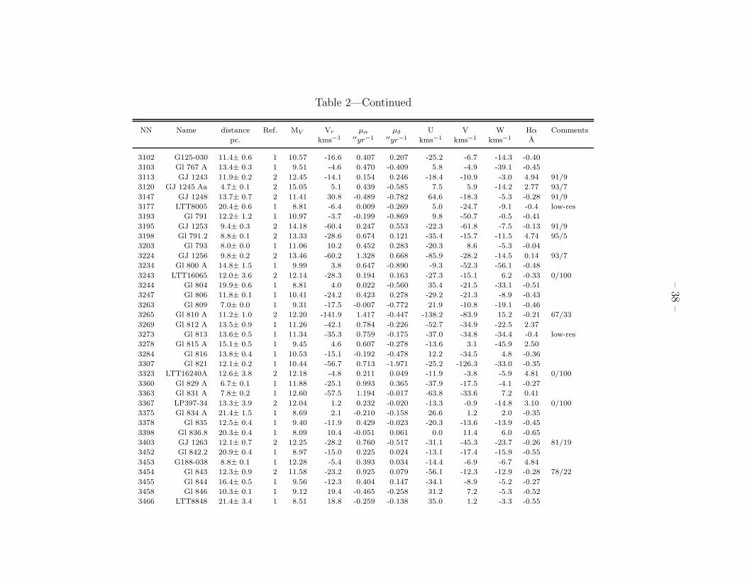
–38

–

Table 2—Continued

NN Name distance Ref. MV Vr µα µδ U V W Hα Comments

pc. kms−1 ′′yr−1 ′′yr−1 kms−1 kms−1 kms−1 A

3102 G125-030 11.4± 0.6 1 10.57 -16.6 0.407 0.207 -25.2 -6.7 -14.3 -0.40

3103 Gl 767 A 13.4± 0.3 1 9.51 -4.6 0.470 -0.409 5.8 -4.9 -39.1 -0.45

3113 GJ 1243 11.9± 0.2 2 12.45 -14.1 0.154 0.246 -18.4 -10.9 -3.0 4.94 91/9

3120 GJ 1245 Aa 4.7± 0.1 2 15.05 5.1 0.439 -0.585 7.5 5.9 -14.2 2.77 93/7

3147 GJ 1248 13.7± 0.7 2 11.41 30.8 -0.489 -0.782 64.6 -18.3 -5.3 -0.28 91/9

3177 LTT8005 20.4± 0.6 1 8.81 -6.4 0.009 -0.269 5.0 -24.7 -9.1 -0.4 low-res

3193 Gl 791 12.2± 1.2 1 10.97 -3.7 -0.199 -0.869 9.8 -50.7 -0.5 -0.41

3195 GJ 1253 9.4± 0.3 2 14.18 -60.4 0.247 0.553 -22.3 -61.8 -7.5 -0.13 91/9

3198 Gl 791.2 8.8± 0.1 2 13.33 -28.6 0.674 0.121 -35.4 -15.7 -11.5 4.74 95/5

3203 Gl 793 8.0± 0.0 1 11.06 10.2 0.452 0.283 -20.3 8.6 -5.3 -0.04

3224 GJ 1256 9.8± 0.2 2 13.46 -60.2 1.328 0.668 -85.9 -28.2 -14.5 0.14 93/7

3234 Gl 800 A 14.8± 1.5 1 9.99 3.8 0.647 -0.890 -9.3 -52.3 -56.1 -0.48

3243 LTT16065 12.0± 3.6 2 12.14 -28.3 0.194 0.163 -27.3 -15.1 6.2 -0.33 0/100

3244 Gl 804 19.9± 0.6 1 8.81 4.0 0.022 -0.560 35.4 -21.5 -33.1 -0.51

3247 Gl 806 11.8± 0.1 1 10.41 -24.2 0.423 0.278 -29.2 -21.3 -8.9 -0.43

3263 Gl 809 7.0± 0.0 1 9.31 -17.5 -0.007 -0.772 21.9 -10.8 -19.1 -0.46

3265 Gl 810 A 11.2± 1.0 2 12.20 -141.9 1.417 -0.447 -138.2 -83.9 15.2 -0.21 67/33

3269 Gl 812 A 13.5± 0.9 1 11.26 -42.1 0.784 -0.226 -52.7 -34.9 -22.5 2.37

3273 Gl 813 13.6± 0.5 1 11.34 -35.3 0.759 -0.175 -37.0 -34.8 -34.4 -0.4 low-res

3278 Gl 815 A 15.1± 0.5 1 9.45 4.6 0.607 -0.278 -13.6 3.1 -45.9 2.50

3284 Gl 816 13.8± 0.4 1 10.53 -15.1 -0.192 -0.478 12.2 -34.5 4.8 -0.36

3307 Gl 821 12.1± 0.2 1 10.44 -56.7 0.713 -1.971 -25.2 -126.3 -33.0 -0.35

3323 LTT16240A 12.6± 3.8 2 12.18 -4.8 0.211 0.049 -11.9 -3.8 -5.9 4.81 0/100

3360 Gl 829 A 6.7± 0.1 1 11.88 -25.1 0.993 0.365 -37.9 -17.5 -4.1 -0.27

3363 Gl 831 A 7.8± 0.2 1 12.60 -57.5 1.194 -0.017 -63.8 -33.6 7.2 0.41

3367 LP397-34 13.3± 3.9 2 12.04 1.2 0.232 -0.020 -13.3 -0.9 -14.8 3.10 0/100

3375 Gl 834 A 21.4± 1.5 1 8.69 2.1 -0.210 -0.158 26.6 1.2 2.0 -0.35

3378 Gl 835 12.5± 0.4 1 9.40 -11.9 0.429 -0.023 -20.3 -13.6 -13.9 -0.45

3398 Gl 836.8 20.3± 0.4 1 8.09 10.4 -0.051 0.061 0.0 11.4 6.0 -0.65

3403 GJ 1263 12.1± 0.7 2 12.25 -28.2 0.760 -0.517 -31.1 -45.3 -23.7 -0.26 81/19

3452 Gl 842.2 20.9± 0.4 1 8.97 -15.0 0.225 0.024 -13.1 -17.4 -15.9 -0.55

3453 G188-038 8.8± 0.1 1 12.28 -5.4 0.393 0.034 -14.4 -6.9 -6.7 4.84

3454 Gl 843 12.3± 0.9 2 11.58 -23.2 0.925 0.079 -56.1 -12.3 -12.9 -0.28 78/22

3455 Gl 844 16.4± 0.5 1 9.56 -12.3 0.404 0.147 -34.1 -8.9 -5.2 -0.27

3458 Gl 846 10.3± 0.1 1 9.12 19.4 -0.465 -0.258 31.2 7.2 -5.3 -0.52

3466 LTT8848 21.4± 3.4 1 8.51 18.8 -0.259 -0.138 35.0 1.2 -3.3 -0.55

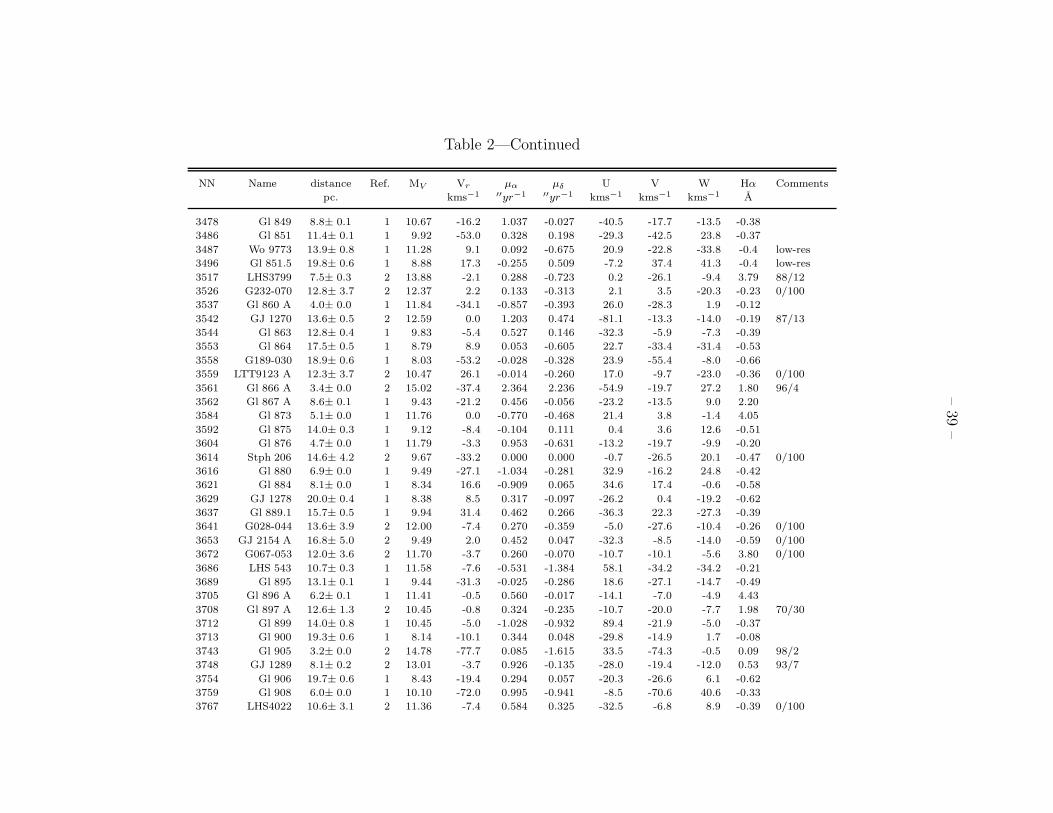
–39

–

Table 2—Continued

NN Name distance Ref. MV Vr µα µδ U V W Hα Comments

pc. kms−1 ′′yr−1 ′′yr−1 kms−1 kms−1 kms−1 A

3478 Gl 849 8.8± 0.1 1 10.67 -16.2 1.037 -0.027 -40.5 -17.7 -13.5 -0.38

3486 Gl 851 11.4± 0.1 1 9.92 -53.0 0.328 0.198 -29.3 -42.5 23.8 -0.37

3487 Wo 9773 13.9± 0.8 1 11.28 9.1 0.092 -0.675 20.9 -22.8 -33.8 -0.4 low-res

3496 Gl 851.5 19.8± 0.6 1 8.88 17.3 -0.255 0.509 -7.2 37.4 41.3 -0.4 low-res

3517 LHS3799 7.5± 0.3 2 13.88 -2.1 0.288 -0.723 0.2 -26.1 -9.4 3.79 88/12

3526 G232-070 12.8± 3.7 2 12.37 2.2 0.133 -0.313 2.1 3.5 -20.3 -0.23 0/100

3537 Gl 860 A 4.0± 0.0 1 11.84 -34.1 -0.857 -0.393 26.0 -28.3 1.9 -0.12

3542 GJ 1270 13.6± 0.5 2 12.59 0.0 1.203 0.474 -81.1 -13.3 -14.0 -0.19 87/13

3544 Gl 863 12.8± 0.4 1 9.83 -5.4 0.527 0.146 -32.3 -5.9 -7.3 -0.39

3553 Gl 864 17.5± 0.5 1 8.79 8.9 0.053 -0.605 22.7 -33.4 -31.4 -0.53

3558 G189-030 18.9± 0.6 1 8.03 -53.2 -0.028 -0.328 23.9 -55.4 -8.0 -0.66

3559 LTT9123 A 12.3± 3.7 2 10.47 26.1 -0.014 -0.260 17.0 -9.7 -23.0 -0.36 0/100

3561 Gl 866 A 3.4± 0.0 2 15.02 -37.4 2.364 2.236 -54.9 -19.7 27.2 1.80 96/4

3562 Gl 867 A 8.6± 0.1 1 9.43 -21.2 0.456 -0.056 -23.2 -13.5 9.0 2.20

3584 Gl 873 5.1± 0.0 1 11.76 0.0 -0.770 -0.468 21.4 3.8 -1.4 4.05

3592 Gl 875 14.0± 0.3 1 9.12 -8.4 -0.104 0.111 0.4 3.6 12.6 -0.51

3604 Gl 876 4.7± 0.0 1 11.79 -3.3 0.953 -0.631 -13.2 -19.7 -9.9 -0.20

3614 Stph 206 14.6± 4.2 2 9.67 -33.2 0.000 0.000 -0.7 -26.5 20.1 -0.47 0/100

3616 Gl 880 6.9± 0.0 1 9.49 -27.1 -1.034 -0.281 32.9 -16.2 24.8 -0.42

3621 Gl 884 8.1± 0.0 1 8.34 16.6 -0.909 0.065 34.6 17.4 -0.6 -0.58

3629 GJ 1278 20.0± 0.4 1 8.38 8.5 0.317 -0.097 -26.2 0.4 -19.2 -0.62

3637 Gl 889.1 15.7± 0.5 1 9.94 31.4 0.462 0.266 -36.3 22.3 -27.3 -0.39

3641 G028-044 13.6± 3.9 2 12.00 -7.4 0.270 -0.359 -5.0 -27.6 -10.4 -0.26 0/100

3653 GJ 2154 A 16.8± 5.0 2 9.49 2.0 0.452 0.047 -32.3 -8.5 -14.0 -0.59 0/100

3672 G067-053 12.0± 3.6 2 11.70 -3.7 0.260 -0.070 -10.7 -10.1 -5.6 3.80 0/100

3686 LHS 543 10.7± 0.3 1 11.58 -7.6 -0.531 -1.384 58.1 -34.2 -34.2 -0.21

3689 Gl 895 13.1± 0.1 1 9.44 -31.3 -0.025 -0.286 18.6 -27.1 -14.7 -0.49

3705 Gl 896 A 6.2± 0.1 1 11.41 -0.5 0.560 -0.017 -14.1 -7.0 -4.9 4.43

3708 Gl 897 A 12.6± 1.3 2 10.45 -0.8 0.324 -0.235 -10.7 -20.0 -7.7 1.98 70/30

3712 Gl 899 14.0± 0.8 1 10.45 -5.0 -1.028 -0.932 89.4 -21.9 -5.0 -0.37

3713 Gl 900 19.3± 0.6 1 8.14 -10.1 0.344 0.048 -29.8 -14.9 1.7 -0.08

3743 Gl 905 3.2± 0.0 2 14.78 -77.7 0.085 -1.615 33.5 -74.3 -0.5 0.09 98/2

3748 GJ 1289 8.1± 0.2 2 13.01 -3.7 0.926 -0.135 -28.0 -19.4 -12.0 0.53 93/7

3754 Gl 906 19.7± 0.6 1 8.43 -19.4 0.294 0.057 -20.3 -26.6 6.1 -0.62

3759 Gl 908 6.0± 0.0 1 10.10 -72.0 0.995 -0.941 -8.5 -70.6 40.6 -0.33

3767 LHS4022 10.6± 3.1 2 11.36 -7.4 0.584 0.325 -32.5 -6.8 8.9 -0.39 0/100

–40

–

Table 2—Continued

NN Name distance Ref. MV Vr µα µδ U V W Hα Comments

pc. kms−1 ′′yr−1 ′′yr−1 kms−1 kms−1 kms−1 A

3782 Gl 912 17.2± 3.4 1 9.96 17.1 -0.460 -0.354 46.8 0.8 -18.4 -0.37

3786 GJ 1292 13.1± 0.4 2 11.13 -32.4 1.032 -1.032 -21.0 -84.1 -41.8 -0.24 85/15

3791 Gl 913 17.4± 0.7 1 8.43 7.6 0.642 -0.003 -49.2 -17.0 -12.4 -0.50

Note. — Column 1 lists the identifier from the PMSU1 tables; Column 2 gives the pCNS3 name;

Column 3 lists the distance estimate and associated uncertainty - an uncertainty of ±0.0km s−1 indicates εd < 0.1 parsecs;

Column 4 gives the source of the distance estimate:

1 - trigonometric parallax from the Hipparcos catalogue (ESA, 1997)

2 - PMSU1 (Reid et al., 1995). The relative weights given to trigonometric and spectroscopic parallax measurements are listed

in column 13: for example, 85/15 indicates that 85% of the weight rests with πtrig .

3 - trigonometric parallax from pCNS3 (Jahreiss & Gliese, 1991)

Column 5 lists the visual absolute magnitude; Column 6 lists the radial velocity, usually from either PMSU3 or Delfosse et

al.(1998), but see notes to column 13. The echelle data are accurate to ±1 kms−1; the low-resolution data are accurate to ±10

kms−1

Columns 7 and 8 give the proper motion in arcseconds/year from either Hipparcos data (column 4 = 1) or the pCNS3;

Columns 9, 10 and 11 give the derived (U, V, W) space motions;

Column 12 lists the Hα equivalent width, where, following PMSU3, a negative value indicates absorption;

Column 13 lists comments on individual stars:

the relative weights of the trigonometric/spectroscopic parallax measurements contributing to d are given (see above);

‘low-res’ indicates that the star has no PMSU3 echelle observations, and both the Hα equivalent width and the radial velocity

are from the PMSU1 low-resolution data.

– 41 –

Table 3. Basic data for supplementary stars

Hip Name distance MV Vr µα µδ U V W Hα Comments

pc. kms−1 ′′yr−1 ′′yr−1 kms−1 kms−1 kms−1 A

6290 LHS 1234 19.0±1.9 8.97 22±5 -0.294 0.436 9.5 38.7 33.7 1

29052 LP 838-16 11.4±0.3 11.58 · · · -0.184 -0.204 8.0 -0.4 -12.5 abs

34361 GJ 2055 17.2±0.7 9.93 · · · 0.195 -0.210 17.9 -13.7 6.3 abs

36985 G 112-29 14.3±0.3 9.09 · · · 0.036 -0.253 10.0 -12.9 -5.9 0.5

38594 Ross 429 19.5±0.6 8.30 · · · -0.300 0.200 -27.1 13.5 -14.0 abs

48659 LP 847-48 11.5±0.4 11.74 · · · -0.104 -0.154 0.7 -3.8 -9.3 0.3

55605 Vys 130 16.1±6.8 9.33 70±20 0.256 -0.147 13.1 -34.4 63.7 abs 2

56157 LP 672-42 14.0±0.8 11.26 · · · -0.355 0.262 -28.9 2.5 2.9 0.2

92444 CD-27 13268 17.3±0.6 8.46 · · · -0.140 -0.023 3.0 -6.1 9.4

103039 LP 816-60 5.5±0.1 12.71 · · · -0.307 0.031 4.9 0.3 6.3

105533 BD+10 4534 20.7±0.7 8.33 · · · -0.057 0.032 2.2 2.1 5.6

110980 LP 640-74 21.9±0.9 8.81 · · · 0.045 -0.197 6.2 -15.9 -12.2

114242 HD 218422 19.9±4.3 8.71 · · · -0.087 -0.167 13.1 -11.8 1.8

Note. — Astrometric and photometric data are from the Hipparcos catalogue. The Hα measurements are from unpublished

spectroscopy with the CTIO 1.5-metre; as in Table 2, a positive equivalent width indicates emission.

Comments:

1. Vr from Wilson (1953);

2. Vr from Evans (1979).

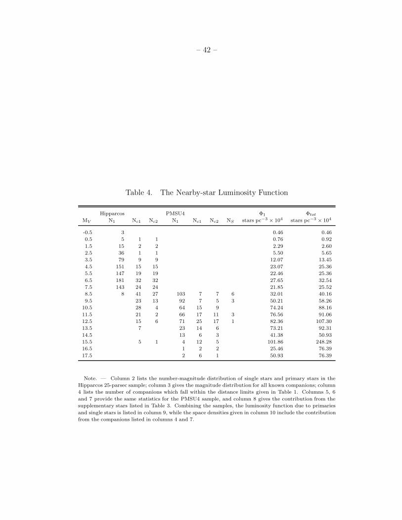
– 42 –

Table 4. The Nearby-star Luminosity Function

Hipparcos PMSU4 Φ1 Φtot

MV N1 Nc1 Nc2 N1 Nc1 Nc2 NS stars pc−3 × 104 stars pc−3 × 104

-0.5 3 0.46 0.46

0.5 5 1 1 0.76 0.92

1.5 15 2 2 2.29 2.60

2.5 36 1 1 5.50 5.65

3.5 79 9 9 12.07 13.45

4.5 151 15 15 23.07 25.36

5.5 147 19 19 22.46 25.36

6.5 181 32 32 27.65 32.54

7.5 143 24 24 21.85 25.52

8.5 8 41 27 103 7 7 6 32.01 40.16

9.5 23 13 92 7 5 3 50.21 58.26

10.5 28 4 64 15 9 74.24 88.16

11.5 21 2 66 17 11 3 76.56 91.06

12.5 15 6 71 25 17 1 82.36 107.30

13.5 7 23 14 6 73.21 92.31

14.5 13 6 3 41.38 50.93

15.5 5 1 4 12 5 101.86 248.28

16.5 1 2 2 25.46 76.39

17.5 2 6 1 50.93 76.39

Note. — Column 2 lists the number-magnitude distribution of single stars and primary stars in the

Hipparcos 25-parsec sample; column 3 gives the magnitude distribution for all known companions; column

4 lists the number of companions which fall within the distance limits given in Table 1. Columns 5, 6

and 7 provide the same statistics for the PMSU4 sample, and column 8 gives the contribution from the

supplementary stars listed in Table 3. Combining the samples, the luminosity function due to primaries

and single stars is listed in column 9, while the space densities given in column 10 include the contribution

from the companions listed in columns 4 and 7.

– 43 –

Table 5. Kinematics of nearby Stars

Sample 〈U〉 〈V 〉 〈W 〉 σU σV σW Comment

kms−1 kms−1 kms−1 kms−1 kms−1 kms−1

VC2 dM+dMe 436 -9.7 -22.4 -8.9 37.9 26.1 20.5 unweighted

42.1 32.9 32.2 |W | weighted

34 18 16 core

VC2 dMe 83 -15.4 -16.5 -10.1 25.0 21.1 17.8 unweighted

33.6 44.6 36.1 |W | weighted

12 11 11 core

Hipparcos MV < 4 137 -7.8 -10.0 -8.9 27.4 14.2 14.2 unweighted

29.4 15.4 21.8 |W | weighted

35 18 16 core

Hipparcos MV ≥ 4 532 -12.7 -22.8 -6.5 39.9 27.9 19.1 unweighted

45.2 33.4 29.2 |W | weighted

26 14 10 core

Note. — Unweighted: σ = Σ((xi − x)/n)

|W | Weighted: weighted using Wielen’s prescription (see text)

core: linear fit to central regions of probability distributions (Figure 16).

– 44 –

Figure Captions

Fig. 1.— A comparison between distance determinations pre- and post-Hipparcos. The

upper panel plots the difference, ∆d = dPMSU4 − dPMSU1, for the 1684 M dwarfs. The lower

panel shows the effect on the original VC sample, plotting the revised distances and absolute

magnitudes in comparison to the PMSU1 distance limits. 71 of 499 systems fall outwith the

formal sampling volume.

Fig. 2.— The run of density with increasimg distance for pCNS3 M dwarfs as a function

of absolute magnitude. The dotted vertical lines mark the distance limits for the volume-

complete sample; the dashed vertical line for MV =9.5 marks the value adopted in Paper I.

Fig. 3.— The distribution of the VC2 systems on the celestial sphere, as a function of both

equatorial and Galactic co-ordinates. The solid line indicates the −30◦ limit in both cases.

Fig. 4.— Comparison between the properties of the full VC2 sample and the subset of

stars identified in the Vyssotsky and Upgren objective prism surveys. The upper panels

plot the distribution as a function of distance: the left-hand panel shows the differential

number distribution, with the full sample plotted as a solid line and the spectroscopically-

identified subset as a dotted line; the right-hand panel shows the fractional contribution

from the spectroscopically-selected sample. The predominant contribution of the latter at

larger distances is clearly illustrated. The lower panels plot the differential distribution as a

function of tangential velocity, with the right-hand panel plotting the fractional contribution

from the spectroscopically-selected sample. The horizontal dotted line in the latter panel

indicates the fractional contribution of the latter stars to the full sample.

Fig. 5.— The (MV , (B-V)) colour-magnitude diagram for Hipparcos stars with π > 40 mas.

The four subdwarfs discussed in the text are plotted as solid triangles, while stars identified

as giants or subgiants are plotted as solid points.

Fig. 6.— The (MV , (B-V)) colour-magnitude diagram after adjusting magnitudes of close

binary systems to allow for the contribution from fainter components. Solid squares mark

stars in our 25-parsec sample: note that several fall below MV = 8 after correction for

binarity. Other symbols have the same meaning as in Figure 5.

Fig. 7.— The run of density with distance for main-sequence stars with 4 < MV < 8. The

initial point marks the mean density within 16 parsecs for each absolute magnitude interval;

subsequent points plot the density within annuli from 16 to 18, 18 to 20, 20 to 22 and 22 to 25

parsecs. There is no evidence for a significant downturn with increasing distance, indicating

– 45 –

a high degree of completeness in the sample.

Fig. 8.— The luminosity function for nearby stars, derived by combining data for the

Hipparcos 25-parsec sample and the PMSU sample. Data for single stars and primaries

are plotted as solid triangles; the open circles plot the space densities once the appropriate

companions are included, with the errorbars reflecting Poisson uncertainties. The solid

histogram plots Φ(MV ) from Wielen, Jahreiß & Kruger (1983).

Fig. 9.— The Duquennoy & Mayor G-dwarf sample: the lower figure compares the paral-

laxes listed in the CNS2 catalogue against the Hipparcos data; the upper figure plots the

distribution of the stars in the (MV , (B-V)) plane. Single stars are plotted as solid triangles,

binaries as open circles. The photometry of the latter stars has been corrected to exclude

contributions from secondary components.

Fig. 10.— The nearby star luminosity function, adjusted to include the contribution from

“missing” binary components. The symbols have the same meaning as in Figure 8. As

discussed in the text, we have doubled the contribution from known companions to the

Hipparcos 25-parsec sample.

Fig. 11.— The (MV , mass) relation for main-sequence stars: solid points and open circles

plot data for primary and secondary stars, respectively, from Andersen’s compilation of

eclipsing binaries; solid triangles plot data for lower main-sequence binaries from Segransan

et al. (2000). The five-point star marks the Sun. In the left-hand panel, the long-dashed line

shows the empirical fit to the upper main-sequence stars given in the text, the dotted line

plots the (MV , mass) relation derived by Delfosse et al. (2000) and the solid line shows the

three-component fit from Henry et al. (1993). Ther right-hand panel compares the former

two relations against the KTG semi-empirical relation (solid line).

Fig. 12.— The stellar mass function for the Solar Neighbourhood. The uppermost panel

shows the results of applying the mass-luminosity relation to the dataset used to derive

Φ(MV )) plotted in Figure 8, with the dotted histogram outlining the contribution from

single stars and primary stars in binary systems; the middle panel shows ξ(M) when double

weight is given to the Hipparos 25-parsec secondaries; the lowest panel shows ξ(M) for the

northern 8-parsec sample (Reid et al., 1999). In each case, the dashed lines plot the best-fit

power-law (see text).

Fig. 13.— A comparison between the present-day mass function derived using the empirical

mass-MV calibration (upper panel) and the KTG semi-empirical calibration (lower panel).

The latter includes the empirical eclipsing-binary relation for MV < 3.5. As in Figure 12, the

– 46 –

dotted histogram plots results for single stars/primaries. The main differences lie at near-

solar masses, with the semi-empirical calibration showing a steepening at ∼ 0.7M� rather

than ∼ 1M|odot.

Fig. 14.— The initial mass function: the upper panel shows results based on the empirical

mass-MV relation; the lower plots results using the KTG semi-empirical relation at MV > 3.5.

The units on the ordinate are surface density, with an arbitrary normalisation. The dashed

lines mark the power-law representations described in the text. The solid line and dotted

line plot log-normal functions, with the former plotting the best-fit function (see text) and

the latter, the original Millar-Scalo function with C1=1.15.

Fig. 15.— (U, V, W) diagrams for the VC2 (right-hand panels) and Hipparcos 25-parsec

(left-hand panels) datasets. Solid points mark dMe dwarfs in the VC2 sample and Hipparcos

stars with MV < 4.0, respectively.

Fig. 16.— Probability plots for (U, V, W) velocity distributions. The solid line plots data

for the full VC2 sample; the long-dashed lines outline data for the 83 dmE dwarfs in the VC2

sample; the dotted lines plot the distributions of the Hipparcos faint (MV > 4) sample; and

the short-dashed lines plot the bright (MV ≤ 4) Hipparcos dataset. The similarity between

the full VC2 and faint Hipparcos datasets is clear.

Fig. 17.— Two-component fits to probability plots of the W velocity distribution of the

PMSU VC2 M dwarf sample (upper plot) and the Hipparcos faint-star sample (lower plot).

In both cases, the observations are plotted as a solid line and the low-velocity component is

modelled with σW = 16 km s−1 ; the tabulated velocity distributions and relative normali-

sations refer to the higher-velocity component.

Fig. 18.— The uppermost panel plots the CaH2/TiO5 distribution of the VC2 M dwarfs

(squares), intermediate subdwarfs (sdM - triangles), and extreme subdwarf (esdM - open

circles). The solid lines are polynomial relations matched to the first two datasets. The

middle panel plots the CaH2 residuals for the VC2 dwarfs as a function of W velocity; the

lower panel plots those residuals normalised to the offset between the mean M dwarf and sdM

relations. Neither of the residual plots show evidence for a systematics trend with velocity.

– 47 –

Fig. 1.— A comparison between distance determinations pre- and post-Hipparcos. The

upper panel plots the difference, ∆d = dPMSU4 − dPMSU1, for the 1684 M dwarfs. The lower

panel shows the effect on the original VC sample, plotting the revised distances and absolute

magnitudes in comparison to the PMSU1 distance limits. 71 of 499 systems fall outwith the

formal sampling volume.

– 48 –

Fig. 2.— The run of density with increasimg distance for pCNS3 M dwarfs as a function

of absolute magnitude. The dotted vertical lines mark the distance limits for the volume-

complete sample; the dashed vertical line for MV =9.5 marks the value adopted in Paper

I.

– 49 –

RA

Galactic longitude

Fig. 3.— The distribution of the VC2 systems on the celestial sphere, as a function of both

equatorial and Galactic co-ordinates. The solid line indicates the −30◦ limit in both cases.

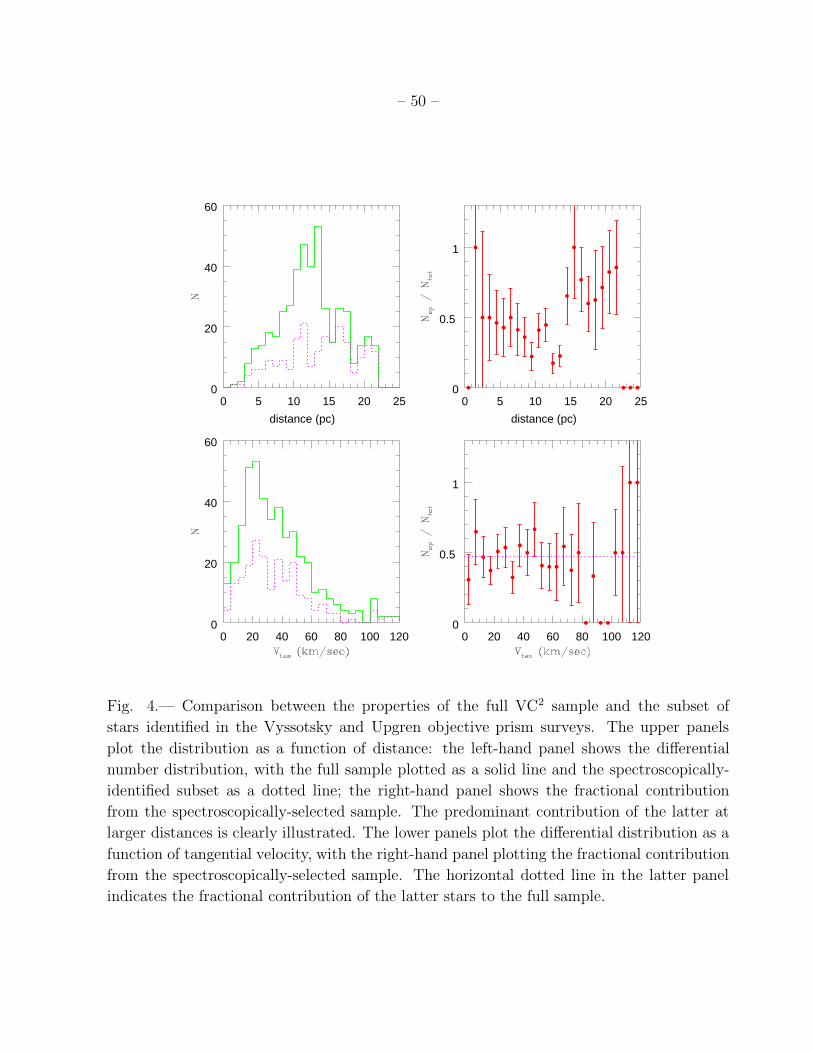
– 50 –

0 5 10 15 20 250

20

40

60

distance (pc)

0 5 10 15 20 250

0.5

1

distance (pc)

0 20 40 60 80 100 1200

20

40

60

0 20 40 60 80 100 1200

0.5

1

Fig. 4.— Comparison between the properties of the full VC2 sample and the subset of

stars identified in the Vyssotsky and Upgren objective prism surveys. The upper panels

plot the distribution as a function of distance: the left-hand panel shows the differential

number distribution, with the full sample plotted as a solid line and the spectroscopically-

identified subset as a dotted line; the right-hand panel shows the fractional contribution

from the spectroscopically-selected sample. The predominant contribution of the latter at

larger distances is clearly illustrated. The lower panels plot the differential distribution as a

function of tangential velocity, with the right-hand panel plotting the fractional contribution

from the spectroscopically-selected sample. The horizontal dotted line in the latter panel

indicates the fractional contribution of the latter stars to the full sample.

– 51 –

Fig. 5.— The (MV , (B-V)) colour-magnitude diagram for Hipparcos stars with π > 40 mas.

The four subdwarfs discussed in the text are plotted as solid triangles, while stars identified

as giants or subgiants are plotted as solid points.

– 52 –

Fig. 6.— The (MV , (B-V)) colour-magnitude diagram after adjusting magnitudes of close

binary systems to allow for the contribution from fainter components. Solid squares mark

stars in our 25-parsec sample: note that several fall below MV = 8 after correction for

binarity. Other symbols have the same meaning as in Figure 5.

– 53 –

14 16 18 20 22 24 260

0.002

0.004

Distance (pc)

14 16 18 20 22 24 260

0.002

0.004

Distance (pc)

14 16 18 20 22 24 260

0.002

0.004

Distance (pc)

14 16 18 20 22 24 260

0.002

0.004

Distance (pc)

Fig. 7.— The run of density with distance for main-sequence stars with 4 < MV < 8. The

initial point marks the mean density within 16 parsecs for each absolute magnitude interval;

subsequent points plot the density within annuli from 16 to 18, 18 to 20, 20 to 22 and 22 to 25

parsecs. There is no evidence for a significant downturn with increasing distance, indicating

a high degree of completeness in the sample.

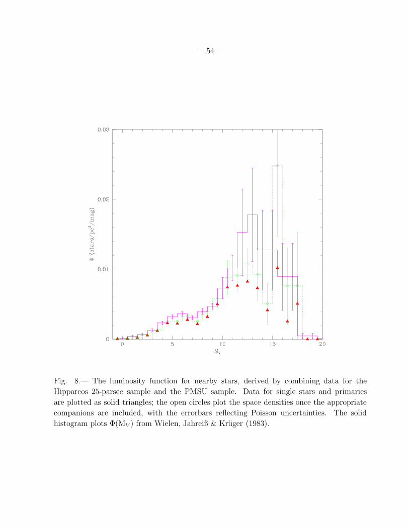
– 54 –

Fig. 8.— The luminosity function for nearby stars, derived by combining data for the

Hipparcos 25-parsec sample and the PMSU sample. Data for single stars and primaries

are plotted as solid triangles; the open circles plot the space densities once the appropriate

companions are included, with the errorbars reflecting Poisson uncertainties. The solid

histogram plots Φ(MV ) from Wielen, Jahreiß & Kruger (1983).

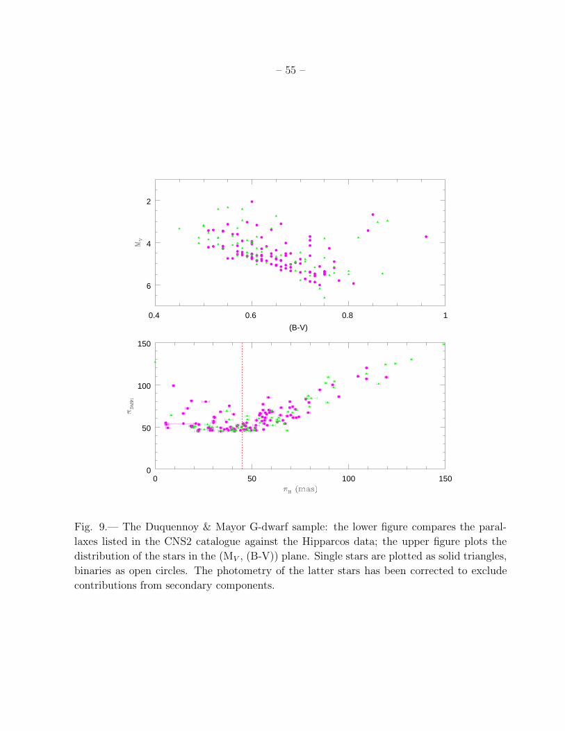
– 55 –

0.4 0.6 0.8 1

6

4

2

(B-V)

0 50 100 1500

50

100

150

Fig. 9.— The Duquennoy & Mayor G-dwarf sample: the lower figure compares the paral-

laxes listed in the CNS2 catalogue against the Hipparcos data; the upper figure plots the

distribution of the stars in the (MV , (B-V)) plane. Single stars are plotted as solid triangles,

binaries as open circles. The photometry of the latter stars has been corrected to exclude

contributions from secondary components.

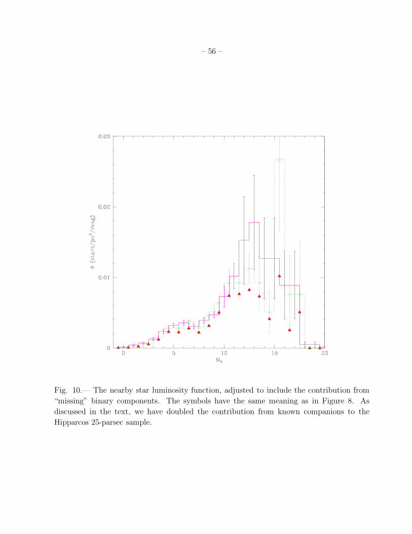
– 56 –

Fig. 10.— The nearby star luminosity function, adjusted to include the contribution from

“missing” binary components. The symbols have the same meaning as in Figure 8. As

discussed in the text, we have doubled the contribution from known companions to the

Hipparcos 25-parsec sample.

– 57 –

-5 0 5 10 15

-1

-0.5

0

0.5

1

Fig. 11.— The (MV , mass) relation for main-sequence stars: solid points and open circles

plot data for primary and secondary stars, respectively, from Andersen’s compilation of

eclipsing binaries; solid triangles plot data for lower main-sequence binaries from Segresan et

al. (2000). The five-point star marks the Sun. In the left-hand panel, the long-dashed line

shows the empirical fit to the upper main-sequence stars given in the text, the dotted line

plots the (MV , mass) relation derived by Delfosse et al. (2000) and the solid line shows the

three-component fit from Henry et al. (1993). Ther right-hand panel compares the former

two relations against the KTG semi-empirical relation (solid line).

– 58 –

-1 -0.5 0 0.5 1-5

-4

-3

-2

-1

log(mass)

Hipparcos + PMSU

-1 -0.5 0 0.5 1-5

-4

-3

-2

-1

log(mass)

8 pc. sample

-1 -0.5 0 0.5 1-5

-4

-3

-2

-1

log(mass)

Hipparcos + PMSU

2 x binaries

Fig. 12.— The stellar mass function for the Solar Neighbourhood. The uppermost panel

shows the results of applying the mass-luminosity relation to the dataset used to derive

Φ(MV )) plotted in Figure 8, with the dotted histogram outlining the contribution from

single stars and primary stars in binary systems; the middle panel shows ξ(M) when double

weight is given to the Hipparos 25-parsec secondaries; the lowest panel shows ξ(M) for the

northern 8-parsec sample (Reid et al., 1999). In each case, the dashed lines plot the best-fit

power-law (see text).

– 59 –

-1 -0.5 0 0.5 1-5

-4

-3

-2

-1

log (mass)

Andersen+KTG

-1 -0.5 0 0.5 1-5

-4

-3

-2

-1

log(mass)

Andersen + D00

Fig. 13.— A comparison betweenthe present-day mass function derived using the empirical

mass-MV calibration (upper panel) and the KTG semi-empirical calibration (lower panel).

The latter includes the empirical eclipsing-binary relation for MV < 3.5. As in Figure 12, the

dotted histogram plots results for single stars/primaries. The main differences lie at near-

solar masses, with the semi-empirical calibration showing a steepening at ∼ 0.7M� rather

than ∼ 1M|odot.

– 60 –

-1 -0.5 0 0.5 1

-1

0

1

log(mass)

Andersen+D00

IMF

-1 -0.5 0 0.5 1

-1

0

1

log(mass)

Andersen+KTG

IMF

Fig. 14.— The initial mass function: the upper panel shows results based on the empirical

mass-MV relation; the lower plots results using the KTG semi-empirical relation at MV > 3.5.

The units on the ordinate are surface density, with an arbitrary normalisation. The dashed

lines mark the power-law representations described in the text. The solid line and dotted

line plot log-normal functions, with the former plotting the best-fit function (see text) and

the latter, the original Millar-Scalo function with C1=1.15.

– 61 –

-150 -100 -50 0 50-100

-50

0

50

100

V km/sec

-150 -100 -50 0 50-100

-50

0

50

100

V km/sec

-150 -100 -50 0 50-100

-50

0

50

100

V km/sec

-150 -100 -50 0 50-100

-50

0

50

100

V km/sec

Fig. 15.— (U, V, W) diagrams for the VC2 (right-hand panels) and Hipparcos 25-parsec

(left-hand panels) datasets. Solid points mark dMe dwarfs in the VC2 sample and Hipparcos

stars with MV < 4.0, respectively.

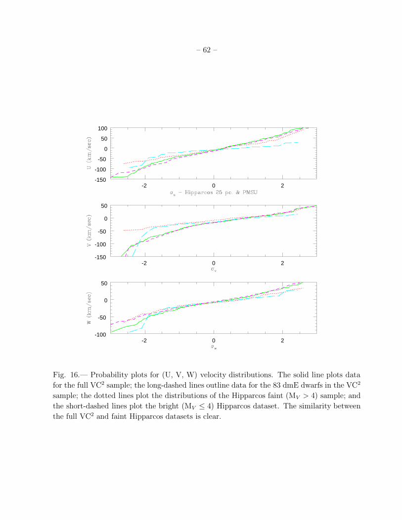
– 62 –

-2 0 2-150

-100

-50

0

50

100

-2 0 2-150

-100

-50

0

50

-2 0 2-100

-50

0

50

Fig. 16.— Probability plots for (U, V, W) velocity distributions. The solid line plots data

for the full VC2 sample; the long-dashed lines outline data for the 83 dmE dwarfs in the VC2

sample; the dotted lines plot the distributions of the Hipparcos faint (MV > 4) sample; and

the short-dashed lines plot the bright (MV ≤ 4) Hipparcos dataset. The similarity between

the full VC2 and faint Hipparcos datasets is clear.

– 63 –

-4 -2 0 2 4

-100

-50

0

50

-4 -2 0 2 4

-100

-50

0

50

Fig. 17.— Two-component fits to probability plots of the W velocity distribution of the

PMSU VC2 M dwarf sample (upper plot) and the Hipparcos faint-star sample (lower plot).

In both cases, the observations are plotted as a solid line and the low-velocity component is

modelled with σW = 16 km s−1 ; the tabulated velocity distributions and relative normali-

sations refer to the higher-velocity component.

– 64 –

Fig. 18.— The uppermost panel plots the CaH2/TiO5 distribution of the VC2 M dwarfs

(squares), intermediate subdwarfs (sdM - triangles), and extreme subdwarf (esdM - open

circles). The solid lines are polynomial relations matched to the first two datasets. The

middle panel plots the CaH2 residuals for the VC2 dwarfs as a function of W velocity; the

lower panel plots those residuals normalised to the offset between the mean M dwarf and sdM

relations. Neither of the residual plots show evidence for a systematics trend with velocity.