The Political Economy of FinancialInnovation: Evidence from Local

Governments

Christophe Perignon ∗ Boris Vallee †‡

First Draft: July 30, 2011This Draft: December 5, 2015

Abstract

We present an empirical investigation of the political economy of financial in-novation. Our findings show that financial innovation can amplify principal-agentproblems within the political system. The adoption of structured loans, a high-risk type of borrowing for local governments, is more frequent for politicians fromhighly indebted local government, from politically contested areas, and during po-litical campaigns. We also show that using structured loans helps incumbents getre-elected, and allows them to maintain lower taxes. Conversely, structured loanusage is hard to empirically reconcile with politicians’ ex post claim that they donot understand the transactions.

Keywords : Financial innovation, Political Economy, Principal-agent problem, Structured

debt

JEL codes: P16, H74, G11, G32

∗HEC Paris - Email: perignon@hec.fr. Address: Finance Department, HEC Paris, 1, rue de laLiberation, 78350 Jouy-en-Josas, France - Phone: +33 139 67 94 11

†Harvard Business School - Email: bvallee@hbs.edu. Address: Finance Department, HarvardBusiness School, Baker Library 245, Boston MA02163 - Phone: 617-496-4604 (corresponding author)

‡This article is based on a chapter of Boris Vallee’s PhD dissertation at HEC Paris. We are gratefulto Malcolm Baker, Marianne Bertrand, Claire Celerier, Jonathan Dark, Francois Derrien, Dirk Jenter,Laurent Fresard, Jeffry Frieden, Thierry Foucault, Robin Greenwood, Benjamin Hebert (NBER discus-sant), Ulrich Hege, Jose Liberti (EFA discussant), Steven Ongena, Clemens Otto, Stavros Panageas,Guillaume Plantin, Josh Rauh, Jean-Charles Rochet, Paola Sapienza, Antoinette Schoar, Amit Seru,Andrew Siegel, Jerome Taillard, David Thesmar, Philip Valta, James Vickery (WFA discussant), partic-ipants at the 2015 NBER Corporate Finance meeting, the 2012 WFA meeting, the 2013 EFA meeting,the 2015 Brandeis-Boston Fed Municipal Finance Conference, and seminar participants at the Banquede France, HEC Paris, INSEAD, and University of Zurich, for their helpful comments and suggestions.We also thank the French Ministry of the Interior, and the Centre de Donnees Socio-Politiques (CDSP)for providing some of the data. All errors are ours only.

1

“We are playing the dollar against the Swiss franc until 2042.”

Cedric Grail, CEO of City of Saint Etienne, France (Business Week, 2010)

1 Introduction

The political economy of financial innovation arguably played an important role in the

recent financial crisis (Zingales, 2015). Politicians’ willingness to facilitate access to home-

ownership might have fueled the mortgage-backed securities market (Rajan, 2010). To

comply with Eurozone requirements, Greece entered into OTC swap transactions to hide

a significant part of its debt. The role of political incentives in the development of in-

novative financial products remains, however, largely debated and difficult to identify

empirically. The research question we address in this paper is whether financial inno-

vation amplifies principal-agent problems in the political system. Because voters and

politicians’ interests do not necessarily align, agency costs frequently emerge in the polit-

ical system. Innovative financial products might exacerbate these issues if they facilitate

politicians’ strategies.

To address this research question we exploit the recent development of an innovative

form of borrowing by local governments: structured loans.1 These loans have three

defining features: a long maturity, a fixed/low interest rate for the initial period of the

loan, and an adjustable rate that depends on the value of a given financial index (e.g.,

Libor, foreign exchange rate or swap rate spreads). When borrowing with the most

popular type of structured loan, the so-called Steepener, a local government pays an

interest rate such as:

Year 1-5: 2%

Year 6-20: 2% if 10Y Swap Rate - 2Y Swap Rate ≤ 1%

10% - 8 × (10Y Swap Rate - 2Y Swap Rate) otherwise

These loans shift a large share of the borrower’s immediate cost of debt to certain

states of nature in the future, allowing budget relief for an initial period, which typi-

cally matches the politician’s current term of office. Local government structured loans

1These loans embed derivatives, such as options. Designing asset or liability side financial productsthat embed options on a range of underlying financial assets is an innovation from the early 2000s.

2

represent an ideal laboratory for studying the political economy of financial innovation

for three reasons: structured loans offer great flexibility to the borrowers in terms of

cash-flow distribution across time and states of nature; these transactions are typically

undisclosed to voters; and finally the large number of local governments using structured

loans in France allow for a large sample empirical analysis.

The local government structured loan phenomenon has been observed in Europe, Asia,

and, to a lesser extent, the US. In France alone, outstanding products represent more

than EUR30 billion and bear unrealized losses exceeding EUR10 billion, or 0.5% of GDP

(Cour des Comptes, 2011). During the recent financial crisis, as volatility spiked, the

interest costs of structured loan users increased to double digit levels and may remain

high for the remainder of their lifetimes.2

Using proprietary data from France, we provide empirical evidence consistent with

politicians strategically using risky innovative financial products for their own interest.

First, we document the extent to which politicians have been implementing these risky

transactions: structured loans account for more than 20% of outstanding local government

debt, and more than 72% of the 300 largest local governments use structured loans.

Among these structured loans, 40% bear a significantly high level of risk.

Second, we show that the propensity, size, and timing of these transactions vary ac-

cording to politicians’ incentives. A cross-section of our data illustrates how politicians

from highly indebted local governments are significantly more likely to turn to this type of

loan, evidencing a higher incentive to hide the actual cost of debt. We provide additional

evidence suggesting a causal link between the level of indebtedness and the local govern-

ment’s propensity to use structured debt by instrumenting the level of local government

debt with floods, an arguably exogenous source of expenditures. We also find that in-

cumbent politicians running in politically contested areas, as opposed to strongholds, are

more inclined to use structured loans, which is consistent with them shifting cash-flows in

the future to aid them in being re-elected in the short run. When comparing a treatment

group that confronts elections during our sample period (municipalities and counties),

to a control group that does not (regions, hospitals, and social housing entities), we find

that structured loan transactions are more frequent during the political campaign than

2For instance, the City of Saint-Etienne saw the annual interest rate charged to one of its major loansincreased from 4% to 24% in 2010, as the latter was indexed to the British pound/Swiss franc exchangerate (Business Week, 2010).

3

after the election.

Third, we explore the real effects of structured loan usage. By instrumenting the use

of structured loans with the distance to the closest branch of the leading bank, we find

that structured loan usage increases the likelihood for a politician to get re-elected. We

also provide evidence suggesting that politicians using structured loans maintain lower

local taxes, a political choice itself correlated with re-election.

Finally, our empirical evidence is hard to reconcile with other explanations for the

development of the market: banks exploiting a potential lack of financial sophistication

from politicians, and a hedging demand from local governments. First, controlling for

local government size, politicians whose profession requires higher education are more

inclined to use structured loans than politicians from a less educated background. Second,

revenues of local governments do not correlate with the exposure provided by structured

loans.

Our empirical analysis relies on two proprietary datasets that contain detailed infor-

mation on structured loan usage in France. Our first dataset contains the entire debt

portfolio for a sample of the 300 largest French local governments as of the end of 2007.

For each debt instrument, we observe the notional amount, maturity, type of product,

underlying financial index, and lender identity. Structured debt amounts to EUR10.4

billion for this sample, out of EUR52 billion total debt. Our second dataset includes all

of the structured transactions made by Dexia, the leading bank on the French market for

local government loans, between 2000 and 2009. This dataset provides loan-level infor-

mation, including the mark to market and transaction date. It also contains information

for more than 2,700 local governments (see Appendix A for more information on local

government types), for a total of EUR23.7 billion of outstanding structured loans. We

complement the second dataset with detailed accounting data, election results, list of

floods, mayor demographics, and GPS coordinates.

Our methodology relies mainly on probit regressions where the dependent variable

is an indicator of the use of structured loans. To strengthen identification, we comple-

ment these correlation specifications with two distinct instrumental variable analyses:

we instrument indebtedness with the occurrence of floods, the most widespread type

of natural catastrophe in France, and we instrument the propensity to use structured

loans with the distance to the closest branch of the main lender. We also implement a

4

difference-in-differences specification when analyzing the role of election timing.

Our paper relates to two streams of literature. First, our work complements studies

of the political economy of finance, including political agency problems (Besley and Case,

1995), political incentives and credit (Rajan, 2010), their influence on financial decisions

for local governments (Butler et al. (2009), Ang et al. (2014)), or on bank bailouts (Behn

et al., 2014). Aneja et al. (2015) show that politicians can use financial instruments as

a way to signal their commitment. Tightly related to our findings on election timing,

Dinc (2005) shows that government banks lend more in election years, while Bertrand

et al. (2007) document that politicians influence CEOs to avoid layoffs prior to elections.

Halling et al. (2014) document revenue transfers from government owned banks to local

governments. We also complement findings on the economic effects of political uncertainty

(Julio and Yook, 2012), with a public finance channel. Because structured loans allow

local governments to cosmetically reduce their immediate cost of debt, our work directly

relates to the off-balance sheet borrowing of local governments, mainly through pension

fund liabilities (Novy-Marx and Rauh, 2011). Our study also offers a non-bank set-up to

consider collective moral hazard (Farhi and Tirole, 2012).

Second, our paper contributes to the debate on the dark side of financial innovation

(Shiller, 2013; Simsek, 2013), its associated risks (Gennaioli et al., 2012), motives (Celerier

and Vallee, 2015), and effects (Rajan, 2006). Similar to the sophisticated mortgage

borrowers studied by Amromin et al. (2013), politicians may deliberately exploit certain

characteristics of innovative financial products to their own advantage, regardless of the

long-term risks they impose on the taxpayer.

Through the alternative explanations we consider, our work also builds on the finan-

cial literacy literature (Lusardi and Mitchell, 2011), and studies of hedging policies by

corporate firms (Baker et al., 2005).

The paper proceeds as follows. In Section 2, we provide background on the local gov-

ernment market for structured loans, and describe our datasets in Section 3. We develop

our hypotheses in Section 4, which we subsequently test in Section 5 for structured loan

usage, and in Section 6 for the effects of structured loan usage. We consider alternative

explanations in Section 7. We conclude our study in Section 8.

5

2 Market Background

This section provides some background information on the local government market for

structured loans, including a detailed structured product example, and classify structured

loans by their level of risk.3

2.1 Structured Loan Characteristics

In this study, a structured loan refers to a bank loan obtained by a local government,

in which the interest rate formula differs from either a constant fixed rate, or a floating

rate such as Libor + a spread (referred to as “standard loans” throughout this study).

Structured loans offer an initial period with a guaranteed low interest rate, which typically

lasts between two and seven years. In a subsequent period, the interest rate follows a

formula based on a given underlying financial index. The loan design embeds a sale

of options on this underlying financial index by the borrower, meaning that the local

government will pay a higher interest rate if the underlying reaches a certain threshold.4

In exchange, the borrower receives the option premium, which is subtracted from the

interest cost. As with any short position in options, the risk of the transaction increases

with its maturity, the volatility of the underlying index, the leverage in the interest rate

formula, and the cap level.5 Local governments are among the issuers that have the

longest debt maturity, typically ranging from 15 to 30 years, which is a prerequisite for

structuring products with several years of guaranteed low interest rates. There are three

main designs for obtaining a large option premium, thereby substantially decreasing the

initial interest rate. First, the structured loan can be indexed to a highly volatile index,

such as foreign exchange, which increases the likelihood that the threshold will be reached.

Second, the formula can be levered, as in the Steepener example in the introduction.

Third, the formula can rely on a carry-trade, for instance by creating a long position in

a high interest rate currency and a short one in a low interest rate currency.

Below is an example of a structured loan subscribed by the Rhone, the French county

3These institutional details rely on product term sheets, on the French Congress investigation into thestructured loan market (French National Assembly, 2011), and numerous discussions with professionalsfrom both buy and sell sides.

4See Appendix B for a typology of the structured loans.5Structured loans generally do not possess any cap feature, meaning that there is no ceiling to the

interest rates the borrower may face.

6

that comprises the city of Lyon. The loan has an eight-year initial period with a low

guaranteed interest rate of 1.75%, which is significantly lower than the interest rate on

an equivalent standard loan at the time of issuance (4.50%). In the subsequent period,

the loan offers a fixed rate that is conditioned on the EURCHF exchange rate. The loan

therefore generates a leveraged and uncapped exposure to CHF appreciation against EUR

for the remaining 17 years. At today’s levels (as of December 2015), the interest rate on

this loan is about 31%. Similar products with higher leverage or strikes result in some

local governments currently paying more than a 50% interest rate per year.

Amount: EUR 80 million

Trade Year: 2006

Loan Maturity: 2031

Year 2006-2013: 1.75%

Year 2014-2031: 1.75%+ Max(1.40/EURCHF(t)-1,0%)

As the equivalent fixed rate at the time of issuance was around 4.50%, the interest

rate formula can be rewritten as:

Year 2006-2013: 4.50% - 2.75%

Year 2014-2031: 4.50% - 2.75%+ Max(1.40/EURCHF(t)-1,0%)

This illustrates how the sale of an option on EURCHF during the years 2014-2031 provides

the local government with a yearly premium of 2.75%.

2.2 Impact on Financial Statements

Structured loans allow local governments to immediately reduce the cost of their debt in

their financial statements, and therefore provide an immediate budget relief. This relief

is certain for the period during which the interest rate is guaranteed, and extends to

the subsequent period subject to conditions. Local governments can budget this relief

and immediately adapt expenditures accordingly.6 Anecdotal evidence suggests that the

6An important aspect of French governmental accounting is that local governments are forbidden fromborrowing to balance their operating budget. Loan proceeds can only be used for investment purposes.However, the cost of debt is considered as an operating expense: structured loans are therefore a way ofbalancing the budget and relaxing the financial constraint in the short term.

7

guaranteed period is often designed to cover the remaining length of the local politician’s

mandate. The subsidy is repaid in the future in certain states of nature, namely, when the

options embedded in the derivative component of the loan end up in the money. Under

most governmental accounting standards, derivatives (either stand-alone swaps or those

embedded within structured loans) are not accounted for at fair value. In many countries,

including France, governmental accounting standards do not even require the disclosure

of derivatives transactions. Only the interests that are paid during the accounting year

must appear in financial statements, which makes it challenging for taxpayers to identify

the true cause behind a decrease in the cost of debt of a local government.

In the previous example, the product provides a 2.75% annual subsidy for seven years,

which is the difference between the rate on an equivalent standard loan and the one on

the structured loan. If the entire debt of the local government consists of this type of

financing, the cost of debt may therefore appear less than half of what it should be.

2.3 Supply Side Characteristics

The competitive landscape of the structured loan market in Europe consists of banks

specialized in local governments, such as Dexia or Depfa, and universal banks. Both

possess the necessary balance sheet, the local client portfolio, and the structuring exper-

tise. Though the market for structured loans is dominated by national players who have

historical relationships, some of the universal banks are active across several European

countries, such as Royal Bank of Scotland and Deutsche Bank.7

Anecdotal evidence suggests that structured loan transactions are highly profitable

for banks, with markups being significantly higher (around 5% of the loan notional) than

for standard loans. This level of profitability is however lower than the one of retail

structured products, which developed in the same period.8

Despite the long term credit exposure they generate, and the inexistence of CDS

to hedge it, banks do not ask local government to post collateral on these transactions.

Collateral requirements, typically in place with corporate clients, would hinder structured

transactions for local governments, as margin calls would be both costly to manage and

7Both these banks are active in France. Goldman Sachs and Royal Bank of Canada also entered themarket, however they never gained a significant market share.

8Although the magnitude of absolute markups is comparable (Celerier and Vallee, 2015), retail prod-ucts maturity is much shorter, around five years on average, versus 15 for structured loans.

8

visible to voters.

2.4 Risk Classification

As many local governments are currently paying double-digit interest rates on their struc-

tured loans, the press has labeled them “toxic”. Some structured loans indeed present

unusually-high levels of risk, as local governments may pay significantly more in interest

than the amount borrowed. In this study, we rely on the classification established by the

French Government following the first litigations, the Gissler scale, to measure the risk

of structured loans. Although they all rely on the same mechanism (an implicit sale of

options, the premium of which is subtracted from the initial interest rate), structured

loans exhibit diverse risk profiles, which also correspond to different magnitudes of short-

term budget relief: the riskier the product, the lower the interest rate during the initial

subsidy period, and/or the longer this period. The Gissler scale ranks structured loans

according to their risk profile. For more details regarding the different types of structured

loan, and the Gissler scale, see Appendix B.

We classify a structured product as high-risk if it is equal or higher than 3 on the

Gissler scale. Given this definition, loans that are indexed to the interest rate curve slope,

foreign interest rates, or to a foreign exchange rate are classified as high-risk. Products

that are linked to domestic interest rates or inflation are not considered high-risk. High-

risk products are a more recent development of the market.

This classification is based on loan characteristics at inception and is independent from

the market conditions that prevail during the life of the product. A high-risk product may

have offered a low interest rate level to its user ex post ; nevertheless, the borrower entered

into a transaction that would have created massive losses had the market situation been

reversed. Structured products that are not classified as high-risk still bear significantly

more risk than standard financing, as their nonlinear payoffs can trigger sudden increases

in the cost of debt.

2.5 Post-Crisis Developments

The financial crisis led to a spike of volatility in all financial markets, which led to large

unrealized losses on structured loans, and in many cases caused the interest rates to

9

jump to double-digit levels. Starting in 2010, local governments have been unwilling to

pay these high interest rates, and have been suing banks for mis-advice and questioning

whether these transactions are legal in the first place. Local governments across Europe

attempted to obtain the cancellation of the structured loans, especially the high-risk ones,

or to negotiate an exit at better terms.

In France, court outcomes have been mixed, but initially led to the cancellation of

some structured loans. This decision was later repelled by the Higher Court of Justice

in France, and a retroactive law was introduced to ensure the legality of all existing

transactions. A partial government bailout was implemented in 2014, in the form of

a 50% participation of the central government in unwinding costs. This government

subsidy is financed half by a new tax on banks’ systemic risk contributions. The amount

allocated to this purpose has been increased from EUR1.5bn to EUR3bn at the beginning

of 2015, following the change in the Swiss National Bank policy that led to severe losses on

products indexed to the EURCHF exchange rate. The French government faces a trade-

off between having only local taxpayers pay for the structured loan losses, or sharing the

cost nationwide. Moreover, the main player in the market, Dexia, has been nationalized

during the financial crisis.9 Therefore, cancelling all local governments’ unrealized losses

would be extremely costly for the French central government, which may have played a

role in implementing the new legislation.

3 Data

Our analysis relies on two proprietary datasets that contain a wealth of information on

local governments’ structured loans, traditionally undisclosed to voters.

Our analysis requires information on the composition – and not only the total amount

– of the debt portfolio for a sample of local governments. We obtain this information

from two separate sources. The first dataset contains the entire debt portfolio for almost

all of the 300 largest French local governments (Dataset A) as of December 31, 2007.

The second set includes loan level data on all the outstanding structured transactions in

France of Dexia, the leading bank on the market (Dataset B) as of December 31, 2009.

9Dexia’s bailout did not stem from its local government operations, which remained solvent throughoutthe crisis, but from losses at its US subsidiary, the monoliner FSA, and from a large loan made to troubledDEPFA bank.

10

We complement these two datasets with local governments’ detailed financial statements,

the list of floods in France, results of municipal elections in France, GPS data to measure

distances, and demographic characteristics of mayors.

3.1 Local Government Level Debt Data (Dataset A)

Our first dataset, which covers 293 French local governments, comes from a leading

European financial consulting firm for local governments. This dataset contains the entire

debt portfolio, broken down by type of debt, for nearly all the largest local governments:

French regions (25 out of 27) and French Counties (96 out of 100) as well as the largest

cities (96) and intercity associations (76). Collectively, these local governments have a

total debt of EUR52 billion, or 38.2% of the total debt of all French local governments,

which includes EUR10 billion of structured debt, or a third of the total outstanding

amount in France as estimated by the French Congress. Panel A of Table 1 provides

summary statistics on the debt profile of the local governments from the sample.

[Insert Table 1 here]

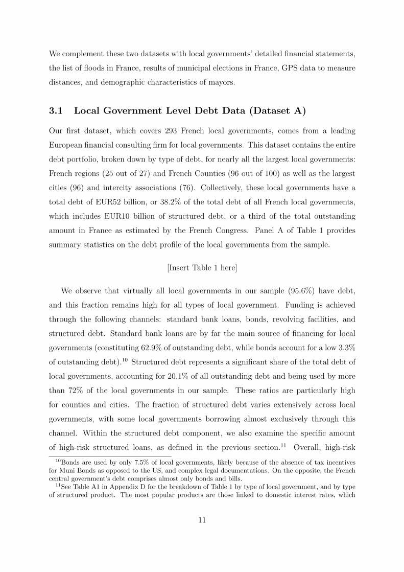
We observe that virtually all local governments in our sample (95.6%) have debt,

and this fraction remains high for all types of local government. Funding is achieved

through the following channels: standard bank loans, bonds, revolving facilities, and

structured debt. Standard bank loans are by far the main source of financing for local

governments (constituting 62.9% of outstanding debt, while bonds account for a low 3.3%

of outstanding debt).10 Structured debt represents a significant share of the total debt of

local governments, accounting for 20.1% of all outstanding debt and being used by more

than 72% of the local governments in our sample. These ratios are particularly high

for counties and cities. The fraction of structured debt varies extensively across local

governments, with some local governments borrowing almost exclusively through this

channel. Within the structured debt component, we also examine the specific amount

of high-risk structured loans, as defined in the previous section.11 Overall, high-risk

10Bonds are used by only 7.5% of local governments, likely because of the absence of tax incentivesfor Muni Bonds as opposed to the US, and complex legal documentations. On the opposite, the Frenchcentral government’s debt comprises almost only bonds and bills.

11See Table A1 in Appendix D for the breakdown of Table 1 by type of local government, and by typeof structured product. The most popular products are those linked to domestic interest rates, which

11

structured loans represent 8.4% of total debt in our sample, and are used by 43% of the

local governments. Again, there is significant heterogeneity among local governments in

their use, with some governments having up to 71.7% of their total debt consisting of

high-risk structured loans.

3.2 Loan Level Data on Structured Transactions (Dataset B)

Our second dataset contains loan level data for all structured loan transactions imple-

mented with Dexia, the largest lender in this market, between 2000 and 2009. This

second dataset is almost ten times larger than the first, as Dexia represents more than

60% of the market for public sector-structured loans (French National Assembly, 2011).

The French newspaper Liberation posted these confidential risk-management data on its

website following an internal leak from the bank. This dataset contains 2,741 different

public sector entities: 16 regions (vs. 25 in Dataset A); 66 counties (vs. 96); 539 inter-

cities (vs. 76); 1,588 municipalities (vs. 96); 288 hospitals (vs. zero); 115 social housing

entities (vs. zero); and 129 other borrowers, including airports, harbors, chambers of

commerce, healthcare cooperatives, public-private joint ventures, schools, research insti-

tutes, nursing homes, fair organizers, and charities. The local governments in our sample

vary significantly in terms of size; for instance, 37 cities have fewer than 1,000 inhabitants,

and 29 cities have more than 100,000 inhabitants.12

Panel B of Table 1 provides summary statistics for this dataset.13 By construction,

every local government in this sample uses at least one structured loan, for a total amount

of EUR23 billion, or more than two thirds of the total amount estimated by the French

National Assembly. In this sample, more than EUR13 billion of structured loans are

considered high-risk under our classification. The average amount of structured loan per

local government is much lower than in the previous dataset, mostly due to the larger

sample that includes many entities of small size. The average number of structured

transactions is approximately two, but 163 entities have more than five structured loans

account for nearly half of the outstanding structured debt (47.7%). Other underlying indices (sorted bydecreasing popularity) include the interest rate curve slope (26.8%), foreign exchange (14.8%), inflation(3.4%), and foreign interest rates (2.4%).

12There are more than 36,000 municipalities in France, the majority having less than 500 inhabitants.13The number of observations is lower for total debt because Dataset B has to be matched with

accounting data.

12

in their debt portfolio.14

The data also include information on trade inception dates, allowing us to build a panel

to conduct time-series analysis.15 The aggregated numbers of transactions per semester

are plotted in Figure 1. We observe the rapid development of the market followed by a

sharp contraction after 2007. The latter was exacerbated by media coverage of distressed

local governments and by Dexia’s own difficulties in the last quarter of 2008. This figure

also evidences the evolution of the composition of the transactions implemented: high-

risk structured loans, as defined in the previous section, become more and more prevalent

over time.

[Insert Figure 1 here]

3.3 Complementary Datasets

We complement the previous structured loan data with five types of data: detailed ac-

counting data, election results, mayor demographics, the list of floods in France, and

GPS coordinates.16 The accounting data, provided by the French Ministry of the Inte-

rior, include the highest level of detail possible for balance sheet and income statement, at

an annual frequency for the period 2002-2012. These accounting data are under French

governmental accounting standards. The dataset on election results, provided by the

Center for Socio-Political Data (CDSP), includes the votes obtained by each political

party during French municipal elections going back up to 1983. The sample covers all

municipalities with more than 9,000 inhabitants. The third complementary dataset in-

cludes information on age, gender, political affiliation, and professional occupation for all

the mayors in France since 2001. These data are collected by the French Ministry of the

Interior and constitute the Registre National des Elus. We collect the list of floods, by

municipality, from the Ministerial Decrees on natural catastrophes in France.17 Floods

14The data also contain information on the mark-to-market of transactions as of the end of 2009. Themark-to-market corresponds to the market value of unwinding the derivative position, and is negativefor local governments in 92% of the cases.

15For this purpose, we assume no loan repayments by local governments, and a linear amortizationschedule for these loans. Both these assumptions come from discussions with practitioners, who informedus that loan early repayments are extremely rare, and that the majority of the structured loans followthis type of profile.

16Dataset A being anonymized, we only match these data to dataset B.17The complete list of floods is available at: http://macommune.prim.net/gaspar.

13

are the most frequent type of natural disaster in France. These data are cleanly matched

with the other datasets using municipalities unique identifier, INSEE code. GPS coordi-

nates for municipalities and Dexia branches allow us to calculate distances as the crow

flies for the purpose of our instrumental variable analysis.

4 Hypotheses

We build on the theory of incentives, more specifically principal-agent models, to structure

our empirical analysis of the political economy of financial innovation.

The principal-agent model (Jensen and Meckling, 1976) is one of the most influential

frameworks in both economics and political science. Because voters’ (the principal) and

politicians’ (the agent) interests do not necessarily align, agency costs frequently emerge

in the political system. As the sovereign debt crisis in Europe illustrates, politicians

may focus on getting re-elected at the expense of implementing sound budget decisions.

Agency problems are amplified in specific environments, for instance when agent actions

are not observable by the principal, or when the cost of current decisions can be shifted

in the future. A financial innovation may be designed to fulfill these conditions.

Besley (2006) develops an agency model of politics, where incumbent politicians signal

their type through their fiscal policy. In this framework, structured loans would allow

incumbents from the bad type to imitate the actions of the ones from the good type by

maintaining lower taxes.

Structured loans fit well into this theoretical framework because: (1) their flexible

payoff profile allows for easily shifting economically large cash-flows to the future and/or

to certain states of nature with relatively low probability and (2) these transactions are

undisclosed to voters. A parallel can be drawn with the reaching for yield phenomenon,

where institutional investors improve the yield of their investments by increasing their

risk on unobserved dimensions (Becker and Ivashina, 2014).18 We derive two sets of

empirically testable predictions from the principal agent framework.

The first set of predictions relate to which politicians are more likely to implement

these innovative financial transactions. First, the incentive to shift costs to the future/to

18Local governments are strictly regulated on the financial assets they can hold, but can implementsuch strategy on the liability side of their balance sheet.

14

certain states of nature should be higher for politicians from highly indebted entities, as

the financial constraint is more likely to be currently binding and limit the politician’s

actions.19 Second, the incentives for incumbents to implement such transactions should

be higher when the coming elections are expected to be contested. Third, incumbent

politicians should have higher incentives to implement structured loans prior to the elec-

tion in order to benefit from the immediate budget relief that they provide during the

election campaign.20

The second set of predictions cover the effects of implementing structured loans. First,

implementing structured loans should help incumbent politicians achieve their goal: get-

ting re-elected. Politicians who used structured loans should be more likely to stay in

office, ceteris paribus. Second, when using structured loans, politicians should allocate

the immediate cash flows from these transactions towards budget decisions that send a

positive signal about their type, such as cutting tax. The following two sections test

empirically these predictions.

5 Structured Loan Usage

5.1 Indebtedness and Structured Loan Usage

Figure 2 provides an initial overview of the popularity of structured loans by quartiles

of indebtedness for the local governments in Dataset A. The figure shows unconditional

statistics that suggest that highly indebted local governments use structured loans more

frequently and to a larger extent. The economic magnitude is particularly large: lo-

cal governments from the last quartile of indebtedness are more than twice as likely to

implement structured loans than entities from the first quartile of indebtedness.

[Insert Figure 2 here]

We extend the analysis in Table 2 and run several probit regressions on the use of

structured loans by local governments based on Dataset A. In column 1 (respectively 2),

the explained variable is an indicator variable that is equal to one if the local government

19Assuming voters do not understand or observe the transactions, politicians can also communicateon immediate budget improvements, which might be a salient topic.

20These transactions can have such an immediate effect as the budget relief they provide is typicallyaccounted for at the beginning of the period, when projecting the annual budget.

15

has some structured (respectively high-risk) products in its debt portfolio, and zero oth-

erwise. Column 3 (respectively 4) corresponds to a tobit regression where the dependent

variable is the share of structured (respectively high-risk) loans as a percentage of the

local government’s total debt.21 For each specification, we include a large set of control

variables: debt per inhabitant, equipment expenditure per inhabitant, share of wages in

operating expenditure, log(population), debt average maturity, lender fixed effects, and

local government type fixed effects (regions, counties, intercities, and cities).22 We cluster

standard errors by local government types, as for instance municipality and region budget

structures differ. Finally, columns 5 and 6 replicate columns 1 and 2 on dataset B, and

provide consistent results.

[Insert Table 2 here]

All these specifications confirm that a higher level of debt is associated with a higher

propensity for, and a larger magnitude of, structured loans usage. All coefficients on the

debt over population ratio are positive and highly statistically significant. This robust

correlation is consistent with the existence of greater incentives for highly indebted lo-

cal governments to shift the actual cost of debt to certain future states of nature, likely

due to a closer monitoring of their debt. An alternative explanation for this empirical

result would be that indebted local governments turn to structured loans as last-resort

financing when other means of financing are unavailable to them. However, our data are

inconsistent with this alternative hypothesis, as numerous highly indebted local govern-

ments only have standard loans; thus, a high level of indebtedness does not prevent from

accessing standard financing.

To strengthen the case for a causal relationship between the level of indebtedness and

the propensity to use local governments, we conduct two complementary analyses: we

first instrument the level of debt by the occurrence of local floods, and we then implement

a placebo analysis where we test the relationship between indebtedness and other types

of borrowing instrument.

21We use tobit models as our dependent variable is mechanically truncated (Wooldridge, 2002). Be-cause some local governments do not use structured loans, we use a left-censoring at zero, and a righ-censoring at one as borrowers cannot have more than 100% of their debt made of structured loans.

22Debt average maturity provides us with an important control, as structured loans require long-maturity debt (recall that these loans rely on an implicit sale of options). However, the results arerobust when not including this control.

16

Instrumenting Indebtedness with Floods

An abundant literature uses natural disasters as a source of exogenous variation, for in-

stance as a shock to school placement (Imberman et al., 2012), personal spending (Morse,

2011), risk salience (Dessaint and Matray, 2015), and supplier-client networks (Barrot and

Sauvagnat, 2015). We rely on this literature and focus on the most frequent type of nat-

ural disaster in France: floods. These catastrophes generate significant damages to local

public infrastructures, which in turn generate costs to local governments. We therefore

hypothesize that floods will be positively correlated with indebtedness. Floods, by their

exogenous nature, should however be orthogonal to other potential drivers of structured

loans usage, which ensures the absence of exclusion restriction violations. Floods are fre-

quent enough in France to address concerns over statistical power and external validity:

around one third of French municipalities witnessed at least one flood episode during the

2000-2010 decade.

We define as affected, municipalities that encountered at least one flood during the

period 2002-2008.23 We then regress debt per inhabitant on the Floods indicator variable,

which takes value one if the municipality has had a flood during the 2002-2008 period,

and zero otherwise. We control for county fixed effects, as some zones are more likely to

be affected due to their geography.24

Column 1 in Table 3 shows that affected municipalities have on average more debt than

non-affected ones, which is likely to come from the damages floods generate.25 Columns 2

and 3 display the results of the instrumental variable analysis. We find that an exogenous

increase in indebtedness is associated with a higher likelihood of using structured loans.

Coefficients in the second stage of the instrumental variable analysis are larger than in

the simple probit from Table 2, which suggests that potential sources of endogeneity are

biasing against the positive correlation we document.26

[Insert Table 3 here]

23This period corresponds to our financial accounting data, which is also when structured loans devel-oped. 2008 is the year of the municipal elections.

24We therefore assume that within a given county, being hit by a flood during the 2002-2008 period isa random event.

25Local governments’ insurance policies against natural disasters, when existent, can only be partial.26Coefficients might also be inflated as the first stage shows that our instrument is moderately strong

(Stock and Yogo, 2005).

17

To rule out any mechanical effects driving our initial correlation result, we also conduct

a placebo analysis. We replicate columns 1 and 2 of Table 2 on dataset A, using indicator

variables for using revolving loans, bonds, and floating rate loans as dependent variables.

Results are presented in Table A2 of the Appendix D. We do not find any positive

correlation between the level of indebtedness and the likelihood of using these other

types of funding instrument. Our result on structured loan usage is therefore unlikely to

come from a specification artifact.

5.2 Politically Contested Areas and Structured Loan Usage

We test whether local governments with a less established party are implementing more

structured loan transactions than political strongholds. For all municipalities with more

than 9,000 inhabitants, for which past elections results are available since 1983, we proxy

political strongholds with an indicator variable equal to one if the governing party during

the development of the structured loan market has been in power for more than 12 years.

We also conduct robustness checks with the number of years for which the party of the

incumbent mayor has been in power before the 2001 election, the number of political

swings during the period 1983-2001, and an indicator variable equal to one if the margin

of victory was below 5% in the 2001 election.27 We conduct probit regressions on the use

of structured loans, using our stronghold indicator variable as an explanatory variable.

We include the usual controls.

[Insert Table 4 here]

The results in Table 4 provide supportive evidence for a positive effect of political

contestation on the use of structured loans. Strongholds are significantly less likely to

implement structured loans. When calculating the marginal probability effect, we find

that incumbents from politically contested municipalities are 8% more likely to implement

structured loans, which is sizable when compared to the average participation. This result

is robust to our alternative measures of political stability. The longer a political party has

been uninterruptedly in power when the structured loan market develops, the less likely

it is that its politicians use structured loans. The more political swings there has been in

a given area before the development of the market, the more likely it is that structured

27All these measures are built with data anterior to the development of structured loans.

18

loans are used. When the preceding election is won by a tight margin, politicians are also

more likely to implement these transactions. These findings provide robust evidence that

politicians with challenging re-elections are more likely to enter into risky transactions.

5.3 Election Timing and Structured Loan Usage

We use a difference-in-differences approach to test whether local governments engage

more frequently in structured loans in the period prior to an election, which coincides

with their re-election campaign. We compare a treatment group that includes counties,

municipalities, and intercities that held elections at the end of 2008Q1, with a control

group consisting of regions, whose elections were in 2004 and 2010, and public entities

with no elections (e.g., hospitals and social housing entities).28 The governing teams

of the entities from the treatment group are chosen simultaneously following the same

election cycle. Those from the control group are either chosen at a different time, or

have management renewals according to idiosyncratic timing. Hospitals and social hous-

ing entities are state-owned in France, with processes and statuses very similar to local

governments: these entities fulfill a public service while having a budget independent

from the central state.29 Both groups are typically covered by the same department in

banks and consulting firms. We use panel conditional logit regressions in a difference-

in-differences setup, as is appropriate to account for individual fixed effects (Wooldridge,

2002). We examine the likelihood of implementing a structured transaction in a given

quarter before and after the election (for periods of 12 and 18 months before and af-

ter the election) for both groups, controlling for quarter fixed effects. The exact model

specification is as follows:

Pr(Transaction)i,t = Qt + αi + β × I{Treatment Group = 1 ∩ Pre Treatment = 1} + εi,t (1)

where the dependent variable is the probability that local government i conducts a

transaction in quarter t, Qt are the time fixed effects for each quarter, αi are individual

fixed effects, and the I{Treatment Group = 1 ∩ Pre Treatment = 1} variable is an interaction term

between an indicator variable that is equal to one if local government i is in the treatment

28We cannot only use regions as a control group due to a small sample issue: there are only 22 regionsin France.

29For instance, these entities comply with public procurement rules.

19

group and an indicator variable that is equal to one if quarter t is before the election.

Results are shown in Table 5.

[Insert Table 5 here]

When comparing to the control group with no elections in 2008, we observe that local

governments in the treatment group are significantly more likely to implement structured

transactions in the period preceding the election than in the period following it. When

calculating the marginal probability effect, we find that politicians are 10% more likely

to implement structured loans before an election than after. The results are robust to the

time window under consideration, and cannot be explained by a downward trend in the

market, due to the identification strategy. We also conduct a placebo analysis in which

we randomly select a sample of the same size as our initial treatment group and use it

for the interaction term. The coefficients obtained are much lower in magnitude and not

significantly different from zero, which is consistent with our previous result being driven

by the election cycle. To further ensure robustness, we replicate both analyses in panel

B, using OLS instead of conditional logit as a regression model. Results are unchanged.

6 The Effects of Structured Loan Usage

We explore the effects of using structured loans on both electoral outcomes and budget

decisions by instrumenting the use of structured loans with the geographic distance to

the closest Dexia branch. Controlling for potential sources of endogeneity, we find that

structured loan usage is associated with a higher likelihood of being re-elected, and with

lower taxes.

For comparison purposes, we first run a probit regression on being re-elected, using

an indicator variable for using structured loans as the main explanatory variable. Results

are presented in column 1 of Table 6. We do not find a significant relationship between

using structured loans and the likelihood of being re-elected. We also find in column 2

that politicians using structured loans increased relatively more local taxes.

These two coefficients should however be considered as subject to strong selection

effects. As described in the previous sections, the decision to enter into structured loan

transactions is indeed highly correlated with variables that are likely to affect both elec-

toral outcomes and budget decisions. For instance, the selection effect on financially

20

constrained local governments may bias against being re-elected, and in favor of increas-

ing taxes.

Adequately measuring the effects of using structured loans therefore calls again for

an instrumental variable analysis.

6.1 First Stage

We instrument the propensity to use structured loans with the geographic distance of the

local government to the closest Dexia branch, as the crow flies. Geographic distance has

been established as an important determinant of lending activity (Degryse and Ongena,

2005). More specifically, Bharath et al. (2011) also instrument lending relationship with

distance. The list of Dexia branches is provided in Appendix C, and roughly corresponds

to the list of French regional capitals.30

In the first stage, we test whether distance to Dexia branches is correlated with struc-

tured loan usage, and whether the previously documented effect of distance on lending

also holds for structured loans. We regress with a probit model the propensity to use

structured loans on the distance to the closest Dexia branch, controlling for the main

determinants of structured loan usage, such as population and indebtedness.31 Results

are shown in columns 3 of Table 6. The negative relationship between distance to branch

and propensity to implement structured loans appear both statistically significant and

robust to a battery of controls.

[Insert Table 6 here]

6.2 Second Stage

Using the instrument described in the previous subsection, we can now test whether

using structured loans indeed helps local politicians get re-elected. We run the following

30There are no branch openings or closings during our sample period, which limits concerns overendogenous entries or exits. One limitation of the instrument, however, is that distance to the closestbranch is partially correlated with being in a rural area. We mitigate this concern by cleanly controllingfor population categories in the first stage. Although, for the same level of population, being in a ruralarea can affect the level of budget items and the political color of a municipality, it is more difficult tolink it to the evolution of budget items, and to changes in political color.

31Since the dependent variable in the first stage is a binary variable, we follow the same methodologyas in Faulkender and Petersen (2006). Wooldridge (2002) shows that this approach yields consistentcoefficients and correct standard errors. We restrict our sample to municipalities to maximize compara-bility.

21

regression:

Pr(re− election) = α + β × IStructuredLoan(Instrumented) + γ ×Xi + εi (2)

where re − election is an indicator variable for having the same political party stay in

power after the 2008 municipal election, IStructuredLoan(Instrumented) is the instrumented

variable obtained in the first stage, and Xi is a set of controls. Column 4 of Table 6

present the results. We observe that the quasi-exogenous increase in the propensity of

using structured loans is associated with an increase in the likelihood of having the same

party re-elected. The coefficient on the instrumented indicator variable for structured

loan usage is positive and statistically significant. This result is robust to a battery of

controls, and represents evidence consistent with structured loans helping politicians get

re-elected in the short-run.32

Another test made possible by the use of the instrumental variable analysis is to assess

whether using structured loans has an impact on tax policy. As structured loans provide

immediate savings, we specifically test the hypotheses regarding the allocation of these

cash flows: whether their usage allowed politicians to decrease local taxes. We run an

OLS regression with the following difference specification, which implicitly controls for

local government fixed effects in column 5 of Table 6:

∆(Tax)2002−2007 = α + β × IStructuredLoan(Instrumented) + γ ×Xi + εi (3)

where ∆(Tax)2002−2007 corresponds to the difference between the beginning and the end

of the political mandate for municipalities. We find that the coefficient on the indicator

variable for structured loan use is negative and statistically significant. This result sug-

gests that politicians use the short term savings provided by structured loans to relatively

decrease the amount of tax per inhabitant.33 This action is consistent with politicians

seeking re-election by catering to taxpayers’ preference for low taxes, which represents a

likely channel for the previous re-election result.

32However, the observation of no effects would not necessarily have ruled out the ex ante motives wedocument in the previous sections.

33As the amount of tax per inhabitant is structurally increasing during the period, this coefficientmeans that local governments using structured loans have less increased their tax over the period.

22

6.3 Discussion

To better assess these results, we conduct two complementary analyses. First, we regress

the re-election indicator variable on tax evolution, to test whether reducing tax is asso-

ciated with a higher likelihood of being re-elected. Results are displayed in Table A3 of

Appendix D. We find that maintaining lower taxes is associated with a higher likelihood

of being re-elected, which suggests that tax policy might indeed be the channel through

which structured loans help incumbents being re-elected.

Second, we separately replicate Table 6, substituting to the indicator variable for

structured loan usage: (1) an indicator variable for high-risk structured loan usage (2)

an indicator variable for exclusively non-high-risk structured loan usage. Results are

displayed in Table A4 of Appendix D, and show that in the instrumental variable analysis,

high-risk structured loans are associated with an even larger decrease in tax, which is

consistent with the larger subsidy they initially provide. In the OLS setting, selection

and treatment effects appear to cancel out, as high-risk structured loan usage is not

associated with a higher likelihood of being re-elected. On the other hand, non-high-

risk structured loans have a lower impact on tax, but appear to be associated with a

similarly higher likelihood of incumbent re-election. Selection effects appear to be lower

for these loans, as their usage is associated with a higher likelihood of re-election in the

OLS setting.

7 Alternative Explanations

In this section, we consider three additional and non mutually-exclusive mechanisms for

explaining politicians’ implementations of structured loans. First, banks may exploit a

lack of financial literacy from politicians and convince them to implement structured loan

transactions to extract a high markup. Second, politicians may use structured loans to

hedge some exposure from the local government. Third, politicians may be coordinating

to implement these transactions, either to increase the likelihood of a collective bailout,

or for behavioral reasons.

23

7.1 Financial Literacy

In this subsection, we consider the hypothesis that the structured loan market developed

due to the exploitation by banks of a lack of financial sophistication from local govern-

ment politicians.34 We find two stylized facts that are hard to reconcile with this view:

politicians whose profession requires higher education are more inclined to use structured

loans than politicians from less educated backgrounds, and this effect is even stronger

for high-risk structured loans. Larger cities, which have access to more resources such

as financial consultants, are more likely to use both structured and high-risk structured

loans than smaller cities.

Local politicians have been vocal ex post both in the media and in French Congress

about their lack of understanding of the risks embedded in the structured loan trans-

actions they implemented. For instance, in his testimony before the French Congress’

committee on structured loans, the deputy mayor of the city of Saint Etienne, who origi-

nally decided to take on some structured loans, stated that “[he] was not able to read the

information [he] received because [he was] not a financial expert”. To assess the role of

financial sophistication on the use of structured debt, we estimate probit models where

the dependent variable takes a value of one if the local government made use of structured

debt during our sample period on proxies for financial sophistication.35

We use mayor’s current or former occupation, age on election date, and education

level as explanatory variables. These variables are known to be correlated with financial

sophistication (Lusardi and Mitchell, 2011). As politicians in larger local governments

are likely to benefit from more resources and support from specialized staff and advi-

sors, we include a series of indicator variables for several size brackets. We therefore

compare municipalities of the same size, but with mayors of different background. We

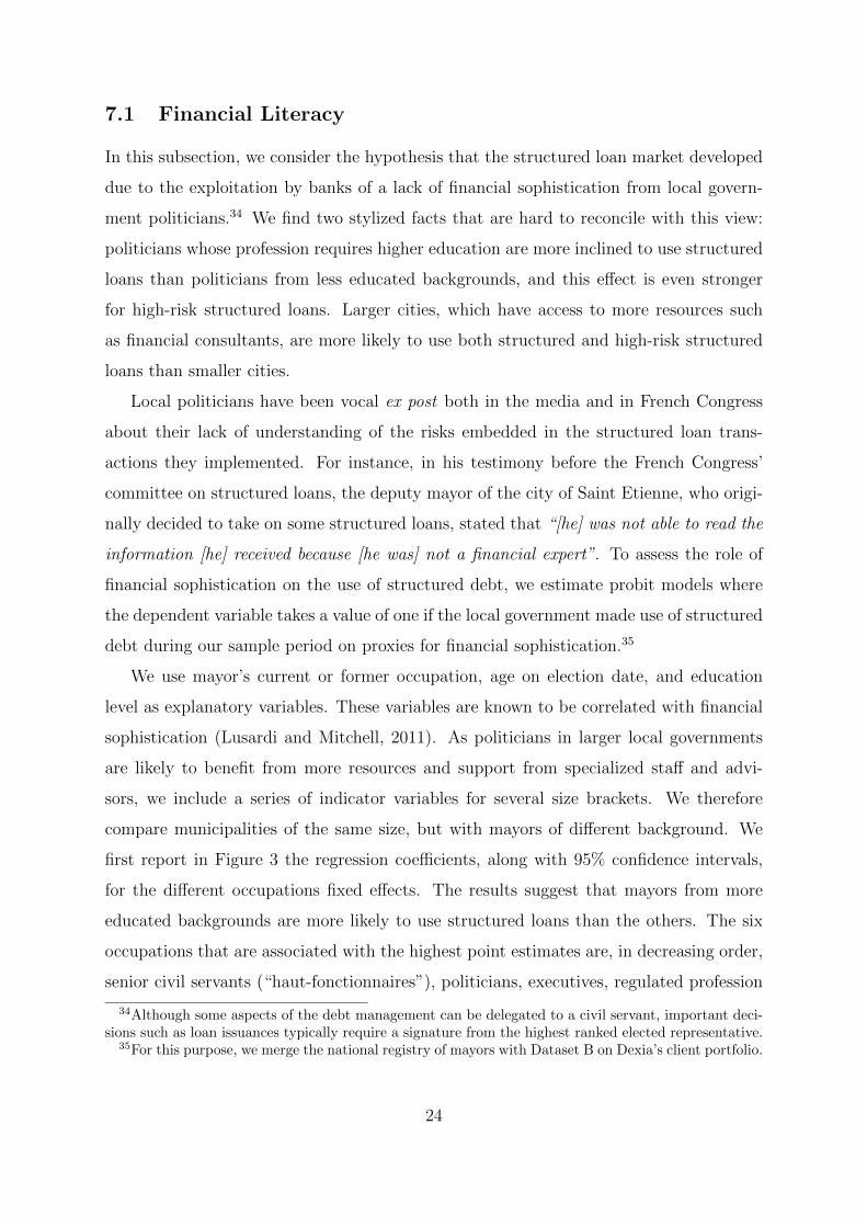
first report in Figure 3 the regression coefficients, along with 95% confidence intervals,

for the different occupations fixed effects. The results suggest that mayors from more

educated backgrounds are more likely to use structured loans than the others. The six

occupations that are associated with the highest point estimates are, in decreasing order,

senior civil servants (“haut-fonctionnaires”), politicians, executives, regulated profession

34Although some aspects of the debt management can be delegated to a civil servant, important deci-sions such as loan issuances typically require a signature from the highest ranked elected representative.

35For this purpose, we merge the national registry of mayors with Dataset B on Dexia’s client portfolio.

24

(doctors, lawyers), engineers, and A-level civil servants.36

[Insert Figure 3 here]

Table 7 provides the coefficients of probit regressions where the dependent variable is

an indicator variable for the use of structured loans in columns 1, 3, and 5, and for the

use of high-risk structured loans in columns 2, 4, and 6. We observe that the likelihood

to use structured loans significantly increases with local government size, and decreases

with mayor age.37 We conduct a more precise test in columns 5 and 6: when restricting

the sample to mayors who are public servants, for whom we can precisely infer their

education level, we find that more educated mayors are more likely to have implemented

structured transactions. Overall, these results are hard to reconcile with the hypothesis

that the development of this market is due to banks exploiting politicians’ lack of financial

sophistication.

[Insert Table 7 here]

7.2 Hedging

Structured loans may have been used as hedging devices. However, there are two main

reasons to rule out this alternative hypothesis. First, the payoffs of structured products

are typically nonlinear and convex because of the embedded sale of out-of-the-money op-

tions. Therefore, to hedge through these instruments, a local government needs to have

operational cash flows that present a strong surplus during tail events for the structured

loan underlying indices, such as EURUSD or the slope of the interest rate curve, which

seems unlikely. Second, French local government revenues appear to be uncorrelated

with the financial indices on which structured loans rely. We indeed calculate the corre-

lation between French local government revenues and the main indices that are used in

structured products: Euribor 3 months, Swap Rate 10Y - Swap Rate 2Y, EURCHF, and

EURUSD. Our analysis covers all French regions, counties, and the 100 largest cities, for

the 1999-2010 period. Overall, we find little to no correlation between revenues and finan-

cial indices (results are available in Table A5 in the Appendix D). We also run a pooled

36A-level civil servants are defined as roles for which a college degree is required to apply, B-levelcivil servants are defined as roles for which a high school diploma is required to apply, and C-level civilservants are defined as role for which no degree is required.

37The average mayor’s age is 54 years old.

25

regression of the change in operating revenues for all local governments on the change in

the financial indices used to structure the loans while controlling for inflation. The esti-

mated parameters that are associated with the financial indices also remain insignificant.

This finding is consistent with empirical evidence of corporations using so-called hedging

policies to make directional bets (Baker et al., 2005).

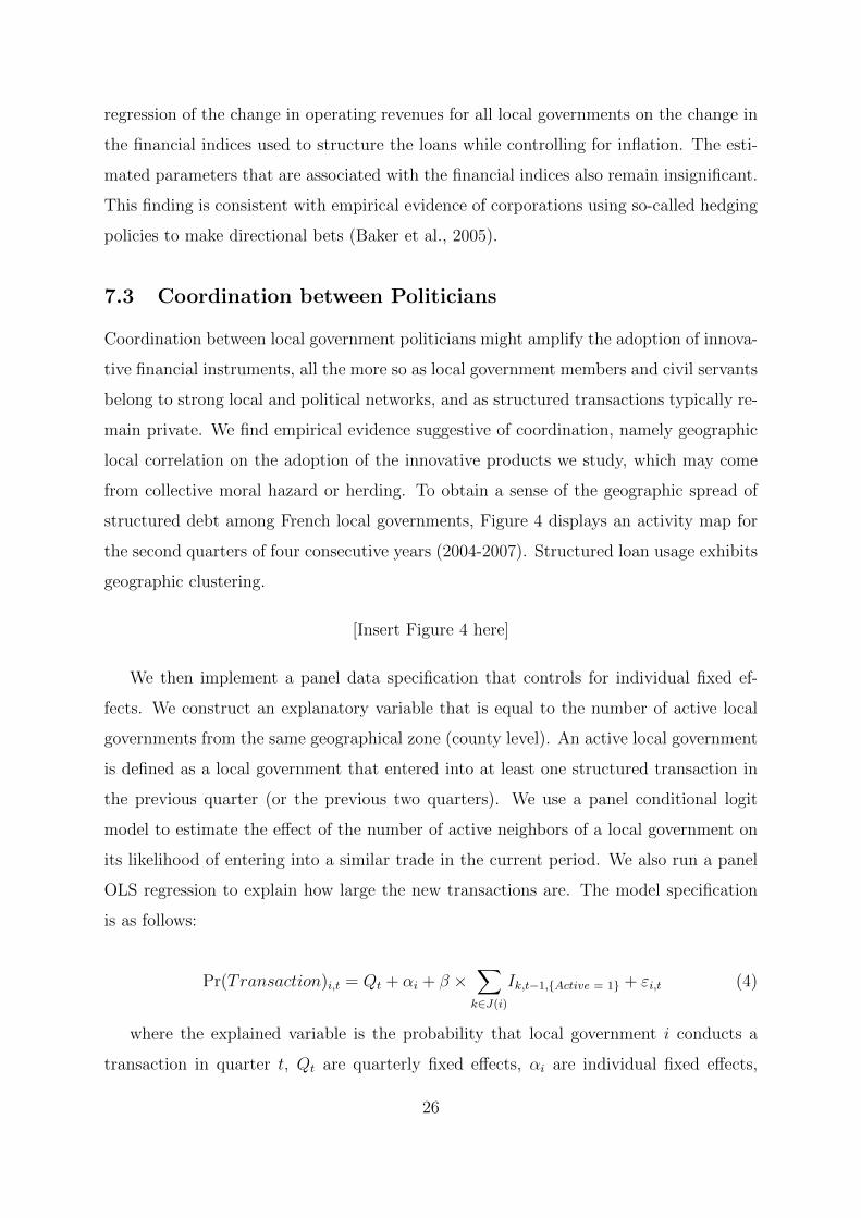
7.3 Coordination between Politicians

Coordination between local government politicians might amplify the adoption of innova-

tive financial instruments, all the more so as local government members and civil servants

belong to strong local and political networks, and as structured transactions typically re-

main private. We find empirical evidence suggestive of coordination, namely geographic

local correlation on the adoption of the innovative products we study, which may come

from collective moral hazard or herding. To obtain a sense of the geographic spread of

structured debt among French local governments, Figure 4 displays an activity map for

the second quarters of four consecutive years (2004-2007). Structured loan usage exhibits

geographic clustering.

[Insert Figure 4 here]

We then implement a panel data specification that controls for individual fixed ef-

fects. We construct an explanatory variable that is equal to the number of active local

governments from the same geographical zone (county level). An active local government

is defined as a local government that entered into at least one structured transaction in

the previous quarter (or the previous two quarters). We use a panel conditional logit

model to estimate the effect of the number of active neighbors of a local government on

its likelihood of entering into a similar trade in the current period. We also run a panel

OLS regression to explain how large the new transactions are. The model specification

is as follows:

Pr(Transaction)i,t = Qt + αi + β ×∑k∈J(i)

Ik,t−1,{Active = 1} + εi,t (4)

where the explained variable is the probability that local government i conducts a

transaction in quarter t, Qt are quarterly fixed effects, αi are individual fixed effects,

26

J(i) is the set of local governments from the same county as local government i, and

Ik,t−1,{Active = 1} is an indicator variable that is equal to one if local government k was

active in quarter t − 1. In the OLS specification, the left-hand-side variable is replaced

by the aggregated notional amount of transactions implemented by local government

i in quarter t. Table 8 displays the conditional logit and OLS regression coefficients.

The coefficients on the number of active local governments is positive and statistically

significant in all specifications. The likelihood and the extent to which a local government

enters into structured debt transactions appears therefore to increase with the number of

active neighbors in the previous period. This result cannot be caused by a time trend, as

we use quarter fixed effects. This effect shows relatively low persistence, as the estimated

coefficients decrease when we consider two quarters.

[Insert Table 8 here]

Politicians might coordinate to decrease their reputation costs in case the transactions

go wrong (Scharfstein and Stein, 1990), or to increase the likelihood of a bailout by

the central government, which would represent a form of collective moral hazard, as

rationalized in Farhi and Tirole (2012).38 Alternatively, the local correlation can also

stem from a purely behavioral herding, where politicians are intrigued or reassured by

other politicians following the same strategy.39

8 Conclusion

In this paper, we present evidence consistent with financial innovation acting as an ampli-

fier of principal-agent problems in the political system. We find that most local politicians

implemented structured loan transactions, as these types of loans account for a surpris-

ingly high 20% of their total outstanding debt. We find that such loans are utilized

38As the bailout would be implemented by the central state, this is a departure from the principal-agent framework we developed. Principal and agent indeed have aligned incentives to obtain a bailout.Although this bailout did happen, it is important to note that it was only partial. The central stateseemed therefore wary not to create moral hazard.

39A final explanation for this correlation in borrowing choices would be the existence of local supplyshocks. However, as Dexia covered the entire French territory before the inception of the structureddebt market, this finding cannot be driven by new branch openings. The arrival of a highly convincingsalesperson in a given region might also create such local shock, although this appears unlikely to driveour results over the whole French territory.

27

significantly more frequently within local governments that are highly indebted, which

is consistent with their greater incentives to shift interest payments to the future. In-

cumbent politicians from politically contested areas are also more likely to use structured

debts, and transactions are more frequent before elections than after elections. We finally

show that using structured loans helps politicians get re-elected, and that they allowed

politicians to maintain lower local tax for their voters.

During the subprime crisis, securitization facilitated a political agenda of easy access

to home ownership. Similarly, we show that financial institutions designed financial

securities fitting politicians’ agenda.

Our results convey potential regulatory implications. Rather than banning structured

loans, we suggest imposing strict public disclosure requirements on transactions by lo-

cal governments to increase reputation risk and facilitate monitoring by voters, which

has been proven to be efficient (Ferraz and Finan, 2008). Furthermore, changing public

accounting standards to account for mark-to-market losses and gains should curb the

incentives by increasing transparency, as observed in comparable markets (Jenter et al.,

2011). Such changes would limit the use of structured loans while maintaining the au-

tonomy of local governments in terms of financial decisions. However, the greatest risk

of structured loans likely lies in outstanding transactions and the accompanying non-

realized losses. The recent bailout of structured loan users answers only partially to this

challenge.

28

References

Amromin, G., J. Huang, C. Sialm, and E. Zhong (2013). Complex Mortgages. Working Paper .

Aneja, A., M. Moszoro, and P. T. Spiller (2015). Political Bonds: Political Hazards and theChoice of Municipal Financing Instruments. NBER Working Paper .

Ang, A., R. Green, and Y. Xing (2014). Advance Refundings of Municipal Bonds. WorkingPaper .

Baker, M., R. S. Ruback, and J. Wurgler (2005). Behavioral Corporate Finance: A Survey. InHandbook in Corporate Finance: Empirical Corporate Finance (Elsevier ed.).

Barrot, J.-N. and J. Sauvagnat (2015). Input Specificity and the Propagation of IdiosyncraticShocks in Production Networks. Working Paper .

Becker, B. and V. Ivashina (2014). Reaching for Yield in the Bond Market. Journal of Finance,Forthcoming .

Behn, M., R. Haselmann, T. Kick, and V. Vig (2014). The Political Economy of Bank Bailouts.Working Paper .

Bertrand, M., F. Kramarz, A. Schoar, and D. Thesmar (2007). Politicians, Firms and thePolitical Business Cycle: Evidence from France. Working Paper .

Besley, T. (2006). Principled Agents? The Political Economy of Good Government. OxfordUniversity Press.

Besley, T. and A. Case (1995). Does Electoral Accountability Affect Economic Policy Choices?Evidence from Gubernatorial Term Limits. Quarterly Journal of Economics, 769–798.

Bharath, S., S. Dahiya, A. Saunders, and A. Srinivasan (2011). Lending Relationships and LoanContract Terms. Review of Financial Studies 24 (4), 1141–1203.

Butler, A., L. Fauver, and S. Mortal (2009). Corruption, Political Connections, and MunicipalFinance. Review of Financial Studies 22 (7), 2873–2905.

Celerier, C. and B. Vallee (2015). Catering to Investors through Complexity. Working Paper .

Centre des Donnees Socio Politiques (2015). Municipal Election Results: 1981 to 2008.

Degryse, H. and S. Ongena (2005). Distance, Lending Relationships, and Competition. Journalof Finance LX, 231–266.

Dessaint, O. and A. Matray (2015). Do Managers Overreact to Salient Risks? Evidence fromHurricane Strikes. Working Paper .

Dinc, S. (2005). Politicians and Banks: Political Influences on Government-Owned Banks inEmerging Markets. Journal of Financial Economics 77 (2), 453–479.

Farhi, E. and J. Tirole (2012). Collective Moral Hazard, Maturity Mismatch, and SystemicBailouts. American Economic Review 102 (1), 60–93.

Faulkender, M. and M. Petersen (2006). Does the Source of Capital Affect Capital Structure?Review of Financial Studies 19 (1), 45–79.

29

Ferraz, C. and F. Finan (2008). Exposing Corrupt Politicians: The Effects of Brazil’s PubliclyReleased Audits on Electoral Outcomes. Quarterly Journal of Economics 123 (2), 703–745.

Gennaioli, N., A. Shleifer, and R. Vishny (2012). Neglected Risks, Financial Innovation, andFinancial Fragility. Journal of Financial Economics 104 (3), 452–468.

Halling, M., P. Pichler, and A. Stomper (2014). The Politics of Related Lending. Journal ofFinancial and Quantitative Analysis, Forthcoming .

Imberman, S., A. Kugler, and B. Sacerdote (2012). Katrina’s Children: Evidence on the Struc-ture of Peer Effects from Hurricane Evacuees. American Economic Review 102 (5), 2048–2082.

Jensen, M. C. and W. H. Meckling (1976). Theory of the Firm: Managerial Behavior, AgencyCosts and Ownership Structure. Journal of Financial Economics 3 (4), 305–360.

Jenter, D., K. Lewellen, and J. Warner (2011). Security Issue Timing: What Do ManagersKnow, And When Do They Know It? Journal of Finance LXVI (2), 413–443.

Julio, B. and Y. Yook (2012). Political Uncertainty and Corporate Investment Cycles. Journalof Finance LXVII (1), 45–83.

Lusardi, A. and O. S. Mitchell (2011). Financial Literacy around the World: An Overview.Journal of Pension Economics and Finance 10 (4), 497–508.

Morse, A. (2011). Payday Lenders: Heroes or Villains? Journal of Financial Economics 102 (1),28–44.

Novy-Marx, R. and J. Rauh (2011). Public Pension Promises: How Big Are They and WhatAre They Worth? Journal of Finance LXVI (4), 1211–1249.

Rajan, R. G. (2006). Has Finance Made the World Riskier? European Financial Manage-ment 12 (4), 499–533.

Rajan, R. G. (2010). Fault lines: How hidden fractures still threaten the world economy. Prince-ton Press.

Scharfstein, D. and J. Stein (1990). Herd Behavior and Investment. American EconomicReview (June), 465–479.

Shiller, R. J. (2013). Finance and the good society. Princeton Press.

Simsek, A. (2013). Speculation and Risk Sharing with New Financial Assets. Quarterly Journalof Economics 128 (3), 1365–1396.

Stock, J. H. and M. Yogo (2005). Testing for weak instruments in linear IV regression. Iden-tification and Inference for Econometric Models: Essays in Honor of Thomas Rothenberg ,80–108.

Wooldridge, J. M. (2002). Econometric analysis of cross section and panel data. MIT Press.

Zingales, L. (2015). Does Finance Benefit Society? Journal of Finance, Forthcoming .

30

9 Figures0

100

200

300

400

500

600

700

800

Num

ber

of S

truc

ture

d Lo

ans

2000 2002 2004 2006 2008 2010Year

Total Of which High-Risk

Figure 1: Number of Structured Debt Transactions per Semester

Note: This figure displays the number of structured loans initiated during a given semester by local gov-ernments in France for the 2000-2009 period. The data are obtained from Dexia’s client portfolio (DatasetB). High-risk structured loans include structured loans indexed to the slope of the interest curve and toforeign exchange rates.

31

Figure 2: Structured Loan Usage and Indebtedness

1030

5070

90%

Use

r

1 2 3 4

Structured Loan Usage

1030

5070

% U

ser

1 2 3 4

High-Risk Structured Loan Usage

1020

30%

Tot

al D

ebt

1 2 3 4

Share of Structured Loans

05

10%

Tot

al D

ebt

1 2 3 4

Share of High-Risk Structured Loans

Note: This figure displays summary statistics on the frequency and the extent of structured and high-riskstructured loan usage for Dataset A. The local governments are ranked into quartiles of indebtedness, calcu-lated as total debt / population. Quartile 1 represents the local governments with the lowest indebtedness,and quartile 4 the ones with the highest.

32

Senior Civil Servant

Professional Politician

Executive

Engineer

Regulated Professions

Civil Servant (Cat. A)

Farmer

Worker

Civil Servant (Cat. C)

Craftman

Civil Servant (Cat. B)

Artist

Journalist

-.1 0 .1 .2 .3

Figure 3: Occupation Fixed Effect

Note: This figure displays the estimated coefficients on mayor occupation title fixed effects from a probit regression ofusing structured loans on local government characteristics and elected mayor demographic variables. The data are fromdataset B merged with data provided by the French Ministry of the Interior. The sample is restricted to municipalities.Dots represent the coefficient estimates, and lines the 95% confidence interval, using standard errors clustered at the countylevel.

33

43

F igure 1: G eographical Evolution of Structured Debt Activity

Year 2004 Year 2005

Year 2006 Year 2007

Notes: This figure displays the number of active local governments, which are defined as those that have

implemented at least one structured debt transaction in the second quarter of the displayed years (from 2004 to

2007). Q2 is the period in which the recently voted budget is financed. Map division is at the department level.

The data are obtained from Dexia!" client portfolio (Dataset B).

Figure 4: Geographical Evolution of Structured Debt Activity

Note: This figure displays the number of active local governments, which are defined as those that have implemented atleast one structured debt transaction in the second quarter of the displayed years (from 2004 to 2007). Q2 is the periodin which the recently voted budget is financed. Map division is at the French county level. The data are obtained fromDexia’s client portfolio (Dataset B).

34

10 Tables

Table 1: Debt Profile of Local Governments

Amount % Total Debt

(in Million Euros) N Aggregate % Use Mean Max Mean Max

Dataset A: Local Government Debt Portfolios

Total Debt 293 51,994.7 95.6% 177.5 1,850.5 - -

Standard Loans and Bonds 293 34,611.5 94.9% 118.1 1,265.6 66.6% 100%

Revolving Facilities 293 6,953.2 58.4% 23.7 646.2 13.4% 100%

Structured Loans 293 10,429.9 72.4% 35.6 648.3 20.1% 95.5%

High-Risk Str. Loans 293 4,372.0 43.0% 14.9 509.9 8.4% 71.7%

Dataset B: Loan Level Data on Structured Loans

Total Debt 1,579 33,423.1 100.0% 21.2 1,870.50 - -

Structured Loans 2,742 23,680.0 100.0% 8.6 459.3 49.7% -

High-Risk Str. Loans 2,742 13,462.0 42.7% 4.9 459.3 28.3% -

Negative MtM 2,742 3,884.1 99.1% 1.4 147.4 8.1% -

# Structured Loans 2,742 - - 1.9 20 - -

Note: This table contains summary statistics on debt profile for two samples of French local governments.All debt figures are expressed in millions of euros. Dataset A is obtained from a survey conducted by aspecialized consulting firm as of December 31, 2007, and includes 25 regions, 96 counties, 76 intercities, and96 municipalities. Dataset B is obtained from Dexia and covers the entire client portfolio of this bank as ofDecember 31, 2009. The sample aggregated total debt represents 38% of all-local-government aggregatedtotal debt. High-Risk Str. Loans are high-risk structured loans, as defined in Section 2. Negative MtMrepresents the unwinding costs for converting structured loans into market-rate vanilla loans.

35

Table 2: Indebtedness and Structured Loan Usage

Dataset A Dataset B

Usage Magnitude Usage(Probit) (Tobit) (Probit)

Structured High-Risk Structured High-Risk Structured High-Risk

(1) (2) (3) (4) (5) (6)

Debt/Population 2.081*** 0.679*** 0.182*** 0.090*** 0.334*** 0.243***4.29 7.53 6.22 10.52 4.07 4.23

Equipment Expenditure/Pop. -0.004*** -0.001* -0.000** -0.000** 0.000*** 0.000-3.71 -1.67 -2.07 -2.44 3.57 0.61

Wages/Operating Expenditure 3.809*** 0.965 0.128* 0.043 0.066 0.9285.51 0.94 1.76 0.26 0.11 0.89

Log (Population) 0.070*** 0.085*** 0.013*** 0.012*** 1.510*** 1.547***3.56 8.13 4.79 6.06 29.09 20.39

Debt Average Maturity 0.075*** 0.057*** 0.015*** 0.015*** - -2.99 3.05 3.31 4.50

Lender FE Yes Yes Yes Yes - -Local Government Type FE Yes Yes Yes Yes Yes YesCounty FE - - - - Yes YesPseudo R2 / R2 0.304 0.181 0.522 0.475 0.436 0.445Observations 275 275 263 263 25,023 22,701

Note: This table contains the probit and tobit regression coefficients using debt portfolio data from a sampleof local governments (Dataset A) for columns 1 to 4, and data from Dexia’s client portfolio (Dataset B)for columns 5 and 6. The dependent variable is an indicator variable for the use of structured products forcolumns 1 and 5, and an indicator variable for the use of high-risk structured loans (as defined in section2) for columns 2 and 6. For columns 3 and 4, the dependent variable is equal to the ratio of structureddebt over total debt, and high-risk structured debt over total debt. Local governments with no debt areexcluded from the regressions of columns 3 and 4. We estimate tobit regressions with left-censoring at zero,and right-censoring at one. Standard errors of the coefficients are clustered by types of local government,and z/t-statistics are reported below the coefficients. *, **, and *** represent statistical significance at the10%, 5%, and 1% confidence levels, respectively.

36

Table 3: Indebtedness and Structured Loan Usage: IV Analysis

Dataset B

Debt/Population Probit

First Stage Structured High-Risk

(1) (2) (3)

Affected (Floods) 0.134**2.21

Debt/Population 1.791*** 2.151**2.90 2.22

Equipment Expenditure/Pop. 0.002 -0.003*** -0.003**1.52 -2.30 -1.78

Wages/Operating Expenditure -0.668* 3.042*** 3.254***-1.96 5.81 3.61

Population Category FE Yes Yes YesCounty FE Yes Yes YesPseudo R2 / R2 0.026 0.357 0.350Observations 32,699 33,739 31,151

Note: This table contains coefficients for an instrumental variable analysis. Column 1 presents the OLScoefficients of the first stage, using floods as an instrument for indebtedness. The floods indicator variableis equal to 1 if the municipality suffered from floods between 2002 and 2008. Columns 2 and 3 display thecoefficients of the second stage of the IV analysis, where the dependent variable is a indicator variable forhaving implemented structured loans during the 2002-2008 period in column 2, and an indicator variablefor having implemented high-risk structured loans during the 2002-2008 period in column 3. Indebtednessis instrumented as per the first stage. Sample is restricted to municipalities. Standard errors of thecoefficients are clustered at the county level, and z/t-statistics are reported below the coefficients. *, **,and *** represent statistical significance at the 10%, 5%, and 1% confidence levels, respectively.

37

Table 4: Politically Contested Areas

Dataset B

Structured Loan Usage

(1) (2) (3) (4)

Stronghold -0.336**-2.07

Years in Power -0.124**-2.06

# Swings 0.185*1.77

Close 2001 Election 0.524*1.82

Margin of Victory in 2001 0.3050.82

Equipment Spending / Population 0.002 0.002 0.002 0.0021.28 1.28 1.37 1.39

Wage / Operation Expenditure 0.151 0.102 0.331 0.1980.12 0.08 0.26 0.15

Log(Population) 0.408*** 0.409*** 0.405*** 0.412***3.22 3.19 3.22 3.20

Pseudo R2 0.018 0.006 0.007 0.009Observations 571 571 571 571

Note: This table contains probit regression coefficients using data from Dexia’s client portfolio (DatasetB). The dependent variable is an indicator variable for the use of structured products. Stronghold is anindicator variable equal to one when the local governments have been ruled by the same party for more than12 years. Y earsinpower refers to the number of years during which the political party of the incumbent(as of year 2001) has been managing the local government. #Swings is the number of changes in politicalcolor during the period 1983-2001. Close 2001 Election is an indicator variable equal to one if the marginof victory was below 5% in the 2001 election. Sample is restricted to municipalities with more than 9,000inhabitants, for which elections results are available. Standard errors of the coefficients are clustered bytypes of local government, and z/t-statistics are reported below the coefficients. *, **, and *** representstatistical significance at the 10%, 5%, and 1% confidence levels, respectively.

38

Table 5: Difference-in-Differences Estimation of Election Timing Effects

Panel A

C-logit Structured Trade Placebo C-logit+\- 18 months + \- 12 months + \- 18 months + \- 12 months

(1) (2) (3) (4)

Pre-Election*Treatment 0.3522*** 0.3350*** 0.0262 0.02752.88 3.28 0.10 0.07

Local Governments FE Yes Yes Yes YesQuarter FE Yes Yes Yes YesRegression Type Panel Panel Panel PanelR2 / Pseudo R2 0.082 0.055 0.053 0.081Periods 12 8 12 8Local Governments 2,741 2,741 2,741 2,741Observations 32,892 21,928 32,892 21,928

Panel B

OLS Structured Trade Placebo OLS+\- 18 months + \- 12 months + \- 18 months + \- 12 months

(1) (2) (3) (4)

Pre-Election*Treatment 0.0218* 0.0280** 0.0010 0.00012.03 2.77 0.00 0.01

Local Governments FE Yes Yes Yes YesQuarter FE Yes Yes Yes YesRegression Type Panel Panel Panel PanelR2 / Pseudo R2 0.0961 0.1240 0.096 0.124Periods 12 8 12 8Local Governments 2,741 2,741 2,741 2,741Observations 32,892 21,928 32,892 21,928

Note: Panel A of this table contains the conditional logit (C-logit) regression coefficients that are estimatedusing data from Dexia’s client portfolio (Dataset B). The dependent variable is an indicator variable ofa structured trade for a given local government in a given quarter. In columns 1 and 2, the explanatoryvariable is an interaction variable between an indicator variable for the treatment group (local governmentshaving an election at the end of 2008Q1) and an indicator variable for the pre-election period. Columns3 and 4 present a placebo analysis in which the treatment group indicator variable that is used in theinteraction term has been replaced by an indicator variable on a random sample of similar size. PanelB replicates Panel A using OLS regressions. Standard errors are clustered by type of public entity. Z/t-statistics are reported below the coefficients. The time window is 18 months before and after the election(end of March 2008) for columns 1 and 3, and 12 months for columns 2 and 4. Standard errors areclustered at the local government level. *, **, and *** represent statistical significance at the 10%, 5%,and 1% confidence levels, respectively.

39

Table 6: Political Effects of Structured Loan Usage: IV Analysis

Probit/OLS First Stage IV

Re-election ∆ Local Tax Structured Loan re-election ∆ Local Tax(Probit) per Inhabitant Usage (Probit) per Inhabitant

(1) (2) (3) (4) (5)

Distance to Dexia Branch -0.002**-2.18

Structured Loan Usage 0.015 11.760** 1.634*** -48.221*0.68 2.45 2.97 -1.72

Debt per Inhabitant 0.002 0.284 0.141*** -0.007 0.7991.36 0.72 4.23 -1.03 1.59

Dexia Branch FE Yes Yes Yes Yes YesPolitical Party FE Yes Yes Yes Yes YesMayor Profession FE Yes Yes Yes Yes YesPopulation Bracket FE Yes Yes Yes Yes YesPseudo R2 0.146 0.027 0.363 0.108 0.026Observations 24,948 25,527 25,190 24,420 25,725

Note: This table contains the coefficients for OLS and an instrumental variable analysis, using distanceto the closest Dexia branch as an instrument for structured loan usage. Columns 1 and 2 display theProbit/OLS coefficients. Column 3 presents probit coefficients for the first stage, where the dependentvariable is an indicator variable equal to one if the local government has borrowed with a structured loanbetween 2002 and 2007. Columns 4 and 5 display the coefficients of the second stage, where the dependentvariable is an indicator variable equal to one if voters elect in 2008 a politician from the same party asthe one elected in 2002 in column 4, and the variation in local tax per inhabitant between year end 2002and year end 2007 in column 5. The variable structured loan usage is instrumented as per the first stage.Z/t-statistics are reported below the coefficients. Standard errors are clustered at the Dexia branch level.*, **, and *** represent statistical significance at the 10%, 5%, and 1% confidence levels, respectively.

40

Table 7: Financial Sophistication

Probit

Structured High-Risk Structured High-Risk Structured High-Risk(1) (2) (3) (4) (5) (6)

1,000 < Pop ≤ 5,000 0.558*** 0.142*10.365 1.792

5,000 < Pop ≤ 10,000 1.721*** 1.300***30.216 14.575

10,000 < Pop ≤ 50,000 2.104*** 1.774***22.978 16.012

50,000 < Pop ≤ 100,000 2.537*** 2.494***10.203 10.892

100,000 < Pop ≤ 200,000 2.256*** 2.226***6.211 5.990

200,000 < Pop 3.027*** 2.880***4.578 5.159

Age at Election -0.004* -0.008**-1.890 -2.166

Senior Civil Servant 0.945*** 4.586***2.577 10.024

College Degree 0.455** 4.442***1.973 15.690

County FE Yes Yes Yes Yes Yes YesPopulation Control No No Yes Yes Yes YesCluster County County County County County CountyPseudo R2 0.280 0.275 0.333 0.327 0.458 0.439Observations 35,712 31,084 26,068 20,027 765 768

Note: This table presents coefficients from probit regressions, where the dependent variable is an indicatorvariable equal to one if the local government has borrowed with at least one structured loan in columns1, 3 and 5, and with at least one high-risk structured loan in columns 2, 4 and 6, during the period 2002-2007. Explanatory variables X < Pop ≤ Y represents indicator variables on whether the local governmentpopulation is between X and Y. Sample is restricted to municipalities. Age at election represents the mayor’sage when elected in the 2001 elections. Columns 5 and 6 further restrict the sample to municipalitieswhose mayor is a civil servant. Senior Civil Servant is an indicator variable for the mayor being a “HautFonctionnaire”, a highly selective status associated with graduating from Elite schools. College Degree isan indicator variable for the mayor having a civil servant status requiring a college degree. Standard errorsare clustered at the county level. *, **, and *** represent statistical significance at the 10%, 5%, and 1%confidence levels, respectively.

41

Table 8: Local Correlation in the Borrowing Choices of Politicians

C-logit Structured Trade OLS ∆(Structured Debt Notional)

(1) (2) (3) (4)

# of Active Neighbors 0.0183*** 10.3991***(Previous Quarter) 5.53 3.03

# of Active Neighbors 0.0064** 4.3144*(Previous Semester) 1.91 1.81

Quarter FE Yes Yes Yes YesRegression Type Panel Panel Panel PanelR2 / Pseudo R2 0.155 0.149 0.010 0.010Periods 40 39 40 39Local Governments 2,741 2,741 2,741 2,741Observations 109,640 106,899 109,640 106,899

Note: This table contains the conditional logit (C-logit) and OLS panel data regression coefficients thatare estimated using data from Dexia’s client portfolio (Dataset B). The dependent variable is an indicatorvariable of a structured trade for a given local government in a given quarter (or semester) for the conditionallogit regressions and the incremental exposure on structured debt entered into by a local government ina given quarter (or semester) for the OLS regressions. The explanatory variable is the number of activelocal governments in the same geographical zone (county level), which is defined as the number of publicentities that have implemented at least one structured transaction in the previous quarter (or semester).The regressions include individual local government fixed effects. Standard errors are clustered by typeof local government. Z/t-statistics are reported below the coefficients. *, **, and *** represent statisticalsignificance at the 10%, 5%, and 1% confidence levels, respectively.

42

- For Online Publication -

Appendix A - Types of French Local Government

Regions (Regions): Metropolitan France is divided into 22 administrative regions,which are in turn divided in 2 to 8 counties (Departements). Regions were created in1982, and do not possess separate legislative authority. One of their primary responsibil-ity is to build high schools, and regional transport infrastructures. In 2004, the medianpopulation of a region in metropolitan France was 2.3 million inhabitants. Regions arefunded partly by the central government, partly by local taxes. Regions are governed bya directly elected council, the Conseil Regional, which in turn elects the council president.

Counties (Departements): Metropolitian France is divided into 96 counties. Theywere created in 1791 following the French Revolution, and do not possess separate leg-islative authority. One of their primary responsibility is to build junior high schools, andcounty-level transport infrastructures. In 2004, the median population of a county inmetropolitan France was 520,000 inhabitants. Counties are funded partly by the centralgovernment, partly by local taxes. Counties are governed by a directly elected council,the Conseil General, which in turn elects the council president.

Municipalities (Communes): Metropolitian France is divided into 36,681 municipal-ities. Municipalities were created in 1789, at the beginning of the French Revolution.Municipalities build primary schools, touristic equipments, and local transport infras-tructure. Municipalities population varies widely, from 10 inhabitants to 2.2 million inParis. Municipalities are funded partly by the central government, partly by local taxes.Municipalities are governed by a directly elected council, the Conseil Municipal, whichin turn elects the mayor.

Intercities (Communautes d’Aglomeration): Intercities are associations of munici-palities. Intercities typically cover a commuting zone. Their primary motive is to financeinfrastructures that cover several municipalities, for instance swimming pools and pub-lic transport. Intercities are mainly funded by its members, which are municipalities.Intercities are governed by a council that comprises the mayors and counsellors of theparticipating municipalities. The council in turn elects the intercity president.

Social Housing Entities (Organismes HLM): Social housing entities own and man-age more than 4 millions housing units, or 17% of primary residences in France. Theboard members are appointed by local governments (counties or municipalities) and theFrench central government. The board nominates a CEO, who has a significant autonomy.

Hospitals (Centres Hospitaliers): Hospitals in France are state-owned, have a gen-eral interest mission, and are non-profit. Hospitals are funded by health insurance organ-isms, local governments, and the central government. Their CEOs are appointed by theHealth Ministry.

43

Appendix B - Structured Loan Types

Products are presented by increasing level of risk according to the Gissler classification.For each type of products, summary statistics are provided in Table A1.

Barriers on Domestic Rate (Gissler Scale: 1)These products lower cost of funding as long as the underlying index is above/under apredefined barrier. Subsidy comes from the premium of the options sold, which could beinterest rate caps or floors. An example is the implicit sale of a floor:

Rate(t) =

{US Libor(t)− x bps if US Libor(t) > 3%

3% otherwise.

Coupon structure does not include any leverage effect. Both the subsidy offered to clientand the bank margin are low (≤ 0.50% of notional). Barriers were the first products toenter the market in the late 1990s. Their interest rate formula can be broken down intoits standard loan component and an embedded short put option:

Standard loan interestrate : US Libor(t)

Sale of a putwith a 3% strike :

{− x bps if US Libor(t) > 3%

3% − US Libor(t) otherwise.

Inflation Products (Gissler Scale: 2)This type of products is usually based on a barrier or on an inflation spread. They ofteninclude leverage to provide with sufficient subsidy, as inflation volatility is very low. Astandard payoff is:

Rate(t) = Midswap(t) − 50 bps + 2 × Max(French Inflation(t) − Euro Inflation(t), 0%).

This illustrates the client’s view that the French inflation rate should remain below theEuropean inflation rate, which could be caused by entrance of new EU members fromEastern Europe with higher inflation.

Steepeners (Gissler Scale: 3)In a Steepener structure, the interest rate is indexed to the Constant Maturity Swap(hereafter CMS) curve slope and decreases the cost of funding when the slope of thecurve is steep; but increases the cost when the curve is flat or inverted. The CMS curveis built with the equivalent fixed rates obtained when swapping Libor for all possiblematurities. They are based on different measures of the slope: [20-year swap rate - two-year swap rate], [30-year swap rate - one-year swap rate], and in most cases [10-year swaprate - two-year swap rate]. An example of payoff is:

Rate(t) = 7%− 5× (CMS 10Y (t)− CMS 2Y (t)).

Entering into a Steepener transaction represents a bet against the realization of forwardlevels, which typically anticipate a flattening of the swap curve. The risk profile of these

44

products is higher than the one of Barrier products. This is mainly due to the introduc-tion of leverage in the interest rate formula, usually without any cap.

Quantos (Gissler Scale: 4)They represent variable interest rate products that are indexed to a foreign interest ratewith an affine formula. They exploit low spot rates and higher forward levels. Risk ismoderate as leverage is generally low and the underlying foreign interest rate has lowvolatility. They are mainly structured on indices from countries with low interest rates,such as Japan or Switzerland. A standard Quanto payoff is:

Rate(t) = 2× JPY Libor(t) or Rate(t) = 1.5× CHF Libor(t) + 1%.

FX Products (Gissler Scale: Out of Scale)FX products are also based on an implicit sale of options. However FX option premiumsare much higher due to the high volatility of foreign exchange rates and remain higheven when strike levels are far from spot prices. This comes from the absence of mean-reversion of foreign exchange rates in banks’ pricing models. This feature allows tostructure products with seemingly unreachable strikes, especially when historical levelsbias the client’s view. An example of payoff for an FX product is:

Rate(t) = 3% + 50%×Max(1.44− EURCHF (t), 0%).

These products offer very high interest rate subsidy, especially on long maturity loanswhen they bear no caps. One example is the 0% interest rate loan by Depfa with Villede Saint Etienne on a 32-year maturity loan. The interest rate is set at 0% for 9 yearsand remains at this level afterwards as long as EURCHF is above EURUSD.

Cumulative Structures (Gissler Scale: Out of Scale)Cumulative structures can be structured on any underlying index: domestic/foreign in-terest rates, FX rates, or inflation rates. They are based on an iterating interest rateformula. Rate degradations therefore add up to each other. The formula often includesa click feature that makes all degradations permanent; hence their nickname: snow balls.Cumulative instrument structuring is based on selling a portfolio of forward-start options.A typical interest rate profile is:

Rate(t) = Rate(t− 1) + 2×Max(USD Libor 12M(t)− 6%, 0%).

Due to the iterating definition of the interest rate, frequency of interest rate payment iskey for the risk profile of the product. For a given leverage level, a quarterly cumulativestructure is four times more aggressive than an annual one. These products have beendramatically impacted by the increase in volatility during the financial crisis, as theybear no cap. They are usually more sensitive to volatility than to market direction (i.e.,vega dominates delta).

45

Appendix C - Figures

Figure A1: Map of Dexia Branches

46

Appendix D - Tables

47

Table A1: Structured-Debt Breakdown

Notional Notional / Local Gov. Total Debt

All Regions Counties Intercities Cities All Regions Counties Intercities Cities

Aggregate 10429.9 1128.5 4801.9 1334.7 3164.91. BarriersAggregate 4970.7 532.3 1959.8 746.8 1731.8Share in % 47.70% 47.20% 40.80% 56.00% 54.70%Mean 17 21.3 20.4 9.8 18 10.20% 6.50% 8.80% 9.90% 12.70%Stdev 33.3 29.2 33.3 24 39.7 14.10% 8.70% 11.90% 17.20% 14.60%Max 342 99.2 161.7 167.9 342 95.50% 33.30% 67.90% 95.50% 69.90%% of use 57.70% 56.00% 60.40% 44.70% 65.60%2. SteepenersAggregate 2794.8 301.1 1417.5 329.4 746.7Share in % 26.80% 26.70% 29.50% 24.70% 23.60%Mean 9.5 12 14.8 4.3 7.8 5.20% 3.50% 5.80% 4.90% 5.30%Stdev 25.4 33.8 33.5 10.1 21 9.70% 11.20% 8.80% 9.30% 10.50%Max 275.8 162.4 275.8 54.4 151.4 70.50% 54.10% 41.60% 44.70% 70.50%% of use 39.90% 32.00% 51.00% 31.50% 37.50%3. FXAggregate 1543.9 87.2 968.3 152.5 335.8Share in % 14.80% 7.70% 20.20% 11.40% 10.60%Mean 5.3 3.5 10.1 2 3.5 2.10% 1.10% 2.50% 2.50% 1.80%Stdev 24.1 11.4 38.4 7.2 14.2 7.40% 3.80% 7.70% 9.40% 6.20%Max 240.8 52.9 240.8 47.4 112.6 66.70% 17.60% 44.00% 66.70% 36.80%% of use 14.00% 12.00% 18.80% 13.20% 10.40%4. InflationAggregate 357.8 102.3 120.2 30.7 104.5Share in % 3.40% 9.10% 2.50% 2.30% 3.30%Mean 1.2 4.1 1.3 0.4 1.1 0.60% 1.40% 0.40% 0.30% 0.70%Stdev 6.6 12.4 7 2.1 6.4 3.50% 5.50% 1.70% 1.50% 4.90%Max 64.4 49 64.4 12.9 60 46.10% 27.00% 11.90% 8.70% 46.10%% of use 7.20% 16.00% 8.30% 3.90% 6.30%5. QuantosAggregate 249.4 33.5 89.4 28.6 98Share in % 2.40% 3.00% 1.90% 2.10% 3.10%Mean 0.9 1.3 0.9 0.4 1 0.50% 0.40% 0.40% 0.30% 0.80%Stdev 3.5 4.2 3.4 2.4 4 1.90% 1.20% 1.30% 1.20% 2.70%Max 33.2 15.8 25.6 20.7 33.2 16.40% 1.20% 8.10% 7.80% 16.40%% of use 12.30% 12.00% 12.50% 6.60% 16.70%6. CumulativeAggregate 33.4 13 7.4 0 13Share in % 0.30% 1.20% 0.20% 0.00% 0.40%Mean 0.1 0.5 0.1 0 0.1 0.00% 0.10% 0.00% 0.00% 0.00%Stdev 1 2.6 0.8 0 0.8 0.30% 0.40% 0.30% 0.00% 0.30%Max 13 13 7.4 0 7.1 3.20% 2.00% 3.20% 0.00% 1.90%% of use 1.70% 4.00% 1.00% 0.00% 3.10%7. OthersAggregate 300.9 30 143.6 28.9 98.5Share in % 2.90% 2.70% 3.00% 2.20% 3.10%Mean 1 1.2 1.5 0.4 1 0.80% 0.30% 1.00% 0.50% 1.00%Stdev 4 4.4 4.6 2 4.5 3.70% 1.00% 3.70% 2.90% 4.50%Max 35.8 20 23.6 12.9 35.8 36.10% 3.40% 27.90% 22.10% 36.10%% of use 8.50% 8.00% 11.50% 3.90% 9.40%

Note: This table contains summary statistics on the different types of structured debt for a sample of Frenchlocal governments, as of December 31, 2007 (Dataset A). The left panel of this table displays statistics onaggregated and local government-level amounts of debt. Figures are in millions of euros, except for sharein % and % of use. Aggregate denotes the sum of the debt notional amount over all local governments.Share in % represents aggregated amount of a given debt instrument in the sample divided by aggregatedtotal structured debt of the sample. The right panel displays statistics on the relative breakdown by debtinstruments at the local government level. For instance, a local government whose debt consists in EUR70mof standard bank loans and EUR30m of FX linked debt will be considered as a local government with 30%of FX linked debt.

48

Table A2: Indebtedness and Type of Borrowing Instrument

Dataset A

Probit

RevolvingLoans

Bonds FloatingRateLoans

(1) (2) (3)

Debt / Population 0.000 0.000 0.0020.00 0.68 0.97

Equipment Spending / Population -0.001 0.002*** -0.002-1.50 2.80 -0.84

Wages / Operation Expenditure 2.118 6.421*** 8.421***1.18 7.07 18.30

Debt Average Maturity 0.027** 0.021 0.198***2.20 0.60 7.33

Log(Population) -0.006 0.663 -0.166-0.80 1.12 -1.16

Lender FE Yes Yes YesLocal Government Type FE Yes Yes YesPseudo R2 0.185 0.526 0.682Observations 275 275 229

Note: This table contains coefficents of probit regressions. The dependent variable is an indicator variablefor the use of revolving loans in column 1, and an indicator variable for the use of bonds in column 2, andan indicator variable for the use of floating rate loans in column 3. Sample data are as of December 31,2007. Standard errors of the coefficients are clustered by types of local government, and z/t-statistics arereported below the coefficients. *, **, and *** represent statistical significance at the 10%, 5%, and 1%confidence levels, respectively.

49

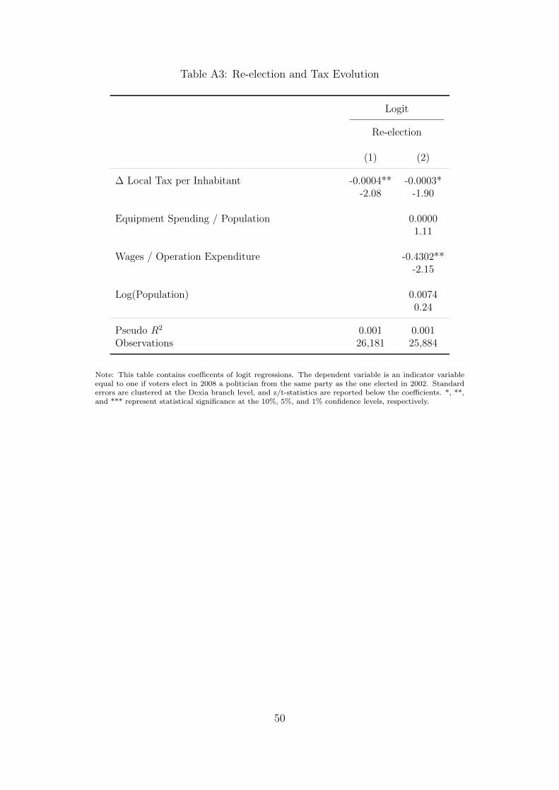
Table A3: Re-election and Tax Evolution

Logit

Re-election

(1) (2)

∆ Local Tax per Inhabitant -0.0004** -0.0003*-2.08 -1.90

Equipment Spending / Population 0.00001.11

Wages / Operation Expenditure -0.4302**-2.15

Log(Population) 0.00740.24

Pseudo R2 0.001 0.001Observations 26,181 25,884

Note: This table contains coefficents of logit regressions. The dependent variable is an indicator variableequal to one if voters elect in 2008 a politician from the same party as the one elected in 2002. Standarderrors are clustered at the Dexia branch level, and z/t-statistics are reported below the coefficients. *, **,and *** represent statistical significance at the 10%, 5%, and 1% confidence levels, respectively.

50

Table A4: Effects of Structured Loan Usage: Breakdown

High-Risk Non-High-Risk

OLS IV OLS IV

Re-election ∆ Local Tax Re-election ∆ Local Tax Re-election ∆ Local Tax Re-election ∆ Local Taxper Inhab. (Probit) per Inhab. per Inhab. (Probit) per Inhab.

(1) (2) (3) (4) (5) (6) (7) (8)

Structured Loan Usage -0.053 -3.835 0.040** 16.232***-1.386 -0.439 2.461 3.308

Structured Loan Usage (IV) 2.209*** -136.300** 2.312**** -40.2992.673 -2.216 2.999 -0.76

Debt per Inhabitant 0.002 0.410 0 1.207* 0.002 0.343 0.010 0.5291.597 0.970 0.027 1.746 1.388 0.869 0.954 1.320

Dexia Branch FE Yes Yes Yes Yes Yes Yes Yes YesPolitical Party FE Yes Yes Yes Yes Yes Yes Yes YesMayor Profession FE Yes Yes Yes Yes Yes Yes Yes YesPopulation Bracket FE Yes Yes Yes Yes Yes Yes Yes YesPseudo R2 0.146 0.026 0.109 0.206 0.146 0.027 0.108 0.026Observations 24,948 25,527 21,962 22,791 24,948 25,527 24,025 24,878

Note: This table contains the coefficients for OLS and an instrumental variable analysis, using distance to theclosest Dexia branch as an instrument for structured loan usage. The specification replicates Table 6, usingas the main explanatory variable an indicator variable for high-risk structured loan usage in columns 1 to 4,and an indicator variable for using non-high-risk structured loans only. Standard errors are clustered at theDexia branch level. *, **, and *** represent statistical significance at the 10%, 5%, and 1% confidence levels,respectively.

51

Table A5: Hedging

Pooled Regression Individual Regressions

Coefficient St. Err. P-value Mean Coeff. St. Dev.Coeff.

% Coeff >0 at 10%signif.

% Coeff <0 at 10%signif.

Euribor 3m -0.0162 0.0168 0.436 0.0122 0.047 3.98% 0.00%

CMS 10y - CMS 2y -0.0601 0.0504 0.355 -0.0193 0.0404 13.72% 1.33%

EURCHF -0.112 0.0963 0.364 0.237 0.3277 15.49% 3.54%

EURUSD 0.1681 0.1577 0.398 0.0982 0.2713 3.98% 0.00%

Note: This table contains summary statistics on regression coefficients between the annual percentagechange in revenues and the percentage change in several financial indices. The pooled regression is runon the four indices, controlling for inflation and with local authorities type fixed effects. Standard errorsof coefficients are clustered by type of local authorities. Individual regressions are conducted for eachlocal government on each individual index, also controlling for inflation. Euribor 3m is the 3-month Eurointerbank offered rate and CMS stands for Constant Maturity Swap and corresponds to the fixed rateobtained by swapping a Euribor interest rate. For CMS 10y - CMS 2y, we use the first difference. Thesample includes all French regions, departments, as well as the 100 largest cities (226 French local authoritiesin total) for which we have revenue data between 1999 and 2010. Index data are from Datastream andlocal authorities’ revenues are from the French Finance Ministry.

52