NBER WORKING PAPER SERIES

THE POLITICAL RISKS OF FIGHTING MARKET FAILURES:SUBVERSION, POPULISM AND THE GOVERNMENT SPONSORED ENTERPRISES

Edward L. Glaeser

Working Paper 18112http://www.nber.org/papers/w18112

NATIONAL BUREAU OF ECONOMIC RESEARCH1050 Massachusetts Avenue

Cambridge, MA 02138May 2012

I am grateful to Yueran Ma and Kristina Tobio for research assistance. The Taubman Center for Stateand Local Government provided financial support. The views expressed herein are those of the authorand do not necessarily reflect the views of the National Bureau of Economic Research.

NBER working papers are circulated for discussion and comment purposes. They have not been peer-reviewed or been subject to the review by the NBER Board of Directors that accompanies officialNBER publications.

© 2012 by Edward L. Glaeser. All rights reserved. Short sections of text, not to exceed two paragraphs,may be quoted without explicit permission provided that full credit, including © notice, is given tothe source.

The Political Risks of Fighting Market Failures: Subversion, Populism and the GovernmentSponsored EnterprisesEdward L. GlaeserNBER Working Paper No. 18112May 2012JEL No. D0,G0,H0

ABSTRACT

There are many possible ways of reforming the Government-Sponsored Enterprises that insure mortgagesagainst default, including a purely public option, complete privatization or a hybrid model with privatefirms and public catastrophic insurance. If the government is sufficiently capable and benign, eitherpublic intervention can yield desirable outcomes; the key risks of any reform come from the politicalprocess. This paper examines the political risks, related to corruption and populism, of differing approachesto the problems of monopoly, externalities and market breakdowns in asset insurance. If there is ahigh probability that political leadership will be induced to pursue policies that maximize the profitabilityof private entities at the expense of taxpayers, then purely public options create lower social losses.If there is a high probability that leaders will pursue a populist agenda of lowering prices or borrowingcosts, then catastrophic risk insurance can lead to lower social losses than either complete laissez-faireof a pure public option.

Edward L. GlaeserDepartment of Economics315A Littauer CenterHarvard UniversityCambridge, MA 02138and NBEReglaeser@harvard.edu

3

I. Introduction

The Federal Housing Finance Agency projects that the bailouts of the Federal Home

Loan Mortgage Corporation (Freddie Mac) and the Federal National Mortgage

Association (Fannie Mae) will require between 220 and 311 billion dollars (“FHFA

Updates”). It is striking that two enterprises, allegedly operating without any government

guarantee, received a bailout bigger than the gross domestic product (GDP) of Ireland or

Egypt, but the financial distress and ensuing bailout were hardly unexpected. For many

years before the downturn, analysts warned of ensuing disaster, while the market treated

their securities as if they were essentially backed with the full faith and credit of the

United States government (Jaffee 2006).

In response the crisis, observers have offered the full range of reform proposals

ranging from complete public control of Fannie and Freddie to total government exit

from the mortgage-insurance business. These proposals have swirled within a larger

debate over banking sector regulation and taxation, where advocates have urged bank

size limitations, bans on proprietary trading, and Tobin taxes, and even temporary

nationalization. In some cases, it is difficult to understand what even the most well-

managed public intervention would achieve, but in every case, it is difficult to assess the

political risks that may distort any reform operation.

Freddie Mac and Fannie Mae might be privatized with stern assurances that even

though the government has bailed them out in the past, this will never, ever happen again,

but should investors believe those assurances? The institutional rules may be written to

prevent bailouts, but those rules can be changed; profit-making mortgage insurance giants

will certainly have the resources and incentives to influence congress and regulators. The

institutional arrangements for Fannie Mae and Freddie Mac will face the twin political

risks of subversion, where private companies capture policy (Stigler 1971), and political

favoritism, where public leaders use government policy to pursue their own pet

objectives, such as populism.

4

These risks help determine the consequences of any institutional reform. If private

mortgage insurer entities are replaced with a purely public mortgage entity, then political

leaders may seek to use that entity for political benefits that are barely related to general

welfare. If the private entities are re-privatized, then their new leaders may be able to

influence the system and again obtain de facto free public insurance for a private entity.

Such political risks are endemic in any public response to market failure, and the

benefits of reducing market failures can be offset by the risks of political failure. Public

ownership once seemed like a reasonable response to the downsides of natural

monopolies, which is why distinguished Progressive Era economists, such as Ely (1901)

argued for municipal ownership of utilities and transit systems. Yet public ownership has

often been associated with operating losses, and allegations of excessively generous

union contracts (Pashigian 1976). Since Stigler (1971), economists have argued that

regulatory agencies, such as the Interstate Commerce Commission, are often captured by

the industries that they are meant to control.

This paper examines the impact of the competing political risks of corruption and

political favoritism in three settings with market failures. The paper follows the

institutional design literature (e.g. Laffont and Tirole 1991) and assumes that the broad

contours of the policy are set optimally, but that the implementation of the policy faces

the risks of private influence and public malfeasance. In these settings, the risk of

corruption is modeled by assuming that with some probability policies are implemented

to maximize the profits of a favored firm (or firms). The risk of political favoritism is

addressed by assuming that, with some probability, political leaders just seek to

maximize the well-being of some segment of society. In this paper, I typically refer to

favoritism as populism and assume that populist leaders favor the poor, but a more

realistic assumption might be that politicians favor the strongest political groups, which

might mean public sector unions or agricultural workers or the wealthy.

In the formal models, the risks of corruption and populism are treated as exogenous

variables that help determine optimal institutions. Section II of this paper discusses the

forces that determine these risks. While there is significant evidence suggesting that

cultural norms strongly influence corruption (Fisman and Miguel 2007), there is also

5

ample room for using the tools of economics to make sense of the incidence of corruption

(Becker and Stigler 1974). For example, the scale of profits that can be achieved by

subverting public officials will surely help determine whether public officials are

subverted. Political favoritism will be more likely if politicians are tied to particular

population subgroups (Alesina, Baqir and Easterly 1999) or if subgroups have an

unusually powerful role in determining elections.

Section III then re-examines two problems which provide a clear motivation for

public intervention—monopoly and externalities—in light of the risks of corruption and

populism. I consider four possible approaches to the problem of a natural monopoly:

laissez-faire, price regulation, quantity-subsidies and total public ownership. I assume

away all of the standard reasons why any particular intervention cannot achieve the first

best, so that in the model, a benevolent leader can and will achieve economic efficiency

with any of the interventions. In my framework, the case for and against particular

interventions depends on their strength at resisting the rival risks of corruption (serving

the interests of the monopoly) or populism (serving the interest of those citizens who do

not pay taxes and do not own the corporation).

Laissez-faire creates the standard welfare losses due to underproduction, but there are

no extra risks from either corruption or populism. If the political leader is potentially

corruptible, public ownership will continue to yield the first best outcome, since it does

not produce a private entity able to bribe the public official. In the case of populism,

however, public ownership leads to high social losses from under-pricing (the good will

literally be free in the model), over-consumption and large operating losses.

In the case of a corrupt official, price controls produce the laissez-faire outcome, as

the price ceiling is set at the profit maximizing level, which is the same level chosen by

the monopolist in the absence of the price regulation. Populist produces monopsony level

price controls which produces shortages, but unless the shortages lead to misallocation

across consumers (Glaeser and Luttmer 2003), the social welfare from monopsony may

well be higher than the social welfare from monopoly, depending on whether supply is

more or less elastic than demand.

6

If there is either corruption or populism, the public official will set subsidies at the

highest possible permissible level. This strange congruence, where completely different

motives produce identical policy distortions, reappears regularly in this paper. Maximal

subsidies occur under corruption because subsidies increase the monopolist’s profits.

Populism produces maximal subsidies because the politician’s poorer constituents do not

pay for the taxes needed to pay for the subsidies, yet they benefit from the lower prices

that subsidies produce. The implicit subsidy, through implicit government insurance,

enjoyed by Fannie Mae and Freddie Mac may well reflect a combination of influence by

those companies and a desire by some politicians to favor middle-income borrowers.

When populism is the larger risk, price controls produce more losses, but when

corruption is more common, public ownership leads to higher levels of social welfare.

These results may explain why public ownership seemed natural to many as a solution to

monopoly pricing in late 19th century America. If the political risks of corruption and

populism are sufficiently high, then laissez-faire may produce higher levels of public

welfare than interventions.

When externalities are the problem, instead of monopoly, I consider quantity controls

instead of price controls. Otherwise, the results are similar to the monopoly setting.

Public ownership continues to yield optimal social welfare with corruption and low

pricing with populism. A quantity control leads to the monopoly outcome with

corruption, and either laissez-faire or a monopsony-related quantity limitations with

populism.

If the externality is negative and calls for a Pigouvian tax, then the downside from

corruption or populism is relatively limited if the taxes are used to reduce the other taxes

paid by wealthier taxpayers. Corruption will lead to no regulation, and populism will

lead to a tax between zero and the optimal Pigouvian tax. If the tax does benefit the

politicians’ supporters, then Pigouvian taxes create the danger of significant over-taxing

for revenue purposes. In some circumstances, the risks of populist over-taxing can mean

that there are lower losses from revenue-less taxes (where the tax is pure social loss) than

from revenue raising taxes. This result provides conditions when public campaigns that

7

vilify smoking or drinking sugary soda, which are sometimes linked with libertarian

paternalism may be desirable (Sunstein and Thaler 2009).

If the externality was positive, which calls for a Pigouvian subsidy, then both

corruption and populism again lead to maximal subsidies. As in the monopoly case,

these subsidies can lead to significant welfare losses. As such, political risks create an

important difference between positive and negative externalities and suggest that there is

considerably more risk from subsidies than from taxes, because taxes have a natural

barrier at zero.

In Section IV, I turn to default insurance and regulation in a model that loosely

follows Diamond and Dybvig (1983). Investors lend to borrowers and receive claims on

future income, but they investors may turn out to be impatient and seek to resell those

securities. Private information about the quality of those securities creates the possibility

for a lemons market breakdown that leads to higher borrowing costs ex ante. Default

insurance creates a means of mitigating that problem, but private and public default

insurance creates its own problem. Private insurance companies have an incentive to

issue too little equity, in order to maximize the returns on equity for shareholders during

good states of the world. Limited liability limits the losses during bad states. In some

cases, the public may end up covering the losses of the private insurer to avoid a market

breakdown.

The significant risk in this scenario is the private mortgage insurers have an incentive

to leave themselves under-capitalized. Protected by limited liability, insurers would like

to have negative profits in bad states and higher profits, per unit of investment, in the

good state. By under-capitalizing, the firm increases profitability in the good state and

creates no added costs to shareholders in the high default state, since insurer profits are

zero in the adverse state of nature with high default levels. This creates the risk of under-

funded insurers, which can lead to a breakdown of the entire market.

Again, the public sector can react to this problem with capital requirements, asset

fees, catastrophic risk insurance or outright nationalization. As in the case of banking,

corruption and populism push in the same direction—more subsidized risk-taking.

8

Nationalization tends to be more efficient in the case of corruption, but it creates the

greatest losses from populism. The case for private for public ownership depends on the

relative risks of populism and corruption.

In Section V, I apply this model briefly to the case studies of Freddie Mac and Fannie

Mae. Populism seems to have motivated some political support for these entities, but

they were also aggressive in lobbying and funding political campaigns. Their political

support seems to have generally limited attempts to strongly regulate their activities. By

contrast, public entities, like the Federal Housing Administration (FHA) and Ginnie Mae,

have performed somewhat better which may suggest that populism is less risk than

corruption.

While the model is quite stylized, it does provide some insight relating to the current

debates over Freddie Mac and Fannie Mae. Public intervention of any sort in these

markets is fraught with political risk. The possibility of populism or subversion both

push to excessive risk-taking and insufficient capital reserves. Private ownership creates

none of the protection it provides in more standard scenarios, since the public sector is

still able to spend without limit. If the risk of corruption is sufficiently high, public

ownership may be safer for taxpayers than privatization.

II. Political Risks, Dictatorship and Disorder

The new institutional economics (Djankov, Glaeser, LaPorta, Lopez-de-Silanes and

Shleifer 2003) presents institutional design as a tradeoff between different private and

public welfare losses. In most societies, there is no means of achieving perfection, just

the chance to trade off between public abuses, sometimes referred to as dictatorship, and

private abuses, sometimes referred to as disorder. Countries face an institutional

possibilities frontier offering choices between systems with more dictatorship

(communism) and more disorder (laissez-faire capitalism). The shape of that frontier

depends on cultural and economic fundamentals, such as the level of human capital. One

explanation for Wagner’s Law, the fact that government spending increases more than

proportionally with national income, is that as countries develop the institutional

9

possibilities frontier shifts and citizens increase their ability to control the government

more effectively. As citizens become better at disciplining the state, public interventions

becomes more attractive.

In this paper, I will also address welfare losses coming from two different sources,

and one of those sources is tied to private initiative (corruption) while the other reflects

purely public malfeasance (political favoritism or populism). Yet both issues are

basically examples of “dictatorship,” in the sense that social costs occur through the

action of the state. In the examples, I consider there will also be social losses from

laissez-faire policies and those represent “disorder.”

In the model, I treat the probability of facing a corrupt or populist public leader as

fixed and exogenous but these probabilities actually reflect deeper economic and political

variables. This preliminary section briefly discusses the forces that shift those

probabilities.

The Beckerian (1968) approach to corruption suggests that corruption occurs when

the benefits of accepting money or favors in exchange for subverting public policy

outweigh the costs to the individual. Those costs are likely to include both real penalties,

such as going to jail or losing an election, and psychic costs, which may differ from

culture to culture. In a Coasian world where bargaining is easy, a corrupt bargain should

occur whenever the total benefits of the deal to the private entity exceed the costs to the

public leader.

That logic suggests that the magnitude of the benefits that can accrue from corruption

should help determine the level of corruption. As the economic scale of an activity

increases, the gains from corruption should also increase. Glaeser and Shleifer (2003)

argue that the increasing size of industrial concerns during the 19th century meant that

firm’s ability to bribe increased as well, and that led to a subversion on many institutions,

such as the courts, during the Gilded Age. The move from a tort-based system of

addressing railway-related externalities to greater regulation may have been a response to

the fact that the costs to judges of being corrupt were overwhelmed by the increasingly

large economic rents that came from skewing justice.

10

If bargaining across firms is difficult, especially when trying to arrange for large

bribes, then competition will lead to less corruption risk than monopoly. The political

dangers from concentrated economic entities have led observers from Woodrow Wilson

to Simon Johnson (Johnson and Kwak 2011) to call for size limitations on particular

firms, like large banks. One argument for why larger firms may find regulations

attractive is that there are returns-to-scale in rent-seeking that enable those firms to

particularly excel in subverting the regulator and getting the rules changed to suit their

own needs (Peltzman 1976). In the models, I treat the probability of corruption as being

identical in the case of regulating a natural monopoly and regulating a competitive

market with externalities, but it seems likely that the risk is higher in the case of

monopoly.

Finally, the possible rents from corruption depend heavily on the nature of the

intervention itself. In principle, the problem of combating monopoly under-production

can be addressed with either a price ceiling or a subsidy to production. The profits

gained from subverting the price ceiling are capped at the standard monopoly earnings,

but the profits gained from subverting a subsidy are virtually limitless.

While the benefits that come from corruption may be quite obvious, the costs that

prevent corruption are often less clear. Fisman and Miguel (2007) provide striking

evidence that diplomats from cultures that are thought to be less corrupt are also less

likely to rack up parking tickets while at the United Nations. There is no legal penalty for

these tickets, but still the diplomats from less corrupt cultures have fewer tickets. Does

this reflect a complicated set of social enforcement mechanisms, where Swedish

diplomats are informally punished if they abuse their host community, or has Swedish

culture inculcated a taste for honesty?

While culture surely matters, it certainly seems possible for a strong central leader,

like Lee Kwan Yew, to radically reduce corruption through a combination of severe

penalties and lower standards for proof.i The Beckerian approach may omit important

psychological and cultural forces around wrong-doing, but the probability of arrest and

the size of the punishment still help deter crime. In highly corrupt societies, the

11

probability of arrest often appears to be extremely low, partially because everyone is in

on the game.

When political cultures work to limit corruption, typically officials end up enforcing

rules on each other. Fishback, Kantor and Wallis (2006), for example, present evidence

suggesting that the federal bureaucracy created by New Deal programs significantly

reduced American municipal corruption. The process of creating documents for a

different branch of government created a natural outside observer. American history is

replete with examples, such as the famous Lexow Committee of 1894, where corruption

was investigated by politicians representing a different party who were in power within a

different level of government.

One impact of increasingly tough penalties on overt corruption is that corruption will

take more opaque and more legal forms. If it is no longer possible to pay senators with

paper bags full of cash, then campaign donations and the promise of future favors will

have to suffice. Being forced to use more roundabout and inefficient means of

subversion is essentially a tax on corruption which should reduce its incidence, but that

hardly means that subversion is likely to vanish altogether.

Across countries, corruption is correlated with ethnic fragmentation (Mauro 1995),

French legal origin (Djankov, LaPorta, Lopes-de-Silanes and Shleifer 2003) and

education. That latter correlation also holds for U.S. states (Glaeser and Saks 2006).

These facts may say something about the culture created by education and English

common law or they may reflect political institutions in well educated, former English

colonies that discipline corrupt politicians.

The second political risk is that a political leader may subvert policies in order to

achieve some objective other than maximizing social welfare. As maximizing social

welfare is rarely well-defined, outside of economists’ mathematical models, political

favoritism or populism is rarely punished with criminal sanctions. Instead the costs that

can occur are limited to punishment at the voting booth or perhaps psychic costs to the

politician. Moreover, while corruption is perhaps reasonably approximated with the

assumption of discrete choices—take the bribe or don’t—political favoritism is almost

12

surely a matter of degree in almost every case—how much to slant policies towards a

favored group.

Since we understand so little about the costs of political favoritism to individual

politicians, most of the literature discussing its incidence has focused on the benefits of

such favoritism. Ethnic and cultural fragmentation appear to be associated with

favoritism (Alesina, Baqir and Easterly 1993), either because fragmentation reduces the

consensus on the common good or because it leads to politicians who have close ties with

a particular national subgroup (Glaeser and Shleifer 2005). Politicians who are closely

tied to a particular subgroup are likely to support that group both because of innate

preferences and because they perceive their political futures as being tied to the well-

being of that group. Jim Crow politicians, such as Theodore Bilbo, appear to have

advanced racist policies for both reasons.

Political favoritism should also be more common when particular groups have

disproportionate political influence. For example, critical swing voters should attract

favoritism. Well organized political groups, like public sector unions, should elicit

favoritism. Finally, those groups that are specifically favored by political institutions, as

farmers are by the U.S. Senate, should attract targeted support.

Political favoritism may be less costly if the impact on the favoritism on general well-

being is easy to observe and if the political leader is held electorally accountable for the

community’s success. For that reason, executives, such as mayors, are often thought to

be less prone to such favoritism than legislators, such as city council members, who are

not held responsible for the general success of their locale. Indeed, the tendency to

punish political leaders for widespread local problems is sufficiently strong so that

governors are punished for the pure bad luck of low oil prices or a national recession

(Wolfers 2006).

The political risks of corruption and favoritism do vary greatly across time and space,

but they are never actually non-existent. The next section examines their impact on

standard models of monopoly and addressing externalities.

13

III. Management of Monopoly and Externalities

When there are either externalities or a natural monopoly, laissez-faire fails to

produce the socially optimal outcome. Yet public responses generate their own risks

when politicians are not perfectly benevolent. Here I first examine monopoly and then

externalities and in each setting, I consider four institutional options: (1) laissez-faire; (2)

quantity or price controls; (3) taxes and/or subsidies; and (4) pure public ownership and

control. When the costs of public ownership will only be paid by the rich, I also consider

the possibility that taxes on firms will be given as transfers to the poor.

Following the discussion above, I assume that the government constrained by the

basic institutional options. Laissez-faire gives the government no options whatsoever.

Quantity controls means that the government can reduce firm production as much as it

likes, including shutting the firm down altogether, and price controls can act as either a

floor or a ceiling. In either case, the government cannot force firms to produce more than

they would like given the existing price. Taxes and subsidies can only be levied per unit

produced and there will be an upper limit on the subsidy denoted . This upper limit is

necessary because otherwise, corruption and populism would lead to infinite subsidies.

Moreover, if there is supposed to be a tax it cannot be turned into a subsidy and a subsidy

cannot be turned into a tax. There are no constraints on prices or quantities in the case of

public ownership, except that the government must charge the same price to all

consumers.

In all cases discussed here, I assume that a benevolent government could achieve first

best outcomes under any of the activist regimes. I don’t mean to suggest that there aren’t

informational or organization barriers to producing first best outcomes, even if political

leaders are benign. I assume these issues away to focus on the political risks that may

influence optimal policy. As such, the barriers on government behavior will only become

important if the government is less than benign.

I consider two risks that might afflict the government that is administering policies,

with the limits imposed by the institutional regime: corruption and populism. Corruption

14

occurs with probability and implies that the government has been bribed into doing

the will of the business sector. Government policies will then maximize profits.

Populism occurs with probability , and this state means that the government will

choose policies to maximize the well-being only of the poor citizens. The welfare losses

of populisms will be particularly stark because I assume a starkly utilitarian welfare

function. If the welfare function was more egalitarian, then the social costs of this regime

will be somewhat mitigated.

Managing Monopoly

In this first example, I consider the management of a natural monopoly. The

technological basics of the model are standard. There is a single producer, that has

perhaps paid fixed costs to enter, and that pays a cost C(Q) to produce Q units that are

shared among the N consumers.

Each consumer is ex ante identical, but who randomly become wealthy with

probability or poor with probability 1 . If they are wealthy, they earn a higher

income, own the shares of all produces and pay all taxes. If they are poor, they earn a

lower income, own no shares and pay no taxes. The utility functions of both groups are

V(q)+Income-pq, where q is the quantity consumed of the product, p is its price and V(q)

is weakly concave, and that V’(q)=0 for a finite level of q, which is denoted . The

demand curve for every person rich or poor is V’(q)=p, so everyone consumes the same

amount of the product.

While I will discuss issues of egalitarianism at length, I will assume evaluate different

positive outcomes based on individual’s expected utility as of birth or—equivalently—

the equally weighted purely utilitarian welfare function, which reduces to NV(q)-

C(Nq)+Other Income. Holding consumption of the good constant, the price paid for the

good is essentially a transfer. I will ignore the other income, which does not change

across settings, and let , describe the relevant social welfare

function, which will change across different institutions and political outcomes. The

optimal level of “q,” denoted satisfies ′ ′ ) and produces

15

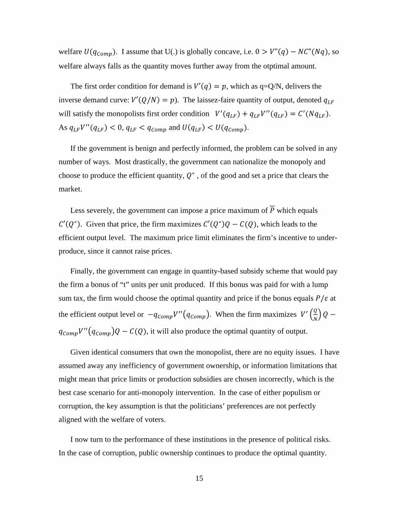
welfare . I assume that U(.) is globally concave, i.e. 0 " " , so

welfare always falls as the quantity moves further away from the otptimal amount.

The first order condition for demand is ′ , which as q=Q/N, delivers the

inverse demand curve: ′ / ). The laissez-faire quantity of output, denoted

will satisfy the monopolists first order condition .

As 0, and .

If the government is benign and perfectly informed, the problem can be solved in any

number of ways. Most drastically, the government can nationalize the monopoly and

choose to produce the efficient quantity, ∗ , of the good and set a price that clears the

market.

Less severely, the government can impose a price maximum of which equals

′ ∗ . Given that price, the firm maximizes ′ ∗ , which leads to the

efficient output level. The maximum price limit eliminates the firm’s incentive to under-

produce, since it cannot raise prices.

Finally, the government can engage in quantity-based subsidy scheme that would pay

the firm a bonus of “t” units per unit produced. If this bonus was paid for with a lump

sum tax, the firm would choose the optimal quantity and price if the bonus equals / at

the efficient output level or . When the firm maximizes

, it will also produce the optimal quantity of output.

Given identical consumers that own the monopolist, there are no equity issues. I have

assumed away any inefficiency of government ownership, or information limitations that

might mean that price limits or production subsidies are chosen incorrectly, which is the

best case scenario for anti-monopoly intervention. In the case of either populism or

corruption, the key assumption is that the politicians’ preferences are not perfectly

aligned with the welfare of voters.

I now turn to the performance of these institutions in the presence of political risks.

In the case of corruption, public ownership continues to produce the optimal quantity.

16

There is no private entity to bribe the politicians and thus even when the politicians are

venal, there is no one to take advantage of their venality. Hence welfare remains

. In reality, a sufficiently corrupt politician will still figure out ways to extract

rents from public ownership, like overpaying for inputs and providing outputs free of

charge in exchange for kickbacks, but these are outside of the scope of the model.

In the case of a price restriction, a corrupt politician serving the monopolies’ interests

cannot do better for the firm than putting the price at the monopoly price. This means

that output will be and welfare will be .

In the case of a subsidy, the problem of corruption automatically leads to the maximal

subsidy, as firm profits are always increasing in the level of the subsidy. The level of

output in the case, denoted satisfies , as the

subsidy regime must admit the optimal subsidy, . The subsidy

must increase the firms’ quantity produced, which will lower welfare beyond the optimal

amount, so higher subsidy limits will always reduce well-being. If is sufficiently high,

the firm may produce beyond the point where the price of the good is zero, and the

welfare from the corrupt regime will be worse than in either alternative institutional

setting or in the case of laissez-faire.

What will populism do under the three different regimes? Since the losses born by

the public company are born by the rich, whom the populism ignores, the populist will set

p=0, which leads to consumption .

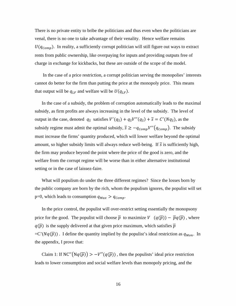
In the price control, the populist will over-restrict setting essentially the monopsony

price for the good. The populist will choose to maximize , where

is the supply delivered at that given price maximum, which satisfies

=C’( . I define the quantity implied by the populist’s ideal restriction as . In

the appendix, I prove that:

Claim 1: If NC N ′′ , then the populists’ ideal price restriction

leads to lower consumption and social welfare levels than monopoly pricing, and the

17

populists’ idea restriction leads to higher consumption and social welfare levels than

monopoly pricing if NC N ′′ .

That claim reminds us that the distortion created by a monopsony price cap can be

larger or smaller than the distortion created by monopoly pricing. The monopsony

distortion is generally smaller when supply is more elastic, i.e. C”(.) is greater, and the

monopoly distortion will be larger when demand is more elastic, i.e. V”(.) is greater.

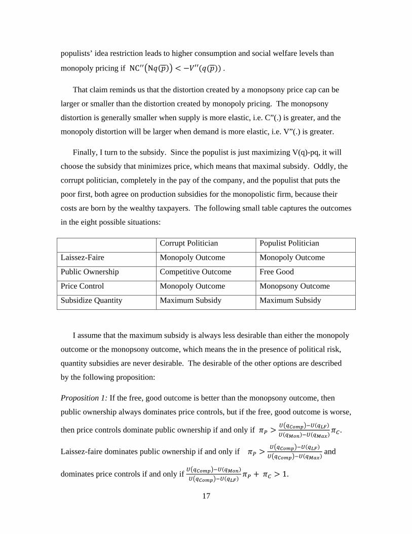
Finally, I turn to the subsidy. Since the populist is just maximizing V(q)-pq, it will

choose the subsidy that minimizes price, which means that maximal subsidy. Oddly, the

corrupt politician, completely in the pay of the company, and the populist that puts the

poor first, both agree on production subsidies for the monopolistic firm, because their

costs are born by the wealthy taxpayers. The following small table captures the outcomes

in the eight possible situations:

Corrupt Politician Populist Politician

Laissez-Faire Monopoly Outcome Monopoly Outcome

Public Ownership Competitive Outcome Free Good

Price Control Monopoly Outcome Monopsony Outcome

Subsidize Quantity Maximum Subsidy Maximum Subsidy

I assume that the maximum subsidy is always less desirable than either the monopoly

outcome or the monopsony outcome, which means the in the presence of political risk,

quantity subsidies are never desirable. The desirable of the other options are described

by the following proposition:

Proposition 1: If the free, good outcome is better than the monopsony outcome, then

public ownership always dominates price controls, but if the free, good outcome is worse,

then price controls dominate public ownership if and only if .

Laissez-faire dominates public ownership if and only if and

dominates price controls if and only if 1.

18

The proposition provides the basic results on how political risks shape the desirable

policies. If high subsidies lead to socially undesirable outcomes, then addressing the

monopoly problem by subsidizing output leads to bad outcomes in the case of either

populism or corruption.

The tradeoff between public ownership and price controls depends on the relative

probability of corruption or populism. In settings where corruption is normal, but

populism is rare, then this makes public ownership more attractive, for public

ownership’s great strength is that it is it does not produce a private entity ready to bribe

the politician. This result may explain why public ownership was relatively popular

during the Progressive Era. In those years, corruption seemed like a great threat and the

perils of populist politicians who could run public utilities at massive losses in order to

placate their constituents may have seemed less apparent.

But political risks also tend to make any intervention less attractive, even when there

is an obvious monopoly problem. If the risks of populism are relatively high, then public

ownership becomes less attractive than laissez-faire. If monopsony is worse than

monopoly and if the risks of both populism and corruption are high, then price controls

may be worse than just allowing the monopolist to function.

Managing Externalities

We now consider a setting where the case for intervention reflects an externality—

good or bad—and making two alternations to the model. First, supply is now made by

measure one of competitive firms, each with cost functions C(Q). In the absence of

subsidies or quantity controls, this leads to first order condition P=C’(Q) which

determines supply. This keeps the core functions identical to the monopoly case, but

drops the assumption that the firm sets prices. I do however assume that if the politicians

are corrupt they will try to maximize the earnings of the entire industry not just a single

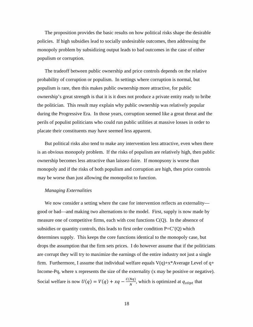
firm. Furthermore, I assume that individual welfare equals V(q)+x*Average Level of q+

Income-Pq, where x represents the size of the externality (x may be positive or negative).

Social welfare is now , which is optimized at that

19

satisfies ′ ′ , which will be greater than if and only if the

externality is positive, i.e. x>0.

The pure laissez-faire case actually yields which would be the first best output

in monopoly case discussed above, but is suboptimal here because of the externalities.

The first best can be achieved through public ownership, which just chooses the optimal

level of output, or through a Pigouvian tax or subsidy equal to “x.” A quantity control

fixing output at would also yield the optimal quantity with a negative externality.

Quantity controls do not provide a natural means of handling a positive externality. In

principle, a fixed price level could also achieve the optimal quantity, but it would do so

by creating shortages and the possibility of misallocation across consumers, so I ignore

that option.

We now consider the impact of corruption and populism on these three interventionist

options. In the case of corruption, public ownership continues to produce the first best

outcome; there is again no private entity to corrupt the political leaders. In the case of a

populist politician, who ignores the wealthy taxpayers costs of funding the operation, the

good is produced and sold to maximize , which means p=0 and quantity

is set so that either ′ (if x is negative) or ′ 0 if the externality is

positive. In the case of a negative externality, the good is sold at a price of zero, and

rationed to individuals. In the case of a positive externality, you would like to force

people to consume beyond the point where V’(q)=0, but that is impossible. I denote the

quantity as , which will equal when x>0 and will be less than if x<0.

This seems likely to be an extremely poor outcome from an efficiency perspective.

In the case of quantity controls and negative externalities, corruption will lead to the

monopoly outcome for firms, called in the previous section; since the corrupt

politician essentially internalizes the firms’ desire to collectively restrict production. This

quantity may actually be above if the externality is negative and severe, but will

lie below if the externality is moderate or positive.

In this case of populism, the government will choose “q” to maximize the value of

, which means that if x<0, quantity will satisfy ′

20

′ 0. The populist is interested in lowering the prices paid by consumers, and

that will reduce its willingness to reduce quantities. Since restricted quantity creates a

gap between supply and demand, price is set by the demand curve and p’(q)=V”(q). The

quantity-controlling populist sets q so that " 0 as long as the “q” implied

by this is below the free market quantity. I denote this quantity (the monopsony

quantity in the presence of an externality). If x is sufficiently large so that the optimal

quantity, implied by ′ ′ 0, is greater than the free market

quantity, a populist government with quantity controls will not intervene since it can only

force firms to produce less than they normally would, not to produce more.

Subsidies, used in the case of a positive externality, will be set to the maximum

amount allowable if the politician is corrupt. If the politician is populist, then the subsidy

will be chosen to maximize . This will also lead to maximum

possible subsidy, since prices fall with the subsidy and there is the added benefit of

increasing the positive externality.

Taxes, used in the case of negative externality, will be set to zero if the politician is

corrupt and trying to maximize industry profits. In the case of a negative externality and

tax, the populist politician’s behavior depends on whether the politician’s poorer

constituents are able to benefit from the tax or whether the tax goes to defray the other

tax costs paid by the wealthy. If the tax revenues benefit only the richer voters, the

populist will choose the tax to maximize , which leads to the

same condition as in the case of the quantity control with a negative externality:

" . Just as in that case, the politician chooses a tax to produce either

(the monopsony amount in the presence of an externality) or the free market quantity,

whichever is smaller. This provides another setting where populism and corruption can

lead to exactly the same outcome.

If the politician’s constituents can benefit from the tax revenues, then the populist

maximizes . I assume that they cannot be targeted

towards the poor in particular, but they can be remitted back to everyone in some form,

like spending on public services. The preferred tax satisfies " , which

21

is higher than the optimal tax. I denote the associated quantity as because the

tax is transferring from firms to the populists constituents.

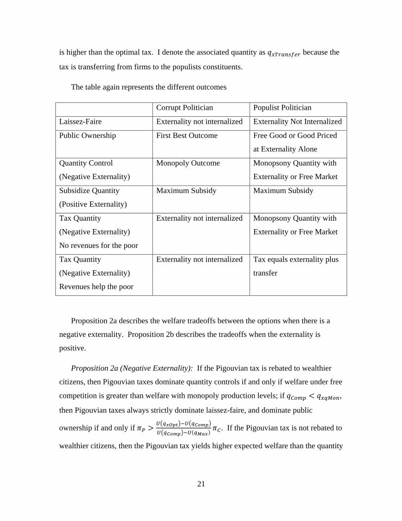
The table again represents the different outcomes

Corrupt Politician Populist Politician

Laissez-Faire Externality not internalized Externality Not Internalized

Public Ownership First Best Outcome Free Good or Good Priced

at Externality Alone

Quantity Control

(Negative Externality)

Monopoly Outcome Monopsony Quantity with

Externality or Free Market

Subsidize Quantity

(Positive Externality)

Maximum Subsidy Maximum Subsidy

Tax Quantity

(Negative Externality)

No revenues for the poor

Externality not internalized Monopsony Quantity with

Externality or Free Market

Tax Quantity

(Negative Externality)

Revenues help the poor

Externality not internalized Tax equals externality plus

transfer

Proposition 2a describes the welfare tradeoffs between the options when there is a

negative externality. Proposition 2b describes the tradeoffs when the externality is

positive.

Proposition 2a (Negative Externality): If the Pigouvian tax is rebated to wealthier

citizens, then Pigouvian taxes dominate quantity controls if and only if welfare under free

competition is greater than welfare with monopoly production levels; if ,

then Pigouvian taxes always strictly dominate laissez-faire, and dominate public

ownership if and only if . If the Pigouvian tax is not rebated to

wealthier citizens, then the Pigouvian tax yields higher expected welfare than the quantity

22

control if and only if

, .

The proposition highlights the relative strength of Pigouvian taxes, especially when

they are not vulnerable to being used for political favoritism. The Pigouvian tax always

dominates laissez-faire, because even if it is subverted, it is likely to only produce the

laissez-faire outcome. As long as free competition is preferable to the monopoly

outcome generated by a corrupt quantity regulator, then the Pigouvian tax is also

preferable to a quantity control, because it is somewhat less vulnerable to abuse. The

comparison with public ownership again depends on the probability of populism vs.

corruption. When corruption is a far greater threat, then public ownership remains the

safer reform. When populism is more common, then the Pigouvian tax yields higher

expected welfare.

When revenues can serve populist purposes, it is not necessarily true that Pigouvian

taxes become worse, but there do appear to be more cases where the Pigouvian tax is

dominated by quantity controls. The revenue-raising tax may not be so bad at all, but it

can be, and the Pigouvian tax can produce less welfare than the quantity control even if

free competition provides better outcomes than the monopoly-like outcome that is created

by a corrupt politician using a quantity control to restrict production.

Proposition 2b (Positive Externality): The Pigouvian subsidy dominates public

ownership if and only if and dominates laissez-faire if and only if

. Public ownership dominates laissez-faire if and only if

.

This proposition suggests that there are many more occasions when laissez-faire is

dominant when externalities are positive than when externalities are negative. Political

risks are relatively contained with Pigouvian taxes, because there is a natural barrier at

zero, but there is rarely such a natural risk with a subsidy. Pigouvian taxes are therefore

relatively safe, even with these political risks, while Pigouvian subsidies are not.

23

Laissez-faire is more attractive than subsidies whenever the combined risk of populism

and corruption are sufficiently high and more attractive than public ownership as long as

the risk of populism is sufficiently great. The tradeoff between public ownership and

subsidies depends on the relative risks of populism, which can make public ownership

riskier, and corruption which increases the risks associated with Pigouvian subsidies.

One implication of this discussion is that limiting the incentives for government

malfeasance may be quite desirable and such limits might be using tax-like instruments

that raise no revenues. One interpretation of psychological approaches to paternalism,

such as advertising depicting the health consequences of smoking to people’s lungs, is

that they are revenue-less taxes that reduce the pleasure of the activity without generating

any associated returns to the treasury. While sometimes these interventions can be

justified as providers of information, there is little evidence supporting the view that

smokers are ignorant of the risks of smoking (Viscusi 1992). The alternative view is that

these interventions create psychological costs when people consume the depicted goods.

George Loewenstein and Glaeser (2009) have both questioned the value of these policies

precisely on these grounds. If politicians were always benevolent, then these taxes would

always be suboptimal relative to using standard Pigouvian taxes.

Yet the presence of political risk, and especially the risk of populist politicians who

like taxing externalities to provide benefits for their constituents, makes such policies

somewhat more attractive. I now consider the possibility that the government can use a

tax, imposed directly on consumers, that generates no revenues. I only treat the case with

negative externalities and I assume, as above, that the tax benefits everyone, not just the

populist politicians’ constituents.

I assume that .5 and .5 .

Proposition 3: If the politicians are benevolent, then the revenue-raising tax is

preferable to the revenue-less tax, and if the politicians are corrupt then no taxes are

raised in either case, but if the politicians are populist, then revenue-less taxes dominate

revenue-raising taxes when x is sufficiently close to zero.

24

The conditions under which a revenue-less tax dominates a revenue-raising tax are

fairly extreme, yet the basic point remains. The revenue-less tax may be subject to less

abuse by a populist politician looking to raise revenues for his favorite constituents. In

extreme cases, this benefit may offset the apparent waste of an intervention that causes

harm to consumers without raising any offsetting revenues.

IV. Bank Runs, Liquidity and Mortgage Insurance

I now turn to the particularly relevant issue of political risks and financial regulation.

I begin with a model of banks and bank runs, borrowing heavily from Diamond and

Dybvig’s classic model of bank runs. I then turn to a model of security-insurance, which

can be interpreted as the mortgage insurance provided by the Government-Sponsored

Enterprises (GSEs). In both cases, laissez-faire creates significant welfare losses, but the

presence of political risks creates potential losses from interventions.

Default Insurance and Political Risk

The following model is an adaptation of Diamond and Dybvig (1983). At time zero,

there are three classes of individuals: investors, non-discretionary borrowers and

discretionary borrowers. Borrowers, of both varieties, are endowed with no units of the

consumption good in periods zero or one, but they may receive one unit of the

consumption good in period two. Non-discretionary borrowers are completely impatient

and only care about consumption at time zero, which is denoted . Discretionary

borrowers maximize , where 1,. It will be socially inefficient for

discretionary borrowers to consume in period zero, rather than period two, and this

creates a potential welfare loss from overly subsidized borrowing. But since these

borrowers will not enter the market unless borrowing is highly subsidized, they will not

figure in the discussion of the model until I turn to government interventions.

Borrowers, of either type have an ex ante probability of receiving no income in

period two. If this occurs, they will default and there is no method of punishing them or

otherwise extracting resources from them. At time one, it is revealed whether default

25

levels among borrowers will be high or low. The unconditional probability of either state

is equal to one-half, and if the default level is high then a proportion ∆ of the

borrowers will default. If the probability of default is low, then a proportional ∆ of

the borrowers will default.

I will primarily consider a lending market where investors give money to borrowers

in period zero and in exchange they receive a claim to the borrowers’ potential income in

period two. These claims are meant to be a stylized version of a mortgage contract

(albeit without collateral) or any other loan, and I will refer to them as debt contracts.

These claims can be traded in period one, but there is a potentially a lemons problem that

can compromise the tradability of the debt contracts. I will later compare this market in

which lending operates through tradable securities with a market served by financial

intermediaries.

At time zero, all investors are endowed with units to invest. I will assume that there

are enough investors, and they have enough income in every period, so that there is never

any shortfall in funds to lend. There are two types of investors—patient and impatient—

and investors learn their type at time one. With probability t, investors are impatient and

receive utility equal to . With probability 1-t, individuals are patient and

have utility equal . As in Diamond and Dybvig (1983), the possibility of

impatient investors creates a benefit from period one liquidity. By assuming that

investors have abundant funds, I ensure that the prices of debt contracts will equal their

expected value to investors in every period. Since discretionary borrowers value the

future more than investors (of either variety), they will not borrow unless borrowing is

subsidized by the state.

In period one, investors learn the aggregate state of the world and whether they are

impatient. They also receive specific information about debt contracts that they have

purchased. Investors who lend to a specific borrower learn whether that individual is low

risk, in which case the probability of default is zero, or high risk, in which case the

probability of default is 1/v. I assume that only one investor will directly learn the

quality of any one asset, which follows a tradition of considering asymmetric information

in the mortgage market (Glaeser and Kallal 1997). It is simpler to assume that there is

26

only one investor for each borrower, which I do, but a lemons problem would also result

even if the asset was shared among investors, as long as only one person knew the

borrower’s quality.

The equilibrium price as of time zero for a claim on one unit of borrower’s

consumption in time two is denoted . Investors are not able to resell these claims until

period one, when they have learned whether or not they are patient and whether or not

their borrower is high risk. Importantly, only the investor knows his own type and the

type of the lender, so that traded securities are effectively anonymous in period one. The

price of a claim for one unit of borrower consumption in period two, as of period one

denominated in period one consumption, is denoted .

The equilibrium price in period one is determined by the willingness-to-pay of

patient investors, and since their utility function is , the price will equal the

expected value of the asset in period two. In period one, there are essentially “types” of

debt contracts that might be sold, categorized by the following box:

Asset Held by patient investors

Held by impatient investors

High Risk

Expected Value=(v-1)/v

Share of Assets Outstanding:

1 ∆ or 1 ∆

Expected Value=(v-1)/v

Share of Assets Outstanding:

∆ or ∆

Low Risk

Expected Value=1

Share of Assets Outstanding:

1 1 ∆ or

1 1 ∆

Expected Value=1

Share of Assets Outstanding:

1 ∆ or 1

∆

Impatient investors who hold high risk securities will always want to sell their

assets, and if they are the only group that sells the price of the asset will be one minus the

default rate or (v-1)/v. However, impatient investors with low risk securities would also

like to front load consumption, and they will always do this if 1 . If that

condition holds, the impatient investors with the safe securities will want to sell, even if

27

they are sure to be perceived as selling high risk securities. It is socially efficient for

those impatient investors to sell, since they value earlier consumption while there is an

abundance of patient investors who do not.

While there is never any welfare gain from patient investors selling their

securities in the first period, patient investors with high risk securities will still want to

sell as long as the sales price is greater than (v-1)/v, as it will be if any low risk, impatient

investors are also selling. Any equilibrium where both groups of impatient investors sell

will also have patient investors dumping risky securities. By contrast, the patient

investors with low risk securities will never sell.

As Proposition 4 describes, there typically are multiple equilibria. The

proposition also describes the time zero price, which will be determined by the expected

benefits to investors of buying the securities in the first place.

Proposition 4: (a) If , then there exists an equilibrium where, in either

state of the world, only impatient investors who have high risk investments sell their

securities and the market price of these securities equals and the price in period zero

equals 1 1 1 .

(b) If ∆

∆, then there also exists an equilibrium where, in either

state of the world, all impatient investors sell their securities in period one and the price

in period zero equals 1 .This equilibrium Pareto dominates the equilibrium with less

trade.

(c) If ∆

∆

∆

∆ , then there also exists an equilibrium

where impatient investors sell all their securities when default rates are low, but only

impatient investors with high risk debts sell when aggregate default rates are high.

The proposition notes that as long as ∆

∆, there is the

possibility for multiple equilibria. In one equilibrium, securities are thought by buyers to

be low quality, prices are low, and only low quality securities are sold. In a second

28

equilibrium, securities are assumed to be mixed in quality, prices are higher and as a

result, impatient investors sell their securities. In the high trade equilibrium, patient

securities with high default risks also sell their securities during the first period. There is

also a mixed equilibrium where a fraction of investors with high quality investors sell

their securities in period one. Since that equilibrium is essentially unstable, I will not

discuss it at length.ii

It is also possible that there is a market breakdown if the aggregate default rate is

expected to be high, since in that case, there are more patient security owners with high

risk securities. Their greater presence in the market reduces the price that impatient

investors with good securities receive in the high trade equilibrium, and lower prices may

cause these groups to leave the market altogether and for a complete lemons market

breakdown to result.

The model can explain why the liquidity of securities is likely to become more of

a problem during periods of greater distress. When the probability of default is low, then

it is easier to sustain the high trade equilibrium, because the number of impatient security

holders with low risk securities is a large share of the selling pool. As the share of sellers

who have high risk securities increases, the quality of pool deteriorates, eventually

causing impatient sellers to just sit on their good securities.

The proposition focuses on equilibria that involve pure strategies, although there

typically also exists (when ∆

∆) an additional equilibrium where

some, but not all, of the impatient investors with low risk securities sell. In that case, the

first period price must equal to make those investors indifferent between selling and

not. That equilibrium is somewhat less interesting because it is inherently unstable. If a

slightly larger fraction of the impatient investors with good securities sell, then the price

of those securities will rise causing all impatient investors to sell. If a slightly lower

fraction of the impatient investors with good securities sell, then the price of those

securities will fall and no investors with good strategies will sell

The potential for a lemons market breakdown creates scope for public

interventions. If the public sector, or the private sector, is able to homogenize the assets,

29

so that all of them carry equivalent risk, then the breakdown can be avoided and

borrower’s welfare will be improved because they will receive higher prices for selling

their claim to second period consumption.

One solution for avoiding the social losses associated with the low trade

equilibrium is for securities to be insured by a public or private entity. The public entity

can be entirely self-financing, although it is also possible to use tax revenues in the

second period. For example, the simplest system would be to charge an up-front fee of

to provide complete insurance against default. This would cover the expected costs of

the system, but the system would earn excess profits in low default states and losses in

high default states. The profits could be returned to taxpayers and the losses could be

funded with taxes on investors (as a group) during the second period. Alternatively, if I

embedded this in a multi-period model, the agency could expect, like the Federal

Housing Administration (a real world analog to public insurance) to earn losses in bad

times and offset them with profits during good times.

The public entity could also totally finance itself with a tax of ∆ . This higher

fee would cover losses in the high default state, and the profits could be returned to the

investors in the form of a 2∆ per security refund if the default rate proves to be low. In

either case, the period zero price of securities equals 1 , their expected value to

patient investors. If politicians are neither corrupt nor populist, then the public insurance

system creates no problems and achieves a liquid market and the first best outcome.

Moreover, since the public insurance company earns no profits, it cannot corrupt

politicians. Just as in the discussion of monopoly and externalities above, if the political

system is corrupt, public insurance will continue to yield the first best outcome.

Populism however creates greater social costs.

I assume that populist politicians are interested in benefitting borrowers, at the

expense of investors. This will lead populists to charge a desultory amount (effectively

zero) for default insurance and finance losses with general tax revenues imposed on

investors. This will represent redistribution from investors to borrowers. Since the

30

security yields a return of one, for sure, in the second period, the period zero price will

also be one.

But this high price also creates an efficiency loss because of the discretionary

borrowers. If the discretionary borrowers sell their claim for period two consumption

during period zero, they will receive one unit of consumption and will receive welfare of

one. But if they don’t borrow, they only receive period two consumption with probability

1 . As long as 1 1 , the populism will lead to inefficient over-borrowing

even by highly patient borrowers. Since they are trading an uncertain claim to future

consumption for the expected value of a sure claim, their borrowing is subsidized.

Public insurance is not the only solution for this lemons breakdown problem. In

principle, private insurance can also homogenize the securities and allow them to be

traded without fear during period one. In this case, borrowers would pay a premium of

for insurance, and the insurance company would also raise equity of at least ∆

∆ per

security insured. The insurance and investment fees would then be lent to borrowers, and

this would provide enough returns to cover investors’ losses in the bad state, and profits

in the good state equal to ∆ ∆

, ortwice the value of the initial investment.

Investors would be willing to buy equities since the expected return is one, and since

there is no asymmetric information about the insurance company risk, its securities could

be readily traded during period one.

The great danger with a private insurance company is that it will issue too little

equity to cover its losses in the high default state of the world. For example, assume that

an insurance company that has raised EQ units of equity to cover an existing portfolio of

Q securities with potential defaults, where E equals ∆

∆ so that the first Q mortgages

were fully insured. The company now decides to insure an extra q mortgages, for which

it will raise eq units of equity.

If “e” is not observable to investors who are insuring their mortgages, then the

incentive to raise too little equity is obvious. If the firm sets e<∆

∆ and is able to

continue charging for insurance, then existing shareholders stockholders will earn

31

nothing in the high default state (which was always true) and EQ ∆ ∗

∆ inthegoodstate, which is strictly decreasing in e. Existing shareholders will

benefit from issuing too little equity to cover losses in the bad state, since they stand to

earn more in the good state.

The insurance company could continue to be able to charge if consumers

incorrectly assess the lack of equity capital by the insurer, or if they believe that the

government will cover the shortfall in the high default state. Indeed, recent events do

suggest that in a high default state, nominally private mortgage insurers, Fannie Mae and

Freddie Mac, will see their obligations paid by the government. This leads security

holders to continue to pay the full fee of , even if the insurance company has insufficient

capital to cover the shortfall.

If the government doesn’t regulate equity and cannot commit not to cover losses

in the adverse state of the world, then competition among insurance companies will

reduce insurance costs to ∆. This is enough to cover losses in the low default state,

and the government will cover extra costs in the bad state. Higher insurance costs would

lead to positive profits that would be competed away. Borrowers will be able to sell their

security for 1 ∆, and in this case, there is an implicit public subsidy that occurs to

lending, and this can lead the discretionary borrowers to borrow excessively.

Discretionary borrowers will also borrow if 1 1 ∆ , or ∆ 1

1 .

Yet even if the government were able to commit to letting the mortgage insurer

fail, there would still be a problem if equity was raised sequentially. If the initial capital

was sufficient to cover shortfalls, then those original shareholders would still have an

incentive to want the firm to issue too little capital to cover losses, even if the investors

buying mortgage insurance correctly anticipate that their mortgages will be insufficiently

covered. This effect continues to reflect the limited liability nature of the company:

Proposition 4: A private insurer with an existing stock of Q insured securities,

that is trying to maximize the expected value of its raised equity, which equals ∆

∆, will

32

want to minimize the equity raised to cover losses from any further insurance contracts,

even if the buyers of those further insurance contracts recognize the risks of insufficient

equity, as long as those risks do not cause a market breakdown in period one.

Any firm with an existing set of insured securities, for which it is has issued

sufficient capital to withstand all losses in good times and bad, has an incentive to raise

too little equity to cover the losses from any further insurance contracts. Even though the

fees paid by the new contracts will be lower, since the insurer recognize the downside of

insufficient equity, the fees paid by the old contracts will not change (they have already

been paid) and those old contracts will also pay the cost of too little equity. The benefit

of having too little equity is that the firms existing equity holders will earn more in the

good state of the world, because their profits in the good state do not get diluted by being

shared with new equity-holders.

In the extreme, after the first share is issued, the company will never want to issue

any more equity and the insurance company becomes equity-free. With equity-less

insurance, individuals will pay a premium of ∆

∆ and as long as the insurance firms

invests in the traded securities, this will provide enough to fully insure defaults during

low default states of the world. During high default states of the world, the insurance

company will be unable to fully cover its obligations, and individuals with borrowers

who default will receive ∆ ∆

∆ ∆1 in the high default state, since that is all the

funding that is available. With equity-less insurance, there can continue to be a period

one market breakdown.

Proposition 5: With equity-less private insurance, if

1 ∆

∆ ∆, then an equilibrium exists where impatient investors and

patient investors with high risk securities sell their partially insured securities in both

states of the world and the initial security price is 1 . With equity-less private

insurance, if 1 ∆

∆ ∆ then an equilibrium exists where impatient investors

and patient investors with high risk securities sell their partially insured securities in the

33

low default state, but only investors with high risk securities sell in the high default state.

In this case, the initial security price is 1 .5 1 1 ∆ 1 ∆ .

The existence of incomplete insurance delivers lower welfare, in the case of the

market breakdown, than complete insurance which avoids such meltdowns. But

incomplete insurance is certainly better than no insurance at all, since without insurance

there can be a market breakdown in good and bad states, but with insurance the

breakdown only occurs in bad states of the world.

I now consider two public interventions when there is private insurance: (1)

public backstop insurance with equity regulation, (2) public backstop insurance with an

insurance fee charged to asset issuers. The government will have the option whether to

extend the insurance scheme to some or all competitors in the industry.

Both schemes can easily produce the first best if the public sector manages them

appropriately. If firms are required to raise equity of at least ∆

∆ per security insured,

then the first best outcome result, and the government will never need to step in. If firms

are charged a catastrophic risk fee of ∆

∆, then this amount will cover losses in the bad

state, and the excess can be refunded to security owners in the good state.

What are the political risks of the two systems? Populist politicians attempt to

ensure that borrowers get the best deal, and that will result in government backstop

insurance without either fees or equity requirements. Just as in the case of no pre-

commitment, competition will ensure that insurance costs ∆, and securities will sell

for one minus that amount. Discretionary borrowers will again borrow if ∆ 1

1 .

In the case of equity requirements, the possibility for corruption occurs because

the state will be able to choose whether or not to grant backstop insurance to any

particular entity. This discretion is assumed to be automatic, as it is hard to imagine that

the state would not have the ability to decide that some firms or not operating with this

support. Despite the government’s difficulties in committing not to bail out Fannie Mae

34

and Freddie Mac, it certainly managed to let large numbers of investors take the hits for

defaults in the subprime market.

A corrupt politician will choose a unique firm to receive the benefit of this

backstop insurance. It will impose neither equity requirements, nor a fee, on that firm.

That firm’s ability to extract profits will still be limited by competition with an uninsured

competitive fringe. In the good state, for each unit of insurance, if the insurance

company charges , the company will earn ∆ ∆, and in equilibrium will

equal 1 , which creates another reason for the company to want to boost insurance

costs. Higher costs mean lower security costs which mean higher profits.

There are two constraints on . The secure public insurance must be more

attractive than unsupported private insurance. If equity-less private insurance leads to no

market breakdown, then will have to be less than or equal to in order to insure that

investors will prefer the publicly backed insurance to equity-less private insurance. In

that case, the public company will earn profits of ∆

in the good state per unit of

insurance. If equity-less insurance leads to a lemons breakdown in the bad state, then the

firm with publicly backed insurance can charge .5 1 1 ∆ 1

∆ and earn commensurately higher profits.

If the insurance price is denoted , then the initial security price will equal

1 , and the extra profits from attracting sales to discretionary borrowers can induce

the publicly backed corrupt company from lowering the insurance cost. Discretionary

borrowers will sell the claim on their second period consumption if 1 1 ,

which requires that 1 1 / . This means that the price must be lower than .

I denote the ratio of non-discretionary borrowers to total borrowers as . The

following proposition illustrates the optimal behavior of the publicly supported company:

Proposition 6: If equity-less private insurance does not lead to a lemons market

breakdown, then the public asset insurance firm charges 1 1 / and sell to

discretionary and non-discretionary borrowers if 1 ∆ 1 ∆ and

will charge and sell only to non-discretionary borrowers otherwise. If equity-less

35

private insurance does lead to a lemons market breakdown, then the public asset

insurance firm charges 1 1 / if 1 ∆ 1 ∆

1 ∆ and otherwise, where q denotes . 5 1 1

∆ 1 ∆ .

This proposition shows that if equity-less private insurance competes with the publicly

supported insurance, the publicly-supported firm will charge a low enough price to attract

the discretionary borrowers if is close to one and if is small. In this case, there

will be welfare losses from excessive borrowing.

If equity-less insurance does lead to a lemons-style breakdown, then the publicly

supported company has more market power with the non-discretionary borrowers and

this makes it less likely that the company will charge a lower price to attract the non-

discretionary borrowers. Even if is arbitrarily close to one, it is possible that the

company will ignore those borrowers and continue to charge a higher fee.

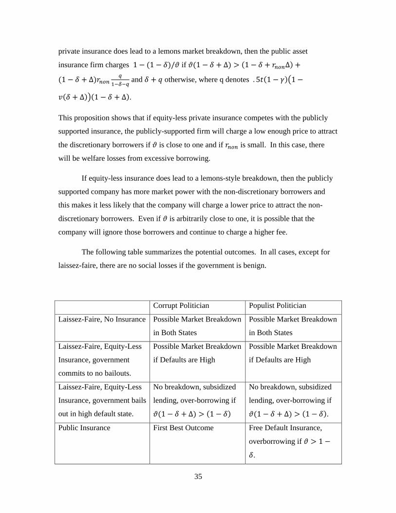
The following table summarizes the potential outcomes. In all cases, except for

laissez-faire, there are no social losses if the government is benign.

Corrupt Politician Populist Politician

Laissez-Faire, No Insurance Possible Market Breakdown

in Both States

Possible Market Breakdown

in Both States

Laissez-Faire, Equity-Less

Insurance, government

commits to no bailouts.

Possible Market Breakdown

if Defaults are High

Possible Market Breakdown

if Defaults are High

Laissez-Faire, Equity-Less

Insurance, government bails

out in high default state.

No breakdown, subsidized

lending, over-borrowing if

1 ∆ 1

No breakdown, subsidized

lending, over-borrowing if

1 ∆ 1 .

Public Insurance First Best Outcome Free Default Insurance,

overborrowing if 1

.

36

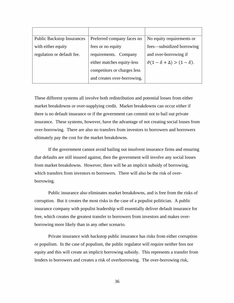
Public Backstop Insurances

with either equity

regulation or default fee.

Preferred company faces no

fees or no equity

requirements. Company

either matches equity-less

competitors or charges less

and creates over-borrowing.

No equity requirements or

fees—subsidized borrowing

and over-borrowing if

1 ∆ 1 .

These different systems all involve both redistribution and potential losses from either

market breakdowns or over-supplying credit. Market breakdowns can occur either if

there is no default insurance or if the government can commit not to bail out private

insurance. These systems, however, have the advantage of not creating social losses from

over-borrowing. There are also no transfers from investors to borrowers and borrowers

ultimately pay the cost for the market breakdowns.

If the government cannot avoid bailing out insolvent insurance firms and ensuring

that defaults are still insured against, then the government will involve any social losses

from market breakdowns. However, there will be an implicit subsidy of borrowing,

which transfers from investors to borrowers. There will also be the risk of over-

borrowing.

Public insurance also eliminates market breakdowns, and is free from the risks of

corruption. But it creates the most risks in the case of a populist politician. A public

insurance company with populist leadership will essentially deliver default insurance for

free, which creates the greatest transfer to borrowers from investors and makes over-

borrowing more likely than in any other scenario.

Private insurance with backstop public insurance has risks from either corruption

or populism. In the case of populism, the public regulator will require neither fees nor

equity and this will create an implicit borrowing subsidy. This represents a transfer from

lenders to borrowers and creates a risk of overborrowing. The over-borrowing risk,

37

however, in this case is less extreme than in the case of a populist public insurance entity

because the size of the subsidy will be smaller.

If the public regulator is corrupt, rather than populist, then this will lead to

monopoly power by a single insurance entity (or perhaps by a cartel of such entities).

This will result either in transfers from investors to the shareholders of this entity and

potentially also to borrowers. Borrowers receive some of the benefits if the firms decides

to cut prices by enough to encourage over-borrowing results.

The decision between the more hard-edged approaches and various public

interventions involves a tradeoff between the risk of market breakdowns and the social

costs of over-borrowing. If the government cannot commit not to bail out private lenders,

then public backstop insurance generally dominates an official system of no backstop

insurance, at least in terms of aggregate welfare, because the government will end up

bailing out the firms anyway. At least if the government functions well, backstop

insurance can produce the first best. If the government suffers from either corruption or

populism, the results will be no worse (again from the perspective of total social welfare)

than in the case of implicit insurance.

The decision between public insurance and backstop insurance with fees or equity

regulation depends on the relative risks of populism and corruption. The public insurance

system is strong if corruption is more likely, but weakest in the case of populist

politicians. Backstop insurance is the better scheme when populism is the greater threat.

The next proposition summarizes the welfare conclusion. To consider social

welfare, I will ignore any transfers across classes of citizens, and assume an additive

social welfare that simply sums up the ex ante expected utility across the three different

groups of investors. This creates two potential sources of social losses: over-borrowing

and illiquidity. If over-borrowing occurs then there is a social loss equal to the number of

discretionary borrowers times the amount that they are lent (and consume) in period zero

times 1 , which represents the welfare loss from consuming during the first period.

If illiquidity occurs, the social loss equals the number of non-discretionary

borrowers times the amount of their endowment that is consumed by impatient borrowers

38

during the second period times 1 . I will not consider banning private insurance and

compare the other four options in the next proposition.

If there is no market breakdown in the high default state with equity-less private

insurance, then laissez-faire without bailouts yields no social losses and is an optimal

outcome. I will therefore assume in the proposition that there is a market breakdown in

the high default state if the government pursues a pure laissez-faire option without

bailouts.

Proposition 7: If 1 , then there is never over borrowing and laissez-faire with

bailouts, public backstop insurance or direct public insurance yields no social losses. If

1∆, then laissez-faire with bailouts or public backstop insurance, but not

direct public insurance, yield no social losses.

If ∆

∆

. ∆ ∆ ∆

. ∆ ∆ ∆, then public

backstop insurance dominates either laissez-faire with bailouts or direct public insurance,

and it leads to lower social losses than laissez-faire without bailouts if and only if

∗ , where ∗ is increasing with , , v, and ∆ and falling with and .

If ∆

∆

. ∆ ∆ ∆

. ∆ ∆, the public backstop

insurance always dominates laissez-faire with bailouts and dominates direct public

insurance if and only if <∆

. Laissez-faire without bailouts dominates the

interventionist options if and only if ∗ where ∗ is increasing with , , and

v, and falling with and . If <∆

, then ∗ is also increasing with and if

>∆

, then ∗ is also increasing with and ∆.

The proposition first emphasizes that if there is no lemons market breakdown in the high

default state, there is little reason to have public intervention in the market. The

interesting issues occur only when that market breakdown occurs.

The appropriate policy response depends critically on , which captures both the

amount of loss from over-borrowing, and more critically the probability that

39

overborrowing will occur. It essentially captures the tendency that cheap credit will

distort the borrowing market.

If over-borrowing is unlikely because is low, then any of the public

interventions can avoid social losses even with political risks. Even if a populist

politician makes credit very cheap, this will not distort the lending market and therefore

lead to no social losses. As rises, the risk of over-borrowing increases and the tradeoffs

between different interventions becomes trickier.

For moderate values of , backstop insurance or laissez-faire with bailouts both

produce no social losses. These interventions do not create any distortion to increase

over-borrowing, while the pure public model will lead to distort the credit market.

At higher levels of , backstop insurance comes to dominate laissez-faire with

bailouts, essentially because backstop insurance only leads to over-borrowing when the

leaders are populist, but laissez-faire with bailouts always leads to over-borrowing. The

critical tradeoff becomes the decision between laissez-faire without bailouts (if that is

possible) and public backstop insurance. In that case, the critical parameter is the share

of the borrower population that is discretionary. As there are more discretionary

borrowers, the case for laissez-faire without bailouts becomes better.

Finally, at the highest levels of is possible for either the pure public model or

backstop insurance or laissez-faire without bailouts to be optimal. If the risk of

corruption is high relative to the risk of populism, then pure public insurance dominates

the backstop insurance model. If the number of discretionary borrowers is high, then

both models lead to higher losses than laissez-faire without bailouts. The backstop

insurance model dominates laissez-faire with bailouts in this range as well.

A Comparison with Credit Intermediaries

Credit intermediaries, like banks, provide an alternative to the credit contracts and

default insurance described above. These intermediaries collect investments from the

40

investors during period zero. Some of this money is lent to borrowers and some must be

held to allow impatient investors to withdraw their funds in period one.

In the best case scenario, where there is not a bank run, the bank must set aside tD

units of consumption if it takes in D deposits. The remaining (1-t)D units will be lent to

non-discretionary borrowers. Since there is an abundant amount of investments, the

interest rate paid to depositors will equal zero for both periods. The interest rate charged

to borrowers is denoted , and that will equal . The bank must also issue equity equal

to ∆

∆ if it is going to be able to cover its losses in both states of the world. In the

good state of the world, equity returns ∆

∆, so the investors are exactly compensated

in expected value.

A bank faces the same incentive to issue too little equity, just like the default

insurers in the previous section. The limited liability nature of securities means that the

bank wants to issue too little equity to cover its full losses in the high default state. This

will increase profits per shareholder in the low default, but lead to difficulties in the bad

state. Since the bank will not have enough capital to cover its obligations in the high

default state, depositors anticipating the problem will create a run in period one causing

the bank to sell of its securities. As the bank attempts to sell claims to investors, it may

also be subject to a lemons-market problem, since investors may believe that the claims

that are being sold are high risk assets. As Diamond and Dybvig discuss, deposit

insurance is one means of limiting the difficulties associated with a run and limitations on

withdrawals represent a second approach.

Deposit insurance, however, creates some of the same issues associated with

default insurance on tradable securities. If there is a federal regulator who provides

deposit insurance, and imposes appropriate capital requirements (or insurance fees) on

banks, it is relatively easy to achieve the first best outcome. However, a populist

regulator will also allow banks to operate with minimum fees and insufficient capital

because this decrease the interest rates paid by borrowers. Since the banks shareholders

41

want to make some returns in the good state, this will limit the size of the subsidy relative

to having a pure public lender.

Corrupt politicians will similarly cut fees and capital requirements, but with the

aim of increasing the profits of a monopoly bank or banking cartel. The situation will

also be essentially identical to the situation where there is a corrupt politician providing

backstop default insurance to a purely public entity.

V. Interpreting the History of the Government-Sponsored Enterprises

The Government-Sponsored Enterprises began in the 1930s, in an attempt to

strengthen a mortgage market that had been battered by the Great Depression. The

Federal Housing Act of 1934 enabled the creation of the Federal Housing Administration

and the Federal National Mortgage Association (Fannie Mae) which was established in

1938. The FHA has always been part of the government and it has long insured

mortgages, which meet certain clear criteria, against default. The government had

originally hoped that there would be private associations that would manage the resale of

these insured mortgages, but when, according to Jaffee and Quigley (2012) no private

association developed, they started Fannie Mae.

Fannie Mae has operated as an insurance fund for banks, and it enabled new,

standardized, insured mortgages to be sold on a secondary market. The role that the FHA

and Fannie Mae played in essentially creating this market suggests that the lemons

problem was presumably fairly large, as banks don’t seem to have been able to resell

their mortgages without this public support. When the Veterans’ Administration began

insuring mortgages after World War II, Fannie Mae also got into the business of selling

these securities as well.

While later events would underscore the risks associated with public default

insurance, the early years do suggest that there were real benefits associated with tradable

securities. As the model suggests, this insurance enhanced liquidity. Given that banks

and other savings institutions were capable of imposing large costs on taxpayers if they

42

failed, for example during the Savings and Loan Crisis, their ability to acquire liquidity

and shift risks to a broader class of investors may have had significant social benefits.

Moreover, there were also benefits that do seem to have benefitted borrowers. The

FHA and Fannie Mae were associated with the rise of relatively low rate, very long term,

fixed rate mortgages. Before the Great Depression mortgages were far more likely to

have maturities less than ten years. Fetter (2010) documents the substantial increase in

American home ownership between 1940 and 1960, and finds that loan availability

played some role in generating this shift.

During the early years, when the FHA and Fannie Mae were entirely public

entities, the primary risk was populism, not corruption. That remains the risk associated

with the FHA, which remains as part of HUD. While Gyourko (2011) has documented

signficant risks associated with massive FHA insuring activity during the recent Great

Recession, over the course of its history, the FHA has not yet required an infusion of

taxpayer dollars. There was considerable concern over FHA solvency after the housing

downturn of the late 1980s, but the FHA has customarily been criticized for taking too

few risks, and discriminating against minority lenders, rather than for taking on too many

risks.

Fannie Mae began the transition to private enterprise in 1954, when it started

selling shares to private investors, typically the banks that it insured. In 1968, the

government split the Government National Mortgage Association (Ginnie Mae) off from

Fannie Mae and privatized the remainder of the entity. Ginnie Mae guarantees only those

mortgages that are supported by some other government agency, like the Veterans

Administration, and like the FHA it has also remained solvent. While populism would

seem to create risks for Ginnie Mae, they do not seem to have yet evolved.

In order to create competition in the mortgage insurance and resale business, the

government also created the Federal Home Loan Mortgage Corporation (Freddie Mac) in

1970. At this point, the government loosened the restrictions on Fannie Mae, allowing it,

for example, to trade in non-insured mortgages. After this point, there were two

43

essentially private entities that were insuring mortgages and trading in them, which meant

that there were risks from both populism and corruption.

During the 1970s, Fannie and Freddie cooperated with financial entrepreneurs,

primarily at Salomon Brothers, to create a global market for securitized mortgages. The

secondary mortgage market became a multi-trillion dollar business that further enabled

the flow of lending. A healthy literature now exists examining whether the able to

securitize mortgage led to a decrease in lending standards (see e.g. Mian and Sufi 2009).

Despite repeated statements that Freddie and Fannie were allegedly operating

without a federal guarantee, investors typically treated Freddie and Fannie debt as if they

were almost treasury bonds. The interest rates that they paid were typically far lower

than any other AAA corporate securities and recent events have illustrated that the

government was indeed willing to take over their debts in the event of a default crisis.

The ability of Fannie and Freddie to borrow so cheaply meant that they had the

possibility of earning large profits simply by borrowing and investing in mortgage-

backed securities. By 2006, they had jointly acquired a 1.5 trillion dollar portfolio of

retained mortgages, which they claimed was appropriate for maintain market liquidity.

Over the past forty years, Fannie and Freddie seem to have experienced the impact of

populist politicians eager to see them ease lending standards, and they seem to have

engaged in serious action to ensure political support for their profit-making activities.

One reports finds that Fannie and Freddie spent over $178 million on lobbying activities

since 1998 and $16.6 million on campaign contributions

(http://sunlightfoundation.com/blog/2011/02/11/proposed-policies-to-end-fannie-freddie-

stem-from-lobbying-prohibition/). Repeated failures to control the risks associated with

their mortgage business were stymied by legislators, who may have been influenced

either by campaign contributions or by a desire to ensure easy terms for home borrowers.

In 1992, for example, the government-sponsored entities were charged with promoting

affordable housing in the Housing and Community Development Act.

As the model suggests, Fannie and Freddie enjoyed large profits during boom years.

Between 1992 and 2003, “the GSEs’ reported annual return on equity (ROE) was

44

generally higher than 20 percent and rose as high as 47.2 percent for Freddie Mac in

2002,” (http://www.huduser.org/periodicals/cityscpe/vol11num3/ch11.pdf). However,

during bad years, the companies relied on significant government assistance. During the

early 1980s, Fannie Mae also received assistance with significant tax breaks that helped

cover its losses. Yet despite the attempts at tightening the regulations on the companies,

their profitability and appeal to pro-lending legislators left them only lightly controlled.

The recent crash has seen the most substantial bailout, with taxpayers paying $169 billion

according to Jaffee and Quigley (2011).

The history of Fannie and Freddie points to risks from both populism and corruption,

yet on net, the performance of government-controlled entities, like the FHA and Ginnie

Mae, appears to have been better than their profit-making competitors, Fannie Mae and

Freddie Mac. This fact does not mean that a public entity is in any sense risk-free, but it

may suggest that the American taxpayer has less to fear from populism than from

corruption. If so, then keeping the enterprises under total public control may well reduce

the possible public losses.

VI. Conclusions: Reforming the Government-Sponsored Enterprises

In the model, the rival threats of corruption and populism threaten any public

intervention related to default insurance. A populist politician wants to ensure that

borrowers get the best deal possible, even if they must be paid for with tax revenues. A

corrupt politician wants to ensure maximum profits for mortgage insurers, even if that

requires taxing. No system can be immune from these threats.

In standard scenarios, where there are externalities or monopoly power, there are

difficult tradeoffs between forms of intervention. Public ownership of a monopoly, for

example, yields protection against corruption but creates the possibility for extreme waste

under populism. Pigouvian taxes, against a negative externality, may be relatively safe,

but Pigouvian subsidies also create a huge potential for waste.

45

Yet in the case of default insurance, there is relatively little protection provided by

continuing private ownership, as long as the public sector remains the insurer of last

resort. Either a populist or a corrupt politician will allow the private mortgage insurer to

set aside minimal reserve, either to maximize lending or to maximize profits. The net

result will be that the public insurance must be paid for with considerable taxation.

The model suggests that a public entity can engage in far more extreme behavior

than a private entity with backstop insurance. It can reduce default insurance costs to

zero, which will do far more to encourage over-borrowing than reducing costs to a level

that maintains profitability in low default periods. Still, a public entity provides

protection against corruption. Since private enterprise creates no limit on the extent of

public spending, the advantages of public ownership seem higher than in other settings.

The case against public ownership must be that the scope for abuse with populism is

greater than in the case of public support for private insurance, or other welfare costs

associated with public insurance.

The ultimate implication is that in many settings, private ownership at least

provides a bulwark against populism and spending to favored interest groups. It is not

obvious that this is true in the case of default insurance. The government can support

favored interest groups even with private insurance, by allowing enough public support

for private insurances. This result will be reduced if populism took the form of

particularly favoring sub-groups of the population, other than borrowers, as a whole, who

could be favored with a public insurer, but who would be harder to support with a private

insurer.

It is impossible to leap from these highly theoretical musings to any concrete

recommendations concerning the Government-Sponsored Enterprises. Yet the model still

provides a degree of warning. Privatization is not protection against populism, and

corruption will create more risk if there is a private entity than a public insurance

provides. It may well be safer to keep the GSEs in public hands, as long as their

management can be subject to significant limits.

46

Proofs of Propositions:

Proof of Claim 1: The first order condition for the populist price regulator is:

N C′′ N or

NC′′ N and the first

order condition for the monopolist can be written . The

function

is declining with q, so if NC N " , then

while if NC N " , then . Since quantities are all

below the social optimum, the higher level of consumption always leads to more welfare.

Proof of Proposition 1: The expected welfare level under public ownership is

1 . The expected welfare level under laissez-faire is

. The expected welfare level under price controls is 1

. The expected welfare level under the subsidy is 1

. Given that is assumed to be less than either

or , the subsidy regime is always dominated by the price control regime.

The rest of the proposition follows by just comparing the three remaining expected

welfare levels.

Proof of Proposition 2a: In the case of laissez-faire, expected welfare equals

. In the case of public ownership, expected welfare equals

1 . In the case of a quantity control, expected welfare

equals 1 , . In the case

of a Pigouvian tax that is rebated to wealthier consumers, expected welfare is 1

, . In the case of a Pigouvian

tax that is rebated to poor consumers, expected welfare is 1

. The comparison between Pigouvian taxes and quantity

controls depends entirely on the welfare in the case of a corrupt politician who creates

47

monopoly conditions in the case of quantity controls and just guts the tax in the case of

Pigouvian taxes. The other results come from simple comparisons of the welfare levels.

Proof of Proposition 2b: In the case of laissez-faire, expected welfare equals

. In the case of public ownership, expected welfare equals

1 . In the case of a Pigouvian subsidy, expected welfare

is 1 . The Pigouvian subsidy dominates public

ownership if and only if and dominates laissez-faire if and only if

. Public ownership dominates laissez-faire if and only if

.

Proof of Proposition 3: Given these assumptions, the price paid by the consumer

will satisfy , or and .

Social welfare is defined as .5 . With a revenue-raising tax

and a populist politician, the tax is chosen to maximize

, (as before, the tax is assumed to be paid directly by the producer) which implies

that the tax satisfies or , which is too high

relative to the first best of . In this case, q equals and welfare equals

.

In the case of a populist politician, the revenue-less tax maximizes

, and no tax will be imposed if which I assume. In this

case, q equals and overall welfare equals .

. Welfare with the

revenue-less tax will always be greater if 3

2 , and which must hold if x is sufficiently small.

48

In the case of corruption, both taxes will yield the same outcome (no tax) and in the

case of benevolent politician, the revenue raising tax clearly dominates, since the taxes

are clearly better when they aren’t wasted.

Proof of Proposition 4: If only high risk securities are sold, then the default

probability associated with each securities equals 1/v. In that case, the patient investors

will only be willing to buy these securities if the price is less than or equal to (v-1)/v. A

sufficient supply of patient investor income in period one, which I assume, ensure that

competition among patient will keep prices equal to (v-1)/v. At this price, impatient

investors with good securities will prefer not to sell their securities. In period zero, the

expected payoff to an investor from buying a security that pays one if there is no default

equals 1 1 1 and that must equal the price in period zero.

If high and low risk securities are resold in period one, then the default probability of

the resold securities depends on the state of the world. If the high default state, the

probability of default, conditional upon being resold equals ∆

∆. In the low

default state, the probability of default, conditional upon being resold equals

∆

∆. In the high default state, the price in period one of securities equals

∆

∆ and in the low default state, the price in period one of securities will equal

∆

∆. The condition for low risk, impatient investors to resell in either state is

that these prices are greater than . If the impatient investors all resell in either state,

then the period zero security price will equal 1 . If the impatient investors will no

risk securities resell only in the low default state, then the period zero security price will

equal 1 .5 1 ∆ 1 .

Investors are indifferent between all possible equilibria, since they are always

indifferent between buying the securities and autarky. The borrowers are worse off in the

low trade equilibria because they receive less in period zero in exchange for committing

their future returns.

49

Proof of Proposition 5: If the company is to issue an addition Q units of

mortgages, and raise only e units of equity per unit, then investors in new securities

should understand that they are not fully insured. If they pay a premium of (which may

be less than ), then the ratio of the company’s assets to the company’s liabilities in the

event of a high default state will equal ∆ ∆

∆, so buyers of insurance

recognize that this will be the extent of their insurance in the high default state.

Assuming that this partial insurance does not cause a market breakdown in period one,

insurance will still be attractive to purchase as long as is less then . 5 ∆

.5 ∆∆ ∆

∆, which is the expected benefit of the insurance.

This puts an upper limit on the premium of .5 ∆ ∆

. ∆, where the term

. 5 ∆ ∆

. ∆ represents the reduction in willingness to pay because of the non-

payment of insurance. Yet still even with this unwillingness to pay.

Given this premium, the profits in the good state equal for the initial shareholders

equal:

∆ ∆

∆

∆

∆ ∆

∆ ∆

∆

∆

∆ ∆

∆

The derivative of this with respect to “e” equals

∆ ∆

∆ ∆ ∆, which means that expected profits in the good state are

always declining in the level of e. They are no profits in the bad state unless e is over

∆

∆, and in that case, total profits cannot be higher than in the case where e equals

∆

∆.

Proof of Proposition 5: With equity-less private insurance and no market

breakdown, the price of uninsured securities in the first period will continue to be 1 ,

so insurance premia of ∆

∆ that is invested in securities in period zero, will yield

∆ in period two in the low default state. This is enough to guarantee securities

50

against any default risk in the low default state of the world. As such, insured securities

will be fully safe and will trade at face value period one.

The same premium will yield ∆ ∆

∆ in the high default state. This will

mean that defaulting securities are paid ∆ ∆

∆ ∆ in high default state. This means

that the expected value of low risk securities in period one equals 1 and the expected

value of high risk securities equals1 ∆

∆ ∆. If everyone with high risk

securities and all impatient investors sell their securities in period one, the expected value

(and price) of those securities will equal 1 ∆

∆ ∆. This can only be an

equilibrium if 1 ∆

∆ ∆, which is the condition that ensures that the

low risk impatient investors will sell. The first period price will continue to equal 1 .

A second equilibrium exists where even insurance does not eliminate the lemons

breakdown. In that case, the period zero price of securities can be written as . The

insurance premium will be ∆

∆, which will fully insure in the good state. In the high

default state, the premium will yield ∆ ∆

∆ and defaulting securities will again be

paid ∆ ∆

∆ ∆. The expected value of high risk securities will equal 1

∆

∆ ∆, and the high risk individuals will not sell as long as 1

∆

∆ ∆. In this case, a period zero price of 1 .5 1 1

∆ 1 ∆ will make investors indifferent between lending or not, and since this is

below the price in the other equilibrium, social welfare is unambiguously lower.

Proof of Proposition 6: If the equity-less private insurance does not lead to a

lemons problem, then an insurance cost of ensures that the price of period zero assets

equals 1 and profits are ∆

times the number of non-discretionary borrowers. If the

firm instead sets price equal to the lower cost of 1 1 / , then the period zero

asset price will equal 1 / . Profits will equal / ∆

/ times the number of

51

discretionary and non-discretionary buyers. These profits will be higher if and only if

1 ∆ 1 ∆ .

If the equity-less private insurance does lead to a lemons problem then the publicly

backed insurance company can charge .5 1 1 ∆ 1 ∆ and

profits will equal: . ∆ ∆ ∆

. ∆ ∆ times the number of non-discretionary

borrowers. The strategy of charging 1 1 / will be more profitable if and only if

and only if

1 ∆ 1 ∆ 1 ∆. ∆ ∆ ∆

. ∆ ∆.

Proof of Proposition 7: I first calculate expected social losses in all four cases. If

the government commits not to bail out the insurers, then either there is no market

breakdown in the high default state, in which case, there are no social losses and this is

the first best. If there is a market breakdown in the high default state, then the expected

social losses equals the number of non-discretionary borrowers times .5 times 1

1 ∆ 1 ∆ .

If government follows a “laissez-faire” policy but it still bails out private insurers

in the high default state, then there is no market breakdown, but if 1 1

∆ , then there will be overborrowing even with a benevolent government and the social

losses will equal the number of non-discretionary borrowers times 1 1 ∆ ,

which is the amount that they consume during the first period.

If there is public insurance, then the only social losses occur if the government is

populist, and if 1 . In that case, with probability , the social loss will equal

1 times the number of discretionary borrowers.

If there is public backstop insurance for the private insurers, then the first best

occurs if the politician is neither populist nor corrupt. If politician is populist then the

condition for over-borrowing again is 1 1 ∆ , and the social loss is again

the number of discretionary borrowers times 1 1 ∆ .

52

If the politician is corrupt, then there will be no social loss if the company only

sells insurance to non-discretionary borrowers. If the strategy of selling insurance to

discretionary borrowers dominates, which requires, that 1 ∆ 1

∆ 1 ∆. ∆ ∆ ∆

. ∆ ∆for example, if there is a lemons

market breakdown in the market for equity-less private insurance in the high default state,

then the social losses will equal the number of discretionary borrowers times 1 times

1 / , which is the period zero asset price received by borrowers.

If there is no lemons market breakdown in the high default state, then laissez-faire

with no bail-outs yields the first best. For the rest of the proposition, I assume that there

is a lemons market breakdown without public intervention in the high default state.

If 1 , there is never over-borrowing. In that case, all strategies except for

laissez-faire with no bail outs yield the first best.

If 1∆, then laissez-faire with bail outs and public backstop

insurance both yield the first best, while public insurance and laissez-faire without

bailouts do not.

If ∆

∆

. ∆ ∆ ∆

. ∆ ∆ ∆ and if there is a

lemons market breakdown in the high default state, then all systems lead to social losses,

but backstop insurance only leads to losses in the populist state, and those losses are less

than public insurance and equivalent to those in the case of the laissez-faire insurance

with bail-outs. But since laissez-faire with bail outs leads to losses in all states of the

world, backstop insurance dominates.

In this case, public backstop default insurance dominates laissez-faire without

bailouts if and only if 1 1 1 ∆ .5 1 1

∆ 1 ∆ or . ∆

. As such, there exists a value

of , denoted ∗ , between zero and one, at which public backstop insurance yields

the same social losses as laissez-faire without bailouts and that value of ∗ equals

53

. ∆. For values of , above ∗ , public backstop insurance

dominates laissez-faire without bailouts and for values of , below ∗ , laissez-faire

without bailouts dominates backstop insurance. Differentiation yields that ∗ is

increasing with , , v, and ∆ and falling with and .

If ∆

∆

. ∆ ∆ ∆

. ∆ ∆, then public backstop

insurance leads to overborrowing in both the corrupt and populist states. The expected

loss from the public backstop insurance equals the number of discretionary borrowers

times 1 1 ∆ 1 / . The cost of laissez-faire with bailouts is

1 1 ∆ times the number of borrowers, and as ∆,

1 ∆ which means that public backstop insurance always dominates laissez-faire

with bailouts.

This cost of public backstop insurance is less than the social cost of pure public default

insurance if and only if <∆

. For laissez-faire without bailouts to dominate it

must be that . 5 1 1 ∆ 1 ∆ is less than the minimum of

1 1 (losses under pure public insurance) or 1 1

1 ∆ 1 / , so that must be smaller than

. ∆ ∆ and

∆ /

∆ / . ∆ ∆ . There will still exist a value of ∗

which determines whether laissez-faire without bailouts dominates the other options. If

<∆

, so backstop insurance dominates pure public insurance, then the value of

. ∗ equals ∆ /

∆ / . ∆ ∆ , and this is increasing

with , , and v and decreasing with t and . If >∆

, then pure public

insurance dominates laissez-faire and the value of . ∗ equals

. ∆ ∆ . In that case, ∗ is increasing with , , v, and ∆

and falling with and .

54

References

Alesina, Alberto, Reza Baqir, & William Easterly. 1999. Public goods and ethnic

divisions. 114 Quarterly Journal of Economics 1243-1284.

Becker, Gary S. 1968. Crime and punishment: An economic approach. 76 Journal of

Political Economy 169-217.

Becker, Gary S., & George J. Stigler. 1974. Law Enforcement, Malfeasance, and

Compensation of Enforcers. 3 The Journal of Legal Studies 1-18.

Cutler, David M., & Edward L. Glaeser. 2009. Why do Europeans Smoke More than

Americans? In David A. Wise, ed., A National Bureau of Economic Research

Conference Report. Chicago: University of Chicago Press.

Diamond, Douglas W., & Philip H. Dybvig. 1983. Bank Runs, Deposit Insurance, and

Liquidity. 91 Journal of Political Economy 401-419.

Djankov, Simeon, Edward L. Glaeser, Rafael La Porta, Florencio Lopez-de-Silanes, &

Andrei Shleifer. 2003. The New Comparative Economics. 31 Journal of Comparative

Economics 595-619.

Djankov, Simeon, Rafael La Porta, Florencio Lopez-de-Silanes, & Andrei Shleifer. 2003.

Courts. 118 Quarterly Journal of Economics 453–517.

Ely, Richard T. 1901. Municipal Ownership of Natural Monopolies. 172 North American

Review 445-450.

Federal Housing Finance Agency. 2011. FHFA Updates Projections of Potential Draws

for Fannie Mae and Freddie Mac. Press Release.

http://www.fhfa.gov/webfiles/22738/GSEProjF.pdf

55

Fishback, Price V., Shawn Kantor, & John Joseph Wallis. 2006. Politics, Relief, and

Reform: Roosevelt's Efforts to Control Corruption and Political Manipulation During

the New Deal. In Edward L. Glaeser & Claudia Goldin, eds., A National Bureau of

Economic Research Conference Report. Chicago: University of Chicago Press.

Fisman, Raymond, & Edward Miguel. 2007. Corruption, Norms, and Legal Enforcement:

Evidence from Diplomatic Parking Tickets. 115 Journal of Political Economy 115

1020-1048.

Glaeser, Edward L. 2009. Paternalism and Psychology. 73 University of Chicago Law

Review 133-156.

Glaeser, Edward L., & Hedi D. Kallal. 1997. Thin Markets, Asymmetric Information, and

Mortgage-backed Securities. 6 Journal of Financial Intermediation 64-86.

Glaeser, Edward L., & Erzo F. P. Luttmer. 2003. The Misallocation of Housing under

Rent Control. 93 The American Economic Review 1027-1046.

Glaeser, Edward L., & Raven E. Saks. 2006. Corruption in America. 90 Journal of Public

Economics 1053-1072.

Glaeser, Edward L., & Andrei Shleifer. 2003. The Rise of the Regulatory State. 41

Journal of Economic Literature 401-425.

Glaeser, Edward L., & Andrei Shleifer. 2005. The Curley effect: The Economics of

Shaping the Electorate. 21 Journal of Law, Economics, and Organization 1-19.

Gordon, Roger H., & Joel Slemrod. 1986. An Empirical Examination of Municipal

Financial Policy. In Harvey S. Rosen, ed., National Bureau of Economic Research

Project Report series. Chicago: University of Chicago Press.

Gyourko, Joseph. 2011. Is FHA the Next Housing Bailout? AEI Working Paper #2011-

06.

56

Jaffee, Dwight M. 2006. Reining in Fannie Mae and Freddie Mac. Regulation. Cato

Institute.

Johnson, Simon & James Kwak. 2011. 13 Bankers: The Wall Street Takeover and the

Next Financial Meltdown. New York: Pantheon Books.

Laffont, Jean-Jacques & Jean Tirole. 1991. Privatization and Incentives. Journal of Law,

Economics, and Organization 84-105.

Mauro, Paolo. 1995. Corruption and Growth. 110 Quarterly Journal of Economics 681-

712.

Pashigian, Peter. 1976. Consequences and Causes of Public Ownership of Urban Transit.

84 Journal of Political Economy 1239-1259.

Peltzman, Sam. 1976. Toward a More General Theory of Regulation. 19 Journal of Law

and Economics 211-240.

Stigler, George J. 1971.The Theory of Economic Regulation. 2 The Bell Journal of

Economics and Management Science 3-21.

Sunstein, Cass R., & Richard H. Thaler. 2009. Libertarian Paternalism is Not an

Oxymoron. In Jeffrey J. Rachlinski, ed., Economic Approaches to Law, vol. 23.

Cheltenham, UK: Elgar.

Valletta, Robert G. 1989. The Impact of Unionism on Municipal Expenditures and

Revenues. 42 Industrial and Labor Relations Review 430-442.

Viscusi, W. K. 1992. Smoking: Making the risky decision. New York: Oxford University

Press.

Wolfers, Justin J. 2006. Are Voters Rational? Evidence From Gubernatorial Elections.

Available at: http://works.bepress.com/justin_wolfers/1

57

i Evidence of high spending levels is enough to prove corruption in Singapore even without explicit proof

of wrong-doing.

ii If a slightly higher number of high quality investors sell, then prices will rise and all high quality

impatient investors will want to sell. If a slightly lower number of high quality investors sell, then prices

will fall and no high quality impatient investors will want to sell.