The potential of Smartstone probes in landslide

Nat. Hazards Earth Syst. Sci., 20, 3501–3519, 2020https://doi.org/10.5194/nhess-20-3501-2020© Author(s) 2020. This work is distributed underthe Creative Commons Attribution 4.0 License.

The potential of Smartstone probes in landslideexperiments: how to read motion dataJ. Bastian Dost1, Oliver Gronz1, Markus C. Casper1, and Andreas Krein2

1Trier University, Campus II, Behringstraße, 54296 Trier, Germany2Luxembourg Institute of Science and Technology, Maison de l’Innovation,5, avenue des Hauts-Fourneaux, 4362 Esch-sur-Alzette, Luxembourg

Correspondence: J. Bastian Dost ([email protected])

Received: 27 February 2020 – Discussion started: 6 March 2020Revised: 11 September 2020 – Accepted: 30 October 2020 – Published: 17 December 2020

Abstract. Laboratory landslide experiments enable the ob-servation of specific properties of these natural hazards.However, these observations are limited by traditional tech-niques: frequently used high-speed video analysis and wiredsensors (e.g. displacement). These techniques lead to thedrawback that either only the surface and 2D profiles canbe observed or wires confine the motion behaviour. In con-trast, an unconfined observation of the total spatiotemporaldynamics of landslides is needed for an adequate understand-ing of these natural hazards.

The present study introduces an autonomous and wirelessprobe to characterize motion features of single clasts withinlaboratory-scale landslides. The Smartstone probe is basedon an inertial measurement unit (IMU) and records acceler-ation and rotation at a sampling rate of 100 Hz. The record-ing ranges are±16 g (accelerometer) and±2000◦ s−1 (gyro-scope). The plastic tube housing is 55 mm long with a diam-eter of 10 mm. The probe is controlled, and data are read outvia active radio frequency identification (active RFID) tech-nology. Due to this technique, the probe works under low-power conditions, enabling the use of small button cell bat-teries and minimizing its size.

Using the Smartstone probe, the motion of single clasts(gravel size, median particle diameter d50 of 42 mm) withinapprox. 520 kg of a uniformly graded pebble material wasobserved in a laboratory experiment. Single pebbles wereequipped with probes and placed embedded and superfi-cially in or on the material. In a first analysis step, the dataof one pebble are interpreted qualitatively, allowing for thedetermination of different transport modes, such as trans-lation, rotation and saltation. In a second step, the motion

is quantified by means of derived movement characteristics:the analysed pebble moves mainly in the vertical directionduring the first motion phase with a maximal vertical veloc-ity of approx. 1.7 m s−1. A strong acceleration peak of ap-prox. 36 m s−2 is interpreted as a pronounced hit and leads toa complex rotational-motion pattern. In a third step, displace-ment is derived and amounts to approx. 1.0 m in the verticaldirection. The deviation compared to laser distance measure-ments was approx.−10 %. Furthermore, a full 3D spatiotem-poral trajectory of the pebble is reconstructed and visualizedsupporting the interpretations. Finally, it is demonstrated thatmultiple pebbles can be analysed simultaneously within oneexperiment. Compared to other observation methods Smart-stone probes allow for the quantification of internal move-ment characteristics and, consequently, a motion sampling inlandslide experiments.

1 Introduction

The spatiotemporal progression of moving slope materialis the subject of research in various geoscientific disci-plines (e.g. Wang et al., 2018; Aaron and McDougall, 2019;Schilirò et al., 2019). Laboratory experiments are a well-established instrument to investigate the physical behaviourof landslide motion processes. However, the observation ofinternal characteristics of a moving landslide mass poses acritical challenge. Nevertheless, an exact description of theinternal behaviour is crucial to understand the mobility ofthese natural phenomena. The present study introduces anautonomous and wireless measuring device to observe the

Published by Copernicus Publications on behalf of the European Geosciences Union.

3502 J. B. Dost et al.: The potential of Smartstone probes in landslide experiments

spatiotemporal motion of single clasts within a moving land-slide mass in laboratory experiments.

1.1 Experimental investigation of landslide processes

To understand the physics of both dry and fluid-containinglandslide processes on different scales and velocities, mul-titudinous experimental studies were undertaken during thelast decades. For instance, Davies and McSaveney (1999)reproduced dry granular avalanches and concluded that theextraordinary spreading of very large granular avalanchesmay be caused by phenomena like rock fragmentation. Okuraet al. (2000) conducted outdoor experiments to investigatethe runout behaviour of rockfalls. They found that eventhough the centre of mass moved over shorter distances, thefrontal part of the rockfall body spread over a larger area. Inaddition, they observed by means of a visual particle-trackingmethod that individual blocks did not change their relativepositions during the motion process. This means that frontalblocks were deposited in a distal zone. To explain thesefindings, Okura et al. (2000) argued that the frontal blocksgain additional dissipation energy because of clast collisionswithin the rockfall body. In contrast, rear blocks lost energydue to the collisions. Beyond that, Manzella and Labiouse(2009, 2013) investigated the influence of randomly or or-derly stored blocks prior to the material release of artificialgranular landslides. This contrasting initial condition wasused as an indicator for fragmentation. They found that thepotential internal and external friction strongly influence theenergy dissipation during the displacement process. For in-stance, if the bricks are stored randomly (high grade of frag-mentation) or a sharp slope break exists (induces fragmen-tation), frictional and collisional conditions are pronounced,and energy dissipation is intensified. In turn, this results in astrong spreading of the material.

These studies have in common that the displacing mate-rial is considered as one body changing its shape. Thereby,the motion process is observed from the outside, and conclu-sions of the internal behaviour are drawn indirectly. This isa consequence of limited observation techniques. By meansof (high-speed) video analysis, such as particle image ve-locimetry (PIV) or the so-called fringe projection method(e.g. Manzella, 2008), only the surface or transversal sec-tions of the body can be analysed. To overcome these re-strictions, several methods were developed for the internalmeasurement of motion characteristics. For instance, Yanget al. (2011) presented a detection system for impact pres-sure within debris flows and subsequently calculated the in-ternal velocity. Additionally, wired devices such as piezome-ters, load cells and sensors for pore water pressure and de-formation are common instrumentations for landslide exper-iments of various scales and objectives (e.g. Moriwaki et al.,2004; Ochiai et al., 2007; Ried et al., 2011).

Microelectronic devices for motion detection becamecommon during the last years. Experimental studies

use acceleration sensors of micro-electro-mechanical sys-tems (MEMSs) or combined acceleration and rotation instru-ments such as inertial measurement units (IMUs). After theearly works of Ergenzinger et al. (1989) and Hanisch et al.(2003), who developed an intelligent boulder equipped withmultiple sensors, sensor technology became more accessibleand cheaper during the last decade. Several studies focussedon technical aspects (i.e. hardware and software develop-ment) of so-called “smart tracers” used to investigate naturaltransport processes (e.g. Spazzapan et al., 2004; Cameron,2012). Others applied these techniques to geoscientific orgeotechnical questions, such as the impact of waves on ar-mour units of breakwaters (e.g. Hofland et al., 2018). Volk-wein and Klette (2014) presented a relatively large probethat could be embedded into boulders to record movementparameters of rockfalls. Although acceleration and rotationwere recorded with high sampling rates to capture hard im-pacts of the rock, a further processing of the data was notcarried out. The position of the rock during the displace-ment was tracked via a WLAN (wireless local area network)connection. Another recent example of sensor techniques todescribe gravitational-induced movements is the Smart SoilParticle (SSP) presented by Ooi et al. (2014). Although ac-celeration data were interpreted quantitatively, a derivationof movement characteristics of the landslide motion was notperformed. Additionally, the SSP needs wires for energy sup-ply and data transmission, and these wires confine a freemovement of the device within the soil.

The need of an autonomous and wireless device to inves-tigate geomorphic transport processes was recently identi-fied by Spreitzer et al. (2019). They presented a sensor-basedprobe to monitor the movement of artificial tree trunks dur-ing laboratory-scale flood experiments. Although a qualita-tive interpretation of the transport behaviour was done, a fur-ther processing of the data and a reconstruction of the trunks’trajectories were not carried out. Because under flood condi-tions, wood is mostly transported at the water table level, thetrajectory can be followed visually. In terms of landslide pro-cesses, this might not be possible. Here, it is of great impor-tance to track material components that are embedded withinthe moving landslide body.

1.2 Scope of the present study

The present study introduces the Smartstone probe v2.0 as adevice to measure movement characteristics of single clastsin situ within a surrounding mass. Thereby, methodologicaland technical progress compared to the former probe version,presented by Gronz et al. (2016), will be demonstrated. Anexperimental setup was developed that reproduces artificiallandslides of a dry granular flow type. The experimental de-sign focussed on sensor application and not on natural land-slide reproduction. The Smartstone probe is the object of in-vestigation in the present study. Photo and video documen-tation as well as reference measurements were carried out to

Nat. Hazards Earth Syst. Sci., 20, 3501–3519, 2020 https://doi.org/10.5194/nhess-20-3501-2020

J. B. Dost et al.: The potential of Smartstone probes in landslide experiments 3503

verify the results (see Sect. 2). The present study deals withthe following aspects:

1. There has been a significant technical improvementsince Gronz et al. (2016) introduced the first versionof the Smartstone prototype. Therefore, one objective isthe description of the recent Smartstone probe. In addi-tion, we document major changes to the former versionand the corresponding technical specifications.

2. Beyond that, we explain additional information that issupplied by smart sensors and illustrate the specificproperties of motion data. Based on a quantitative inter-pretation, we give an introduction how to read motiondata in terms of flume-scale landslide movements.

3. Subsequently, we demonstrate how physical movementcharacteristics can be derived from the measured andcalibrated data and in what way they are different.

4. Further, we highlight the potential of a 2D and 3D visu-alization of the paths a clast took during the movementand how these visualizations allow for an easy recogni-tion of complex motion patterns.

5. Finally, we investigate the limitations of the Smartstoneprototype and discuss what developments will be nec-essary to improve the probe and data handling further.

2 Material and methods

2.1 The Smartstone probe v2.0

In the present study, motion processes of single clasts weremainly observed by means of the Smartstone probe v2.0. Thecurrent prototype version is an improvement of the devicethat was presented by Gronz et al. (2016). A summary ofthe recent technical specifications is given in Table 1. AllSmartstone kit components necessary to control the probeare shown in Fig. 1a. Contrary to the former version, whichused a metal casing, the recent probe consists of an approx.55 mm long and 10 mm wide plastic tube that holds the en-tire hardware. Therefore, the former external antenna couldbe replaced by an internal antenna, which allows for an easierhandling under experimental conditions. Energy is suppliedby a single 1.5 V button cell battery (type AG5). Two plasticplugs enable a waterproof closing. In the standard configura-tion, the plugs have two sealing lips. Under dry conditions,plugs with only one sealing lip can be used as well, reducingthe probe’s total length to approx. 50 mm.

The centrepiece of the probe is the approx. 30 mm longconductor plate holding an IMU with a combined accelerom-eter (ACC) and gyroscope (GYR) sensor – the BoschBMI160 (Bosch Sensortec GmbH, 2015). The 16 bit tri-axial ACC measures accelerations (a) within the range of

Figure 1. Smartstone v2.0 hardware kit and technical conventions.(a) Hardware components including a USB gateway with an an-tenna for communication between a computer and the probe. Elec-tronic components within a plastic tube, hosting the triaxial sensors(compare Table 1) and the internal antenna. (b) Axis conventionsof the Smartstone probe v2.0. (c) Reference systems as used in thepresent study.

±16 g which strongly enhances the recording range com-paring ±4 g of the former version (g as the unit for gravita-tional acceleration). It exhibits a noise level of 1 mg at 100 Hzsampling rate. The 16 bit triaxial GYR measures rotations interms of angular velocity (ω) within the range of±2000◦ s−1

at a noise level of 0.04◦ s−1. The IMU is placed in the cen-tre of the conductor plate. In addition, the probe is equippedwith a magnetic sensor (“e-compass”, MAG). For this pur-pose, the Bosch BMC150 (Bosch Sensortec GmbH, 2014) isused to record within the range of ±1300 µT (x and y axes)and ±2500 µT (z axis). Depending on the measuring range,the noise level is between 1 and 2 µT (the earth’s magneticfield strength ranges between 22 and 67 µT). Sensor data andcorresponding timestamps are stored in internal 1 MB mem-ory.

https://doi.org/10.5194/nhess-20-3501-2020 Nat. Hazards Earth Syst. Sci., 20, 3501–3519, 2020


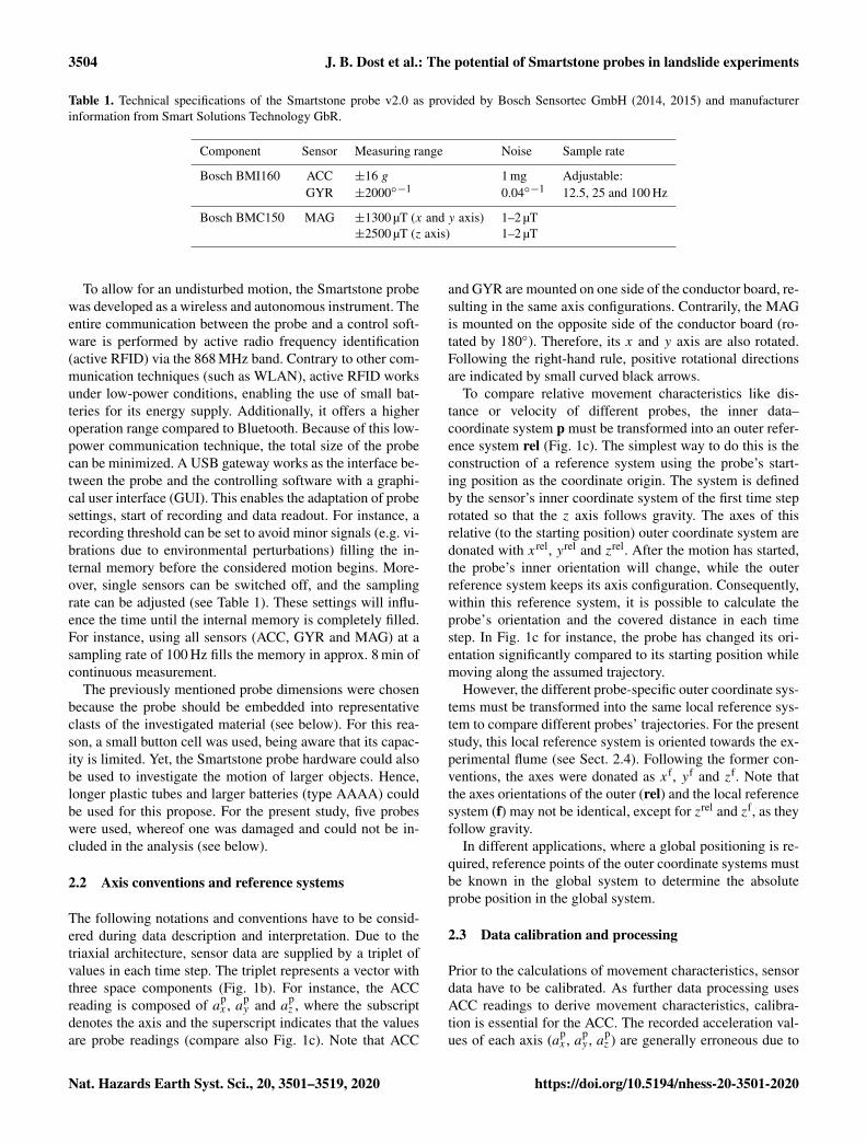
Table 1. Technical specifications of the Smartstone probe v2.0 as provided by Bosch Sensortec GmbH (2014, 2015) and manufacturerinformation from Smart Solutions Technology GbR.

Component Sensor Measuring range Noise Sample rate

Bosch BMI160 ACC ±16 g 1 mg Adjustable:GYR ±2000◦−1 0.04◦−1 12.5, 25 and 100 Hz

Bosch BMC150 MAG ±1300 µT (x and y axis) 1–2 µT±2500 µT (z axis) 1–2 µT

To allow for an undisturbed motion, the Smartstone probewas developed as a wireless and autonomous instrument. Theentire communication between the probe and a control soft-ware is performed by active radio frequency identification(active RFID) via the 868 MHz band. Contrary to other com-munication techniques (such as WLAN), active RFID worksunder low-power conditions, enabling the use of small bat-teries for its energy supply. Additionally, it offers a higheroperation range compared to Bluetooth. Because of this low-power communication technique, the total size of the probecan be minimized. A USB gateway works as the interface be-tween the probe and the controlling software with a graphi-cal user interface (GUI). This enables the adaptation of probesettings, start of recording and data readout. For instance, arecording threshold can be set to avoid minor signals (e.g. vi-brations due to environmental perturbations) filling the in-ternal memory before the considered motion begins. More-over, single sensors can be switched off, and the samplingrate can be adjusted (see Table 1). These settings will influ-ence the time until the internal memory is completely filled.For instance, using all sensors (ACC, GYR and MAG) at asampling rate of 100 Hz fills the memory in approx. 8 min ofcontinuous measurement.

The previously mentioned probe dimensions were chosenbecause the probe should be embedded into representativeclasts of the investigated material (see below). For this rea-son, a small button cell was used, being aware that its capac-ity is limited. Yet, the Smartstone probe hardware could alsobe used to investigate the motion of larger objects. Hence,longer plastic tubes and larger batteries (type AAAA) couldbe used for this propose. For the present study, five probeswere used, whereof one was damaged and could not be in-cluded in the analysis (see below).

2.2 Axis conventions and reference systems

The following notations and conventions have to be consid-ered during data description and interpretation. Due to thetriaxial architecture, sensor data are supplied by a triplet ofvalues in each time step. The triplet represents a vector withthree space components (Fig. 1b). For instance, the ACCreading is composed of ap

x , apy and ap

z , where the subscriptdenotes the axis and the superscript indicates that the valuesare probe readings (compare also Fig. 1c). Note that ACC

and GYR are mounted on one side of the conductor board, re-sulting in the same axis configurations. Contrarily, the MAGis mounted on the opposite side of the conductor board (ro-tated by 180◦). Therefore, its x and y axis are also rotated.Following the right-hand rule, positive rotational directionsare indicated by small curved black arrows.

To compare relative movement characteristics like dis-tance or velocity of different probes, the inner data–coordinate system p must be transformed into an outer refer-ence system rel (Fig. 1c). The simplest way to do this is theconstruction of a reference system using the probe’s start-ing position as the coordinate origin. The system is definedby the sensor’s inner coordinate system of the first time steprotated so that the z axis follows gravity. The axes of thisrelative (to the starting position) outer coordinate system aredonated with xrel, yrel and zrel. After the motion has started,the probe’s inner orientation will change, while the outerreference system keeps its axis configuration. Consequently,within this reference system, it is possible to calculate theprobe’s orientation and the covered distance in each timestep. In Fig. 1c for instance, the probe has changed its ori-entation significantly compared to its starting position whilemoving along the assumed trajectory.

However, the different probe-specific outer coordinate sys-tems must be transformed into the same local reference sys-tem to compare different probes’ trajectories. For the presentstudy, this local reference system is oriented towards the ex-perimental flume (see Sect. 2.4). Following the former con-ventions, the axes were donated as xf, yf and zf. Note thatthe axes orientations of the outer (rel) and the local referencesystem (f) may not be identical, except for zrel and zf, as theyfollow gravity.

In different applications, where a global positioning is re-quired, reference points of the outer coordinate systems mustbe known in the global system to determine the absoluteprobe position in the global system.

2.3 Data calibration and processing

Prior to the calculations of movement characteristics, sensordata have to be calibrated. As further data processing usesACC readings to derive movement characteristics, calibra-tion is essential for the ACC. The recorded acceleration val-ues of each axis (ap

x , apy , ap

z ) are generally erroneous due to



two reasons: (i) a (quasi-)constant misreading, as the mass in-side the sensor, which moves to measure acceleration, is notprecisely equal in all sensors (manufacturing tolerance), re-sulting in a bias as well as a linear scaling of true values, and(ii) the imprecise orthogonal alignment of the sensor axesand crosstalk, meaning that a fraction of each axis acceler-ation will result in readings at the two other axes. Both ofthem can be corrected by adding a sensor- and environment-depending vector (i) to the readings and multiplying themwith a scale factor matrix (ii).

Frosio et al. (2009) describe an optimization algorithmthat estimates these error components simultaneously. In thepresent study this approach was applied for the first timeon Smartstone probe data. Because one probe was somehowdamaged during the experiments, ACC data of the remainingfour probes were calibrated by means of the optimization al-gorithm using MATLAB software. Subsequently, only theseprobes were analysed.

By means of the recorded acceleration and rotation data,the movement characteristics and the probe’s trajectory canbe reconstructed. Basically, these calculations use Newton’sphysical laws and integration of the recorded accelerations.Practically, if the pebble is in motion, gravitational acceler-ation and acceleration due to the motion will interfere. Nev-ertheless, position and orientation in each time step can beestimated by combining the ACC and GYR readings. Thisapproach is termed sensor fusion (e.g. Koch, 2014). In thepresent study a quaternion-based estimation algorithm wasused that was originally developed to track the human gait.It was adapted from Madgwick et al. (2011) and x-io Tech-nologies (2013) and supplies the movement characteristicsvelocity v and displacement s relative to the starting position.Additionally, it enables a 3D visualization of the trajectory.For a detailed description of the computation see Sect. 3.2.

2.4 Experimental setup

The experimental setup was designed regarding the follow-ing requirements: (i) an exact and rapid triggering mecha-nism, (ii) multiple repetitions with identical boundary con-ditions due to homogeneous and dry material, and (iii) flex-ibility for future studies. Figure 2a shows the configurationthat was used for the present study. A spring-based trigger-ing mechanism allowed a rapid release of the material storedin a box on top of the flume. Eight single springs supplieda total spring force of approx. 1660 N. After the release, thematerial moved along an approx. 4.2 m long plane inclinedby 20◦. Some clasts also reached the lower part of the flume,which is inclined by 10◦. Lateral barriers limited the width ofthe flume to approx. 2.2 m. The bottom of the flume was cov-ered by a dimpled sheet to provide uniform basal frictionalconditions.

A high-speed camera was placed close to the storage boxto document the initial motion of the material. A Optro-nis CR4000x2 camera and a Tamron XR Di II (17–55 mm,

1 : 2.8) lens were used. High-speed sequences were recordedat 500 fps (frames per second) with a resolution of 2304×1720 pixels and were stored as ∗.jpeg files. The camera wasmounted with an inclination of 20◦ on the left side of theflume (direction of motion). The recorded pictures were mir-rored during post-processing to achieve a better comparabil-ity between high-speed sequences and probe data. Therefore,motion proceeds from left to right in all attached figures andthe supplementary high-speed video (Video 1). The video fa-cilitates the verification of the interpretation (if the pebble isvisible) of the sensor data and the concluded motion modes.We will refer to it several times.

For the present study, a uniformly graded pebble materialof fluvial origin (fluvial deposit of Moselle river) was used.Lithologically, it mainly consists of quartzite with smallerportions of greasy quartz and slate. Therefore, pebbles arelaminated and rounded to well-rounded shapes. The particlesize range was specified to 32 to 63 mm, and the effective unitweight amounts to 1.55 t m−3 (manufacturer information; EI-DEN, 2017). A median particle diameter d50 of 42 mm anda uniformity coefficient CU of 2.1 was determined by siev-ing analysis. Clasts with diameters >60 mm amount to ap-prox. 12 % (w/w; weight to weight) of the material. A totalmass of approx. 520 kg was used for the present study.

From the material several pebbles were taken to beequipped with Smartstone probes. For this purpose, a holewas drilled through the pebble and modified in the way thata snug fit of the probe was achieved. Therefore, the probecould not move within the hole during the motion process.Additionally, the pebbles were marked and numbered to beeasily identified in the high-speed sequences. The specificunit weight of each prepared pebble was determined by im-mersion weighing before and after the preparation procedure.In this study, a detailed analysis of quarzitic pebble 4 will becarried out. By means of immersion weighing a change indensity (2.66 g cm−3) was not detectable.

The storage box was filled with about 50 % of the materialprior to the experiment. Two probe-equipped pebbles wereplaced, and their position was measured at the temporal sur-face as displayed in Fig. 2b. Afterwards, more pebble mate-rial was filled into the storage box, and three more equippedpebbles were placed at the final surface. Figure 2c and d showthe initial conditions prior to the experiment. The positionsof each equipped pebble were additionally measured relativeto the upper edge of the storage box. This was done usinga laser distance meter (accuracy of ±1 mm). Measures wereconducted for the yf and zf direction for both the starting andthe depositional position.

3 Motion data of landslide experiments and how toread them

Hereinafter, Smartstone probe data of one experiment werechosen to present (i) sensor recordings (Fig. 3), (ii) the de-



Figure 2. Experimental setup. (a) Simplified sketch of the laboratory flume. Green and blue arrows mark axes of the flume reference systemin the yf and zf direction, respectively. (b–d) Starting positions of the five equipped embedded (b) and superficial (c) pebbles. (d) Overlayof (b) and (c) showing the initial positions of all equipped pebbles prior to the experiment. Pebble 4, whose data were plotted in Figs. 3 to 5,is highlighted in light yellow in (b) and (d). Note that pebble 5 could not be included in the analyses due to its damage.

rived movement characteristics (a, v and s, Fig. 4), and(iii) 2D and 3D visualizations (Figs. 5 and 6). The latterillustrate the complex motion trajectory of a single pebblewithin the landslide mass. Subsequently, data of one pebbleare analysed (Sects 3.1 to 3.3) before the motion of multiplepebbles is considered in Sect. 4.1.

3.1 Qualitative description and interpretation of probedata

Figure 3 shows the calibrated data of pebble 4. For this test,only acceleration in g (1 g= 9.81 m s−2, Fig. 3a) and ro-tation in ◦ s−1 (Fig. 3c) were recorded. Note that the threecurves of xp, yp and zp (Fig. 3a) show the acceleration alongthe particular axis (see below). The gyroscope data curves(Fig. 3c) show rotation around these axes. At the top ofeach plot, white bars indicate stationary (no motion) peri-ods, and black bars indicate non-stationary (motion) periods.The previously explained data processing (see Sect. 2.3) wasonly applied to non-stationary periods. The whole motion se-quence can be subdivided into six phases (A to F) with dis-tinct properties characterizing a specific motion behaviour.Additionally, two discrete time points (diamond I and II)indicate major changes within the motion sequence. Thesephases and time markers highlight the same events in Figs. 3to 5 and the supplementary video.

The data sequence of pebble 4 covers a total durationof 2.1 s. The start of motion of pebble 4 was set to 0.0 s.Before the actual motion begins (stationary conditions, leftwhite bars in Fig. 3), low values were recorded along xp

and yp, though xp readings are on a slightly higher level (ap-prox. 0.0 g). At yp, low negative values were recorded. Onlyat zp can higher values of approx. 1 g be seen. This patternrepresents non-motion conditions, where only gravitationalacceleration is recorded. This assumption is supported by thezero readings of the GYR. The plot of Fig. 3b shows thatthe resultant acceleration |a| is approx. 1 g. According to theconventions from Sect. 2.2, |a| can be written as

|a| =

∣∣∣∣∣∣ a

px

apy

apz

∣∣∣∣∣∣=√a2xp + a

2yp + a

2zp = 1g. (1)

Each axis reading reflects a fraction of the gravity vector andis given by

apx = cosα · 1g, a

py = cosβ · 1g, a

pz = cosγ · 1g, (2)

where α, β and γ define the angle between xp, yp, zp and thegravity vector, respectively. Accordingly, under static con-ditions the probe’s orientation relative to the gravity vector(vertical direction) can be calculated from the three readingsof ap

x , apy and ap

z .



Figure 3. Calibrated sensor data of pebble 4. Data are plotted versus relative time since the start of motion. Stationary periods are indicatedby white bars, and motion is indicated by a black bar at the top of each plot, respectively. Vertical bars in light yellow, grey and red markparticular phases (A–F) within the motion sequence (for description see text). Numbered diamonds indicate distinct points in time (see alsoFig. 4). (a) ACC data, (b) resultant acceleration magnitude and (c) GYR data. Curves in (a) and (c) show recordings along and around eachprobe axis, respectively.

3.1.1 Phase A (light-yellow shading)

A sudden change in the axis readings at 0.0 s is visible in allthree plots. Between 0.0 and approx. 0.03 s, a clear drop ofzp recordings to half of the former level is visible in the ac-celeration plot (Fig. 3a). Simultaneously, the values of xp in-crease slightly above zero, and those of yp slightly decrease1.Generally, relatively low acceleration readings are visible onall three axes during phase A, reflected by the resultant ac-celeration (Fig. 3b). Low absolute values of acceleration canonly be achieved if free fall (unconfined acceleration withinthe earth’s gravitational field into the direction of its centreof mass) is mixed with an additional. Thus, values between0 and 1 g imply a hampered free fall (no completely devel-

1The sign of the reading does not imply an increase or decreaseof velocity. A positive value is caused by acceleration along thisaxis; a negative value is caused by acceleration in the opposite di-rection. A positive value as well as a negative value might be due toan increase of the pebble’s velocity or a decrease – depending on itsorientation.

oped free fall, confined motion) and/or an additional lateralacceleration.

In phase A the resultant acceleration is between zero andone. Hence, the pebble moved more or less downwards butwas not in free fall. In fact, it was confined by the surround-ing mass (see below). During phase A, angular velocitiesof about ±250◦ s−1 are visible in Fig. 3c. It is conspicuousthat between 0.0 and approx. 0.2 s, negative values are visi-ble on xp and yp, while zp shows positive values. Betweenapprox. 0.2 and 0.38 s, oppositional axis configurations withlow absolute values at zp and positive angular velocities at xp

and yp are displayed. These features show a forward andbackward rotation of the pebble mainly around xp and yp.Generally, phase A is characterized by relatively smoothcurves without any large peaks and comparably low sensorreadings for both the ACC and the GYR. Thus, it appearsthat during this phase, a relatively calm motion behaviourwas present without any stronger collisions between pebble 4and the surrounding clasts. We conclude that the surroundingpart of the mass moves coherently downwards.



3.1.2 Diamond I and phase B (light-grey shading)

At 0.389 s (diamond I) a distinct transition in the data se-quence is visible. Contrary to phase A, uneven and peakycurves can be seen in all plots. In Fig. 3a, zp generally showshigh acceleration peaks of approx. 3.0 g. Along yp, valuesaround−1 g were recorded; along zp, values around 1 g wererecorded from 0.389 to approx. 0.7 s. The resultant accelera-tion (Fig. 3b) also shows a peaky curve with values between0.2 and approx. 3.0 g. Looking at the GYR data, high an-gular velocities of about 600◦ s−1 at xp and yp are visiblearound diamond I. This indicates a strong rotation aroundthese axes and may be a hint for major changes in direction.After that, relatively low ω values < 500◦ s−1 are recordedduring phase B.

3.1.3 Diamond II and phase C (light-yellow shading)

At diamond II another strong transition is visible in thetime series. The strongest peak of the whole sequence (ap-prox. 4.6 g) is measured at zp for two subsequent read-ings. Thus, the change in velocity is bigger than all otherchanges, as the strongest absolute acceleration also lastslonger than most other acceleration peaks, which only con-sist of one reading. Because of the low acceleration record-ings of xp and yp, the resultant acceleration is calculated toapprox. 4.7 g. Diamond II introduces phase C, where highersensor reading in GYR data are visible as well (Fig. 3c).Here, the phase begins with a relatively low ω value of ap-prox. 260◦ s−1 at 0.898 s on yp. After that, a strong increaseon yp is visible until at 0.918 s, a local maximum of approx.1230◦ s−1, is reached. Interestingly, this peak was recordedafter high values were recognized at ap

z , 0.01 s earlier. Whilethe GYR readings of xp and zp are relatively low at ap-prox. −150◦ s−1, values of yp stay at a high level of ap-prox. 750◦ s−1. At the end of phase C, an increase of ω at yp

is visible.These recordings can be interpreted in the way that peb-

ble 4 changes its mode from lateral sliding to rotation andsaltation. This point in time is also clearly visible in Video 1at the position marked with diamond II. In the following,each saltation is characterized by single strong peaks on dif-ferent axes (as the pebble also rotates).

3.1.4 Phase D (light-red shading)

The short period between 1.008 and 1.038 s (four data sam-ples) can be easily identified within the acceleration plots(Fig. 3a and b). Low ACC readings of all three probe axesled to a resultant a close to zero. As explained above, this isonly possible under almost free-fall conditions. Therefore, itcan be reasoned that the pebble 4 fell for approx. 0.03 s. Thegyroscope plot (Fig. 3c) shows again high values of approx.900◦ s−1 for yp and relatively low values for xp and zp. Thisimplies a pronounced rotation while the pebble falls.

3.1.5 Phase E (light-yellow shading)

A strong rotation around yp continues at the beginningof phase E. But contrary to the former phases, ωp

x andω

pz show increasing positive and negative values since ap-

prox. 1.07 s, respectively. At approx. 1.14 s a peak of ω ofapprox. −820◦ s−1 occurs at zp before the values decreaseagain. At about the same point in time, strong peaks are visi-ble at the ACC readings at each probe axis. These lead to thesecond highest a resultant (approx. 4.2 g) of the whole timeseries. From approx. 1.23 to approx. 1.24 s another short pe-riod of ACC readings around zero is visible, resulting in ana resultant of approx. 0 g. At the end of phase E, a last stronga peak (3.6 g) at zp and a strong decline of the ωp

y are visible.This denotes a major change in motion behaviour with a tran-sition from strong rotations in phases C to E to less rotationalbut translational displacement.

3.1.6 Phase F (light grey) and the end of motion

During this last phase, a continuous decline of ω at all probeaxes can be seen. Whereas values of approx. ±200◦ s−1 arerecorded at approx. 1.3 s, until the end of the movement analmost logarithmic decrease of these values is visible. Thisdecline appears also at the ACC readings from approx. 1.53 sonwards. At 1.826 s the end of the motion sequence isreached. GYR readings around 0◦ s−1 were recorded. At theACC, only minor changes can be seen after this point in time.At zp values vary slightly below 1 g. Readings of xp and yp

are slightly higher than 0 g. As the pebble is stationary, onlythe gravitational acceleration vector is displayed by the data.This is also visible in Fig. 3b, where the calculated a magni-tude varies around 1 g.

Concerning the whole time series, some interesting as-pects shall be mentioned: the small deviations from the meanaxis readings of the ACC after the motion (right white bar)can be interpreted as oscillation of the flume construction af-ter the impact. This is supported by the data pattern exhibit-ing uniform oscillations which are gradually decreasing inamplitude.

By comparing the ACC readings before and after themovement (white bars), a minor change of xp and yp canbe seen. While xp showed values of ±0.0 g and slightlynegative readings of yp before the start, low positive val-ues were recorded after the motion on both axes. Contraryto this, zp shows slightly lower values after the motion com-pared to its readings before the start of the experiment. Fromthis can be reasoned that the orientation of pebble 4 after themovement has changed. Because the stationary ACC read-ings of zp are slightly lower, it follows that this axis does notpoint exactly in the vertical direction after the motion. Theprobe is oriented in a different way than prior to the experi-ment.

Further, different “modes” of sensor readings occur duringthe motion sequence. The first mode is generally character-



ized by little ACC readings on all axes. In addition, the curvesare relatively smooth and less peaky, which is particularlyclear for the rotation data. This mode is present in phase Aand for the short period of phase D. The second mode con-sists of peaky and relatively high acceleration values simul-taneously with relatively low but peaky GYR readings. Theamplitude of ACC values is relatively high. This mode oc-curs during phases B and F. Contrary, a third mode showssmoother (less peaky) ACC readings with lower amplitudesand high but less peaky GYR recordings. This mode can beobserved in phases C and E. These oppositional observa-tions reflect the previously mentioned motion behaviour. Thefirst mode is recorded when the pebble mainly falls down-wards and clast contact is inhibited. The second mode isrecorded if translational transport under confined conditionsoccurs. Pebble 4 moves within the mass and is exposed topronounced collisional contacts due to surrounding pebbles.This results in frequent impacts and, consequently, accelera-tion peaks. Because the pebble is generally not free to move,larger rotation is inhibited and minor but sudden orienta-tion changes occur. This is reflected by the relatively low butpeaky GYR readings. Contrary, the third mode occurs whenthe pebble rotates unconfined. This is only possible while thepebble is not surrounded by other material. This means thatthe pebble must be above the moving mass. In other wordsand geoscientifically speaking: the pebble saltates. This isalso supported by the alternating pattern of high peaks andalmost zero acceleration magnitude. This pattern results fromsaltation as the pebble bounces at the flume bottom before itrebounds and falls again.

3.2 Quantifying motion by means of derived movementcharacteristics

The previously explained data only focussed on the motionmode. In the following, the movement is investigated withrespect to position and time. The recorded data are only aresult of external influences (forces) that act on the pebble.However, from the recorded and calibrated data, the peb-ble’s movement characteristics relative to its staring position(arel, vrel and srel) can be derived by simple physical rela-tions. The initial orientation of the pebble can be calculatedaccording to Eqs. (1) and (2). By means of the received Eu-ler angles α, β and γ , the sensor readings ap

x , apy and ap

z canbe rearranged to arel

x , arely and arel

z (compare also Sect. 2.2).However, the representation by Euler angles may not be bi-jective and therefore may lead to an erroneous initial orien-tation (“gimbal lock”). Another method to derive initial ori-entation by means of acceleration and rotation data was pre-sented by Madgwick et al. (2011). It is based on a quaternionrepresentation and supplies bijective solutions (for detailedexplanations the reader is referred to Madgwick et al. (2011)and specific literature such as e.g. Jazar, 2011). It was imple-mented into a MATLAB algorithm, which was published on-

line at https://x-io.co.uk/gait-tracking-with-x-imu/ (last ac-cess: 3 August 2017) (CC license; x-io Technologies, 2013).

After finding the initial orientation, the vector arel con-sequently gives the translational acceleration of the pebblewithin a reference system relative to the pebble’s staringposition (compare Fig. 1c). Thereby, the direction of arel

z

equals the gravity vector and thus points downwards. Hence,arelx and arel

y give the horizontal component of arel. After therearrangement of the recorded accelerations and with respectto time t , the movement characteristics vrel and srel can beobtained from the integration as

vrel(t)=

∫arel(t)dt (3)

and

srel(t)=

∫vrel(t)dt. (4)

By applying these formula, movement characteristics werecalculated for the non-stationary period and are plotted inFig. 4a–c. Individual phases and distinct points in time are in-dicated in the same way as displayed in Fig. 3. Additionally,captures of the high-speed sequence from diamonds I and IIare shown in Fig. 4d. Note also that acceleration values areplotted in units of m s−2. Data processing was applied fromthe start of motion (compare black bars in Figs. 3 to 5). Onlyarel was rearranged before the motion starts (white bars).During stationary periods these values are defective. This canbe seen at xrel (Fig. 3a), where values of approx. −4 m s−2

were calculated. Obviously, this cannot be true as the peb-ble does not move. However, these false calculations are ex-cluded from further integration (compare Fig. 3b and c) anddo not influence the following interpretations. A summary ofthe finally derived distances that were covered by pebble 4during each phase is listed in Table 2.

Relatively low acceleration values are calculated dur-ing phase A. As displayed in Fig. 4a, arel

z generally in-creases until at approx. 0.32 s a local maximum of ap-prox. −9.4 m s−2 occurs. This is less than gravitational ac-celeration (9.81 m s−2). Therefore, it can be reasoned thatfree-fall conditions were not totally developed during thisphase. In fact, pebble 4 was confined by the underlying mass.This can also be seen in Fig. 4d, where pebble 4 “swims” atthe surface of the moving material. Therefore, phase A couldbe termed as “confined fall”. The highest derived velocityof vrel

z during phase A was calculated at approx. 1.7 m s−1 at0.379 s. Afterwards the vrel

z velocity component decreased.Simultaneously, the vrel

y velocity component increased fur-ther. During phase A, a cumulated vertical distance of ap-prox. 0.35 m was covered. The srel

y component amounts toapprox. 0.18 m at the end of phase A (see Table 2).

At 0.389 s after the start, a discontinuity on the x andz axes is visible in Fig. 4a and b. The corresponding cap-ture of the high-speed sequence is shown in Fig. 4d. Thevariability of the acceleration time series increases. This


https://x-io.co.uk/gait-tracking-with-x-imu/


Figure 4. Movement characteristics and high-speed captures. (a–c) Time series of the derived movement characteristics for (a) translationalacceleration, (b) translational velocity and (c) translational displacement (with detail). The three curves in each plot give calculated time-dependent values for each axis of the relative reference system (as defined in Sect. 2.2). Motion phases and distinct time points are indicatedas in Fig. 3. In (c) green and blue dots indicate the true displacement components in yf and zf directions measured by means of a laserdistance meter (for explanation see Sect. 2.2). (d) High-speed captures at time points diamond I and II. The data of (a–c) were recorded withpebble 4, which is highlighted in light yellow and labelled in (d).

Table 2. Motion phases of pebble 4 as displayed in Figs. 3–5 and high-speed video. IDX gives the index of data samples, and tStart gives thetime in seconds since the start of motion. Frame is indicated by the frame number as displayed in Video 1. For other columns see descriptionwithin the text.

Phase IDX tstart Frame srely srel

z sfy sf

y

[–] [s] [–] [m] [m] [m] [m]

A 12 0.000 64 0.000 0.000 – –B 51 0.389 259 0.1774 −0.3464 – –C 102 0.898 513 0.7823 −0.7955 – –D 113 1.008 568 0.8739 −0.8094 – –E 116 1.038 583 0.8958 −0.8217 – –F 143 1.307 718 1.0957 −0.9326 – –End 195 1.826 977 1.2962 −0.9988 1.4240 −1.1090



was already identified in Fig. 3. A first strong peak of ap-prox. 14.7 m s−2 occurred at arel

z and marks the beginningof phase B. At this time, a transition from confined fall totranslational movement occurs. Additionally, the peaky pat-tern of the acceleration and velocity curves indicates pro-nounced clast contact and energy dissipation. This is particu-larly clear for vrel

z . Because pebble 4 moves at the surface ofthe material, clast contact occurs mainly in the vertical direc-tion. During phase B, the vertical velocity component subse-quently decreases. Meanwhile, vrel

y increases until at 0.609 sthe maximum of approx. 1.45 m s−1 is reached.

Phase C again is introduced by a sudden strong increasein arel

z at 0.898 s (diamond II). The acceleration peak at0.908 s of approx. 35.9 m s−2 leads to a positive vertical ve-locity of approx. 0.21 m s−1. The pebble consequently movesupwards at this point in time, which can be seen in thedisplacement plot (Fig. 4c). Afterwards, the displacementtends again to downward motion in phases D and E. Duringphases C to E, the displacement plot (Fig. 4c) shows stair-like features at the srel

x and srelz curves. These features can

only be achieved if the actual motion acts against the ten-dency of downward movement parallel to the flume bottom(see Fig. 1). Together with the previously mentioned high ωaround all probe axes (compare Fig. 3), a complex rotational-motion pattern can be interpreted until 1.307 s. Note that onlythe first milliseconds of this complex motion are visible inVideo 1, since pebble 4 left the field of view at approx. 1.0 s.

In phase F, the components of translational accelerationand derived velocity gradually decline, which leads to onlylittle displacements. A total displacement of approx. 1.0 m inthe zrel direction and 1.3 m in the yrel direction was calcu-lated by means of the formerly mentioned algorithm. Addi-tionally, in Fig. 4c the covered distance measured with a laserdistance meter in the flume direction is plotted. Although be-ing aware that yrel and yf do not necessarily have to be identi-cal (compare Fig. 1 and Sect. 2.2), a high agreement betweensensor-derived and manually measured displacements is dis-played. It can be reasoned that the probe must be orientedmore or less in the flume direction, following that the probeaxes xrel and yrel approximate xf and yf. As the vertical di-rection is derived from ACC readings under stationary con-ditions, zrel equals zf. Thus, the deviation between srel

z and sfz

reflects the quality of the sensor-derived position. Whereas asensor-derived vertical displacement of 0.999 m was calcu-lated, a true vertical displacement of 1.109 m was measuredin fact (see Table 2). This means the calculations underesti-mate the vertical displacement by less than 10 %.

3.3 Visualizing motion by trajectory reconstructions

As described in Sect. 1, high-speed video recording is oneof the traditional methods to observe rapid movements. Sucha video sequence was recorded for the present study as well(Video 1). Due to narrow conditions at the experimental fa-cility, the high-speed camera had to be installed very close

to the setup, resulting in a relatively small field of view. Atthe end of the high-speed sequence, nevertheless the start ofa complex rotational motion of pebble 4 can be observed.However, the full motion feature is not visible.

Although only the first portion of this complex motion isvisible on the high-speed sequence, the full trajectory can bereconstructed by means of the recorded Smartstone data. Thetrajectory is defined as the position vector composed of srel

x ,srely and srel

z for each time step (Fig. 4c). As additional in-formation, the pebble’s orientation can be reconstructed bymeans of the previously described algorithm. Consequently,these variables can be plotted as a function of time within aCartesian coordinate system, as displayed in Fig. 5. Thereby,the axes xrel, yrel and zrel denote the distance axes relativeto the starting position of the pebble. Note that zrel alwayspoints in the vertical direction (for explanation see above)and that diagram axes of Fig. 5 are not drawn to the samescale. Note further that contrary to Figs. 3 and 4, Fig. 5 showsno time series but visualizes the pebble’s position within therelative reference system.

In Fig. 5a, the trajectory projected on the yrelzrel plane canbe seen, displayed in the same orientation as in Video 1. Ad-ditionally to the side view perspective, data can also be visu-alized from a top view, where the trajectory is projected onthe xrelyrel plane (Fig. 5b). Moreover, the 3D trajectory canbe visualized as displayed in Fig. 5c. The pebble’s position ismarked by small black dots, and the probe’s axes are shownin red (xp), green (yp) and blue (zp), indicating its orienta-tion at each position. Note that the axes are smaller if theypoint towards the viewer or the opposite (off the displayedplane). Positions (black dots) are plotted with a constant fre-quency, which was reduced to 1

3 of the recording frequencyof 100 Hz, for reasons of clarity.

On the side view plot (Fig. 5a), yp and zp are almost drawnin full length, whereas xp is short, indicating its orientationtowards the viewer’s perspective. It can be reasoned that thepebble is oriented almost horizontally before the motion be-gins. By comparing the three plots of Fig. 5, one can observethat the probe is slightly tilted around the yp axis towards theleft side.

During phase A, mainly vertical displacement can be seenin Fig. 5a. Projected on the yrelzrel plane, the trajectory showsan almost linear pattern. On the xrelyrel plane (Fig. 5b), aslight rightward displacement is visible. The pebble’s orien-tation remains more or less constant, and only minor tiltingcan be observed as the yp axis (green) points a little down-wards. At the end of phase A, the pebble rotates back again.

In phase B, a transition to a curved trajectory can be ob-served in Fig. 5a. Interestingly, a major change in the move-ment direction emerges on the top view at diamond I as well(Fig. 5b). Whereas the pebble moves slightly to the left dur-ing phase A, a change in the movement direction towards theright is induced at this point in time. Additionally, a slowrotation of the pebble can be observed in phase B mainlyaround the yp axis. This rotation contains portions around



Figure 5. Visualization of the reconstructed trajectory within the relative reference system. Red, green and blue coloured lines indicateprobe axes and display its orientation within the relative reference system as defined in Sect. 2.2. Motion phases and distinct time points areindicated as in Fig. 3. (a) 2D side view (yrelzrel plane), (b) 2D top view (xrelyrel plane) and (c) 3D perspective view. The dashed grey linerepresents the tilted flume for illustration.

the other axes as well. Note also that from the beginningof phase A to about the middle of phase B (approx. 0.5 mon yrel), the distance between the small black dots (indi-cating its position) increases, indicating increasing velocitygiven a constant rate of displaying the position (33.3 Hz, seeabove). Afterwards, the distance between the position pointsdecreases, resulting from the deceleration of the pebble.

At diamond II, a major transition was identified abovefor both probe data and movement characteristics. The sametransition is obvious in Fig. 5 as well. While axis configura-tions only varied slightly during phases A and B, pronouncedchanges can be seen during phases C to E. The whole com-plexity of the rotation in these phases can be recognized bycomparing the three plots of Fig. 5. It is visible that the peb-ble rotates around all axes. Further, the distances betweensingle black dots increases again, implying repeated accel-eration. Although these rotations were not completely doc-umented by the high-speed sequence (Video 1), the recon-structed 2D and 3D trajectories reveal the complex rotationthat was induced by a sudden impact at diamond II (comparealso Figs. 3 and 4).

Phase F is again characterized by relatively small but con-tinuous changes in axes orientations and by an almost lineartrajectory pattern. The distances between the black dots de-crease further, reflecting the decreasing velocity. In addition,Fig. 5 shows that the pebble’s orientation at the end of motiondiffers significantly from its starting orientation. The pebbleis strongly rotated as the xp and yp axes point towards thestarting position. This could not be identified in the probedata plotted in Fig. 3. Here, only little changes in ACC read-ings were identifiable. This reflects critical states, where dif-ferent orientations lead to similar (or equal) axis readings.

To derive the correct orientation, advanced techniques haveto be used, like a quaternion-based approach (compare e.g.Hanson, 2006). Apart from that, the zp axis points – slightlytilted – in an upward direction. Note also that the flume bot-tom is inclined by 20◦ (compare Fig. 2). Therefore, the lineartrajectory reflects parallel motion along the flume bottom.

4 Potentials and limitations of the Smartstone probe

4.1 Trajectories of multiple pebbles in one experiment

A detailed analysis of the reconstructed motion behaviour ofa single clast within a moving mass was given above. Be-yond that, three more pebbles were equipped with Smart-stone probes in the same experiment, and their trajectoriescould be reconstructed in the same way as for pebble 4. Con-sequently, the four trajectories can be plotted together withinone diagram providing that a higher-ordered reference sys-tem is applied (see Sect. 2.2 and Fig. 1).

Figure 6 shows the reconstructed spatiotemporal trajecto-ries of four pebbles that were equipped with a probe. Notethat vertical and horizontal axes of the diagram are drawn onsame scale, and the duration is colour-coded relative to thestart of movement. Additionally, time stamps are displayedat 0.25, 0.5, 1.0 and 1.5 s for each trajectory, respectively.The first motion of the four analysed pebbles was set to 0.0 s(pebble 1). Therefore, both time and position coordinates dif-fer from Figs. 3 and 5. Thick grey lines give the dimensionsof the flume construction including the storage box with thesimplified material body prior to the start. It is visible thatpebble 1 and 2 were embedded into the material, whereas



pebble 3 and 4 were placed at the surface of the material (seeFig. 2).

Looking at the four trajectories, it can be seen that thepath of pebble 3 falls remarkably steeper than the others.This results in a reconstructed depositional position that isbelow the flume bottom. Here, the reconstruction obviouslyproduces erroneous results. Comparing the end of the trajec-tory and the true deposition of pebble 3, the overall length(projected length of the 2D displacement on yfzf plane) fitsquite well to the measured one. It seems that only the incli-nation of the reconstructed trajectory was wrongly estimatedby the algorithm. A wrong estimation of the initial orienta-tion is considered to be the main disturbance for the wrongorientation of the trajectory. A false reconstruction might oc-cur if the probe did not record the stationary conditions priorto the start of motion. However, the time series of pebble 3was found to be complete after a detailed review. Anotherreason could be that – contrary to the other clasts – pebble 3might be strongly inclined under stationary conditions priorto the start of the experiment. This would result in a wrongestimation of the vertical direction leading to an overestima-tion of the vertical-acceleration component and the double-integrated vertical displacement.

The other trajectories on the other hand show patterns thatare reasonable compared to the reference measurements: thetwo embedded pebbles covered a shorter distance than thepebble placed at the surface. Additionally, at the same pointin time – for instance at approx. 1.0 s since the start of theexperiment (again red coloured) – pebble 4 has travelled ap-prox. 0.4 m further than the embedded ones. Whereas Okuraet al. (2000) observed that blocks positioned at the front werealso deposited in the distal zone, the top pebbles travelled thelongest distance in our experiment. Regarding the high-speedvideo, the explanation is given by the tilted gate: the pebblespositioned on the top start their movement both downwardsand to the right (from the camera perspective), thus not trans-ferring energy to material formerly placed underneath in thestorage box. The higher the pebbles are placed, the biggertheir overhang is, resulting in less material vertically under-neath. Compared to the uniform initiation (multiple blocksslid coherently) of the motion in Okura et al. (2000), less en-ergy dissipation occurs in our experiment.

Moreover, the embedded pebble 1 displaced roughly 70 %of the resulting distance (approx. 0.35 m of 0.50 m) withinapprox. 0.5 s (light-blue colours). It is conspicuous that dur-ing this phase mainly vertical displacement occurs, whereasfor the latter 30 % of its trajectory it moves more or lessparallel to the inclined flume plane. For this part of its tra-jectory the pebble needs another approx. 0.8 s until it finallydeposits. It can be reasoned that a strong gradient in veloc-ity magnitude after the transition from mainly vertical to lat-eral displacement occurs. This motion behaviour was onlyobserved for pebble 1 in this experiment. Contrary to peb-ble 1, the trajectory of pebble 2, which was embedded aswell, shows a uniform pattern. In addition, a smooth velocity

gradient can be observed, indicated by gradually changingcolours. Therefore, the two pebbles, which were embeddedat opposite sides of the material (compare Fig. 2), show dis-similar motion patterns. Probably the motion behaviour de-pends on the pebble’s distance to the opening board of theflume. Clasts that are further to it – such as pebble 2 – are sur-rounded by more material confining a free motion. Therefore,almost free-fall conditions will be easier to achieve closer tothe opening as in the case of pebble 1. This is also in agree-ment with the reconstructed trajectory of pebble 4 that showsa similar pattern until approx. 1 s after the start.

Contrary to the uniform trajectories of pebbles 1 and 2,saltation can be recognized approx. 1.15 s after the start be-tween approx. 1.3 and 1.6 m horizontal distance (yf) for peb-ble 4. This feature is the result of the complex rotations thatwere identified in probe data (Fig. 3) as well as the derivedmovement characteristics (Fig. 4) and were finally visual-ized in Fig. 5. Now, comparing all valid trajectories withinthe flume reference system, this bumping pattern of pebble 4becomes very notable. During this phase the general lateralmotion along the inclining plane – driven by gravitationalacceleration and decelerated by friction – is interrupted. Infact, the pebble moves more or less horizontally before itfalls again and proceeds its “normal” motion. This extraor-dinary motion pattern was initiated by a strong hit visible inthe probe motion data (Fig. 3a) at diamond II. Although thetrigger can be identified in the probe data, its actual meaningand, subsequently, a suitable interpretation is only possibleif the movement is visualized within the correct spatiotem-poral context. Hence, a rudimentary plotting of probe datais not sufficient to describe and interpret geomorphic move-ment processes adequately.

4.2 Probe restrictions and analytical limitations

The current Smartstone probe v2.0 exhibits one main draw-back. Since the probe development focussed on the minimalpossible size, only a small button cell battery can be used asits energy supply. This means that battery life is restricted, es-pecially under cold conditions. This resulted in pronouncedbattery wastage. During the future development of the Smart-stone probe, alternative options for energy supply will haveto be evaluated.

Beyond the battery issues, some probes seemed to beerror-prone. As indicated before, it was not possible to recorda calibration sequence with one probe. Although this probewas handled in the same way as all others, it was somehowdamaged. In this case, an initiation of the recording modewas not possible anymore. The reason for this could not beevaluated.

Despite this, all other probes could be used during the ex-periments, and the data could be used to reconstruct the 3Dtrajectories as described above. When comparing the end ofeach valid trajectory and the true depositional position, a par-ticular deviation of several centimetres is visible. In all cases



Figure 6. Reconstructed spatiotemporal trajectories and true depositional positions of four pebbles within the local flume reference system.2D side view (yrelzrel plane). In addition, the idealized flume construction and the pebble material body prior to the experiment are drawn inlight-grey colours. Note that the equipped pebbles are not drawn to scale due to clearness reasons. The trajectories are colour-coded, wherethe colour represents the relative time since the start of the experiment (first motion, pebble 1). Additionally, specific points in time arehighlighted by time stamps.

the reconstructed trajectory is shorter than the actual distancethat was covered by the pebble. It can be reasoned that thedisplacement is generally underestimated by the calculations.This is in contrast to the analytical results of Gronz et al.(2016), where mainly the clipping of ACC readings led toan overestimation of the displacement. In the present exper-iment, clipping was not observed due to the enhancement ofthe ACC recording range.

Another explanation for an erroneous displacement deriva-tion might be an incorrect duration of the non-stationary pe-riod. During data analysis, the beginning and end of the non-stationary period were set manually, since the primary fil-ter approach of x-io Technologies (2013) was not applica-ble for these kinds of motion processes. As described be-fore, the algorithm was originally developed to track the hu-man gait that is characterized by uniform and distinct mo-tion patterns. Since the motion behaviour of clasts within amoving granular material possesses a higher level of com-plexity and is less predictable, the necessary filter parametersettings change significantly for each recorded motion. Con-sequently, for each pebble and in each experiment, multiplefilter parameters would have to be found. Therefore, a man-ual setting was considered to be more effective. Since thestart of the motion process is clearly visible in the sensor

data (compare Fig. 3), the beginning of the non-stationaryperiod can be set easily. On the other hand, the motion pro-cess mostly declines gradually and slowly (compare Sect. 3.1and 3.2). Therefore, the end of motion was difficult to iden-tify. In a consistent way, the end of non-stationary periodswas set to a time step, where almost no rotation was recordedby the GYR. Around this time at the end of the recordedsequences, ACC readings were low as well. This indicatesthat more or less only gravitational acceleration was actingon the pebble, and acceleration due to transport motion wasnegligible. Therefore, it is unlikely that a further transport ofthe pebble and, consequently, an unrecognized displacementoccur. Accordingly, somewhat shorter or longer durations atlow acceleration magnitudes do not significantly influencethe derivation of displacement. Although the manual defini-tion of the end of motion will always be debatable, the effectof a slightly longer or shorter motion is considered to be ex-tremely small.

Other explanations for the deviation between true and cal-culated distances are (i) errors due to integration and (ii) im-precise estimations of the probe’s orientations. Besides oth-ers, these errors were discussed in detail by Gronz et al.(2016). Because the probe data have a finite sampling rateand resolution is integrated twice in each time step, a devia-



tion will always occur and will increase with both time andcovered distance.

In the present study, the deviation is considered to bemainly caused by imprecise orientation estimations. As de-ducted by Gronz et al. (2016), an orientation error of only1◦ will lead to an erogenous displacement of approx. 0.34 mafter 2 s of motion. Compared to the former experimentsof Gronz et al. (2016), MAG data were not recorded andcould therefore not be included into the sensor fusion anal-ysis. Keeping this in mind, a deviation between true andreconstructed displacement of approx. 10 % (pebble 4, seeSect. 3.2) demonstrates a good quality of the applied method-ology. Especially the avoidance of clipping errors contributesto this promising result. This was achieved by enhancing theACC measuring range from ±4 to ±16 g (compare Gronzet al., 2016).

4.3 Possible ways to enhance the probe accuracy

A comparable low deviation was achieved by merging onlyACC and GYR data. Therefore, it can be reasoned that afurther enhancement would be possible with the inclusionof MAG data. This would also allow for displaying the tra-jectory in a global reference system. The effect of these en-hancements will be within the scope of further studies.

A further accuracy enhancement of the trajectory recon-structions could be achieved by applying methods that arewell-established in different disciplines like pedestrian nav-igation or mobile robotics, like Kalman filtering or Markovlocalization. The latter approach uses a probabilistic descrip-tion of the possible position of the pebble as a density field,which is updated in the upcoming time step(s) (Fox et al.,1999). Not only probe data but also information about thesurrounding relief (flume geometry) could be used, for in-stance. Additionally, information about the pebble (e.g. ge-ometry and specific unit weight) or the surrounding materialcould be implemented. Further studies will have to evalu-ate which of these pieces of information will lead to an evenbetter reconstruction of the trajectory. Another aspect worthmentioning might be the automatic indication of the motionmode like that proposed by Becker et al. (2015).

4.4 Scaling

A scaling of the recording ranges will be necessary if theSmartstone method is adapted to other experimental scales orvelocities. Additionally, the scaling of temporal persistenceof movements has to be respected, as the Nyquist frequencyto observe the motion without undersampling changes withthe rate of movement changes (Yang et al., 2009). This meansthat a small pebble in a fast-moving landslide will show moreabrupt changes in its velocity, trajectory and mode than alarge block in a slow landslide. Thus, the ranges of the sen-sors and the sampling frequency have to be adjusted depend-ing on the landslide velocity and the particle size. Several

aspects concerning the sensor recording range for differentexperimental applications have to be considered.

– Acceleration range. The expected acceleration dependson the velocity of the landslide, as the strongest peaksoccur during non-elastic collisions of moving parti-cles with stationary boundaries, e.g. bedrock. Thus, therange needs to be increased (by choosing a different ac-celerometer chip in the Smartstone) with velocity. How-ever, to choose a gratuitously large range to avoid clip-ping is counterproductive, as the quantization error willalso increase because there is only a limited number ofsteps within the range. A deliberated balance needs tobe chosen, e.g. by performing preliminary tests.

– Gyroscope range. The rotational velocity depends notonly on the movement of the landslide but also on thesize of particles. For instance, if the mass moves at1 m s−1, a single rolling pebble with a 30 mm diame-ter will show a rotational velocity of 3820◦ s−1 (pebblecircumference of 942 mm, thus 10.6 rotations per sec-ond). Thus, the expected range can be calculated us-ing the shortest circumference of the host particle ofthe Smartstone(s) and the expected landslide velocity.Again, choosing a gratuitously large range to avoid clip-ping will increase the quantization error.

4.5 Potentials of the Smartstone probe

Although the exact depositional position could not be recon-structed quantitatively, which is particularly pronounced forpebble 4, qualitative depositional features were found cor-rectly. For instance, pebbles 1 and 2 were embedded beforeand were also within the deposit after the experiment. Thiscan be concluded from the relatively large vertical distancebetween the end of trajectory and the flume plane. Contraryto that, pebble 4 was originally deposed directly at the in-clined plane which is also reproduced by means of probedata.

Furthermore, the complex rotational movement of peb-ble 4 can be identified in the reconstructed 3D trajectory.This particular feature becomes also clear if one comparesthe trajectory of pebble 4 with the other reconstructed trans-port paths (see above and Fig. 6). Contrary to pebble 4, theother clasts follow relatively simple trajectories. This can beexplained by the position of these clasts embedded within thebody. Therefore, the motion was strongly confined. Althoughonly data of four probes could be analysed, prominent differ-ences of the motion behaviour dependent on different posi-tions within the moving mass could be found.

These results demonstrate the potential of using in situ mo-tion sensors to characterize artificial landslide movements.Contrary to external-observation methods, such as high-speed videos or laser techniques (e.g. Manzella and Labi-ouse, 2009), the internal measurement supplies continuousmovement characteristics for a single particle in 3D space.



The Smartstone probe thereby overcomes the issue of con-fining the motion process by wires. This problem emergedin many experimental studies that tried to measure the inter-nal deformation or movement characteristics (e.g. Moriwakiet al., 2004; Ochiai et al., 2004, 2007; Olinde and Johnson,2015). Although the influence due to wired sensors seemssmall, its exact effect on the motion process cannot be de-termined. By means of unwired sensors this methodologicalinaccuracy can be avoided.

In the future, Smartstone probes may help to explain ob-servations from the modelling of landslide motion processes.For instance, it would be interesting to investigate the influ-ence of clasts with different sizes. Phillips et al. (2006) ob-served a uniform distribution of fine and coarse particles inlaboratory high-mobility granular flows. Providing the rightscale (compare Sect. 4.4), trajectory reconstruction of differ-ent clasts may shed light on the question about how differentclast sizes segregate during the transport process. A deeperanalysis of the probe data may also allow for estimations ofenergy dissipation within the landslide body during the mo-tion process (compare e.g. Manzella and Labiouse, 2013).

Beyond these geoscientific objectives, the Smartstoneprobe was successfully used in experiments focussing oncoastal-engineering and hydro-engineering problems. Santoset al. (2019) briefly reported experiments to investigate thestability of breakwater amour units. By means of the Smart-stone probe data, Ravindra et al. (2020) presented a detailedanalysis of the failure mechanism of placed riprap on labo-ratory dam models. These examples demonstrate the broadapplicability of the Smartstone technique.

During the last years, both wired and unwired sensors(IMU or other combinations of ACC, GYR and MAG) wereused to observe geomorphic-motion transport processes. Ooiet al. (2014, 2016) for instance used it to study the initia-tion process of small-scale laboratory landslides. They usedthe ACC data for qualitative interpretations concerning thetiming of landslide initiation. Additionally, they interpreted arotational failure process from changing vectorial portions ofthe gravity vector on different axes. Nevertheless, a quan-titative characterization was not carried out. The potentialof recording motion data of geomorphic movements is farbeyond a simple plotting of probe data. In fact, it allowsfor the sampling of movement characteristics. Therefore, therecording and analysis of geomorphic-motion data expandthe toolkit of landslide science.

Recently, Spreitzer et al. (2019) used an approach sim-ilar to that in the present study to derive Euler angles ofmoving wood in laboratory experiences. They illustrate thesuitability of this technique to characterize certain transportfeatures. Beyond the derivation of Euler angles, the presentstudy demonstrates that the calculation of movement charac-teristics and the reconstruction of spatiotemporal trajectoriesare essential to describe geomorphic-motion processes ade-quately.

These derivations are possible even if only accelerationand rotation data are recorded by means of a 6-DoF (degreesof freedom) probe. Further, a full 3D reconstruction of mul-tiple trajectories was achieved. This allows for a comparisonbetween different parts of the moving mass. Accordingly, thepresent study demonstrates that the “sampling of motion”ofsingle stone movements is possible.

5 Conclusions and final remarks

Laboratory experiments are a common tool to study land-slide processes in detail. However, a critical – but also diffi-cult – task is to capture the internal dynamics of the movingmaterial. In the present paper, we presented the autonomousSmartstone probe v2.0 that is able to measure in situ motiondata of single clasts moving embedded or superficially in/ona landslide mass. The main conclusions of the present studycan be summarized as follows:

– The Smartstone probe in its recent version fulfils all re-quirements to use it as an additional tool to capture sin-gle clast movements in laboratory-scale artificial land-slides. Especially its size and measuring range satisfythe development aims. Additionally, the probe dimen-sions are adaptable to other experimental conditions orresearch objectives. The Smartstone probe can be usedunder dry and wet conditions and is able to move, recordand transmit data autonomously and wirelessly. Thecommunication works under low-power conditions viaactive RFID (contrary to the high-power conditions ofWLAN).

– Already the calibrated probe data offer broad insightsinto the motion process. By means of the accelerationand rotation time series the motion sequence of peb-ble 4 could be subdivided into six phases with individ-ual motion behaviour. A qualitative interpretation of theprobe data reveal stationary, (almost) zero-g, transla-tional and rotational-motion modes. Moreover, a com-plex rotational motion could be identified, which is ini-tiated by strong acceleration peaks and characterized byangular velocities.

– Using sensor fusion algorithms, the motion sequencecan be quantified within a local reference system. Quan-tifying motion requires a calculation of the move-ment characteristics (arel, vrel and srel). This could beachieved satisfactorily by merging acceleration and ro-tation data. Sensor fusion allows for the in situ measure-ment of movement characteristics independently fromvisual contact with the object of interest and with-out confining wires. Therefore, smart-sensor technol-ogy provides the opportunity to sample movement char-acteristics directly within a moving mass of individualclasts.



– By means of the calculated movement characteristics,a full 3D reconstruction of the trajectory was possible.This is a great tool to visualize motion and facilitatesthe qualitative interpretation of transport processes.

– Finally, it was demonstrated that multiple Smartstoneprobes can be applied in one experiment. Using thismetaphor, this allows for taking multiple motion sam-ples from different parts of a moving landslide body.This opportunity may shed light on the internal dynam-ics and potential deformation of moving landslide bod-ies.

Although the Smartstone probe prototype has to be fur-ther improved (see Sect. 4.2), the present study indicatesa methodological enhancement by means of smart sensorsand sensor fusion algorithms. The present study also demon-strates the potentials of cooperation between private en-terprise companies and research institutes. The Smartstoneprobe was developed and manufactured in cooperation withthe company Smart Solutions Technology GbR, Germany.Besides the development process, future studies will have tofocus on the comparability to other well-established meth-ods, for instance PIV. Beyond that, new analytical solutionshave to be found to deal with motion data in geoscience.Therefore, future studies will focus on the question of howmotion characteristics like the transport mode can be classi-fied by means of this kind of data.

Data availability. The data of the four analyzed probes are avail-able on Zenodo: https://doi.org/10.5281/zenodo.4316597 (Dost etal., 2020). The MATLAB code was published by x-io Technologies(2013) under CC license.

Video supplement. A supplementary high-speed video (Video 1) isavailable online.

Supplement. The supplement related to this article is available on-line at: https://doi.org/10.5194/nhess-20-3501-2020-supplement.

Author contributions. BD planned and carried out the presentstudy. He prepared and conducted the experiments; analysed, visu-alized and interpreted the data; and wrote the present article. OG de-veloped key parts of the experimental setup, helped to conduct theexperiments, created the high-speed video, interpreted the data andwrote parts of the article. MC was involved in the development pro-cess of the Smartstone probe and the experimental setup, supervisedthe work, interpreted the data, and reviewed the article. AK helpedto develop the experimental setup, interpreted the data and reviewedthe article.

Competing interests. The authors declare that they have no conflictof interest.

Acknowledgements. Many thanks to Yannick Hausener for hisgreat work constructing the experimental flume. The authors addi-tionally thank the former students Julius Weimper, Björn Klaes andChristoph Löber for their help conducting the experiments. Siev-ing analysis was kindly carried out by Grundbaulabor Trier Inge-nieurgesellschaft mbH, Germany.

Financial support. The Luxembourg Institute of Science and Tech-nology partly funded the experimental setup through the frameworkof the internship of J. Bastian Dost and the Smartstone probe v2.0.The publication was funded by the Open Access Fund of TrierUniversity and the German Research Foundation (DFG) within theOpen Access Publishing funding programme.

Review statement. This paper was edited by Oded Katz and re-viewed by two anonymous referees.

References

Aaron, J. and McDougall, S.: Rock avalanche mobility:The role of path material, Eng. Geol., 257, 105126,https://doi.org/10.1016/j.enggeo.2019.05.003, 2019.

Becker, K., Gronz, O., Wirtz, S., Seeger, M., Brings, C., Iserloh,T., Casper, M. C., and Ries, J. B.: Characterization of com-plex pebble movement patterns in channel flow – a labora-tory study, Cuadernos de Investigación Geográfica, 41, 63–85,https://doi.org/10.18172/cig.2645, 2015.

Bosch Sensortec GmbH: BMC150: Data sheet: 6-axis eCompass,available at: https://www.bosch-sensortec.com/bst/products/all_products/bmc150 (last access: 3 March 2019), 2014.

Bosch Sensortec GmbH: BMI160: Data sheet: Small, lowpower inertial measurement unit, available at: https://www.bosch-sensortec.com/bst/products/all_products/bmi160 (last ac-cess: 3 March 2019), 2015.

Cameron, C.: A Wireless Sensor Node for Monitoring the Effectsof Fluid Flow on Riverbed Sediment, Project report, Universityof Glasgow, Glasgow, 2012.

Davies, T. R. and McSaveney, M. J.: Runout of drygranular avalanches, Can. Geotech. J., 36, 313–320,https://doi.org/10.1139/t98-108, 1999.

Dost, J. B., Gronz, O., Casper, M. C., and Krein, A.:Smartstone probe data of a landslide experiment, Zenodo,https://doi.org/10.5281/zenodo.4316597, 2020.

EIDEN: Kenner Betonwerk EIDEN GmbH: Schüttgüter – Preis-liste, available at: http://www.kenner-betonwerk.de/de/produkte/schüttgüter, last access: 21 April 2017.

Ergenzinger, P., Schmidt, K. H., and Busskamp, R.: The pebbletransmitter system (PETS): first results of a technique for study-ing coarse material erosion, transport and deposition, Z. Geomor-phol., 33, 503–508, 1989.


https://doi.org/10.5281/zenodo.4316597

https://doi.org/10.5194/nhess-20-3501-2020-supplement

https://doi.org/10.1016/j.enggeo.2019.05.003

https://doi.org/10.18172/cig.2645

https://www.bosch-sensortec.com/bst/products/all_products/bmc150

https://www.bosch-sensortec.com/bst/products/all_products/bmc150

https://www.bosch-sensortec.com/bst/products/all_products/bmi160

https://www.bosch-sensortec.com/bst/products/all_products/bmi160

https://doi.org/10.1139/t98-108

https://doi.org/10.5281/zenodo.4316597

http://www.kenner-betonwerk.de/de/produkte/sch�ttg�ter

http://www.kenner-betonwerk.de/de/produkte/sch�ttg�ter


Fox, D., Burgard, W., and Thrun, S.: Markov Localization for Mo-bile Robots in Dynamic Environments, J. Artific. Intel. Res., 11,391–427, https://doi.org/10.1613/jair.616, 1999.

Frosio, I., Pedersini, F., and Borghese, N. A.: Autocalibration ofMEMS Accelerometers, IEEE T. Instrum. Meas., 58, 2034–2041, https://doi.org/10.1109/TIM.2008.2006137, 2009.

Gronz, O., Hiller, P. H., Wirtz, S., Becker, K., Iserloh, T.,Seeger, M., Brings, C., Aberle, J., Casper, M. C., andRies, J. B.: Smartstones: A small 9-axis sensor implantedin stones to track their movements, Catena, 142, 245–251,https://doi.org/10.1016/j.catena.2016.03.030, 2016.

Hanisch, J., Ergenzinger, P., and Bonte, M.: Dumpling – an intelli-gent boulder for studying internal processes of debris flows, in:Debris-flow hazards mitigation: Mechanics, prediction, and as-sessment, vol. 2, edited by: Rickenmann, D. and Chen, C. L.,Millpress, Rotterdam, the Netherlands, 843–850, 2003.

Hanson, A. J.: Visualizing quaternions, Morgan Kaufmann seriesin interactive 3D technology, Morgan Kaufmann, San Francisco,CA, Amsterdam, Boston, 2006.

Hofland, B., Arefin, S. S., van der Lem, C., and Van Gent, M. R.A.: Smart Rocking Armour Units, in: Proceedings of the 7th In-ternational Conference on the Application of Physical Modellingin Coastal and Port Engineering and Science, edited by: Coast-lab18, Santander, Cantabria, Spain, 2018.

Jazar, R. N.: Advanced dynamics: Rigid body, multibody, andaerospace applications, Wiley, Hoboken, NJ, 2011.

Koch, W.: Tracking and sensor data fusion: Methodological frame-work and selected applications, Mathematical Engineering,Springer, Berlin, Heidelberg, https://doi.org/10.1007/978-3-642-39271-9, 2014.

Madgwick, S. O. H., Harrison, A. J. L., and Vaidyanathan, A.: Esti-mation of IMU and MARG orientation using a gradient descentalgorithm, IEEE Int. Conf. Rehabil. Robot., 2011, 5975346,https://doi.org/10.1109/ICORR.2011.5975346, 2011.

Manzella, I.: Dry rock avalanche propagation: unconstrained flowexperiments with granular materials and blocks at small scale,PhD thesis,École Polytechnique Fédérale de Lausanne, Laus-sanne, https://doi.org/10.5075/EPFL-THESIS-4032, 2008.

Manzella, I. and Labiouse, V.: Flow experiments with gravel andblocks at small scale to investigate parameters and mecha-nisms involved in rock avalanches, Eng. Geol., 109, 146–158,https://doi.org/10.1016/j.enggeo.2008.11.006, 2009.

Manzella, I. and Labiouse, V.: Empirical and analytical analyses oflaboratory granular flows to investigate rock avalanche propaga-tion, Landslides, 10, 23–36, https://doi.org/10.1007/s10346-011-0313-5, 2013.

Moriwaki, H., Inokuchi, T., Hattanji, T., Sassa, K., Ochiai, H.,and Wang, G.: Failure processes in a full-scale landslide ex-periment using a rainfall simulator, Landslides, 1, 277–288,https://doi.org/10.1007/s10346-004-0034-0, 2004.

Ochiai, H., Okada, Y., Furuya, G., Okura, Y., Matsui, T., Sam-mori, T., Terajima, T., and Sassa, K.: A fluidized landslide ona natural slope by artificial rainfall, Landslides, 1, 211–219,https://doi.org/10.1007/s10346-004-0030-4, 2004.

Ochiai, H., Sammori, T., and Okada, Y.: Landslide Experiments onArtificial and Natural Slopes, in: Progress in Landslide Science,edited by: Sassa, K., Springer, Berlin, 209–226, 2007.

Okura, Y., Kitahara, H., Sammori, T., and Kawanami, A.: The ef-fects of rockfall volume on runout distance, Eng. Geol., 58, 109–124, https://doi.org/10.1016/S0013-7952(00)00049-1, 2000.

Olinde, L. and Johnson, J. P. L.: Using RFID and accelerometer-embedded tracers to measure probabilities of bed load transport,step lengths, and rest times in a mountain stream, Water Resour.Res., 51, 7572–7589, https://doi.org/10.1002/2014WR016120,2015.

Ooi, G. L., Wang, Y.-H., Tan, P. S., So, C. F., Leung, M. L., Li,X., and Lok, K. H.: An Instrumented Flume to Characterizethe Initiation Features of Flow Landslides, Geotech. Test. J., 37,20130158, https://doi.org/10.1520/GTJ20130158, 2014.

Ooi, G. L., Tan, P. S., Lin, M.-L., Wang, K.-L., Zhang, Q.,and Wang, Y.-H.: Near real-time landslide monitoring withthe smart soil particles, in: The 15th Asian Regional Con-ference on Soil Mechanics and Geotechnical Engineering,vol. 2 of Japanese Geotechnical Society Special Publication,Japanese Geotechnical Society, Fukuoka, Japan, 1031–1034,https://doi.org/10.3208/jgssp.HKG-05, 2016.

Phillips, J. C., Hogg, A. J., Kerswell, R. R., and Thomas,N. H.: Enhanced mobility of granular mixtures of fineand coarse particles, Earth Planet. Sc. Lett., 246, 466–480,https://doi.org/10.1016/j.epsl.2006.04.007, 2006.

Ravindra, G. H., Gronz, O., Dost, J. B., and Sigtryggsdóttir, F. G.:Description of failure mechanism in placed riprap on steep slopewith unsupported toe using smartstone probes, Eng. Struct., 221,111038, https://doi.org/10.1016/j.engstruct.2020.111038, 2020.

Ried, M. E., Iverson, R. M., Logan, M., LaHusen, R. H. G., Godt, J.W., and Griswold, J. P.: Entrainment of Bed Sediment by DebrisFlows: Results from large-scale Experiments, in: Proceedings ofthe 5th International Conference on Debris-Flow Hazards Miti-gation, edited by: Genevois, R., Hamilton, D. L., and Prestininzi,A., Rome, 2011.

Santos, J. A., Pedro, F., Coimbra, M., Figuero, A., Fortes, C. J. E.,Sande, J., Körner, M., Lemos, R., Bornschein, A., Weimper, J.,van den Bos, J., Dost, B., Hofland, B., Carvalho, R. F., Alvarel-los, A., Peña, E., Pohl, R., Kerpen, N. B., and Reis, M. T.: 3-D Scale Model Study of Wave Run-Up, Overtopping and Dam-age in a Rubble-Mound Breakwater Subject to Oblique ExtremeWave Conditions, Defect and Diffusion Forum, 396, 32–41,https://doi.org/10.4028/www.scientific.net/DDF.396.32, 2019.

Schilirò, L., Esposito, C., de Blasio, F. V., and Scarascia Mugnozza,G.: Sediment texture in rock avalanche deposits: insights fromfield and experimental observations, Landslides, 16, 1629–1643,https://doi.org/10.1007/s10346-019-01210-x, 2019.

Spazzapan, M., Petrovcic, J., and Mikoš, M.: New Tracer for Moni-toring Dynamics of Sediment Transport in Turbulent Flows, ActaHydrotech., 22, 135–148, 2004.

Spreitzer, G., Gibson, J., Tang, M., Tunnicliffe, J., andFriedrich, H.: SmartWood: Laboratory experiments for as-sessing the effectiveness of smart sensors for monitor-ing large wood movement behaviour, Catena, 182, 104145,https://doi.org/10.1016/j.catena.2019.104145, 2019.

Volkwein, A. and Klette, J.: Semi-automatic determina-tion of rockfall trajectories, Sensors, 14, 18187–18210,https://doi.org/10.3390/s141018187, 2014.

Wang, Y.-F., Cheng, Q.-G., Lin, Q.-W., Li, K., and Yang, H.-F.: Insights into the kinematics and dynamics of the Luan-shibao rock avalanche (Tibetan Plateau, China) based on its


https://doi.org/10.1613/jair.616

https://doi.org/10.1109/TIM.2008.2006137

https://doi.org/10.1016/j.catena.2016.03.030

https://doi.org/10.1007/978-3-642-39271-9

https://doi.org/10.1007/978-3-642-39271-9

https://doi.org/10.1109/ICORR.2011.5975346

https://doi.org/10.5075/EPFL-THESIS-4032

https://doi.org/10.1016/j.enggeo.2008.11.006

https://doi.org/10.1007/s10346-011-0313-5

https://doi.org/10.1007/s10346-011-0313-5

https://doi.org/10.1007/s10346-004-0034-0

https://doi.org/10.1007/s10346-004-0030-4

https://doi.org/10.1016/S0013-7952(00)00049-1

https://doi.org/10.1002/2014WR016120

https://doi.org/10.1520/GTJ20130158

https://doi.org/10.3208/jgssp.HKG-05

https://doi.org/10.1016/j.epsl.2006.04.007

https://doi.org/10.1016/j.engstruct.2020.111038

https://doi.org/10.4028/www.scientific.net/DDF.396.32

https://doi.org/10.1007/s10346-019-01210-x

https://doi.org/10.1016/j.catena.2019.104145

https://doi.org/10.3390/s141018187


complex surface landforms, Geomorphology, 317, 170–183,https://doi.org/10.1016/j.geomorph.2018.05.025, 2018.

x-io Technologies: Gait tracking with x-IMU, available at:http://x-io.co.uk/gait-tracking-with-x-imu/ (last access: 3 Au-gust 2017), 2013.

Yang, H., Wei, F., Hu, K., Chernomorets, S., Hong, Y., Li, X., andXie, T.: Measuring the internal velocity of debris flows using im-pact pressure detecting in the flume experiment, J. Mount. Sci.,8, 109–116, https://doi.org/10.1007/s11629-011-2083-x, 2011.

Yang, W. Y., Chang, T. G., Somg, I. H., Cho, Y. S., Heo, J.,Jeon, W. G., Lee, J. W., and Kim, J. K. (Eds.): Signals andSystems with MATLAB, Springer-Verlag, Berlin, Heidelberg,https://doi.org/10.1007/978-3-540-92954-3, 2009.


https://doi.org/10.1016/j.geomorph.2018.05.025

http://x-io.co.uk/gait-tracking-with-x-imu/

https://doi.org/10.1007/s11629-011-2083-x

https://doi.org/10.1007/978-3-540-92954-3

Documents

The potential of Smartstone probes in landslide