Embed Size (px)
Citation preview

The Power Function
Studies of stream length and drainage basins determined an empirical relationship :
L = 1.4 A0.6
where L is stream length and A is drainage basin
area. (Hack, 1957)
The Power Function
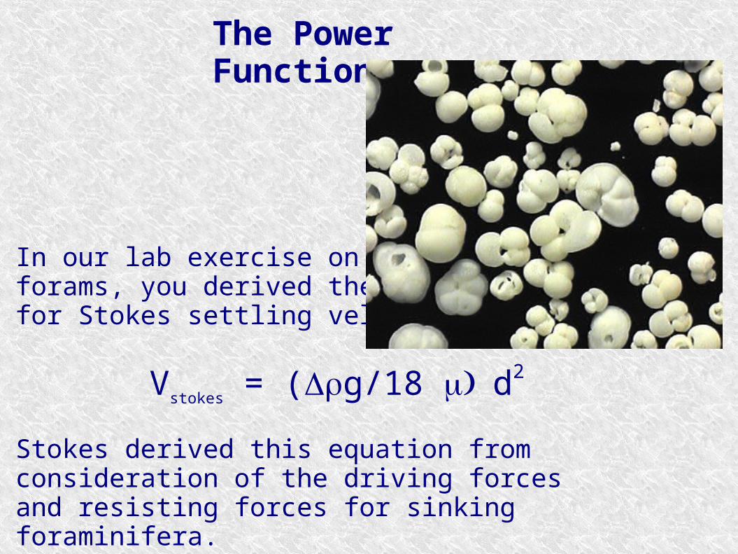
In our lab exercise on sinking forams, you derived the equation for Stokes settling velocity,
Vstokes
= (g/18 d2
Stokes derived this equation from consideration of the driving forces and resisting forces for sinking foraminifera.

The Power Function
Both the empirically defined Hack equation and the analytically derived Law for Stokes velocity are examples of power functions.
A power function is written in general form by
y = axb .

The Power Function
In the case of Hack's Law,
y = Lx = Ab = 0.6(a = 1.4)
L = 1.4 A0.6
y = axb

The Power Function
In the case of Stokes velocity,
y = Vstokes
x = db = 2(a = g/18)
y = axb
Vstokes
= (g/18 d2

The Power Function
y = axb
What is interesting about this equation is what happens when you apply logarithms.
How would you do it ?
log y = log a + b*log x
Does this equation remind you of anything ?

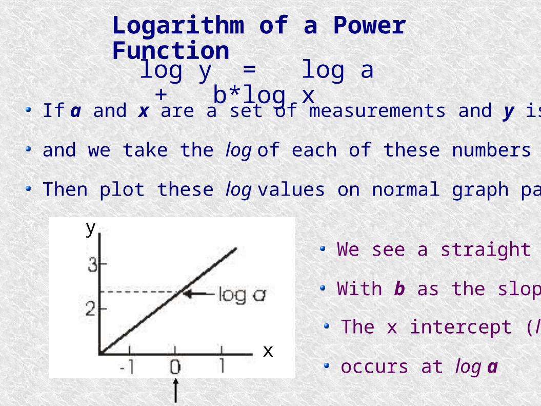
Logarithm of a Power Function
log y = log a + b*log x
This may be similar to the equation for a straight line where y = b + m*x
b = 3m = 1
y = 3 + 1*x y = 3 + x
What kind of scale would we need to plot the logarithmic equation to simulate a linear equation ?
(at the x intercept when x = 0, y = 3)
Logarithm of a Power Function
log y = log a + b*log x
If a and x are a set of measurements and y is a column of results
and we take the log of each of these numbers
Then plot these log values on normal graph paper...
We see a straight line.
With b as the slope.
The x intercept (log x = 0)
occurs at log ax
y

Logarithm of a Power Function
log y = log a + b*log x
If we plot x against y on log-log paper,
We also see a straight line
Again, b is the slope
The line crosses x = 1
Where y = a
x
y

Power Functions in Geology
Log - log plots are common in geology
As a result, power functions often arise in geology
C = CoF(D-1)
As crystals settle out of a magmaelement concentrations, C, in theremaining liquid change accordingto this equation.
Where Co is initial concentration, F is the fraction of liquid remaining, and D is the distribution coefficient.
Linear plot of
C = CoF(D-1)

Power Functions in Geology
Log - log plots are common in geology
As a result, power functions often arise in geology
C = CoF(D-1) log-log plot
log C = log Co + (D-1) log F

Power Functions in Geology
Stream length (y) and drainage-basin area (x) are measuredand listed in the table above.
The logs of each measurement are listed in column 4 and 5
If we plot columns 4 and 5 and try to “fit” a line to the data
Constant = 0.148761, and slope is 0.53687

Power Functions in Geology
Constant = 0.148761, and slope is 0.53687
How can we write this in a linear style equation with logs ?
log y = 0.148761 + 0.53687 log x

Power Functions in Geology
log y = 0.148761 + 0.53687 log x
Plot columns x and y (squares)
Test theory, but plotting the line for the log eqn above.
Pretty good fit!

Power Functions in Geology
log y = 0.148761 + 0.53687 log x
Remember that if we take the “antilog” of both sides
We get y = 100.148761 x0.53687
Simplifying, y = 1.41 x0.54

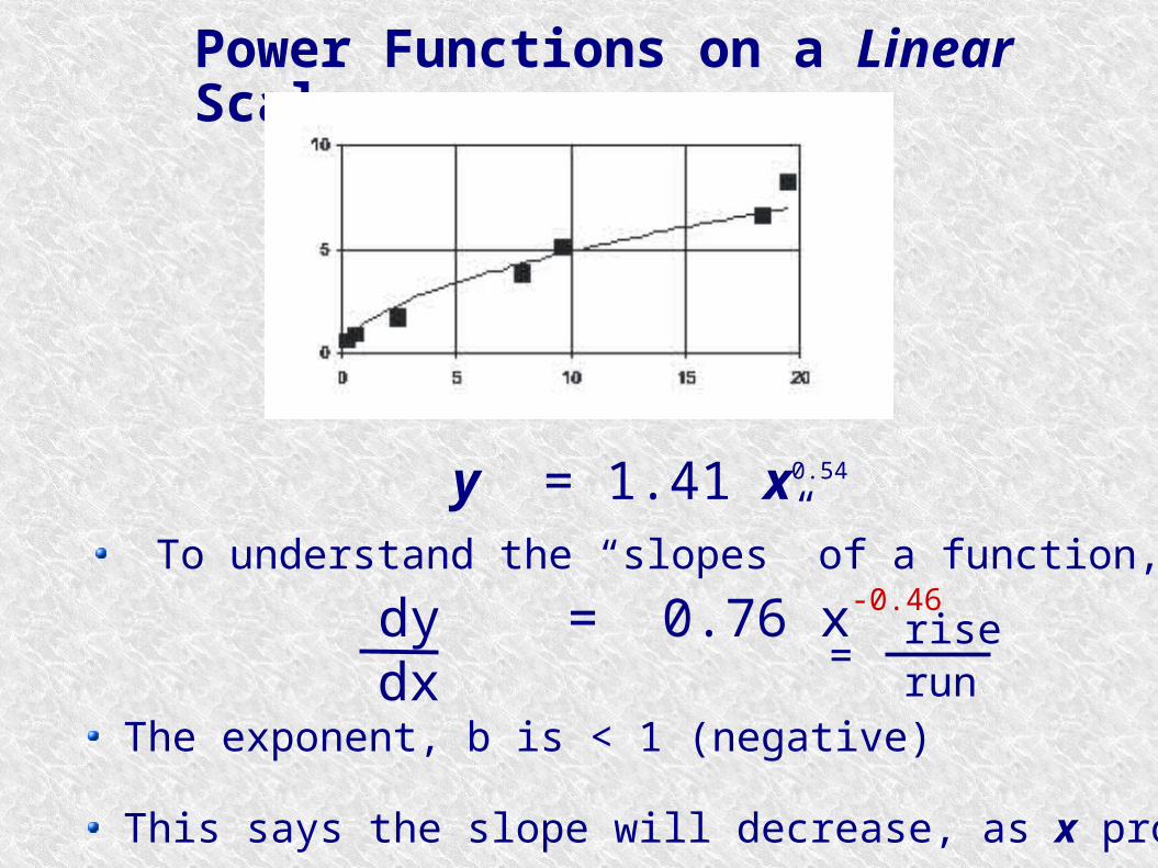
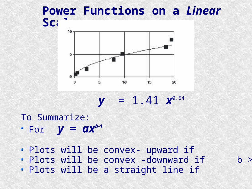
Power Functions on a Linear Scale
y = 1.41 x0.54
Data in a power function plotted on a linear-linear scale
The curve continues to increase
But it increases at an ever decreasing slope
Power Functions on a Linear Scale
y = 1.41 x0.54
To understand the “slopes” of a function, take it's derivative
dy = 0.76 x-0.46
dx The exponent, b is < 1 (negative)
This says the slope will decrease, as x progresses
riserun
=

Power Functions on a Linear Scale
Taking the derivative in general
dy = (a) xb-1
dx If the exponent, b is > 1 (positive)
Then the slope will increase, as x progresses
What if b = 1 ? Then what ?
Power Functions on a Linear Scale
y = 1.41 x0.54
To Summarize: For y = axb-1
Plots will be convex- upward if b < 1 (negative exp) Plots will be convex -downward if b > 1 (positive exp) Plots will be a straight line if b = 1.
Power Functions and Exponential Functions
It is easy to confuse power fns with exponential fns
We've already looked at exponential functions
But we have not studied power functions until today.
y = xb y = bx
Exponential functions produce a straight line when plotted on a linear-log scale.
Where as power functions produce a straight line when plotted on a log-log scale

Power Functions and Exponential Functions
y = xb
In a power function, for every increase in x by some factor y increases by some other factor
In an exponential function, for every increase in x by some factor y may increase by an order of magnitude
(assuming b is a whole number) This is where the concept of a half-life comes from.
y = bx
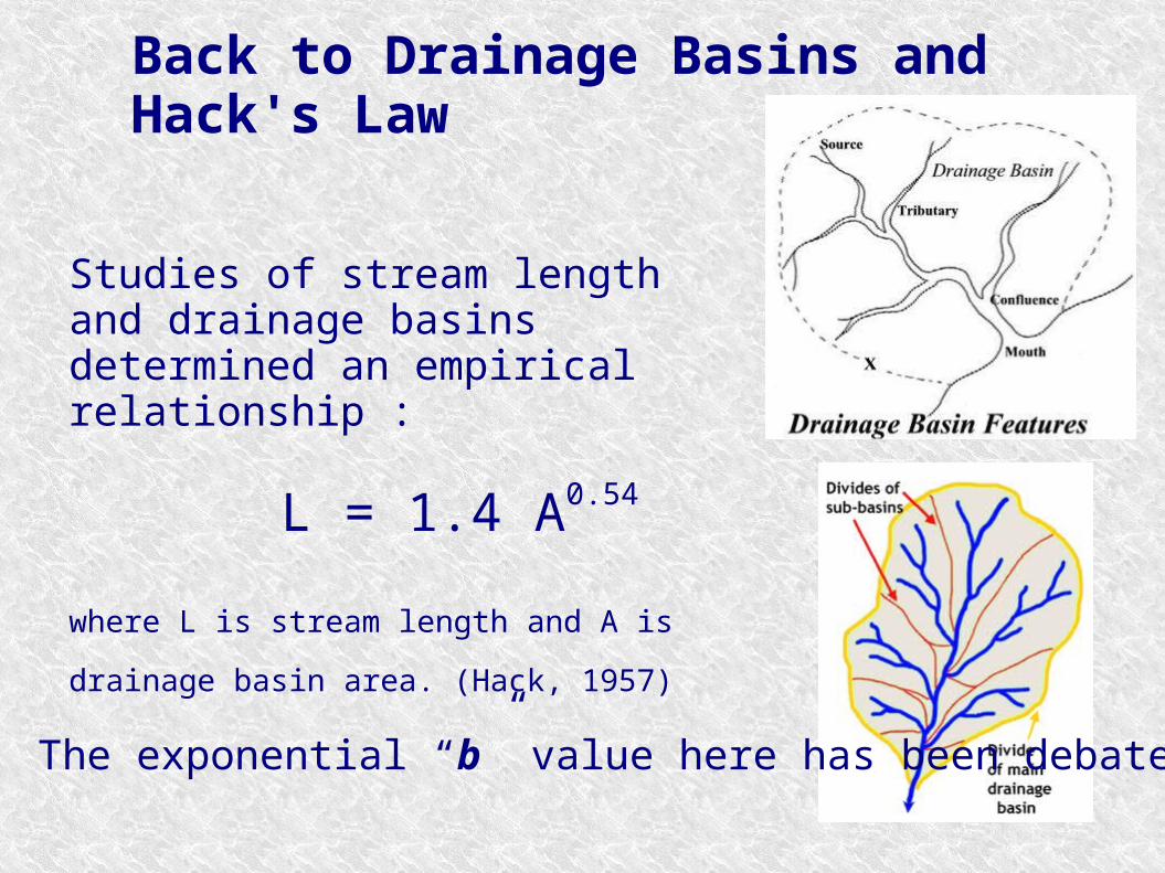
Studies of stream length and drainage basins determined an empirical relationship :
L = 1.4 A0.54
where L is stream length and A is drainage basin
area. (Hack, 1957)
Back to Drainage Basins and Hack's Law
The exponential “b” value here has been debated.

L = 1.4 A0.6
Back to Drainage Basins and Hack's Law
Some say that if b > 0.5
Then the length/area relationship implies that large basins are more elongated.

L = 1.4 A0.54
Shape of Drainage Basins
Understanding length/area ratio
If A = wL
Then, L = 1.4 (wL)0.54
Simplifying.... w/L = 0.53L-0.15
w
L
Notice that the exponent is negative.
How will w/L change as you go downstream (increasing L) ?

Shape of Drainage Basins
Put L on one side: w/L = 0.53L-0.15
w = 0.53 L0.85
Will a plot of L versus w be convex up or down ?
w
L