Embed Size (px)
Citation preview
The Power of Tests for Pareto
Efficiency Within the Family
Jesse Naidoo∗
University of Chicago
JOB MARKET PAPER
This Version: January 19, 2015
Please click here for the latest version of this paper.
JEL codes: D13, D7.
Abstract
Empirical studies of the allocation of consumption within the familyhave often failed to reject the null hypothesis of Pareto efficiency. To studythe power of these tests, I construct two models of public goods allocation.One model is cooperative and leads to efficient allocations, and the otheris noncooperative and leads to inefficient allocations. In the noncoopera-tive models, variations in the economic or social circumstances outside ofthe household (“distribution factors”) cause variations in implicit prop-erty rights within the household. If these variations go unobserved by theeconometrician, then noncooperative models imply the same restrictionson household demand as do the cooperative ones. Therefore, many testsin the literature cannot identify inefficiency when it is present. I thenshow that without restrictions on preferences or data on individual con-sumption, the hypothesis of Pareto efficiency is not well-separated fromthe noncooperative alternative. So in a nonparametric setting, there canbe no tests that both reject all inefficient models and do not reject anyefficient models. However, if the effective wealth of each partner is ob-served without error and satisfies a large support condition, and if theconsumption of a public good and at least one assignable private goodcan be observed, then it is possible to reject efficiency.
∗email: [email protected]. I thank Azeem Shaikh, Alessandra Voena, Robert Gar-lick, Chen Yeh, Elisa Olivieri, Alex Frankel, Stephane Bonhomme, Magne Mogstad, PhilipBarrett and especially Derek Neal for their comments and for their support. All errors aremy own.
1
1 Introduction
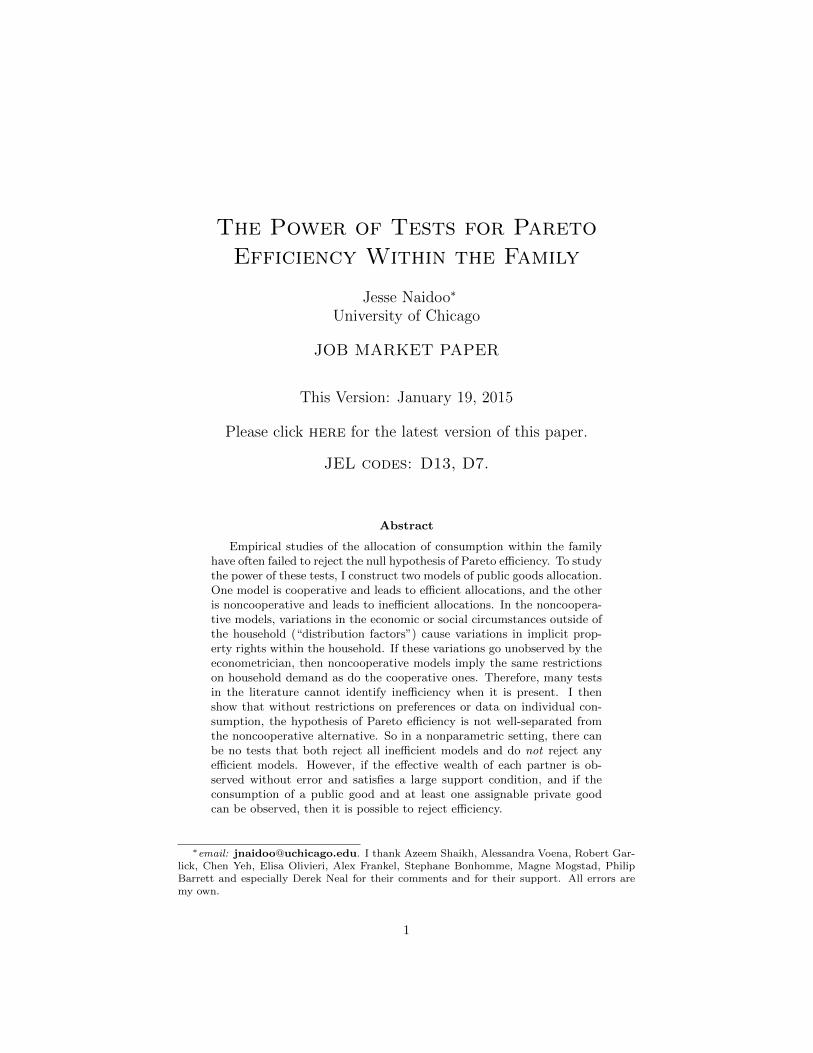
A glance at Table 1 creates the impression that, although the literature is shortof a consensus, Pareto efficiency characterizes family life well. That is, manystudies have failed to reject the null hypothesis of efficiency. What remainsunexamined, though, is whether those tests have power against inefficient al-ternatives - or, to put the question more sharply, whether those tests have theability to identify inefficiency.
Table 1: Selected empirical studies of allocation within the family.A “unitary” model of the family is one in which there exists apositive representative consumer.
Paper Country Subject Conclusions
[Attanasio & Lechene, 2014] Mexico consumer goods favors efficiency[Bayudan, 2006] Philippines time use favors efficiency[Bobonis, 2009] Mexico consumer goods favors efficiency
[Bourguignon et al. , 1993] France consumer goods favors efficiency[Browning et al. , 1994] Canada consumer goods favors efficiency
[Browning & Chiappori, 1998] Canada consumer goods favors efficiency[Chiappori et al. , 2002] US labor supply favors efficiency[Del Boca & Flinn, 2014] US time use favors efficiency[Del Boca & Flinn, 2012] US time use favors efficiency
[Donni, 2007] France consumer goods favors efficiency[Donni & Moreau, 2007] France labor supply favors efficiency
[Duflo, 2003] South Africa child health rejects unitary model[Fortin & Lacroix, 1997] Canada labor supply favors efficiency[Goldstein & Udry, 2008] Ghana land use rejects efficiency[Lise & Yamada, 2014] Japan risk-sharing, credit rejects ex-ante efficiency[Lundberg et al. , 1997] UK consumer goods rejects unitary model
[Mazzocco, 2007] US risk-sharing, credit rejects ex-ante efficiency[Vermeulen, 2005] Netherlands labor supply favors efficiency
[Voena, 2010] US risk-sharing, credit rejects ex-ante efficiency[Udry, 1996] Burkina Faso land use rejects efficiency
To explore the possibility of a false negative, I construct two static models ofthe allocation of goods within a two-person family. If some of the goods arepublic, noncooperative equilibria can be inefficient. But, in Section 4, I showthat both classes of models lead to a certain proportionality condition in thehousehold’s aggregate demand system. Since the failure to reject this conditionhas been widely interpreted as evidence for efficiency, this calculation shows thata popular style of test for efficiency cannot detect inefficiency when it is present.
Next, in Section 5, I turn to the question of whether powerful tests can be con-
2

structed using household-level data. My answer is negative: in Proposition 5,I show that there are demand systems that are consistent with both efficientmodels and inefficient models. Within this class, there are no properties of de-mand that are unique to efficient models. In a nonparametric setting, therefore,there can be no tests that simultaneously do not reject any efficient models anddo reject all inefficient models.
Finally, I use my negative results to reassess the evidence on within-family ef-ficiency and suggest ways to break the identification problem. The suggestionsI will be able to make involve either obtaining richer data on consumption atthe individual, rather than the household level, and obtaining more informationabout the decision mechanisms at work in the household.
I am not claiming that families are always and everywhere inefficient. One canoffer other arguments for efficiency, such as those of [Becker, 1991], based onthe existence of specialization or assortative matching. I am claiming that ananalysis of household-level expenditure patterns cannot be informative.
My results do not rely on the existence of unobserved heterogeneity in prefer-ences. Instead, my argument is that models of efficient allocation have a naturalalternative - namely, that each family member makes voluntary contributions toa public good.1 Absent price variation, the data can only tell us about incomeeffects, not substitution effects, and it is the latter which are needed to assesswhether inefficiency is present, at least at the margin. But since there are mod-els where budget shares do not vary with relative prices, price variation is notalways helpful for identification - unless those cases are ruled out by assumption.So household-level data on demand, by itself, cannot decide the question.
There are at least two reasons to examine the efficiency of the family. First,there is much evidence against the “unitary” model of the family, in which allmembers agree on how to use the household’s resources. That evidence comesfrom many different contexts, but generally consists of the observation thatmerely redistributing resources from one family member to another affects howthose resources are used. If all members had the same preferences, intra-familyredistributions would have no such effects.2 Still, it is possible that efficiencyprevails, but this cannot be taken for granted.
Second, any discussion of the policies of a welfare state must be informed bya view, perhaps implicit, of how of families use and distribute their resources.By definition, welfare states provide transfers to their citizens, and many coun-
1This sort of inefficient model is in no way exotic or pathological, nor is itespecially new: [Chen & Woolley, 2001], [Lundberg & Pollak, 1993], and even earlier[McElroy & Horney, 1981] and [Manser & Brown, 1980] all proposed noncooperative modelsof the family.
2[Thomas, 1990], [Duflo, 2003] and [Lundberg et al. , 1997] are prominent examples of thistype of study, and [Alderman et al. , 1995] is an early summary of the evidence.
3
tries do so both in cash and in kind; public education and healthcare are onlythe most expensive examples of in-kind transfers. As [Becker & Murphy, 1988]point out, both sorts of transfers can be motivated by a concern for the well-being of the next generation. But for a policymaker with those concerns, thetwo tools may be substitutes. It can only make sense to examine their usefulnesstogether, and doing so entails taking a stand on intrafamily efficiency.
Other economists before me have raised questions about the strength of the evi-dence for “collective” models of the family. The closest relatives of my work are[Del Boca & Flinn, 2012] and [Del Boca & Flinn, 2014]. In the first of those twopapers, the authors use time-use data from the 2005 wave of the Panel Study ofIncome Dynamics (PSID) to estimate both a cooperative and a non-cooperativemodel of labor supply and housework. They find that over three-quarters of thecouples in their sample manage to achieve efficiency, at least in a static sense.
However, their econometric models differ substantially from mine. Theirs is amixture model, so they attribute unexplained differences in time allocation tounobserved differences across households in preferences, home production tech-nologies, and participation constraints. By contrast, most of the papers in theintrahousehold allocation literature, such as those in Table 1, avoid implying adegenerate distribution of the data by invoking measurement error in consump-tion. To be consistent with this literature, that is also the approach I take here.
[Del Boca & Flinn, 2014] uses the same economic model as [Del Boca & Flinn, 2012],but links it to a Gale-Shapley matching algorithm. They do so in order to incor-porate marriage market patterns into their examination of the efficiency of timeallocation for a sample of American couples from the 2007 wave of the PSID.They conclude that their sample is best characterized by Pareto efficiency withinmarriage, but do not formally test that claim. ([Del Boca & Flinn, 2012] alsodo not define or test Pareto efficiency econometrically.) Instead, they show thatthe distribution of a likelihood ratio statistic is such that efficiency is a bettercharacterization of their sample. In this paper, I take a more formal approachto the identification of inefficiency.
[Cherchye et al. , 2007] and [Cherchye et al. , 2009] are methodologically moredistant from this paper, although again the questions they address are similar tomine. They provide revealed-preference conditions on household consumptionwhich, they argue, are necessary and sufficient for Pareto optimality. Again,unlike much of the literature in Table 1, those conditions treat a household’sobserved purchases as exact data, free of measurement error.
In Section 2 below I begin my analysis, by stating my assumptions about theinformation available to an imagined econometrician.
4
2 Econometric Preliminaries
2.1 Consumption Data
I assume the econometrician has access to a dataset consisting of observationsof many households. These households themselves consist of two members each;I will refer to the two members as A and B. Later, it will become importantthat prices do not vary across households, so it may be easiest to imagine thatthe data is cross-sectional.
Let P be a vector of prices, of dimension m + 1, for some integer m ≥ 1. LetQ be a vector of quantities purchased by a given household, so the dimensionof Q is also m + 1. I think of Q as the vector of a given household’s aggregateconsumption. It is often difficult to attribute the expenditures on consumergoods, such as food, to either A or B, and furthermore, some consumption maygenuinely be “public,” such as expenditures on children. So for now I will as-sume that the econometrician cannot disaggregate the vector Q into separateaccounts for public consumption and for the private consumption of A and Beach.
Together, A and B have wealth Y at their disposal; and finally, let Z be a vectorof social or economic variables which I will call “distribution factors”. These arevariables which may affect the consumption of a household, but not its budgetset. For example, some authors have used the local sex ratio - understood asa proxy for conditions on the marriage market - as a distribution factor. Itis certainly true that variables can sometimes be found that do not directlyaffect the income of, or prices facing, any given household, but are correlatedwith consumption patterns nonetheless. However, the economic mechanism bywhich the variables in Z affect the household’s choice of Q is, for now, left un-stated. Most of what I will have to say concerns how to interpret the empiricalrelationship between Z and Q.
2.2 Household Demand Systems
I assume that the econometrician has enough data so that the joint distributionof (P,Q, Y, Z) is known with certainty, and therefore so is the conditional meanin the population
g(p, y, z) = E[Q|P = p, Y = y, Z = z]. (1)
In making this assumption, I am avoiding the complications of inference in finitesamples, and focusing only on the logical possibilities for the identification ofinefficiency under various assumptions about the domain of (p, y, z) over whichg can be observed.
5
Let U ⊂ Rm+1++ × R++ and V ⊂ RK be open. U is the domain for prices and
household wealth, (p, y); V is the domain for the distribution factors z.
Definition 1. Let g : U ×V −→ Rm+1++ be continuously differentiable and such
that, for all (p, y, z) ∈ U × V ,
m∑i=0
pigi(p, y, z) = y. (2)
Then g is called an extended aggregate demand system on U × V . 4
Given a pair of open sets (U, V ) of appropriate dimensions, let G(U, V ) denotethe set of all extended aggregate demand systems on the domain U × V .
In most cross-sectional data, though, all households face the same prices. So itwill be important to allow for the possibility that, for some p, only the condi-tional distribution of (Q,Y, Z) given P = p, can be known by the econometri-cian.
To that end, let p be such that for some y > 0, (p, y) ∈ U and define thep-section of U × V as
(U × V )|p = {(y, z) : (p, y) ∈ U, z ∈ V }. (3)
By multiplying each quantity gi(p, y, z) by its price pi, one puts the quantitiesrepresented by g(p, y, z) into expenditure form; let hi(y, z|p) = pi · gi(p, y, z)represent total expenditure on the ith good. The above domain restriction andchange of units leads to the following definition:
Definition 2. Let p be such that for some y > 0, (p, y) ∈ U . A restrictedaggregate demand system on (U × V )|p is a continuously differentiable function
h : (U × V )|p −→ Rm+1++ such that for all (y, z)
m∑i=0
hi(y, z) = y. (4)
4
I write H(U, V |p) for the set of all such functions. At any suitable p, each ex-tended aggregate demand system g ∈ G(U, V ) induces a restricted aggregatedemand system h ∈ H(U, V |p), in the way indicated by equation (2).
I also assume that only “nondegenerate” demand systems are of interest, in thefollowing sense:
6
Definition 3. Let h ∈ H(U, V |p) be a restricted aggregate demand system,and define
hi = sup
{hi(y, z)
y: (y, z) ∈ (U × V )|p
}(5)
hi = inf
{hi(y, z)
y: (y, z) ∈ (U × V )|p
}(6)
If h is such that, for all goods 0 ≤ i ≤ m,
0 < hi < hi < 1 (7)
then say that h is nondegenerate. 4
h is degenerate if the budget share of at least one good either (i) does not varyat all in the data (so hi = hi), (ii) has vanishing consumption (so hi = 0),or (iii) occupies the households’ entire budget (hi = 1). If h is interpreted asa population average, the common microeconometric problems associated withinfrequent purchases do not arise. Thus, imposing that h be nondegenerateseems like a weak requirement.
3 Two Models of Allocation Within the Family
Below, I construct two parallel formulations of an intrahousehold allocationproblem. One model leads to efficient allocations, which, following [Chiappori, 1992],I call a “collective” model of the household. The second model leads to ineffi-cient allocations.
I call the second family of models I construct “Cournot” models, because oftheir resemblance to that classical model of imperfect competition. Inefficiencyexists in equilibrium because both A and B contribute voluntarily and nonco-operatively to a public good. Thus, under a Cournot model, the equilibriumconsumption of the public good is too low. I need to assume the existence ofa public good, otherwise the first welfare theorem implies that noncooperativedecision-making is efficient. (Of course, if all goods are private, there are nogains from marriage either.)
3.1 Cournot and Collective Models: Definition
3.1.1 Collective Models
A model of the efficient allocation of goods in a many-person family has twocomponents: (i) a description of the family members’ individual preferencesover the goods, including a list of which goods are public and which are pri-vate, and (ii) a description of which particular efficient allocation will be chosen,and how that “collective” choice varies with the parameters describing the fam-ily’s environment. In the context of Section 2 above, the family’s environment
7
is characterized by its budget set and the distribution factors, i.e. the tuple(p, y, z). Formalizing this, we have the following:
Definition 4. Let I ⊂ {0, 1, . . .m} and write n = |I|. By permuting indices,we may assume I = {0, 1, . . . n − 1}. Write qAB for the first n components ofthe vector of aggregate purchases.
Also let uA, uB be weakly increasing and quasiconcave functions on Rm+1++ , and
say µ : U × V −→ (0, 1) is smooth. Given (p, y, z), consider the social planner’sproblem
max(qAB ,qA,qB)
µ · uA(qAB , qA) + [1− µ] · uB(qAB , qB)
subject ton−1∑i=0
piqAB,i +
m∑i=n
pi(qA,i + qB,i) ≤ y. (8)
If (8) has a unique solution (q∗∗AB , q∗∗A , q
∗∗B ) ∈ Rn++ × Rm+1−n
++ × Rm+1−n++ for all
(p, y, µ) ∈ U × (0, 1), and the function
g∗∗(p, y, µ(p, y, z)) = (q∗∗AB , q∗∗A + q∗∗B ) (9)
is continuously differentiable on U × V , then the tuple (I, uA, uB , µ) is called acollective model with n public goods. 4
Given open sets U ⊂ Rm+1++ × R++ and V ⊂ RK , write Θn(U, V ) for the set of
all collective models with n public goods defined for the domain (U, V ), and let
Θ(U, V ) =
m+1⋃n=0
Θn(U, V ) (10)
be the set of all collective models on (U, V ). I will use θ = (I, uA, uB , µ) todenote a typical collective model in Θ(U, V ).
The function µ is often called the “Pareto weight”, and inspection of (8) showsthat higher values of µ “tilt” the household’s decisions towards A’s preferences:the optimal value of uA is increasing in µ, and the optimal value of uB isdecreasing in µ. µ is allowed to depend on the economic and social environmentof the household, (p, y, z).
Example 1. Suppose m = 2, so there are three goods in total: a public goodq0 and two private goods q1, q2. Assume that goods 1 and 2 are “exclusive”, sothat A does not consume good 2 and B does not consume good 1. Preferencesare
uA(q0, qA1) = α log(q0) + (1− α) log(qA1) (11)
uB(q0, qB1) = β log(q0) + (1− β) log(qB2) (12)
8
for some 0 < α, β < 1. Normalizing the price of the public good to unity, letp = (1, p1, p2) be the price vector, and let household wealth y be given.
For any µ ∈ [0, 1], the efficient allocation is
q0 = y · [µα+ (1− µ)β] (13)
qA1 =y
p1· µ(1− α) (14)
qA2 = 0 (15)
qB1 = 0 (16)
qB2 =y
p2· (1− µ)(1− β). (17)
To complete the description of this collective model, suppose A and B supplylabor inelastically, earning wages zA and zB , and suppose that the Pareto weightµ is given by
µ(y, zA, zB) =1
2y(y + zA − zB). (18)
A’s Pareto weight, µ, depends positively on zA and negatively on zB , perhapsbecause each individual’s wages are correlated with their outside option on themarriage market.
The aggregate demands generated by this collective model are
g∗∗0 (p, y, µ(y, zA, zB)) = y · [αµ(y, zA, zB) + β(1− µ(y, zA, zB))]
= α · 1
2(y + zA − zB) + β · 1
2(y + zB − zA) (19)
g∗∗1 (p, y, µ(y, zA, zB)) =y
p1· (1− α)µ(y, zA, zB)
=(1− α)
2p1· (y + zA − zB) (20)
g∗∗2 (p, y, µ(y, zA, zB)) =y
p2· (1− β)(1− µ(y, zA, zB))
=(1− β)
2p2· (y + zA − zB) (21)
4
3.1.2 Cournot Models
Under a collective model, variations in the distribution factors z at fixed valuesof (p, y) cause the household to move along a utility possibility frontier. Those
9
variations along a fixed Pareto frontier cause changes in the aggregate consump-tion patterns of the household.
However, changes in a family’s consumption can be caused by variations in theintrahousehold distribution of resources, too. An empirical relationship betweendistribution factors z and consumption can also be rationalized by models whichallow for distribution factors and (perhaps implicit) property rights within thefamily to be correlated.
Example 2. As before, suppose A and B supply labor inelastically, earningwages zA and zB . They also have nonlabor wealth zAB , to which they haveequal claim. Thus,
y = zA + zB + zAB . (22)
Since each member of the household has equal claim to the “joint” wealth zAB ,and full claim to his or her own labor earnings, A’s total wealth is
yA = zA +1
2zAB
=1
2(y + zA − zB) (23)
and A’s effective share of household wealth is
ω(y, zA, zB) =1
2y(y + zA − zB). (24)
4
A noncooperative model of allocation in a many-person family has similar in-gredients to a collective one, namely (i) a description of the preferences of thefamily members, and (ii) a description of how control over the family’s resourcesvaries with the social and economic environment. I formalize this below.
Definition 5. Let I ⊂ {0, 1, . . .m} be a singleton. By permuting indices, wemay assume I = {0}.
Also let uA, uB be weakly increasing and quasiconcave functions on Rm+1++ , and
say ω : U × V −→ (0, 1) is smooth. Consider the system
max(qA0,qA)
uA(qA0 + qB0, qA) s.t. p0qA0 +
m∑i=1
piqAi ≤ yω (25)
max(qB0,qB)
uB(qA0 + qB0, qB) s.t p0qB0 +
m∑i=1
piqBi ≤ y(1− ω). (26)
10

If the system (25) - (26) has a unique solution ((q∗A0, q∗A), (q∗B0, q
∗B)) for all
(p, y, ω) ∈ U × (0, 1), and the function
g∗(p, y, ω(p, y, z)) = (q∗A0 + q∗B0, q∗A + q∗B) (27)
is continuously differentiable in (p, y, ω) on U ×V , then the tuple (I, uA, uB , ω)is called a Cournot model with one public good. 4
The system (25) - (26) defines the Nash equilibrium of a simultaneous-movegame in which A and B make voluntary contributions to a public good. Theirstrategies (and actions) are their contributions qA0 and qB0. Their strategyspaces are [0, yω/p0] for A and [0, y(1− ω)/p0] for B.3
3.2 Scope and Interpretation of the Models
Both collective and Cournot models concern allocation within an existing fam-ily. The functions µ and ω are mechanisms that select an allocation, given thepreferences of A and B, but their interpretations are different. Neither classof model places any structure on the relationship between the decision processwithin the family and its external circumstances, as represented by the variables(p, y, z).
A natural way to think of the Pareto weight µ is that it represents the oppor-tunity cost of marriage, while the function ω represents the share of householdresources controlled by A - her “property rights” within the household. Ofcourse, ω may be determined in part by explicit laws about the division ofproperty (as in Example 2 above), but the effective control each member of thefamily can exert is likely to be affected by other factors, such as local culturalnorms and understandings of gender roles.
3.3 Properties of Cournot Models
3.3.1 Existence and Uniqueness of Equilibrium
Let Γ(U, V ) denote the set of all Cournot models defined over (U, V ), and writeγ = (I, uA, uB , ω) for a single Cournot model. Definition 5 requires that theequilibrium defined by the best-response functions (25) - (26) is unique, but itis not immediate that there are preferences uA and uB such that it will be.
The following example exhibits preferences uA and uB such that the equilib-rium exists and is unique for all (p, y, ω) ∈ U × (0, 1); furthermore, the equilib-rium allocations g∗(p, y, ω) depend smoothly on (p, y, ω), except at two points
3It is important to assume that there is only one public good, because that assumption,along with a mild normality condition on the preferences of A and B, will be sufficient toguarantee that the equilibrium allocation is unique. I discuss those conditions further inSection 3.3.1.
11
ω∗, ω∗ ∈ (0, 1).
Thus, if the map ω is such that neither ω∗ nor ω∗ are in its range ω(U × V ),then we will have found a Cournot model γ meeting Definition 5, and hence wecan conclude that the set Γ(U, V ) is nonempty.
Example 3. As in Example 1, let there be three goods in total: a public goodq0 and two private goods q1, q2. Again assume preferences are
uA(q0, qA1) = a log(q0) + (1− a) log(qA1) (28)
uB(q0, qB1) = b log(q0) + (1− b) log(qB2) (29)
for some 0 < a, b < 1. Let yA, yB be the wealth levels of the two family members.
If we normalize the p0, the price of the public good, to unity, A’s decisionproblem is
maxqA0,qA1
a log(qA0 + qB0) + (1− a) log(qA1) s.t qA0 + p1qA1 ≤ yA (30)
given B’s contribution qB0. But since the total consumption of the public goodis q0 = qA0 + qB0, we can rewrite A’s problem as
maxq0,qA1
a log(q0) + (1− a) log(qA1) s.t q0 + p1qA1 ≤ yω + qB0 (31)
q0 ≥ qB0 (32)
which has the solution
q∗A0(p, yA, qB0) =
{a(yA + qB0)− qB0 if qB0 < a(yA + qB0)0 if qB0 ≥ a(yA + qB0)
(33)
p1 · q∗A1(p, yA, qB0) =
{(1− a)(yA + qB0) if qB0 < a(yA + qB0)yA if qB0 ≥ a(yA + qB0)
(34)
Similarly, B’s best response is
q∗B0(p, yB , qA0) =
{b(yB + qA0)− qA0 if qA0 < b(yB + qA0)0 if qA0 ≥ b(yB + qA0)
(35)
p2 · q∗B2(p, yB , qA0) =
{(1− b)(yB + qA0) if qA0 < b(yB + qA0)yB if qA0 ≥ b(yB + qA0)
(36)
An equilibrium for this “Cournot” game is a pair (q∗A0, q∗B0) ∈ [0, yω/p0] ×
[0, y(1 − ω)/p0] such that solves (33) and (35) simultaneously; the equilibriumlevels of private consumption q∗A1 and q∗B2 are then implicitly determined by Aand B’s individual budget constraints.
Let ω = yA/(yA + yB) be A’s (legally defined) share of the household’s totalwealth, y = yA + yB . The unique equilibrium of this public-goods game is
12
q∗A0 =
0 if ω < ω∗y · [aω − (1− a)b(1− ω)] if ω ∈ (ω∗, ω
∗)aω · y if ω ≥ ω∗
(37)
q∗B0 =
y · b(1− ω) if ω < ω∗y · [b(1− ω)− (1− b)aω] if ω ∈ (ω∗, ω
∗)0 if ω ≥ ω∗
(38)
where ω∗ and ω∗ solve
aω∗ − (1− a)b(1− ω∗) = 0 (39)
bω∗ − (1− b)aω∗ = 0 (40)
i.e.
ω∗ =b(1− a)
1− (1− a)(1− b)(41)
ω∗ =b
1− (1− a)(1− b)(42)
Hence, aggregate demands are
g∗0(p, y, ω) =
y · b(1− ω) if ω < ω∗
y · ab1−(1−a)(1−b) if ω ∈ (ω∗, ω
∗)
y · aω if ω ≥ ω∗
(43)
g∗1(p, y, ω) =
yp1· ω if ω < ω∗
yp1· (1−a)b1−(1−a)(1−b) if ω ∈ (ω∗, ω
∗)
yp1· (1− a)ω if ω ≥ ω∗
(44)
g∗2(p, y, ω) =
yp2· (1− b)(1− ω) if ω < ω∗
yp2· b1−(1−a)(1−b) if ω ∈ (ω∗, ω
∗)
yp2· (1− ω) if ω ≥ ω∗
(45)
Figure 1 depicts the aggregate demands g∗(p, y, ω) as a function of A’s relativewealth, ω. Now, if the range ω(U × V ) is contained in either (0, ω∗) or (ω∗, 1),then the tuple γ = ({0}, uA, uB , ω) is a Cournot model in the sense of Definition5; that is, γ ∈ Γ(U, V ). 4
13
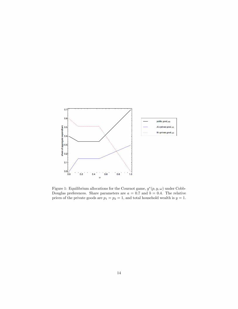
Figure 1: Equilibrium allocations for the Cournot game, g∗(p, y, ω) under Cobb-Douglas preferences. Share parameters are a = 0.7 and b = 0.4. The relativeprices of the private goods are p1 = p2 = 1, and total household wealth is y = 1.
14
Example 3 contains two lessons. First, the conditions under which a unique equi-librium of the public goods game exists are fairly mild. In the above example,a unique equilibrium exists whenever the best-response functions (33) and (35)have a unique intersection (q∗A0, q
∗B0), and this was always the case because both
a and b lay in the interval (0, 1). The fact that preferences were Cobb-Douglasis not essential: as long as the slope of each partners’ Engel curve for the publicgood is strictly between zero and one, there will be a unique equilibrium. Inother words, we have the following:
Proposition 1. Let qA0(p, yA) be A’s Marshallian demand for the public good,and similarly for qB0(p, yB). If, for all (p, yA, yB), 0 < ∂qA0(p, yA)/∂yA < 1,and 0 < ∂qB0(p, yB)/∂yB < 1, then the public goods game of Definition 5 has aunique Nash equilibrium.
Proof. This is simply a restatement of Theorems 2 and 3 of [Bergstrom et al. , 1986]).
Second, by inspection of (43) - (45), one can see that variations in prices p andhousehold wealth y do not change the qualitative properties of the aggregatedemands: when A is “sufficiently poor” relative to B, A will not contribute tothe public good; when B is sufficiently poor relative to A, the reverse happens;and when A and B are nearly equally endowed, both will contribute to thepublic good.4 Formalizing this, we have:
Proposition 2. Let qA0(p, yA) be A’s Marshallian demand for the public good,and similarly let qB0(p, yB) be B’s Marshallian demand for the public good.Normalize the price of the public good p0 to unity, and fix the other prices(p1 . . . pm) and the aggregate endowment y. Let A’s effective share be ω, andwrite q∗A(ω|p, y) and q∗B(1 − ω|p, y) for the equilibrium quantities of A and B’sprivate consumption.
Then there exist scalars ω∗(p, y), ω∗(p, y), with 0 < ω∗ < ω∗ < 1, such that theshares of aggregate consumption devoted to each partner’s private consumptionare:
4It can be shown that when both partners contribute to the public good, its aggregateconsumption is invariant to small redistributions of the endowment. (That result is stated inTheorem 1 of [Bergstrom et al. , 1986].) But, given the budget constraints of each partner,the value of the private consumption of each partner must be locally constant in ω too,although the composition of their private consumption may change. This is visually obviousin Figure 1, since all budget shares pig
∗i (p, y, ω)/y are flat whenever ω ∈ (ω∗, ω∗). However,
this “income-pooling” zone will not be useful for my analysis, so I leave it aside.
15
y−1m∑i=1
piq∗Ai(ω|p, y) =
ω if ω ∈ [0, ω∗]
ω∗ if ω ∈ (ω∗, ω∗)
ω − y−1qA0(p, yω) if ω ∈ [ω∗, 1]
(46)
y−1m∑i=1
piq∗Bi(ω|p, y) =
(1− ω)− y−1qB0(p, (1− ω)y) if ω ∈ [0, ω∗]
1− ω∗ if ω ∈ (ω∗, ω∗)
(1− ω) if ω ∈ [ω∗, 1]
(47)
Proof. See Appendix A.
3.3.2 Inefficiency of Equilibrium
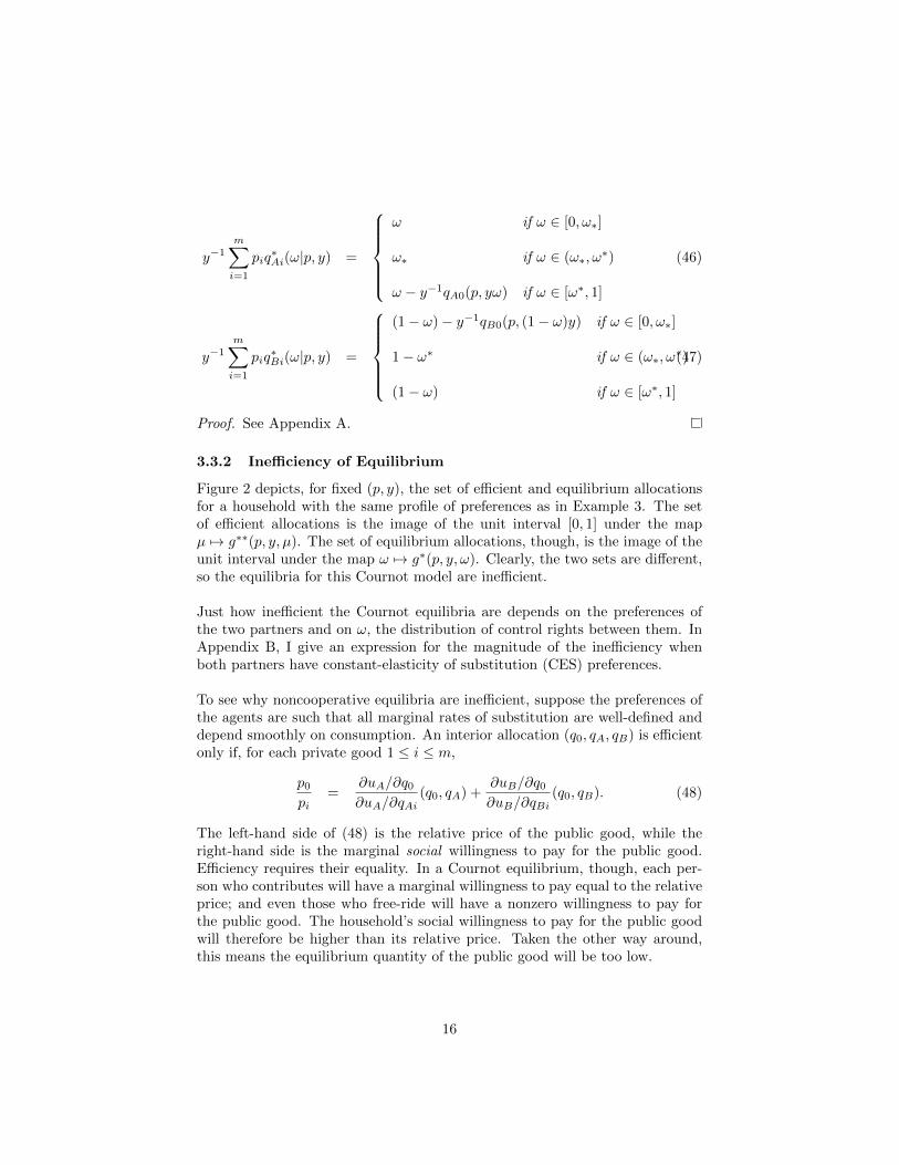
Figure 2 depicts, for fixed (p, y), the set of efficient and equilibrium allocationsfor a household with the same profile of preferences as in Example 3. The setof efficient allocations is the image of the unit interval [0, 1] under the mapµ 7→ g∗∗(p, y, µ). The set of equilibrium allocations, though, is the image of theunit interval under the map ω 7→ g∗(p, y, ω). Clearly, the two sets are different,so the equilibria for this Cournot model are inefficient.
Just how inefficient the Cournot equilibria are depends on the preferences ofthe two partners and on ω, the distribution of control rights between them. InAppendix B, I give an expression for the magnitude of the inefficiency whenboth partners have constant-elasticity of substitution (CES) preferences.
To see why noncooperative equilibria are inefficient, suppose the preferences ofthe agents are such that all marginal rates of substitution are well-defined anddepend smoothly on consumption. An interior allocation (q0, qA, qB) is efficientonly if, for each private good 1 ≤ i ≤ m,
p0pi
=∂uA/∂q0∂uA/∂qAi
(q0, qA) +∂uB/∂q0∂uB/∂qBi
(q0, qB). (48)
The left-hand side of (48) is the relative price of the public good, while theright-hand side is the marginal social willingness to pay for the public good.Efficiency requires their equality. In a Cournot equilibrium, though, each per-son who contributes will have a marginal willingness to pay equal to the relativeprice; and even those who free-ride will have a nonzero willingness to pay forthe public good. The household’s social willingness to pay for the public goodwill therefore be higher than its relative price. Taken the other way around,this means the equilibrium quantity of the public good will be too low.
16
Figure 2: Equilibrium and efficient allocations under Cobb-Douglas preferences.Share parameters are a = 0.7 and b = 0.4. The relative prices of the privategoods are p1 = p2 = 1, and total household wealth is y = 1. The black line isthe set of Cournot equilibrium allocations, g∗(p, y, ω). The dashed blue line isthe set of efficient allocations, g∗∗(p, y, µ).
Having constructed both an efficient and an inefficient model, we are finally ina position to see whether the sort of consumption data described in Section 2above can distinguish between them.
4 Tests of Distribution Factor Proportionality
By definition, both collective and Cournot models induce extended demandsystems on U × V . In view of that fact, I will abuse notation slightly and writeg∗∗(p, y, z|θ) ∈ G(U, V ) and g∗(p, y, z|γ) ∈ G(U, V ). Similarly, at any suitablep, define h∗∗(y, z|θ) ∈ H(U, V |p) to be the restricted aggregate demand systemimplied by the collective model θ at p:
h∗∗(y, z|θ) =
p0g∗∗0 (p, y, z|θ)
p1g∗∗1 (p, y, z|θ)
...pmg
∗∗m (p, y, z|θ)
(49)
17
The obvious analogue for Cournot models is
h∗(y, z|γ) =
p0g∗0(p, y, z|γ)
p1g∗1(p, y, z|γ)
...pmg
∗m(p, y, z|γ)
. (50)
The problem facing the econometrician is to determine whether a given h ∈H(U, V |p) was generated by a collective model, by a Cournot model, or neither.That is, is h = h∗∗(·|θ) for some θ ∈ Θ(U, V )? Alternatively, is h = h∗(·|γ) forsome γ ∈ Γ(U, V )? An obvious place to start would be finding conditions on himplied by efficiency. In fact, there are such conditions, as first introduced by[Browning & Chiappori, 1998].
Definition 6. Let h ∈ H(U, V |p) be a restricted aggregate demand system suchthat no distribution factor is redundant, i.e. for all goods i and all distributionfactors zk,
∂hi∂zk
(y, z) 6= 0 (51)
for all (y, z) ∈ (U × V )|p. If, for all (y, z) ∈ (U × V )|p, and all goods i, i′ andall distribution factors k, k′,
∂hi/∂zk∂hi/∂zk′
=∂hi′/∂zk∂hi′/∂zk′
(52)
then say that h satisfies distribution factor proportionality (DFP) on (U × V )|p.4
For a strictly concave representation of preferences, efficiency is equivalent tothe existence of a Pareto weight µ. And because the distribution factors only acton demands through their effects on a scalar index - namely µ - the chain ruleimplies that the effects of different distribution factors must be proportional.For if h is induced by a collective model, we can write
h(y, z) = h∗∗(y, µ(y, z)|θ) (53)
Differentiating, we obtain that for any good i, and any two distribution factorsk, k′,
∂hi∂zk
=∂h∗∗i∂µ· ∂µ∂zk
(54)
∂hi∂zk′
=∂h∗∗i∂µ· ∂µ∂zk′
(55)
Because no distribution factor is redundant, we can divide (54) by (55), so forall goods i,
18
∂hi/∂zk∂hi/∂zk′
=∂µ/∂zk∂µ/∂zk′
. (56)
In short, we have the following:
Proposition 3. If the restricted aggregate demand system h ∈ H(U, V |p) isinduced by a collective model, h satisfies distribution factor proportionality.
Proposition 3 appears to give a way of testing efficiency, even with quite limiteddata. In fact, [Bourguignon et al. , 2009] endorse the testing of distribution fac-tor proportionality as the sole implication of efficiency in data without variationin relative prices.5
However, distribution factor proportionality is also a property of Cournot mod-els. Just like collective models, Cournot models imply that the distributionfactors only act on demands through a scalar index, namely ω. So for the samereasons that collective models imply distribution factor proportionality, Cournotmodels do too.
Proposition 4. If the restricted aggregate demand system h ∈ H(U, V |p) isinduced by a Cournot model, h satisfies distribution factor proportionality.
Proof. Let h be induced by a Cournot model. We can write
h(y, z) = h∗(y, ω(y, z)|γ) (57)
Differentiating and taking ratios as in the proof of Proposition 3, we have theresult.
Proposition 4 means that a test of distribution factor proportionality cannot beinterpreted as a test of Pareto efficiency, because it will have no power againstCournot alternatives. Much of the evidence in Table 2 is therefore not persua-sive.
5When the data do contain variation in relative prices, efficiency also implies a sepa-rate set of properties on the price and wealth derivatives of the extended demand systemg∗∗(p, y, µ(p, y, z)). For completeness, I state these conditions in Appendix C.
19

Tab
le2:
Stu
die
sF
ail
ing
toR
ejec
tE
ffici
ency
inH
ou
seh
old
Con
-su
mp
tion
.E
ach
au
thor
esti
mate
sei
ther
an
exte
nd
edor
rest
rict
edaggre
gate
dem
an
dsy
stem
an
dte
sts
the
imp
lied
rest
rict
ion
sli
sted
un
der
“P
rop
erti
esT
este
d”.
Iab
bre
via
te“d
istr
ibu
tion
fact
or
pro
-p
ort
ion
ali
ty”
to“D
FP
”.
“S
R1”
isa
pro
per
tyth
at
can
on
lyb
ete
sted
ind
ata
wit
hre
lati
vep
rice
vari
ati
on
,an
dis
der
ived
inA
p-
pen
dix
C.
Pap
er
Cou
ntr
yG
ood
sD
istr
ibu
tion
Facto
rsU
sed
Pro
pert
ies
Test
ed
[Att
anas
io&
Lec
hen
e,20
14]
Mex
ico
starc
hes
rela
tive
non
lab
or
inco
me
DF
Pp
uls
esre
lati
vesi
zean
dw
ealt
hof
exte
nd
edfa
mil
yfr
uit
an
dveg
etab
les
mea
t,fi
sh,
an
dd
air
yoth
erfo
od
s[B
ayu
dan
,20
06]
Ph
ilip
pin
esti
me
use
(wiv
eson
ly)
rela
tive
wages
DF
Pse
lf-r
eport
edin
flu
ence
[Bob
onis
,20
09]
Mex
ico
chil
dcl
oth
ing
rela
tive
non
lab
or
inco
me
DF
Pm
en’s
an
dw
om
en’s
cloth
ing
rain
fall
sch
ooli
ng
food
cate
gori
es[B
ourg
uig
non
etal.
,19
93]
Fra
nce
men
’san
dw
om
en’s
cloth
ing
rela
tive
non
lab
or
inco
me
DF
Pfo
od
at
hom
efo
od
at
rest
au
rants
hea
lth
care
cosm
etic
sb
ooks
an
dm
usi
c“va
cati
on
”en
tert
ain
men
t
20

[Bro
wn
ing
etal.
,19
94]
Can
ad
am
en’s
an
dw
om
en’s
cloth
ing
rela
tive
age
DF
Pre
lati
vela
bor
inco
me
[Bro
wn
ing
&C
hia
pp
ori,
1998
]C
an
ad
am
en’s
an
dw
om
en’s
cloth
ing
rela
tive
age
SR
1;
food
at
hom
ere
lati
vela
bor
inco
me
DF
Pfo
od
at
rest
au
rants
tran
sport
ati
on
“se
rvic
es”
alc
oh
ol
an
dto
bacc
o[C
hia
pp
ori
etal.
,20
02]
US
lab
or
sup
ply
loca
lse
xra
tio
DF
Plo
cal
div
orc
ela
ws
[Don
ni,
2007
]F
ran
cela
bor
sup
ply
(wif
eon
ly)
rela
tive
wages
DF
Pfo
od
(aggre
gate
d)
cloth
ing
recr
eati
on
tran
sport
ati
on
[Don
ni
&M
orea
u,
2007
]F
ran
cela
bor
sup
ply
(wif
eon
ly)
rela
tive
wages
DF
Pfo
od
at
hom
ere
lati
veage
edu
cati
on
of
wif
e[F
orti
n&
Lac
roix
,19
97]
Can
ad
ala
bor
sup
ply
rela
tive
non
lab
or
inco
me
DF
Pre
lati
vew
ages
[Ver
meu
len
,20
05]
Net
her
lan
ds
lab
or
sup
ply
rela
tive
non
lab
or
inco
me
DF
Pre
lati
veage
mari
tal
statu
s
21
5 Limits to Identifiability
Still, one might hold out hope that the failure of identification highlighted byProposition 4 might be avoided by testing properties more stringent than dis-tribution factor proportionality.
Unfortunately, I am able show that there are limits to the identifying power ofany test using household-level consumption data, at least in a nonparametricsetting. It is possible that household demand for each good is inversely pro-portional to its own price, so that expenditures h(y, z|p) do not depend on p.In that situation, variation in relative prices is redundant, and any test of effi-ciency must rely on variation in (y, z) alone. But then the data will only containinformation about income effects, not substitution effects, and therefore cannotbe informative about the degree, or indeed presence, of inefficiency.
Below, I exhibit a class of examples that have these unfortunate properties: Ishow that there are demand systems that are - at least locally - consistent withboth a collective and a Cournot model. For this class of demand systems, thereare no properties unique to efficient models. Therefore, testing efficiency is im-possible unless they are ruled out a priori.
To see how this type of observational equivalence can arise, I offer the followingtwist on my running example of a couple with Cobb-Douglas preferences.
Example 4. Suppose that, as in Example 2, the relationship between A’s ef-fective share of wealth ω and the distribution factors zA and zB is
ω(y, zA, zB) =1
2y(y + zA − zB). (58)
Also suppose that, under an efficient model,
µ(y, zA, zB) =1
2y(y + zA − zB). (59)
A’s Pareto weight is positively related to her earnings zA, perhaps because theyare correlated with her outside options on the marriage market. Now reconsiderthe collective model of Example 1. The restricted aggregate demand system inthat case was
h∗∗0 (y, µ(y, zA, zB)) = α · 1
2(y + zA − zB) + β · 1
2(y + zB − zA) (60)
h∗∗1 (y, µ(y, zA, zB)) =(1− α)
2· (y + zA − zB) (61)
h∗∗2 (y, µ(y, zA, zB)) =(1− β)
2· (y + zB − zA). (62)
22
But in Example 3, we have an example of a Cournot model that results, at leastover a certain part of its domain, in the restricted aggregate demands
h∗0(y, ω(y, zA, zB)) = a · 1
2(y + zA − zB) (63)
h∗1(y, ω(y, zA, zB)) = (1− a) · 1
2(y + zA − zB) (64)
h∗2(y, ω(y, zA, zB)) =1
2(y + zB − zA). (65)
A comparison of (63)-(65) with (60)-(62) reveals that if α = a and β = 0, theaggregate demands implied by the Cournot model and those implied by thecollective model are exactly the same, for all (y, z). So the set of allocationsgenerated by the efficient and the inefficient models coincide exactly. Yet one isPareto efficient, and the other is not.
4
The economics of Example 4 are easy to state: without knowing who is payingfor what, or the preferences of the two agents, it is impossible to tell if B is free-riding by withholding contributions to the public good q0, as in the Cournotmodel, or if B simply does not like the public good, as in the collective model.6
Put differently, the solution concept and the preferences of the household mem-bers need to be identified jointly. Efficiency is a concept that only makes sensewith respect to a fixed set of preferences and production possibilities; one cannotclaim that outcomes are efficient but then refuse to say what “efficiency” means.
Proposition 5 below generalizes Example 4 by exhibiting a class of demandsystems that are locally consistent with both collective and Cournot models.Roughly speaking, a restricted aggregate demand system h is consistent with acollective model over a given domain if there is a collective model θ such thath(y, z) = h∗∗(y, z|θ) identically.
I need to work with the weaker concept of a demand system being “consistentwith” a given model, rather than being “generated by” that model, because withdata observed over a bounded domain, and at only one set of relative prices p, itwill obviously be impossible to learn about the preferences of the two householdmembers over bundles that are never affordable. Definition 7 below states thisidea formally.
6The observational equivalence of the two models can be interpreted geometrically, too.In Figure 2, the set of equilibrium allocations (the solid black line) is distinct from the set ofefficient allocations (the dashed blue line) for a fixed profile of preferences (uA, uB), summa-rized here by the parameters (a, b). However, the particular location and slope of the set ofequilibrium allocations depends on preferences. So for a different set of preferences - say (α, β)- the set of equilibrium allocations for (a, b) and the set of efficient allocations for (α, β) canoverlap, at least partly. If the data are such that only allocations in the overlap are observed,it will be impossible to distinguish between efficiency and inefficiency.
23
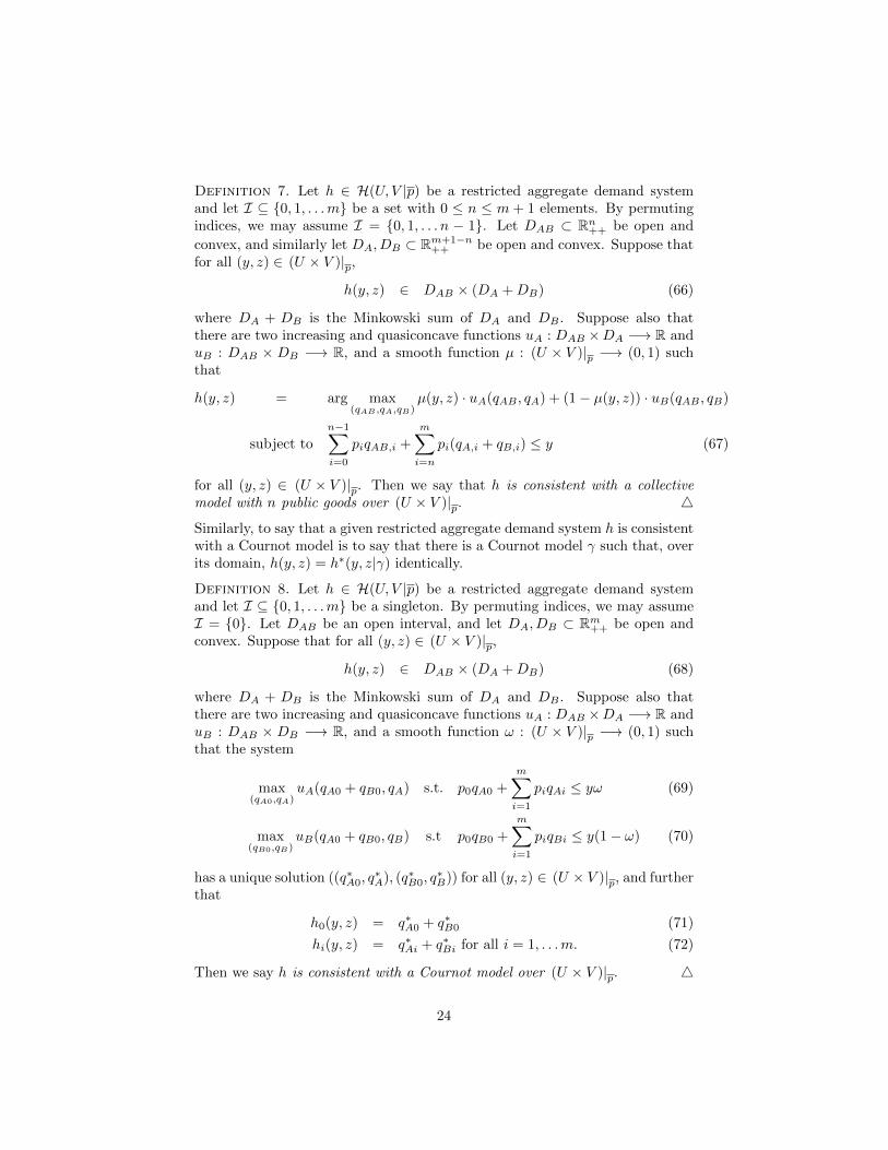
Definition 7. Let h ∈ H(U, V |p) be a restricted aggregate demand systemand let I ⊆ {0, 1, . . .m} be a set with 0 ≤ n ≤ m + 1 elements. By permutingindices, we may assume I = {0, 1, . . . n − 1}. Let DAB ⊂ Rn++ be open and
convex, and similarly let DA, DB ⊂ Rm+1−n++ be open and convex. Suppose that
for all (y, z) ∈ (U × V )|p,
h(y, z) ∈ DAB × (DA +DB) (66)
where DA + DB is the Minkowski sum of DA and DB . Suppose also thatthere are two increasing and quasiconcave functions uA : DAB ×DA −→ R anduB : DAB × DB −→ R, and a smooth function µ : (U × V )|p −→ (0, 1) suchthat
h(y, z) = arg max(qAB ,qA,qB)
µ(y, z) · uA(qAB , qA) + (1− µ(y, z)) · uB(qAB , qB)
subject to
n−1∑i=0
piqAB,i +
m∑i=n
pi(qA,i + qB,i) ≤ y (67)
for all (y, z) ∈ (U × V )|p. Then we say that h is consistent with a collectivemodel with n public goods over (U × V )|p. 4
Similarly, to say that a given restricted aggregate demand system h is consistentwith a Cournot model is to say that there is a Cournot model γ such that, overits domain, h(y, z) = h∗(y, z|γ) identically.
Definition 8. Let h ∈ H(U, V |p) be a restricted aggregate demand systemand let I ⊆ {0, 1, . . .m} be a singleton. By permuting indices, we may assumeI = {0}. Let DAB be an open interval, and let DA, DB ⊂ Rm++ be open andconvex. Suppose that for all (y, z) ∈ (U × V )|p,
h(y, z) ∈ DAB × (DA +DB) (68)
where DA + DB is the Minkowski sum of DA and DB . Suppose also thatthere are two increasing and quasiconcave functions uA : DAB ×DA −→ R anduB : DAB × DB −→ R, and a smooth function ω : (U × V )|p −→ (0, 1) suchthat the system
max(qA0,qA)
uA(qA0 + qB0, qA) s.t. p0qA0 +m∑i=1
piqAi ≤ yω (69)
max(qB0,qB)
uB(qA0 + qB0, qB) s.t p0qB0 +
m∑i=1
piqBi ≤ y(1− ω) (70)
has a unique solution ((q∗A0, q∗A), (q∗B0, q
∗B)) for all (y, z) ∈ (U × V )|p, and further
that
h0(y, z) = q∗A0 + q∗B0 (71)
hi(y, z) = q∗Ai + q∗Bi for all i = 1, . . .m. (72)
Then we say h is consistent with a Cournot model over (U × V )|p. 4
24
Define, for each possible domain (U × V )|p, the family of demand systems
H(n)0 (U, V |p) = {h ∈ H(U, V |p) : h is consistent with a collective model with n public goods}. (73)
Their union is the set of demand systems which are consistent with at least onecollective model:
H0(U, V |p) =
m+1⋃n=0
H(n)0 (U, V |p). (74)
Also define the set of demand systems which are consistent with at least oneCournot model:
H1(U, V |p) = {h ∈ H(U, V |p) : h is consistent with a Cournot model}. (75)
I will show that H0(U, V |p) and H1(U, V |p) are not well-separated, in the fol-lowing sense:
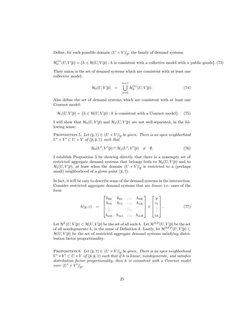
Proposition 5. Let (y, z) ∈ (U × V )|p be given. There is an open neighborhoodU ′ × V ′ ⊂ U × V of (p, y, z) such that
H0(U ′, V ′|p) ∩H1(U ′, V ′|p) 6= ∅. (76)
I establish Proposition 5 by showing directly that there is a nonempty set ofrestricted aggregate demand systems that belongs both to H0(U, V |p) and toH1(U, V |p), at least when the domain (U × V )|p is restricted to a (perhapssmall) neighborhood of a given point (y, z).
In fact, it will be easy to describe some of the demand systems in the intersection.Consider restricted aggregate demand systems that are linear, i.e. ones of theform
h(y, z) =
h00 h01 . . . h0Kh10 h11 . . . h1K
.... . .
hm0 hm1 . . . hmK
×yz1...zK
. (77)
LetHL(U, V |p) ⊂ H(U, V |p) be the set of all such h. LetHND(U, V |p) be the setof all nondegenerate h, in the sense of Definition 3. Lastly, let HDFP (U, V |p) ⊂H(U, V |p) be the set of restricted aggregate demand systems satisfying distri-bution factor proportionality.
Proposition 6. Let (y, z) ∈ (U × V )|p be given. There is an open neighborhoodU ′×V ′ ⊂ U ×V of (p, y, z) such that if h is linear, nondegenerate, and satisfiesdistribution factor proportionality, then h is consistent with a Cournot modelover (U ′ × V ′)|p.
25
Proof. See Appendix A.
Proposition 7. Let (y, z) ∈ (U × V )|p be given. There is an open neighborhoodU ′×V ′ ⊂ U ×V of (p, y, z) such that if h is linear, nondegenerate, and satisfiesdistribution factor proportionality, then h is consistent with a collective modelover (U ′ × V ′)|p.
Proof. See Appendix A.
Proof of Proposition 5. Proposition 6 shows that
HL(U ′, V ′|p) ∩HND(U ′, V ′|p) ∩HDFP (U ′, V ′|p) ⊂ H1(U ′, V ′|p). (78)
But Proposition 7 shows that
HL(U ′, V ′|p) ∩HND(U ′, V ′|p) ∩HDFP (U ′, V ′|p) ⊂ H0(U ′, V ′|p) (79)
too. Examples 1 and 3 provide examples of restricted aggregate demand systemsinHL(U, V ′|p)∩HND(U, V ′|p)∩HDFP (U, V ′|p), regardless of the domain. Thus,
HL(U ′, V ′|p) ∩HND(U ′, V ′|p) ∩HDFP (U ′, V ′|p) 6= ∅. (80)
So we have H0(U ′, V ′|p) ∩H1(U ′, V ′|p) 6= ∅, as required.
Since distribution factors very rarely have a natural scale, arguments for usingglobal information about the relationship between the distribution factors andhousehold consumption patterns to identify inefficiency are bound to be some-what contrived. So even though Proposition 5 is only local in nature, it stillseverely constrains the use of variation in distribution factors alone to identifyinefficiency.
6 Restoring Identifiability
But inefficiency is a well-defined concept, even if its presence is not detectablein some settings. What Proposition 5 shows is that with no restrictions onpreferences or the allocative mechanisms ω and µ, there are demand systemsthat are consistent with both efficient and inefficient models. So to construct auseful test of efficiency, it will be necessary to restrict the class of models underconsideration, or to obtain data that is in some sense “richer”.
6.1 Disaggregated Data
In particular, suppose that ω, A’s effective share of household wealth, is ob-served. This might be the case if, rather than just aggregate wealth y, theeconometrician observes the pair (yA, yB), where yA is A’s legally defined wealthand yB is B’s. If the econometrician is willing to assume that property rightswithin the household perfectly reflect those external legal arrangements, then
26
he also knows ω = yA/(yA + yB).
However, this particular empirical specification of ω may be inappropriate inmany contexts; and whenever the law is unclear or loosely enforced, or assetsare jointly owned, this approach may not even be feasible. In those situations,which arguably apply to the majority of the world’s population, learning aboutω might be possible by collecting information about local gender norms or al-locative practices, as in [Udry, 1996] and [Goldstein & Udry, 2008].
In keeping with the nonparametric spirit of Section 5, consider demand sys-tems h(y, ω, z). As before, the problem is to find properties of the demandh∗∗(y, µ(y, ω, z)) generated by efficient models that are not also properties of thedemand h∗(y, ω) generated by Cournot models. (Collective models are silent onthe determinants of µ, so it is possible that ω is an argument of µ.)
Clearly, if distribution factors z are found to affect demand conditional on theintrahousehold property rights ω, then the noncooperative models of Section3 cannot be valid. But that would simply re-open the basic question of thispaper: is there a class of inefficient models against which the collective modelis identified?
Instead, I will proceed under the assumption that demand is a function of (y, ω)alone, and provide partial restrictions on preferences, and on the distribution ofω, under which it is possible to identify inefficiency. That is, suppose the demandsystem h : W −→ Rm+1
++ were known over some open domain W ⊂ R++× (0, 1),and that it satisfied
m∑i=0
hi(y, ω) = y (81)
for all (y, ω) ∈W . Would it be possible to reject efficiency on the basis of thatknowledge? If some information about the distribution of consumption is avail-able, and preferences satisfy a certain asymmetry in income effects, it is indeedpossible.
Say we can classify some of the household’s expenditures as being either pub-lic, exclusively consumed by A, or exclusively consumed by B. In particular,suppose that the econometrician knows that good i = 0 is public, that good1 is privately consumed by A alone, and good 2 is privately consumed by Balone. This is not a complete disaggregation of consumption, but it is moreinformation than is typically used in the literature.
Assume that the preferences of both parties for the private goods are separablefrom the public good, so that uA and uB are of the form
uA(q0, qA) = uA(q0, vA(qA)) (82)
uB(q0, qB) = uA(q0, vB(qB)) (83)
27
and that the functions vA and vB are homogenous of degree one. Also assumethat the assignable private goods 1 and 2 satisfy an Inada condition, so
limq1→0+
∂uA∂qA1
(q0, qA) = +∞ (84)
limq2→0+
∂uB∂qB2
(q0, qB) = +∞. (85)
Further, assume that for all efficient allocations (q∗∗0 , q∗∗A , q∗∗B ),
∂
∂vA
(∂uA/∂q0∂uA/∂vA
(q∗∗0 , vA(q∗∗A ))
)6= ∂
∂vB
(∂uB/∂q0∂uB/∂vB
(q∗∗0 , vB(q∗∗B ))
).(86)
Finally, I will restrict the set of collective models by assuming that for all y, thePareto weight function µ(y, ω) is surjective. That is, for any µ ∈ (0, 1), there issome ω ∈ (0, 1) such that µ(y, ω) = µ.
With these restrictions on preferences and the set of collective models, a large-support condition on ω will be enough to identify inefficiency. Let y be givenand recall that the physical units of the goods are chosen such that all pricesare unity. Then we have
Proposition 8. Suppose A and B’s preferences for the private goods are sep-arable from the public good, their preferences for the private goods are homoge-nous of degree one, and their preferences for the assignable goods satisfy theInada conditions (84)-(85). Suppose also that the support of the conditionaldistribution of ω at y is the full unit interval: inf{ω : (y, ω) ∈ W} = 0, andsup{ω : (y, ω) ∈W} = 1. Let
ω = arg inf h0(y, ω) (87)
Then for any collective model such that µ(y, ω) is surjective at y,
min{h1(y, ω), h2(y, ω)} = 0. (88)
Proof. See Appendix A.
Importantly, the condition (88) is both testable and not true of Cournot models.Figure 1 illustrates the logic of this result: in noncooperative households, thelowest level of public consumption occurs when the distribution of effectivewealth ω is relatively equal, meaning that neither agent’s private consumptionwill be zero. In cooperative households, the lowest level of public consumptionoccurs when the partner who cares least about the public good has all thebargaining power, meaning the other agent’s private consumption has to bezero.
Proposition 9. Suppose A and B’s preferences for the private goods are sep-arable from the public good, their preferences for the private goods are homoge-nous of degree one, and their preferences for the assignable goods satisfy the
28
Inada conditions (84)-(85). Suppose also that the support of the conditionaldistribution of ω at y is the full unit interval: inf{ω : (y, ω) ∈ W} = 0, andsup{ω : (y, ω) ∈W} = 1. Let
ω = arg inf h0(y, ω) (89)
Then for any Cournot model,
min{h1(y, ω), h2(y, ω)} > 0. (90)
Proof. See Appendix A.
6.2 Preference Restrictions
Another route to identification is to restrict the preferences of the householdmembers. If we were willing to go so far as to fully specify both members’preferences, we could directly compute the efficient and the equilibrium alloca-tions. Testing a collective model against a Cournot one would then reduce tothe question of which model provides a better fit to the data. In fact, the iden-tification problem discussed in this paper is as much the fault of the completelack of restrictions on preferences as it is the fault of limited data on individualconsumption.
[Chiappori & Ekeland, 2009] show, in a similar setting to mine, that household-level data with price variation cannot identify the preferences of a household’smembers even within the class of collective models. In view of those results, thefailure of identification I establish should not be surprising. Without restrict-ing the permissible class of preferences for the household’s members beyondsome weak nonsatiation and convexity requirements, both efficient and inef-ficient models of the family are very “high-dimensional” objects, so it is notsurprising that it is hard to identify them from household-level data where bothmembers face the same prices.
7 Conclusion
Instead of looking for testable implications of intrafamily efficiency, it may bemore fruitful to look for the implications of inefficiency. Doing so entails takinga stand on what “efficiency” means, but the negative results of this paper showhow high the costs of being completely agnostic - about preferences, and aboutdecision mechanisms - are. Determining whether families are efficient at provid-ing public goods, such as children or housing, requires more information aboutpeople’s preferences for those goods than economists have thus far brought tobear on the question.
On theoretical grounds, one might be skeptical of the idea that inefficienciescan persist in the sort of long-term partnership that is family life. But the
29
inefficiencies described in this paper consist only of waste relative to a first-best allocation within an existing marriage, so it is easy to imagine that searchfrictions, or divorce costs, may make it individually rational to tolerate somefree-riding.
However, it remains to be seen whether the equilibrium matching patterns im-plied by an inefficient model of the family differ from those implied by an efficientone. Merging the analysis of decisions along the “extensive margin” of house-hold formation with those along the “intensive margin” - of allocation withinthe household - may be a useful direction for economists studying the family totake.
A Proofs of Propositions
A.1 Proofs for Section 3
Proof of Proposition 2. Let qA0(y(1− ω)|p) solve
qA0 = qB0(y(1− ω) + qA0) (91)
and similarly let qB0(yω|p) solve
qB0 = qA0(yω + qB0) (92)
If B’s contribution to the public good, qB0, is greater than qB0(yω|p), A will notcontribute, and similarly qA0 ≥ qA0(y(1− ω)|p) implies that B’s best responseis to free-ride by setting qB0 = 0.
Define ω∗(p, y) and ω∗(p, y) as the unique solutions to
qB0((1− ω∗)y|p) = qB0(yω|p) (93)
qA0(ω∗y|p) = qA0(y(1− ω)|p) (94)
Now, if ω is such that A does not contribute, then
qB0((1− ω)y|p) ≥ qB0(yω|p) (95)
but since qB0((1 − ω)y|p) is decreasing in ω and qB0(yω|p) is increasing in ω,we must have ω ≤ ω∗. Similar reasoning implies that B does not contribute -qB0 = 0 - exactly when A is sufficiently rich: ω ≥ ω∗. Finally, ω∗ < ω∗ becauseotherwise there would exist ω ∈ [ω∗, ω∗], but for such an ω, neither A nor Bwould contribute to the public good, and that cannot be an equilibrium. Butthis contradicts Theorem 2 of [Bergstrom et al. , 1986], which establishes thatin this game, an equilibrium always exists.
30
A.2 Proofs for Section 5
Proposition 2 shows that in equilibria where only one partner - say A - con-tributes to the public good, aggregate consumption of the public good is simplyq∗A0, and aggregate consumption of all the m private goods is q∗Aj + q∗Bj , forall j 6= 0. To prove Proposition 6, I reverse-engineer that equilibrium outcomelocally by finding a good i - say it is good 0 - and a scalar a ∈ (0, 1) and definingω(y, z) by the relation h0(y, z) = aω(y, z), so A’s Engel curve for the “public”good is linear by construction.
Then, I decompose the consumption of the remaining m goods as
hj(y, z) = qAj(ω(y, z)) + qBj(1− ω(y, z)) (96)
for 2m weakly positive, weakly increasing functions qAj and qBj such that“adding-up” holds:
aω(y, z) +
m∑j=1
qAj(ω(y, z)) = ω(y, z) (97)
m∑j=1
qBj(1− ω(y, z)) = 1− ω(y, z) (98)
Finally, I construct preferences uA, uB such that A and B’s Engel curves areexactly qAj and qBj for all the “private” goods 1 ≤ j ≤ m, and such that B doesnot contribute in equilibrium. This is always possible, I show, if B’s preferencefor the public good is weak enough.
Lemma 1. Let h : R2 −→ Rm+1 be given by
h(y, s) =
h00 h01h10 h11
...hm0 hm1
×[ys
]. (99)
Suppose also that for all i, hi0 > 0, hi1 6= 0, and
1 =
m∑i=0
hi0 (100)
0 =
m∑i=0
hi1. (101)
Then there is an integer i, 0 ≤ i ≤ m, a scalar a ∈ (0, 1), and a smooth function
31
ω : R2 −→ R such that (by permuting indices such that i = 0),
h(y, s) =
a 0δA1 δB1...δAm δBm
×[
yω(y, s)y(1− ω(y, s))
](102)
for all (y, s) ∈ R2. Furthermore, the constants δAj , δBj can be chosen to be
nonnegative and such that
m∑j 6=i
δAj = 1− a (103)
m∑j 6=i
δBj = 1. (104)
Proof of Lemma 1. Since all hj1 are nonzero, partition {0, 1 . . .m} into
J + = {j : hj1 > 0} (105)
J− = {j : hj1 < 0}. (106)
Both J + and J− are nonempty, because∑mj=0 hj1 = 0. Let
i ∈ arg min
{hj0hj1
: j ∈ J +
}. (107)
and define, for all j 6= i,
δBj = hj0 − hi0hj1hi1
(108)
δAj = δBj + ahj1hi1
= hj0 + (a− hi0)hj1hi1
(109)
for an a ∈ (0, 1) that is, for now, unspecified. By construction, δBj ≥ 0 for all
j ∈ J +, and clearly δBj ≥ 0 for j ∈ J−. This implies that if j ∈ J +, then
δAj ≥ 0 whenever a ≥ 0. Now, suppose that for all j ∈ J−
a ≤ hi0 − hj0hi1hj1
= hi0 + hj0
∣∣∣∣hi1hj1
∣∣∣∣ (110)
If so, then for all j ∈ J−,
δAj = hj0 + (a− hi0)hj1hi1
= hj0 − (a− hi0)
∣∣∣∣hj1hi1
∣∣∣∣ ≥ 0. (111)
32
So, let a be such that
0 < a < min
{1, hi0 + hi1 · min
j∈J−
∣∣∣∣hj0hj1
∣∣∣∣} (112)
Define
ω(y, s) =1
ayhi(y, s). (113)
For any j 6= i,
hj(y, s) = y · hj0 + s · hj1
= y · hj0 + hj1 ·1
hi1[ayω(y, s)− y · hi0]
= y ·{[hj0 − hi0 ·
hj1hi1
]+
[ahj1hi1
]ω(y, s)
}= y ·
{[hj0 − hi0 ·
hj1hi1
]· [(1− ω(y, s)) + ω(y, s)] +
[ahj1hi1
]ω(y, s)
}= δAj · yω(y, s) + δBj · y(1− ω(y, s)). (114)
Corollary 2. Let h(y, s) be as in Lemma 1 above. If y > 0, a can be chosensuch that ω(y, 0) ∈ (0, 1).
Proof. If we choose a such that
0 < hi0 < a < min
{1, hi0 + hi1 · min
j∈J−
∣∣∣∣hj0hj1
∣∣∣∣} (115)
then
ω(y, 0) =1
ayhi(y, 0)
=hi0a
< 1. (116)
Proof of Proposition 6. Let h ∈ HL(U, V |p)∩HND(U, V |p)∩HDFP (U, V |p) begiven by
h(y, z) =
h00 h01 . . . h0Kh10 h11 . . . h1K
.... . .
hm0 hm1 . . . hmK
×yz1...zK
. (117)
33
Because h is nondegenerate, hik 6= 0 for all goods i. And because distributionfactors have no natural scale, is without loss of economic generality to assumez = 0. h satisfies adding-up, so for any y,
m∑i=0
hi(y, z) =
(m∑i=0
hi0
)y
= y (118)
which means∑mi=1 hi0 = 1. Then because budget shares are strictly positive,
hi(y, z)/y = hi0 > 0. But again by adding up,
m∑i=0
hi(0, z) =
m∑i=1
K∑k=1
hikzk
= 0. (119)
By considering z = (1, 0, . . . 0), we see that∑mi=0 hi1 = 0.
Next, let
s(z) =
K∑k=1
hikhi1
zk. (120)
Because h satisfies distribution factor proportionality, the ratio hik/hi1 does notdepend on the choice of good i, so s is well-defined.
For all goods i, and all (y, z) ∈ (U × V )|p, then,
hi(y, z) = y · hi0 + hi1
K∑k=1
hikhi1
zk
= y · hi0 + hi1 · s(z). (121)
By Lemma 1, we can express the demand system h as
h0(y, z) = a · yω(y, s(z)) (122)
and for all j 6= 0,
hj(y, z) = δAj · yω(y, s(z)) + δBj · y(1− ω(y, s(z))). (123)
By Corollary 2, we can choose a such that ω(y, s(z)) ∈ (0, 1). Let
G ={
(y, z) ∈ (U × V )|p : ω(y, z) ∈ (0, 1)}. (124)
34
G is open, because ω is continuous. Let
yA
= inf(y,z)∈G
yω(y, z) (125)
yB
= inf(y,z)∈G
y(1− ω(y, z)) (126)
ω = inf(y,z)∈G
ω(y, z) (127)
yA = sup(y,z)∈G
yω(y, z) (128)
yB = sup(y,z)∈G
y(1− ω(y, z)) (129)
ω = sup(y,z)∈G
ω(y, z) (130)
and define
DAB = (ayA, ayA) (131)
DA =
m∏j=1
(δAj · yA, δAj · yA) (132)
DB =
m∏j=1
(δBj · yB , δBj · yB). (133)
If any of the δAj or δBj are zero, we may replace (δAj ·yA, δAj ·yA) = ∅ with (0,∞),
so that DA and DB remain open and convex. Finally, let
uA(q0, qA) = a log(q0) +
m∑j=1
δAj log(qAj) (134)
uB(q0, qB) = b log(q0) + (1− b) ·m∑j=1
δBj log(qBj) (135)
for some b > 0 such that
b <a · ω
(1− ω) + a · ω(136)
so that for all (y, z) ∈ G,
ω(y, z) ≥ ω
>b
a+ (1− a)b(137)
which implies
b[(1− ω(y, z)) + aω(y, z)] < aω(y, z) (138)
so that B will not contribute in equilibrium. Thus, h meets Definition 8, and isconsistent with a Cournot model.
35
Proof of Proposition 7. As in the proof of Proposition 6, decompose h as
h0(y, z) = a · yω(y, s(z)) (139)
and for all j 6= 0,
hj(y, z) = δAj · yω(y, s(z)) + δBj · y(1− ω(y, s(z))). (140)
but let
uA(q0, qA) = a log(q0) +
m∑j=1
δAj log(qAj) (141)
uB(q0, qB) =
m∑j=1
δBj log(qBj). (142)
Then h meets Definition 7, and is consistent with a collective model with nopublic goods.
A.3 Proofs for Section 6
Proof of Proposition 8. Since (p, y) is fixed, I suppress the dependence of allfunctions on those variables. The demand system is a set of m + 1 functionshi : (0, 1) −→ (0, 1) such that
∑mi=0 hi(ω) = 1 for all ω ∈ (0, 1).
If h is generated by a collective model, then h(ω) = h∗∗(µ(ω)) for some functionµ(ω), where
h∗∗(µ) = arg maxµ · uA(q0, vA(qA)) + (1− µ) · uB(q0, vB(qB))
s.t. q0 +
m∑i=0
(qAi + qBi) ≤ y. (143)
Suppose h∗∗0 (µ) were strictly monotone in µ. Note that because µ(·) is surjectiveand the support of ω is the entire unit interval [0, 1], supω∈(0,1) µ(ω) = 1 and
infω∈(0,1) µ(ω) = 0. Then, letting µ = (h∗∗0 )−1(h0(ω)), we have µ ∈ {0, 1}.That is, the minimum consumption of the public good occurs when one partnerhas no bargaining power at all. But then that partner must have zero privateconsumption, too, so
min{h1(y, ω), h2(y, ω)} = 0. (144)
To show that the collective demand for the public good h∗∗0 (µ) is monotone inµ, let
qA = arg max vA(qA) s.t.
m∑i=1
qAi ≤ 1 (145)
vA = vA(qA) (146)
qB = arg max vB(qB) s.t.
m∑i=1
qBi ≤ 1 (147)
vB = vB(qB) (148)
36
The separability assumptions on uA and uB and homogeneity assumptions onvA and vB mean that the set of efficient private consumption vectors q∗∗A , q
∗∗B
lies in a subspace of Rm of dimension at most two: that is, any efficient al-location (q∗∗0 , q∗∗A , q
∗∗B ) must be of the form (q∗∗0 , x∗∗A · qA(1), xB · qB(1)), where
q∗∗0 + x∗∗A + x∗∗B = y.
I will show that ddµh
∗∗0 (µ) 6= 0 for all µ, which by continuity will imply that
h∗∗0 is monotone. Suppose there were some µ such that ddµh
∗∗0 (µ) = 0, and let
(q∗∗0 , x∗∗A · qA, x∗∗B · qB) be the efficient allocation corresponding to µ. Thus,
∂uA/∂q0∂uA/∂vA
(q∗∗0 , x∗∗A vA) · 1
vA+∂uB/∂q0∂uB/∂vB
(q∗∗0 , x∗∗B vB) · 1
vB= 1. (149)
Then for a small change dx in the allocation of private expenditures, (q∗∗0 , (x∗∗A +dx) · qA, (x∗∗B − dx) · qB) would be efficient, and we would also have
∂uA/∂q0∂uA/∂vA
(q∗∗0 , (x∗∗A + dx)vA) · 1
vA+∂uB/∂q0∂uB/∂vB
(q∗∗0 , (x∗∗B − dx)vB) · 1
vB= 1.(150)
Subtracting (149) from (150) and letting dx → 0, we have that ddµh
∗∗0 (µ) = 0
implies that
∂
∂vA
(∂uA/∂q0∂uA/∂vA
(q∗∗0 , vA(q∗∗A ))
)=
∂
∂vB
(∂uB/∂q0∂uB/∂vB
(q∗∗0 , vB(q∗∗B ))
)(151)
which contradicts (86).
Proof of Proposition 9. By Proposition 2, the minimum expenditure on the pub-lic good occurs at ω ∈ (ω∗, ω
∗), but 0 < ω∗ < ω∗ < 1. If the distribution ofincome is interior, neither A nor B will have zero private consumption, so
min{h1(y, ω), h2(y, ω)} > 0. (152)
B Efficiency Loss in a CES Cournot Model
B.1 Defining the Efficiency Loss
Let (q∗0 , q∗A, q∗B) be the equilibrium allocation for the Cournot model. Define the
equilibrium utilities
u∗A(ω|p, y) = uA(q∗0(ω|p, y), q∗A(ω|p, y)) (153)
u∗B(ω|p, y) = uB(q∗0(ω|p, y), q∗B(ω|p, y)) (154)
37
Consider a social planner’s cost-minimization problem, given a profile of utilities(uA, uB)
c∗∗(uA, uB |p) = min(q0,qA,qB)
q0 + p(qA + qB) (155)
s.t. uA(q0, qA) ≥ uAuB(q0, qB) ≥ uB
What I will call the “efficiency loss,” d, is the relative difference between thesocial planner’s minimized cost of achieving the utilities that agents enjoy inequilibrium, and the total resources in the household:
d(ω|p, y) = 1− c∗∗(u∗A(ω|p, y), u∗B(ω|p, y))|p)y
(156)
One way to interpret d is as the compensating variation associated with an ex-ogenous move to the Lindahl prices that give A and B their equilibrium utilities(or, more poetically, a move to Coasian bargaining). Stated differently, it is Aand B’s aggregate willingness to pay to hire a social planner.7
In the following section, I provide explicit formulae for a quadratic approxi-mation to d(ω|p, y) when both agents have constant-elasticity-of-substitution(CES) preferences.
B.2 A “Harberger Triangle” for the Cournot Model
Let us rewrite the problem (155) in one dimension: define qA(q0, u∗A(ω|p, y))
and qB(q0, u∗B(ω|p, y)) implicitly by
u∗A(ω|p, y) = uA(q0, qA) (157)
u∗B(ω|p, y) = uB(q0, qB) (158)
and let
c(q0) = q0 + p(qA(q0, u∗A(ω|p, y)) + qB(q0, u
∗B(ω|p, y))) (159)
Let q∗∗0 be the socially optimal quantity of the public good, i.e. the value of q0that minimizes (159). Obviously, c(q∗0(ω|p, y)) = y, and
c(q∗∗0 ) = c∗∗(u∗A(ω|p, y), u∗B(ω|p, y)|p))= y(1− d(ω|p, y)) (160)
7When both partners have homothetic preferences, it can be shown thatc∗∗(u∗A(ω|p, y), u∗B(ω)|p, y) is homogenous of degree one in (uA, uB), and thus the effi-ciency loss d is homogenous of degree zero in (yA, yB) = (yω, y(1 − ω)). In that situation,there is no loss of generality in setting yA + yB = 1. Moreover, the envelope theorem andRoy’s identity imply that c∗∗(u∗A(ω|p, y), u∗B(ω|p, y)) is locally constant in p (except whenvariations in p, for constant y, changes the set of equilibrium contributors to the publicgood), so that d depends only on the effective share of the endowment ω, but not on prices p.
38
In general, d(ω|p, y) must be calculated numerically. However, a useful shortcutis to take a quadratic approximation to the social planner’s cost function (159)about q∗∗0 . Doing so leads to the following version of a Harberger triangle:
Proposition 10. The equilibrium efficiency loss is
d(ω|p, y)− 1
2
[c′(q∗0)]2
(yA + yB)c′′(q∗0)= O
((q∗0 − q∗∗0 )2
). (161)
It remains to calculate the first and second derivatives c′(q∗0) and c′′(q∗0). As ashorthand, let
MRS(q∗0 , u∗A) =
∂uA/∂q0∂uA/∂qA1
(q∗0 , q∗A1) (162)
be A’s marginal willingness to pay for the public good at the Cournot equilib-rium. Then the the numerator in (161) is
c′(q∗0) = 1 + p
(∂qA∂q0
+∂qB∂q0
)= 1− p (MRS(q∗0 , u
∗A) +MRS(q∗0 , u
∗B)) (163)
By construction, the first derivative c′ is the difference between the relative priceof the public good and the sum of A and B’s marginal rates of substitution, i.e.the marginal social willingness to pay for the public good. The efficiency lossis therefore approximately quadratic in the marginal distortion in equilibrium,echoing the familiar analysis of the deadweight loss of taxation.
When both partners have constant-elasticity of substitution (CES) preferences,i.e.
uA(q0, qA1) = (aqρA0 + (1− a)qρAA1)1/ρA (164)
uB(q0, qB1) = (bqρB0 + (1− b)qρBB1)1/ρB (165)
the first derivative c′(q∗0) in (163) becomes
c′(q∗0) = 1− p
[(a
1− a
)(q∗0q∗A
)ρA−1+
(b
1− b
)(q∗0q∗B
)ρB−1](166)
Obtaining the denominator c′′(q∗0) takes more work, but is not complicated.Note that A’s marginal willingness to pay for q0 is exactly
MRS(q∗0 , u∗A) =
1
p(q∗0 , u∗A)
(167)
where p(q0, u) is A’s inverse Hicksian demand for q0. Then
c′′(q∗0) = −p[
1
[p(q∗0 , u∗A)]2
∂p(q∗0 , u∗A)
∂q0+
1
[p(q∗0 , u∗B)]2
∂p(q∗0 , u∗B)
∂q0
](168)
39
Assembling the components of (168), we have A’s Hicksian demand given by
qH0 (p, u) = u · aσA ·[aσA + (1− a)σAp1−σA
] σA1−σA (169)
where, as usual, we let σA = (1−ρA)−1 and σB = (1−ρB)−1 denote A and B’selasticities of substitution between the private and public goods.
Then,
p(q0, u∗A) =
(a
1− a
) σA1−σA
[1
a(u∗A)
σA−1
σA q1−σAσA
0 − 1
] 11−σA
(170)
Differentiating, we obtain (after some algebra)
∂p(q0, u∗A)
∂q0=
1
σAq0
[p(q0, u
∗A) +
(a
1− a
)σAp(q0, u
∗A)σA
](171)
Repeating the analogous calculations for B and substituting in (168), we finallyarrive at
c′′(q∗0) =p
q∗0
{1
σA
(MRSA(q∗0 , u
∗A) +
[a
1− a
]σAMRSA(q∗0 , u
∗A)2−σA
)+
1
σB
(MRSB(q∗0 , u
∗B) +
[b
1− b
]σBMRSB(q∗0 , u
∗B)2−σB
)}(172)
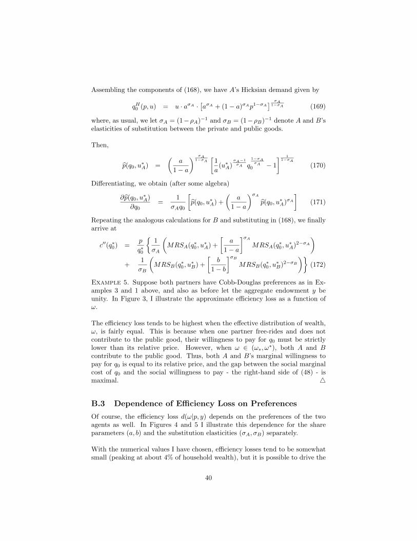
Example 5. Suppose both partners have Cobb-Douglas preferences as in Ex-amples 3 and 1 above, and also as before let the aggregate endowment y beunity. In Figure 3, I illustrate the approximate efficiency loss as a function ofω.
The efficiency loss tends to be highest when the effective distribution of wealth,ω, is fairly equal. This is because when one partner free-rides and does notcontribute to the public good, their willingness to pay for q0 must be strictlylower than its relative price. However, when ω ∈ (ω∗, ω
∗), both A and Bcontribute to the public good. Thus, both A and B’s marginal willingness topay for q0 is equal to its relative price, and the gap between the social marginalcost of q0 and the social willingness to pay - the right-hand side of (48) - ismaximal. 4
B.3 Dependence of Efficiency Loss on Preferences
Of course, the efficiency loss d(ω|p, y) depends on the preferences of the twoagents as well. In Figures 4 and 5 I illustrate this dependence for the shareparameters (a, b) and the substitution elasticities (σA, σB) separately.
With the numerical values I have chosen, efficiency losses tend to be somewhatsmall (peaking at about 4% of household wealth), but it is possible to drive the
40
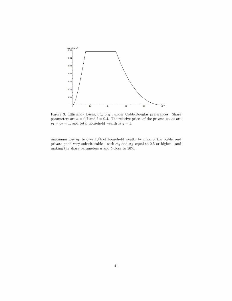
Figure 3: Efficiency losses, d(ω|p, y), under Cobb-Douglas preferences. Shareparameters are a = 0.7 and b = 0.4. The relative prices of the private goods arep1 = p2 = 1, and total household wealth is y = 1.
maximum loss up to over 10% of household wealth by making the public andprivate good very substitutable - with σA and σB equal to 2.5 or higher - andmaking the share parameters a and b close to 50%.
41
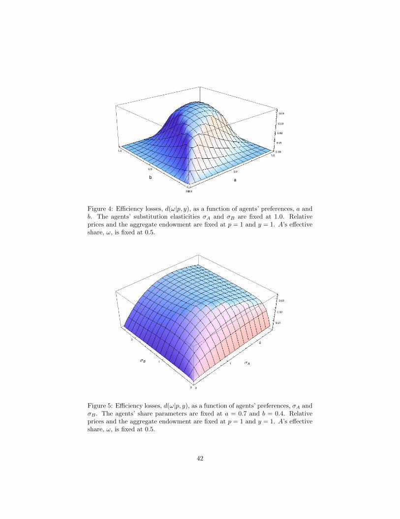
Figure 4: Efficiency losses, d(ω|p, y), as a function of agents’ preferences, a andb. The agents’ substitution elasticities σA and σB are fixed at 1.0. Relativeprices and the aggregate endowment are fixed at p = 1 and y = 1. A’s effectiveshare, ω, is fixed at 0.5.
Figure 5: Efficiency losses, d(ω|p, y), as a function of agents’ preferences, σA andσB . The agents’ share parameters are fixed at a = 0.7 and b = 0.4. Relativeprices and the aggregate endowment are fixed at p = 1 and y = 1. A’s effectiveshare, ω, is fixed at 0.5.
42
C Implications of Efficiency In Data With PriceVariation: “SR1” Conditions
None of the following is original; it is simply a repetition of material from[Browning & Chiappori, 1998], included for completeness only.
Definition 9. Let g ∈ G(U, V ) be an extended aggregate demand system, andlet (p, y, z) ∈ U × V . If the “pseudo-Slutsky” matrix S(p, y, z), with (i, j)-thentry
sij(p, y, z) =∂gi∂pj
+ gj ·∂gi∂y
(173)
can be written as
S(p, y, z) = Σ(p, y, z) +R(p, y, z) (174)
for some negative semidefinite matrix Σ and some matrix R with rank(R) ≤ 1,then we say that g is negative semidefinite plus rank one at (p, y, z), or, as ashorthand, g is SR1 at (p, y, z).
Proposition 11. If the extended aggregate demand system g is induced by acollective model θ ∈ Θ(U, V ), then g is SR1 at all (p, y, z) ∈ U × V .
Proof. Since g is induced by a collective model θ = (I, uA, uB , µ), we can write
g(p, y, z) = g∗∗(p, y, µ(p, y, z)|θ) (175)
Differentiating (175) for any good i, we have
∂gi∂pj
=∂g∗∗i∂pj
+∂g∗∗i∂µ· ∂µ∂pj
(176)
∂gi∂y
=∂g∗∗i∂y
+∂g∗∗i∂µ· ∂µ∂y
(177)
(178)
so that
sij(p, y, z) =∂gi∂pj
+ gj ·∂gi∂y
=∂g∗∗i∂pj
+∂g∗∗i∂µ· ∂µ∂pj
+ g∗∗j
[∂g∗∗i∂y
+∂g∗∗i∂µ· ∂µ∂y
]=
{∂g∗∗i∂pj
+ g∗∗j ·∂g∗∗i∂y
}+∂g∗∗i∂µ·{∂µ
∂pj+ g∗∗j ·
∂µ
∂y
}(179)
The first term in the final line of (179) is the (i, j)-th entry in the Slutskymatrix of the demand function g∗∗(p, y, µ(p, y, z)), holding µ fixed. If it werepossible to observe demands by varying (p, y) without also varying the Pareto
43
weight µ, the result would be the constrained maximizer of the concave functionµ ·uA+[1−µ]uB . Thus, the matrix Σ with such entries is negative semidefinite.
The second term in (179) is the the (i, j)-th entry in the matrix
R =
∂g∗∗0∂µ∂g∗∗1∂µ...
∂g∗∗m∂µ
×[∂µ∂p0
+ g∗∗0∂µ∂y ,
∂µ∂p1
+ g∗∗1∂µ∂y , . . . ∂µ
∂pm+ g∗∗m
∂µ∂y
](180)
Since R is the outer product of two vectors, rank(R) ≤ 1.
Now, what if the pair (yA, yB) were observed, not just y = yA + yB? Thendemands would be a function of (p, yA, yB , z) rather than (p, y, z). We mightuse yA/(yA + yB) as an empirical measure of ω (in a noncooperative model), oras a component of z in a collective model.
Let φ ∈ [0, 1] be given; the analogue of the pseudo-Slutsky matrix (173) wouldhave (i, j)-th entry
sij(p, yA, yB |φ) = φ
{d
dpjgi(p, yA, yB) + gj(p, yA, yB)
d
dyAgi(p, yA, yB)
}+ (1− φ)
{d
dpjgi(p, yA, yB) + gj(p, yA, yB)
d
dyBgi(p, yA, yB)
}= gj(p, yA, yB)
{φd
dyAgi(p, yA, yB) + (1− φ)
d
dyBgi(p, yA, yB)
}+
d
dpjgi(p, yA, yB). (181)
Direct calculation of (181) for collective demands, i.e. demands of the formg∗∗(p, yA + yB , µ(p, yA, yB)) is SR1 for any weight φ.
But Theorem 4 of [Lechene & Preston, 2011] shows that the aggregate demandsg∗(p, yA+yB , yA/(yA+yB)) of a noncooperative household will obey these sameSR1 conditions, at least when each partner’s preferences for private goods areweakly separable from the public good. So the prospects for the identificationof inefficiency using SR1 conditions are not good, unless the particular form ofthese nonseparabilities are known.
References
[Alderman et al. , 1995] Alderman, H, Chiappori, P.A., Haddad, L, Hoddinott,J, & Kanbur, R. 1995. Unitary versus collective models of the household: is
44
it time to shift the burden of proof? The World Bank Research Observer,10(1), 1–19.
[Attanasio & Lechene, 2014] Attanasio, Orazio P, & Lechene, Valerie. 2014. Ef-ficient responses to targeted cash transfers. Journal of Political Economy,122(1), 178–222.
[Bayudan, 2006] Bayudan, Connie G. 2006. Wives’ time allocation and intra-household power: evidence from the Philippines. Applied Economics, 38(7),789–804.
[Becker, 1991] Becker, Gary S. 1991. A Treatise on the Family. 2nd edn. Cam-bridge, Massachusetts: Harvard University Press.
[Becker & Murphy, 1988] Becker, Gary S, & Murphy, Kevin M. 1988. The Fam-ily and the State. Journal of Law and Economics.
[Bergstrom et al. , 1986] Bergstrom, T, Blume, L, & Varian, H. 1986. On theprivate provision of public goods. Journal of Public Economics, 29(1), 25–49.
[Bobonis, 2009] Bobonis, Gustavo J. 2009. Is the allocation of resources withinthe household efficient? New evidence from a randomized experiment. Jour-nal of Political Economy, 117(3), 453–503.
[Bourguignon et al. , 2009] Bourguignon, F, Browning, M, & Chiappori, P.A.2009. Efficient intra-household allocations and distribution factors: Implica-tions and identification. The Review of Economic Studies, 76(2), 503–528.
[Bourguignon et al. , 1993] Bourguignon, Francois, Browning, Martin, Chiap-pori, Pierre-Andre, & Lechene, Valerie. 1993. Intra household allocationof consumption: A model and some evidence from French data. Annalesd’Economie et de Statistique, 137–156.
[Browning & Chiappori, 1998] Browning, M, & Chiappori, P.A. 1998. Efficientintra-household allocations: A general characterization and empirical tests.Econometrica: Journal of the Econometric Society, 1241–1278.
[Browning et al. , 1994] Browning, M, Bourguignon, F, Chiappori, P.A., &Lechene, V. 1994. Income and outcomes: A structural model of intrahouse-hold allocation. Journal of Political Economy, 1067–1096.
[Chen & Woolley, 2001] Chen, Zhiqi, & Woolley, Frances. 2001. A Cournot-Nash Model of Family Decision Making. The Economic Journal, 111(474),722–748.
[Cherchye et al. , 2007] Cherchye, Laurens, de Rock, Bram, & Vermeulen, Fred-eric. 2007. The Collective Model of Household Consumption: A Nonparamet-ric Characterization. Econometrica, 75(2), 553–574.
45
[Cherchye et al. , 2009] Cherchye, Laurens, de Rock, Bram, & Vermeulen, Fred-eric. 2009. Opening the black box of intrahousehold decision making: Theoryand nonparametric empirical tests of general collective consumption models.Journal of Political Economy, 117(6), 1074–1104.
[Chiappori, 1992] Chiappori, PA. 1992. Collective Labor Supply and Welfare.Journal of Political Economy, 437–467.
[Chiappori et al. , 2002] Chiappori, PA, Fortin, Bernard, & Lacroix, G. 2002.Marriage Market, Divorce Legislation, and Household Labor Supply. Journalof Political Economy, 110(1), 37–72.
[Chiappori & Ekeland, 2009] Chiappori, Pierre-Andre, & Ekeland, Ivar. 2009.The Microeconomics of Efficient Group Behavior: Identification. Economet-rica, 77(3), 763–799.
[Del Boca & Flinn, 2012] Del Boca, Daniela, & Flinn, Christopher. 2012. En-dogenous household interaction. Journal of Econometrics, 166(1), 49–65.
[Del Boca & Flinn, 2014] Del Boca, Daniela, & Flinn, Christopher J. 2014.Household behavior and the marriage market. Journal of Economic Theory,150, 515–550.
[Donni, 2007] Donni, O. 2007. Collective female labour supply: theory andapplication. The Economic Journal, 117(516), 94–119.
[Donni & Moreau, 2007] Donni, Olivier, & Moreau, Nicolas. 2007. CollectiveLabor Supply A Single-Equation Model and Some Evidence from FrenchData. Journal of Human Resources, 42(1), 214–246.
[Duflo, 2003] Duflo, Esther. 2003. Grandmothers and Graddaughters: Old AgePension and Intra-Household Allocation in South Africa. World Bank Eco-nomic Review, 17(1), 1–25.
[Fortin & Lacroix, 1997] Fortin, Bernard, & Lacroix, Guy. 1997. A Test of theUnitary and Collective Models of Labor Supply. The Economic Journal,107(443), 933–955.
[Goldstein & Udry, 2008] Goldstein, Markus, & Udry, Christopher. 2008. Theprofits of power: Land rights and agricultural investment in Ghana. Journalof Political Economy, 116(6), 981–1022.
[Lechene & Preston, 2011] Lechene, V., & Preston, I. 2011. Noncooperativehousehold demand. Journal of Economic Theory, 146(2), 504–527.
[Lise & Yamada, 2014] Lise, Jeremy, & Yamada, Ken. 2014. Household Sharingand Commitment: Evidence from Panel Data on Individual Expenditures andTime Use.
[Lundberg & Pollak, 1993] Lundberg, S, & Pollak, R A. 1993. Separate spheresbargaining and the marriage market. Journal of Political Economy, 988–1010.
46
[Lundberg et al. , 1997] Lundberg, Shelly, Pollak, Robert A, & Wales, Ter-ence J. 1997. Do Husbands and Wives Pool Their Resources? EvidenceFrom the UK Child Benefits. The Journal of Human Resources, 32, 463–480.
[Manser & Brown, 1980] Manser, M, & Brown, M. 1980. Marriage and House-hold Decision-Making: A Bargaining Analysis. International Economic Re-view, 21(1), 31–44.
[Mazzocco, 2007] Mazzocco, Maurizio. 2007. Household intertemporal be-haviour: A collective characterization and a test of commitment. The Reviewof Economic Studies, 74(3), 857–895.
[McElroy & Horney, 1981] McElroy, M B, & Horney, M J. 1981. Nash-bargained household decisions: Toward a generalization of the theory of de-mand. International Economic Review, 22(2), 333–349.
[Thomas, 1990] Thomas, Duncan. 1990. Intra-household resource allocation:An inferential approach. Journal of Human Resources, 635–664.
[Udry, 1996] Udry, Christopher. 1996. Gender, agricultural production, and thetheory of the household. Journal of Political Economy, 1010–1046.
[Vermeulen, 2005] Vermeulen, Frederic. 2005. And the winner is... An empir-ical evaluation of unitary and collective labour supply models. EmpiricalEconomics, 30(3), 711–734.
[Voena, 2010] Voena, A. 2010. Yours, Mine, and Ours: Do Divorce Laws Affectthe Intertemporal Behavior of Married Couples? Unpublished Manuscript.
47