The Probability Distribution of

Sea Surface Wind Speeds:

Effects of Variable Surface Stratification

and Boundary Layer Thickness

Adam Hugh Monahan(monahana@uvic.ca)

School of Earth and Ocean Sciences

University of VictoriaP.O. Box 3065 STN CSC

Victoria, BC, Canada, V8W 3V6

Submitted to Journal of Climate

March 30, 2009

1

Abstract

Air-sea exchanges of momentum, energy, and material substances, of fundamental

importance to the variability of the climate system, are mediated by the character of

turbulence in the atmospheric and oceanic boundary layers. Sea surface winds influ-

ence, and are influenced by, these fluxes. The probability density function (pdf) of sea

surface wind speeds p(w) is a mathematical object describing the variability of surface

winds which arises from the physics of the turbulent atmospheric planetary boundary

layer. Previous mechanistic models of the pdf of sea surface wind speeds have con-

sidered the momentum budget of an atmospheric layer of fixed thickness and neutral

stratification. The present study extends this analysis to consider the influence (in the

context of an idealised model) of boundary layer thickness variations and non-neutral

surface stratification on p(w). It is found that surface stratification has little direct

influence on p(w), while variations in boundary layer thickness bring the predictions of

the model into closer agreement with observations. Boundary layer thickness variabil-

ity influences the shape of p(w) in two ways: through episodic downwards mixing of

momentum into the boundary layer from the free atmosphere, and modulation of the

importance (relative to other tendencies) of turbulent momentum fluxes at the surface

and the boundary layer top. It is shown that the second of these influences dominates

over the first.

1

1 Introduction

Air-sea exchanges of momentum, energy, and material substances, of fundamental impor-

tance to the variability of the climate system, are mediated by the character of turbulence

in the atmospheric and oceanic boundary layers. Sea surface winds influence, and are influ-

enced by, these fluxes. Standard bulk parameterisations express air-sea fluxes as functions

of the surface wind speed averaged over the “main timescales” of atmospheric boundary-

layer turbulence (e.g. are “eddy-averaged”). For those fluxes depending linearly on surface

wind speed (e.g. heat and moisture, to a first approximation), fluxes averaged over longer

timescales, or over some spatial domain, are given by the bulk formulae in terms of the

averaged wind speed. However, for other fluxes (e.g. momentum, gases, aerosols) the non-

linear dependence on surface wind speed implies that the mean flux is not the flux associated

with the mean wind speed (e.g. Wanninkhof et al., 2002) A further complication arises in

the computation of fluxes spatially averaged over some domain (e.g. a General Circulation

Model (GCM) gridbox): in general, there is a difference between the area-averaged mean

wind speed and the magnitude of the mean vector wind (e.g. Mahrt and Sun, 1995). Ac-

curate computations of (space or time) average fluxes require the development of models of

the probability distribution of sea surface winds.

A new era in the study of sea surface winds was ushered in with the introduction of high

resolution (in both space and time), global-scale observations from the SeaWinds scatterom-

eter on the Quick Scatterometer (QuikSCAT) satellite (Jet Propulsion Laboratory, 2001;

Chelton et al., 2004). These data have provided an unprecedented opportunity to charac-

terise the probability density function (pdf) of observed surface winds (both vector winds

and wind speed) on a global scale. In particular, these wind observations have been shown to

2

be characterised by quite specific relationships between statistical moments (mean, standard

deviation, and skewness) corroborating results first obtained using surface wind fields from

reanalysis products (Monahan, 2004, 2006b). In particular, Monahan (2006a) demonstrated

that the pdf of sea surface wind speed is characterised by a distinct relationship between

statistical moments, such that the skewness is a decreasing function of the ratio of the mean

to the standard deviation. Where this ratio is small, the wind speeds are positively skewed;

where this ratio is intermediate in size, the wind speeds are unskewed; and where this ratio

is large, the winds are negatively skewed. This relationship between moments is also charac-

teristic of the Weibull distribution, which has been widely used as an empirical model of the

pdf of surface wind speeds over both land and water (e.g. Monahan, 2006a, and references

therein). For a Weibull distributed variable y, to a very good approximation

skew(y) = S

(

mean(y)

std(y)

)

, (1)

where

S(u) =Γ(

1 + 1

x

)

− 3Γ(

1 + 1

x

) (

1 + 2

x

)

+ 2Γ3(

1 + 1

x

)

[

Γ(

1 + 2

x

)

− Γ2

(

1 + 1

x

)]3/2, x = u1.086 (2)

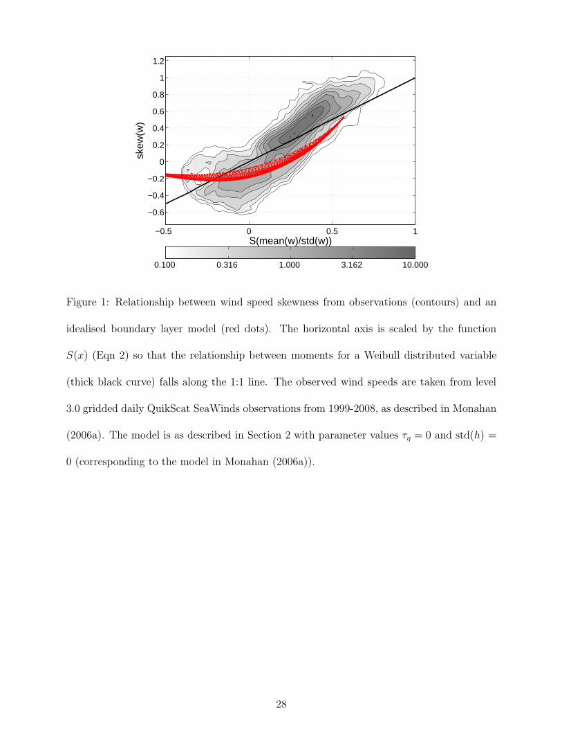
and Γ(x) is the gamma function. A plot of the observed relationship between moments for sea

surface winds (contours) and for a Weibull variable (thick black line) is presented in Figure

1, in which the horizontal axis has been scaled so that the Weibull relationship appears as

a 1:1 line. The observed relationship between moments clusters around the Weibull line,

although with a somewhat steeper slope and pronounced curvature to the lower left. While

it is evident from Figure 1 that the Weibull distribution is a good approximation to the pdf

of sea surface winds, it is worth emphasising that this distribution is an empirical model

without mechanistic basis.

Also plotted in Figure 1 is the relationship between moments as simulated by an idealised

3

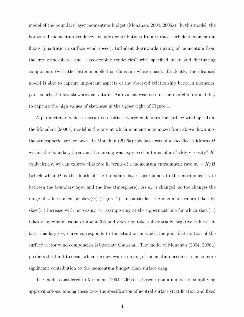
model of the boundary layer momentum budget (Monahan, 2004, 2006a). In this model, the

horizontal momentum tendency includes contributions from surface turbulent momentum

fluxes (quadratic in surface wind speed), turbulent downwards mixing of momentum from

the free atmosphere, and “ageostrophic tendencies” with specified mean and fluctuating

components (with the latter modelled as Gaussian white noise). Evidently, the idealised

model is able to capture important aspects of the observed relationship between moments,

particularly the low-skewness curvature. An evident weakness of the model is its inability

to capture the high values of skewness in the upper right of Figure 1.

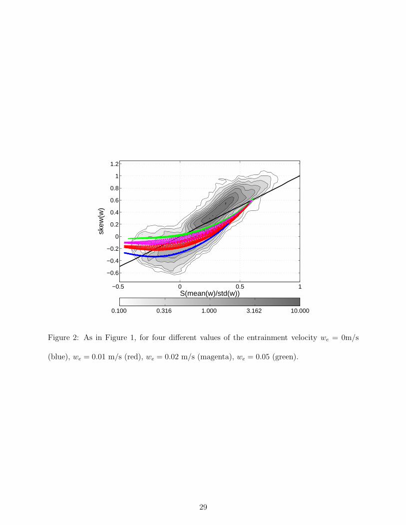
A parameter to which skew(w) is sensitive (where w denotes the surface wind speed) in

the Monahan (2006a) model is the rate at which momentum is mixed from above down into

the atmospheric surface layer. In Monahan (2006a) this layer was of a specified thickness H

within the boundary layer and the mixing was expressed in terms of an ”eddy viscosity” K;

equivalently, we can express this rate in terms of a momentum entrainment rate we = K/H

(which when H is the depth of the boundary layer corresponds to the entrainment rate

between the boundary layer and the free atmosphere). As we is changed, so too changes the

range of values taken by skew(w) (Figure 2). In particular, the maximum values taken by

skew(w) increase with increasing we, asymptoting at the uppermost line for which skew(w)

takes a maximum value of about 0.6 and does not take substantially negative values. In

fact, this large we curve corresponds to the situation in which the joint distribution of the

surface vector wind components is bivariate Gaussian. The model of Monahan (2004, 2006a)

predicts this limit to occur when the downwards mixing of momentum becomes a much more

significant contribution to the momentum budget than surface drag.

The model considered in Monahan (2004, 2006a) is based upon a number of simplifying

approximations; among these were the specification of neutral surface stratification and fixed

4

surface layer thickness. In fact, the boundary-layer momentum budget is influenced by local

surface stratification and boundary layer depth variations in three distinct ways:

1. The surface drag coefficient cd is a function of surface stratification (equivalently -

assuming downgradient fluxes in the surface layer - surface buoyancy fluxes) such that

an unstable stratification enhances surface turbulence (through buoyant generation of

turbulent kinetic energy) and thereby increases surface drag (as the increased turbulent

mixing allows more efficient momentum exchange with the surface). Conversely, stable

stratification suppresses surface turbulence (through buoyant consumption of turbulent

kinetic energy) and decreases surface drag. Monin-Obukhov theory parametrises these

effects through a correction term to the neutral stability drag coefficient that depends

on the Obukhov length L (such that L < 0 for surface heat flux to the atmosphere,

and L > 0 for surface heat flux to the ocean; e.g. Stull, 1997)

2. Deepening of the boundary layer turbulently mixes momentum from the free atmo-

sphere into the boundary layer, inducing a boundary layer momentum tendency. This

turbulent mixing exists even for a boundary layer of constant thickness (the thickness

tendency associated with boundary-layer top turbulent mixing may be balanced or

exceeded by restratifying processes such as radiative cooling to space or large-scale

subsidence, (e.g. Medeiros et al., 2005)), but is stronger when the boundary layer itself

is deepening.

3. In the well-mixed slab boundary layer approximation, momentum tendencies produced

by turbulent momentum fluxes at the surface and the boundary layer top are dis-

tributed across fluid parcels throughout the depth of the boundary layer. As the bound-

ary layer becomes thicker, these interfacial fluxes are therefore diluted and weakened;

5

conversely, as the boundary layer becomes shallower, these fluxes are concentrated and

strengthened. (e.g. Samelson et al., 2006).

Other tendencies driven by horizontal gradients in surface heat fluxes or boundary layer

depth (e.g. mesoscale thermal circulations) are non-local and manifest through the pressure

gradient force. The separation between the influence of surface stratification and boundary

layer depth variations is somewhat artificial, as variations in air-sea temperature difference

play an important role in driving variability in the marine boundary layer thickness (e.g.

Samelson et al., 2006; Small et al., 2008). However, boundary layer thickness variations are

also driven by processes other than surface fluxes, such as those associated by boundary layer

top clouds (e.g. Stevens, 2002; Medeiros et al., 2005). The focus of this study will be on the

direct influence of surface buoyancy fluxes (though modification of the drag coefficient) and

of boundary layer thickness variability (by whatever processes this is generated).

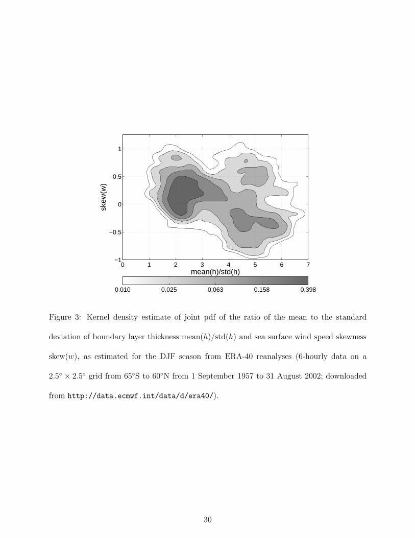
Evidence of a relationship between variability in boundary layer height (denoted h) and

the shape of the wind speed pdf is suggested by the negative correlation between December-

January-February (DJF) 10-m ocean skew(w) and the ratio mean(h)/std(h) (Figure 3), as

determined from the European Centre for Medium Range Weather Forecasts (ECMWF)

ERA-40 reanalysis product (Simmons and Gibson, 2000). It is evident from Figure 3 that in

the ERA-40 reanalysis the wind speed skewness tends to be most positive at locations where

the boundary layer variability is large (relative to the mean boundary layer depth) and the

skewness tends to decrease as variability in h decreases. Of course this anticorrelation is

not perfect, and the representation in the reanalysis data of non-assimilated quantities such

as surface winds and (particularly) boundary layer thickness must be regarded skeptically.

Nevertheless, Figure 3 is derived from a fully complex GCM with a sophisticated boundary

layer scheme. As such, the relationship illustrated in Figure 3 is suggestive that at least

6

one of the missing factors in the idealised boundary layer momentum budget is an active

boundary layer.

The present study generalises the idealised model of the boundary layer momentum

budget developed in Monahan (2004, 2006a) to consider the effects on the pdf of sea surface

winds of surface stratification and variations in boundary layer depth. The generalised

model is still a highly simplified representation of marine boundary layer physics and is

designed to capture the essential qualitative features of the wind speed pdf rather than to

provide a quantitatively precise characterisation. The generalised model of the boundary

layer momentum budget is described in Section 2, followed by a consideration of the effects

of accounting for surface stratification in Section 3. The influence of variability in boundary

layer depth on the pdf of sea surface winds is considered in Section 4, and conclusions follow

in Section 5.

2 Idealised Boundary Layer Momentum Budget Model

The original idealised boundary layer momentum budget of Monahan (2004, 2006a) modelled

surface vector wind tendencies as resulting from an imbalance between four forces: (1) a

mean “non-local” ageostrophic tendency, (2) fluctuations in the “ageostrophic” forcing, (3)

surface drag, and (4) downwards mixing of momentum from above the (fixed-depth) layer.

Because the layer thickness was fixed, the character of the winds above z = H did not need

to be modelled explicitly and the associated tendencies were subsumed into the mean and

fluctuating “ageostrophic” forcing. In the present study, entrainment of momentum from

the free atmosphere is a variable and potentially intermittent process, and is thus modelled

explicitly.

7

Expressing the above ideas quantitatively: the boundary-layer momentum budget is given

by

du

dt=

A︷︸︸︷

U s

τs+

B︷︸︸︷ηu

τs−

C︷ ︸︸ ︷

cd(w, T )

hwu +

D︷ ︸︸ ︷we

h(U(h + δ) − u)+

E︷ ︸︸ ︷

σuW1 (3)

dv

dt=

ηv

τs

− cd(w, T )

hwv +

we

h(V (h + δ) − v) + σuW2. (4)

The “non-local” ageostrophic forcing is expressed as the sum of mean (terms A) and fluc-

tuating (term B) components (by definition there is no component of the mean forcing in

the cross-mean wind direction). The quantity τs is a characteristic surface wind adjustment

timescale, specified so that mean(u) ∼ Us. Fluctuations in large-scale forcing are modelled

as are red-noise processes with autocorrelation timescale τη and mean zero:

d

dtηu = − 1

τηηu +

√

2(τη + τs)σenv

τηW3 (5)

d

dtηv = − 1

τη

ηv +√

2(τη + τs)σenv

τη

W4. (6)

The noise terms are scaled so that σ2env is approximately the contribution to the variance

of u (or v) associated with the non-local ageostrophic forcing (more precisely, a variable z

described by dz/dt = (−z+ηu)/τs has standard deviation σenv). Surface and boundary-layer

top eddy momentum fluxes are given by terms C and D, respectively. Along with large-scale

forcing of the boundary layer momentum budget, local fluctuating forcing is represented

as white-noise forcing with scaling coefficient σu (term E). The random processes Wi are

mutually uncorrelated white noise processes:

mean(Wi(t)Wj(s)) = δ(t − s)δij. (7)

Variability in boundary layer depth is driven by an imbalance in tendencies between

stratifying and mixing processes:

d

dth = − 1

τhh + w∗

e +ξ

τh. (8)

8

The first term in Eqn. (8) represents the average tendency of restratifying processes (e.g.

subsidence, radiation to space) which cause boundary layer heights to decrease on a timescale

τh, while the second term represents a baseline turbulent entrainment velocity which acts

to deepen the mixed layer. Finally, the third term describes the net effect of variability in

restratifying and entrainment rates and is described for simplicity as a red-noise process with

autocorrelation timescale τξ:

d

dtξ = − 1

τξ

ξ +Σξ

τξ

W5 (9)

(where W5 is a white noise process uncorrelated with Wj , j = 1, ..., 4).To ensure that the

boundary layer height does not become negative, h is not allowed to decrease below a mini-

mum value, hmin. To a good approximation (exact in the absence of the lower limit hmin) h

has the stationary standard deviation

std(h) =Σξ

√

2(τh + τξ)(10)

and autocorrelation function

chh(t) =1

τh − τξ

[

τh exp

(

−|t|τh

)

− τξ exp

(

−|t|τξ

)]

. (11)

The rate at which momentum is mixed from the free atmosphere into the boundary layer

is determined by the entrainment velocity

we = w∗e +

1

τh

max (ξ, 0) . (12)

The first of these terms is the constant background entrainment rate, while the second is

associated with those fluctuations in mixed layer depth which tend to deepen the mixed layer

(restratifying processes do not unmix the boundary layer).

Note that as modelled boundary layer variability is not influenced by surface stratifica-

tion, wind speeds, or the state of the free atmosphere. In reality, the turbulent entrainment

9

rate at the top of the marine boundary layer is influenced by a number of factors, includ-

ing the strength of the boundary layer-top inversion, generation of turbulent kinetic energy

within the boundary layer (a process which is influenced by surface buoyancy fluxes) and the

radiatively-driven generation of turbulence within boundary layer-top clouds (e.g. Stevens,

2002). From the point of view of the main concerns of this study, viz. the direct influences

of surface stratification (through the drag coefficient) and boundary layer depth variability

on the pdf of sea surface winds, the fact that the boundary layer depth is variable is more

important than the precise details of why it is variable. Nevertheless, the neglect of feedbacks

of state variables on boundary layer tendencies (other than the simple relaxation term on

h) is a substantial approximation. Surface winds modulate both surface fluxes and the me-

chanical generation of turbulence, and the strength of the boundary layer-top inversion can

be expected to depend on h. A more detailed representation of boundary layer tendencies

including the influence of the winds would involve a substantial increase in the complexity

of the model (involving for example the introduction of new prognostic variables such as

boundary layer potential temperature). The specified boundary layer dynamics represent a

compromise between model simplicity and fidelity to nature motivated by the main concerns

of the present study.

Over a short period of time the boundary layer may deepen, shallow, and deepen again;

if this variability is sufficiently rapid, the second deepening will bring the boundary layer top

into contact with free atmospheric air that retains some memory of earlier contact with the

boundary layer. It is therefore desirable to incorporate into the model a simplified prognostic

representation of the free atmosphere wind profile U(z, t) = (U(z, t), V (z, t)). Within the

boundary layer, U(z, t) and u(t) coincide:

U(z, t) = u(t) 0 < z < h(t), (13)

10

while above z = h(t), in the free atmosphere, the horizontal winds relax on a timescale τr to

the “large-scale” environmental profile with shear Λ = (Λu, Λv)

Uenv(z) = (Uenv(z), Venv(z)) = (Us + Λuz, Vs + Λvz), (14)

so

∂tU(z, t) =1

τr(Uenv(z) − U(z, t)) z ≥ h(t). (15)

The free atmospheric winds that are mixed down into the boundary layer are those at a

small height δ above the top of the boundary layer.

The surface stratification influences the momentum budget directly through changes in

the character of boundary layer turbulence. A natural measure of surface stratification is

the difference T between surface air temperature (SAT) and sea surface temperature (SST)

T = SAT − SST. (16)

Unstable stratification (T < 0) enhances turbulence and increases the rate of turbulent

momentum exchange with the underlying surface, increasing cd. Conversely, stable strati-

fication (T > 0) inhibits surface turbulence and reduces cd. The drag coefficient is also a

function of the sea-surface wind speed w (e.g. Csanady, 2001), as the generation of surface

ocean waves by surface winds increases surface roughness and therefore drag. At moderate

to strong wind speeds over a developed sea, cd is an increasing function of w. For very weak

winds, cd may also increase as w decreases in accordance with the characteristics of drag

over an aerodynamically smooth surface. The functional dependence of cd on T and w in

observations displays considerable scatter (as a result of varying conditions and the difficulty

of measurements), so there is no uniquely agreed-upon functional form for this relationship.

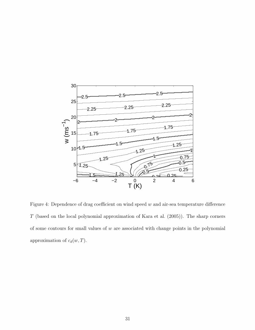
In this study, we will make use of the drag coefficient cd(w, T ) given by a local polynomial

11

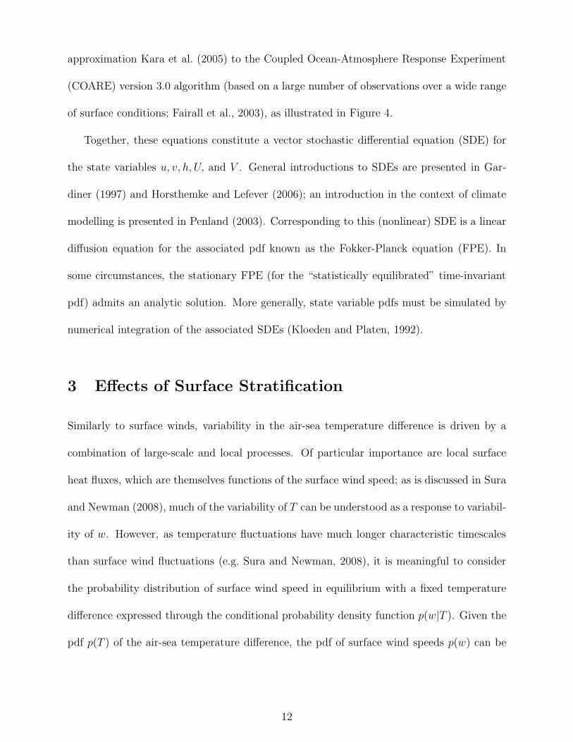
approximation Kara et al. (2005) to the Coupled Ocean-Atmosphere Response Experiment

(COARE) version 3.0 algorithm (based on a large number of observations over a wide range

of surface conditions; Fairall et al., 2003), as illustrated in Figure 4.

Together, these equations constitute a vector stochastic differential equation (SDE) for

the state variables u, v, h, U, and V . General introductions to SDEs are presented in Gar-

diner (1997) and Horsthemke and Lefever (2006); an introduction in the context of climate

modelling is presented in Penland (2003). Corresponding to this (nonlinear) SDE is a linear

diffusion equation for the associated pdf known as the Fokker-Planck equation (FPE). In

some circumstances, the stationary FPE (for the “statistically equilibrated” time-invariant

pdf) admits an analytic solution. More generally, state variable pdfs must be simulated by

numerical integration of the associated SDEs (Kloeden and Platen, 1992).

3 Effects of Surface Stratification

Similarly to surface winds, variability in the air-sea temperature difference is driven by a

combination of large-scale and local processes. Of particular importance are local surface

heat fluxes, which are themselves functions of the surface wind speed; as is discussed in Sura

and Newman (2008), much of the variability of T can be understood as a response to variabil-

ity of w. However, as temperature fluctuations have much longer characteristic timescales

than surface wind fluctuations (e.g. Sura and Newman, 2008), it is meaningful to consider

the probability distribution of surface wind speed in equilibrium with a fixed temperature

difference expressed through the conditional probability density function p(w|T ). Given the

pdf p(T ) of the air-sea temperature difference, the pdf of surface wind speeds p(w) can be

12

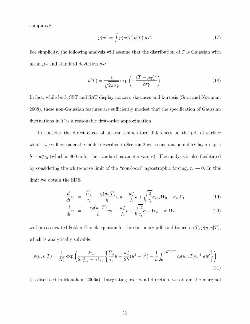
computed:

p(w) =∫

p(w|T )p(T ) dT . (17)

For simplicity, the following analysis will assume that the distribution of T is Gaussian with

mean µT and standard deviation σT :

p(T ) =1

√

2πσ2T

exp

(

−(T − µT )2

2σ2T

)

. (18)

In fact, while both SST and SAT display nonzero skewness and kurtosis (Sura and Newman,

2008), these non-Gaussian features are sufficiently modest that the specification of Gaussian

fluctuations in T is a reasonable first-order approximation.

To consider the direct effect of air-sea temperature differences on the pdf of surface

winds, we will consider the model described in Section 2 with constant boundary layer depth

h = w∗eτh (which is 800 m for the standard parameter values). The analysis is also facilitated

by considering the white-noise limit of the “non-local” ageostrophic forcing, τη → 0. In this

limit we obtain the SDE

d

dtu =

U s

τs− cd(w, T )

hwu − w∗

e

hu +

√

2

τsσenvW3 + σuW1 (19)

d

dtv = −cd(w, T )

hwv − w∗

e

hv +

√

2

τs

σenvW4 + σuW2, (20)

with an associated Fokker-Planck equation for the stationary pdf conditioned on T , p(u, v|T ),

which is analytically solvable:

p(u, v|T ) =1

N1

exp

(

2τs

2σ2env + σ2

uτs

{

U s

τsu − w∗

e

2h(u2 + v2) − 1

h

∫√

u2+v2

0

cd(w′, T )w′2 dw′

})

(21)

(as discussed in Monahan, 2006a). Integrating over wind direction, we obtain the marginal

13

pdf of the wind speed (conditioned on T )

p(w|T ) =1

N2

wI0

(

2Usw

2σ2env + σ2

uτs

)

exp

(

− 2τs

2σ2env + σ2

uτs

{w∗

e

2hw2 +

1

h

∫ w

0

cd(w′, T )w′2 dw′

})

.

(22)

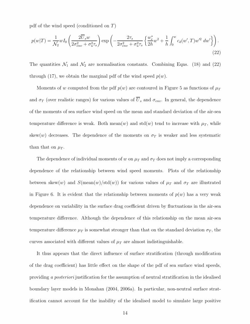
The quantities N1 and N2 are normalisation constants. Combining Eqns. (18) and (22)

through (17), we obtain the marginal pdf of the wind speed p(w).

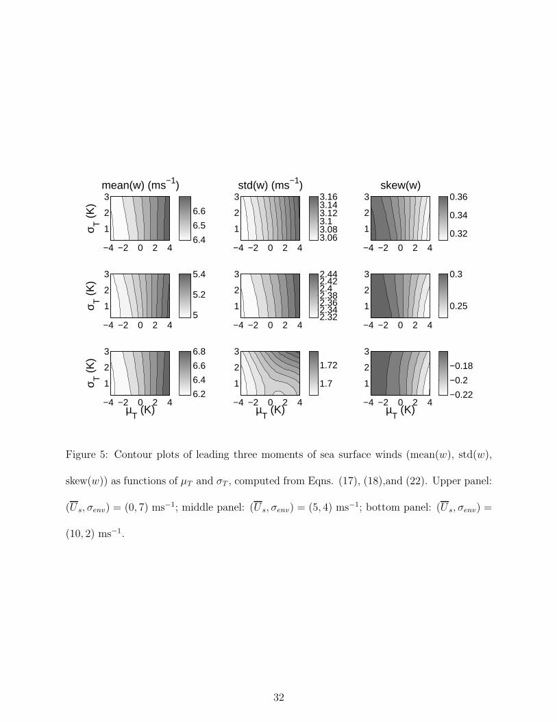
Moments of w computed from the pdf p(w) are contoured in Figure 5 as functions of µT

and σT (over realistic ranges) for various values of U s and σenv. In general, the dependence

of the moments of sea surface wind speed on the mean and standard deviation of the air-sea

temperature difference is weak. Both mean(w) and std(w) tend to increase with µT , while

skew(w) decreases. The dependence of the moments on σT is weaker and less systematic

than that on µT .

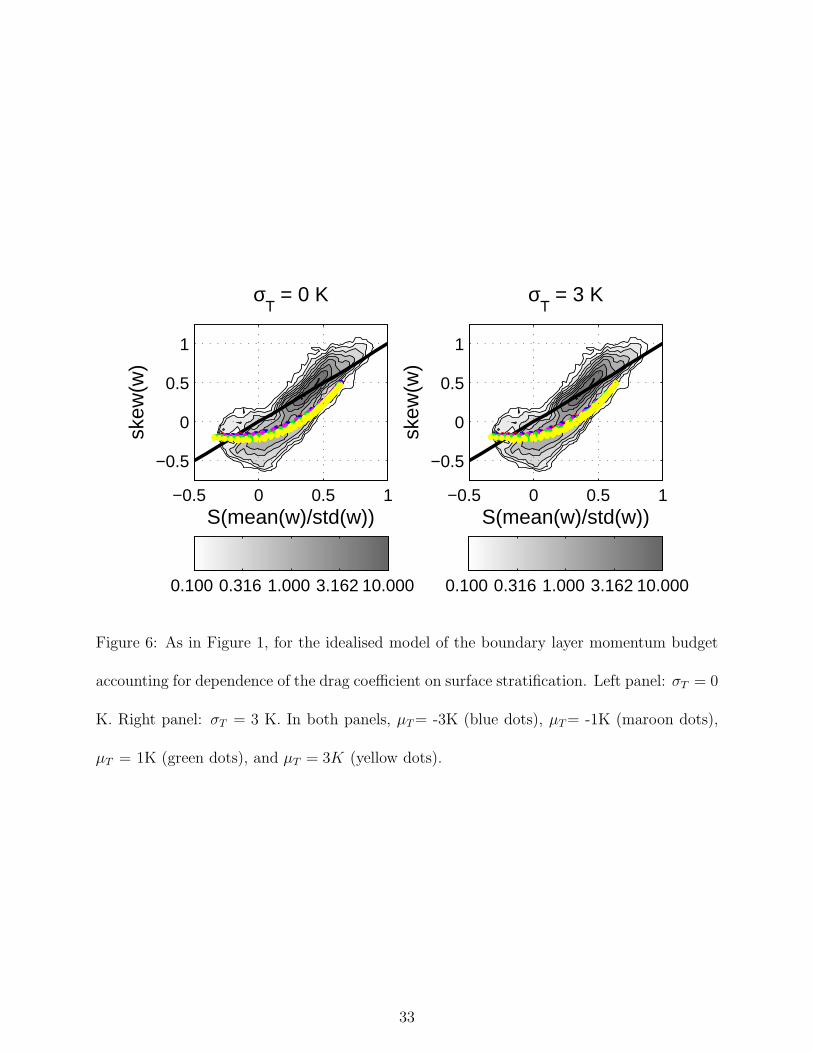
The dependence of individual moments of w on µT and σT does not imply a corresponding

dependence of the relationship between wind speed moments. Plots of the relationship

between skew(w) and S(mean(w)/std(w)) for various values of µT and σT are illustrated

in Figure 6. It is evident that the relationship between moments of p(w) has a very weak

dependence on variability in the surface drag coefficient driven by fluctuations in the air-sea

temperature difference. Although the dependence of this relationship on the mean air-sea

temperature difference µT is somewhat stronger than that on the standard deviation σT , the

curves associated with different values of µT are almost indistinguishable.

It thus appears that the direct influence of surface stratification (through modification

of the drag coefficient) has little effect on the shape of the pdf of sea surface wind speeds,

providing a posteriori justification for the assumption of neutral stratification in the idealised

boundary layer models in Monahan (2004, 2006a). In particular, non-neutral surface strat-

ification cannot account for the inability of the idealised model to simulate large positive

14

wind speed skewness in conditions of light mean winds. He et al. (2009) also find that in

terrestrial areas classified as “open water” (lakes and coastal regions) the diurnal and sea-

sonal evolution of p(w) is much weaker than over open land or forested regions, suggesting a

much weaker influence of surface heat fluxes over water where the momentum and thermal

roughness lengths both tend to be small (Garratt, 1992). Over land, there is evidence that

surface buoyancy fluxes (both mean and variability) have a pronounced influence on the

character of the surface wind speed pdf (He et al., 2009). In the following section, we will

consider the effects of variable boundary layer depth on the shape of p(w).

4 Effects of Variable Boundary Layer Depth

The correlation between wind speed skewness and boundary layer depth variability illustrated

in Figure 3 suggests that the specification of a fixed layer depth in the idealised boundary

layer momentum budget of Monahan (2004, 2006a) may contribute to this model’s inability

to account for the observed large positive values of skew(w) illustrated in Figure 1. To test

this hypothesis, moments of w were computed from the idealised model of the boundary

layer momentum budget described in Section 2 over broad ranges of the parameters U s, σenv,

and std(h). Because the Fokker-Planck equation associated with this model does not admit

analytic solutions (other than in the limit considered in Section 3), these stochastic differ-

ential equations were integrated numerically (for 15 years of model time, with output saved

every six hours) using a standard forward-Euler technique (Kloeden and Platen, 1992). It

was demonstrated in Section 3 that the direct influence of air-sea temperature differences

on the momentum budget is small, so these numerical simulations were carried out with

constant neutral stratification (µT = σT = 0 K).

15

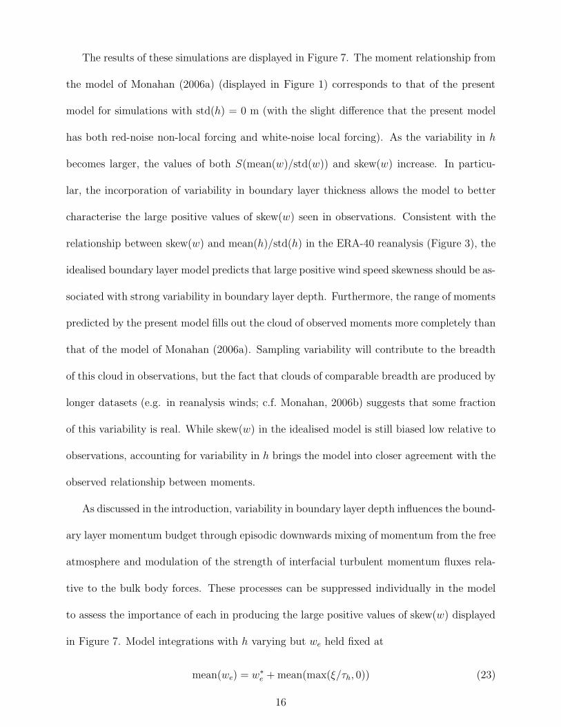
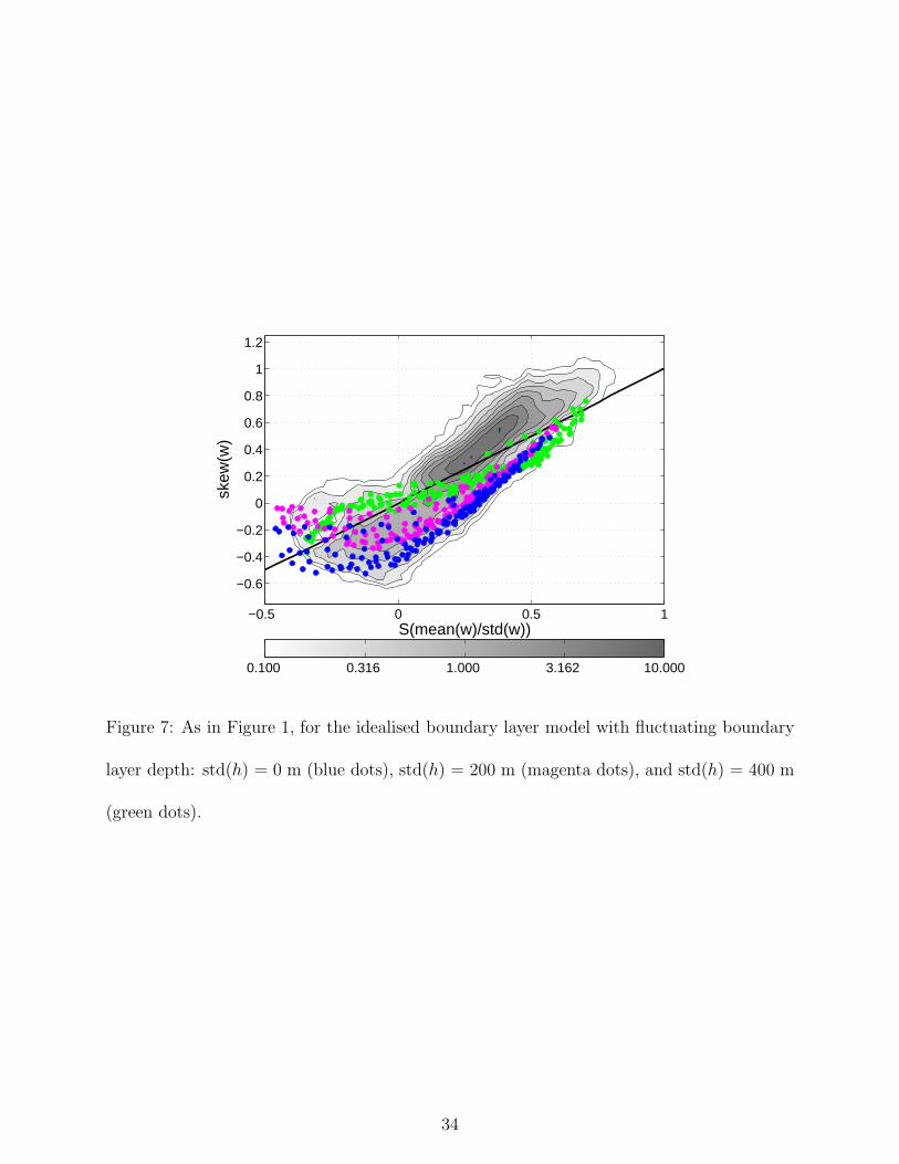
The results of these simulations are displayed in Figure 7. The moment relationship from

the model of Monahan (2006a) (displayed in Figure 1) corresponds to that of the present

model for simulations with std(h) = 0 m (with the slight difference that the present model

has both red-noise non-local forcing and white-noise local forcing). As the variability in h

becomes larger, the values of both S(mean(w)/std(w)) and skew(w) increase. In particu-

lar, the incorporation of variability in boundary layer thickness allows the model to better

characterise the large positive values of skew(w) seen in observations. Consistent with the

relationship between skew(w) and mean(h)/std(h) in the ERA-40 reanalysis (Figure 3), the

idealised boundary layer model predicts that large positive wind speed skewness should be as-

sociated with strong variability in boundary layer depth. Furthermore, the range of moments

predicted by the present model fills out the cloud of observed moments more completely than

that of the model of Monahan (2006a). Sampling variability will contribute to the breadth

of this cloud in observations, but the fact that clouds of comparable breadth are produced by

longer datasets (e.g. in reanalysis winds; c.f. Monahan, 2006b) suggests that some fraction

of this variability is real. While skew(w) in the idealised model is still biased low relative to

observations, accounting for variability in h brings the model into closer agreement with the

observed relationship between moments.

As discussed in the introduction, variability in boundary layer depth influences the bound-

ary layer momentum budget through episodic downwards mixing of momentum from the free

atmosphere and modulation of the strength of interfacial turbulent momentum fluxes rela-

tive to the bulk body forces. These processes can be suppressed individually in the model

to assess the importance of each in producing the large positive values of skew(w) displayed

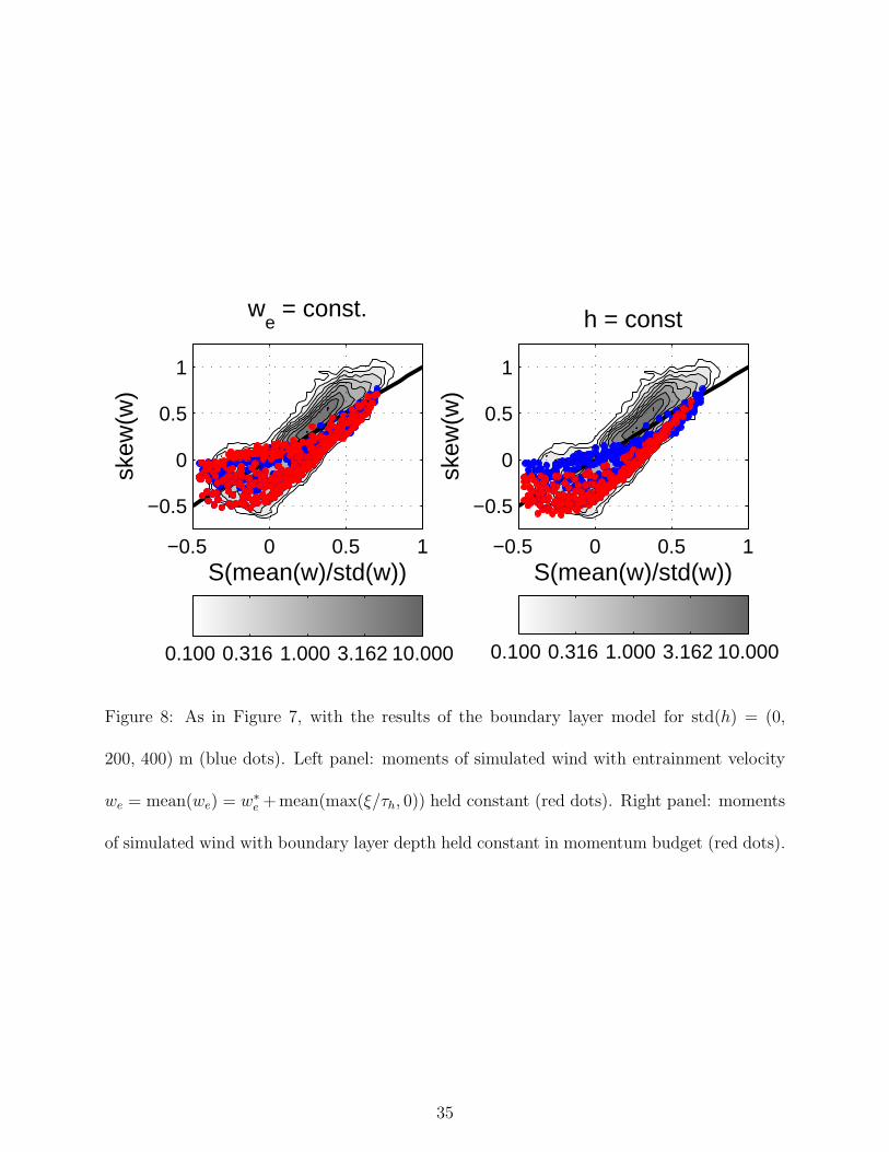
in Figure 7. Model integrations with h varying but we held fixed at

mean(we) = w∗e + mean(max(ξ/τh, 0)) (23)

16

(Figure 8, left panel) demonstrate that the simulated wind speed moments are essentially

unchanged from those of the full model with variable we. In contrast, integrations with we

varying but h held fixed in Eqns. (3) and (4) for the surface vector wind momentum budget

(Figure 8, right panel) demonstrate that in this model the variable downwards mixing of

momentum from aloft is not responsible for producing the larger positive values of skew(w)

produced by the full model. These results are consistent with those of Samelson et al.

(2006), in which the importance to the coupling between wind stress and sea surface tem-

perature of variations in boundary layer depth relative to downwards mixing of momentum

was emphasized.

5 Conclusions

This study has considered the influence of surface stratification and variable boundary layer

thickness on the shape of the probability density function of sea surface wind speeds. As

has been shown in previous studies (e.g. Monahan, 2006a, 2007), the pdf of sea surface

wind speed is characterised by a relationship between the shape of the pdf (as measured by

skewness) and measures of the “size” of the pdf (as measured by the ratio of the mean to the

standard deviation). An earlier mechanistic study of the pdf of sea surface wind speeds using

an idealised model of the boundary layer momentum budget, assuming neutral stratification

and constant boundary layer depth, resulted in a reasonable first order approximation to this

relationship between moments (Monahan, 2006a). However, this earlier model was not able

to account for the large positive wind speed skewnesses seen in observations in conditions

of light and variable winds . A generalisation of this earlier idealised model was used to

assess the relative importance of surface stability-driven variations in the drag coefficient, the

17

downwards mixing of momentum from aloft in a deepening boundary layer, and the dilution

(concentration) of eddy momentum fluxes at the surface and the top of the boundary layer

as the boundary layer deepens (shallows). The following conclusions were obtained.

• While surface stratification (as measured by the air-sea temperature difference) influ-

ences the simulated moments of the surface wind speed pdf, it has an insubstantial

effect on the modelled relationship between surface wind speed moments. In particu-

lar, over a broad (and physically realistic) range of values of the mean and standard

deviation of T = SAT-SST, the model was unable to simulate the large positive wind

speed skewnesses seen in observations.

• Accounting for variability in boundary layer thickness improves the agreement between

the observed and simulated relationships between sea surface wind moments. In partic-

ular, larger positive values of skew(w) are simulated in conditions of weak and variable

winds (small mean(w)/std(w)). These improvements in agreement between simulated

and observed surface moments are due primarily to the dilution/concentration of eddy

momentum fluxes at the surface and the boundary layer top (relative to the body

forces) associated with variations in boundary layer thickness. The episodic down-

wards mixing of momentum from the free atmosphere in the model had little effect on

the relationship between wind speed moments.

The ERA-40 reanalyses are characterised by a relationship between sea surface wind speed

skewness and boundary layer variability, such that skew(w) is a decreasing function of the

ratio mean(h)/std(h). That is, the reanalysis winds are most positively skewed in regions

where variability in boundary layer thickness is relatively large compared to its mean value.

While reanalysis data are not observations, and extreme caution must be exercised in con-

18

sideration of a derived field such as boundary layer height, this relationship indicates that a

complex model containing a broad range of physical processes displays a correlation between

the shape of the wind speed pdf and the (relative) variability of the boundary layer thickness

in broad agreement with that predicted by the idealised model of the present study.

While surface stratification does not appear to have a substantial direct influence (through

the drag coefficient) on the shape of the wind speed pdf over the ocean, the same is not

true over land. He et al. (2009) demonstrate that in open and wooded areas in the North

American domain there is a strong diurnal cycle in the relationship between mean(w)/std(w)

and mean(w), such that for larger values of the ratio the wind speed skewness values are much

smaller during the day than they are at night. Furthermore, this study provided evidence

that these changes in the shape of the land surface wind speed pdf are produced by surface

buoyancy fluxes. In general, thermal roughness lengths are larger over land than over water

(e.g. Garratt, 1992), so it is physically reasonable that surface stratification should exercise

a stronger direct influence on the drag coefficient over land than over water.

While incorporation of variability in boundary layer thickness brings the model simulated

relationship between wind speed moments into closer agreement with the observed relation-

ship, significant model-observation differences remain. In particular, for larger values of the

ratio mean(w)/std(w) the modelled relationship between moments is more similar to that of

the Weibull distribution than that of the observed sea surface winds: values of skew(w) are

still systematically underestimated. Of course, while the present model is more general than

that considered in Monahan (2006a), it remains a highly idealised single-column slab model.

It is possible that the model deficiencies would be addressed through a more complete consid-

eration of vertical and horizontal momentum transport in the boundary layer. Furthermore,

the present model represents as constant in time the profile to which the free atmosphere

19

winds relax; in reality, this profile varies with the large-scale weather. The present study

has also made the simplifying assumption that variability in boundary layer thickness can

be decoupled from variability in surface stratification and from the winds themselves. In

fact, surface buoyancy fluxes are one contributor (among others) to the dynamics of the

boundary layer, and are particularly important in the vicinity of oceanic fronts and eddies

(e.g. Spall, 2007; Small et al., 2008) where SST changes are particularly pronounced. A more

complete model accounting for the influence of various processes driving the boundary layer

top entrainment velocity (including the influence of surface winds) would need to represent

the profiles of (moist) thermodynamic and radiative processes within the boundary layer

(e.g. Stevens, 2002; Medeiros et al., 2005). Such a model would represent a dramatic in-

crease in complexity relative to the model considered in the present study; a more thorough

consideration of the influence of these various boundary layer processes on the pdf of surface

wind speeds is a potentially important direction of future research.

The analysis presented in this study provides further insight regarding the physical factors

that control the shape of the sea surface wind speed pdf. This developing mechanistic

understanding holds the promise of improvements to the estimation of surface fluxes and

surface wind power density from observations, and their simulation in GCMs. Sea surface

winds are a geophysical field of fundamental importance to the coupled climate system; as

we improve our understanding of this field, so our understanding improves of the climate

past, present, and future.

20

Acknowledgements

The author gratefully acknowledges support from the Natural Sciences and Engineering

Research Council of Canada. The author would like to thank Yanping He for valuable

comments on this manuscript.

21

References

Chelton, D. B., M. G. Schlax, M. H. Freilich, and R. F. Milliff, 2004: Satellite measurements

reveal persistent small-scale features in ocean winds. Science, 303, 978–983.

Csanady, G., 2001: Air-Sea Interaction: Laws and Mechanisms. Cambridge University Press,

Cambridge, UK, 248 pp.

Fairall, C. W., E. F. Bradley, J. E. Hare, A. A. Grachev, and J. B. Edson, 2003: Bulk

parameterization of air-sea fluxes: Updates and verification for the COARE algorithm. J.

Climate, 16, 571–591.

Gardiner, C. W., 1997: Handbook of Stochastic Methods for Physics, Chemistry, and the

Natural Sciences. Springer, 442 pp.

Garratt, J., 1992: The Atmospheric Boundary Layer. Cambridge University Press, Cam-

bridge, UK, 316 pp.

He, Y., A. H. Monahan, C. G. Jones, A. Dai, S. Biner, D. Caya, and K. Winger, 2009: Land

surface wind speed probability distributions in North America: Observations, theory, and

regional climate model simulations. J. Geophys. Res., in review.

Horsthemke, W. and R. Lefever, 2006: Noise-Induced Transitions: Theory and Applications

in Physics, Chemistry and Biology. Springer-Verlag, Berlin, 318 pp.

Jet Propulsion Laboratory, 2001: SeaWinds on QuikSCAT Level 3: Daily, Gridded Ocean

Wind Vectors. Tech. Rep. Tech. Rep. JPL PO.DAAC Product 109, California Institute of

Technology.

22

Kara, A. B., H. E. Hurlburt, and A. J. Wallcraft, 2005: Stability-dependent exchange coef-

ficients for air-sea fluxes. J. Atmos. Ocean. Tech., 22, 1080–1094.

Kloeden, P. E. and E. Platen, 1992: Numerical Solution of Stochastic Differential Equations.

Springer-Verlag, Berlin, 632 pp.

Mahrt, L. and J. Sun, 1995: The subgrid velocity scale in the bulk aerodynamic relationship

for spatially averaged scalar fluxes. Mon. Weath. Rev., 123, 3032–3041.

Medeiros, B., A. Hall, and B. Stevens, 2005: What controls the mean depth of the PBL? J.

Climate, 18, 3157–3172.

Monahan, A. H., 2004: A simple model for the skewness of global sea-surface winds. J.

Atmos. Sci., 61, 2037–2049.

Monahan, A. H., 2006a: The probability distribution of sea surface wind speeds. Part I:

Theory and SeaWinds observations. J. Climate, 19, 497–520.

Monahan, A. H., 2006b: The probability distribution of sea surface wind speeds. Part II:

Dataset intercomparison and seasonal variability. J. Climate, 19, 521–534.

Monahan, A. H., 2007: Empirical models of the probability distribution of sea surface wind

speeds. J. Climate, 20, 5798–5814.

Penland, C., 2003: Noise out of chaos and why it won’t go away. Bull. Am. Met. Soc., 84,

921–925.

Samelson, R., E. Skyllingstad, D. Chelton, S. Esbensen, L. O’Neill, and N. Thum, 2006: On

the coupling of wind stress and sea surface temperature. J. Climate, 19, 1557–1566.

23

Simmons, A. and J. Gibson, 2000: The ERA-40 Project Plan. ERA-40 Project Report Series

No. 1, ECMWF, Reading, RG2 9AX, UK. 63 pp.

Small, R., et al., 2008: Air-sea interaction over ocean fronts and eddies. Dyn. Atmos. Oceans,

45, 274–319.

Spall, M. A., 2007: Midlatitude wind stress - sea surface temperature coupling in the vicinity

of oceanic fronts. J. Climate, 20, 3785–3801.

Stevens, B., 2002: Entrainment in stratocumulus-topped mixed layers. Q. J. R. Meteorol.

Soc., 128, 2663–2690.

Stull, R. B., 1997: An Introduction to Boundary Layer Meteorology. Kluwer, Dordrecht, 670

pp.

Sura, P. and M. Newman, 2008: The impact of rapid wind variability upon air-sea thermal

coupling. J. Climate, 21, 621–637.

Wanninkhof, R., S. C. Doney, T. Takahashi, and W. R. McGillis, 2002: The effect of us-

ing time-averaged winds on regional air-sea CO2 fluxes. Gas Transfer at Water Surfaces,

M. A. Donelan, W. M. Drennan, E. S. Saltzman, and R. Wanninkhof, Eds., American

Geophysical Union, 351–356.

24

Figure Captions

Figure 1: Relationship between wind speed skewness from observations (contours) and an

idealised boundary layer model (red dots). The horizontal axis is scaled by the function

S(x) (Eqn 2) so that the relationship between moments for a Weibull distributed variable

(thick black curve) falls along the 1:1 line. The observed wind speeds are taken from level

3.0 gridded daily QuikScat SeaWinds observations from 1999-2008, as described in

Monahan (2006a). The model is as described in Section 2 with parameter values τη = 0

and std(h) = 0 (corresponding to the model in Monahan (2006a)).

Figure 2: As in Figure 1, for four different values of the entrainment velocity we = 0m/s

(blue), we = 0.01 m/s (red), we = 0.02 m/s (magenta), we = 0.05 (green).

Figure 3: Kernel density estimate of joint pdf of the ratio of the mean to the standard

deviation of boundary layer thickness mean(h)/std(h) and sea surface wind speed skewness

skew(w), as estimated for the DJF season from ERA-40 reanalyses (6-hourly data on a

2.5◦ × 2.5◦ grid from 65◦S to 60◦N from 1 September 1957 to 31 August 2002; downloaded

from http://data.ecmwf.int/data/d/era40/).

Figure 4: Dependence of drag coefficient on wind speed w and air-sea temperature

difference T (based on the local polynomial approximation of Kara et al. (2005)). The

sharp corners of some contours for small values of w are associated with change points in

the polynomial approximation of cd(w, T ).

Figure 5: Contour plots of leading three moments of sea surface winds (mean(w), std(w),

skew(w)) as functions of µT and σT , computed from Eqns. (17), (18),and (22). Upper

panel: (U s, σenv) = (0, 7) ms−1; middle panel: (U s, σenv) = (5, 4) ms−1; bottom panel:

(U s, σenv) = (10, 2) ms−1.

25

Figure 6: As in Figure 1, for the idealised model of the boundary layer momentum budget

accounting for dependence of the drag coefficient on surface stratification. Left panel:

σT = 0 K. Right panel: σT = 3 K. In both panels, µT = -3K (blue dots), µT = -1K (maroon

dots), µT = 1K (green dots), and µT = 3K (yellow dots).

Figure 7: As in Figure 1, for the idealised boundary layer model with fluctuating

boundary layer depth: std(h) = 0 m (blue dots), std(h) = 200 m (magenta dots), and

std(h) = 400 m (green dots).

Figure 8: As in Figure 7, with the results of the boundary layer model for std(h) = (0,

200, 400) m (blue dots). Left panel: moments of simulated wind with entrainment velocity

we = mean(we) = w∗e + mean(max(ξ/τh, 0)) held constant (red dots). Right panel:

moments of simulated wind with boundary layer depth held constant in momentum budget

(red dots).

26

Table Captions

Table 1: Model coordinates and state variables.

Table 2: Model parameters and standard values.

27

S(mean(w)/std(w))

skew

(w)

−0.5 0 0.5 1

−0.6

−0.4

−0.2

0

0.2

0.4

0.6

0.8

1

1.2

0.100 0.316 1.000 3.162 10.000

Figure 1: Relationship between wind speed skewness from observations (contours) and an

idealised boundary layer model (red dots). The horizontal axis is scaled by the function

S(x) (Eqn 2) so that the relationship between moments for a Weibull distributed variable

(thick black curve) falls along the 1:1 line. The observed wind speeds are taken from level

3.0 gridded daily QuikScat SeaWinds observations from 1999-2008, as described in Monahan

(2006a). The model is as described in Section 2 with parameter values τη = 0 and std(h) =

0 (corresponding to the model in Monahan (2006a)).

28

S(mean(w)/std(w))

skew

(w)

−0.5 0 0.5 1

−0.6

−0.4

−0.2

0

0.2

0.4

0.6

0.8

1

1.2

0.100 0.316 1.000 3.162 10.000

Figure 2: As in Figure 1, for four different values of the entrainment velocity we = 0m/s

(blue), we = 0.01 m/s (red), we = 0.02 m/s (magenta), we = 0.05 (green).

29

mean(h)/std(h)

skew

(w)

0 1 2 3 4 5 6 7−1

−0.5

0

0.5

1

0.010 0.025 0.063 0.158 0.398

Figure 3: Kernel density estimate of joint pdf of the ratio of the mean to the standard

deviation of boundary layer thickness mean(h)/std(h) and sea surface wind speed skewness

skew(w), as estimated for the DJF season from ERA-40 reanalyses (6-hourly data on a

2.5◦ × 2.5◦ grid from 65◦S to 60◦N from 1 September 1957 to 31 August 2002; downloaded

from http://data.ecmwf.int/data/d/era40/).

30

0.25 0.250.250.750.75

1.25

1.251.25

1.251.25

1.75 1.751.75

2.25 2.25 2.25

0.5

0.5

1

11

1.5

1.51.5

1.5

2 2 2 2

2.5 2.5 2.5

T (K)

w (

ms−

1 )

−6 −4 −2 0 2 4 6

5

10

15

20

25

30

Figure 4: Dependence of drag coefficient on wind speed w and air-sea temperature difference

T (based on the local polynomial approximation of Kara et al. (2005)). The sharp corners

of some contours for small values of w are associated with change points in the polynomial

approximation of cd(w, T ).

31

σ T (

K)

mean(w) (ms−1)

−4 −2 0 2 4

1

2

3

6.4

6.5

6.6

std(w) (ms−1)

−4 −2 0 2 4

1

2

3

3.063.083.13.123.143.16

skew(w)

−4 −2 0 2 4

1

2

3

0.32

0.34

0.36

σ T (

K)

−4 −2 0 2 4

1

2

3

5

5.2

5.4

−4 −2 0 2 4

1

2

3

2.322.342.362.382.42.422.44

−4 −2 0 2 4

1

2

3

0.25

0.3

µT (K)

σ T (

K)

−4 −2 0 2 4

1

2

3

6.2

6.4

6.6

6.8

µT (K)

−4 −2 0 2 4

1

2

3

1.7

1.72

µT (K)

−4 −2 0 2 4

1

2

3

−0.22

−0.2

−0.18

Figure 5: Contour plots of leading three moments of sea surface winds (mean(w), std(w),

skew(w)) as functions of µT and σT , computed from Eqns. (17), (18),and (22). Upper panel:

(U s, σenv) = (0, 7) ms−1; middle panel: (U s, σenv) = (5, 4) ms−1; bottom panel: (U s, σenv) =

(10, 2) ms−1.

32

S(mean(w)/std(w))

skew

(w)

σT = 0 K

−0.5 0 0.5 1

−0.5

0

0.5

1

0.100 0.316 1.000 3.162 10.000

S(mean(w)/std(w))

skew

(w)

σT = 3 K

−0.5 0 0.5 1

−0.5

0

0.5

1

0.100 0.316 1.000 3.162 10.000

Figure 6: As in Figure 1, for the idealised model of the boundary layer momentum budget

accounting for dependence of the drag coefficient on surface stratification. Left panel: σT = 0

K. Right panel: σT = 3 K. In both panels, µT = -3K (blue dots), µT = -1K (maroon dots),

µT = 1K (green dots), and µT = 3K (yellow dots).

33

S(mean(w)/std(w))

skew

(w)

−0.5 0 0.5 1

−0.6

−0.4

−0.2

0

0.2

0.4

0.6

0.8

1

1.2

0.100 0.316 1.000 3.162 10.000

Figure 7: As in Figure 1, for the idealised boundary layer model with fluctuating boundary

layer depth: std(h) = 0 m (blue dots), std(h) = 200 m (magenta dots), and std(h) = 400 m

(green dots).

34

S(mean(w)/std(w))

skew

(w)

we = const.

−0.5 0 0.5 1

−0.5

0

0.5

1

0.100 0.316 1.000 3.162 10.000

S(mean(w)/std(w))

skew

(w)

h = const

−0.5 0 0.5 1

−0.5

0

0.5

1

0.100 0.316 1.000 3.162 10.000

Figure 8: As in Figure 7, with the results of the boundary layer model for std(h) = (0,

200, 400) m (blue dots). Left panel: moments of simulated wind with entrainment velocity

we = mean(we) = w∗e +mean(max(ξ/τh, 0)) held constant (red dots). Right panel: moments

of simulated wind with boundary layer depth held constant in momentum budget (red dots).

35

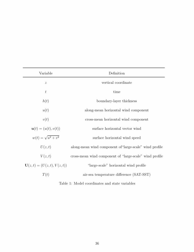
Variable Definition

z vertical coordinate

t time

h(t) boundary-layer thickness

u(t) along-mean horizontal wind component

v(t) cross-mean horizontal wind component

u(t) = (u(t), v(t)) surface horizontal vector wind

w(t) =√

u2 + v2 surface horizontal wind speed

U(z, t) along-mean wind component of“large-scale” wind profile

V (z, t) cross-mean wind component of “large-scale” wind profile

U(z, t) = (U(z, t), V (z, t)) “large-scale” horizontal wind profile

T (t) air-sea temperature difference (SAT-SST)

Table 1: Model coordinates and state variables

36

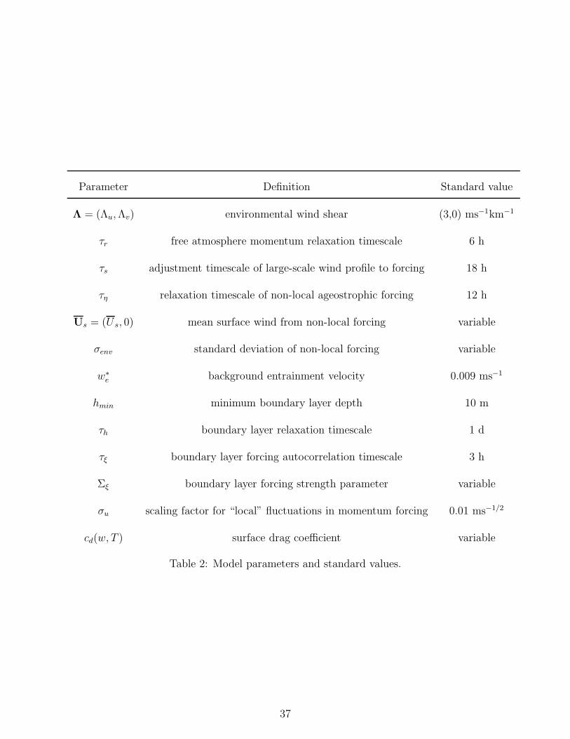
Parameter Definition Standard value

Λ = (Λu, Λv) environmental wind shear (3,0) ms−1km−1

τr free atmosphere momentum relaxation timescale 6 h

τs adjustment timescale of large-scale wind profile to forcing 18 h

τη relaxation timescale of non-local ageostrophic forcing 12 h

Us = (U s, 0) mean surface wind from non-local forcing variable

σenv standard deviation of non-local forcing variable

w∗e background entrainment velocity 0.009 ms−1

hmin minimum boundary layer depth 10 m

τh boundary layer relaxation timescale 1 d

τξ boundary layer forcing autocorrelation timescale 3 h

Σξ boundary layer forcing strength parameter variable

σu scaling factor for “local” fluctuations in momentum forcing 0.01 ms−1/2

cd(w, T ) surface drag coefficient variable

Table 2: Model parameters and standard values.

37