Energy Policy 55 (2013) 117–127

Contents lists available at SciVerse ScienceDirect

Energy Policy

0301-42

http://d

$We

at Stanf

and tw

compet

n Corr

E-m

myorsto1 Se

newly i

journal homepage: www.elsevier.com/locate/enpol

The prospects for cost competitive solar PV power$

Stefan Reichelstein a,n, Michael Yorston b

a Graduate School of Business, Stanford University, USAb Department of MS&E, Stanford University, USA

H I G H L I G H T S

c Assessment of the cost competitiveness of new solar Photovoltaic (PV) installations.c Utility-scale PV installations are not yet cost competitive with fossil fuel power plants.c Commercial-scale installations have already attained cost parity in certain parts of the U.S.c Utility-scale solar PV facilities are on track to become cost competitive by the end of this decade.

a r t i c l e i n f o

Article history:

Received 18 May 2012

Accepted 1 November 2012Available online 25 December 2012

Keywords:

Solar power

Levelized cost of electricity

Public subsidies

15/$ - see front matter & 2012 Elsevier Ltd. A

x.doi.org/10.1016/j.enpol.2012.11.003

would like to acknowledge helpful suggestio

ord University as well as Matthew Campbel

o anonymous reviewers. We are also grate

ent research assistance.

esponding author.

ail addresses: reichelstein@stanford.edu (S. Re

n@stanford.edu (M. Yorston).

e, for instance, the 2011 BP Statistical Review

nstalled capacity of solar PV is estimated to b

a b s t r a c t

New solar Photovoltaic (PV) installations have grown globally at a rapid pace in recent years.

We provide a comprehensive assessment of the cost competitiveness of this electric power source.

Based on data available for the second half of 2011, we conclude that utility-scale PV installations are

not yet cost competitive with fossil fuel power plants. In contrast, commercial-scale installations have

already attained cost parity in the sense that the generating cost of power from solar PV is comparable

to the retail electricity prices that commercial users pay, at least in certain parts of the U.S. This

conclusion is shown to depend crucially on both the current federal tax subsidies for solar power and

an ideal geographic location for the solar installation. Projecting recent industry trends into the future,

we estimate that utility-scale solar PV facilities are on track to become cost competitive by the end of

this decade. Furthermore, commercial-scale installations could reach ‘‘grid parity’’ in about ten years, if

the current federal tax incentives for solar power were to expire at that point.

& 2012 Elsevier Ltd. All rights reserved.

1. Introduction

New installations of solar photovoltaic power have experi-enced rapid growth in recent years. In 2010 alone, almost 17 GWof new photovoltaic (PV) power was installed worldwide. Thisaddition not only represented a 250% increase relative to 2009, itwas also roughly equal to the total cumulative amount of solar PVpower installed since the commercial inception of solar PVtechnology in the 1970s.1 While the impressive growth rates fornew solar energy deployments are uncontroversial, there isconsiderable disagreement regarding the economic fundamentals

ll rights reserved.

ns from seminar participants

l, Roger Noel, Michael Wara

ful to Moritz Hiemann for

ichelstein),

of World Energy. For 2011,

e near 29 GW.

of this energy source. In particular, there appears to be noconsensus as to whether solar PV power is approaching grid

parity, which would require the cost of solar photovoltaic gener-ated electricity to be on par with that generated from otherenergy sources, including fossil fuels such as natural gas or coal.

Proponents of solar power see the rapid growth of the solar PVindustry and the dramatic drop in the price of panels as evidenceof increasing competitiveness of this energy source. In contrast,skeptics attribute the rapid rise of solar PV power primarily togenerous public policies in the form of tax subsidies and directmandates for renewable energy. Furthermore, this camp in thepublic debate argues that the precipitous decline in solar panelprices is not a reflection of favorable economic fundamentals, butrather reflects distress pricing caused by massive new entries intothe solar panel manufacturing industry. As further evidence oflacking economic fundamentals, the skeptics point out that theequity market value of virtually all solar panel manufacturers hasimploded in recent years.

This paper provides an assessment of the cost competitivenessof electricity generated by solar power. We first base this assess-ment on the most recently available data. In light of the dramatic

S. Reichelstein, M. Yorston / Energy Policy 55 (2013) 117–127118

price reductions that solar PV panels have experienced in recentyears, we also seek to extrapolate the prospects for further costreductions that could be obtained with currently available tech-nology. This part of our analysis speaks to the question of whethera continuation of the significant learning-by-doing process thathas characterized this industry is likely to result in ‘grid parity’in the foreseeable future without the need for a technologicalbreakthrough. Our analysis also examines the sensitivity of ourcost assessment to several crucial input variables, such as panelprices, geographic location of the facility and public subsidies inthe form of preferential tax treatment.

The central cost concept in this paper is the Levelized Cost of

Electricity (LCOE). It represents a life cycle cost per kilowatt hour(kWh) and is to be interpreted as the minimum price per kWhthat an electricity generating plant would have to obtain in orderto break-even on its investment over the entire life cycle of thefacility. This break-even calculation essentially amounts to adiscounted cash flow analysis so as to solve for the minimumoutput price required to obtain a net-present value of zero.Unfortunately, the method used for calculating the LCOE in theliterature is far from uniform. We discuss this aspect in moredetail in Section 2 below and in Appendix A2.2

With regard to PV technology platforms, our analysis coversboth the more established crystalline silicon and so-called thin-film solar cells. Crystalline silicon cells are known to be moreefficient in terms of the potential energy converted to electricity.Yet, efficiency of the cell is not a criterion per se in our costanalysis as differences in efficiency are subsumed in both inputcost and electricity output figures. In terms of the scale ofelectricity generation, we consider both utility-scale installations(commonly defined as those larger than 1 MW) and installationsof commercial scale (in a range of 0.1 to 1 MW). The latterinstallations would typically be mounted on large rooftops ofoffice buildings and warehouses. While smaller commercial-scaleinstallations cannot attain the full scale economies of utility-scaleprojects, the benchmark of grid parity is also more lenient to theextent that the applicable cost needs to be compared with retailelectricity prices for commercial users rather than wholesaleprices at the utility-scale level.

Our point estimates for the Levelized Cost of solar PV elec-tricity are based on favorable, albeit realistic scenarios. In parti-cular, we assume that the electricity generating entity canprocure solar panels and other equipment components at thelowest transaction prices observed in the market in late 2011.We also assume that the investor in the solar PV project canbenefit from the federal incentives available for these types ofprojects in the United States—namely a 30% investment tax creditand an accelerated depreciation schedule. Furthermore the loca-tion of the facility is assumed to be an ideal one, for instance, inthe southwestern United States. The favorability of a location isdefined both in terms of insolation and systems degradation, thatis, the decay over time in the electricity output of a solar cell.

We find that that crystalline silicon enjoys a slight cost advan-tage over thin-film, though the two appear generally neck-and-neck for all the scenarios we consider. At around 8 cents per kWh,we find that the LCOE of utility-scale installations is currently notcost competitive with electricity generation from fossil fuels, inparticular from natural gas plants. In contrast, at around 12 centsper kWh, commercial-scale installations appear to have reached

2 Our interpretation of cost competitiveness is that for the party investing in a

solar PV facility the levelized cost per kWh, after inclusion of all tax benefits, does

not exceed the applicable grid price. The latter varies depending on whether the

investing party seeks to sell the electricity output to a distributor at wholesale

prices, or whether it seeks to avoid the retail price of electricity that it would have

pay for its own consumption.

grid parity, at least in locations like Southern California that areboth geographically favorable for solar installations and subject tohigh retail electricity prices. Given that this appears to be themost favorable scenario for solar PV, we use it as the referencecase for further comparisons throughout the paper.

The conclusions we obtain for utility-scale projects suggeststhat the recent growth in such installations is in large part aconsequence of additional public subsidies or governmentmandates for renewable energy. The Renewable Portfolio Standardin California represent such a mandate, while countries likeGermany rely on ‘feed-in-tariffs’ which oblige grid operators tobuy solar electricity at pre-specified prices.3

Our conclusion of grid parity for commercial-scale solar PV isshown to be highly dependent on several crucial assumptions.First, absent the current tax subsidies under the EconomicStabilization Act of 2008, our LCOE estimate would increase byover 75%. Secondly, if the power generating facility were to belocated in New Jersey rather than Southern California, theapplicable LCOE estimate would increase by about 25%. Third,the dramatic recent drop in solar panel prices, in particular the40% drop in 2011 alone, is likely to be a temporary artifact causedby excess production capacity in the solar PV panel industry.Based on the observed long-term price trend for PV modules, weform an estimate of ‘sustainable’ panel prices. We estimate thatif solar panel prices were priced today at the levels suggestedby their long-term price trend, our LCOE figures would increaseby about 12–15%.

In examining the sensitivity of our cost estimates to thesefactors, it should be noted that collectively these factors have a‘super-modular’ effect on the resulting cost estimate. To witness,for a facility based in New Jersey that would have to acquirePV modules at sustainable prices and whose tax treatment isidentical to those of fossil fuel electricity generating plants, theestimated LCOE would increase by about 150% relative to ourbaseline reading of 12 cents per kWh.

Since its inception in the 1970s, prices of solar panels havefallen at a rate that is remarkably consistent with the traditional80% learning-by-doing curve. As documented by Swanson (2006,2011) the market prices for solar panels have on average declinedby approximately 20% every time the cumulative volume of solarPV power installations has doubled. Swanson provides evidencethat a range of variables related to thinner silicon wafers, highersemiconductor yields, improvements in the efficiency of the solarcell and other manufacturing process improvements have allcontributed to substantial and sustained cost reductions. Thesereductions in cost have, in turn, translated into correspondingprice reductions.

If one postulates the continuation of the established learningcurve for photovoltaic modules in the future, it is natural to askhow long it would take current technology—continuously opti-mized over time—to become fully cost competitive. In makingthis projection, we assume that in the future crystalline siliconmodules will indeed be able to maintain the 80% learning factorthey have experienced consistently over the past 30 years. Yet,this pace of learning appears too optimistic for so-called Balance-of-Systems (BoS) components related to cabling, wiring, racking,and permitting. For these BoS costs, which presently account formore than half of the total systems price of new solar installa-tions, we hypothesize a constant percentage reduction each yearrather than the exponential learning curve applicable to modules.

3 The Renewable Portfolio Standard in California commits the state to a quota

of generating at least 33% of all electricity from renewable energy sources by the

year 2020.

S. Reichelstein, M. Yorston / Energy Policy 55 (2013) 117–127 119

Our projections suggest that solar PV will also become costcompetitive for utility-scale facilities by the end of this decade.Furthermore, commercial-scale installation will be able to gen-erate electricity at cost levels that are competitive with currentretail electricity prices within the next ten years, even if thecurrent preferential treatment in the tax code were to expire.From a policy perspective, our analysis therefore suggests thata continuation of the ‘‘continuous growth’’ that the solar PVindustry has experienced since its inception should be sufficient.Put differently, even without any ‘technological breakthrough’,solar PV power should to become economically viable within adecade provided the industry ‘stays the course’.

One caveat of our levelized cost calculations is that they do notreflect two important features of solar PV power: intermittencyand time-of-day peak load patterns. It is well recognized that theintermittency of solar power is one of the principal obstacles forthis source of electricity generation to serve base-load needs,unless it can be combined with some energy storage device.On the other hand, solar PV installations generate a substantialportion of their daily power in the afternoon at hours whenelectricity demand from the grid tends to be relatively high, inparticular in locations where air conditioners account for asubstantial share of the daily electricity consumption. Our costcalculations make no attempt to quantify the economic value, ordiscount, associated with these countervailing features of solar PVpower.4

The remainder of this paper is organized as follows. Section 2presents the details of the LCOE methodology. This section alsohighlights how our implementation of this lifecycle cost conceptdiffers from that in other studies. Section 3 presents our basicpoint estimates for the levelized cost of solar PV. In that sectionwe also examine the robustness of our cost estimates to varia-tions in the most crucial input parameters. Future cost reductionsthat are likely to be obtained if current solar PV technologiesmaintain their past ability for learning-by-doing, are analyzed inSection 4. We conclude in Section 5. Throughout, our calculationsare obtained via an Excel spreadsheet which is available onlineand referred to as the Solar-LCOE Calculator (Reichelstein andYorston, 2012).

5 See, for instance, Ross et al. (2005).6 Our analysis ignores inflation. In an inflationary environment the LCOE

would compound at the rate of inflation. Yet, provided that all production inputs

are subject to the same, constant inflation rate, and this rate is also reflected in the

nominal discount rate, the resulting (initial) LCOE will be unchanged. Thus our

concept of the levelized cost is to be interpreted as a real, rather than a nominal

2. The levelized cost of electricity concept

The Levelized Cost of Electricity (LCOE) is a life-cycle costconcept which seeks to account for all physical assets andresources required to deliver one unit of electricity output.Fundamentally, the LCOE is a break-even value that a powerproducer would need to obtain per Kilowatt-hour (kWh) as salesrevenue in order to justify an investment in a particular powergeneration facility. The 2007-MIT study on ‘‘The Future of Coal’’elaborates on this break-even interpretation of the LCOE with thefollowing verbal definition: ‘‘the levelized cost of electricity is the

constant dollar electricity price that would be required over the life of

the plant to cover all operating expenses, payment of debt and

accrued interest on initial project expenses, and the payment of an

acceptable return to investors’’.The preceding definition makes clear that LCOE is a break-even

figure that must be compatible with present value considerationsfor investors and creditors. Despite widespread references to theLCOE concept, the energy literature does not seem to make use ofa common formula for calculating this average cost. For instance,the MIT study operationalizes the capacity related component of

4 See Borenstein (2012) and Joskow (2011) for further discussion of the

intermittency and peak-load premium aspects of solar power.

the levelized cost of electricity by simply ‘‘applying a 15% carrying

charge to the total plant cost’’. A number of working papers andunpublished reports develop their own version of the LCOEconcept, for instance, Short et al. (1995); Kammen and Pacca,2004, Campbell (2008, 2011); Kolstad and Young (2010).A common approach is to define LCOE as the ratio of ‘‘lifetimecost’’ to ‘‘lifetime electricity generated’’ by the facility. Below, weexamine the consistency of this approach with our formulation.

Consider a single investment in a new power generatingfacility. To assess the life cycle cost of producing electric powerat this facility, we aggregate the upfront capacity investment, thesequence of electricity outputs generated by the facility over itsuseful life, the periodic operating costs required to deliver theelectricity output in each period and any tax related cash flowsthat apply to this type of facility.

Since the LCOE formula yields an output price which leadsequity investors to break-even, it is essential to specify theappropriate discount rate. A standard result in corporate financeis that if the project in question keeps the firm0s leverage ratio(debt over total assets) constant, then the appropriate discountrate is the Weighted Average Cost of Capital (WACC).5 In refer-ence to the above quote in the MIT study, equity holders willreceive ‘‘an acceptable return’’ and debt holders will receive‘‘accrued interest on initial project expenses’’ provided the projectachieves a zero Net-Present Value (NPV) when evaluated at theWACC. We denote this interest rate by r and denote the corre-sponding discount factor by g�1/(1þr).6

For a simplified representation of the LCOE of a new powergenerating facility, suppose initially that there are no periodicoperating costs and no corporate income taxes. The LCOE formulais then based on the following variables:

�

out

ana

of x

T: the useful life of the power generating facility (in years)

� SP: the acquisition cost of capacity (in $/kW) � xt: system degradation factor: the percentage of initial capa-

city that is still functional in year t.

We abstract from any quantity discounts and scale economiesthat in practice can be obtained if the installed capacity reaches acertain threshold size. Thus, there will be no loss generality innormalizing the investment in power capacity to 1 kW. For solarphotovoltaic installations, prices are commonly quoted as ‘‘dollarsper peak Watt DC’’ (abbreviated as $ per Wp).

The system degradation factor, xt , refers to the possibility thatsome output generating capacity may be lost over time.In particular with solar photovoltaic cells it has been observedthat their efficiency diminishes over time. The correspondingdecay is usually represented as a constant percentage factorwhich varies with the particular PV technology and the locationof the installation.7

The power generating facility is theoretically available for8760¼365U24 h, but due to technological, environmental andeconomic constraints, practical capacity is only a percentage ofthe theoretical capacity. This percentage is usually referred to asthe capacity factor, CF. We define the cost of capacity for one

put price.7 In contrast, for other renewable energy sources, for instance, biofuels,

lysts typically anticipate yield improvements which would result in a sequence

t that is increasing over time. See, for instance, NREL (2009).

S. Reichelstein, M. Yorston / Energy Policy 55 (2013) 117–127120

kilowatt hour (kWh) as:

c¼SP

8760 � CF �PT

t ¼ 1 xt � gt: ð1Þ

The expression in (1) reflects that the original investmentyields a stream of output levels over T years, with xtU8760UCF

kilowatt hours delivered in year t due to the potential loss ofcapacity over time. If the firm were to receive the amount c as therevenue per kilowatt-hour, then revenue in year t would becUxtU8760UCF. Absent any tax effects and annual operating costs,the firm would then exactly break-even on its initial investmentof SP over the T-year horizon.

Corporate income taxes affect the LCOE through depreciationtax shields and debt tax shields, since both interest payments ondebt and depreciation charges reduce the firm0s taxable income.As mentioned above, the debt related tax shield is alreadyincorporated into the calculation of the WACC. The depreciationtax shield is determined jointly by the investment tax credit (ITC),the effective corporate income tax rate and the depreciationschedule that the IRS allows for the particular type of powergenerating facility. We represent these variables as:

�

firs

neg

i: investment tax credit (in %),

� a: effective corporate income tax rate (in %), � To: facility0s useful life for tax purposes (in years), � dt: allowable tax depreciation charge in year t (in %).

For certain types of investments, the tax code allows for anInvestment Tax Credit, calculated as a percentage of the initialinvestment. We denote this percentage by i. For instance, underthe Economic Stabilization Act of 2008, new solar installationsreceive a 30% tax credit, which means that the taxpayer0scorporate income tax liability is reduced by 30% of the initialinvestment.8 For most businesses, the investment tax credit thusbecomes a direct cash subsidy by the government. The tax codespecifies a useful life, To, dependent on the type of powergenerating facility. This assumed useful life is generally shorterthan the projected economic life and thus T4To in our notation.The depreciation charge that the firm can deduct from its taxableincome in year t is given by dtUSP, with STo

t ¼ 1dt ¼ 1. However, ifthe investing party does take advantage of an investment taxcredit in the amount of i % of the initial investment SP, thecorresponding asset value for tax purposes is reduced by a factordUi. In other words, for tax purposes the investing firm can onlycapitalize the amount SPU(1�di). Under the Economic Stabiliza-tion Act of 2008, d¼ .5. For the purposes of calculating theLevelized Cost of Electricity, the overall effect of income taxes isthen summarized by the following tax factor:

D¼1�i�a � 1�dið Þ �

PTo

t ¼ 1 dt � gt

1�a: ð2Þ

Absent any investment tax credit, the tax factor amounts to a‘‘mark-up’’ on the unit cost of capacity, c. Specifically, the taxfactor D exceeds 1 but is bounded above by 1/(1�a) if i¼ 0: It isreadily verified that D is increasing and convex in the tax rate a.Holding a constant, a more accelerated tax depreciation scheduletends to lower D closer to 1. In particular, D would be equal to 1 ifi¼0 and the tax code were to allow for full expensing of theinvestment immediately (that is, d0¼1 and dt¼0 for t40).

To complete the description of the LCOE model, let wt denotethe variable operating cost of power generation in period t, perkWh. Costs in this category include fuel, labor and other cash

8 In practice, the investor does not receive the tax credit upfront, but after the

t year of operation. For simplicity, we ignore this feature since the difference is

ligible.

conversion costs. It will be convenient to define the following‘‘time-averaged’’ variable cost per kWh:

w¼

PTt ¼ 1 wt � 8760 � CF � xt � gt

8760 � CF �PT

t ¼ 1 xt � gt¼

PTt ¼ 1 wt � xt � gt

PTt ¼ 1 xt � gt

: ð3Þ

For one kW of installed capacity, the numerator in (3) repre-sents the discounted value of future variable costs, while thedenominator (as in Eq. (1)) measures the discounted value offuture kilowatt hours available from installing one kW of power.Finally, let Ft denote the periodic fixed costs per kilowatt of powerinstalled. These costs comprise primarily operating and main-tenance costs that are independent of the amount of energygenerated by the facility. Since capacity is subject to systemsdegradation, it will again be convenient to define the following‘‘time-averaged’’ fixed cost per kWh:

f ¼

PTt ¼ 1 Ft � gt

8760 � CF �PT

t ¼ 1 xt � gt: ð4Þ

The numerator in (4) represents the present value of fixedoperating costs associated with a capacity installation of one kW,while the denominator again represents the discounted valueof the stream of future kilowatt hours available from theinstalled kW.

Combining the preceding components, we arrive at the followingexpression for the Levelized Cost of Electricity (LCOE):

Proposition 1. The Levelized Cost of Electricity is given by:

LCOE¼wþ f þc � D, ð5Þ

with c, D, w and f as given in (1)–(4).

To see why the expression in (5) does indeed satisfy the verbaldescription of LCOE provided above, let p be the sales price perkWh. For one kilowatt of capacity installed, taxable income inperiod t is then given by the contribution margin in that periodminus fixed operating costs minus the depreciation expenseallowable for tax purposes:

It ¼ 8760 � CF � xt � p�wtð Þ�Ft�SP � 1�dið Þ � dt : ð6Þ

All terms in (6), other than the one last corresponding todepreciation, are also cash flows in period t. If the firm pays an ashare of its taxable income as corporate income tax, the annualafter-tax cash flows, CFLt are:

CFLt ¼ 8760 � CF � xt � p�wtð Þ�Ft �a � It : ð7Þ

Initially, there is the cash outflow corresponding to the initialinvestment expenditure, reduced by the investment tax credit,that is, CFL0¼�SP(1� i). In order for the firm to break even on itsinvestment, the product price p must be such that the presentvalue of the after-tax cash flows is zero:

0¼� SP � 1�ið ÞþXT

t ¼ 1

CFLt � gt : ð8Þ

Solving this linear equation for p, one obtains precisely theLCOE identified in Eq. (5).

We conclude that the Levelized Cost of Electricity per kWh isgiven by the sum of three components: the (time averaged) unitoperating fixed cost, f, the (time averaged) unit variable cost, w,and the unit cost of capacity, c, marked-up by the tax factor D. Forsolar PV power, the component affiliated with the cost of capacity,c, will be by far the dominant factor. In contrast, for a natural gaspower plant, the unit variable cost, w, is the largest cost compo-nent, reflecting the expenditure for natural gas as the fuel.

To conclude this section, we note that our derivation of theLevelized Cost of Electricity appears different from that in anumber of other studies and publications which define LCOEas a full cost measure, given by the ratio of ‘‘lifetime cost’’ to

S. Reichelstein, M. Yorston / Energy Policy 55 (2013) 117–127 121

‘‘lifetime electricity generated’’.9 The notion of ‘‘lifetime’’ refers tothe present value of cash expenditures or units of electricityoutput, respectively. We demonstrate in Appendix A2 that thisconceptualization is indeed consistent with our formulation inProposition 1 provided that both the numerator (‘‘lifetime cost’’)and the denominator (‘‘lifetime electricity’’) are calculated on anafter-tax basis. Unfortunately, this tax adjustment in the denomi-nator has no immediate economic interpretation for the measureof electricity output.10

The lack of proper recognition of tax effects appears to be themajor source of discrepancy between our LCOE calculation andthat available from the System Advisor Model, a software programthat the National Renewable Energy Laboratory (NREL) and theDepartment of Energy (DOE) have made available online tosimulate the economics of different renewable energy generationplants. Specifically, we find that, for any given set of parameterinputs, the System Advisor Model understates our measure of theLCOE precisely by the factor 1�a. For a combined federal- andstate income tax rate of a¼ .4, this discrepancy obviouslyconstitutes a ‘first-order’ effect.11

In connection with coal-fired power plants, the MIT (2007)study takes a shortcut in the calculation of the LCOE concept bysimply applying a 15% carrying charge to the original total plantcost. Thus, a 15% charge is applied to the initial investmentexpenditure on a per kWh basis, (that is, SP/(CF U8760)), in orderto obtain a levelized charge for the capacity cost required togenerate one kWh. To calibrate this carrying charge, we adjust theabove parameter choices in accordance with those of coal-firedpower plants. Specifically, suppose that T¼30 years, depreciationis calculated according to the 150% declining balance rule, theweighted average cost of capital is 8% and there is no systemdegradation (xt¼1). In our framework, this results in a carryingcharge of c D¼ :11. We conclude that our LCOE component thatcorresponds to the cost of capacity is about 36% lower than thatemployed in the MIT shortcut calculation in connection with coal-fired power plants.

3. Current levelized cost of solar PV power

3.1. Parameter estimates

We first detail our input parameters for the LCOE calculationcorresponding to the four different scenarios of solar PV installa-tions we consider. Throughout, we will pursue a ‘‘best casescenario’’ insofar as we choose each point estimate according toa most favorable, albeit realistic, scenario. Our sensitivity analysisin Section 3.2 allows the reader to evaluate the impact of each ofthese parameter specifications on the resulting LCOE.

12 For a full description of the parameters that influence the derate factor,

see: http://www.nrel.gov/rredc/pvwatts/changing_parameters.html.13 We consider the potential value of trackers as part of our sensitivity

3.1.1. Upfront capacity investment

Solar photovoltaic systems produce electricity as distributedcurrent (DC). Yet, this current must be converted into alternatingcurrent (AC) for practical electricity use. The conversion requiresinverters and transformers and involves a loss of power which iscommonly accounted for by the so-called DC/AC Derate Factor.

We will denote this factor by DF and assume for simplicity that it

9 See, for instance, IEA/NEA (2010), EPIA (2011), Campbell (2008, 2011) and

Werner (2011).10 As shown in Appendix 2, an alternative formulation expresses future costs

and energy on a pre-tax basis, but multiplies the initial system price by the tax

factor in eq. (2).11 For details of how the System Advisor Model approaches the LCOE calcula-

tion, see Short et al. (1995).

is invariant to different PV technologies.12 Formally, DF isexpressed as a percentage which represents the AC power outputfor each kW of nominal DC power the system is rated at. Ourcalculations follow the common industry practice of quotinginvestment expenditures and capacity measures on a DC basis.

The system price represents the present value (or ‘‘overnightcost’’) of installing the system. It comprises a module price,expressed in $ per peak Watt DC ($/Wp�DC), and a balance of

system price, also expressed in $/Wp�DC. This second categoryincludes all non-module costs of a solar PV installation, includingwiring, racking, inverter, labor, land and permitting. The ACSystem Price, or simply SP in the LCOE model, is obtained bydividing the DC system price by the derate factor:

SP¼SPDC

DF: ð9Þ

Our choice of $1 per Wp�DC in Table 1 for modules seemsremarkably low, in particular for panels based on crystallinesilicon cells. We base this choice on widely quoted price figuresin the fourth quarter of 2011, see, for instance, Swanson (2011).As mentioned above, it is widely accepted that these prices reflectcurrent distress pricing in the industry, due to a large infusion ofnew manufacturing capacity. We revisit this issue in Section 3.2below.

The DC-to-AC capacity factor is a percentage value that indi-cates how much of the maximum theoretical power that thesystem could generate in a given timeframe (e.g. per year) isactually generated. The capacity factor for solar PV electricitygenerating systems is dependent on a variety of different factors,with the most important being the insolation (or irradiance) levelof the site. Clearly, this factor will vary with the latitude and thelocal climate (e.g., cloud cover) of the site. For a given location, thecapacity factor will also vary with the module technology:different modules respond differently to incident light andtemperature variations. Finally, the capacity factor is affected bytilt and orientation of the solar module.13 Our source for obtainingcapacity factors is NREL0s ‘System Advisor Model’ (http://www.nrel.gov/rredc/pvwatts).

Overall, the projected annual electricity output of the system isobtained by multiplying the capacity factor by 8760—the numberof hours in a year. The capacity factors shown in Table 1 areroughly consistent with the ‘‘Insolation Map’’ in Fig. 2, whichshows the ‘effective’ number of hours of sunlight in a particularlocation.14 Given our assumption of an installation in the south-western U.S., the capacity factor would then roughly be obtainedas 2100/8760¼ .24. The lower figures for commercial scale instal-lations in Table 1 reflect that most sites, in particular commercialsites, are not ideal in terms of site slope or shading.15

We assume that an investor in either a utility-scale or acommercial-scale solar PV installation has other income tax expensesand thus can take advantage of the 30% investment tax credit that isallowable under the Economic Stabilization Act of 2008. Yet, aspointed out above, the 2008 Act stipulates that if the investing party

analysis below.14 Source: Division of Energy Efficiency and Renewable Energy, U.S. Depart-

ment of Energy.15 It should be noted that the DC-to-AC capacity factors reported in Table 1 are

already adjusted for the derate factor (DF). For instance, the 19.9% capacity factor

for Utility-Silicon installations in Table 1 corresponds to a setting where the

capacity factor that pertains to the generation of distributed current (DC) is in fact

23.4% (since 23.4 � .85¼19.9). This feature explains why the cost figures in our

Solar-LCOE calculator are seemingly invariant to changes in DF.

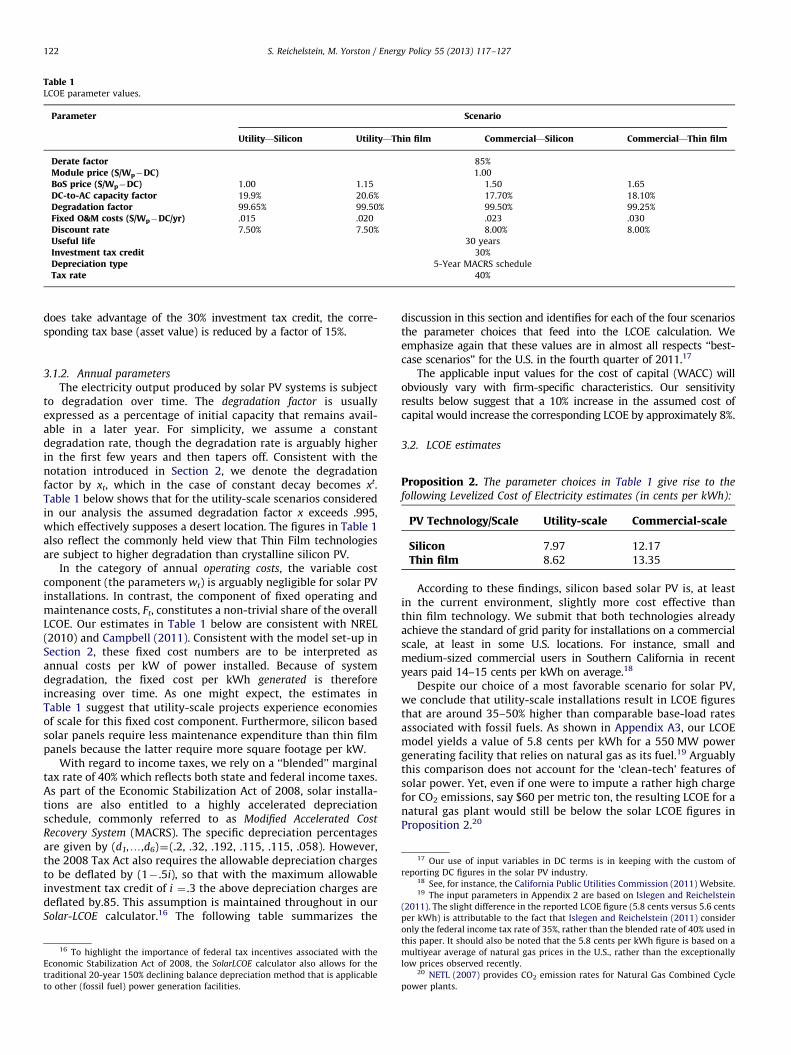
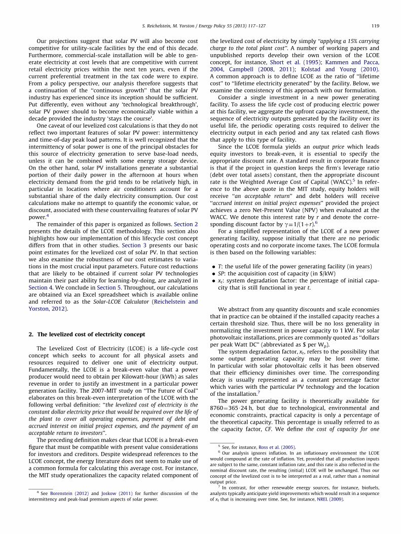
Table 1LCOE parameter values.

Parameter Scenario

Utility—Silicon Utility—Thin film Commercial—Silicon Commercial—Thin film

Derate factor 85%

Module price ($/Wp�DC) 1.00

BoS price ($/Wp�DC) 1.00 1.15 1.50 1.65

DC-to-AC capacity factor 19.9% 20.6% 17.70% 18.10%

Degradation factor 99.65% 99.50% 99.50% 99.25%

Fixed O&M costs ($/Wp�DC/yr) .015 .020 .023 .030

Discount rate 7.50% 7.50% 8.00% 8.00%

Useful life 30 years

Investment tax credit 30%

Depreciation type 5-Year MACRS schedule

Tax rate 40%

S. Reichelstein, M. Yorston / Energy Policy 55 (2013) 117–127122

does take advantage of the 30% investment tax credit, the corre-sponding tax base (asset value) is reduced by a factor of 15%.

17 Our use of input variables in DC terms is in keeping with the custom of

reporting DC figures in the solar PV industry.18 See, for instance, the California Public Utilities Commission (2011) Website.19 The input parameters in Appendix 2 are based on Islegen and Reichelstein

(2011). The slight difference in the reported LCOE figure (5.8 cents versus 5.6 cents

per kWh) is attributable to the fact that Islegen and Reichelstein (2011) consider

3.1.2. Annual parameters

The electricity output produced by solar PV systems is subjectto degradation over time. The degradation factor is usuallyexpressed as a percentage of initial capacity that remains avail-able in a later year. For simplicity, we assume a constantdegradation rate, though the degradation rate is arguably higherin the first few years and then tapers off. Consistent with thenotation introduced in Section 2, we denote the degradationfactor by xt, which in the case of constant decay becomes xt.Table 1 below shows that for the utility-scale scenarios consideredin our analysis the assumed degradation factor x exceeds .995,which effectively supposes a desert location. The figures in Table 1also reflect the commonly held view that Thin Film technologiesare subject to higher degradation than crystalline silicon PV.

In the category of annual operating costs, the variable costcomponent (the parameters wt) is arguably negligible for solar PVinstallations. In contrast, the component of fixed operating andmaintenance costs, Ft, constitutes a non-trivial share of the overallLCOE. Our estimates in Table 1 below are consistent with NREL(2010) and Campbell (2011). Consistent with the model set-up inSection 2, these fixed cost numbers are to be interpreted asannual costs per kW of power installed. Because of systemdegradation, the fixed cost per kWh generated is thereforeincreasing over time. As one might expect, the estimates inTable 1 suggest that utility-scale projects experience economiesof scale for this fixed cost component. Furthermore, silicon basedsolar panels require less maintenance expenditure than thin filmpanels because the latter require more square footage per kW.

With regard to income taxes, we rely on a ‘‘blended’’ marginaltax rate of 40% which reflects both state and federal income taxes.As part of the Economic Stabilization Act of 2008, solar installa-tions are also entitled to a highly accelerated depreciationschedule, commonly referred to as Modified Accelerated Cost

Recovery System (MACRS). The specific depreciation percentagesare given by (d1,y,d6)¼(.2, .32, .192, .115, .115, .058). However,the 2008 Tax Act also requires the allowable depreciation chargesto be deflated by (1� .5i), so that with the maximum allowableinvestment tax credit of i ¼ .3 the above depreciation charges aredeflated by.85. This assumption is maintained throughout in ourSolar-LCOE calculator.16 The following table summarizes the

16 To highlight the importance of federal tax incentives associated with the

Economic Stabilization Act of 2008, the SolarLCOE calculator also allows for the

traditional 20-year 150% declining balance depreciation method that is applicable

to other (fossil fuel) power generation facilities.

discussion in this section and identifies for each of the four scenariosthe parameter choices that feed into the LCOE calculation. Weemphasize again that these values are in almost all respects ‘‘best-case scenarios’’ for the U.S. in the fourth quarter of 2011.17

The applicable input values for the cost of capital (WACC) willobviously vary with firm-specific characteristics. Our sensitivityresults below suggest that a 10% increase in the assumed cost ofcapital would increase the corresponding LCOE by approximately 8%.

3.2. LCOE estimates

Proposition 2. The parameter choices in Table 1 give rise to the

following Levelized Cost of Electricity estimates (in cents per kWh):

only the federal income tax rate of

this paper. It should also be noted

multiyear average of natural gas p

low prices observed recently.20 NETL (2007) provides CO2 e

power plants.

35%, rather than the b

that the 5.8 cents per

rices in the U.S., rath

mission rates for Na

PV Technology/Scale

Utility-scale Commercial-scale

Silicon

7.97 12.17 Thin film 8.62 13.35

According to these findings, silicon based solar PV is, at leastin the current environment, slightly more cost effective thanthin film technology. We submit that both technologies alreadyachieve the standard of grid parity for installations on a commercialscale, at least in some U.S. locations. For instance, small andmedium-sized commercial users in Southern California in recentyears paid 14–15 cents per kWh on average.18

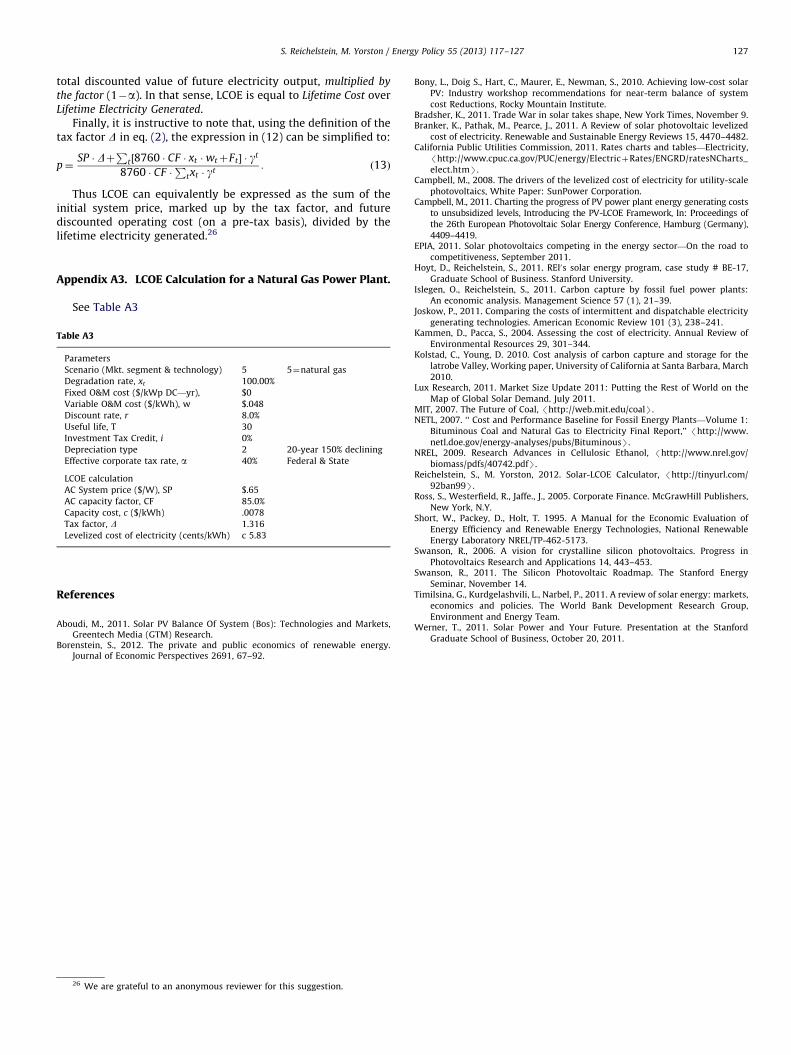
Despite our choice of a most favorable scenario for solar PV,we conclude that utility-scale installations result in LCOE figuresthat are around 35–50% higher than comparable base-load ratesassociated with fossil fuels. As shown in Appendix A3, our LCOEmodel yields a value of 5.8 cents per kWh for a 550 MW powergenerating facility that relies on natural gas as its fuel.19 Arguablythis comparison does not account for the ‘clean-tech’ features ofsolar power. Yet, even if one were to impute a rather high chargefor CO2 emissions, say $60 per metric ton, the resulting LCOE for anatural gas plant would still be below the solar LCOE figures inProposition 2.20

lended rate of 40% used in

kWh figure is based on a

er than the exceptionally

tural Gas Combined Cycle

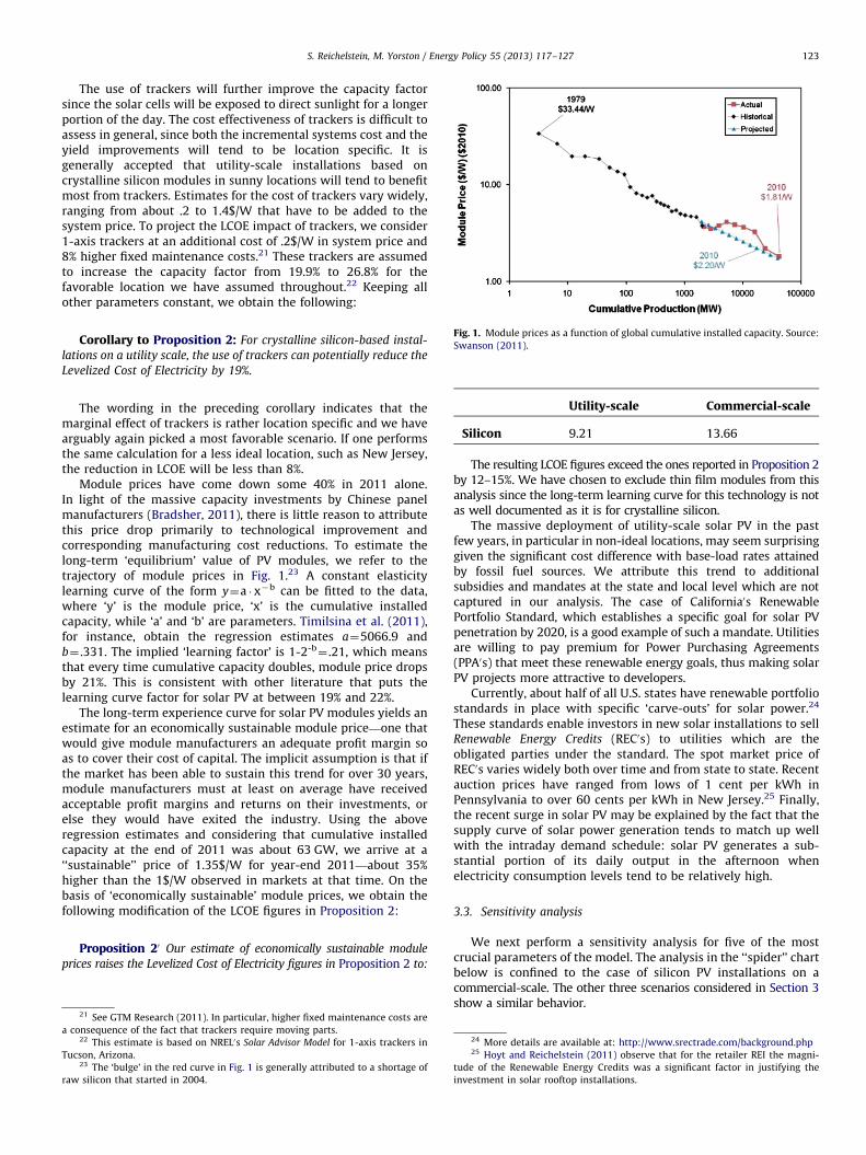
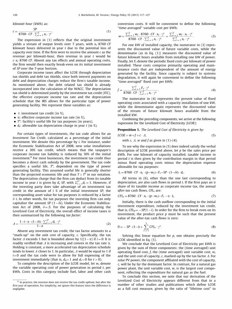
Fig. 1. Module prices as a function of global cumulative installed capacity. Source:

Swanson (2011).

S. Reichelstein, M. Yorston / Energy Policy 55 (2013) 117–127 123

The use of trackers will further improve the capacity factorsince the solar cells will be exposed to direct sunlight for a longerportion of the day. The cost effectiveness of trackers is difficult toassess in general, since both the incremental systems cost and theyield improvements will tend to be location specific. It isgenerally accepted that utility-scale installations based oncrystalline silicon modules in sunny locations will tend to benefitmost from trackers. Estimates for the cost of trackers vary widely,ranging from about .2 to 1.4$/W that have to be added to thesystem price. To project the LCOE impact of trackers, we consider1-axis trackers at an additional cost of .2$/W in system price and8% higher fixed maintenance costs.21 These trackers are assumedto increase the capacity factor from 19.9% to 26.8% for thefavorable location we have assumed throughout.22 Keeping allother parameters constant, we obtain the following:

Corollary to Proposition 2: For crystalline silicon-based instal-

lations on a utility scale, the use of trackers can potentially reduce the

Levelized Cost of Electricity by 19%.

The wording in the preceding corollary indicates that themarginal effect of trackers is rather location specific and we havearguably again picked a most favorable scenario. If one performsthe same calculation for a less ideal location, such as New Jersey,the reduction in LCOE will be less than 8%.

Module prices have come down some 40% in 2011 alone.In light of the massive capacity investments by Chinese panelmanufacturers (Bradsher, 2011), there is little reason to attributethis price drop primarily to technological improvement andcorresponding manufacturing cost reductions. To estimate thelong-term ‘equilibrium’ value of PV modules, we refer to thetrajectory of module prices in Fig. 1.23 A constant elasticitylearning curve of the form y¼a � x�b can be fitted to the data,where ‘y’ is the module price, ‘x’ is the cumulative installedcapacity, while ‘a’ and ‘b’ are parameters. Timilsina et al. (2011),for instance, obtain the regression estimates a¼5066.9 andb¼ .331. The implied ‘learning factor’ is 1-2-b

¼ .21, which meansthat every time cumulative capacity doubles, module price dropsby 21%. This is consistent with other literature that puts thelearning curve factor for solar PV at between 19% and 22%.

The long-term experience curve for solar PV modules yields anestimate for an economically sustainable module price—one thatwould give module manufacturers an adequate profit margin soas to cover their cost of capital. The implicit assumption is that ifthe market has been able to sustain this trend for over 30 years,module manufacturers must at least on average have receivedacceptable profit margins and returns on their investments, orelse they would have exited the industry. Using the aboveregression estimates and considering that cumulative installedcapacity at the end of 2011 was about 63 GW, we arrive at a‘‘sustainable’’ price of 1.35$/W for year-end 2011—about 35%higher than the 1$/W observed in markets at that time. On thebasis of ‘economically sustainable’ module prices, we obtain thefollowing modification of the LCOE figures in Proposition 2:

Proposition 20 Our estimate of economically sustainable module

prices raises the Levelized Cost of Electricity figures in Proposition 2 to:

21 See GTM Research (2011). In particular, higher fixed maintenance costs are

a consequence of the fact that trackers require moving parts.22 This estimate is based on NREL0s Solar Advisor Model for 1-axis trackers in

Tucson, Arizona.23 The ‘bulge’ in the red curve in Fig. 1 is generally attributed to a shortage of

raw silicon that started in 2004.

24 More details are a25 Hoyt and Reichels

tude of the Renewable E

investment in solar rooft

vailable at: http://www.srectra

tein (2011) observe that for th

nergy Credits was a significan

op installations.

Utility-scale

Commercial-scale

Silicon

9.21 13.66

The resulting LCOE figures exceed the ones reported in Proposition 2by 12–15%. We have chosen to exclude thin film modules from thisanalysis since the long-term learning curve for this technology is notas well documented as it is for crystalline silicon.

The massive deployment of utility-scale solar PV in the pastfew years, in particular in non-ideal locations, may seem surprisinggiven the significant cost difference with base-load rates attainedby fossil fuel sources. We attribute this trend to additionalsubsidies and mandates at the state and local level which are notcaptured in our analysis. The case of California0s RenewablePortfolio Standard, which establishes a specific goal for solar PVpenetration by 2020, is a good example of such a mandate. Utilitiesare willing to pay premium for Power Purchasing Agreements(PPA0s) that meet these renewable energy goals, thus making solarPV projects more attractive to developers.

Currently, about half of all U.S. states have renewable portfoliostandards in place with specific ‘carve-outs’ for solar power.24

These standards enable investors in new solar installations to sellRenewable Energy Credits (REC0s) to utilities which are theobligated parties under the standard. The spot market price ofREC0s varies widely both over time and from state to state. Recentauction prices have ranged from lows of 1 cent per kWh inPennsylvania to over 60 cents per kWh in New Jersey.25 Finally,the recent surge in solar PV may be explained by the fact that thesupply curve of solar power generation tends to match up wellwith the intraday demand schedule: solar PV generates a sub-stantial portion of its daily output in the afternoon whenelectricity consumption levels tend to be relatively high.

3.3. Sensitivity analysis

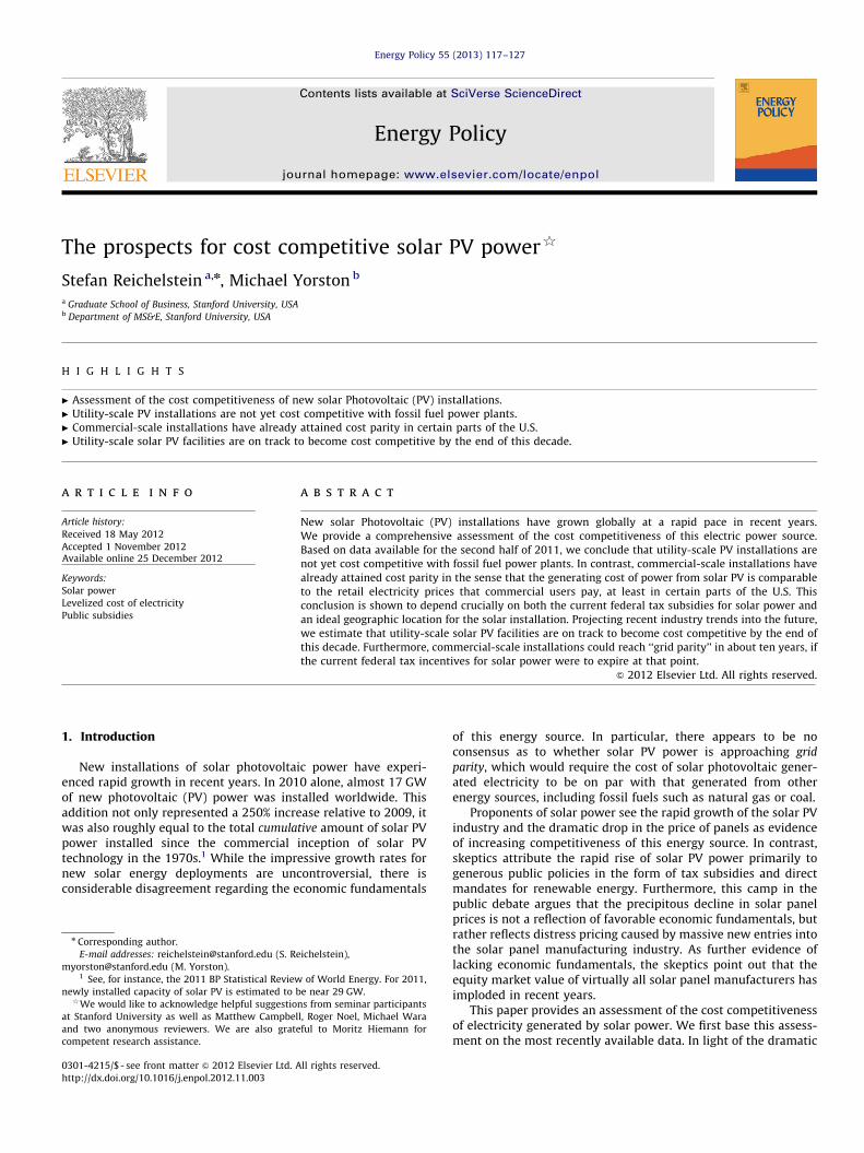
We next perform a sensitivity analysis for five of the mostcrucial parameters of the model. The analysis in the ‘‘spider’’ chartbelow is confined to the case of silicon PV installations on acommercial-scale. The other three scenarios considered in Section 3show a similar behavior.

de.com/background.php

e retailer REI the magni-

t factor in justifying the

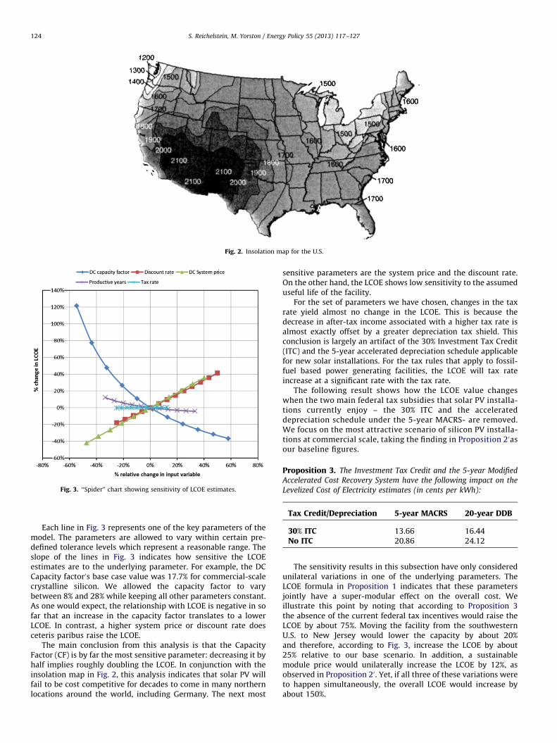
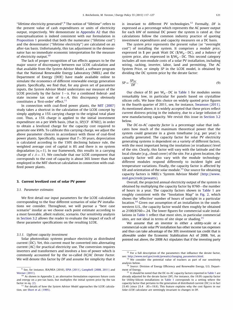
Fig. 3. ‘‘Spider’’ chart showing sensitivity of LCOE estimates.

Fig. 2. Insolation map for the U.S.

S. Reichelstein, M. Yorston / Energy Policy 55 (2013) 117–127124

Each line in Fig. 3 represents one of the key parameters of themodel. The parameters are allowed to vary within certain pre-defined tolerance levels which represent a reasonable range. Theslope of the lines in Fig. 3 indicates how sensitive the LCOEestimates are to the underlying parameter. For example, the DCCapacity factor0s base case value was 17.7% for commercial-scalecrystalline silicon. We allowed the capacity factor to varybetween 8% and 28% while keeping all other parameters constant.As one would expect, the relationship with LCOE is negative in sofar that an increase in the capacity factor translates to a lowerLCOE. In contrast, a higher system price or discount rate doesceteris paribus raise the LCOE.

The main conclusion from this analysis is that the CapacityFactor (CF) is by far the most sensitive parameter: decreasing it byhalf implies roughly doubling the LCOE. In conjunction with theinsolation map in Fig. 2, this analysis indicates that solar PV willfail to be cost competitive for decades to come in many northernlocations around the world, including Germany. The next most

sensitive parameters are the system price and the discount rate.On the other hand, the LCOE shows low sensitivity to the assumeduseful life of the facility.

For the set of parameters we have chosen, changes in the taxrate yield almost no change in the LCOE. This is because thedecrease in after-tax income associated with a higher tax rate isalmost exactly offset by a greater depreciation tax shield. Thisconclusion is largely an artifact of the 30% Investment Tax Credit(ITC) and the 5-year accelerated depreciation schedule applicablefor new solar installations. For the tax rules that apply to fossil-fuel based power generating facilities, the LCOE will tax rateincrease at a significant rate with the tax rate.

The following result shows how the LCOE value changeswhen the two main federal tax subsidies that solar PV installa-tions currently enjoy – the 30% ITC and the accelerateddepreciation schedule under the 5-year MACRS- are removed.We focus on the most attractive scenario of silicon PV installa-tions at commercial scale, taking the finding in Proposition 20asour baseline figures.

Proposition 3. The Investment Tax Credit and the 5-year Modified

Accelerated Cost Recovery System have the following impact on the

Levelized Cost of Electricity estimates (in cents per kWh):

Tax Credit/Depreciation

5-year MACRS 20-year DDB

30% ITC

13.66 16.44 No ITC 20.86 24.12

The sensitivity results in this subsection have only considered

unilateral variations in one of the underlying parameters. TheLCOE formula in Proposition 1 indicates that these parametersjointly have a super-modular effect on the overall cost. Weillustrate this point by noting that according to Proposition 3the absence of the current federal tax incentives would raise theLCOE by about 75%. Moving the facility from the southwesternU.S. to New Jersey would lower the capacity by about 20%and therefore, according to Fig. 3, increase the LCOE by about25% relative to our base scenario. In addition, a sustainablemodule price would unilaterally increase the LCOE by 12%, asobserved in Proposition 20. Yet, if all three of these variations wereto happen simultaneously, the overall LCOE would increase byabout 150%.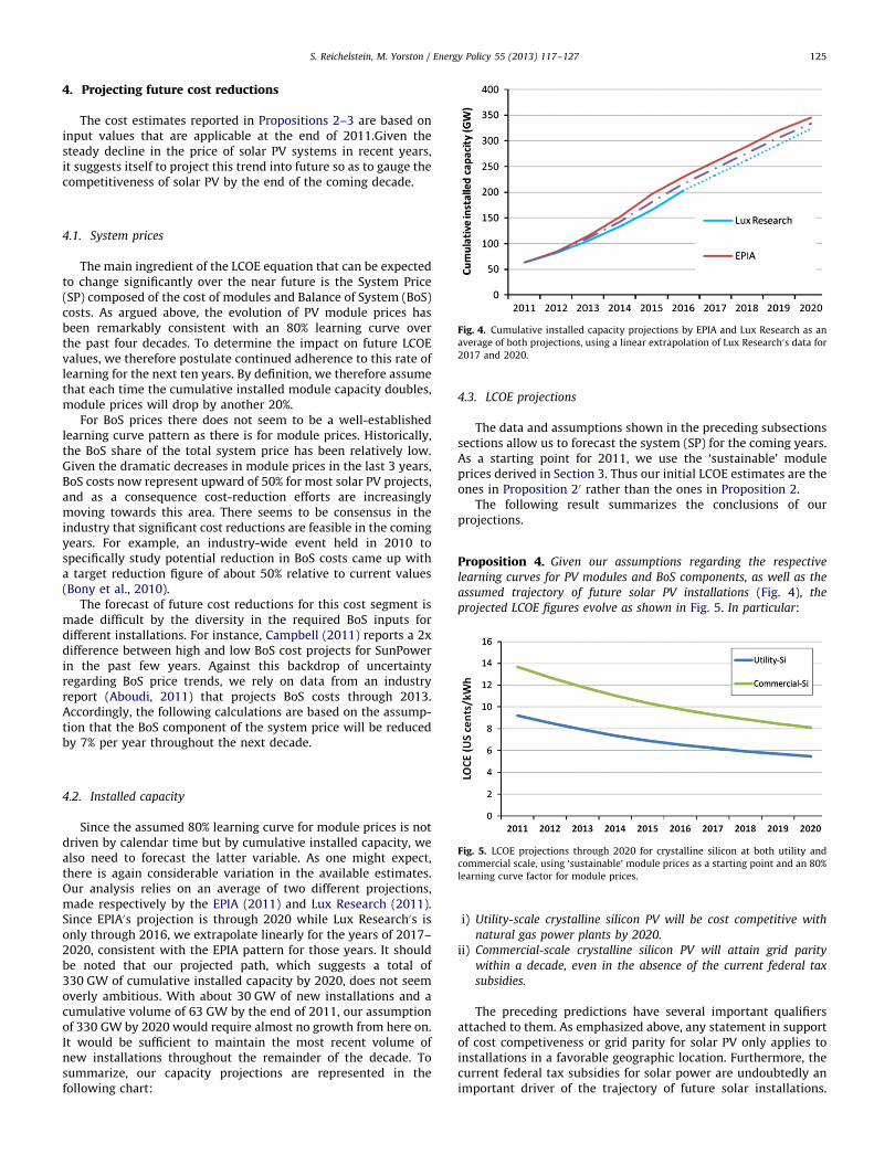

S. Reichelstein, M. Yorston / Energy Policy 55 (2013) 117–127 125

4. Projecting future cost reductions

The cost estimates reported in Propositions 2–3 are based oninput values that are applicable at the end of 2011.Given thesteady decline in the price of solar PV systems in recent years,it suggests itself to project this trend into future so as to gauge thecompetitiveness of solar PV by the end of the coming decade.

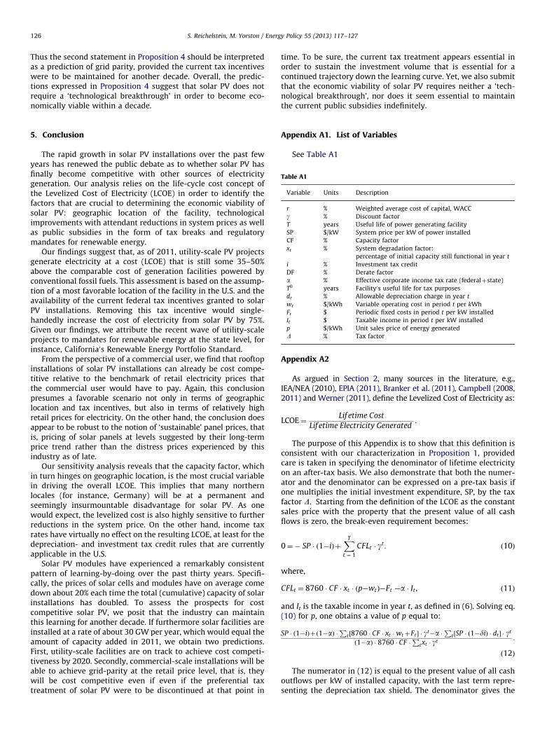
Fig. 4. Cumulative installed capacity projections by EPIA and Lux Research as an

average of both projections, using a linear extrapolation of Lux Research0s data for

2017 and 2020.

4.1. System prices

The main ingredient of the LCOE equation that can be expectedto change significantly over the near future is the System Price(SP) composed of the cost of modules and Balance of System (BoS)costs. As argued above, the evolution of PV module prices hasbeen remarkably consistent with an 80% learning curve overthe past four decades. To determine the impact on future LCOEvalues, we therefore postulate continued adherence to this rate oflearning for the next ten years. By definition, we therefore assumethat each time the cumulative installed module capacity doubles,module prices will drop by another 20%.

For BoS prices there does not seem to be a well-establishedlearning curve pattern as there is for module prices. Historically,the BoS share of the total system price has been relatively low.Given the dramatic decreases in module prices in the last 3 years,BoS costs now represent upward of 50% for most solar PV projects,and as a consequence cost-reduction efforts are increasinglymoving towards this area. There seems to be consensus in theindustry that significant cost reductions are feasible in the comingyears. For example, an industry-wide event held in 2010 tospecifically study potential reduction in BoS costs came up witha target reduction figure of about 50% relative to current values(Bony et al., 2010).

The forecast of future cost reductions for this cost segment ismade difficult by the diversity in the required BoS inputs fordifferent installations. For instance, Campbell (2011) reports a 2xdifference between high and low BoS cost projects for SunPowerin the past few years. Against this backdrop of uncertaintyregarding BoS price trends, we rely on data from an industryreport (Aboudi, 2011) that projects BoS costs through 2013.Accordingly, the following calculations are based on the assump-tion that the BoS component of the system price will be reducedby 7% per year throughout the next decade.

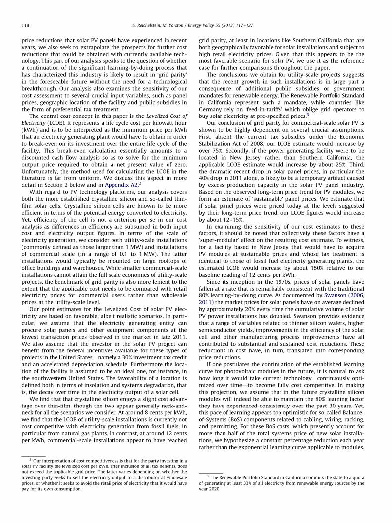
Fig. 5. LCOE projections through 2020 for crystalline silicon at both utility and

commercial scale, using ‘sustainable’ module prices as a starting point and an 80%

learning curve factor for module prices.

4.2. Installed capacity

Since the assumed 80% learning curve for module prices is notdriven by calendar time but by cumulative installed capacity, wealso need to forecast the latter variable. As one might expect,there is again considerable variation in the available estimates.Our analysis relies on an average of two different projections,made respectively by the EPIA (2011) and Lux Research (2011).Since EPIA0s projection is through 2020 while Lux Research0s isonly through 2016, we extrapolate linearly for the years of 2017–2020, consistent with the EPIA pattern for those years. It shouldbe noted that our projected path, which suggests a total of330 GW of cumulative installed capacity by 2020, does not seemoverly ambitious. With about 30 GW of new installations and acumulative volume of 63 GW by the end of 2011, our assumptionof 330 GW by 2020 would require almost no growth from here on.It would be sufficient to maintain the most recent volume ofnew installations throughout the remainder of the decade. Tosummarize, our capacity projections are represented in thefollowing chart:

4.3. LCOE projections

The data and assumptions shown in the preceding subsectionssections allow us to forecast the system (SP) for the coming years.As a starting point for 2011, we use the ‘sustainable’ moduleprices derived in Section 3. Thus our initial LCOE estimates are theones in Proposition 20 rather than the ones in Proposition 2.

The following result summarizes the conclusions of ourprojections.

Proposition 4. Given our assumptions regarding the respective

learning curves for PV modules and BoS components, as well as the

assumed trajectory of future solar PV installations (Fig. 4), the

projected LCOE figures evolve as shown in Fig. 5. In particular:

i)

Utility-scale crystalline silicon PV will be cost competitive with

natural gas power plants by 2020.

ii)

Commercial-scale crystalline silicon PV will attain grid parity

within a decade, even in the absence of the current federal tax

subsidies.

The preceding predictions have several important qualifiersattached to them. As emphasized above, any statement in supportof cost competiveness or grid parity for solar PV only applies toinstallations in a favorable geographic location. Furthermore, thecurrent federal tax subsidies for solar power are undoubtedly animportant driver of the trajectory of future solar installations.

S. Reichelstein, M. Yorston / Energy Policy 55 (2013) 117–127126

Thus the second statement in Proposition 4 should be interpretedas a prediction of grid parity, provided the current tax incentiveswere to be maintained for another decade. Overall, the predic-tions expressed in Proposition 4 suggest that solar PV does notrequire a ‘technological breakthrough’ in order to become eco-nomically viable within a decade.

Table A1

Variable Units Description

r % Weighted average cost of capital, WACC

g % Discount factor

T years Useful life of power generating facility

SP $/kW System price per kW of power installed

CF % Capacity factor

xt % System degradation factor:

percentage of initial capacity still functional in year t

i % Investment tax credit

DF % Derate factor

a % Effective corporate income tax rate (federalþstate)

T0 years Facility0s useful life for tax purposes

dt % Allowable depreciation charge in year t

wt $/kWh Variable operating cost in period t per kWh

Ft $ Periodic fixed costs in period t per kW installed

It $ Taxable income in period t per kW installed

p $/kWh Unit sales price of energy generated

D % Tax factor

5. Conclusion

The rapid growth in solar PV installations over the past fewyears has renewed the public debate as to whether solar PV hasfinally become competitive with other sources of electricitygeneration. Our analysis relies on the life-cycle cost concept ofthe Levelized Cost of Electricity (LCOE) in order to identify thefactors that are crucial to determining the economic viability ofsolar PV: geographic location of the facility, technologicalimprovements with attendant reductions in system prices as wellas public subsidies in the form of tax breaks and regulatorymandates for renewable energy.

Our findings suggest that, as of 2011, utility-scale PV projectsgenerate electricity at a cost (LCOE) that is still some 35–50%above the comparable cost of generation facilities powered byconventional fossil fuels. This assessment is based on the assump-tion of a most favorable location of the facility in the U.S. and theavailability of the current federal tax incentives granted to solarPV installations. Removing this tax incentive would single-handedly increase the cost of electricity from solar PV by 75%.Given our findings, we attribute the recent wave of utility-scaleprojects to mandates for renewable energy at the state level, forinstance, California0s Renewable Energy Portfolio Standard.

From the perspective of a commercial user, we find that rooftopinstallations of solar PV installations can already be cost compe-titive relative to the benchmark of retail electricity prices thatthe commercial user would have to pay. Again, this conclusionpresumes a favorable scenario not only in terms of geographiclocation and tax incentives, but also in terms of relatively highretail prices for electricity. On the other hand, the conclusion doesappear to be robust to the notion of ‘sustainable’ panel prices, thatis, pricing of solar panels at levels suggested by their long-termprice trend rather than the distress prices experienced by thisindustry as of late.

Our sensitivity analysis reveals that the capacity factor, whichin turn hinges on geographic location, is the most crucial variablein driving the overall LCOE. This implies that many northernlocales (for instance, Germany) will be at a permanent andseemingly insurmountable disadvantage for solar PV. As onewould expect, the levelized cost is also highly sensitive to furtherreductions in the system price. On the other hand, income taxrates have virtually no effect on the resulting LCOE, at least for thedepreciation- and investment tax credit rules that are currentlyapplicable in the U.S.

Solar PV modules have experienced a remarkably consistentpattern of learning-by-doing over the past thirty years. Specifi-cally, the prices of solar cells and modules have on average comedown about 20% each time the total (cumulative) capacity of solarinstallations has doubled. To assess the prospects for costcompetitive solar PV, we posit that the industry can maintainthis learning for another decade. If furthermore solar facilities areinstalled at a rate of about 30 GW per year, which would equal theamount of capacity added in 2011, we obtain two predictions.First, utility-scale facilities are on track to achieve cost competi-tiveness by 2020. Secondly, commercial-scale installations will beable to achieve grid-parity at the retail price level, that is, theywill be cost competitive even if even if the preferential taxtreatment of solar PV were to be discontinued at that point in

time. To be sure, the current tax treatment appears essential inorder to sustain the investment volume that is essential for acontinued trajectory down the learning curve. Yet, we also submitthat the economic viability of solar PV requires neither a ‘tech-nological breakthrough’, nor does it seem essential to maintainthe current public subsidies indefinitely.

Appendix A1. List of Variables

See Table A1

Appendix A2

As argued in Section 2, many sources in the literature, e.g.,IEA/NEA (2010), EPIA (2011), Branker et al. (2011), Campbell (2008,2011) and Werner (2011), define the Levelized Cost of Electricity as:

LCOE¼Lif etime Cost

Lif etime Electricity Generated:

The purpose of this Appendix is to show that this definition isconsistent with our characterization in Proposition 1, providedcare is taken in specifying the denominator of lifetime electricityon an after-tax basis. We also demonstrate that both the numer-ator and the denominator can be expressed on a pre-tax basis ifone multiplies the initial investment expenditure, SP, by the taxfactor D. Starting from the definition of the LCOE as the constantsales price with the property that the present value of all cashflows is zero, the break-even requirement becomes:

0¼� SP � 1�ið ÞþXT

t ¼ 1

CFLt � gt : ð10Þ

where,

CFLt ¼ 8760 � CF � xt � p�wtð Þ�Ft �a � It , ð11Þ

and It is the taxable income in year t, as defined in (6). Solving eq.(10) for p, one obtains a value of p equal to:

SP � 1�ið Þþ 1�að Þ �P

t ½8760 � CF � xt �wtþFt � � gt�a �P

t½SP � 1�dið Þ � dt� � gt

1�að Þ � 8760 � CF �P

txt � gt:

ð12Þ

The numerator in (12) is equal to the present value of all cashoutflows per kW of installed capacity, with the last term repre-senting the depreciation tax shield. The denominator gives the

S. Reichelstein, M. Yorston / Energy Policy 55 (2013) 117–127 127

total discounted value of future electricity output, multiplied by

the factor (1�a). In that sense, LCOE is equal to Lifetime Cost overLifetime Electricity Generated.

Finally, it is instructive to note that, using the definition of thetax factor D in eq. (2), the expression in (12) can be simplified to:

p¼SP � Dþ

Pt½8760 � CF � xt �wtþFt� � gt

8760 � CF �P

txt � gt: ð13Þ

Thus LCOE can equivalently be expressed as the sum of theinitial system price, marked up by the tax factor, and futurediscounted operating cost (on a pre-tax basis), divided by thelifetime electricity generated.26

Appendix A3. LCOE Calculation for a Natural Gas Power Plant.

See Table A3

Table A3

Parameters

Scenario (Mkt. segment & technology) 5 5¼natural gas

Degradation rate, xt 100.00%

Fixed O&M cost ($/kWp DC—yr), $0

Variable O&M cost ($/kWh), w $.048

Discount rate, r 8.0%

Useful life, T 30

Investment Tax Credit, i 0%

Depreciation type 2 20-year 150% declining

Effective corporate tax rate, a 40% Federal & State

LCOE calculation

AC System price ($/W), SP $.65

AC capacity factor, CF 85.0%

Capacity cost, c ($/kWh) .0078

Tax factor, D 1.316

Levelized cost of electricity (cents/kWh) c 5.83

References

Aboudi, M., 2011. Solar PV Balance Of System (Bos): Technologies and Markets,Greentech Media (GTM) Research.

Borenstein, S., 2012. The private and public economics of renewable energy.Journal of Economic Perspectives 2691, 67–92.

26 We are grateful to an anonymous reviewer for this suggestion.

Bony, L., Doig S., Hart, C., Maurer, E., Newman, S., 2010. Achieving low-cost solarPV: Industry workshop recommendations for near-term balance of systemcost Reductions, Rocky Mountain Institute.

Bradsher, K., 2011. Trade War in solar takes shape, New York Times, November 9.Branker, K., Pathak, M., Pearce, J., 2011. A Review of solar photovoltaic levelized

cost of electricity. Renewable and Sustainable Energy Reviews 15, 4470–4482.California Public Utilities Commission, 2011. Rates charts and tables—Electricity,

/http://www.cpuc.ca.gov/PUC/energy/ElectricþRates/ENGRD/ratesNCharts_elect.htmS.

Campbell, M., 2008. The drivers of the levelized cost of electricity for utility-scalephotovoltaics, White Paper: SunPower Corporation.

Campbell, M., 2011. Charting the progress of PV power plant energy generating coststo unsubsidized levels, Introducing the PV-LCOE Framework, In: Proceedings ofthe 26th European Photovoltaic Solar Energy Conference, Hamburg (Germany),4409–4419.

EPIA, 2011. Solar photovoltaics competing in the energy sector—On the road tocompetitiveness, September 2011.

Hoyt, D., Reichelstein, S., 2011. REI0s solar energy program, case study # BE-17,Graduate School of Business. Stanford University.

Islegen, O., Reichelstein, S., 2011. Carbon capture by fossil fuel power plants:An economic analysis. Management Science 57 (1), 21–39.

Joskow, P., 2011. Comparing the costs of intermittent and dispatchable electricitygenerating technologies. American Economic Review 101 (3), 238–241.

Kammen, D., Pacca, S., 2004. Assessing the cost of electricity. Annual Review ofEnvironmental Resources 29, 301–344.

Kolstad, C., Young, D. 2010. Cost analysis of carbon capture and storage for thelatrobe Valley, Working paper, University of California at Santa Barbara, March2010.

Lux Research, 2011. Market Size Update 2011: Putting the Rest of World on theMap of Global Solar Demand. July 2011.

MIT, 2007. The Future of Coal, /http://web.mit.edu/coalS.NETL, 2007. ‘‘ Cost and Performance Baseline for Fossil Energy Plants—Volume 1:

Bituminous Coal and Natural Gas to Electricity Final Report,’’ /http://www.netl.doe.gov/energy-analyses/pubs/BituminousS.

NREL, 2009. Research Advances in Cellulosic Ethanol, /http://www.nrel.gov/biomass/pdfs/40742.pdfS.

Reichelstein, S., M. Yorston, 2012. Solar-LCOE Calculator, /http://tinyurl.com/92ban99S.

Ross, S., Westerfield, R., Jaffe., J., 2005. Corporate Finance. McGrawHill Publishers,New York, N.Y.

Short, W., Packey, D., Holt, T. 1995. A Manual for the Economic Evaluation ofEnergy Efficiency and Renewable Energy Technologies, National RenewableEnergy Laboratory NREL/TP-462-5173.

Swanson, R., 2006. A vision for crystalline silicon photovoltaics. Progress inPhotovoltaics Research and Applications 14, 443–453.

Swanson, R., 2011. The Silicon Photovoltaic Roadmap. The Stanford EnergySeminar, November 14.

Timilsina, G., Kurdgelashvili, L., Narbel, P., 2011. A review of solar energy: markets,economics and policies. The World Bank Development Research Group,Environment and Energy Team.

Werner, T., 2011. Solar Power and Your Future. Presentation at the StanfordGraduate School of Business, October 20, 2011.