The Prothero and Robinson example: Convergence studies for

Joachim Rang

The Prothero andRobinson example:

Convergence studies forRunge–Kutta and

Rosenbrock–Wannermethods

Informatikbericht Nr. 2014-05

Institute of Scientific ComputingCarl-Friedrich-Gauß-FakultatTechnische Universitat Braunschweig

Braunschweig, Germany

http://www.digibib.tu-bs.de/?docid=00057194 13/08/2014

This document was created July 2014 using LATEX 2ε.

Institute of Scientific ComputingTechnische Universitat BraunschweigHans-Sommer-Straße 65D-38106 Braunschweig, Germany

url: www.wire.tu-bs.de

mail: [email protected]

e-print: http://www.digibib.tu-bs.de/?docid=00057194

Copyright c© by Joachim Rang

This work is subject to copyright. All rights are reserved, whether thewhole or part of the material is concerned, specifically the rights of transla-tion, reprinting, reuse of illustrations, recitation, broadcasting, reproductionon microfilm or in any other way, and storage in data banks. Duplicationof this publication or parts thereof is permitted in connection with reviewsor scholarly analysis. Permission for use must always be obtained from thecopyright holder.

Alle Rechte vorbehalten, auch das des auszugsweisen Nachdrucks, derauszugsweisen oder vollstandigen Wiedergabe (Photographie, Mikroskopie),der Speicherung in Datenverarbeitungsanlagen und das der Ubersetzung.


www.wire.tu-bs.de

mailto:[email protected]?subject=The Prothero and Robinson example: Convergence studies for Runge--Kutta and Rosenbrock--Wanner methods

The Prothero and Robinson example:

Convergence studies for Runge–Kutta and

Rosenbrock–Wanner methods

Joachim Rang

Institute of Scientific Computing, TU [email protected]

Abstract

It is well-known that one-step methods have order reduction ifthey are applied on stiff ODEs such as the example of Prothero–Robinson. In this paper we analyse the local error of Runge–Kuttaand Rosenbrock–Wanner methods. We derive new order conditions anddefine BPR-consistency. We show that for strongly A-stable methodsBPR-consistency implies BPR-convergence. Finally we analyse meth-ods from literature, derive new BPR-consistent methods and presentnumerical examples. This analysis shows that Runge–Kutta methodsand Rosenbrock–Wanner methods which are not stiffly accurate andare only consistent converge with order 2 in the stiff case, but the errorconstant may be large. As an improvement stiffly accurate methodscan be considered, since the numerical error is now smaller, but themethod converges only with order 1. The numerical results and theorder of convergence can be improved if the derived order conditionsare satisfied.

Keywords: example of Prothero–Robinson, order reduction, B-convergence, Runge–Kutta methods, Rosenbrock–Wanner methods,ODEs

i


mailto:[email protected]?subject=The Prothero and Robinson example: Convergence studies for Runge--Kutta and Rosenbrock--Wanner methods

ii


1 Introduction

In the simulation of stiff ODEs and differential algebraic equations (DAEs),Runge–Kutta (RK) and Rosenbrock–Wanner (ROW) methods seem to bea good choice since these classes of methods include A-stable schemes. A-stability guarantees in general a stable numerical solution. One disadvan-tage of one-step methods is the order reduction phenomenon for stiff prob-lems such as the example of Prothero and Robinson [17]. For fully implicitRunge–Kutta methods like Gauß–Legendre methods the numerical order ofconvergence decreases from 2s to s, where s is the number of internal stages.

Order reduction can be observed for other stiff ODEs, too, such as semi-discretised parabolic PDEs, often called MOL-ODEs. Analytical results areproven by Ostermann and Roche [15]. They show that implicit Runge–Kuttamethods may have a fractional order of convergence. Similar results arepresented for Rosenbrock–Wanner methods in [16].

For Runge–Kutta methods Frank, Schneid and Ueberhuber in [6] intro-duced the concept of B-consistency and B-convergence. They show thatB-consistency and B-stability imply B-convergence [7]. In contrast to the es-timates for non-stiff problems the local and the global error in the case of stiffproblems depend on a one-sided Lipschitz constant, and not on the classicalLipschitz constant. In several papers B-convergence of implicit Runge–Kuttamethods is studied. For an overview we refer to [8] and [9].

In contrast to implicit Runge–Kutta methods Rosenbrock–Wanner meth-ods can not be B-stable (see [9, 18] and the references cited in there). Scholzintroduces B-consistency for Rosenbrock–Wanner methods [24] and provesthat strongly A-stable Rosenbrock–Wanner methods are B-convergent if theyare B-consistent. Moreover, order conditions are presented such that B-consistent Rosenbrock–Wanner methods can be developed. A Rosenbrock–Wanner method satisfying these order conditions from Scholz is the RODASPmethod from Steinebach [26].

More or less all error bounds which can be found in literature estimate thelocal or global error w.r.t. powers of the step-size. It is well-known that, forexample, stiffly accurate Runge–Kutta methods such as Radau-IIA methodsthe local and global error can be estimated with τ q/z in the case of thestiff Prothero–Robinson example. Here τ denotes the step-size and z := τλ,where λ is the given stiffness. The factor τ q/z implies a numerical order ofconvergence of order q− 1. Since z is very large for very stiff problems theseerror terms are often smaller than the error terms of order τ q.

In this paper we introduce the concept of BPR-consistency and BPR-convergence similar to the concept of B-consistency and B-convergencefrom [6]. The only difference to [6] is that we concentrate only on the ex-

1


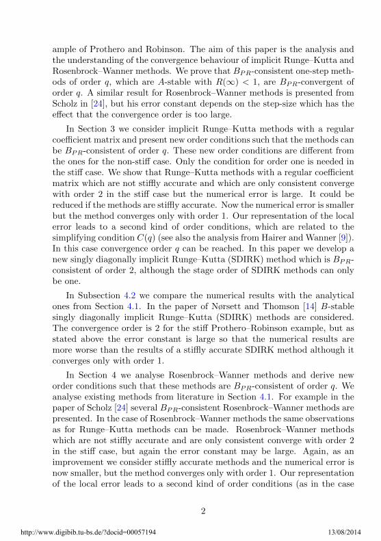
ample of Prothero and Robinson. The aim of this paper is the analysis andthe understanding of the convergence behaviour of implicit Runge–Kutta andRosenbrock–Wanner methods. We prove that BPR-consistent one-step meth-ods of order q, which are A-stable with R(∞) < 1, are BPR-convergent oforder q. A similar result for Rosenbrock–Wanner methods is presented fromScholz in [24], but his error constant depends on the step-size which has theeffect that the convergence order is too large.

In Section 3 we consider implicit Runge–Kutta methods with a regularcoefficient matrix and present new order conditions such that the methods canbe BPR-consistent of order q. These new order conditions are different fromthe ones for the non-stiff case. Only the condition for order one is needed inthe stiff case. We show that Runge–Kutta methods with a regular coefficientmatrix which are not stiffly accurate and which are only consistent convergewith order 2 in the stiff case but the numerical error is large. It could bereduced if the methods are stiffly accurate. Now the numerical error is smallerbut the method converges only with order 1. Our representation of the localerror leads to a second kind of order conditions, which are related to thesimplifying condition C(q) (see also the analysis from Hairer and Wanner [9]).In this case convergence order q can be reached. In this paper we develop anew singly diagonally implicit Runge–Kutta (SDIRK) method which is BPR-consistent of order 2, although the stage order of SDIRK methods can onlybe one.

In Subsection 4.2 we compare the numerical results with the analyticalones from Section 4.1. In the paper of Nørsett and Thomson [14] B-stablesingly diagonally implicit Runge–Kutta (SDIRK) methods are considered.The convergence order is 2 for the stiff Prothero–Robinson example, but asstated above the error constant is large so that the numerical results aremore worse than the results of a stiffly accurate SDIRK method although itconverges only with order 1.

In Section 4 we analyse Rosenbrock–Wanner methods and derive neworder conditions such that these methods are BPR-consistent of order q. Weanalyse existing methods from literature in Section 4.1. For example in thepaper of Scholz [24] several BPR-consistent Rosenbrock–Wanner methods arepresented. In the case of Rosenbrock–Wanner methods the same observationsas for Runge–Kutta methods can be made. Rosenbrock–Wanner methodswhich are not stiffly accurate and are only consistent converge with order 2in the stiff case, but again the error constant may be large. Again, as animprovement we consider stiffly accurate methods and the numerical error isnow smaller, but the method converges only with order 1. Our representationof the local error leads to a second kind of order conditions (as in the case

2


of Runge–Kutta methods) such that convergence order q can be reached. InSections 6.2 and 6.5 we compare the numerical results for 2nd and 3rd ordermethods with the analytical ones from Section 6.1 and 6.3.

Finally we summarise the results of the paper and give an outlook tofuture investigations.

2 BPR-consistency and BPR-convergence

2.1 The example of Prothero–Robinson

We start our considerations with the well-known example of Prothero andRobinson (see [17]), which is given by

u = λ(u− ϕ(t)) + ϕ(t), u(0) = ϕ(0), λ� 0, (1)

where u(t) = ϕ(t) is the exact solution of (1). One-step methods have usuallydifficulties to solve this problem because they often have order reduction if λis very small, i.e. the ODE is very stiff.

In the book of Hairer and Wanner [9] an analysis of the local error forRunge–Kutta methods applied on the ODE (1) can be found which showsthat the convergence order decreases from the convergence order p to thestage order q. Therefore, several papers deal with this phenomenon and tryto improve Runge–Kutta methods such that a better convergence order canbe obtained. For an overview we refer to the book of Hairer and Wanner [9]or to the book of Strehmel and Weiner [27].

In this paper we make a careful analysis of the local error so that we areable to understand the behaviour of different Runge–Kutta and Rosenbrock–Wanner methods. Moreover, we are interested in developing new order con-ditions which give us the possibility to increase the convergence order whenwe solve the stiff Prothero–Robinson example or other stiff ODEs and DAEs.Therefore, we want to adapt the idea of Frank, Schneid and Ueberhuberwho introduce the concept of B-consistency and B-convergence [6]. Since weare interested in a rigorous analysis of the Prothero–Robinson example werestrict ourselves to this problem.

2.2 BPR-consistency

Let us apply a one-step method on the example of Prothero and Robinsonand let z := τλ. For non-stiff problems we have τ → 0 and z → 0, and thelocal error can be computed in the usual way, where the Lipschitz conditionL of the rhs of the ODE is used. In the case of λ→ −∞ in equation (1) we

3


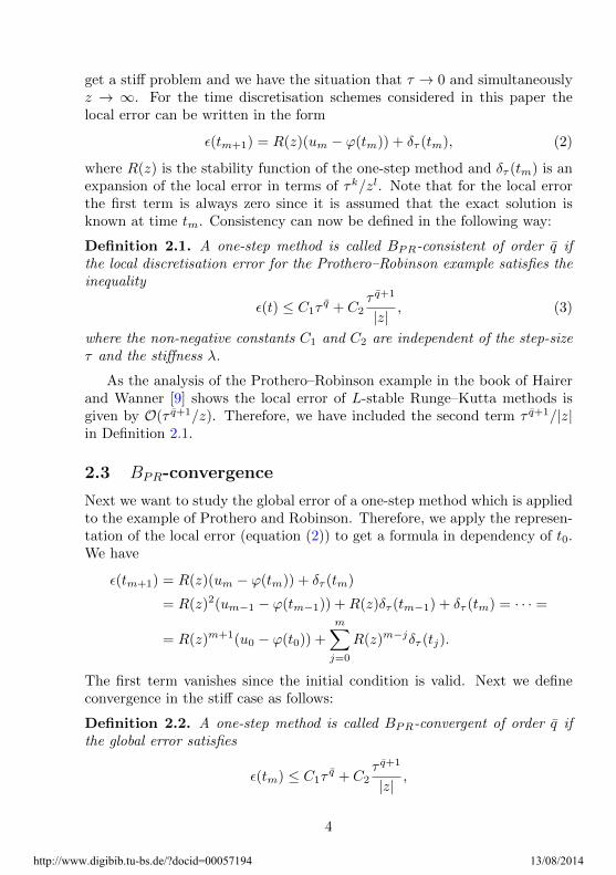
get a stiff problem and we have the situation that τ → 0 and simultaneouslyz → ∞. For the time discretisation schemes considered in this paper thelocal error can be written in the form

ε(tm+1) = R(z)(um − ϕ(tm)) + δτ (tm), (2)

where R(z) is the stability function of the one-step method and δτ (tm) is anexpansion of the local error in terms of τk/zl. Note that for the local errorthe first term is always zero since it is assumed that the exact solution isknown at time tm. Consistency can now be defined in the following way:

Definition 2.1. A one-step method is called BPR-consistent of order q ifthe local discretisation error for the Prothero–Robinson example satisfies theinequality

ε(t) ≤ C1τq + C2

τ q+1

|z|, (3)

where the non-negative constants C1 and C2 are independent of the step-sizeτ and the stiffness λ.

As the analysis of the Prothero–Robinson example in the book of Hairerand Wanner [9] shows the local error of L-stable Runge–Kutta methods isgiven by O(τ q+1/z). Therefore, we have included the second term τ q+1/|z|in Definition 2.1.

2.3 BPR-convergence

Next we want to study the global error of a one-step method which is appliedto the example of Prothero and Robinson. Therefore, we apply the represen-tation of the local error (equation (2)) to get a formula in dependency of t0.We have

ε(tm+1) = R(z)(um − ϕ(tm)) + δτ (tm)

= R(z)2(um−1 − ϕ(tm−1)) +R(z)δτ (tm−1) + δτ (tm) = · · · =

= R(z)m+1(u0 − ϕ(t0)) +m∑j=0

R(z)m−jδτ (tj).

The first term vanishes since the initial condition is valid. Next we defineconvergence in the stiff case as follows:

Definition 2.2. A one-step method is called BPR-convergent of order q ifthe global error satisfies

ε(tm) ≤ C1τq + C2

τ q+1

|z|,

4


where C1 and C2 are non-negative constants which are independent of thestep-size τ and the stiffness λ.

Next we show that BPR-consistency and A-stability imply BPR-convergence or, to be more precise, that BPR-consistency of order q andA-stability imply BPR-convergence of order q − 1. If the one-step methodis A-stable with R(∞) = 0 the converge order in the stiff case is q, too, ifequidistant time-steps are used.

Theorem 2.3. Consider an A-stable one-step method with R(∞) ≤ 1. As-sume that the local error can be written in the form (2) and that the one-stepmethod is BPR-consistent of order q + 1.

• Then the one-step method is BPR-convergent of order q.

• If R(∞) < 0 then for constant step-sizes τ the one-step method is BPR-convergent of order q + 1.

• If R(∞) = 0 the one-step method is BPR-convergent of order q + 1.

Proof. This theorem can be proven in an analogous way as in the case ofimplicit Runge–Kutta methods (see [9]). We start with an A-stable one-stepmethod and let ρ = R(∞). Then the global error reads as

ε(tm+1) =m∑j=0

ρm−jδτ (tj).

Since |ρ| ≤ 1 we have

|ε(tm+1)| ≤m∑j=0

|δτ (tj)| ≤ (m+ 1) maxj=0,...,m

|δτ (tj)|. (4)

Next the quantity δτ (tj) can be estimated with the help of inequality (3).Since m = (tm − t0)/τ we finally have

|ε(tm+1)| ≤ (tm − t0)

(C1τ

q + C2τ q+1

z

)and we have proven the first statement.

5


If ρ < 0 we can improve our last estimate if constant step-sizes τ are used.In this case we have

ε(tm+1) =

m∑j=0

[ρm−j ±

m−j−1∑k=0

ρk

]δτ (tj)

=m∑k=0

ρkδτ (t0) +m∑j=1

m−j∑k=0

ρk(δτ (tj)− δτ (tj−1)).

Withm∑k=0

ρk =1− ρm+1

1− ρ

it follows

ε(tm+1) =1− ρm+1

1− ρδτ (t0) +

m∑j=1

1− ρm−j+1

1− ρ(δτ (tj)− δτ (tj−1)).

Sinceδτ (tj)− δτ (tj−1) = τ δτ (tj−1) +O(τ2)

we finally get

δτ (tm+1) ≤ C1τq+1 + C2

τ q+2

z

and have proven the second statement. In the case of an L-stable methodthe global error reads as

ε(tm+1) = δτ (tm),

i.e. the global error is equal to the local one.

The estimate (4) is not sharp, but we are only interested in an estimatew.r.t. to potentials of τ . As in the paper of Scholz [24] the geometrical seriescan be applied, but that technique has the only effect that the error constantsare smaller.

3 Runge–Kutta methods

3.1 Application to ODEs

We start our considerations with an initial value problem of the form

u = F (t,u), u(0) = u0. (5)

6


A Runge–Kutta (RK) method with s internal stages [9, 27] is a one–step–method for solving (5) of the form

ki = F

tm + αiτm,um + τm

s∑j=1

aijkj

, i = 1, . . . , s, (6)

um+1 = um + τm

s∑i=1

biki. (7)

Coefficients of the Runge–Kutta method are aij , bi and ci and should bechosen in such a way that some order conditions are satisfied to obtain a suf-ficient high consistency order. In the following we assume that the coefficientmatrix A = (aij)

si,j=1 is regular. For example fully implicit Runge–Kutta

methods like Radau-IIA methods or diagonally implicit Runge–Kutta meth-ods without an explicit first stage are met this condition.

If we apply a Runge–Kutta method on the problem of Dahlquist [3], i.e.on u = λu with λ ∈ C and Re λ < 0, the stability function of the Runge–Kutta method R(z), z := λτ can be computed. The stability function isgiven by

R(z) = 1 + zb(I − zA)−1e,

where e := (1, . . . , 1)> ∈ Rs, b := (b1, . . . , bs)> and A := (aij)

si,j=1. The

Runge–Kutta method is called A-stable if |R(z)| ≤ 1 for all z ∈ C−. If,furthermore, R(∞) < 1 the Runge–Kutta method is called strongly A-stableand L-stable if R(∞) = 0 (see [4]).

The property A-stability implies that a Runge–Kutta method is dissipa-tive for Dahlquist’s problem. But what happens if non-linear problems aresolved? For this case B-stability may be important. Runge–Kutta methodsare B-stable if they are algebraically stable, i.e. if the matrices

B = diag(b1, . . . , bs) and M = BA + A>B− bb>

are positive semi-definite. For example the Gauß-Legendre, the Radau-IA,the Radau-IIA, and the Lobatto-IIIC methods are algebraically stable.

3.2 Local error

Next we apply the Runge–Kutta method (6)–(7) on the example of Protheroand Robinson, i.e. on equation (1). First we get

ki = λ

um + τs∑j=1

aijkj − ϕ(tm + ciτ)

+ ϕ(tm + ciτ).

7


In the following we use the abbreviations

ϕ(k)i := ϕ(k)(tm + αiτ), i = 1, . . . , s, ϕ(k)

m := ϕ(k)(tm), k ≥ 0,

Φ(k) := (ϕ(k)1 , . . . , ϕ(k)

s )>, k := (k1, . . . , ks)>, c := (c1, . . . , cs)

>.

It follows

ki = λ

um + τs∑j=1

aijkj − ϕi

+ ϕi.

Using the vector notation introduced above we obtain

k = λ(ume+ τAk −Φ) + Φ

andk = (I − zA)−1(λume− λΦ + Φ), (8)

where z := λτ . Inserting (8) into (7) yields

um+1 = um + τb>(I − zA)−1[λ(ume−Φ) + Φ. (9)

In the non-stiff case we have τ → 0 and z := τλ→ 0. Here we are interestedin the stiff case, i.e. τ → 0 and simultaneously z → −∞. A convergenceresult can be found in the book of Hairer and Wanner [9] , but they use thesimplifying conditions B(p) and C(q), which are introduced by Butcher in [1]and given by

B(p) :s∑i=1

bick−1i = 1/k, k = 1, . . . , p,

C(q) :s∑j=1

aijck−1j = cki /k, i = 1, . . . , s, k = 1, . . . , q.

The coefficient of a singly diagonally implicit Runge–Kutta (SDIRK) methodis a lower triangular matrix which is regular and the coefficients of the maindiagonal are all equal to γ. These methods can only satisfy the simplifyingcondition C(1) and these classes of methods converge in general only withorder 1 or 2 in the case of the stiff Prothero–Robinson example. Therefore, welook for a more precise representation of the local error. Such a representationcan be found in [21], too, and is stated in the next theorem.

Theorem 3.1. Consider the Runge–Kutta method (6)–(7) with a regularcoefficient matrix A. Then the local error of a Runge–Kutta method appliedto the stiff Prothero–Robinson example (1) can be represented as

ε(tm+1) = R(z)(um − ϕ(tm)) + δτ (tm), (10)

8


where

δτ (tm) =

p∑k=2

[b>A−1ck − 1

]ϕ(k)m

τk

k!+O(τp+1)

+∞∑k=2

b>A−lk−1∑l=1

{A−1ck−l

1

(k − l)− ck−l−1

}· ϕ(k−l)

m

τk−l

(k − l − 1)!zl. (11)

Proof. see [21].

In [21] only the term δτ is considered since a convergence analysis wasomitted. In contrast to [21] in equation (11) we sum to ∞ to omit problemswith the remainder, since they depend on terms of the form τk/zl. Theseremainder look strange on the first view, but we know from stiffly accurateRunge–Kutta methods that they converge with order O(τp+1/z). From therepresentation of the local error, i.e. equation (11), we get new order condi-tions

b>A−1ck = 1, k = 2, . . . , q, (12)

b>A−(l+1) 1

k − lck−l = b>A−lck−l−1, (13)

for l = max{1, k − q}, . . . , k − 1 and k = 1, . . . ,∞. With the help of theseorder conditions we can formulate the next result.

Theorem 3.2. The Runge–Kutta method (6)–(7) is BPR-consistent of orderq if condition (12) is satisfied for k = 2, . . . , q and (13) for k = 2, . . . ,∞ andl = max{1, k − q}, . . . , k − 2.

As the above analysis shows it is important to consider the terms τk/zl

since the local error of stiffly accurate methods is of order τ2/z, i.e. thesemethods converge only with order 1. In the next step we look how theseconditions can be satisfied. For fully implicit Runge–Kutta methods thereis a relationship between the simplifying conditions B(p) and C(q) and ournew order conditions (12) and (13).

Theorem 3.3. Let a Runge–Kutta method with a regular coefficient ma-trix A be given which satisfies the simplifying conditions B(1), . . . , B(q) andC(1), . . . , C(q).

• Then the order condition (12) is satisfied for all k = 1, . . . , q.

• Then the order condition (13) is satisfied for all k = 2, . . . ,∞ and alll = max{1, k − q}, . . . , k − 1.

9


Proof. First we note that the simplifying condition C(k) can be written asA−1ck = kck−1 for k = 1, . . . , q.

• We haveb>A−1ck = kb>ck−1 = 1

because the simplifying condition B(k) is valid for k = 1, . . . , q.

• Since the simplifying condition C(q) is valid for k − l = q and q ∈{1, . . . , q} condition (22) can be written as

A−(l+1) 1

k − lck−l = A−lck−l−1.

From this result it follows that a Runge–Kutta method with stage orderq is at least BPR-consistent of order q.

A Runge–Kutta method is called stiffly accurate if asi = bi for i = 1, . . . , sand cs = 1 hold. Note that condition (12) is automatically satisfied if theRunge–Kutta method is stiffly accurate. In this case the local error is equal tothe global one and given by O(τ q/z). In this case the simplifying conditionsB(2), . . . , B(p) may not be needed to fulfil the order condition (13).

4 Results for SDIRK methods

4.1 Convergence analysis

We start our considerations with two classes of fully implicit Runge–Kuttamethods. First we mention the Radau-IIA methods, which are stiffly accurateand satisfy the simplifying conditions C(1), . . . , C(s). Therefore, the localerror is given by O(τs+1/z). Moreover, Radau-IIA methods are L-stable.Therefore, the global error is equal to the local one.

Next we consider the Gauß-Legendre methods which satisfy the simplify-ing conditions B(1), . . . , B(2p) and C(1), . . . , C(s). The local error is domi-nated by the first term in the representation (11) and it is given by O(τs+1).Since R(∞) = ±1 the local error is given by O(τs). This estimate can beimproved for odd s and constant step-sizes (see Theorem 2.3).

Next we want to study singly diagonally implicit Runge–Kutta (SDIRK)methods. First we consider methods with two internal stages, which formthe Butcher table

γ γ 0c2 c2 − γ γ

1− b2 b2

.

10


First we consider a stiffly accurate method, i.e. b2 = γ and c2 = 1. Theremaining coefficient γ is determined with the help of the simplifying condi-tion B(2) to guarantee second order accuracy (see [5, 9]). In our numericalexperiments this method is denoted by SDIRK2. Since the method is stifflyaccurate the new condition (12) is fulfilled for all positive k. Since the condi-tion (13) is not satisfied, the local and the global error are of order O(τ2/z).

In the book of Strehmel and Weiner [27] the coefficients in the aboveButcher table are chosen such that the method is of order 3, i.e. the coeffi-cients of the method are given by

b2 =1− 2γ

2(c2 − γ), c2 = 1− γ, γ =

1

2+

1

6

√3.

We call this method SDIRK2B, since with this setting the method is L- andB-stable, but none of the conditions (12) and (13) are fulfilled. Therefore,the local and the global error are of order O(τ2).

In the paper of Nørsett and Thomson [14] B-stable SDIRK methodsare developed. We study a third order method [14, Equation (5.4)] calledSDIRK3B in this paper with the Butcher table

5/6 5/6 0 029/108 −61/108 5/6 0

1/6 −23/183 −33/61 5/626/61 324/671 1/11

.

As in the case of the SDIRK2B method the local and the global error are oforder O(τ2).

Next we introduce a new L-stable SDIRK method which is only consis-tent, but satisfies the new condition (12) for k = 2. This method is calledSDIRK13PR and we take three internal stages, therefore we set a32 = 1/2,γ = 2/3, c2 = 6/5 and c3 = 3/4. The other coefficients are computed andgiven by b2 = 121/108 and b3 = 32/27. The local and global error are oforder O(τ3) +O(τ2/z). Which factor is larger depends on the problem andon the step-size τ . We come back to this problem later in Section 4.2.

Our next method is the 4th order SDIRK4 method from Hairer and Wan-ner [9, Table 6.5]. This method is stiffly accurate, but no further order con-ditions are satisfied. The coefficients are presented in the following Butcher

11


table:

1/4 1/4 0 0 0 03/4 1/2 1/4 0 0 0

11/20 17/50 −1/25 1/4 0 01/2 371/1360 −137/2720 15/544 1/4 01 25/24 −49/48 125/16 −85/12 1/4

25/24 −49/48 125/16 −85/12 1/4

.

Since the method is stiffly accurate the local and the global error are of orderO(τ2/z).

Cameron, Palmroth and Piche introduce in [2] the quasi stage order forimproving the convergence behaviour of stiff ODEs and DAEs. An SDIRKmethod which has quasi stage order 2 is given by the Butcher table [2, For-mula (16)]

1/4 1/4 0 0 011/28 1/7 1/4 0 01/3 61/144 −49/144 1/4 01 0 0 3/4 1/4

0 0 3/4 1/4

.

In our numerical experiments we call this method SDIRK2CPP. Since themethod is stiffly accurate the new condition (12) is satisfied for all positivek. Moreover, the condition (13) is fulfilled for k = 3 and l = 1. Since thecondition (13) for k = 4 and l = 2 is not valid, the method is not BPR-consistent of order 2 and the local and global error are of order O(τ3/z) +O(τ2/z2). It depends now on the problem which error term is dominated.If λ → −∞ the term O(τ3/z) is dominant. For medium stiff problems theerror depends onO(τ2/z2), which leads in practise to a very poor convergencebehaviour, i.e. the numerical error does not change for certain τ .

In [20] the SDIRK2PR method is created. This method has three internalstages and is of order 2 and stiffly accurate. The coefficients are summarisedin Table 1. Although the SDIRK2PR method fulfills condition (13) for k = 3and l = 1, this method can not be BPR-consistent of order 2 as the nextLemma shows. Therefore, the local error is given by O(τ2/z2) +O(τ3/z).

Lemma 4.1. A stiffly accurate SDIRK method of order 2 with a11 6= 0 andwith three internal stages can not be BPR-consistent of order 2.

Proof. The order condition (13) for k = 3 and l = 1 reads as

γb2c2 − 3γ2 + γ3 − b2c22 + γ = 0. (14)

12


Table 1: Set of coefficients for the SDIRK2PR method

γ = 2.3728621957824146e− 01a21 = 7.6271378042175854e− 01 c1 = 2.3728621957824146e− 01a31 = 6.5555390873299095e− 01 c2 = 1.0000000000000000e+ 00a32 = 1.0715987168876759e− 01 c3 = 1.0000000000000000e+ 00

b1 = 6.5555390873299095e− 01 b1 = 7.6271378042175854e− 01

b2 = 1.0715987168876759e− 01 b2 = 2.3728621957824146e− 01

b3 = 2.3728621957824146e− 01 b3 = 0.0000000000000000e+ 00

For the case k = 4 and l = 2 we have

− 3γb2c2 + 2γ2 + b2γ2 + b2c

22 − γ = 0. (15)

With the help of the order condition B(2) we can compute b2, which is givenby

b2 =1− 4γ + 2γ2

2(c2 − γ).

Then we can resolve equation (14) w.r.t. c2 and get

c2 = 2γγ2 + 1− 3γ

1− 4γ + 2γ2.

Next we insert b2 and c2 into equation (15) and obtain the quadratic equation

1− 4γ + 2γ2 = 0,

which is the dominator of c2. Therefore, our non-linear system is not solvable.

Next we create a stiffly accurate BPR-consistent method of order 2. Weknow that we need 4 internal stages. As free parameters we choose c2 = 1/2and c3 = 1. The remaining coefficients can be computed by solving a non-linear systems of equations. The coefficients of the new method SDIRK2PR2are presented in Table 2.

Let us now summarise our theoretical results about the local and globalerrors of Runge–Kutta methods with a regular coefficient matrix A. A con-sistent method has the local error O(τ2) if no further order conditions are

13


Table 2: Set of coefficients for the SDIRK2PR2 method

a21 = 2.071067811865475e− 01 a22 = 2.928932188134525e− 01a31 = 7.071067811865476e− 01 a32 = 0.000000000000000e+ 00a33 = 2.928932188134525e− 01 a41 = 1.121320343559643e+ 00a42 = −5.857864376269050e− 01 a43 = 1.715728752538099e− 01a44 = 2.928932188134525e− 01

b1 = 1.121320343559643e+ 00 b1 = 7.071067811865476e− 01

b2 = −5.857864376269050e− 01 b2 = 0.000000000000000e+ 00

b3 = 1.715728752538099e− 01 b3 = 2.928932188134525e− 01

b4 = 2.928932188134525e− 01 b4 = 0.000000000000000e+ 00

satisfied and the method is not stiffly accurate. In this case the methodconverges with order 2 in the stiff case. The disadvantage of this method isthe relatively large error constant. This error constant can be reduced if themethod is stiffly accurate. But in this case the local error would be O(τ2/z),i.e. the method converges only with order 1. This convergence behaviourcan be improved if the method fulfils condition (13) for certain k and l. Asummary of the properties of our discussed methods can be found in Table 3.

Table 3: Properties of selected RK methodsmethod s p stiffly B-stab. k = 2 3 k = 3 4 5 4

acc. 1 2 3 1

SDIRK2 2 2 x - x x - - - -

SDIRK2B 2 3 - x x - - - - -

SDIRK3B 2 3 - x x - - - - -

SDIRK13PR 3 1 - - x x - - - -

SDIRK4 5 4 x - x x - - - -

SDIRK3CPP 4 3 x - x x x - - -

SDIRK2PR 3 2 x - x x x - - -

SDIRK2PR2 4 2 x - x x x x x -

4.2 Numerical results

Next we present some numerical results and consider the example of Protheroand Robinson [17] with ϕ(t) = 10− (10 + t) exp(−t). We solve this problem

14


in the time interval (0, 2] and take the discrete l2-error. As step-sizes we useτ = 0.1 · 2−l, where l = 0, . . . , 10. The results for λ = −105 and λ = −106

are presented in Figure 1. Let us first consider the case λ = −106, i.e. the

1e-14

1e-12

1e-10

1e-08

1e-06

0.0001

0.01

0.001 0.01 0.1

nu

m.

erro

r

stepsize

SDIRK2SDIRK2BSDIRK3B

SDIRK14PRSDIRK4

SDIRK3CPPDIRK2PR

DIRK2PR2

1e-14

1e-12

1e-10

1e-08

1e-06

0.0001

0.01

0.001 0.01 0.1n

um

. er

ror

stepsize


SDIRK13PRSDIRK4

SDIRK3CPPDIRK2PR

DIRK2PR2

Figure 1: τ versus error for (1) with λ = −105 (left) and λ = −106 (right)

right visualisation in Figure 1. First we observe that the largest numeri-cal errors are computed by the B-stable methods SDIRK2B and SDIRK3B,since they do not satisfy any of the order conditions (12) and (13). Fromthe representation of the local error, i.e. equation (11), it can be concludedthat the error term O(τ2) is larger than O(τ2/z). Therefore, these methodsconverge with order 2. The SDIRK13PR methods shows an interesting be-haviour. For large τ the method converges with order 3, since the local erroris dominated by O(τ3). If the step-size is smaller the error term O(τ2/z)becomes dominant and the numerical order of convergence decreases to one.The SDIRK2 and SDIRK4 methods are both stiffly accurate. Therefore, thenumerical error is of order O(τ2/z). This is the reason why the numericalerrors of the SDIRK13PR method and the stiffly accurate SDIRK methodsSDIRK2 and SDIRK4 are similar for τ < 0.03. The SDIRK2PR2 methodconverges with order 2 for all step-sizes, since it is BPR-consistent of order2. For large τ SDIRK2PR gives the same numerical results, but for smallerstep-sizes the error term O(τ2/z2) destroys the convergence. For smaller τ ,i.e. τ ∈ [2 ·10−5, 0.003], no convergence at all can be observed, the numericalerror is approximately 10−12. The same problems for smaller step-sizes canbe observed for the SDIRK3CPP method. Since the method satisfies thecondition (13) for k = 3 and l = 1 we have order 3 for large time-steps.

Next we consider the case λ = −105. The results are shown in the leftpart of Figure 1, and it is obvious that the limiting z → ∞ can not alwaysbe applied. For methods which do not satisfy any of our new conditionsthe results are more or less the same as for the case λ = −106. Therefore,

15


we analyse only the other methods which satisfy at least one further condi-tion. We start with the SDIRK13PR method. The factor z is now smallerin comparison to the previous test case. Therefore, the numerical error isdominated by O(τ2/z) and the numerical order of convergence is one. TheSDIRK2PR and SDIRK2PR2 methods show the same behaviour as before,i.e. the SDIRK2PR2 method converges with order 2 for all step-sizes andthe SDIRK2PR method with order 2 if τ is large, otherwise no convergencecan be observed. The behaviour of the SDIRK3CPP method is very strange.There is no improvement of the results for smaller step-sizes. These numericalresults show that the new order conditions must be satisfied for all l = k− 2and k = 3, . . . ,∞. Otherwise the numerical results for medium stiff problemare rather poor.

-0.5

0

0.5

1

1.5

2

2.5

3

3.5

4

4.5

1 10 100 1000 10000 100000 1e+06

num

. ord

er o

f co

nver

gen

ce

stiffness


SDIRK13PRSDIRK4

SDIRK3CPPDIRK2PR

DIRK2PR2

Figure 2: λ versus numerical order of convergence for (1)

In Figure 2 we plot the stiffness factor λ against the numerical order ofconvergence. Again we consider ϕ(t) = 10 − (10 + t) exp(−t) and solve thisproblem in the time interval (0, 2]. As step-size we use τ = 0.1 · 2−l, wherel = 0, . . . , 5. From the discrete l2-error the numerical order of convergence iscomputed and finally the mean convergence order is plotted in Figure 2.

Let us start with the SDIRK13PR method. It converges with order onefor almost all values of λ. Only for λ = −106 the convergence order in-creases, since condition (12) is satisfied for k = 2. SDIRK2, SDIRK2PR andSDIRK2PR2 converge with order 2 for non-stiff problems. The converge or-

16


der decreases to one for large values of |λ| in the case of the SDIRK2 method.For the SDIRK2PR method it can be observed that the order decreases to 1,but only for medium stiff problems. Only the SDIRK2PR2 method convergesfor all values of λ with order 2.

The SDIRK2B and SDIRK3B methods converge with order 3 in the non-stiff case and then the order decreases to 2 if the problem becomes morestiff. The numerical order of convergence for the SDIRK3CPP method is 3for non-stiff problems. Then the order decreases to zero for λ = −104, andthen the order increases again for λ = −106. This ”zero–convergence” canbe observed, since the method does not satisfy condition (13) for k = 4 andl = 2. Therefore, in this case the local error is of order O(τ2/z2). For theSDIRK4 method it can be observed that the numerical order of convergencedecreases from 4 to 1.

Next we visualise the numerical error for very small step-sizes τ to showthat for all methods the numerical error can be reduced to machine accu-racy. We solve the Prothero–Robinson example with λ = −106 and use thestep-sizes τ = 1/(100 · 2k) with k = 0, . . . , 11. The results are plotted in

1e-16

1e-15

1e-14

1e-13

1e-12

1e-11

1e-10

1e-09

1e-08

1e-07

1e-06

1e-06 1e-05 0.0001 0.001

num

. er

ror

stepsize


SDIRK13PRSDIRK4

SDIRK3CPPDIRK2PR

DIRK2PR2

Figure 3: τ versus numerical error for (1)

Figure 3 and show that the analytical statements hold only for large |z|. TheSDIRK13PR method converges with order 1, since τ is too small for a conver-gence of order 3 (see discussion above). SDIRK2B and SDIRK3B convergewith order 2 for ”larger” step-sizes, for smaller ones the order of convergence

17


increases. A similar behaviour can be observed for the SDIRK2 and SDIRK4method. Here the order of convergence increases from 1 to 2 and from 1 to4, resp. The most interesting methods are SDIRK2PR and SDIRK3CPP.For ”larger” step-sizes τ there can be observed almost no convergence. Onlyfor step-sizes τ smaller than 10−4 an improvement of the numerical resultsis observed. Only the SDIRK2PR2 method converges with order 2 for allstep-sizes, since the method is BPR-consistent of order 2.

5 Rosenbrock–Wanner methods

5.1 The local error

A Rosenbrock–Wanner (ROW) method with s internal stages is given by

Mki = F(tm + αiτm, U i

)+ τmJ

i∑j=1

γijkj + τmγiF(tm,um), (16)

U i = um + τm

i−1∑j=1

aijkj , i = 1, . . . , s,

um+1 = um + τm

s∑i=1

biki, (17)

where J := ∂uF (tm,um), αij , γij , bi are the parameters of the method,

αi :=i−1∑j=1

αij , γi :=i−1∑j=1

γij , γ := γii > 0, i = 1, . . . , s.

If the parameters αij , γij , and bi are chosen appropriately, a sufficient consis-tency order can be obtained. Additional consistency conditions arise if J isonly an approximation to ∂uF (tm,um), or if J is an arbitrary matrix. Thisclass of methods is called W–methods, [27]. If a ROW method is applied to asemidiscretised partial differential equation, further order conditions shouldbe satisfied to avoid order reduction, see [13, 24, 21].

The ROW method (16)–(17) requires the successive solution of s linearsystems of equations with the same matrix I− γτmJ. The right hand side ofthe i–th linear system of equations depends on the solutions of the first tothe (i− 1)–st system. Thus, a main difference of ROW methods to implicitmethods is that it is not necessary to solve a non-linear system of equationsin each discrete time, but only a fixed number of linear systems of equations.

18


Next we apply the Rosenbrock–Wanner method (16)–(17) on theProthero–Robinson problem (1) and compute the numerical error. First weget

ki = λ

um + τ

i∑j=1

βijkj − ϕ(tm + αiτ)

+ ϕ(tm + αiτ) + τγi(ϕ(tm)− λϕ(tm)),

where βij := αij + βij . To abbreviate we set

ϕ(k)i := ϕ(k)(tm + αiτ), i = 1, . . . , s, ϕ(k)

m := ϕ(k)(tm), k ≥ 0,

Φ(k) := (ϕ(k)1 , . . . , ϕ(k)

s )>, k := (k1, . . . , ks)>, e := (1, . . . , 1)>,

α := (α1, . . . , αs)>, γ := (γ1, . . . , γs)

>,

b := (b1, . . . , bs)>, B := (βij)

si,j=1.

It follows

ki = λ

um + τi∑

j=1

βijkj − ϕi

+ ϕi + τγi(−λϕm + ϕm).

Using the vector notation introduced above we obtain

k = λ(ume+ τBk −Φ) + Φ + τγ(ϕm − λϕm)

and

k = (I − zB)−1(λume− λΦ + Φ + τγ(ϕm − λϕm)), (18)

where z := λτ . Inserting (18) into (17) yields

um+1 = um + τb>(I − zB)−1[λ(ume−Φ) + Φ + τγ(ϕm − λϕm)]

= um + zb>(I − zB)−1[ume−Φ− τγϕm]

+ τb>(I − zB)−1[Φ + τγϕm]. (19)

Theorem 5.1. The local error of a Rosenbrock–Wanner method applied tothe stiff Prothero–Robinson example (1) can be written in the case z → ∞and τ → 0 as

ε(tm+1) = R(z)(um − ϕ(tm)) + δτ (tm), (20)

19


where

δτ (tm+1) =

p∑k=2

[b>B−1αk − 1

]ϕ(k)m

τk

k!+O(τp+1)

+∞∑k=3

b>k−2∑l=1

{B−l−1

[αk−l + γδk−l,1

] 1

(k − l)

−B−l[αk−l−1 + γδk−l−1,1

]}· ϕ(k−l)

m

τk−l

(k − l − 1)!zl.

Proof. see [21].

This representation of the local error leads to the order conditions

b>B−1αk = 1, k = 2, . . . , q, (21)

b>B−(l+1) 1

k − lαk−l = b>B−l

[αk−l−1 + γδk−l−1,1

], (22)

for l = max{1, k−q}, . . . , k−2 and k = 3, . . . ,∞. With the help of these orderconditions we can formulate the next theorem and check BPR-consistency.

Theorem 5.2. A Rosenbrock–Wanner method is BPR-consistent of order qif condition (21) is satisfied for k = 2, . . . , q and (22) for k = 2, . . . ,∞ andl = max{1, k − q}, . . . , k − 2.

For 2nd order Rosenbrock–Wanner methods our condition (22) for k = l−2 coincides with the order conditions from [13] and [24], since only equationsof the form

b>B−(l+1) 1

2α2 = b>B1−le

are used to ensure BPR-convergence of order 2.With the help of Theorem 2.3 we have

Theorem 5.3. A Rosenbrock–Wanner method is BPR-convergent of order qif the method is A-stable with R(∞) < 1 and BPR-consistent of order q, i.e.the global error satisfies

ε(tm) ≤ C1τq + C2

τ q+1

|z|,

where C1 and C2 are non-negative constants which are independent of τ andλ.

20


This result is different from the one which is presented in a paper of Scholz(see [24]). In that paper it is formulated that every A-stable ROW methodwith R(∞) < 1 converges with order q + 1. This statement is in generalnot true, since in the proof of [24] the error constant is constructed in suchway that it depends on the step-size τ . In this case an expansion gives us anexpression of the form C = O(1/τ), which reduces the convergence order byone. This theoretical investigation can be shown numerically, too. We willlater show in our numerical results that there exists stiffly accurate ROWmethods which converge with order 1 in the stiff case.

6 Results for ROW methods

6.1 Convergence analysis for 2nd order ROW methods

In the literature many 2nd order methods can be found. First we mentionthe ROS2 method from [28]. In this case we have γ = 1 + 1/

√2, α2 = 1,

γ2 = −2γ, and b1 = b2 = 1/2. It is an L-stable W-method which doesnot satisfy equations (21) and (22). Therefore, this method is only BPR-consistent of order 1. In the stiff case we have the remainders O(τ2) andO(τ2/z). The remainder O(τ2) is more dominant than O(τ2/z), since |z| islarge in the stiff case. Since the method is L-stable we have second orderconvergence in the stiff case, too.

Next we improve the ROS2 method in the following way. We skip thecondition for W-methods and create a stiffly accurate method, i.e. we haveα2 = 1. Moreover, we set again γ = 1 + 1/

√2 and get β2 = 1 − γ. We call

this method ROS2SIMPLE. Now condition (21) is satisfied for all k ≥ 2 andtherefore the local error is given by O(τ2/z). In comparison with the ROS2method we get now better results, but these results are only of first order, aswe will see later.

In [24, Formula (4.5)] we find the Scholz4 5 method, which is A-stablewith R(∞) = −1. This method has two internal stages and we have γ = 1/2,α2 = −γ21 = 3/4, b1 = 1/9, and b2 = 8/9. This method is BPR-consistent oforder 2, as the following Lemma shows us.

Lemma 6.1. The Scholz4 5 method is BPR-consistent of order 2.

Proof. First we note that β2 = α2 + γ21 = 0. Then the matrix B is simplya diagonal matrix, where the diagonal entries of the inverse matrix are givenby 1/γ. Condition (22) for k = 3, . . . ,∞ and k − l = 2 reads then as

b>B−(l+1)α2 = 2b>B−l+1e.

21


A simple calculation gives us the condition b2α22 = 2γ2, which is fulfilled in

our case, since γ = 1/2 and b2 = 1/(2α22). Since (21) is satisfied for k = 2 we

have proven the BPR-consistency of order 2.

Since the Scholz4 5 method is A-stable with R(∞) = −1 the order ofconvergence is equal to the order of the local error.

The ROS2PR method from [20] is a stiffly accurate ROW method with3 internal stages. The coefficients of the ROS2PR method are presented inTable 4. This method is not BPR-consistent of order 2, since condition (22)

Table 4: Set of coefficients for the ROS2PR method

γ = 2.28155493653962e− 01α21 = 1.00000000000000e+ 00 γ21 = −2.28155493653962e− 01α31 = 0.00000000000000e+ 00 γ31 = 6.47798871261042e− 01α32 = 1.00000000000000e+ 00 γ32 = −8.75954364915004e− 01

b1 = 6.47798871261042e− 01 b1 = 7.71844506346038e− 01

b2 = 1.24045635084996e− 01 b2 = 2.28155493653962e− 01

b3 = 2.28155493653962e− 01 b3 = 0.00000000000000e+ 00

is not satisfied for k = 4 and l = 2. For problems with medium stiffness theconvergence behaviour is very poor (see [25]).

Our last method to be considered is the stiffly accurate W-method ROS2S(see [10]) which has three internal stages. The coefficients are presented inTable 5.

Table 5: Set of coefficients for the ROS2S method

γ = 2.92893218813452e− 01α21 = 5.85786437626905e− 01 γ21 = −5.85786437626905e− 01α31 = 0.00000000000000e+ 00 γ31 = 3.53553390593274e− 01α32 = 1.00000000000000e+ 00 γ32 = −6.46446609406726e− 01

b1 = 3.53553390593274e− 01 b1 = 3.33333333333333e− 01

b2 = 3.53553390593274e− 01 b2 = 3.33333333333333e− 01

b3 = 2.92893218813452e− 01 b3 = 3.33333333333333e− 01

22


Lemma 6.2. The ROS2S method is BPR-consistent of order 2.

Proof. We have to show that

b>B−l(B−1α2 − 2Be) = 0

is satisfied for all l ≥ 1. The matrix Bk, k ≥ 0 can be inverted analyticallyand is given by

B−k =1

γk+1

γ 0 00 γ 0

−kβ31 −kβ32 γ

, k ≥ 0. (23)

First we show that the vector-matrix product b>B−l is of the form (x, x, y)with x, y ∈ R. In the case of ROS2S method we have b1 = b2 and b3 = γ (seeTable 5) and get

b>B−l =

(b1γl− γl b1

γl+1,b1γl− γl b1

γl+1,

1

γl−1

).

Moreover, we have

B−1α2 − 2Be =

(−2γ,

α2

γ− 2γ,−b2α

22

γ2+

1

γ− 2

)>.

Since α2 = 2γ and b2α2 = 1/2− γ it follows

B−1α2 − 2Be = (−2γ, 2γ, 0)>.

It followsb>B−l(B−1α2 − 2Be) = 0

and the ROS2S method is BPR-consistent of order 2.

Let us now summarise our theoretical results about the local and globalerrors of ROW methods. A consistent ROW method has the local errorO(τ2), if no further order conditions are satisfied and the method is notstiffly accurate. In this case the method converges with order 2 in the stiffcase. The disadvantage of this method is the relatively large error constant.This error constant can be reduced if the method was stiffly accurate. But inthis case now the local error is given by O(τ2/z), i.e. the method convergesonly with order 1. This convergence behaviour can be improved if the methodwould fulfil condition (22) for certain k and l.

The properties of the studied methods are presented in Table 6. Moreover,we check whether the order conditions (21) (see column 6 and 7) and (22)(see columns 8, 9 and 10) are fulfilled.

23


Table 6: Properties of selected 2nd order ROW methodsmethod s p stiffly R(∞) 2 3 k = 3 4 4

acc l = 1 2 1ROS2 2 2 - 0 - - - - -ROS2SIMPLE 2 2 x 0 x x - - -ROS2S 3 2 x 0 x x x x -ROS2PR 3 2 x 0 x x x - -Scholz4 5 2 2 - -1 x - x x -

6.2 Numerical results for 2nd order ROW methods

Next we solve the example of Prothero–Robinson example (1), where thefunction ϕ(t) is given by

ϕ(t) = 10− (10 + t) exp(−t).

We solve this problem in the time interval [0, 2] and use the same settingas in Section 4.2. In Figure 4 we present the numerical results. In the leftpart the results for medium stiffness λ = −103 are shown. Since the ROS2method does not satisfy any further order conditions the numerical resultsare rather poor, but of order 2. The results for the ROS2SIMPLE method arebetter than those of the ROS2 method if τ is large, otherwise both methodscompute similar solutions. The ROS2PR method satisfies only condition (22)for k = 3 and l = 1. This has the effect that the convergence order issmall and the numerical results are not satisfactory. For this experiment theremainder O(τ2/z2) dominates the error if larger step-sizes are used. TheScholz4 5 method converges for large τ with order 3, but the best resultsfor all step-sizes τ are obtained by the ROS2S method, since this method isBPR-consistent of order 2.

Next we consider the results for the stiff case, i.e. λ = −106. Here we getdifferent results. First we observe that the ROS2 method delivers the poorestresults, but again the numerical results are of second order. Better resultsare obtained with the ROS2SIMPLE method, but the method converges onlywith order 1, since the method is stiffly accurate. The Scholz4 5 method hasagain the highest convergence order, i.e. order 3, but the numerical resultsare not the best ones. In this case the ROS2PR and ROS2S methods givethe best results. In the case of the ROS2PR method we observe convergenceorder 2 for larger step-sizes and almost no convergence for smaller step-sizes,i.e. the numerical error stagnates at 10−11. This is the same problem as for

24


1e-12

1e-11

1e-10

1e-09

1e-08

1e-07

1e-06

1e-05

0.0001

0.001

0.01

0.1

0.001 0.01 0.1

nu

m.

erro

r

stepsize

ROS2ROS2SIMPLE

ROS2SROS2PR

Scholz4-5

1e-16

1e-14

1e-12

1e-10

1e-08

1e-06

0.0001

0.01

1

0.001 0.01 0.1

nu

m.

erro

r

stepsize

ROS2ROS2SIMPLE

ROS2SROS2PR

Scholz4-5


the SDIRK2PR method, since the error is dominated for smaller step-sizesby the term O(τ2/z2).

0.5

1

1.5

2

2.5

3

3.5

4

1 10 100 1000 10000 100000 1e+06

num

. ord

er o

f co

nver

gen

ce

stiffness

ROS2ROS2SIMPLE

ROS2SROS2PR

Scholz4-5


In Figure 5 we plot the stiffness factor |λ| against the numerical order ofconvergence. The ROS2 method converges more or less with order 2 for allλ. For λ = −10 the numerical convergence order decreases. The reason forthis behaviour might be that now the remainder O(τ2/z) comes into play.For the ROS2SIMPLE method the order of convergence decreases from 2 fornon-stiff problems to 1 for stiff problems. As mentioned above the numerical

25


convergence order for medium stiff λ is rather poor for the ROS2PR method,since different remainders become dominant. The ROS2S method converges,with order 2 for all λ, since the method is BPR-consistent of order 2. TheScholz4 5 method shows an interesting result. For small λ, i.e. for non-stiff problems, the method converges with order 2, since only the 2nd orderconditions are satisfied. If the problem becomes stiff order 3 can be archived,since the local error is bounded by O(τ3).

Finally the numerical error is plotted for very small step-sizes τ to showthat for all methods the numerical error can be reduced to machine accu-racy. We solve the Prothero–Robinson example with λ = −106 and use thestep-sizes τ = 1/(100 · 2k) with k = 0, . . . , 11. The results are plotted in

1e-16

1e-15

1e-14

1e-13

1e-12

1e-11

1e-10

1e-09

1e-08

1e-07

1e-06

1e-05

1e-06 1e-05 0.0001 0.001

num

. er

ror

stepsize

ROS2ROS2SIMPLE

ROS2SROS2PR

Scholz4-5

Figure 6: τ versus numerical error for (1) with λ = −106

Figure 6. The ROS2 method converges with order 2 for larger step-sizes,and for smaller ones the convergence order decreases. The ROS2SIMPLEmethod converges with order 1. For smaller step-sizes the order increases.In comparison to the ROS2 method it can observed that the ROS2SIMPLEmethod gives more accurate results for larger time step-sizes than the ROS2method. The ROS2PR method converges with 2nd order only for small step-sizes, but the numerical results are more accurate for all step-sizes than thenumerical results of the ROS2 and the ROS2SIMPLE method. The Scholz4 7method has convergence order 3, and in this example the numerical resultsare more accurate than the ones of ROS2, ROS2SIMPLE and ROS2PR. The

26


best results are obtained with the ROS2S method, since it is BPR-consistentof order 2.

6.3 Convergence analysis for ROW Methods of order 3

Before we discuss the BPR-consistency of existing ROW methods we startour considerations with some results.

Lemma 6.3. Consider a Rosenbrock–Wanner method of order 3 with 3 in-ternal stages which satisfies the following conditions:

β2 = 0, γ2 − γ + 1/6 = 0, b3β32α22 = γ/6− γ3.

Then the method is BPR-consistent of order 2.


b>B−l(B−1α2 − 2Be) = 0

is satisfied for all l ≥ 1. Using the representation of B−l, i.e. equation (23),we get

b>B−l(B−1α2 − 2Be) =1

γl+1(b2α

22 + b3α

23)− l + 1

γl+2b3β32α

22

− 2

γl−1(b1 + b2 + b3) +

2

γl(l − 1)b3β3.

Next we insert the order conditions for ODEs up to order 3 and get

b>B−l(B−1α2 − 2Be)

=1

3γl+1− l + 1

γl+2b3β32α

22 −

2

γl−1+

1

γl(l − 1)(1− 2γ).

Next we use the assumption b3β32α22 = γ/6− γ3 and get

b>B−l(B−1α2 − 2Be)

=1

γl+1

(1

3− l + 1

6(1− 6γ2)− 2γ2 + γ(l − 1)(1− 2γ)

)= 0,

since γ2 − γ + 1/6 = 0.

27


Lemma 6.4. The order condition (22) for k = 3, . . . ,∞ and k − l = 3 issatisfied if the coefficients are chosen by

α2 = 3γ, (24)

s−1∑j=2

βijα2j + γα2

i = α3i /3, i = 3, . . . , s. (25)

Proof. Condition (22) for k = 3, . . . ,∞ and k − l = 3 reads as

b>B−(l+1)(α3 − 3Bα2

).

This equation is satisfied if 3Bα2 = α3 holds, and thus the Theorem isproven.

In the literature many third order methods can be found. Here we consideronly methods, which satisfy further order conditions to improve the numericalorder of convergence. From [12] we have the ROS3P method which is stronglyA-stable and has three internal stages. Table 7 presents the coefficients ofthe method. The ROS3P method is only BPR-consistent of order 2, as the

Table 7: Set of coefficients for the ROS3P method

γ = 7.88675134594813e− 01α21 = 1.00000000000000e+ 00 γ21 = −1.00000000000000e+ 00α31 = 1.00000000000000e+ 00 γ31 = −7.88675134594813e− 01α32 = 0.00000000000000e+ 00 γ32 = −1.07735026918963e+ 00

b1 = 6.66666666666667e− 01 b1 = 3.33333333333333e− 01

b2 = 0.00000000000000e+ 00 b2 = 3.33333333333333e− 01

b3 = 3.33333333333333e− 01 b3 = 3.33333333333333e− 01

following Lemma states.

Lemma 6.5. The ROS3P method is BPR-consistent of order 2.

Proof. The coefficients of the ROS3P method fulfil β2 = 0 and γ2−γ+1/6 =0. It remains to show that b3β32α

22 = γ/6−γ3 holds. With the investigations

from Lang and Verwer [12] we show that

b3β32α22 =

1/2− γβ3

· (1− 4γ)

6(1/2− γ)α22

β3α22 =

1− 4γ

6

28


holds. Since γ =1

2

(1 + 1/

√3)

we have b3β32α22 = γ/6− γ3, and the ROS3P

method is BPR-consistent of order 2. Moreover, condition (21) is satisfiedfor all k ≥ 2, since

b>B−1αk =1

γ2

(γb2α

k2 − b3β32α

k2 + γb3α

k3

).

With the setting α2 = α3 = 1 the order conditions reduce to b2 + b3 = 1/3and b3β32 = γ/3− γ2 and, finally we have b>B−1αk = 1 for all k ≥ 2.

Lemma 6.5 implies that the local error of the method is given by O(τ3/z).Since R(∞) ≈ −0.73 the global error of ROS3P is of order τ3/z, too.

In the paper of Scholz [24, Formula (4.7)] we can find the methodScholz4 7, where the coefficient α3 is a free variable. If α3 = 1 we get themethod ROS3PR, which can be found in [22], too. This method has threeinternal stages and is strongly A-stable. The coefficients of ROS3PR are pre-sented in Table 8. In [24, Formula (4.7)] a second method with α3 = 5/4 is

Table 8: Set of coefficients for the ROS3PR method .

γ = 7.88675134594813e− 01α21 = 2.36602540378444e+ 00 γ21 = −2.36602540378444e+ 00α31 = 0.00000000000000e+ 00 γ31 = −2.84686425165674e− 01α32 = 1.00000000000000e+ 00 γ32 = −1.08133897861876e+ 00

b1 = 2.92663844023951e− 01 b1 = 1.11324865405187e− 01

b2 = −8.13389786187641e− 02 b2 = 1.00000000000000e− 01

b3 = 7.88675134594813e− 01 b3 = 7.88675134594813e− 01

considered. This method is denoted by Scholz4 7B, and the coefficients canbe found in Table 9.

Lemma 6.6. The ROS3PR and Scholz4 7B methods are BPR-consistent oforder 3.

Proof. Let us first consider the ROS3PR method. The method satisfiesthe assumptions of Lemma 6.3. Therefore, the ROS3PR is at least BPR-consistent of order 2. Next we check the assumptions of Lemma 6.4. Wehave only to check assumption (25), since α2 = 3γ. Condition (25) reads as

29


Table 9: Set of coefficients for the SCHOLZ4 7 method

γ = 7.88675134594813e− 01α21 = 2.36602540378444e+ 00 γ21 = −2.36602540378444e+ 00α31 = 2.50000000000000e− 01 γ31 = −6.13414364537605e− 01α32 = 1.00000000000000e+ 00 γ32 = −1.10383267558217e+ 00

b1 = 4.95076910424059e− 01 b1 = 3.33333333333333e− 01

b2 = −1.12898126628685e− 01 b2 = 3.33333333333333e− 01

b3 = 6.17821216204626e− 01 b3 = 3.33333333333333e− 01

9β32γ2+γ = 1/3, which is in our case satisfied, since β32 = −(8+

√3)/9. Con-

dition (21) is satisfied for all k ≥ 2. Therefore, the method is BPR-consistentof order 3.

The BPR-consistency of the Scholz4 7B method can be proven in an anal-ogous way. In this case condition (21) is only satisfied for k = 3.

In the case of the Scholz4 7B method the local error is dominated in thestiff case O(τ3). Since the method is strongly A-stable with R(∞) = −0.73the global error is equal to the local error if equidistant time-steps are used. Incontrast to the Scholz4 7B method the local and global error of the ROS3PRmethod are given by O(τ4/z).

Next we discuss stiffly accurate ROW methods with 4 internal stages. Allmethods are stiffly accurate, i.e. equation (21) is satisfied for all k ≥ 2. Thenwe can prove the following Lemma.

Lemma 6.7. Let a stiffly accurate ROW method be given which satisfies theconditions

β2 = 0 and b3β32α22 = 2γ3 − 2γ2 +

1

3γ. (26)

Then the method is BPR-consistent of order 2.


b>B−l(B−1α2 − 2Be) = 0, for all l ≥ 1.

Therefore, we first compute potentials of the inverse of B which are given in

30


general by

B−l =

1γl 0 0 0

0 1γl 0 0

−lβ31

γl+1−lβ32

γl+11γl 0

−(η(l)b3β31+γlb1)γl+2

−(η(l)b3β32+γlb2)γl+2

−lb3γl+1

1γl

,

where η(l) is some constant in dependency of the potential l. Moreover, wehave

B−1α2 − 2Be = −2

γγ

β3 + γ1

+1

γ

0α2

2

α23

1

− 1

γ2

00

β32α22

β3α23

+1

γ3

000

(b3β32 − b2γ)α22

.

Then it follows

b>B−l−1(B−1α2 − 2Be) = (0, 0, 0, 1)B−l(B−1α2 − 2Be),

since the method is stiffly accurate. Next we insert the results from aboveand get

γl+2(0, 0, 0, 1)B−l(B−1α2 − 2Be) = 2γ(η(l)b3β31 + γlb1)

− (η(l)b3β32 + γlb2)(−2γ + α22/γ)

− lb3(−2γ(β3 + γ) + α23 − β32α

22/γ)

− 2γ2 + γ − b3α23 + (b3β32 − b2γ)α2

2/γ.

First we collect all the terms which depend on η(l) and get

2γb3(β31 + β32)− b3β32α22/γ

= 2γ(1/2− 2γ + γ2)− (2γ2 − 2γ + 1/3) = 2γ3 − 6γ2 + 3γ − 1/3 = 0,

since the method is L-stable. Next we collect the remaining terms whichdepend on l. We have

2γ2(b1 + b2 + b3)− (b2α22 + b3α

23) + b3β32α

22/γ + 2γb3β3 = 0,

31


since the method satisfies the conditions for order 3. For the remaining termswe have

−2γ2 + γ − (b2α22 + b3α

23) + b3β32α

22/γ = 0.

Therefore, it follows

γl+2(0, 0, 0, 1)B−l(B−1α2 − 2Be) = 0

and the method is BPR-consistent of order 2.

In the paper of Lang and Teleaga [11] the ROS3PL method can be found,which has 4 internal stages and is stiffly accurate. For the coefficients we referto Table 10. This method is BPR-consistent of order 2, since the assumptionsof Lemma 6.7 are satisfied. But the method does not satisfy the new ordercondition (22) for k = 4 and l = 1 (see also Table 14).

Table 10: Set of coefficients for the ROS3PL method

γ = 4.35866521508459e− 01α21 = 5.00000000000000e− 01 γ21 = −5.00000000000000e− 01α31 = 5.00000000000000e− 01 γ31 = −8.50974004860610e− 01α32 = 5.00000000000000e− 01 γ32 = 5.261356558646561e− 01α41 = 5.00000000000000e− 01 γ41 = −3.33333333333333e− 01α42 = 5.00000000000000e− 01 γ42 = 1.66666666666667e− 01α43 = 0.00000000000000e+ 00 γ43 = −2.69199854841792e− 01

b1 = 1.66666666666667e− 01 b1 = 5.00000000000000e− 01

b2 = 6.66666666666667e− 01 b2 = 3.52063575111237e− 01

b3 = −2.69199854841792e− 01 b3 = −1.74031608728707e− 01

b4 = 4.35866521508459e− 01 b4 = 3.21968033617470e− 01

Then we consider the W-method ROS34PW2 from [23]. The methodis BPR-consistent of order 2, because the assumptions of Lemma 6.7 arefulfilled. This method does not satisfy the new order condition (22) for k = 4and l = 1, either, (see also Table 14).

An extension of the the ROS34PW2 method is the method ROS34PRW(see [19]). This method satisfies the new order condition (22) for k = 4and l = 1, but not for k = 5 and l = 2 (see also Table 14). Therefore, thismethod is only BPR-consistent of order 2, too. The numerical error is of orderO(τ4/z) +O(τ3/z2), which has the effect that the convergence decreases formedian stiff problems. The coefficients are displayed in Table 12.

32


Table 11: Set of coefficients for ROS34PW2

γ = 4.3586652150845900e− 01α21 = 8.7173304301691801e− 01 γ21 = −8.7173304301691801e− 01α31 = 8.4457060015369423e− 01 γ31 = −9.0338057013044082e− 01α32 = −1.1299064236484185e− 01 γ32 = 5.4180672388095326e− 02α41 = 0.0000000000000000e+ 00 γ41 = 2.4212380706095346e− 01α42 = 0.0000000000000000e+ 00 γ42 = −1.2232505839045147e+ 00α43 = 1.0000000000000000e+ 00 γ43 = 5.4526025533510214e− 01

b1 = 2.4212380706095346e− 01 b1 = 3.7810903145819369e− 01

b2 = −1.2232505839045147e+ 00 b2 = −9.6042292212423178e− 02

b3 = 1.5452602553351020e+ 00 b3 = 5.0000000000000000e− 01

b4 = 4.3586652150845900e− 01 b4 = 2.1793326075422950e− 01

Table 12: Set of coefficients for the ROS34PRW method

γ = 4.35866521508459e− 01α21 = 1.30759956452538e+ 00 γ21 = −1.30759956452538e+ 00α31 = 1.4570method6112093338e+ 00 γ31 = −1.62236977749782e+ 00α32 = −3.45563059308181e− 01 γ32 = 2.98332014575486e− 01α41 = −5.34022078494429e− 02 γ41 = 4.40241527882008e− 01α42 = 5.00000000000000e− 01 γ42 = −1.17785627854546e+ 00α43 = 5.5340method2207849443e− 01 γ43 = 3.01748229154996e− 01

b1 = 3.86839320032565e− 01 b1 = 5.86431178611326e− 01

b2 = −6.77856278545464e− 01 b2 = −4.61234600436573e− 01

b3 = 8.55150437004439e− 01 b3 = 5.52835388207777e− 01

b4 = 4.35866521508459e− 01 b4 = 3.21968033617470e− 01

An improvement of the ROS3PL method can, for example, be found in [25]and is called ROS3PRL. As the ROS34PRW method the ROS3PRL methodonly satisfies the new order condition (22) for k = 4 and l = 1, but notfor k = 4 and l = 2 (see also Table 14). Therefore, this method is onlyBPR-consistent of order 2. The coefficients are displayed in Table 13.

In Table 14 we display the properties of the selected methods. It can

33


Table 13: Set of coefficients for the ROS3PRL method

γ = 4.35866521508459e− 01α21 = 5.00000000000000e− 01 γ21 = −5.00000000000000e− 01α31 = 5.00000000000000e− 01 γ31 = −7.91564804204642e− 01α32 = 5.00000000000000e− 01 γ32 = 3.52442167927514e− 01α41 = 5.00000000000000e− 01 γ41 = −4.97889699145187e− 01α42 = 5.00000000000000e− 01 γ42 = 3.86075154415805e− 01α43 = 0.00000000000000e+ 00 γ43 = −3.24051976779077e− 01

b1 = 2.11030085481324e− 03 b1 = 5.00000000000000e− 01

b2 = 8.86075154415805e− 01 b2 = 3.87524229532982e− 01

b3 = −3.24051976779077e− 01 b3 = −2.09492263150452e− 01

b4 = 4.35866521508459e− 01 b4 = 3.21968033617470e− 01

Table 14: Properties of selected third order ROW methodsmethod s p stiffly R(∞) 3 4 5 k = 4 5 4 5 6

acc. l = 2 3 1 2 1ROS3P 3 3 - -0.73 x x x x x - - -ROS3PR 3 3 - -0.73 x x x x x x x -Scholz4 7B 3 3 - -0.73 x - - x x x x -ROS3PL 4 3 x 0.00 x x x x x - - -ROS34PW2 4 3 x 0.00 x x x x x - - -ROS34PRW 4 3 x 0.00 x x x x x x - -ROS3PRL 4 3 x 0.00 x x x x x x - -

be observed that only the Scholz4 7B and the ROS3PR method satisfy con-dition (22) for k = 5 and l = 2. Therefore, all other methods are notBPR-consistent of order 3 and thus have order reduction for the example ofProthero and Robinson.

6.4 A stiffly accurate ROW method with BPR-consistency order 3

Since none of the stiffly accurate ROW methods in Table 14 is BPR-consistentof order 3 we develop a method in the following. We know from existing

34


methods that β2 = 0 holds. Then the order conditions for ODEs read as

b1 + b2 + b3 = 1− γ, (27)

b3β3 =1

2− 2γ + γ2, (28)

b2α22 + b3α

23 =

1

3− γ, (29)

1

6− 3

2γ + 3γ2 − γ3 = 0. (30)

For BPR-consistency of order 2 we have the order condition (26), i.e.

b3β32α22 = 2γ3 − 2γ2 +

1

3γ. (31)

Lemma 6.4 gives us the conditions for BPR-consistency of order 3, i.e. α2 =3γ and

3(β32α22 + γα2

3) = α33. (32)

From (30) we get a cubic equation for γ, i. e.

γ3 − 3γ2 +3

2γ − 1

6= 0.

One solution of this equation is γ ≈ 0.43. Next we express the variables independency of γ and α3. The variable α3 is a free variable. With the help ofequation (32) we can determine β32, i.e.

β32 = α23

α3 − 3γ

27γ2.

It follows with (31) that

b3 = γ6γ2 − 6γ + 1

α23(α3 − 3γ)

holds. With this information the remaining coefficients can be computed,where we use equations (27) (for b1), (28) (for β3), and (30) (for b2). Theembedded method should be of order 2 and strongly A-stable with R(∞) =

−1/4. In this case b1 is a free variable and we set b1 = 1/2. The conditionsread as

b2 + b3 + b4 = 1/2,

b3β3 + b4(1− γ) = 1/2− γ,

0 = −5γ4 + 4γ3 + 4b4γ3 − 4b3γ

2β3 + 4b4β3γb3 − 4b4γ2,

35


which lead to the following setting of the coefficients:

b2 ≈ −0.2573, b3 ≈ 0.43542, b4 = 0.32197.

We present the coefficients of the ROS3PRL2 method in Table 15.

Table 15: Set of coefficients for the ROS3PRL2 method

γ = 4.35866521508459e− 01α21 = 1.30759956452538e+ 00 γ21 = −1.30759956452538e+ 00α31 = 5.00000000000000e− 01 γ31 = −7.09885758609722e− 01α32 = 5.00000000000000e− 01 γ32 = −5.59967359602778e− 01α41 = 5.00000000000000e− 01 γ41 = −1.55508568075521e− 01α42 = 5.00000000000000e− 01 γ42 = −9.53885165751122e− 01α43 = 0.00000000000000e+ 00 γ43 = 6.73527212318184e− 01

b1 = 3.44491431924479e− 01 b1 = 5.00000000000000e− 01

b2 = −4.53885165751122e− 01 b2 = −2.57388120865221e− 01

b3 = 6.73527212318184e− 01 b3 = 4.35420087247750e− 01

b4 = 4.35866521508459e− 01 b4 = 3.21968033617470e− 01

6.5 Numerical results for 3rd order ROW methods

Next we compare the theoretical results with the the numerical ones andconsider the Prothero–Robinson example (1) with

ϕ(t) = 10− (10 + t) exp(−t),

where we use the same setting as in Section 4.2. In the left part of Figure 7we consider the medium stiffness, i.e. λ = −103. In this case the ROS3PRand the ROS3PRL2 methods compute the most accurate results for all step-sizes, since the methods are BPR-consistent of order 3. The results of theScholz4 7B method are for small step-sizes of the same precision as the resultsof ROS3PR and ROS3PRL2, but for large step-sizes the results are more in-accurate. The numerical errors of ROS3P, ROS3PL, and ROS34PW2 are thelargest ones. Better results are obtained with ROS34PRW and ROS3PRL,although the numerical order of convergence decreases for large step-sizes.

In the stiff case (right part of Figure 7) we get a different impression.Again the results of ROS3P, ROS3PL, and ROS34PW2 are poor. Better

36


1e-16

1e-15

1e-14

1e-13

1e-12

1e-11

1e-10

1e-09

1e-08

1e-07

1e-06

1e-05

0.001 0.01 0.1

nu

m.

erro

r

stepsize

ROS3PROS3PR

Scholz4-7BROS3PL

ROS34PW2ROS34PRW

ROS3PRLROS3PRL2

1e-16

1e-15

1e-14

1e-13

1e-12

1e-11

1e-10

1e-09

1e-08

1e-07

1e-06

1e-05

0.001 0.01 0.1

nu

m.

erro

r

stepsize

ROS3PROS3PR

Scholz4-7BROS3PL

ROS34PW2ROS34PRW

ROS3PRLROS3PRL2


results are obtained with the ROS3PR, ROS3PRL and ROS3PRL2 methods,which in this case converge with order 3. The best results are produced bythe ROS34PRL method. The highest order of convergence is obtained withthe Scholz4 7B method, but the accuracy of the method is poor.

1

1.5

2

2.5

3

3.5

4

4.5

1 10 100 1000 10000 100000 1e+06

num

. ord

er o

f co

nver

gen

ce

stiffness

ROS3PROS3PR

Scholz4-7BROS3PL

ROS34PW2ROS34PRW

ROS3PRLROS3PRL2


In Figure 8 we plot the stiffness factor |λ| against the numerical order ofconvergence. The methods ROS3P, ROS3PL, and ROS34PW2 converge withorder 3 for non-stiff problems and with order 2 for stiff problems. ROS34PRWand ROS3PRL have problems with the convergence order if medium stiff

37


problems are considered, since the remainder O(τ3/z2) becomes dominant.The method ROS3PR converges with order 3 for all λ, and the Scholz4 7Bmethod with order 4 in the stiff case.

7 Summary and Outlook

In this paper we applied Runge–Kutta and Rosenbrock–Wanner methodson the ODE of Prothero and Robinson and analysed the local and globalerrors. We obtained new order conditions which enabled us to constructBPR-convergent methods. Numerical experiments confirm the theoreticalinvestigations.

In further investigations other problems should be considered as, for ex-amples, DAEs or PDEs. Moreover, other Rosenbrock–Wanner over Runge–Kutta methods can be improved.

References

[1] J. W. Butcher. On Runge–Kutta processes of high order. J. Austral.Math. Soc., 4:179–194, 1964.

[2] F. Cameron, M. Palmroth, and R. Piche. Quasi stage order conditionsfor SDIRK methods. Appl. Numer. Math., 42(1-3):61–75, 2002. doi:

10.1016/S0168-9274(01)00142-8.

[3] Germund G. Dahlquist. A special stability problem for linear multistepmethods. BIT, 3:27–43, 1963.

[4] Byron L. Ehle. A-stable methods and Pade approximations to the expo-nential. SIAM J. Math. Anal., 4:671–680, 1973. doi:10.1137/0504057.

[5] P. Ellsiepen. Zeit- und ortsadaptive Verfahren angewandt aufMehrphasenprobleme poroser Medien. Doctoral thesis, Institute of Me-chanics II, University of Stuttgart, 1999. Report No. II-3.

[6] R. Frank, J. Schneid, and C. W. Ueberhuber. The concept of B-convergence. SIAM J. Numer. Anal., 18(5):753–780, 1981.

[7] R. Frank, J. Schneid, and C. W. Ueberhuber. Stability properties ofimplicit Runge-Kutta methods. SIAM J. Numer. Anal., 22:497–514,1985. doi:10.1137/0722030.

38


http://dx.doi.org/10.1016/S0168-9274(01)00142-8

http://dx.doi.org/10.1016/S0168-9274(01)00142-8

http://dx.doi.org/10.1137/0504057

http://dx.doi.org/10.1137/0722030

[8] R. Frank, J. Schneid, and C. W. Ueberhuber. B-convergence: A survey.Appl. Numer. Math., 5(1-2):51–61, 1989. doi:10.1016/0168-9274(89)90023-8.

[9] E. Hairer and G. Wanner. Solving ordinary differential equations. II:Stiff and differential-algebraic problems, volume 14 of Springer Series inComputational Mathematics. Springer-Verlag, Berlin, 1996.

[10] A.-W. Hamkar, S. Hartmann, and J. Rang. A stiffly accurateRosenbrock-type method of order 2. Appl. Num. Math., 62(12):1837–1848, 2012.

[11] J. Lang and D. Teleaga. Towards a fully space-time adaptive FEM formagnetoquasistatics. IEEE Trans. Magn., 44:1238–1241, 2008.

[12] J. Lang and J. Verwer. ROS3P - an Accurate Third-Order RosenbrockSolver Designed for Parabolic Problems. BIT, 41(4):730–737, 2001.

[13] C. Lubich and A. Ostermann. Linearly implicit time discretization ofnon-linear parabolic equations. IMA J. Numer. Anal., 15(4):555–583,1995.

[14] S. P. Nørsett and P. G. Thomsen. Embedded SDIRK-methods of basicorder three. BIT, 24:634–646, 1984. doi:10.1007/BF01934920.

[15] A. Ostermann and M. Roche. Runge-Kutta methods for partial differ-ential equations and fractional orders of convergence. Math. Comput.,59(200):403–420, 1992. doi:10.2307/2153064.

[16] A. Ostermann and M. Roche. Rosenbrock methods for partial differentialequations and fractional orders of convergence. SIAM J. Numer. Anal.,30(4):1084–1098, 1993. doi:10.1137/0730056.

[17] A. Prothero and A. Robinson. On the stability and accuracy of one-step methods for solving stiff systems of ordinary differential equations.Math. Comp., 28:145–162, 1974.

[18] J. Rang. Stability estimates and numerical methods for degenerateparabolic differential equations. PhD thesis, Institut fur Mathematik,TU Clausthal, 2004. appeared also as book from Papierflieger VerlagClausthal-Zellerfeld.

[19] J. Rang. A New Stiffly Accurate Rosenbrock-Wanner Method for Solvingthe Incompressible Navier-Stokes Equations. In R. Ansorge, H. Bijl,

39


http://dx.doi.org/10.1016/0168-9274(89)90023-8

http://dx.doi.org/10.1016/0168-9274(89)90023-8

http://dx.doi.org/10.1007/BF01934920

http://dx.doi.org/10.2307/2153064

http://dx.doi.org/10.1137/0730056

A. Meister, and T. Sonar, editors, Recent Developments in the Numericsof Nonlinear Hyperbolic Conservation Laws, volume 120, pages 301–315.Springer Verlag, Heidelberg, Berlin, 2012.

[20] J. Rang. An analysis of the Prothero–Robinson example for construct-ing new DIRK and ROW methods. Informatik-Bericht 2012-03, TUBraunschweig, Braunschweig, 2012.

[21] J. Rang. An analysis of the Prothero-Robinson example for constructingnew DIRK and ROW methods. Journal of Computational and AppliedMathematics, 262:105–114, 2014. doi:http://dx.doi.org/10.1016/

j.cam.2013.09.062.

[22] J. Rang. Apdative timestep control for fully implicit Runge–Kuttamethods of higher order. Informatik-Bericht 2014-03, TU Braunschweig,Braunschweig, 2014. Available from: http://www.digibib.tu-bs.de/

?docid=00055783.

[23] J. Rang and L. Angermann. New Rosenbrock methods for partial dif-ferential algebraic equations of index 1. BIT, 45(4):761–787, 2005.

[24] S. Scholz. Order barriers for the B-convergence of ROW methods. Com-puting, 41(3):219–235, 1989. doi:10.1007/BF02259094.

[25] J. Sieber. Konvergenzanalyse und Numerische Tests fur die Prothero–Robinson–Gleichung. Master thesis, TU Darmstadt, 2014.

[26] G. Steinebach. Order-reduction of ROW-methods for DAEs and methodof lines applications. Preprint 1741, Technische Universitat Darmstadt,Darmstadt, 1995.

[27] K. Strehmel and R. Weiner. Linear-implizite Runge–Kutta-Methodenund ihre Anwendung, volume 127 of Teubner-Texte zur Mathematik.Teubner, Stuttgart, 1992.

[28] J.G. Verwer, E.J. Spee, J.G. Blom, and W. Hundsdorfer. A second-order Rosenbrock method applied to photochemical dispersion problems.SIAM J. Sci. Comput., 20(4):1456–1480, 1999.

40


http://dx.doi.org/http://dx.doi.org/10.1016/j.cam.2013.09.062

http://dx.doi.org/http://dx.doi.org/10.1016/j.cam.2013.09.062

http://www.digibib.tu-bs.de/?docid=00055783

http://www.digibib.tu-bs.de/?docid=00055783

http://dx.doi.org/10.1007/BF02259094

Technische Universitat Braunschweig

Informatik-Berichte ab Nr. 2011-12

2011-12S. Oster A Semantic Preserving Feature Model

to CSP Transformation

2012-01O. Pajonk, B. V. Rosicand H. G. Matthies

Deterministic Linear Bayesian Updatingof State and Model Parameters for aChaotic Model

2012-02B. V. Rosic andH. G. Matthies

Stochasticc Plasticity - A VariationalInequality Formulation and FunctionalApproximation Approach I: The LinearCase

2012-03J. Rang An analysis of the Prothero–Robinson

example for constructing new DIRKand ROW methods

2012-04S. Kolatzki, M. Hagner,U. Goltz and A. Rausch

A Formal Definition for the Descriptionof Distributed Concurrent Components- Extended Version

2012-05M. Espig, W.Hackbusch, A.Litvinenko, H. G.Matthies andP. Wahnert

Efficient low-rank approximation of thestochastic Galerkin matrix in tensorformats

2012-06S. Mennike A Petri Net Semantics for the

Join-Calculus

2012-07S. Lity, R. Lachmann,M. Lochau, I. Schaefer

Delta-oriented Software Product LineTest Models - The Body ComfortSystem Case Study

2013-01M. Lochau, S. Mennicke,J. Schroeter undT. Winkelmann

Extended Version of ’AutomatedVerification of Feature ModelConfiguration Processes based onWorkflow Petri Nets’

2013-02S. Lity, M. Lochau,U. Goltz

A Formal Operational Semantics ofSequential Function Tables forModel-based SPL Conformance Testing

41


2013-03L. Giraldi,A. Litvinenko, D. Liu,H. G. Matthies, A. Nouy

To be or not to be intrusive? Thesolution of parametric and stochasticequations – the “plain vanilla” Galerkincase

2013-04A. Litvinenko,H. G. Matthies

Inverse problems and uncertaintyquantification

2013-05J. Rang Improved traditional

Rosenbrock–Wanner methods for stiffODEs and DAEs

2013-06J. Koslowski Deterministic single-state 2PDAs are

Turing-complete

2014-01B. Rosic, J. Diekmann Stochastic Description of Aircraft

Simulation Models and NumericalApproaches

2014-02M. Krosche, W. Heinze A Robustness Analysis of a Preliminary

Design of a CESTOL Aircraft

2014-03J. Rang Apdative timestep control for fully

implicit Runge–Kutta methods ofhigher order

2014-04S. Mennicke,J.-W. Schicke-Uffmann,U. Goltz

Free-Choice Petri Nets and StepBranching Time

2014-05A. Martens, C. Borchert,T. O. Geissler,O. Spinzcyk,D. Lohmann, R. Kapitza

Exploiting determinism for efficientprotection against arbitrary statecorruptions

2014-06J. Rang An analysis of the Prothero–Robinson

example for constructing new adaptiveESDIRK methods of order 3 and 4

2014-07J. Rang, R. Niekamp A component framework for the parallel

solution of the incompressible Navier-Stokes equations with Radau-IIAmethods

2014-08J. Rang The Prothero and Robinson example:

Convergence studies for Runge–Kuttaand Rosenbrock–Wanner methods

42


Documents

The Prothero and Robinson example: Convergence studies for