Sam Trickey

The Quantum Theory Landscape for Warm Dense Matter

Quantum Theory Project Physics, Chemistry - University of Florida

Workshop IV, IPAM Long Program

21 May 2012

http://www.qtp.ufl.edu/ofdft trickey@qtp.ufl.edu

© 14 May 2012

Funding: U.S. DoE DE-SC 0002139

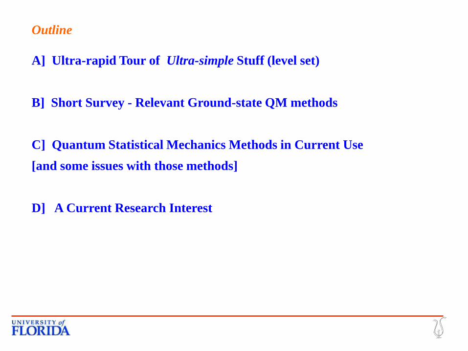
A] Ultra-rapid Tour of Ultra-simple Stuff (level set)

B] Short Survey - Relevant Ground-state QM methods

C] Quantum Statistical Mechanics Methods in Current Use

[and some issues with those methods]

D] A Current Research Interest

Outline

THANKS – BUT NO BLAME – TO

U. Florida Orbital-free DFT Group:

Jim Dufty, Támas Gál, Frank Harris, Valentin Karasiev, Keith

Runge, Travis Sjostrom

Mexican DFT Collaboration:

José Luis Gázquez, Jorge Martín del Campo, Alberto Vela

To Begin

DISCLAIMER: Can’t cover everything in this topic!

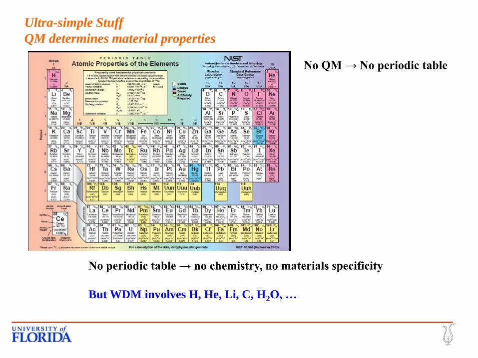
Ultra-simple Stuff

QM determines material properties

No QM → No periodic table

No periodic table → no chemistry, no materials specificity

But WDM involves H, He, Li, C, H2O, …

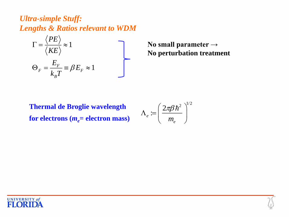
No small parameter →

No perturbation treatment

Ultra-simple Stuff:

Lengths & Ratios relevant to WDM

Thermal de Broglie wavelength

for electrons (me= electron mass)

1/222

:e

em

1

1FF F

B

PE

KE

EE

k T

Ultra-simple Stuff:

Units relevant to WDM

1 Hartree au, magnetic field:

51 2.35 10 TeslaHartreeB

2

1

1 E 27.2116 eV ; 1 bohr = 0.5292 Å

1One-electron KE: r2

e e

Hartree

m q

d

Hartree atomic units

1 Hartree au , pressure:

31E / bohr 294.2Mbar

= 0.2942 Tbar

Hartree

Ultra-simple Stuff

Lengths & Ratios relevant to WDM

Simple cubic H at 1 g/cm3

(≈ 1.8 compression)

Lattice parameter: a = 2.24 au

Te (K) e (au)

100 140.9

104 14.09

105 4.45

106 1.41

a

e(T=105 K) ≈ 2a

Even at T=105 K , the electron is

effectively about twice the size of the

cube edge! QM for the electrons is

unavoidable.

Ultra-simple Stuff

Simplest QM models – H atom

Basic H atom eqns:

panda.unm.edu/Courses/Finley/P262/Hydrogen/WaveFcns.html

2

2

22 1

1

fine structure corrections;

1 1ˆ2

11,2,

2

2 2( , )

nlm nlm nlm nlm

nlm

lr

l mnnlm nl n l l

Hr

nn

r rc e L Y

n n

Paradigm for spectroscopy

Note: vacuum boundary conditions

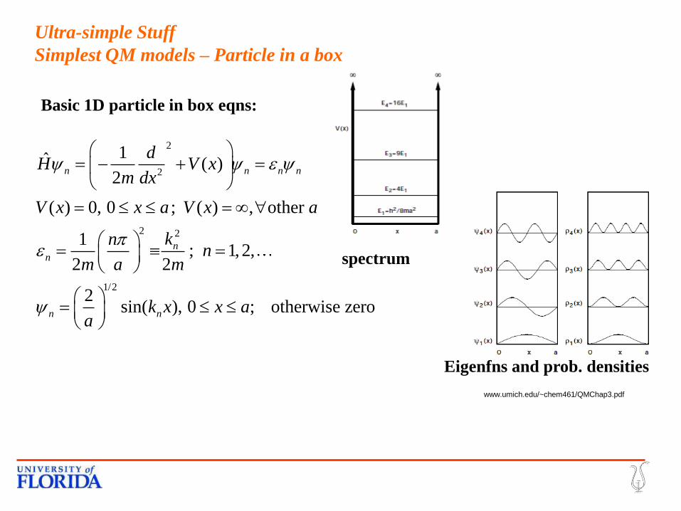
Ultra-simple Stuff

Simplest QM models – Particle in a box

Basic 1D particle in box eqns:

www.umich.edu/~chem461/QMChap3.pdf

Eigenfns and prob. densities

spectrum

2

2

2 2

1/2

1ˆ ( )2

( ) 0, 0 ; ( ) , other

1; 1,2,

2 2

2sin( ), 0 ; otherwise zero

n n n n

nn

n n

dH V x

m dx

V x x a V x a

knn

m a m

k x x aa

Ultra-simple Stuff

Simplest QM models – Homogeneous Electron Gas

HEG eqns:

Uniformly

smeared electrons

Uniformly

smeared nuclei

+

2 211 1 2

1 1 2

1/3

2 2 1/3 1/3

2

Non-interacting case (energy per electron)

Include exchange (energy per electron)

( )1 1 1 1 1ˆ R2 2 2

3 9 1; : (3 )

10 4

1.105 0.458E

i

i i j i j

F F

s

s

nH n d d n d d

E k k nr

r r

r

r r rr R r rr r

2

Also include correlation (energy per electron)

for small1.105 0.458

E 0.048 ( )

s

s s

s s

O r rr r

1/3

1/33:

4sr n

n

Born-Oppenheimer MD – ion forces

from gradient w/r ion coordinates of

ground state “potential surface”

Many-electron Hamiltonian and Born-Oppenheimer Approximation

0;,

1

2

NJ K

I I

J K J K

Z Z

R

FR R

Born-Oppenheimer Approximation: Ne-electrons in the field of

N nuclei at positions {R}

1 1

2

1 ,

,21 1

2 21

1 ,

1 1

1 1 1 1 1;

ˆ ˆ ˆ( , , ) ( ) ,

1 1ˆ2 2

1ˆ ,

ˆ ˆ: , ; ,

ˆ , , , , ; , , ,

e e

I

e e e

e

e e

e e e e

N NN N

N NI J

NN

I I JN I J

N N N N

IN i

i i j i I i Ii j

N ext Ne

N j N N j Nj

Z Z

m

Z

V

R

R

R

R

R R

R r r R r r

RR R

r rr Rr r

r r R r r

r r r r R r r ;eN R

2,2

2 1 1

1 2

*

2 2 2 2

, 2 1 1 1 1

1 1 2

2

,,

( )1, ;

2

, ; , ;, ; , ;

( ) , ;

i j

HF RI

I i I

Ni

m m i j

i

n

iHF Ri

j

j

j

n rZdr r R

r rr R

r R r Rdr r R r R

r r

n r r R

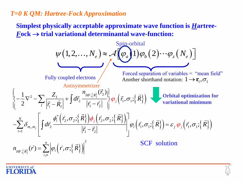
Simplest physically acceptable approximate wave function is Hartree-

Fock trial variational determinantal wave-function:

1,2, , 1 2e a b z eN N

Forced separation of variables = “mean field” Fully coupled electrons

Orbital optimization for

variational minimum

Spin-orbital

SCF solution

Another shorthand notation: 1 11 , rAntisymmetrizer

T=0 K QM: Hartree-Fock Approximation

T=0 K QM: Hartree-Fock Interpretation & Koopmans’ theorem

1:e eN N HOMOI E E

The Ionization Potential (energy to remove least-bound electron to

infinity) is approximately related to the HF eigenvalue spectrum by:

HF characteristic – “HOMO-LUMO” gap

usually overestimates the fundamental gap A= electron affinity

“HOMO” = highest occupied molecular orbital = the highest

occupied HF one-particle energy level.

This result is approximate because it assumes

a) “frozen orbitals” – the one-particle states of the ionized system are the

same as in the ground state

b) the validity of the single-determinant wave function (no correlation)

gap I A

Anticipatory warning: Koopmans’ theorem does not hold for

Kohn-Sham DFT eigenvalues.

HLgap HighestOccupiedMolecularOrbital LowestUnoccMolecularOrbital

CI is not the same as an ensemble average

0

1

2

1 1

ψ 1,2, , : (1 )

1 2

2

1

1 2

2

1

2

e

e

CI e j j e

a b z e

b z e

a z e

N a

A

B

b

zA e

Z

BN

e

N c D N

c N

c N

c N

c N

Nc

“excited” Slater

determinants

T=0 K QM: Configuration Interaction

1

* * *

0 1 1ˆ

e etrial CI CI N j k j k Nd d c c D D d d

r r r r

CI is a linear combination of singly, doubly, triply, etc. “excited”

determinants with the coefficients determined variationally :

Phase relationships between determinants Dj enter in expectation

values, e.g. the variational total energy:

• CI is computationally expensive.

• Picking truncations of it can lead to anomalies (size consistency

problems). There is a cottage industry of “active space” methods for this.

• A variational trial function which is a sum of several configurations and

optimized orbitals can be useful. This is “multi-configuration self-

consistent field”. A trivial 3-term example would be

• The MCSCF Euler equation looks like HF with many more orbitals.

• The physics is in picking which orbital types (symmetries) to include.

• For WDM, this scheme is most relevant to computing accurate T=0 K

atomic spectra. [Example: S.B. Hansen et al. , High En. Dens. Phys. 3, 109

(2007), which uses Gu’s FAC code; see Can. J. Phys. 86, 675 (2008)]

1

1

1

ψ 1,2, , [ (1) ( )]

[ (1) ( )]

[ (1) ( )]

Ne

Ne

Ne

MCSCF e A A A A e

B B B B e

C C C C e

N c D N

c D N

c D N

T=0 K QM: Multi-Configuration SCF

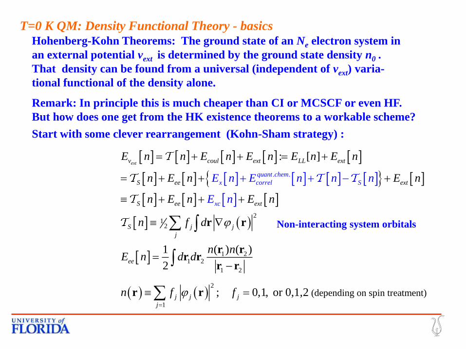
Remark: In principle this is much cheaper than CI or MCSCF or even HF.

But how does one get from the HK existence theorems to a workable scheme?

T=0 K QM: Density Functional Theory - basics

21

2

1 21 2

1 2

2

1

. .

(depending on spin tr

: [ ]

( ) ( )1

2

; 0,1, or 0,1,2

extv coul ext LL ext

S ee ext

S ee ext

quant chem

x corr

S j j

j

ee

j j

l

x

j

e

c

j

S

E n n E n

E n E n n n

E n E n E n

n E n E n

n E n E n

n f d

n nE

E n

n d d

n f f

r r

r rr r

r r

r r eatment)

Hohenberg-Kohn Theorems: The ground state of an Ne electron system in

an external potential vext is determined by the ground state density n0 .

That density can be found from a universal (independent of vext) varia-

tional functional of the density alone.

Start with some clever rearrangement (Kohn-Sham strategy) :

Non-interacting system orbitals

Original system’s

Euler equation:

/

0

ee

xcLL S ee

LL ext e

See ext

xc

v d n

E nE n n E n

E n d n v d n N

v vn

E

n

r r r r r

r r r r r

r rr r

[ ] [ ]KS S KS

SKS

E n n d n v

vn

r r r

rr

Comparison gives

KS ee exx

tcE

v v vn

r r r

r

T=0 K QM: Density Functional Theory – KS eqns

2

2

1

;KS j j j j j

j

v n n

r r r

And the famous KS eqns are:

For a non-interacting system (KS system) with the same density and

T=0 K QM: DFT – some relevant facts

The KS eigenvalues obey the

Slater- Janak thm (not Koopmans’) - KS

jj

En

HLgap HighestOccupiedMolecularOrbital LowestUnoccMolecularOrbital

usually is a poor approximation (30-50% too small) to the fundamental gap, I-A.

Explicit approx. Exc functionals (Local density approx., Generalized gradient

approx., meta-GGAs) either do not correct for self-spurious self-repulsion at all or

inadequately. The IP Theorem is not satisfied and “HOMO-LUMO” gap

HOMOI IP Theorem – For the exact XC functional

T=0 K QM: DFT– more relevant facts

Moreover, the KS orbitals are constrained to construct the density and

minimize the KE operator expectation. They also define the DFT exchange energy.

That’s all (But see Görling-Levy pert. theory.)

DFT details: Tutorial week lectures by Kieron Burke and SBT; talks this

week by H. Gross, K. Burke, S. Pittalis, A. Mattsson

2

1

,

2

2

,

ˆ

( )

ˆ( )

j k

j k j k

j k j k

j k

OK

K O

A related consequence is that eigenvalue differences from such functionals used

in many-body expressions typically are too small.

Schematically:

( ) ( )( )1

0

( ) ( ) ( )

( )one element of complete set fermion states

( ) ( ) ln Tr

( ) : ( ) ; 1/ ( )

:Tr

e

ee e

e

e

e

e

d nN

N

ex

N N

i i

i

N

i

t B

N

N

p V e

v k T

A A

r r r

r r

∣ ∣

Quantum Statistical Mechanics - intro

Grand canonical ensemble

Features to notice:

1] Variational principle goes from to .

2] Often this correspondence is a good heuristic for thinking about finite T

expressions in terms of something familiar at T = 0 K.

3] The boundary conditions on i in the Tr are not stated but are essential to the

description of any problem.

4] In the grand ensemble, the particle number Ne is the average determined by

5 ] Unlike CI or MCSCF, phase relations between states don’t enter in ensembles

O ˆTrO

ˆ ; 1i i i i

i i

O w O w

Many-electron Free-energy in field of nuclei fixed at {R}

Quantum Stat. Mech. : finite-T BOMD

1

( , )2

NI J

K K

I J I J

Z ZT

F R

R R

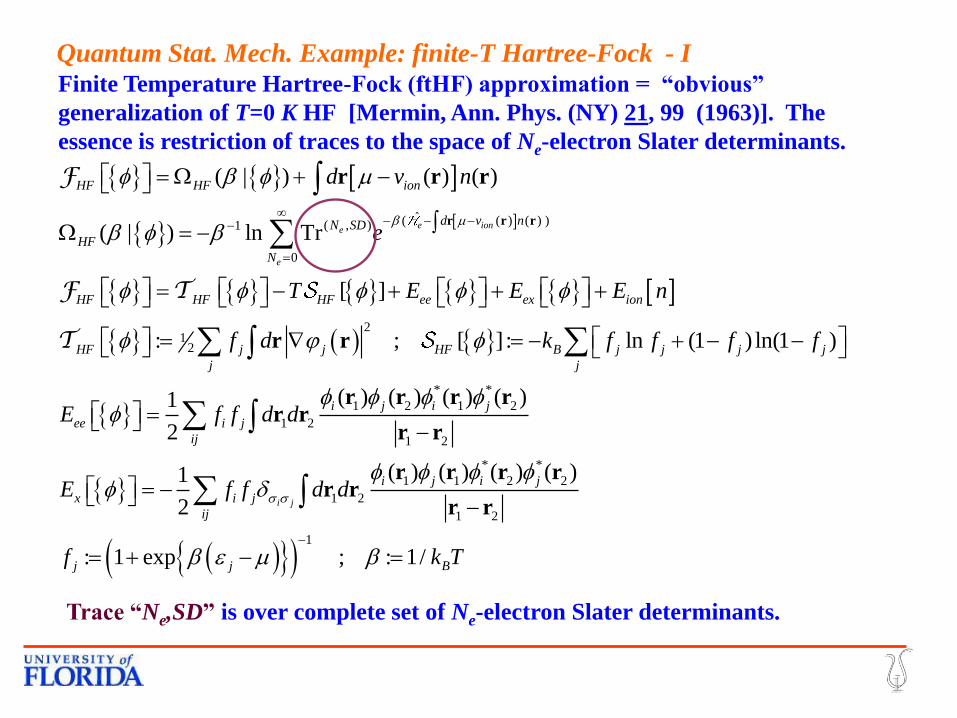
Trace “Ne,SD” is over complete set of Ne-electron Slater determinants.

ˆ( ( ) ( ) )( , )1

0

21

2

( | ) ( ) ( )

( | ) ln Tr

[ ]

: ; [ ] : ln (1 ) ln(1 )

e ione

e

HF HF ion

d v nN SD

HF

N

HF HF HF ee ex ion

HF j j HF B j j j j

j

d v n

e

T E E E n

f d k f f f f

r r r

r r r

r r

F

F T

T

* *

1 2 1 2

1 2

1 2

* *

1 1 2 2

1 2

1 2

1

( ) ( ) ( ) ( )1

2

( ) ( ) ( ) ( )1

2

: 1 exp ; : 1/

i j

j

i j i j

ee i j

ij

i j i j

x i j

ij

j j B

E f f d d

E f f d d

f k T

r r r rr r

r r

r r r rr r

r r

Finite Temperature Hartree-Fock (ftHF) approximation = “obvious”

generalization of T=0 K HF [Mermin, Ann. Phys. (NY) 21, 99 (1963)]. The

essence is restriction of traces to the space of Ne-electron Slater determinants.

Quantum Stat. Mech. Example: finite-T Hartree-Fock - I

*

2 22

2

2

*

2 2

2

2

1

2

( ) ( )( ) ( ) ( ) ( )

( ) ( )( )

i j

j j

i ion

j

ji i

j

j

j

i

i

j

v d

d

f

f

r rr r r r r

r r

r rr r

r r

=

Variational extremalization expected generalization of the T=0 K

HF equation:

Quantum Stat. Mech. Example: finite-T Hartree-Fock - II

1 21

2

1

. .

2

[ ]

[ ]

: [ ]

: 1 e

[ ] [

p

]

x

ionv coul ion e ion ion

S s ee ion e ion ion

S s ee i

quant chem

x c

on e ion ion

S j j

j

j j

orrel S s

xc

E n E n n

n n E n E n T n E

n T n E n E n E

n T n E n E n E

n d

f

n n n

n

d

T

r r

r r

F T

T

T

T

T

T

F

2

1 21 2

1 2

1 2 2

( ) ( )1

2

( ) ( )

: 1 exp

j

ee

ion e ion e

j j j j

j j

n nE n d d

E n d n v

n f

r rr r

r r

r r r

r r r

Again: notice close parallel

with T = 0 K theory, here DFT

Quantum Stat. Mech.: finite-T DFT - I

Mermin [Phys. Rev. 137, A1441 (1965)]; in Hartree au as usual

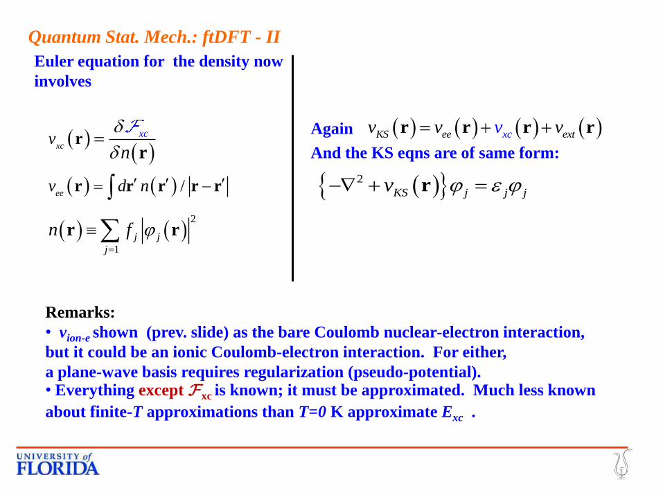
Euler equation for the density now

involves

2

1

/

xc

ee

j j

j

xcv

v d n

n

n f

r

r r r r r

r

r r

Again KS ee exx tcvv v v r r r r

Quantum Stat. Mech.: ftDFT - II

2

KS j j jv r

And the KS eqns are of same form:

Remarks:

• vion-e shown (prev. slide) as the bare Coulomb nuclear-electron interaction,

but it could be an ionic Coulomb-electron interaction. For either,

a plane-wave basis requires regularization (pseudo-potential). • Everything except Fxc is known; it must be approximated. Much less known

about finite-T approximations than T=0 K approximate Exc .

ˆ( ( ) ( ) )( , )1

0

. .

21

2

( | ) ln Tr

[ ] [ ] [ ] [ ] [ ]

[ ] [ ] [ ]

[ ] : ; [ ] :

e ione

e

d v nN SD

EXX

N

EXX S S ee x ion c

quant chem

c correl S s

s j j s

j

e

n n T n E n E n E n E

E E n n n T n n

n f d n

r r r

r r

F T

T T

T

* *

1 1 2 2

1 2

* *

1 2 1 2

1 2

2

1

1

2

ln (1 ) ln(1 )

( ) ( ) ( ) (

( ) ( ) ( ) ( )

)1

2

1

2 i j

B j j j j

j

i j i j

ee i j

ij

i j i j

x i j

ij

k f

E f f d d

f f f

E f f d d

r r r r

r r r rr r

r r

r rr r

A. Görling’s talk

Quantum Stat. Mech. Example: finite-T , Exact-exchange DFT

Finite-T exact-exchange Density Functional Theory in the Kohn-Sham

context has the same structure as ft-HF UNTIL the variational minimization.

x

xvE

n

r

rM. Greiner, P. Carrier, and A. Görling,

Phys. Rev. B 81, 155119 (2010)

A. Görling., J. Chem. Phys. 123, 062203(2005)

EXX has a LOCAL Kohn-Sham

potential, NOT the HF non-local X potential:

This method was in Predrag Krstić’s Workshop II talk about the

plasma-material interface. Usually the method is presented at T=0 K

but nothing prevents doing ftDFT as shown here.

Quantum Stat. Mech. Self-consistent Charge Tight-binding DFT

M. Elstner et al.Phys. Rev. B 58, 7260 (1998)

M. Elstner et al., J. Comput. Chem. 24, 565 (2003)

Suppose a reasonable reference density n0(r) such that the actual density is a

small perturbation: n = n0 + δn. Furthermore, assume that only valence

density variations are significant. Expand the DFT energy in powers of δn.

2/2

12,0 1 2 1 2

1 2 0

1 2,0 ,01

2 1 2 ,0 ,0 ,0

1 2

1,0212,0 1 ,0

1

1ˆ( ) ( ) ( )

( ) ( )[ ] [ ]

( )ˆ [ ]

nxc

i i KS i

i

xc xc core

IKS xc

I I

f h d d n r n rn n

n nd d n d n v n

nZh d v n

R R

R R

R R R

R

R

R r rr r

r rr r r r r

r r

rr r

r R r r

Then come several semi-empirical procedures well-known in solid-state electronic

structure and quantum chemistry. Summary on next slide.

Essence of semi-empirical quantum chemistry and solid-state tight-binding schemes is to

build the Hamiltonian matrix in a basis WITHOUT evaluating the matrix elements as

explicit multi-dimensional integrals.

SCC-TBDFT semi-empirical procedures have some twists: a localized minimal basis,

neglect of 3,4-center matrix elements, and parameterization of the remaining matrix

elements.

,0 ,0

,

0, 0 0

0,

0

basis of localized (Eschrig) atomic eigenfunctions

atomic eigenvalues;

Mulliken population, atom

ˆ ˆ [ ] [ ]

; atomic-sitecharges

KS KS

i i

A B

A KS KS B

I I I I I

I

I I

b

h h T V n V n

n n n q q q

q

q

,

2

0

number of valence electrons on in ref. config.

; both from atomic prescriptions

I

xcAB AA

I

n n

Quantum Stat. Mech. Self-consistent Charge Tight-binding DFT - II

/2

12,0

,

,

ˆ({ }) ({ })

1({ })

2

n

SCTB i KS i IJ I J rep

i I J

NJ K

I I SCTB

J K J K

h q q

Z Z

R R

RFR R

• Single nucleus, charge Z, at origin.

• “Muffin –tin” potential and charge density inside

sphere radius R (“C” in fig.).

• Charge neutrality inside sphere determines R.

• Jelium positive charge outside determines plasma

density (“B” in fig.), which is modeled with HEG

and matched to charge neutrality outside R (“D” in

fig.). Ion distribution

• T= 0 K LDA for X (no C)

• Dirac KS eqns inside sphere with finite-T Fermi-

Dirac occupations.

• Procedure for handling continuum states.

• Two prescriptions for (“T”, “A”) for separating

atomic contributions.

• Prescription for interpolating to TFD at high T

(107 K); this does not seem to be published.

Average Atom – Liberman’s scheme

Kohn-Sham local density

eignvalues for spectra?

Ion radial distribution

averaged away? (Ion-Ion

interactions are gone.)

INFERNO: D.A. Liberman, Phys. Rev. B 20, 4981 (1979)

PURGATORIO: B. Wilson et al. J. Quant. Spectrosc. Rad. Transf. 99, 658 (2006)

PARADISIO M. Pénicaud, J. Phys. Cond. Matt. 21, 095409 (2009)

( ) ( )G r r R

B. Wilson’s talk?

Does the truncated cluster

expansion retain variational

property?

Ion radial distribution

averaged away? (Ion-Ion

interactions are gone.)

R. Piron, T. Blenski, and B. Cichocki, J. Phys. A Math. Theor. 42, 214059 (2009)

R. Piron and T. Blenski, Phys. Rev. E 83, 026403 (2011)

Variational Average Atom – Piron, Blenski, & Cichocki

• Single nucleus, charge Z, at origin.

• Charge neutrality inside sphere determines R.

• Ion distribution

• Free energy expansion w/r reference jelium n0

terminated at first-order

•Use this as a variational expression with n0 to be

determined self-consistently. • ΔF1 is shift of free energy of ion with respect to

jelium – akin to an INFERNO-like shift • Finite-T DFT (with Dirac-Kohn-Sham) for ΔF1

• XC=LDA, finite-T Perrot 1979, Ichimaru at al.

1987

• Virial pressure

( ) ( )G r r R

1 3(3 / 4 )iR n

0 0 0 1 0[ | , , ] [ , , ] [ | , , ]I I In n n n n n n n

• Functional derivatives are closely related to “direct correlation functions”

• Satisfy quantum Ornstein-Zernike equations.

Talk by D. Saumon

Variational Average Atom with Radial Ion-Ion Correlations

C.E. Starrett and D. Saumon, Phys. Rev. E 85, 026403 (2012)

0 0

2

1 2 1 2

1 2 0

2

1 2 1 2 1 2 1

1 2 0

[ , ] [ , ] [ , ]

( ) ( ) ( ) ( )( ) ( )

1 1( ) ( ) ( )

2 ( ) ( ) 2

ext extI e

ext extI e

exc exc exc

e I e I e I

excexc exc

e e I I e I

e I V V

exc

I I e e

I I V V

n n n n n n

d n d n d d n nn n

d d n n d d n nn n

r r r r r r r rr r

r r r r r r rr r

2

2

1 2 0

( )( ) ( ) ext ext

I e

exc

e e V Vn n

rr r

• Single nucleus, charge Z, at origin

• Ion distribution outside is included in spherically averaged sense.

• Ion distribution constructed consistently with nucleus-centered problem

• Uses DFT for ions and electrons

• Truncates “excess” free energy (non-ideal contribution) at second-order

in functional Taylor expansion around reference densities -

Calibration of Approximate Functionals? PIMC

which has a non-negative integrand – good for MC sampling. Fermion anti-

symmetry still to be imposed. D. Ceperley’s talk.

“Computational Methods for Correlated Systems, Lecture 3”

http://www.phys.ufl.edu/courses/phy7097-cmt/fall08/lectures/index.html

“Path Integral Monte Carlo” B. Bernu and D.M. Ceperley

http://www2.fz-juelich.de/nic-series/volume10/volume10.html

Factorization

to paths

2

1

(3 /2)0 1 11

( )1, ; exp ( )

(4 ) 4e

MM M

N MM M Me e

d d V

r rr r r r r

Despite the fact that KE and PE operators don’t commute

This allows separation of KE and PE contributions

ˆˆ ˆexp( ) lim exp[ ( / ) ( / ) ]M

MM M V

*

0 1 1 0 1 1

, ; exp( )

ˆ

ˆ ˆ ˆexp( ) exp[ ( / ) ] : exp( )

, ; , ; , ;

i i i

i

i i i

MM

M M M M

E

E

M

d d

r r r r

r r r r r r r r

ftDFT in practice today Typically one of two flavors

o BOMD with a code such as VASP and Fxc[n(T), T] Exc[n(T)]

o Some form of Thomas-Fermi + von Weizsäcker for KE (discussion

below about orbital-free schemes)

Talks by Ronald Redmer, Joel Kress, Flavien Lambert, (others ?)

Q: Is a ground state functional with implicit T-dependence good enough?

Talk by Travis Sjostrom

Many-body transport coefficients calculated with Kohn-Sham inputs.

Example: Kubo-Greenwood electrical conductivity:

2

,

2

3i j i j i j

i j

w

f fV

k k

k BZ

k k k k k k k

Remark: In principle, this is a misuse of the KS orbitals and eigenvalues.

Q: How good (bad) an approximation is it to do that?

Q: What can be done to characterize (and, one hopes, bound) the errors

from doing that?

o Discussion of coupled-cluster methods omitted from T=0 K QM survey for

brevity. For small molecules, these generally are accepted as the “gold

standard” for calibration and validation of other methods (in some aspects better

than experiment).

o Omitted quantum statistical potentials, wave packet MD, PIMD, DFT

embedding, QM Green’s fns, hybrid functionals, range separation, time-dep.

DFT, …

o The literature for quantum stat. mech. relevant to WDM is scattered in

maddeningly many disparate journals: Phys. Rev. A, B, E; Phys. Rev. Lett.; J.

Chem. Phys.; J. Phys. Cond. Matt.; J. Phys. A; J. Phys. Chem.; J Chem. Th.

Computation; Phys. Plasmas; High En. Dens. Phys.; Contrib. Plasma Phys.; J.

Quant. Spectr. Rad. Transf.; Comput. Phys. Commun.; Phys. Chem. Liq.; J.

Non-Cryst. Solids; Theoret. Chem. Accounts; … etc.

o Plasma community makes assumptions about the readership which are at odds

with the diversity of backgrounds from which folks come to WDM.

o Conversely, the jargon of many-body and cond. matter physics can be difficult

and the jargon of quantum chemistry is far more so.

o Despite convenient language, BOMD with quantum stat. mech. electronic forces

is not “quantum MD”.

Quantum Stat. Mech. for WDM – Miscellaneous Remarks

Orbital-free DFT – Aspects of Approximate Functional Development

OFDFT MOTIVATION -

A personal fascination

A potentially enormous boost to WDM simulations The K-S decomposition is valuable: it provides a one-

body system that gives the physical density and free energy.

But the K-S orbital structure is

o expensive computationally

o not essential conceptually

[ , ]

( )[ ( )]

[ , ] [ ( ), ]

[ ( ), ]s B

s sKS

s S

Sn T k

Tv n

n

n T d t n T

d s n T

r

r r

r r

T

T

Constraint-based Orbital-free finite-temperature DFT (“of-ftDFT”)

of-ftDFT is back to basics:

exact at T= 0 K and

finite T [PRB 84, 125118 (2011)] [ ] [ ] [ ], [ ] 0s Wn n n n

2

0

1(r) (r) (r) (r)

2

(r) ( ) , lim 0 r

KS

sT

v v n n

v T n v

Then given Fxc , the of-ftDT Euler equation is

2( )1

:8

W

nn d

n

rr

r

Four challenges – a) Non-interacting Fs has two contributions: KE and entropy

b) Fxc has two contributions: X, C

Task – design functionals which respect as many known results (limits,

bounds, asymptotics, etc.) as possible.

Remarks:

a) Frequent criticism of T=0 K KS-DFT is “there is no systematic way

to improve the XC functionals”. A more accurate remark is that

there is no mechanical recipe to add complexity to XC functionals.

b) Added complexity is not a guarantee of improved accuracy

c) There is a horrendous amount of empiricism, fiddling, and

combining of bits and pieces of functionals to achieve “successful”

error cancellation (mostly in quantum chemistry). Most of this can

be ignored beneficially.

d) But some empirical functionals are useful for showing how much can

be achieved with a given level of complexity or refinement.

Adventures in Constraint-based functional development

Sam’s Excellent Adventures in Functional Design

Credit: Bobby Scurlock

¡Adelante!

T= 0 K X , Lieb-Oxford Bound, and Generalized Gradient Approximations

, 1/3[ , ] 1.804

2

LOx GGAF n s

Satisfaction of the L-O bound for all possible spin densities n (r), and

all inhomogeneity values s(r) imposed as a sufficient condition -

,

1/3

4/3

; 2.275 ( 2.2149)

3 3( ) , :

4

LDA

xc LO x LO LO CH

LDA

x x x

E E

E c d n c

r r

Constraint on construction

of XC functionals E. Lieb and S. Oxford, Int. J. Quantum

Chem. 19, 427 (1981); J.P. Perdew in

“Electronic Struct. Of Solids ’91”, 11 (1991);

G. Chan and N. Handy, Phys. Rev. A

59, 3075 (1999)

2 1/3 4/3

4/3

1 | |( ) :

2(3 )

[ ] ( ) ( ( ))x x xGGA

GGA

ns

n

E n c n F s d

r

r r rGeneralized Gradient

Approximation for X

Vela-Medel-Trickey X Enhancement Factor (VMT) -

22

2

1/3

( ) 11

10where GEA (PBEsol) or 0.21951 (PBE)

81

( ) / 2

sVMT

x

VMT

x MAX LO

s eF s

s

F s

4081 81: 120

MAXs

2: 1

1 /

PBE

xFs

J. Chem. Phys. 130, 244103 (2009)

• s 0 : Fx VMT

1 (homogeneous electron gas)

• Lieb-Oxford bound : Fx VMT

≤ 1.804

• Large s limit homogeneous electron gas

Reminder:

Comparison of X Enhancement Factors -

limss1/2FXC Only PW91 X satisfies the large-s constraint

M. Levy & J.P. Perdew, Phys. Rev. B 48, 11638 (1993)

VMT recovers HEG behavior for large-s while staying below

the LO bound for all but one value of s

VT{mn} adds satisfaction of the large-s constraint

FXVMT (s) 1

s2 e s2

1 s2

/2

2

/2

{ }

2/2

/

2

2( ) ( )

1 1 11

1 1m

m

VT mn VMT

X X

s

s

n

n

s

e sF s F s

s ee s

s

VT{84} Exchange

FUNCTIONAL DESIGN: m and n are fixed by:

• m, n must be integers.

• The leading term in the small-s expansion of Fx must be quadratic.

• Rotational invariance only even powers of s are allowed.

• Limit s→0 must = 1 to recover HEG behavior.

m,n = 8,4: αPBE = 0.000069, αGEA = 0.000023

; / 2 and ( ) / 2 areevenm n m m n

J. Chem. Phys. 136, 144115 (2012)

VT{84}(μPBE) = VT{84}

VT{84}(μGEA) = VT{84}sol

PW91

Fx

s

Why 8,4? Design Choices

Larger m,n increasingly make a kink here

No physics in that (Occam’s razor).

Typical Test Sets in this specialty: Raghavachari, Curtiss, Perdew,

Scuseria, Truhlar, Hobza, Cheeseman

• G1 for atomization energies (fixed geometries).

• G3 for standard heats of formation at 298 K (geometry optimizations +

harmonic analysis). Only example presented here.

• Ionization potentials, electron and proton affinities with optimized

geometries.

• Weak interactions.

• Hydrogen and non-hydrogen transfer barrier heights (fixed

geometries).

• Transition metals

• Chemical shifts

• VT{mn} and VMT implemented in development versions of deMon2k

and NWChem.

VT{84} and VMT: Molecular Tests

TPSS PBEsol PBE VMT VT84 VMTsol VT84sol

PBE-C except

TPSS

DZVP 8.22 55.32 20.38 10.87 10.20 48.98 48.58

def2-

TZVPP 5.40 59.63 21.92 11.00 10.42 53.01 52.58

LYP-C except

TPSS

DZVP 8.22 39.55 11.89 7.79 8.14 33.43 33.05

def2-

TZVPP 5.40 43.53 13.04 7.48 7.63 36.97 36.55

G3 Data Set: Mean Absolute Errors for Standard heats of formation at 298 K /

kcal-mol-1 (223 molecules) TPSS is a “meta-GGA”, LYP is a correlation

functional. 1 kcal/mol = 0.043 eV/atom

VT{84} is 53% better than PBE-PBE and 42% with LYP (PBE-

LYP vs. VT{84} –LYP) using a TZVPP basis set

VT{84} and VMT: Molecular Tests

J. Chem. Phys. 136, 144115 (2012)

But that’s only XC

Those benchmark calculations were pure Kohn-Sham -

KS KE without orbitals?

KS entropy without orbitals?

Feed the OF-KE functionals the

density from the KS calculation

(“exact” for these purposes).

Calculate new total energy

vs. bond length for SiO stretch.

OF-DFT at T=0 K: Test of Existing Single-point (GGA) KE functionals

PW91: Lacks and Gordon, J.Chem. Phys. 100, 4446 (1994)

PBE-TW: Tran and Wesolowski, Internat. J. Quantum Chem. 89, 441 (2002) [

GGA-Perdew: Perdew, Phys. Lett. A 165, 79 (1992)

DPK: DePristo and Kress, Phys. Rev. A 35, 438 (1987)

Thakkar: Thakkar, Phys. Rev. A 46, 6920 (1992) SGA: Second order Gradient Approx. TS = TTF + (1/9) TW

J. Comput. Aided Matl. Design 13, 111 (2006)

KS

All six Ts approximations fail to

bind! V violates positivity.

Parameterizations

• Tried two simple forms for modified enhancement factors. These forms would

be convenient for use in MD. No guarantee that any of these is optimal.

21

21

( ) 11

jN

PBE N

t j

j

sF s c

a s

2 21 2exp4

1 2(1 ) (1 )a s a s

tF C e C e

“Conjoint” - Ft Fx

N=2 is typical PBE form; also used by Tran & Weslowski

N=3 is the form used by Adamo & Barone [J. Chem. Phys. 116, 5933 (2002)]

N=4 highest tried

• Constrain parameters to 0v Initial parameterization used

(a) single SiO or

(b) SiO, H4SiO4, and H6Si2O7.

Stretched single Si-O bond in all cases with self-consistent KS densities.

OF-KE at T=0 K: Modified conjoint KE functionals

Single bond stretch

gradient for H2O

(negative of force).

OF-KE parameters

from 3-member

training set (SiO,

H4SiO4, and H6Si2O7)

except PBE2.

NO information

about H2O in the set.

OF-KE at T=0 K – Test of Modified Conjoint, Positive-definite Functionals

All our functionals give too large an equilibrium bond length from input KS density.

PROBLEM: mcGGA Pauli potential vθ singularities at nuclei. TOO positive! Phys. Rev. B 80, 245120 (2009).

No.

Bcc Li lattice constant. mcGGA is our PBE-2, parameterized to

SiO , implemented in modified PROFESS code. GGA=Tran & Wesołowski

Are mcGGA Positive Singularities Fatal?

Details: Valentin Karasiev’s Poster

TF

0

TF

0s [ ] ( ) ( ) ( ) ( ) ( ) ( )

( ) d ( ) / d( , ,T) : ( , )

( )

d ( ) / d( , ,T) : ( , )

( )

/

ftGGA

F

n d n t F s d n t F s

h t t h t ts n n s n n

t

t h t ts n n s n n

t

t T T

r r

Form of new

variables

motivated by 2nd

order gradient

expansion.

New of-ftDFT functionals – non-interacting part

from Perrot’s (1979) analytic fit

Beware one obviously wrong

coefficient (exponent) in that fit.

h

New Finite-T

generalized

gradient

approximation via

new variables.

Details: Valentin Karasiev’s Poster

ftGGA based on Tran-Wesolwski T = 0 K ofKE GGA Int. J. Quantum Chem. 89, 441 (2002)

1 1C =0.2319 , a =0.2748TW TW

First try (known to violate some constraints; satisfies an approximate symmetry)

2KST2 1

2

1

2KST2 1

1

1

2

1

( ) : 11

( ) :

C =2.03087 , a =0.29

1

24

1

4

C sF s

a s

C sF s

a s

New of-ftDFT functionals – non-interacting part

mcGGA “PBE2” with new finite-T

inhomogeneity variables

Parameters fitted at T = 0 K to small training set Phys. Rev. B 80, 245120 (2009)

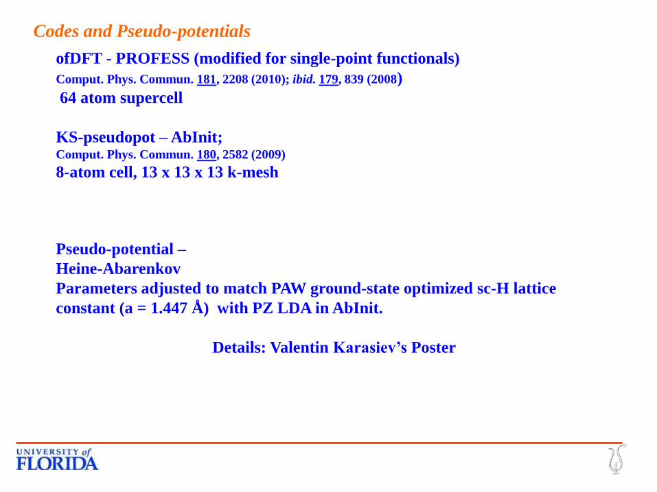
Codes and Pseudo-potentials

Pseudo-potential –

Heine-Abarenkov

Parameters adjusted to match PAW ground-state optimized sc-H lattice

constant (a = 1.447 Å) with PZ LDA in AbInit.

Details: Valentin Karasiev’s Poster

ofDFT - PROFESS (modified for single-point functionals)

Comput. Phys. Commun. 181, 2208 (2010); ibid. 179, 839 (2008)

64 atom supercell

KS-pseudopot – AbInit; Comput. Phys. Commun. 180, 2582 (2009)

8-atom cell, 13 x 13 x 13 k-mesh

Structural Optimization Comparison

Energy per atom vs. material density for sc-H at electronic temperature Te=100 K

(Tion=0 K) for KS and OF-DFT calculations (both with PZ LDA XC functional and

Heine-Abarenkov local pseudo-pot. Nota bene: VW+TF is full VW, ftSGA is VW/9.

P vs. T for five orbital-free functionals and tKS. Simple cubic H, =1.0 g/cm3

(compression 1.8) All with LDA Exc. Includes ion-ion contribution.

sc Hydrogen

T (Kelvin) P(Tpa)

tKS-LDA

P(Tpa)

SGA = tTF +

tvW/9

P(Tpa)

tTF

P(Tpa)

tGGA

KST2

P(Tpa)

tGGA

TW

100 0.1640 0.2463 0.2945 0.1438 0.2631

1000 0.1641 0.2463 0.2946 0.1438 0.2631

10,000 0.1696 0.2502 0.2986 0.1478 0.2669

50,000 0.2754 0.3351 0.3893 0.2393 0.3515

100,000 0.5258 0.5463 0.6094 0.4856 0.5646

scH data for tKS vs of-tDFT

=1.0 g/cm3 (compression 1.8) All with PZ Exc LDA as approximate Fxc .

Includes ion-ion contribution.

Red headings denote failure to give stable ground state.

Finite-T Exchange-correlation free energy

See Travis Sjostrom’s talk for comparison of three T-dependent C functionals.

d f [ , ]xc xcn n T r r r

• “Generalized Gradient Approximation Non-interacting Free Energy Functionals for Orbital-free

Density Functional Calculations”, V.V. Karasiev, T. Sjostrom, and S.B. Trickey, in preparation

• “Issues and Challenges in Orbital-free Density Functional Calculations”, V.V. Karasiev and S.B.

Trickey, Comput. Phys. Commun. [accepted]

• “Comparison of Density Functional Approximations and the Finite-temperature Hartree-Fock

Approximation for Warm Dense Lithium”, V.V. Karasiev, T. Sjostrom, and S.B. Trickey, in

preparation

• “Finite Temperature Scaling, Bounds, and Inequalities for the Noninteracting Density Functionals”,

J.W. Dufty and S. B. Trickey, Phys. Rev. B 84, 125118 (2011)

• “Positivity Constraints and Information-theoretical Kinetic Energy Functionals”, S.B. Trickey, V.V.

Karasiev, and A. Vela, Phys. Rev. B 84, 075146 [7 pp] (2011).

• “Temperature-Dependent Behavior of Confined Many-electron Systems in the Hartree-Fock

Approximation”, T. Sjostrom, F.E. Harris, and S.B. Trickey, Phys. Rev. B 85, 045125 (2012)

• “Constraint-based, Single-point Approximate Kinetic Energy Functionals”, V.V. Karasiev, R.S.

Jones, S.B. Trickey, and F.E. Harris, Phys. Rev. B 80, 245120 (2009)

• “Conditions on the Kohn-Sham Kinetic Energy and Associated Density”, S.B. Trickey, V.V. Karasiev,

and R.S. Jones, Internat. J. Quantum Chem.109, 2943 (2009)

• “Recent Advances in Developing Orbital-free Kinetic Energy Functionals”, V.V. Karasiev, R.S. Jones,

S.B. Trickey, and F.E. Harris, in New Developments in Quantum Chemistry, J.L. Paz and A.J.

Hernández eds. [Research Signposts, 2009] 25-54

• “Born-Oppenheimer Interatomic Forces from Simple, Local Kinetic Energy Density Functionals”,

V.V. Karasiev, S.B. Trickey, and F.E. Harris, J. Computer-Aided Mat. Design, 13, 111-129 (2006)

References – OF-KE and thermal DFT

http://www.qtp.ufl.edu/ofdft