Embed Size (px)
Citation preview

The Recent Shift in Term Structure Behaviorfrom a No-Arbitrage Macro-Finance Perspective¤
Glenn D. Rudebuschy Tao Wuz
October 2004
Abstract
This paper examines a recent shift in the dynamics of the term structure and
interest rate risk. We …rst use standard yield-spread regressions to document such a
shift in the U.S. in the mid-1980s. Over the pre- and post-shift subsamples, we then
estimate dynamic, a¢ne, no-arbitrage models, which exhibit a signi…cant di¤erence
in behavior that can be largely attributed to changes in the pricing of risk associated
with a “level” factor. Finally, we suggest a link between the shift in term structure
behavior and changes in the risk and dynamics of the in‡ation target as perceived
by investors.
¤The views expressed in this paper do not necessarily re‡ect those of the Federal Reserve Bank of San Francisco.yFederal Reserve Bank of San Francisco; www.frbsf.org/economists/grudebusch; [email protected] Reserve Bank of San Francisco; [email protected].
1. Introduction
During the past few decades, the U.S. economy has undergone an important transformation that
has likely altered the nature of uncertainty and risk in the economy as well as investors’ attitudes
and pricing of that risk. A key aspect of this transformation is the precipitous decline in overall
macroeconomic volatility: Since the middle of the 1980s, the volatility of real GDP growth has
been about 35 percent lower than earlier in the postwar period (as noted by Kim and Nelson 1999
and McConnell and Perez-Quiros 2000). Several factors may underlie this “Great Moderation”
in economic ‡uctuations.1 For example, improved economic policies may have helped stabilize
the economy; indeed, many have argued that the conduct of U.S. monetary policy improved
dramatically during the mid-1980s, helping to usher in this period of diminished output volatility
as well as remarkably low and stable in‡ation. Alternatively, the recent quiescence in real activity
and in‡ation may largely re‡ect good luck—that is, a temporary run of smaller economic shocks.
Other potential factors include non-policy changes in the dynamics of the economy arising from,
for example, improved inventory management or a greater share in aggregate output accounted
for by the relatively stable service sector. Finally, the development of deeper and more integrated
…nancial markets may also have played an important role both in damping the magnitude of
economic ‡uctuations and in mitigating their e¤ects on investors. Given such dramatic shifts in
the economic environment, a change in the behavior of the term structure of interest rates, and
especially in the size and dynamics of risk premiums, would hardly be surprising.
This paper examines how the dynamics of the term structure and interest rate risk may have
changed over time. We use a¢ne, no-arbitrage, asset pricing models of the type popular in the
…nance literature to investigate the recent shift in the behavior of the term structure; however,
our investigation is also informed by the above literature on the recent transformation of the
U.S. economy and by consideration of the macroeconomic underpinnings of the term structure
factors in …nance models.2 The payo¤ from this joint analysis is bi-directional as well. The
macro-…nance perspective helps illuminate the nature of the shift in the behavior of the term
structure, highlighting in particular the importance of a shift in investors’ views regarding the
risk associated with the long-term in‡ation goals of the monetary authority. In addition, the1 For references to the quickly growing literature on this topic, see Blanchard and Simon (2001) and Stock and
Watson (2003).2 The connection between the macroeconomic and …nance views of the term structure has been a very fertile
area for recent research, including, for example, Piazzesi (2003), Diebold, Rudebusch, and Aruoba (2004), Hördahl,Tristani, and Vestin (2004), Rudebusch and Wu (2004), Wu (2001), Dewachter and Lyrio (2002), Du¤ee (2004),and Kozicki and Tinsley (2001).
1

shift in term structure behavior, as viewed using a no-arbitrage …nance model, sheds light on
the nature of recent macroeconomic changes. Speci…cally, assuming that the factors underlying
recent changes in macroeconomy have left their imprint on the yield curve as well, the …nance
models suggest that more than just good luck was responsible for the recent macroeconomic
transformation. Instead, a favorable change in economic dynamics, likely linked to a shift in
the monetary policy environment, appears to have been an important element of the Great
Moderation.
We begin our analysis in Section 2 with a simple empirical characterization of the recent shift
in the term structure. For this purpose, we use regressions of the change in a long-term interest
rate on the lagged spread between long and short rates. Following Campbell and Shiller (1991),
such regressions have been widely used to test the expectations hypothesis of the term structure,
which assumes that the risk or term premiums embedded in long rates are constant. We …nd—as
have many others—that these tests often reject the expectations hypothesis; however, of more
interest for our purposes is the apparent signi…cant shift in the estimated coe¢cients from these
regressions. Indeed, since the mid-1980s in the U.S., there is much less evidence against the
expectations hypothesis than before, which suggests a shift in risk pricing and in the properties
of risk premiums.
We use these term structure regression results as a summary statistic for characterizing
the changing empirical behavior of the term structure. Accordingly, the regression evidence
is a useful …rst step to a more formal modeling perspective on the term structure change,
which is provided in Section 3 using an estimated dynamic, a¢ne, no-arbitrage model of bond
pricing. The no-arbitrage model provides an obvious setting in which to examine changes in
interest rate behavior and time-varying term premiums. Indeed, as demonstrated by Backus
et al. (2001), Du¤ee (2002), and Dai and Singleton (2002), a¢ne, no-arbitrage models with
a rich speci…cation of the dynamics of risk premiums are broadly consistent with the usual
full-sample term structure regression results of the type obtained in Section 2. We conduct
a similar consistency check between models and regression results, though from a somewhat
di¤erent perspective. Namely, given our evidence of a signi…cant shift in the term structure
regression results, we estimate a¢ne, no-arbitrage models for each of the two subsamples that
are associated with the di¤erent regression results. We …nd a statistically signi…cant di¤erence
between the two estimated bond pricing models. In addition, the subsample models are able to
2

account for much of the disparity between the subsample term structure regression results, thus
supporting the empirical characterization of structural change in Section 2.
Beyond merely documenting the recent change in term structure behavior through regression
analysis and model estimates, we also consider the more di¢cult task of understanding and
accounting for such time variation. In Sections 4 and 5, we illuminate the economic changes
that may account for the shift in term structure behavior. We …rst use the estimated subsample
no-arbitrage models to parse out whether a shift in the dynamics of risk or a shift in the
pricing of that risk is likely the most important factor accounting for the shift in term structure
behavior. We …nd that changes in the pricing of risk associated with a “level” factor are crucial
determinants of the change in term structure behavior. We then try to provide an interpretation
of this shift in terms of possible recent macroeconomic changes. For this purpose, we employ the
macro-…nance model of Rudebusch and Wu (2004) and link the recent shift in term structure
behavior to changes in the risk and dynamics of the long-run in‡ation target as perceived by
investors.
At this point, it is perhaps useful to discuss other recent related research. There has been
little analysis of the e¤ects on asset pricing induced by the important structural shifts in the
economy documented in the macroeconomics literature and cited above. Indeed, the …nance
literature often treats the entire postwar period as a long homogenous sample. An exception to
this standard practice is the literature on regime-switching models of interest rates, including,
for example, Hamilton (1988), Gray (1996), Ang and Bekaert (2002), Bansal and Zhou (2002),
and Dai, Singleton, and Yang (2003). These papers attempt to capture the postwar dynamics of
interest rates with models that contain a succession of alternating regimes that are often linked
informally to business cycles or interest rate policies. In contrast, we are interested in a single
break in the behavior of the term structure, with our attention focused by the macroeconomic
evidence that suggests the shift occurred during the middle to late 1980s. Also, we have no
expectation that this change will be reversed (and we incorporate no pricing of further regime
change risk). Of course, regime switching at a cyclical frequency could coexist with a single large
shift in risk pricing as well, but our interest is primarily in the latter. Accordingly, our analysis
is related to other work, including Watson (1999), who examined a shift in the unconditional
volatility of interest rates, and Lange, Sack, and Whitesell (2003), who considered a change
in the forecastability of short-term interest rates. However, in contrast to these analyses, we
3
examine a shift in behavior of risk pricing using both simple regression indicators as well as
formal dynamic bond pricing models.
2. Regression Evidence of a Term Structure Shift
In order to help guide our subsequent model-based analysis, we provide in this section a simple
empirical characterization of the recent shift in the behavior of the term structure. Our metric
to assess this shift is based on a regression test of the expectations hypothesis popularized by
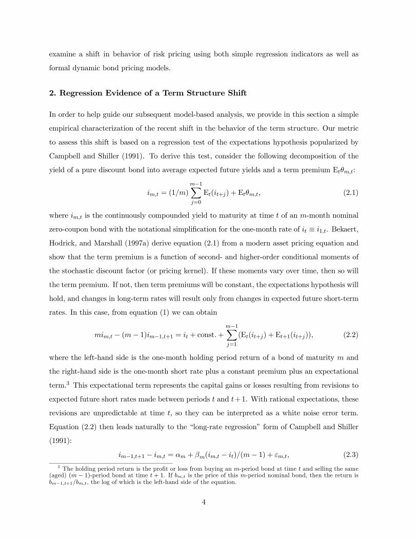
Campbell and Shiller (1991). To derive this test, consider the following decomposition of the
yield of a pure discount bond into average expected future yields and a term premium Etθm,t:
im,t = (1/m)m¡1X
j=0
Et(it+j) + Etθm,t, (2.1)
where im,t is the continuously compounded yield to maturity at time t of an m-month nominal
zero-coupon bond with the notational simpli…cation for the one-month rate of it ´ i1,t. Bekaert,
Hodrick, and Marshall (1997a) derive equation (2.1) from a modern asset pricing equation and
show that the term premium is a function of second- and higher-order conditional moments of
the stochastic discount factor (or pricing kernel). If these moments vary over time, then so will
the term premium. If not, then term premiums will be constant, the expectations hypothesis will
hold, and changes in long-term rates will result only from changes in expected future short-term
rates. In this case, from equation (1) we can obtain
mim,t ¡ (m ¡ 1)im¡1,t+1 = it + const. +m¡1X
j=1
(Et(it+j) + Et+1(it+j)), (2.2)
where the left-hand side is the one-month holding period return of a bond of maturity m and
the right-hand side is the one-month short rate plus a constant premium plus an expectational
term.3 This expectational term represents the capital gains or losses resulting from revisions to
expected future short rates made between periods t and t+1. With rational expectations, these
revisions are unpredictable at time t, so they can be interpreted as a white noise error term.
Equation (2.2) then leads naturally to the “long-rate regression” form of Campbell and Shiller
(1991):
im¡1,t+1 ¡ im,t = αm + βm(im,t ¡ it)/(m ¡ 1) + εm,t, (2.3)3 The holding period return is the pro…t or loss from buying an m-period bond at time t and selling the same
(aged) (m ¡ 1)-period bond at time t + 1. If bm,t is the price of this m-period nominal bond, then the return isbm¡1,t+1/bm,t, the log of which is the left-hand side of the equation.
4
where αm and βm are maturity-speci…c regression intercept and slope coe¢cients, and εm,t is
the white noise expectational term (scaled by 1 ¡ m). Under the expectations hypothesis, the
estimated slope coe¢cient βm will equal unity; that is, the term spread will be an optimal
forecast of future change in the long rate (adjusted for a constant risk premium), so when the
spread between long and short rates widens (narrows), the long rate should rise (fall) in the
following period.
Deviations from the expectation hypothesis will push the slope coe¢cient away from one.
In particular, as noted early on by Mankiw and Miron (1986), a time-varying term premium
can drive the estimated βm to zero or even to negative values as the resulting term spread
re‡ects variation in expected risk premiums rather than in future rates. In our analysis be-
low, we construct models in which the time variation in the term premium (or equivalently the
conditional heteroskedasticity of the discount factor) is su¢cient to generate the regression co-
e¢cients found in the data. Accordingly, we are not primarily interested in the slope coe¢cients
as indicators of the expectations hypothesis; instead, we use them as simple summary statistics
of term structure behavior, and we interpret shifts in these coe¢cients as indications that the
term structure behavior has changed. Of course, the fact that so many researchers have focused
so much e¤ort on estimating these slope coe¢cients makes them of particular interest, but other
simple metrics of term structure change could also be considered (as in Watson 1999 and Lange,
Sack, and Whitesell 2003).
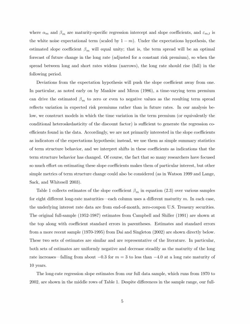
Table 1 collects estimates of the slope coe¢cient βm in equation (2.3) over various samples
for eight di¤erent long-rate maturities—each column uses a di¤erent maturity m. In each case,
the underlying interest rate data are from end-of-month, zero-coupon U.S. Treasury securities.
The original full-sample (1952-1987) estimates from Campbell and Shiller (1991) are shown at
the top along with coe¢cient standard errors in parentheses. Estimates and standard errors
from a more recent sample (1970-1995) from Dai and Singleton (2002) are shown directly below.
These two sets of estimates are similar and are representative of the literature. In particular,
both sets of estimates are uniformly negative and decrease steadily as the maturity of the long
rate increases—falling from about ¡0.3 for m = 3 to less than ¡4.0 at a long rate maturity of
10 years.
The long-rate regression slope estimates from our full data sample, which runs from 1970 to
2002, are shown in the middle rows of Table 1. Despite di¤erences in the sample range, our full-
5
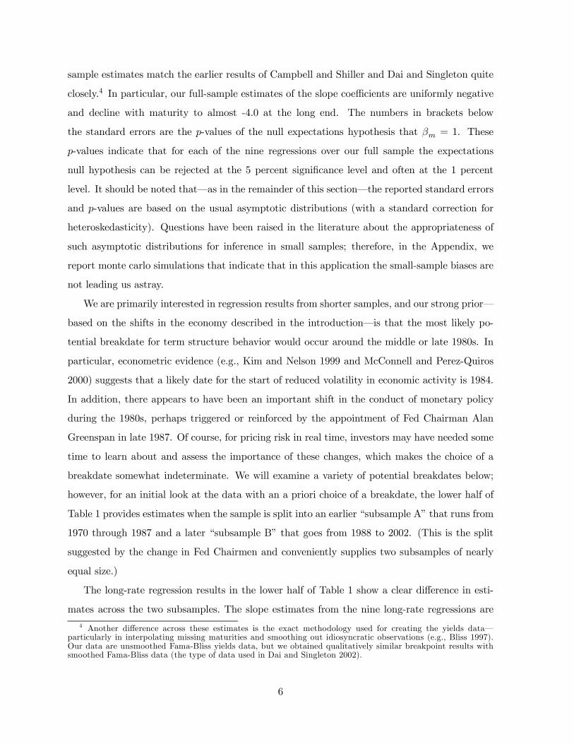
sample estimates match the earlier results of Campbell and Shiller and Dai and Singleton quite
closely.4 In particular, our full-sample estimates of the slope coe¢cients are uniformly negative
and decline with maturity to almost -4.0 at the long end. The numbers in brackets below
the standard errors are the p-values of the null expectations hypothesis that βm = 1. These
p-values indicate that for each of the nine regressions over our full sample the expectations
null hypothesis can be rejected at the 5 percent signi…cance level and often at the 1 percent
level. It should be noted that—as in the remainder of this section—the reported standard errors
and p-values are based on the usual asymptotic distributions (with a standard correction for
heteroskedasticity). Questions have been raised in the literature about the appropriateness of
such asymptotic distributions for inference in small samples; therefore, in the Appendix, we
report monte carlo simulations that indicate that in this application the small-sample biases are
not leading us astray.
We are primarily interested in regression results from shorter samples, and our strong prior—
based on the shifts in the economy described in the introduction—is that the most likely po-
tential breakdate for term structure behavior would occur around the middle or late 1980s. In
particular, econometric evidence (e.g., Kim and Nelson 1999 and McConnell and Perez-Quiros
2000) suggests that a likely date for the start of reduced volatility in economic activity is 1984.
In addition, there appears to have been an important shift in the conduct of monetary policy
during the 1980s, perhaps triggered or reinforced by the appointment of Fed Chairman Alan
Greenspan in late 1987. Of course, for pricing risk in real time, investors may have needed some
time to learn about and assess the importance of these changes, which makes the choice of a
breakdate somewhat indeterminate. We will examine a variety of potential breakdates below;
however, for an initial look at the data with an a priori choice of a breakdate, the lower half of
Table 1 provides estimates when the sample is split into an earlier “subsample A” that runs from
1970 through 1987 and a later “subsample B” that goes from 1988 to 2002. (This is the split
suggested by the change in Fed Chairmen and conveniently supplies two subsamples of nearly
equal size.)
The long-rate regression results in the lower half of Table 1 show a clear di¤erence in esti-
mates across the two subsamples. The slope estimates from the nine long-rate regressions are4 Another di¤erence across these estimates is the exact methodology used for creating the yields data—
particularly in interpolating missing maturities and smoothing out idiosyncratic observations (e.g., Bliss 1997).Our data are unsmoothed Fama-Bliss yields data, but we obtained qualitatively similar breakpoint results withsmoothed Fama-Bliss data (the type of data used in Dai and Singleton 2002).
6
all negative in subsample A, as in the full sample, while they are predominately positive in the
later subsample B. Furthermore, the expectations hypothesis is rejected in every subsample A
regression, while it is rejected in only one subsample B regression (at the 3-month horizon).
Note that this lack of rejection does not re‡ect in‡ated standard errors from a short sample. In
fact, for each maturity, the standard errors from the subsample B regressions are smaller than
the full-sample ones.
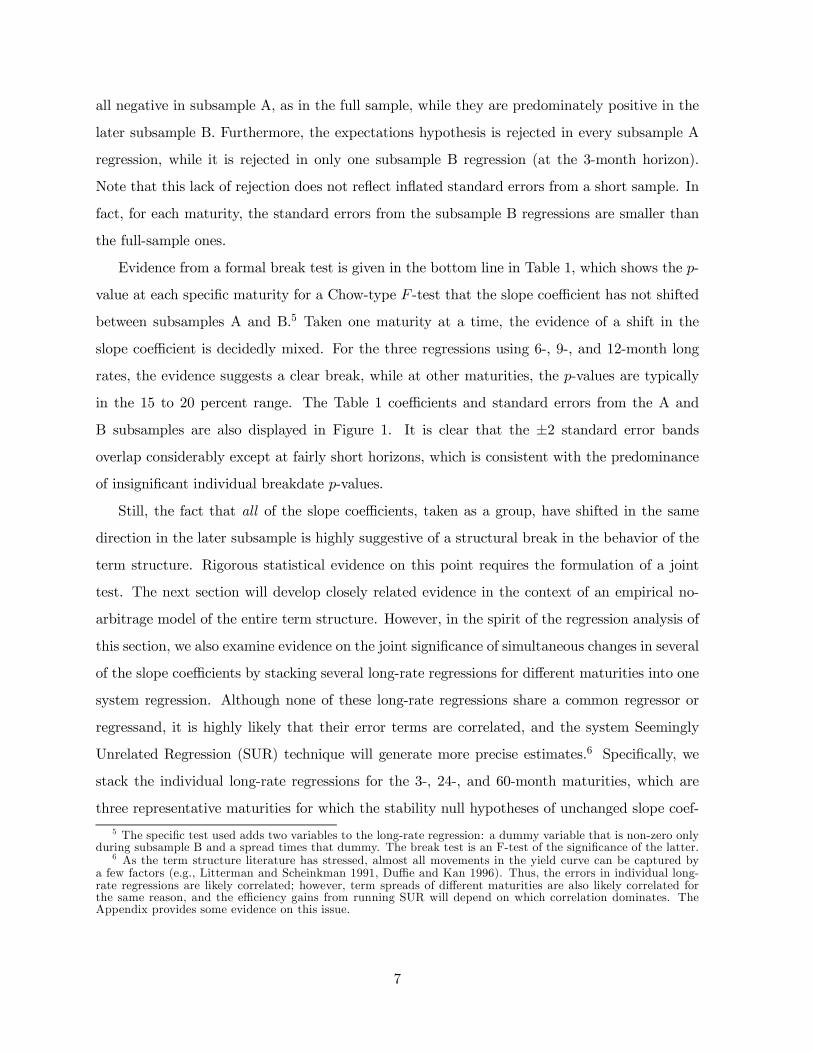
Evidence from a formal break test is given in the bottom line in Table 1, which shows the p-
value at each speci…c maturity for a Chow-type F -test that the slope coe¢cient has not shifted
between subsamples A and B.5 Taken one maturity at a time, the evidence of a shift in the
slope coe¢cient is decidedly mixed. For the three regressions using 6-, 9-, and 12-month long
rates, the evidence suggests a clear break, while at other maturities, the p-values are typically
in the 15 to 20 percent range. The Table 1 coe¢cients and standard errors from the A and
B subsamples are also displayed in Figure 1. It is clear that the §2 standard error bands
overlap considerably except at fairly short horizons, which is consistent with the predominance
of insigni…cant individual breakdate p-values.
Still, the fact that all of the slope coe¢cients, taken as a group, have shifted in the same
direction in the later subsample is highly suggestive of a structural break in the behavior of the
term structure. Rigorous statistical evidence on this point requires the formulation of a joint
test. The next section will develop closely related evidence in the context of an empirical no-
arbitrage model of the entire term structure. However, in the spirit of the regression analysis of
this section, we also examine evidence on the joint signi…cance of simultaneous changes in several
of the slope coe¢cients by stacking several long-rate regressions for di¤erent maturities into one
system regression. Although none of these long-rate regressions share a common regressor or
regressand, it is highly likely that their error terms are correlated, and the system Seemingly
Unrelated Regression (SUR) technique will generate more precise estimates.6 Speci…cally, we
stack the individual long-rate regressions for the 3-, 24-, and 60-month maturities, which are
three representative maturities for which the stability null hypotheses of unchanged slope coef-5 The speci…c test used adds two variables to the long-rate regression: a dummy variable that is non-zero only
during subsample B and a spread times that dummy. The break test is an F-test of the signi…cance of the latter.6 As the term structure literature has stressed, almost all movements in the yield curve can be captured by
a few factors (e.g., Litterman and Scheinkman 1991, Du¢e and Kan 1996). Thus, the errors in individual long-rate regressions are likely correlated; however, term spreads of di¤erent maturities are also likely correlated forthe same reason, and the e¢ciency gains from running SUR will depend on which correlation dominates. TheAppendix provides some evidence on this issue.
7

…cients were not rejected in the individual regressions. The system regression for these three
maturities is24
i2,t+1 ¡ i3,ti23,t+1 ¡ i24,ti59,t+1 ¡ i60,t
35 =
24
α3α24α60
35 +
24
β3 0 00 β24 00 0 β60
35
24
(i3,t ¡ it)/2(i24,t ¡ it)/23(i60,t ¡ it)/59
35 +
24
ε3,tε24,tε60,t
35 . (2.4)
The estimation results for this SUR regression are shown in Table 2 for the full sample and
for subsamples A and B. The slope coe¢cient estimates in subsamples A and B continue to
show the same stark quantitative di¤erences apparent in the individual regressions in Table 1;
however, the coe¢cient standard errors are, on average, about half as large in magnitude. This
greater precision sharpens inference, and for these three maturities (which again were chosen for
their individual non-rejection of stability null), the p-value of .006 clearly rejects the joint null
hypothesis of no change in the three slope coe¢cients between the A and B subsamples. These
system break test results are representative of other combinations of three or more yields.7
Finally, while we have considered a speci…c breakdate, based on a prior view of the timing of
changes in the behavior of aggregate output, in‡ation, and monetary policy, it is also useful to
consider more generally the testing of the null of parameter stability without such a prior. To do
this, we consider all possible breakdates in the middle 80 percent of the full sample, and calculate
a Chow-type test statistic at each of these breakdates. Figure 2 shows this set of test statistics
as well as two 5 percent critical values. The less stringent one—the lower dashed line—is the
usual χ2 boundary for the hypothesis that a speci…c (a priori) known breakdate is signi…cant.
The more stringent one—the upper dashed line—is based on a test that does not assume any
prior knowledge about potential breakdates. It tests the signi…cance of the maximum value of
all Chow-type test statistics calculated at all possible breakdates in the middle 80 percent of the
sample, and was derived by Andrews (1993).8 Applied to all possible breakdates for the system
regression (2.2), the break test statistic is well above the 5 percent critical value of Andrews for
several years, especially during the late 1980s. This evidence supports our earlier selection of a
breakdate, though, not surprisingly, the test is not sensitive enough to single out just one date.
In summary, we take the regression results as indicative of a break in term structure behavior
around the middle of the 1980s. Determining the nature of that break in terms of changes in7 The expectations hypothesis, namely, that all three slope coe¢cients equal unity, is also rejected in the
system regressions in Table 2. For subsample B, this rejection re‡ects the low value of β3.8 For our application, in which the variables are not highly persistence, it appears from various small-sample
simulation studies that this asymptotic distribution is appropriate (see Diebold and Chen 1996 and O’Reilly andWhelan 2004).
8

the dynamics of the short rate, of risk, or of the pricing of that risk is the subject of the rest of
our analysis.
3. Estimating Subsample No-Arbitrage Models
In the preceding section, we provided regression evidence of a signi…cant shift in the behavior of
the term structure during the 1980s. In this section, we estimate dynamic term structure models
that can capture that shift in behavior. The framework we use is a standard no-arbitrage
representation from the empirical bond pricing literature that assumes no opportunities for
…nancial arbitrage across bonds of di¤erent maturities.
We focus on a two-factor, Gaussian, a¢ne, no-arbitrage term structure model, or an A0(2)
model as de…ned in Dai and Singleton (2000). The model features a constant volatility of
term structure factors but the risk pricing is state-dependent, which implies conditionally het-
eroskedastic risk premiums. Dai and Singleton (2002) compare the performance of di¤erent
dynamic term structure models and …nd that this type of speci…cation performs the best in
matching the full-sample long-rate regression coe¢cients.9
The model is formulated in discrete time.10 The state vector relevant for pricing bonds is
assumed to be summarized by two latent term structure factors, Lt and St. These are stacked
in the vector Ft = (Lt, St)0, which follows a Gaussian VAR(1) process:
Ft = ρFt¡1 + §εt, (3.1)
where εt is i.i.d. N(0, I2), § is diagonal, and ρ is a 2 £ 2 lower triangular matrix. The short
(one-month) rate is de…ned to be a linear function of the latent factors:
it = δ0 + Lt + St = δ0 + δ01Ft. (3.2)
Without loss of generality, this implicit de…nition of δ1 implies unitary loadings of the two factors
on the short rate because of the normalization of the unobservable factors. Finally, following
Constantinides (1992), Dai and Singleton (2000, 2002), Du¤ee (2002), and others, the prices of
risk associated with the conditional volatility in the Lt factor, denoted ¤L,t, and in the St factor,9 Dai and Singleton (2000) use a three-factor model, but following Rudebusch and Wu (2004) we obtain an
adequate …t, especially in subsample B, with two factors.10 This model is a standard …nance representation; see Dai and Singleton (2000) and Rudebusch and Wu (2004)
for references and discussion.
9
denoted ¤S,t, are de…ned to be linear functions of the factors:
¤t =·
¤L¤S
¸
t= λ0 + λ1Ft. (3.3)
Note that if all of the elements of λ1 are zero, then the price of risk and the risk premium are
constant, and, in this special case, the expectations hypothesis holds.
Under the no-arbitrage assumption, the logarithm of the price of a j-period nominal bond
is a linear function of the factors
ln(bj,t) = Aj + B0jFt, (3.4)
where the coe¢cients Aj and Bj are recursively de…ned by
A1 = ¡δ0; B1 = ¡δ1
Aj+1 ¡ Aj = B0j(¡§λ0) +
12B0
j§§0Bj + A1
Bj+1 = B0j(ρ ¡ §λ1) + B1; j = 1, 2, ..., J. (3.5)
Given this bond-pricing formula, the continuously compounded yield to maturity ij,t of a j-
period nominal zero-coupon bond is given by the linear function
ij,t = ¡ ln(bj,t)/j = Aj + B0jFt, (3.6)
where Aj = ¡Aj/j and Bj = ¡Bj/j.
The above model is estimated by maximum likelihood using end-of-month data on U.S.
Treasury zero-coupon bond yields of maturities 1, 3, 12, 36, and 60 months (the yields are
expressed at an annual rate in percent.) In estimating the model, the mean of the short rate δ0
is set to the unconditional mean of the short rate in each subsample period (and λ0L is normalized
to zero). Therefore, the estimated model parameters for factor dynamics, risk pricing, and factor
shocks are
ρ =·
ρL 0ρSL ρS
¸, λ0 =
·0λ0
S
¸, λ1 =
·λ1
LL λ1LS
λ1SL λ1
SS
¸, and § =
·σL 00 σS
¸.
In addition, following standard practice in the literature, the 1-month and 60-month bond yields
are assumed to be measured without error, while bond yields of the other three maturities are
measured with i.i.d. shocks with mean zero. The standard errors of these measurement errors
are denoted σ3, σ12, σ36. Finally, out of concern that the model may be over-parameterized,
10
we impose certain zero restrictions on λ0 and λ1 on the entries with insigni…cant estimates in
a preliminary round of model estimation. This procedure is common in the …nance literature
(e.g., Dai and Singleton 2000 and Ang and Piazzesi 2003) and introduces little change to the
value of the likelihood function.
We estimate the model separately on the full sample of data (1970-2002) and on subsamples A
(1970-1987) and B (1988-2002) as suggested by the results in Section 2. The maximum likelihood
estimates of the model in di¤erent sample periods, along with their estimated standard errors
and the value of the log-likelihood function, are displayed in Table 3. The most important result
in Table 3 is that the hypothesis of a single unchanged data-generating process during the full
sample is rejected at any signi…cance level—the likelihood ratio test statistic, which follows a
χ2(12) under the hypothesis, is 481.88. This evidence provides another strong rejection of the
joint stability hypothesis, consistent with the SUR test results of Table 2, and it helps validate
the splitting of the sample.
The two subsample models exhibit interesting similarities and di¤erences in parameter es-
timates. As is typically found, both the subsample A and subsample B models have a very
persistent Lt factor (ρL ¼ .99) and a less persistent St factor (ρS ¼ .95). These two factors
are often given the labels “level” and “slope,” respectively, since a positive shock to Lt pushes
up yields at all maturities while a positive shock to St predominantly pushes up yields at short
maturities. Indeed, the factor loadings of both of our subsample estimated models are consistent
with such a designation. Although both level and slope are a bit more persistent during the
later subsample, a more striking di¤erence is found in the factor shock volatilities in the two
subsample periods. In particular, the volatilities of both factor shocks are signi…cantly larger in
the earlier subsample than in the later subsample. The estimates of the standard deviations of
the level and slope factor shocks are 41 and 60 basis points during subsample A, but only 15 and
42 basis points in subsample B.11 This …nding is consistent with the view that 1970 to 1987 is a
turbulent period for …nancial markets and the macroeconomy, while the more recent period has
lower …nancial risks and a more tranquil economy. Finally, there is also a clear di¤erence in risk
pricing in the two subsamples. The subsample A estimates of the elements of λ1 are uniformly
larger than in subsample B. Time variation in risk premiums in this model solely re‡ects the
time variation in the price of risk (as the volatilities of risks are constant), which is a linear11 Interestingly, past regime-switching studies (Gray 1996, Ang and Bekaert 2002, and Dai, Singleton and Yang
2003) also …nd that the term structure factors exhibit less mean reversion (i.e., more persistence) in regimes withlow volatilities of term structure risks.
11
function of the factors. Therefore a larger λ1 implies a larger variation in the risk price for a
given time variation of factors. In other words, for same level of factor volatilities, the larger
estimates of λ1 in the earlier subsample will generate larger risk premiums.
Overall, the subsample model estimates appear consistent with the notion of a shift in term
structure behavior as suggested by the regression evidence. In the next section, we will link the
di¤erences in model parameter estimates to the di¤erent regression results.
4. Accounting for the Shift in Term Structure Behavior
Section 2 provided evidence of a signi…cant break in the estimated coe¢cients in various long-
rate term structure regressions, and Section 3 provided evidence of a signi…cant break in a
no-arbitrage dynamic term structure model. In this section, we link these two results together
by investigating the ability of the two subsample no-arbitrage models (estimated in Section 3)
to account for the long-rate regression results through changing factor and risk price dynamics .
Our examination focuses on long-rate regression coe¢cients implied by a particular no-
arbitrage term structure representation. For a given no-arbitrage model of the form described
in Section 3, the population value of the long-rate regression coe¢cient for maturity m is given
by
βm ´ cov[(im¡1,t+1 ¡ im,t), (im,t ¡ i1,t)/(m ¡ 1)]var[(im,t ¡ i1,t)/(m ¡ 1)]
=cov[(B0
m¡1Ft+1 ¡ B0mFt), (B0
mFt ¡ B01Ft)]
var[B0mFt ¡ B0
1Ft](m ¡ 1)
=(B0
m¡1ρ ¡ B0m)(B0
mρ ¡ B01)0
(B0mρ ¡ B0
1)(B0mρ ¡ B0
1)0(m ¡ 1) (4.1)
where the Bm’s are the factor loadings de…ned in Section 3 and denotes the unconditional
variance-covariance matrix of the two factors in Ft. From equation (3.5), note that the Bm’s
are determined by §, λ1, and ρ—that is, by the covariance of the factor shocks, the sensitivity
of the price of risk to the factors, and the parameters of the autoregressive dynamics of the
factors, respectively. From equation (3.1), note that depends on the parameters § and ρ.
Therefore, the population regression coe¢cients associated with di¤erent no-arbitrage model
structural estimates are straightforward to compute.
The implied long-rate regression coe¢cients associated with the subsample model estimates
shown in Table 3 are given in Figures 3 and 4, for subsamples A and B, respectively. The dark
12
solid lines in these …gures plot the population βm coe¢cients at all bond maturities that are
implied by the subsample A and B model parameter estimates. These implied model population
estimates match the historical regression results fairly well. For subsample A (Figure 3), the
model-implied regression coe¢cients decrease quite rapidly as the maturity of the long rate
increases. Although the population coe¢cients are not quite as low as the historical estimates
for maturities less than 48 months, there is a fairly close match at longer maturities. For
subsample B (Figure 4), the model-implied projection coe¢cients are all positive and quite close
to the empirical regression estimates.
In order to account for possible small-sample biases, we also simulate data from each model
and calculate the regression coe¢cients in repeated …nite samples. Speci…cally, we take random
draws of εt (with the number determined by the particular sample period under investigation),
simulate data from the no-arbitrage model, and compute the long-rate projection coe¢cients.
This procedure is repeated 1000 times, and Figures 3 and 4 also plot the medians and 90 percent
frequency or con…dence bands from these simulations. In both …gures, the median estimates
from the simulations lie very close to the population estimates, indicating that the small-sample
biases are fairly modest in this application (which is consistent with the results reported in the
Appendix). In addition, the empirical estimates typically lie inside the 90 percent con…dence
bands of the model simulations.
The source for the di¤erences in the term structure dynamics between the two subsamples
can be illuminated with model perturbations. Speci…cally, we look at the e¤ect on a long-rate
regression coe¢cient from changing a subset of the model parameters from their subsample
A estimated values to their subsample B estimated values. This model variation can uncover
the speci…c factors driving the di¤erent subsample regression results. However, because the
long-rate regression coe¢cients are nonlinear functions of the model parameters, the e¤ect of
changing a particular model parameter depends on the exact constellation of all of the other
parameters. To reduce the number of model permutations to a more manageable size, we focus
on three blocks of parameters—in §, λ1, and ρ—as sets that contain either all subsample A
estimates or all subsample B estimates. For example, the ρLL, ρSS , and ρSL in ρ are all either
from subsample A or subsample B. Thus, there are only eight possible combinations of the two
subsample estimates of §, λ1, and ρ to consider. Each of each these eight cases is identi…ed by
a parameter triple, with ρA, §A, λA, ρB, §B, and λB representing the estimates of ρ, §, and λ1
13
in subsamples A and B, respectively.
The model perturbation results obtained from varying these three sets of parameters are
given in Table 4. For conciseness, the table only displays the e¤ect on the β120 coe¢cient,
but our conclusions generalize to the other long-rate maturities as well. The top line shows
the change in the population estimate of β120 resulting from a shift from all subsample A no-
arbitrage parameter estimates (denoted as the ρA, §A, λA model) to all subsample B parameter
estimates (denoted as ρB, §B, λB). This change, which is 2.88, is also the di¤erence between
the right-hand-side endpoints of the solid lines in Figures 3 and 4. The rest of Table 4 provides
a quantitative accounting of the source of this change. Speci…cally, the next block of lines
investigates a change in just the autoregressive parameters from ρA to ρB, holding …xed the
other parameters across the four possible permutations of § and λ1 (namely, §A, λA; §A, λB;
§B, λA; §B, λB). The average e¤ect of such a change in factor dynamics would cause β120 to
decrease by 1.04—that is, β120 is pushed in the opposite direction from what was observed. In
contrast, as shown in the middle lines, the shift in the factor shock volatility parameters from
§A to §B induces, on average, a 0.46 increase in β120, which is a modest step in the observed
direction of change. Finally, as shown in the bottom panel of Table 4, the change in the risk
pricing parameters from λA to λB more than accounts for the total observed change in β120.
Therefore, the risk pricing parameters appear crucial in generating the changing pro…le of
the long-rate regression coe¢cients across the two subsamples. The more factor-sensitive risk
pricing in subsample A—since the subsample A estimates of λ1 are larger than in subsample
B—generates greater time variation in the risk premiums for a given level of factor volatilities.
These more variable subsample A term premiums induce greater deviations from the expecta-
tions hypothesis and push the βm estimates below those in subsample B. This e¤ect is reinforced
to a limited extent by the higher variances of the factor shocks in the …rst subsample (since the
elements of §A are larger than those of §B). These higher factor shock variances induce higher
factor volatilities and hence greater time variation in the price of risk and risk premiums. How-
ever, a partial o¤set to the above two factors comes from the higher autoregressive parameters
in the later subsample. Speci…cally, because the elements of ρB are higher than those of ρA,
these work to boost the volatility of the factors and risk premiums in subsample B and lower
the regression coe¢cients.12
12 In addition, we have found that a higher persistence of the factors, even holding the volatility of the fac-tors constant (as opposed to the holding constant the volatility of the factor shocks), leads to lower regression
14

Table 5 reports on a model permutation procedure that considers individual parameters
instead of just blocks of parameters. There are eight key individual model parameters in ρ, §,
and λ1: ρLL, ρSS, ρSL, σL, σS, λ1LL, λ1
LS, and λ1SS . Table 5 provides the average e¤ect on β120
of changing each one of these coe¢cients from its subsample A estimate to its subsample B
estimate, holding the other coe¢cients …xed.13 These results further narrow the source of the
upward shift in the long-rate regression coe¢cients in the later subsample to just a few model
parameters, all of which are related to the level factor. In particular, the two most in‡uential
parameters are λ1LL and λ1
LS, which control the way in which the price of risk that is attached
to ‡uctuations in the level factor varies with the magnitude of level and slope. The reduced size
of these risk pricing parameters in subsample B can account on their own for the shift in the
long-rate regression coe¢cients across the two subsamples. The reduction in σL, the variance of
shocks to level, also plays some role by reducing level factor volatility (and the associated risk
premium variability), but this e¤ect is o¤set by the increase in the level factor autoregressive
parameter ρLL, which tends to boost the level factor variability.
To summarize, the standard no-arbitrage bond pricing model suggests that the recent histor-
ical shift in term structure behavior predominantly re‡ects a change in the way investors price
risk associated with the level factor. Changes in factor dynamics and factor shock volatility
appear to have played a relatively modest role. These term structure results may also help
illuminate the nature of the moderation and transformation of the U.S. economy that occurred
in the 1980s. As noted in the introduction, one hypothesis is that there was a run of less volatile
economic shocks in the more recent period. Our estimates support the presence of less volatile
factor shocks in the recent subsample; however, the e¤ect of this change on the behavior of
the term structure appears modest. Instead, our estimates indicate that there was a important
change in the dynamics of the economy that e¤ected risk pricing. The next section elaborates
on this interpretation using a no-arbitrage macro-…nance model that links movements in the
level factor to observable variables in the economy.
coe¢cients.13 For investigating the e¤ects of a change in any given parameter, there are 128 possible mixed sample A and
B permutations for the other seven parameters. (Note that λ1SL is zero in both samples.) We do not investigate
all of these permutations; instead, Table 5 provides the average change in β120 using a representative sample ofeight of these con…gurations using the same blocks of parameters in Table 4.
15

5. A Macro-Finance Perspective on the Term Structure Shift
The analysis so far suggests that an important transformation occurred in the U.S. economy
in the 1980s regarding the behavior of the level factor and, in particular, the pricing of risk
associated with that factor. A natural next step is to provide an economic interpretation of
these changes. We pursue this task in the structural macro-…nance model of Rudebusch and Wu
(2004), which we describe brie‡y before considering some model perturbations.
The Rudebusch-Wu macro-…nance model combines the above canonical no-arbitrage term
structure representation with elements from a standard macroeconomic model. A key point
of intersection between the …nance and macroeconomic speci…cations is the short-term interest
rate. The short rate remains a linear function of two latent term structure factors as in the
…nance model, so
it = δ0 + Lt + St. (5.1)
As demonstrated in Rudebusch and Wu (2004), however, there is a close connection among these
level and slope factors and a simple Taylor (1993) rule for monetary policy:
it = r¤ + π¤t + gπ(πt ¡ π¤t ) + gyyt, (5.2)
where r¤ is the equilibrium real rate, π¤t is the central bank’s in‡ation target, πt is the annual
in‡ation rate, and yt is a measure of the output gap. This link re‡ects the fact that the Federal
Reserve sets the short rate in response to macroeconomic data in an attempt to achieve its
goals of output and in‡ation stabilization. Therefore, level and slope are not simply modeled
as purely autoregressive time series; instead, they form elements of a monetary policy reaction
function. In particular, Lt is interpreted the medium-term in‡ation target of the central bank
as perceived by private investors. Investors are assumed to modify their views of the underlying
rate of in‡ation slowly, as actual in‡ation, πt, changes, so Lt is linearly updated by news about
in‡ation:14
Lt = ρLLt¡1 + (1 ¡ ρL)πt + εL,t. (5.3)
The slope factor St captures the Fed’s dual mandate to stabilize the real economy and keep
in‡ation close to its medium-term target level. Speci…cally, St is modeled as the Fed’s cyclical
response to deviations of in‡ation from its target, πt ¡ Lt, and to deviations of output from its14 As shown in Rudebusch and Wu (2004), Lt is primarily associated with yields of maturities from 2 to 5 years,
which is an important indication of the relevant horizon for the associated in‡ation expectations.
16

potential, yt:
St = ρSSt¡1 + (1 ¡ ρS)[gyyt + gπ(πt ¡ Lt)] + uS,t (5.4)
uS,t = ρuuS,t¡1 + εS,t. (5.5)
In addition, a very general speci…cation of the dynamics of St is adopted that allows for both
policy inertia and serially correlated elements not included in the basic Taylor rule.15
The dynamics of the macroeconomic determinants of the short rate are then speci…ed with
fairly standard New Keyesian equations for in‡ation and output (adjusted for monthly data):
πt = µπLt + (1 ¡ µπ)[απ1πt¡1 + απ2πt¡2] + αyyt¡1 + επ,t (5.6)
yt = µyEtyt+1 + (1 ¡ µy)[βy1yt¡1 + βy2yt¡2] ¡ βr(it¡1 ¡ Lt¡1) + εy,t . (5.7)
That is, in‡ation responds to the public’s expectation of the medium-term in‡ation goal (Lt),
two lags of in‡ation, and the output gap. Output depends on expected output, lags of output,
and a real interest rate.
The speci…cation of long-term yields in the macro-…nance model follows the standard no-
arbitrage formulation described in Section 3. Accordingly, the state space of the combined
macro-…nance model can be expressed by equation (3.1) with the state vector Ft rede…ned to
include output and in‡ation. The dynamic structure of this transition equation is determined by
equations (5.3) through (5.5). There are four structural shocks, επ,t, εy,t, εL,t, and εS,t, which are
assumed to be independently and normally distributed. The short rate is determined by (5.1).
For pricing longer-term bonds, the risk price associated with the structural shocks is assumed
to be a linear function of only Lt and St, which matches the formulation in Section 3 and allows
for easy comparison.16 However, it should be noted that the macroeconomic shocks επ,t and εy,t
are able to a¤ect the price of risk through their in‡uence on πt and yt and, therefore, on the
latent factors, Lt and St.
The estimates of this macro-…nance model from Rudebusch and Wu (2004), which are based
on U.S. term structure data that are essentially from subsample B (1988 to 2000), are shown in
Table 6. As above, the factor Lt is very persistent, with a ρL estimate of 0.989, which implies a15 If ρu = 0, the dynamics of St arise from monetary policy partial adjustment; conversely, if ρS = 0, the
dynamics re‡ect the Fed’s reaction to serially correlated information or events not captured by output andin‡ation. Rudebusch (2002) shows that the latter is often confused with the former in empirical applications.
16 Therefore, λ1 continues to have just four potentially non-zero entries (λ1LL, λ1
LS , λ1SL, and λ1
SS), thus greatlyreducing the number of parameters to be estimated.
17

small but signi…cant response to actual in‡ation. The monetary policy interpretation of the slope
factor is supported by the reasonable estimated in‡ation and output response coe¢cients, gπ
and gy, which are 1.25 and 0.20, respectively. These values, as well as the estimated parameters
describing the in‡ation and output dynamics, appear to be in line with other estimates in the
literature.
We next turn to the implied long-rate regression coe¢cients from this model.17 As before,
we conduct a model simulation exercise in which repeated samples of data are generated from
the macro-…nance model and used in the calculation of regression coe¢cients. Figure 5 shows
median values of the regression coe¢cients obtained from the macro-…nance model simulated
data as a solid line. The coe¢cients are predominantly positive and decline from about 1 at
a very short maturity to slightly negative at a 120-month maturity. These estimates are a bit
closer to the actual historical estimates from the subsample B data (shown as the dotted line)
than the coe¢cients implied by the estimated subsample B no-arbitrage model from Sections 3
and 4 (the dashed line).
The analysis in Sections 3 and 4 suggested that changes in the conditional volatility of the
level factor and in the pricing of level factor risk were the most important factors in accounting
for the shift in long-rate regression coe¢cients. This same issue can be examined in the macro-
…nance model. In particular, as noted above, the key parameters λ1LL, λ1
LS , and σL play the
same role in both models. The e¤ect of changing these parameters in the macro-…nance model is
shown in Table 7, which, as in Tables 4 and 5, focuses on just the coe¢cient β120 for conciseness.
The …rst three lines of Table 7 show the e¤ect on β120 of changing λ1LL, λ1
LS , and σL from their
estimates in Table 6 (-0.0045, 0.0168, and 0.342, respectively) to their subsample A estimates
in Table 3 (-0.0146, 0.0342, and 0.41, respectively).18 Increasing (in absolute value) λ1LS and σL
gives clearly lower estimates of β120, while changing λ1LL has little e¤ect on its own. However,
the combination of all three changes—line 4—shifts β120 down by a substantial 2.05. That is, as
above in the basic no-arbitrage model, the risk pricing and dynamics of the level factor appear
crucial for accounting for the shift in term structure behavior.
More importantly, the macro-…nance model provides an economic interpretation of this shift.17 Hördahl, Tristani, and Vestin (2004) also examine long-rate regression coe¢cients from a macro-…nance
model for German data.18 Another experiment that we are investigating in further work would be to estimate the macro-…nance model
for sample A and conduct a comparison as in Section 4. This may be problematic because the estimated policyrule of sample A often induces nonstationarity in forward-looking rational expectations macroeconomic models(see Rudebusch 2004).
18
Since the level factor re‡ects the perceived in‡ation target, the macro-…nance explanation of the
shift in term structure behavior is that during the 1970s and early 1980s investors had a very
di¤erent view of the medium-term outlook for in‡ation than they did later on. Early investors
appear to have viewed the in‡ation goal as particularly uncertain, in the sense that it had
a greater conditional volatility (higher σL) and that its price of risk was more sensitive to
‡uctuations in the economy (in particular, a higher λ1LS). This explanation is broadly consistent
with the view that expectations of the underlying goals for in‡ation were less …rmly anchored in
investors’ minds during the earlier subsample, which is a common interpretation of the historical
evolution of U.S. monetary policy. Alternatively, it could also be that changes to …nancial
markets or institutions allow investors to hedge interest rate risk better in the later subsample,
so that the risk compensation is less sensitive to changes in the economy.
Other changes in the economy may also have played a role in the shifting term structure
behavior. Many authors have noted that the volatilities of shocks to output and in‡ation are
signi…cantly larger in the 1970s than in the 1990s. To consider the possibility that the higher
conditional macroeconomic volatility in the earlier period helped account for the lower regression
coe¢cients, we increase the standard deviations of the output and in‡ation shocks, σπ and σy,
by 50 percent, which is the order of magnitude suggested by previous empirical work, including
Stock and Watson (2003) and Moreno (2004). As shown in the second line from the bottom in
Table 7, this model perturbation has little e¤ect on the estimate of β120. Another important
economic change that many estimated models of Federal Reserve behavior have highlighted
is the substantially lower responsiveness of monetary policy to in‡ation that occurred before
the 1980s.19 To consider the possibility that a lower in‡ation response parameter in the earlier
subsample may lower the regression coe¢cients, we lower the in‡ation response coe¢cient in the
monetary policy rule, gπ, by one-half, which is broadly in line with various empirical estimates.
The result, as shown in the bottom row of Table 7, is a very modest e¤ect on the estimate of
β120.19 See, for example, Fuhrer (1996), Judd and Rudebusch (1998), Clarida, Galí, and Gertler (2000), and Rude-
busch (2004) for discussion. In contrast to the in‡ation response coe¢cient, the evidence on a signi…cant changein the monetary policy output response coe¢cient is mixed.
19

6. Conclusion
As noted in the introduction, the existence of a shift in the behavior of the term structure would
not be surprising, given the dramatic changes in the economy over the past few decades. We
indeed document such a shift in the behavior of the term structure using a simple regression
technique as well as structural models. Our key result is that the volatility of term premiums
appears to have declined over time; furthermore, this decline appears to have been induced by
changes in the conditional volatility and price of risk of the term structure level factor, which
we suggest may be related to investors’ perceptions of the Fed’s in‡ation goals.
Of course, as many have noted, a shift in the conduct of monetary policy will likely lead
to a change in the behavior of the term structure (for example, Rudebusch 1995, Fuhrer 1996,
Kozicki and Tinsley 2001, and Cogley 2003). However, our results suggest that the linkage is
perhaps more subtle than is commonly appreciated. For example, although the Fed’s short rate
response to changes in in‡ation during the 1970s has been found to be less vigorous than in the
1990s, such a change—on its own—appears to have small direct e¤ects on the evolution of term
premiums and appears unlikely to account for the shift apparent in our empirical results. This
conclusion appears to mirror that of Stock and Watson (2003), who found small direct e¤ects of
monetary policy rule changes on macroeconomic volatility. However, our results do suggest that
broader, but likely closely related, shifts in the monetary policy environment may have played
an important role. In particular, a change in the perceptions of the in‡ation goals of the Fed
could alter the dynamic evolution of term premiums as well as short rates. Such a change may
re‡ect a greater willingness to anchor the in‡ation rate or a greater transparency about such
desires.
20
A. Appendix on Small-Sample Inference
In Section 2, we conduct inference on the expectations hypothesis and the hypothesis of stable
parameters using asymptotic distributions that have been called into question in certain circum-
stances (e.g., in Bekaert, Hodrick, and Marshall 1997b). In this section, we report monte carlo
simulations using the estimated models of Section 3 in order to explore the appropriateness of
this inference in small samples for our models.
Table A1 displays the results of testing the expectations hypothesis based on 1000 simulated
samples of size 396, 216, and 180 observations, respectively, for the full sample, subsample A,
and subsample B. Using these simulated data, the change in the 3-month rate and the change in
the 60-month rate are regressed on the on the 3- and 1-month spread and the 60- and 1-month
spread, respectively. Each entry in the table reports the frequency with which an F-test statistic
rejects the null expectations hypothesis, which is the hypothesis that the slope coe¢cient (or a
pair of slope coe¢cients) is equal to one. These rejections are calculated using the standard 5
percent asymptotic critical values. In the top panel of Table A1, model simulations are based
on parameter estimates from each sample of data (given in Table 3) except that the price of
risk is set to be a constant (λ1 is set equal to 0). Constant risk prices in this term structure
model imply that risk premiums are constant; thus, the null expectations hypothesis is true and
the population slope regression coe¢cient is indeed one. In this case, the reported rejection
frequency is the empirical size of the F-test.
The …rst row of the top panel reports the frequency of rejection using as a data-generating
process the full-sample model estimates in Table 3 (again with λ1 set equal to 0). For the
individual long-rate regressions, the hypothesis that β3 = 1 is rejected 7.7 percent of the time,
and the hypothesis that β60 = 1 is rejected 6.7 percent of the time. These empirical sizes are
quite close to the 5 percent nominal size. The third entry of 5.7 percent gives the frequency of
simulated samples in which β3 = 1 and β60 = 1 were both rejected in the individual long-rate
regressions. This statistic provides a relevant comparison for the system SUR estimation, which
tests the joint null expectations hypothesis that β3 = β60 = 1. This joint test has an empirical
size of 7.7 percent. The second and third rows of Table A1 show that the F-test is only slightly
less well-sized when the data are simulated from the subsample A model estimates and the
subsample B model estimates (which may re‡ect the smaller samples in these cases).
The lower panel of Table A1 displays the frequency of rejections when the data are simulated
21
from the exact estimated models given in Table 3. In each of these models, λ1 6= 0, so the
price of risk is time-varying and the expectations hypothesis does not hold; thus, the rejection
frequencies in this panel indicate the empirical power of the F-test. The power of this test, given
our data-generating mechanism and sample sizes, is low (particularly for the 3-month maturity)
to moderate (for the 60-month maturity). The simulation results indicate some advantage to
running system SUR when testing the joint expectations hypothesis. When the simulations are
based on full-sample model estimates, the system regression correctly rejects the null in 24.2
percent of the draws, while the individual long-rate regressions reject the null on both 3- and
60-month maturities in only 6.2 percent of the draws. This pattern is similar when simulations
are based on subsample A estimates. When simulation is performed based on subsample B
estimates, however, the power in running individual long-rate regressions becomes quite small
— even smaller than the corresponding empirical size in the upper panel. This puzzle re‡ects two
o¤setting e¤ects on the regression coe¢cients: a downward pressure from the time-varying risk
prices and term premiums, and an upward small-sample bias as discussed in Bekaert, Hodrick,
and Marshall (1997b) which tends to push the coe¢cients back to unity. The e¤ect of small-
sample bias is overwhelmed in the full-sample and subsample A simulations when the risk price
variability is large, but it is quite important in the subsample B simulations when the risk price
movements are small. However, the SUR reports smaller standard errors, so the power in running
the SUR is much higher than for individual long-rate regressions. This again underscores the
e¢ciency gains from the SUR.
Table A2 displays the frequency of rejection of a Chow-type test of the null hypothesis,
namely, that there is no di¤erence in the slope coe¢cient (or coe¢cients) between the earlier and
later subsamples. Each entry is based on 1000 simulations of 396 observations and reports the
frequency of the test statistic exceeding the 5 percent theoretical critical value, which indicates
rejection of the null hypothesis of no breakpoint. First consider the empirical size of the test.
In the top panel, the full-sample model estimates are used exclusively, so the data are generated
under a single regime. The frequency of rejection is 5.1 percent for the 3-month regression, 3.8
percent for 60-month regression, and 2.7 percent for the system SUR, suggesting that the test
is fairly well-sized though with some tendency to reject the null hypothesis less frequently than
theory would predict.
The bottom panel of Table A2 provides results when the data-generating process contains a
22
regime switch. In particular, the …rst 216 observations of each simulation are drawn from the
model estimates in subsample A, and the remaining 180 observations are drawn from the model
estimates in subsample B. Thus the proportions of rejections in this panel indicate the empirical
power of the Chow test, which appears fairly high. The test correctly rejects the null 66 percent
of the time for the 3-month rate regression and 64.8 percent of the time for the 60-month rate
regression. For the joint hypothesis, the structural stability null is rejected 54.8 percent of
the time with both individual regressions, which is lower than the 60.9 percent rejection rate
obtained with SUR, suggesting some modest e¢ciency gains to system estimation.
23
References
[1] Andrews, Donald (1993), “Tests for Parameter Instability and Structural Change withUnknown Change Point,” Econometrica 61, 821-856.
[2] Ang, Andrew and Geert Bekaert (2002), “Regime Switches in Interest Rates,” Journal ofBusiness and Economic Statistics 20(2), 163-182.
[3] Ang, A. and M. Piazzesi (2003), “No-Arbitrage Vector Autoregression of Term StructureDynamics with Macroeconomic and Latent Variables,” Journal of Monetary Economics 50,745-787.
[4] Backus, D., S. Foresi, A. Mozumdar, and L. Wu (2001), “Predictable Changes in Yieldsand Forward Rates,” Journal of Financial Economics 59(3), 281-311.
[5] Bansal, R. and H. Zhou (2002), “Term Structure of Interest Rates with Regime Shifts,”Journal of Finance 57, 1997-2043.
[6] Bekaert, Geert, Robert J. Hodrick, and David A. Marshall (1997a), “Peso Problem Expla-nations for Term Structure Anomalies,” NBER working paper no. 6147.
[7] Bekaert, Geert, Robert J. Hodrick, and David A. Marshall (1997b), “On Biases in Tests ofthe Expectations Hypothesis of the Term Structure of Interest Rates,” Journal of FinancialEconomics 44, 309-348.
[8] Blanchard, Olivier, and John Simon (2001), “The Long and Large Decline in U.S. OutputVolatility,” Brookings Papers on Economic Activity 1, 135-164.
[9] Bliss, Robert R. (1997), “Testing Term Structure Estimation Methods,” Advances in Fu-tures and Options Research 9, 197-231, Greenwich, Conn. and London: JAI Press.
[10] Campbell, John Y., and Robert J. Shiller (1991), “Yield Spreads and Interest Rate Move-ments: A Bird’s Eye View,” Review of Economic Studies 58, 495-514.
[11] Clarida, Richard, Jordi Galí, and Mark Gertler (2000), “Monetary Policy Rules and Macro-economic Stability: Evidence and Some Theory,” Quarterly Journal of Economics 115,147-180.
[12] Cogley, Timothy (2003), “An Exploration of Evolving Term-Structure Relations,” manu-script, University of California-Davis.
[13] Constantinides, G.M. (1992), “A Theory of the Nominal Term Structure of Interest Rates,”Review of Financial Studies 5, 531-552.
[14] Dai, Q. and K.J. Singleton (2000), “Speci…cation Analysis of A¢ne Term Structure Mod-els,” Journal of Finance 55, 1943-1978.
[15] Dai, Q. and K.J. Singleton (2002), “Expectations puzzles, time-varying risk premia, anda¢ne models of the term structure,” Journal of Financial Economics 63, 415-441.
[16] Dai, Q., K.J. Singleton, and Wei Yang (2003), “Regime Shifts in a Dynamic Term StructureModel of U.S. Treasury Bond Yields,” Stanford University Working Paper.
24
[17] Dewachter, H. and M. Lyrio (2002), “Macro Factors and the Term Structure of InterestRates,” manuscript, Catholic University of Leuven.
[18] Diebold, Francis, and Celia Chen (1996), “Testing Structural Stability with EndogenousBreak Point: A Size Comparison of Analytic and Bootstrap Procedures,” Journal of Econo-metrics 70, 221-241.
[19] Diebold, Francis, Glenn D Rudebusch, and S. Boragan Aruoba (2004), “The Macroeconomyand the Yield Curve: A Dynamic Latent Factor Approach,” manuscript, Federal ReserveBank of San Francisco, forthcoming in the Journal of Econometrics.
[20] Du¤ee, Gregory R. (2002), “Term Premia and Interest Rate Forecasts in A¢ne Models,”Journal of Finance 57, 405-443.
[21] Du¤ee, Gregory R. (2004), “A No-Arbitrage Term Structure Model Without Latent Fac-tors,” manuscript, University of California – Berkeley.
[22] Du¢e, D. and R. Kan (1996), “A Yield-Factor Model of Interest Rates,” MathematicalFinance 6, 379-406.
[23] Fuhrer, Je¤rey C. (1996), “Monetary Policy Shifts and Long-Term Interest Rates,” TheQuarterly Journal of Economics 111, 1183-1209.
[24] Gray, Stephen F. (1996), “Modeling the Conditional Distribution of Interest Rates as aRegime-Switching Process,” Journal of Financial Economics 42, 27-62.
[25] Hamilton, J.D. (1988), “Rational-Expectations Econometric Analysis of Changes in Regime:An Investigation of the Term Structure of Interest Rates,” Journal of Economic Dynamicsand Control 12, 385-423.
[26] Hördahl, Peter, Oreste Tristani, and David Vestin (2004), “A Joint Econometric Modelof Macroeconomic and Term Structure Dynamics,” manuscript, European Central Bank,forthcoming in the Journal of Econometrics.
[27] Judd, John, and Glenn Rudebusch (1998), “Taylor’s Rule and the Fed: 1970-1997,” Eco-nomic Review, Federal Reserve Bank of San Francisco, no. 3, 3-16.
[28] Kim, Chang-Jin, and Charles R. Nelson (1999), “Has the U.S. Economy Become MoreStable? A Bayesian Approach Based on a Markov-Switching Model of the Business Cycle,”The Review of Economics and Statistics 81, 608-616.
[29] Kozicki, Sharon, and P.A. Tinsley (2001), “Shifting Endpoints in the Term Structure ofInterest Rates,” Journal of Monetary Economics 47, 613-652.
[30] Lange, Joe, Brian Sack, and William Whitesell (2003), “Anticipations of Monetary Policyin Financial Markets,” Journal of Money, Credit, and Banking 35(6), 889-909.
[31] Litterman, Robert, and Jose A. Scheinkman (1991), “Common Factors A¤ecting BondReturns,” Journal of Fixed Income 1, 54-61.
[32] Mankiw, N.Gregory, and Je¤ A. Miron (1986), “The Changing Behavior of the Term Struc-ture of Interest Rates,” The Quarterly Journal of Economics 101, 211-228.
25
[33] McConnell, Margaret M., and Gabriel Perez-Quiros (2000), “Output Fluctuations in theUnited States: What has Changed Since the Early 1980’s,” American Economic Review90(5), 1464-1476.
[34] Moreno, Antonio (2004), “Reaching In‡ation Stability,” Journal of Money, Credit, andBanking 36, 801-825.
[35] O’Reilly, Gerard, and Karl Whelan (2004), “Has Euro-Area In‡ation Persistence ChangedOver Time?” Working Paper.
[36] Piazzesi, Monika (2003), “Bond Yields and the Federal Reserve,” manuscript, Journal ofPolitical Economy, forthcoming.
[37] Rudebusch, Glenn D. (1995), “Federal Reserve Interest Rate Targeting, Rational Expecta-tions, and the Term Structure,” Journal of Monetary Economics 24, 245-274.
[38] Rudebusch, Glenn D. (2002), “Term Structure Evidence on Interest Rate Smoothing andMonetary Policy Inertia,” Journal of Monetary Economics 49, 1161-1187.
[39] Rudebusch, Glenn D. (2004), “Assessing the Lucas Critique in Monetary Policy Models,”manuscript, forthcoming in the Journal of Money, Credit, and Banking.
[40] Rudebusch, Glenn D., and Tao Wu (2004), “A Macro-Finance Model of the Term Structure,Monetary Policy, and the Economy,” Working Paper.
[41] Stock, James H., and Mark W. Watson (2003), “Has the Business Cycle Changed? Evidenceand Explanations,” in Monetary Policy and Uncertainty, Federal Reserve Bank of KansasCity, 9-56.
[42] Taylor, John B. (1993), “Discretion versus Policy Rules in Practice,” Carnegie-RochesterConference Series on Public Policy 39, 195-214.
[43] Watson, Mark W. (1999), “Explaining the Increased Variability in Long-Term InterestRates,” Federal Reserve Bank of Richmond Economic Quarterly 85(4), 71-96.
[44] Wu, Tao (2001), “Macro Factors and the A¢ne Term Structure of Interest Rates,” manu-script, Federal Reserve Bank of San Francisco.
26
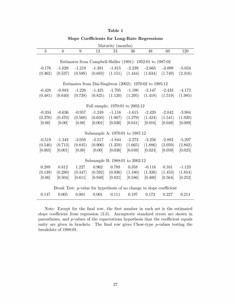
Table 1
Slope Coe¢cients for Long-Rate Regressions
Maturity (months)3 6 9 12 24 36 48 60 120
Estimates from Campbell-Shiller (1991): 1952:01 to 1987:02-0.176 -1.029 -1.219 -1.381 -1.815 -2.239 -2.665 -3.099 -5.024(0.362) (0.537) (0.598) (0.683) (1.151) (1.444) (1.634) (1.749) (2.316)
Estimates from Dai-Singleton (2002): 1970:02 to 1995:12-0.428 -0.883 -1.228 -1.425 -1.705 -1.190 -2.147 -2.433 -4.173(0.481) (0.640) (0.738) (0.825) (1.120) (1.295) (1.418) (1.519) (1.985)
Full sample: 1970:01 to 2002:12-0.334 -0.636 -0.957 -1.249 -1.116 -1.615 -2.420 -2.042 -3.984(0.370) (0.470) (0.560) (0.650) (1.007) (1.279) (1.424) (1.541) (1.920)[0.00] [0.00] [0.00] [0.001] [0.036] [0.041] [0.016] [0.048] [0.009]
Subsample A: 1970:01 to 1987:12-0.519 -1.342 -2.058 -2.517 -1.844 -2.273 -3.256 -2.882 -5.297(0.540) (0.713) (0.845) (0.906) (1.359) (1.665) (1.886) (2.059) (2.802)[0.005] [0.001] [0.00] [0.00] [0.036] [0.049] [0.024] [0.059] [0.025]
Subsample B: 1988:01 to 2002:120.289 0.812 1.227 0.962 0.788 0.358 -0.116 0.161 -1.123
(0.139) (0.280) (0.447) (0.592) (0.936) (1.180) (1.326) (1.453) (1.854)[0.00] [0.504] [0.611] [0.949] [0.821] [0.586] [0.400] [0.564] [0.252]
Break Test: p-value for hypothesis of no change in slope coe¢cient0.147 0.005 0.001 0.001 0.111 0.197 0.173 0.227 0.214
Note: Except for the …nal row, the …rst number in each set is the estimatedslope coe¢cient from regression (2.3). Asymptotic standard errors are shown inparentheses, and p-values of the expectations hypothesis that the coe¢cient equalsunity are given in brackets. The …nal row gives Chow-type p-values testing thebreakdate of 1988:01.
27
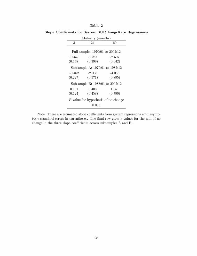
Table 2
Slope Coe¢cients for System SUR Long-Rate Regressions
Maturity (months)3 24 60
Full sample: 1970:01 to 2002:12-0.457 -1.267 -2.507(0.148) (0.399) (0.642)
Subsample A: 1970:01 to 1987:12-0.462 -2.008 -4.053(0.227) (0.571) (0.895)
Subsample B: 1988:01 to 2002:120.101 0.403 1.051
(0.124) (0.458) (0.790)
P -value for hypothesis of no change0.006
Note: These are estimated slope coe¢cients from system regressions with asymp-totic standard errors in parentheses. The …nal row gives p-values for the null of nochange in the three slope coe¢cients across subsamples A and B.
28
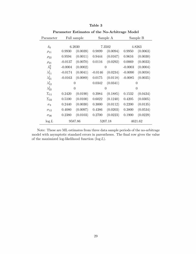
Table 3
Parameter Estimates of the No-Arbitrage Model
Parameter Full sample Sample A Sample B
δ0 6.2030 7.3502 4.8263ρ11 0.9930 (0.0039) 0.9899 (0.0094) 0.9950 (0.0063)ρ22 0.9594 (0.0011) 0.9444 (0.0167) 0.9616 (0.0030)ρ21 -0.0137 (0.0070) 0.0116 (0.0292) 0.0069 (0.0033)λ02 -0.0004 (0.0002) 0 -0.0003 (0.0004)
λ111 -0.0174 (0.0041) -0.0146 (0.0234) -0.0090 (0.0058)
λ121 -0.0163 (0.0089) 0.0175 (0.0118) -0.0085 (0.0035)
λ112 0 0.0342 (0.0341) 0
λ122 0 0 0
§11 0.2420 (0.0190) 0.3984 (0.1885) 0.1532 (0.0434)§22 0.5100 (0.0100) 0.6022 (0.1240) 0.4205 (0.0305)σ3 0.2440 (0.0030) 0.3000 (0.0112) 0.2200 (0.0135)σ12 0.4080 (0.0097) 0.4386 (0.0203) 0.3800 (0.0534)σ36 0.2380 (0.0103) 0.2700 (0.0223) 0.1900 (0.0229)
logL 9587.86 5207.18 4621.62
Note: These are ML estimates from three data sample periods of the no-arbitragemodel with asymptotic standard errors in parentheses. The …nal row gives the valueof the maximized log-likelihood function (log L).
29
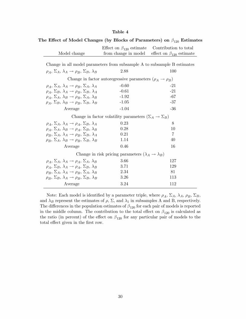
Table 4
The E¤ect of Model Changes (by Blocks of Parameters) on β120 Estimates
E¤ect on β120 estimate Contribution to totalModel change from change in model e¤ect on β120 estimate
Change in all model parameters from subsample A to subsample B estimatesρA, §A, λA ! ρB, §B, λB 2.88 100
Change in factor autoregressive parameters (ρA ! ρB)ρA, §A, λA ! ρB, §A, λA -0.60 -21ρA, §B, λA ! ρB, §B, λA -0.61 -21ρA, §A, λB ! ρB, §A, λB -1.92 -67ρA, §B, λB ! ρB, §B, λB -1.05 -37
Average -1.04 -36
Change in factor volatility parameters (§A ! §B)ρA, §A, λA ! ρA, §B, λA 0.23 8ρA, §A, λB ! ρA, §B, λB 0.28 10ρB, §A, λA ! ρB, §B, λA 0.21 7ρB, §A, λB ! ρB, §B, λB 1.14 40
Average 0.46 16
Change in risk pricing parameters (λA ! λB)ρA, §A, λA ! ρA, §A, λB 3.66 127ρA, §B, λA ! ρA, §B, λB 3.71 129ρB, §A, λA ! ρB, §A, λB 2.34 81ρB, §B, λA ! ρB, §B, λB 3.26 113
Average 3.24 112
Note: Each model is identi…ed by a parameter triple, where ρA, §A, λA, ρB, §B,and λB represent the estimates of ρ, §, and λ1 in subsamples A and B, respectively.The di¤erences in the population estimates of β120 for each pair of models is reportedin the middle column. The contribution to the total e¤ect on β120 is calculated asthe ratio (in percent) of the e¤ect on β120 for any particular pair of models to thetotal e¤ect given in the …rst row.
30
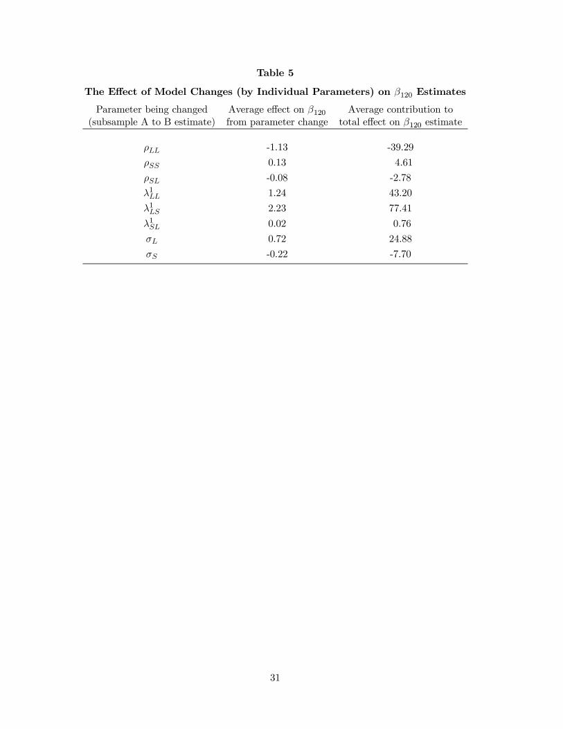
Table 5
The E¤ect of Model Changes (by Individual Parameters) on β120 Estimates
Parameter being changed Average e¤ect on β120 Average contribution to(subsample A to B estimate) from parameter change total e¤ect on β120 estimate
ρLL -1.13 -39.29ρSS 0.13 4.61ρSL -0.08 -2.78λ1
LL 1.24 43.20λ1
LS 2.23 77.41λ1
SL 0.02 0.76σL 0.72 24.88σS -0.22 -7.70
31
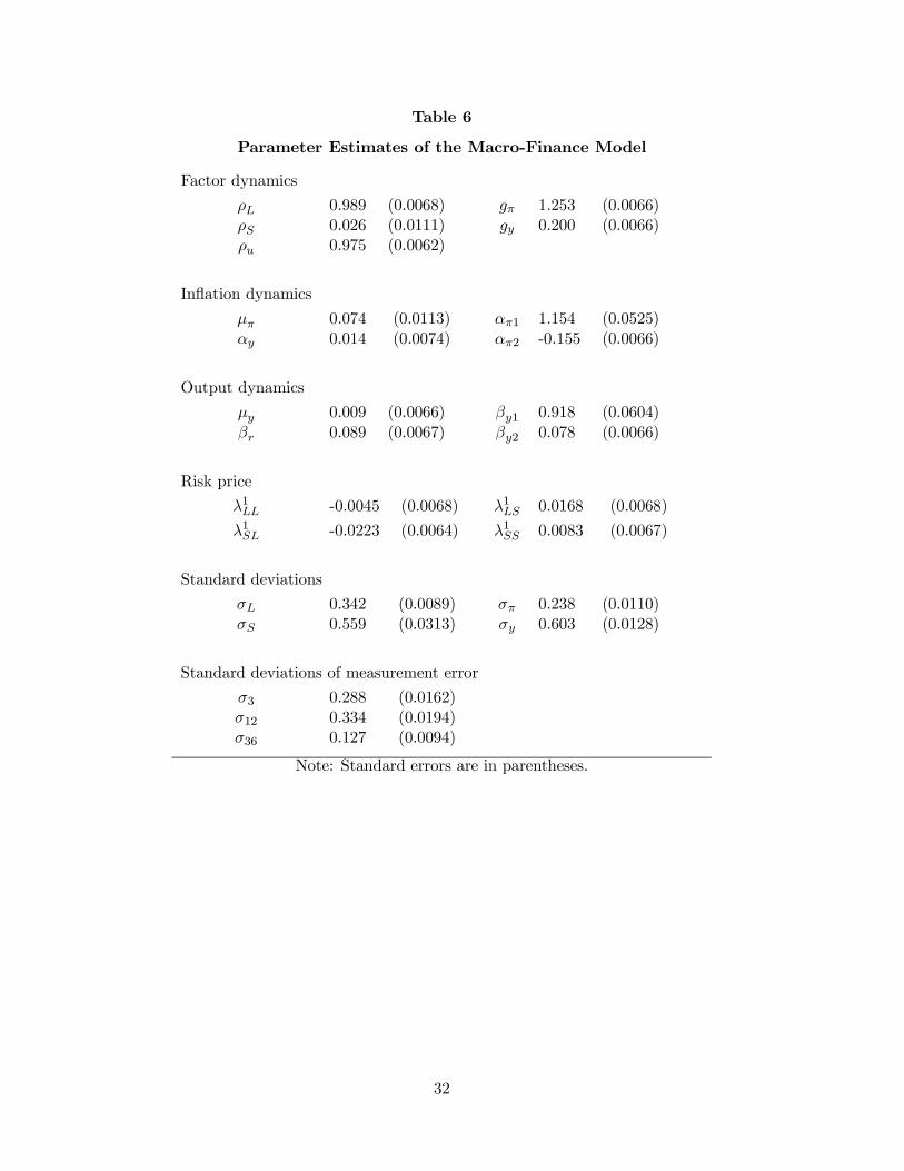
Table 6
Parameter Estimates of the Macro-Finance Model
Factor dynamicsρL 0.989 (0.0068) gπ 1.253 (0.0066)ρS 0.026 (0.0111) gy 0.200 (0.0066)ρu 0.975 (0.0062)
In‡ation dynamicsµπ 0.074 (0.0113) απ1 1.154 (0.0525)αy 0.014 (0.0074) απ2 -0.155 (0.0066)
Output dynamicsµy 0.009 (0.0066) βy1 0.918 (0.0604)βr 0.089 (0.0067) βy2 0.078 (0.0066)
Risk priceλ1
LL -0.0045 (0.0068) λ1LS 0.0168 (0.0068)
λ1SL -0.0223 (0.0064) λ1
SS 0.0083 (0.0067)
Standard deviationsσL 0.342 (0.0089) σπ 0.238 (0.0110)σS 0.559 (0.0313) σy 0.603 (0.0128)
Standard deviations of measurement errorσ3 0.288 (0.0162)σ12 0.334 (0.0194)σ36 0.127 (0.0094)
Note: Standard errors are in parentheses.
32
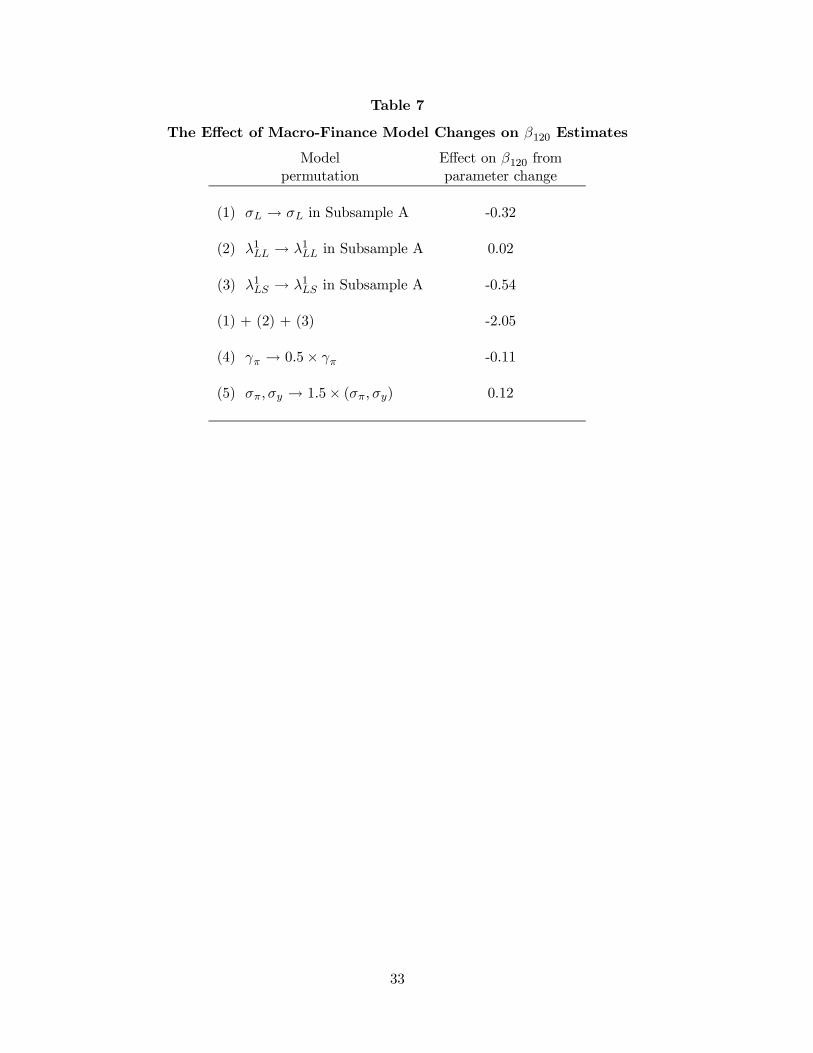
Table 7
The E¤ect of Macro-Finance Model Changes on β120 Estimates
Model E¤ect on β120 frompermutation parameter change
(1) σL ! σL in Subsample A -0.32
(2) λ1LL ! λ1
LL in Subsample A 0.02
(3) λ1LS ! λ1
LS in Subsample A -0.54
(1) + (2) + (3) -2.05
(4) γπ ! 0.5 £ γπ -0.11
(5) σπ, σy ! 1.5 £ (σπ, σy) 0.12
33
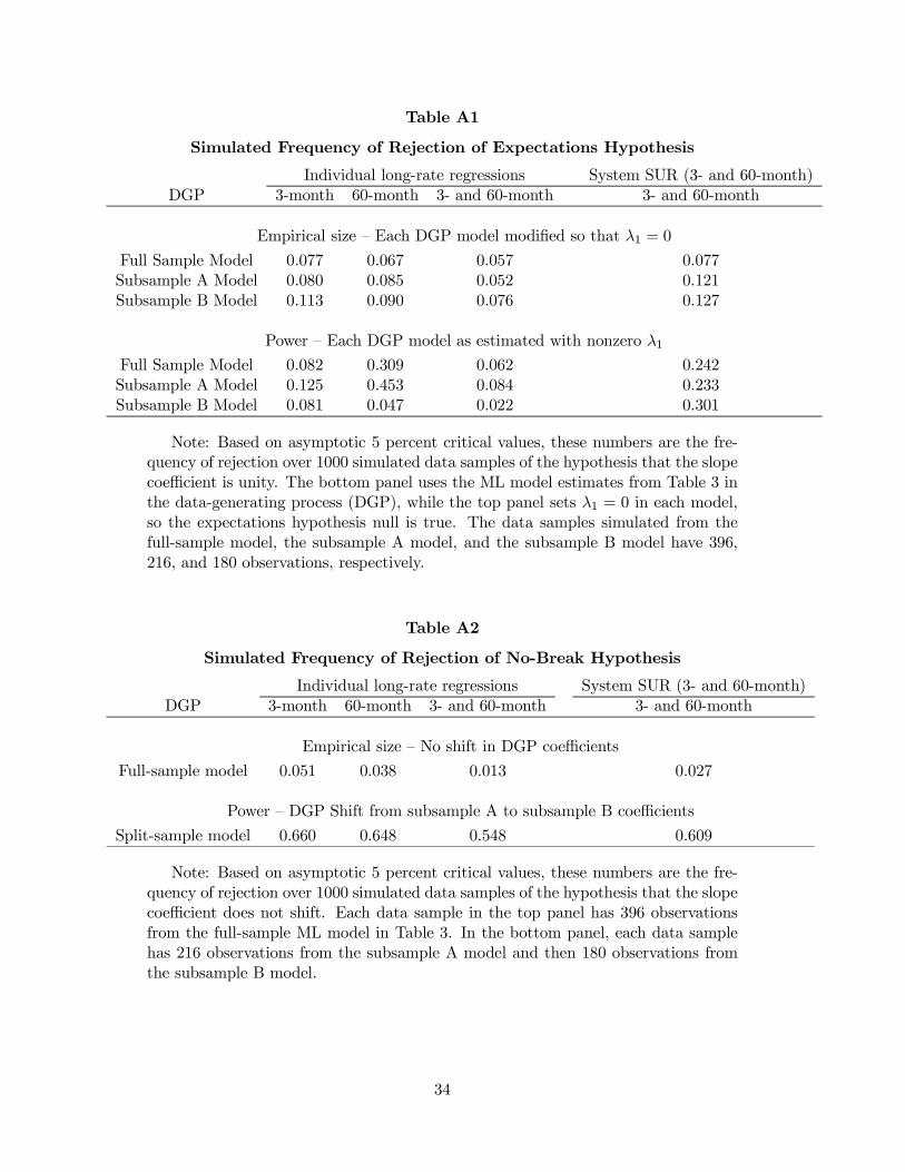
Table A1
Simulated Frequency of Rejection of Expectations Hypothesis
Individual long-rate regressions System SUR (3- and 60-month)DGP 3-month 60-month 3- and 60-month 3- and 60-month
Empirical size – Each DGP model modi…ed so that λ1 = 0Full Sample Model 0.077 0.067 0.057 0.077Subsample A Model 0.080 0.085 0.052 0.121Subsample B Model 0.113 0.090 0.076 0.127
Power – Each DGP model as estimated with nonzero λ1
Full Sample Model 0.082 0.309 0.062 0.242Subsample A Model 0.125 0.453 0.084 0.233Subsample B Model 0.081 0.047 0.022 0.301
Note: Based on asymptotic 5 percent critical values, these numbers are the fre-quency of rejection over 1000 simulated data samples of the hypothesis that the slopecoe¢cient is unity. The bottom panel uses the ML model estimates from Table 3 inthe data-generating process (DGP), while the top panel sets λ1 = 0 in each model,so the expectations hypothesis null is true. The data samples simulated from thefull-sample model, the subsample A model, and the subsample B model have 396,216, and 180 observations, respectively.
Table A2
Simulated Frequency of Rejection of No-Break Hypothesis
Individual long-rate regressions System SUR (3- and 60-month)DGP 3-month 60-month 3- and 60-month 3- and 60-month
Empirical size – No shift in DGP coe¢cientsFull-sample model 0.051 0.038 0.013 0.027
Power – DGP Shift from subsample A to subsample B coe¢cientsSplit-sample model 0.660 0.648 0.548 0.609
Note: Based on asymptotic 5 percent critical values, these numbers are the fre-quency of rejection over 1000 simulated data samples of the hypothesis that the slopecoe¢cient does not shift. Each data sample in the top panel has 396 observationsfrom the full-sample ML model in Table 3. In the bottom panel, each data samplehas 216 observations from the subsample A model and then 180 observations fromthe subsample B model.
34

0 20 40 60 80 100 120Maturity of long rate in months
-12
-10
-8
-6
-4
-2
0
2
4
Figure 1Estimated Coefficients from Long-Rate Regressions
Subsample A (1970-1987) Coefficients ± 2 std errorsSubsample B (1988-2002) Coefficients ± 2 std errors
1973 1976 1979 1982 1985 1988 1991 1994 1997 2000Range of possible breakdates
0
2
4
6
8
10
12
14
Figure 2Break Test Statistic Sequence and 5% Critical Values
5% critical valuefor unknown breakdate
5% critical valuefor known breakdate
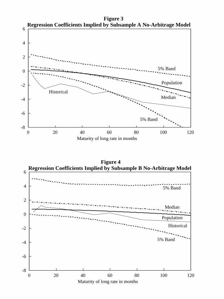
0 20 40 60 80 100 120Maturity of long rate in months
-8
-6
-4
-2
0
2
4
6
Median
Population
Figure 3Regression Coefficients Implied by Subsample A No-Arbitrage Model
Historical
5% Band
5% Band
0 20 40 60 80 100 120Maturity of long rate in months
-8
-6
-4
-2
0
2
4
6
Figure 4Regression Coefficients Implied by Subsample B No-Arbitrage Model
Population
Historical
Median
5% Band
5% Band
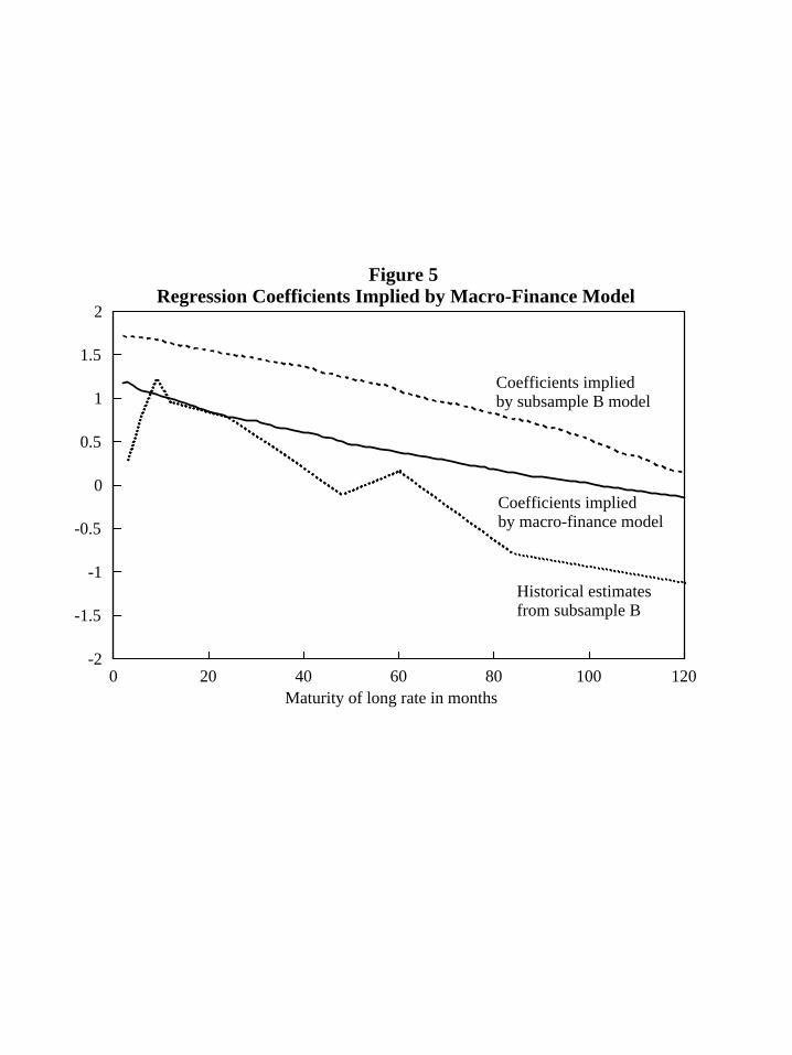
0 20 40 60 80 100 120Maturity of long rate in months
-2
-1.5
-1
-0.5
0
0.5
1
1.5
2
Coefficients implied by macro-finance model
Figure 5 Regression Coefficients Implied by Macro-Finance Model
Historical estimatesfrom subsample B
Coefficients implied by subsample B model