1

The Relationship Between Capital Structure And

Corporate Performance Under the Recent Financial

Crisis

- An Empirical Study on Listed Swedish Companies

Bachelor Thesis in Economics

Authors: Xue Feng 199203012860

Shuai Ma 198810047285

Supervisors: Professor Andreas Stephan

Jönköping May 2013

2

Contents 1 Introduction ................................................................................................................. 1

1.1 Background .............................................................................................................. 1

1.2 Problem Description and Background ........................................................................ 2

1.2.1 Research Questions .................................................................................................................. 3

1.2 Purpose ..................................................................................................................... 3

1.4 Delimitation ............................................................................................................... 3

2 Theoretical Framework ................................................................................................ 4

2.1 M&M Theory .............................................................................................................. 4

2.1.1 Modigliani-Miller Proposition with prefect capital markets ........................................... 4

2.1.2 Modigliani-Miller Proposition with Tax .............................................................................. 5

2.2 Trade-off Theory .......................................................................................................... 7

2.2.1 Interest Tax Shield (tax Benefit of Debt)) ............................................................................. 7

2.2.2 Costs of Financial Distress....................................................................................................... 8

2.2.3 Core Conception ....................................................................................................................... 9

2.3 Pecking-order Theory ................................................................................................ 11

2.3.1 Asymmetric Information ......................................................................................................... 11

2.3.2 Agency Cost .............................................................................................................................. 11

2.3.2 Core Conception ...................................................................................................................... 11

3 Earlier Studies on Determinants Of Capital Strucuture ............................................ 13

3.1 The relationship between financial distress and firm performance during the Asian

financial crisis of 1997-1998.............................................................................................. 13

3.2 Capital structure and firm performance: evidence from selected business companies

in Colombo stock exchange Sri Lanka ........................................................................... 14

4 Research Method ........................................................................................................ 15

4.1 Approach ................................................................................................................... 15

4.1.1 Quantitative Analysis ............................................................................................................. 15

4.1.2 Qualitative Analysis ............................................................................................................... 16

4.2 Data Collection ......................................................................................................... 16

4.3 Regression Model ...................................................................................................... 17

4.3.1 Goodness of Fit Statistics ....................................................................................................... 18

4.3.2 VIF (Variance Inflation Factor) ............................................................................................. 18

4.4 Analysis Of Variance (ANOVA Model) ..................................................................... 19

5. Data and Variables .......................................................................................................... 20

5.1 Dependent Variable .................................................................................................. 20

5.2 Independent Variables .............................................................................................. 21

5.2.1 Profitability ............................................................................................................................... 21

5.2.2 Uniqueness or Growth ............................................................................................................ 21

5.2.3 Cash flow/operating revenue: ................................................................................................ 22

5.2.4 Net Asset turnover ................................................................................................................... 22

5.3 Dummy Variables ...................................................................................................... 22

3

5.3.1 Model 1 ...................................................................................................................................... 23

5.3.2 Model 2 ...................................................................................................................................... 23

6 Empirical Result and Data Analysis ......................................................................... 24

6.1 Descriptive Statistics .................................................................................................. 24

6.2 Correlation ................................................................................................................. 25

6.3 Regression Analysis ................................................................................................... 26

6.3.1 Hypothesis Tests....................................................................................................................... 26

6.3.4 Interpretations of Dummy Variables ..................................................................................... 28

6.3.2 Goodness of Fit Statistics ....................................................................................................... 30

6.3.3 ANOVA Analysis ..................................................................................................................... 31

7 Concluding Remarks .................................................................................................. 33

7.1 Answer to Research Questions .................................................................................. 33

7.2 Future Research Recommendation ........................................................................... 35

8 Appendix 1_ Names of Listed 54 Swedish Company ...................................................... 36

9 Appendix 2_Equation ........................................................................................................ 2

9.1 Pearson correlation coefficient .................................................................................... 2

9.2 R-Square ....................................................................................................................... 2

9.3 Adjusted R-Square ....................................................................................................... 2

9.4 Variance Inflation Factor ............................................................................................. 2

9.5 Long-term debt ratio .................................................................................................... 2

9.6 ROA ............................................................................................................................. 2

9.7 Gross Margin ............................................................................................................... 2

9.8 Uniqueness .................................................................................................................. 3

9.9 Cash Flow/Operating Revenue Ratio ......................................................................... 3

9.10 Assest Turnover .......................................................................................................... 3

10 References ......................................................................................................................... 4

4

Figures Figure 1 MM theory without tax-proposition II _________________________________________________ 5 Figure 2 MM theory with tax-proposition I _____________________________________________________ 6 Figure 3 MM theory with tax-proposition II ____________________________________________________ 6 Figure 4: Static Trade-Off Theory_1___________________________________________________________ 7 Figure 5: The Trade-off Theory_2 ___________________________________________________________ 10 Figure 6: Pecking Order Theory _____________________________________________________________ 12

Figure 7: The tendency of each variable from 2006 to 2011 _____________________ Error! Bookmark not defined. Figure 8 Leverage Ratio Tendencies ______________________________________ Error! Bookmark not defined.

Tables Table 1: Summary Descriptive Statistics ___________________________________ Error! Bookmark not defined. Table 2: Pearson Correlation Matrix among the Variables _____________________ Error! Bookmark not defined. Table 3: Output for Regression Analysis_Model 1 ___________________________ Error! Bookmark not defined.

Table 4: Output for Regression Analysis_ Model 2 ___________________________ Error! Bookmark not defined. Table 5: Collinearity Statistics_ Model 1 ___________________________________ Error! Bookmark not defined.

Table 6: Collinearity Statistics_ Model 2 ___________________________________ Error! Bookmark not defined. Table 7: ANOVAb_ Model 1 _____________________________________________ Error! Bookmark not defined.

Table 7: ANOVAb_ Model 2 _____________________________________________ Error! Bookmark not defined.

5

Abstract

Background: In the past four decades, the relationship between capital structure and corporate

value has been extensively investigated. Sweden is ranked as one of the European countries

that have survived the financial crisis of 2007-2008 best even though the crisis affected the

economy in Sweden. Since there are few studies that discuss Swedish companies regarding

the relationship between capital structure and corporate performance, this thesis tries to find

out what is the evidence regarding Swedish companies is.

Purpose: The objective of this thesis is to describe and analyze the relationship between

capital structure and corporation performance in the listed Swedish companies under the

financial crisis. Profitability, Uniqueness or Growth, Asset composition, Cash flow/Operating

Revenue, and Net Asset Turnover are used to explore the extent to which corporate

performance influences the leverage ratio. Furthermore, this study also aims to indicate how

the financial crisis has affected the leverage ratio.

Method: This thesis is mainly a quantitative study of the relationship between capital structure

and corporate performance in listed Swedish companies under the recent financial crisis. The

quantitative study uses a regression model to illustrate this relationship and furthermore

applies statistical tests, such as ANOVA-test, to conclude whether corporate performance has

an impact on capital structure.

Conclusion: This study finds a significantly negative relationship between capital structure

and corporate performance in listed Swedish companies under the recent financial crisis in

general. Further, employing dummy variables to model the effects in various years, we find

that the leverage ratio increases before the recent financial crisis and turns to decline for three

years till the button level of capital structure. Then, it increases to the normal level.

Number of Pages in PDF File: 36

Keywords: Capital Structure, Corporation Performance, Leverage, Corporate Finance,

Recent Financial Crisis, Swedish Companies.

JEL Classification: G32

1

1 Introduction

In the following section, the thesis starts with a brief description of the recent Financial

Crisis. Then it is followed by a discussion about capital structure, which a large amount of

scholars have studied in the past four decades. At the end, the main purpose of the thesis and

the limitation are described.

1.1 Background

The collapse of Lehman Brothers in 2008 caused a global meltdown in the financial market.

The stock markets of the world fell and large financial institutions fail (Shah, 2013). Banks

stopped to lend to each other (McKibbin & Stoeckel, 2009). The amount of debt in firm

capital structures increased, the capital and lending markets collapsed (Fosberg, 2004). Many

economists point out that the recent financial crisis is the worst crisis since the great

depression of 1930s (Business Wire News database, 2009).

Owing to Sweden’s highly dependence on the outside world, the international economic

downturn had a substantial impact on the economy of Sweden (Öberg, 2009). Financial

shocks had a negative impact on real GDP growth, and GDP in Sweden decreased by 4.9

percent during the recent financial crisis. In addition, the Swedish stock market fell by more

than 40 percent and the leverage of firms in Sweden declined extremely (Österholm, 2010).

The reason why the authors of the thesis analyse Swedish firms is based on the following

reasons: First, Sweden remains highly integrated into the global economy with strong trade

and investment activity, thus the dependence of Sweden on the global economy is significant

(Ketels, 2012). Secondly, according to Servcorp International Business Confidence survey

(2009), it is illustrated that Sweden is ranked as one of the European countries that have

survived the financial crisis of 2007-2008 best .The capital structure of Swedish firms is of

great interest since Sweden has managed the recent financial crisis successfully (Johanson,

2009). Lastly, there are few researches that discuss the company performance and financial

crisis at same time for Swedish corporations. This thesis aims to fill this gap.

2

1.2 Problem Description and Background

Capital structure decision is the mix of debt and equity that a company uses to finance its

business (Damodaran, 2001). The relationship between capital structure and corporate

performance has been extensively investigated in the past four decades.

Gleason et al. (2000) indicate that managers make use of different debt ratio, which is also

called leverage ratio, as a firm-specific strategy to improve the performance of the company.

Under this strategy, the majority of the firms attempt to attain an optimal leverage ratio so that

they can both maximize the firm value and minimize the cost of capital and risk. In other

words, the optimal leverage ratio promotes the company’s competitive advantage in the

capital market.

Rajan and Zingales (1994) suggest that the capital structure has diverse national patterns.

Several studies have investigated this for some European countries and the US. Moreover,

Gleason et al. (2000) reveal that there is a negative relationship between capital structure and

corporation performance in European countries, while Roden and Lewellen (1995) illustrate

that there is a significant positive relationship between capital structure and corporation

performance in the US. Here are obviously contradictory results in different countries and

there is lack of similar research done in Sweden.

After going through the theoretical literature, the authors of this thesis found that the

relationship between capital structure and corporate performance is a quite interesting topic to

investigate and it would be better to target the analysis only in one specific country. Since

Sweden has not intensively been explored on this topic before, it would be unique and is a

challenge to find out what the conclusion regarding Swedish companies are.

From this view, the thesis intends to study a sample of Swedish companies. Moreover, since

the recent financial crisis has influenced the European economics a lot, it may have given a

shock to Swedish companies’ capital structure as well. This thesis tries to investigate how the

recent financial crisis influences the relationship between capital structure and corporate

performance, and explores the extent to which corporate performance influences the leverage

ratio. Additionally, it measures firm performance using various indicators: Profitability,

Uniqueness or Growth, Asset composition, Cash flow/operating revenue, and Net Asset

Turnover, since they might have different effects on capital structure. Based on the data the

authors have, it will show what the adjustment of capital structure due to the recent Financial

Crisis in listed Swedish companies was.

3

1.2.1 Research Questions

The thesis tries to answer the following main research question:

What is the relationship between capital structure and corporation performance for

listed Swedish companies under the recent financial crisis?

Sub-research question 1: What are the determinants of the corporation performance?

Sub-research question 2: What is the relationship between each determinant and the capital

structure?

Sub-research question 3: What is the debt ratio tendency before and after the financial crisis

in the Swedish companies?

1.2 Purpose

This research is trying to illustrate a general description of the relationship between capital

structure and corporation performance in the listed Swedish companies under the financial

crisis, and also indicates how the financial crisis affects the leverage ratio. Some suggestions

will be given to further research in the same field. The purpose is to get convincing and

meaningful results, which would help the financial manager to make appropriate adjustment

on the company’s capital structure.

1.4 Delimitation

Firstly, our main limitation is data collection. In the beginning, the authors intended to

investigate the top 250 companies in Sweden from the Amadeus website, a database

providing comparable financial information for public and private companies across Europe.

However, while the authors planned to collect primary data of TOP 250, the majority of

Swedish companies’ data is not available. Moreover, the authors could not find comparable

data from other databases. After deleting companies with the incomplete data, the authors

only got a sample of 54 companies.

Secondly, in the regression model, no results are provided according to industry category.

Since the leverage ratio is affected by industry pattern, it may distort the results from the

regression model.

Thirdly, there are five independent variables in the regression model. It is not fully clear if

more meaningful results could be obtained by adding more control variables to the model.

4

2 Theoretical Framework

In this chapter, major theories concerning capital structure will be described. It starts with a

brief introduction of the ‘irrelevant’ capital structure theory: M&M Theory. This theory is

the origin of all modern capital structure theory. Even though the main assumption of this

theory is a perfect capital market, which is not applicable to real economic issues, it plays a

significant role in the history of the capital structure theory. Then it is followed by the

introduction and deep discussion of two other major theories: Trade-off Theory and Pecking-

order Theory.

2.1 M&M Theory

2.1.1 Modigliani-Miller Proposition with prefect capital markets

Miller and Modigliani (1958) primarily developed the capital structure theorem in a seminal

article published in the American Economic Review. They find that a firm’s value is not

dependent upon their capital structure in efficient markets, it does not matter what capital

structure a firm uses to finance its operations. Therefore, Miller and Modigliani developed

two hypotheses under the perfect capital market.

Proposition I

“Market value of any firm is independent of its capital structure” (Miller & Modigliani,

1958). Even though changing the proportions of capital structure in a firm, the total values of

its outstanding securities remain the same (Ross et al., 2011). According to the equation

VU=VL, where Vu is the value of an unlevered firm value and VL is the value of a levered

firm, which illustrates that whether a firm has no debt or a company that funds its operations

by taking out loans, the two corporation values are identical.

Proposition II

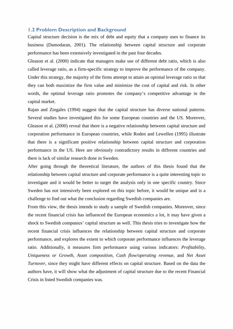
“The cost of equity is positively related to leverage”. It demonstrates that the positive

relationship between the proportion of debt in capital structure of a firm and its return on

equity to shareholders (Miller & Modigliani, 1958). This is related to the formula 𝑟𝑊𝐴𝐶𝐶 =

𝐸

𝐸+𝐷∗ 𝑟𝐸 +

𝐸

𝐸+𝐷∗ 𝑟𝐷, Where 𝑟𝑊𝐴𝐶𝐶 is weighted average cost of capital, 𝑟𝐸 is cost of equity, 𝑟𝐷

is cost of debt, D is market value of firm’s debt and E is equity of shareholder (Kootanaee et

al, 2012). Corporations are typically financed by a combination of debt and equity. The

weighted average cost of capital weights the cost of equity and the cost of debt by the

percentage of each used in a firm’s capital structure. Increasing leverage makes more risky for

5

the equity holder so that the cost of equity must increase, thus the leverage is positively

related to the required return on equity. Below a graph is shown where the horizontal line

represents the debt to equity ratio (D/E) and the vertical line represents the cost of capital. As

debt to equity ratio grows, the return to equity rises; Expected return of the unlevered firm's

equity is independent of leverage. The value of unlevered firm equals the weighted average

cost of capital. Thus the weighted average cost of capital (WACC) remains constant (Stanton

& Seasholes, 2005).

𝑟𝐸

𝑟𝑊𝐴𝐶𝐶

𝑟𝐷

Figure 1 MM theory without tax-proposition II

Source: Berk & DeMarzo (2007), authors’ own illustration

2.1.2 Modigliani-Miller Proposition with Tax

However, Miller and Modigliani propositions were based on the restrictive assumption of no

tax, bankrupt cost and agency costs (Hillier et al., 2010) and this assumption is inconsistent

with the real world since there is no perfect capital market with no tax, transaction cost and

other costs. According to Campello (2006), firms generally employ only moderate amounts of

debt. After that, Miller and Modigliani (1963) modified their existent propositions and created

new hypotheses about tax benefits as determinant of capital structure. According to Miller

(1977), the value of firms depends on the relative level of each tax rate.

Proposition I

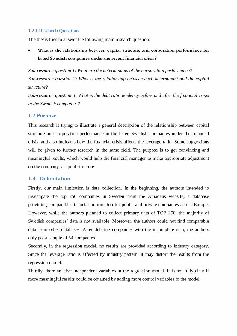
Due to the present value of interest payments from corporate-tax liabilities, the value of the

firm with leverage firm exceeds the value of the unlevered firm. The graph illustrates a

straight line with a slope of Tc gives the relationship between the value of firm and total debt.

The present value of tax shield is the distance between the two lines. Through the equation VL

=Vu + Tc* D, where Tc* D is the present value of the interest tax shield, the value of levered

firm is larger than that of unlevered firm when taking tax into consideration. Baumol and

Cost of Capital

Debt/Equity Ratio

𝑟𝑢

6

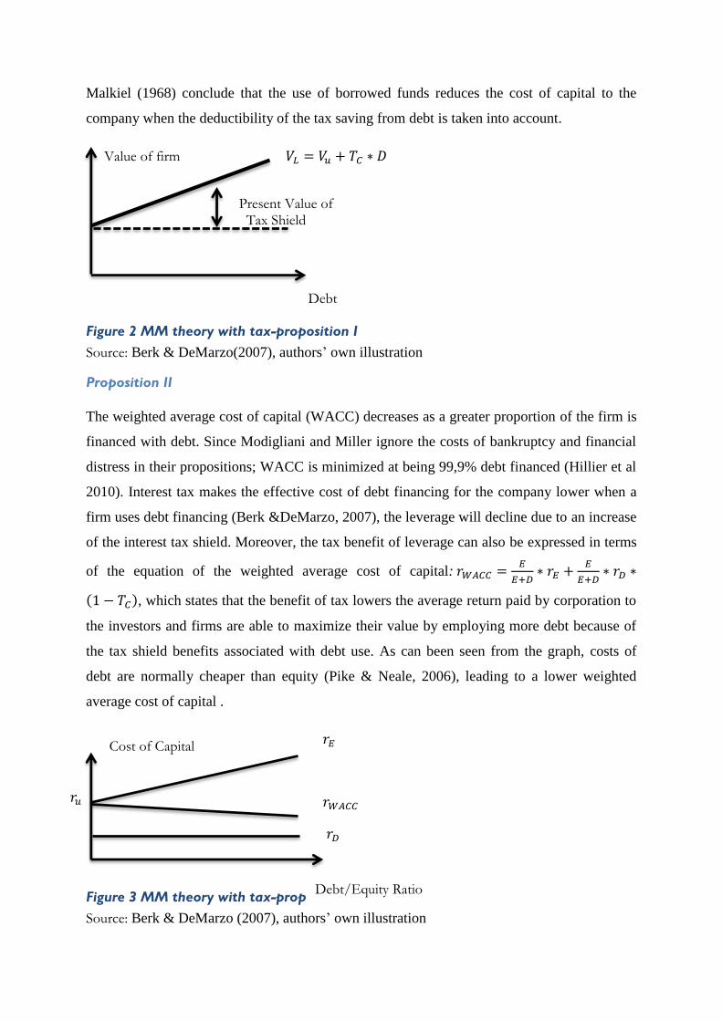
Malkiel (1968) conclude that the use of borrowed funds reduces the cost of capital to the

company when the deductibility of the tax saving from debt is taken into account.

Value of firm 𝑉𝐿 = 𝑉𝑢 + 𝑇𝐶 ∗ 𝐷

Present Value of Tax Shield

Debt

Figure 2 MM theory with tax-proposition I

Source: Berk & DeMarzo(2007), authors’ own illustration

Proposition II

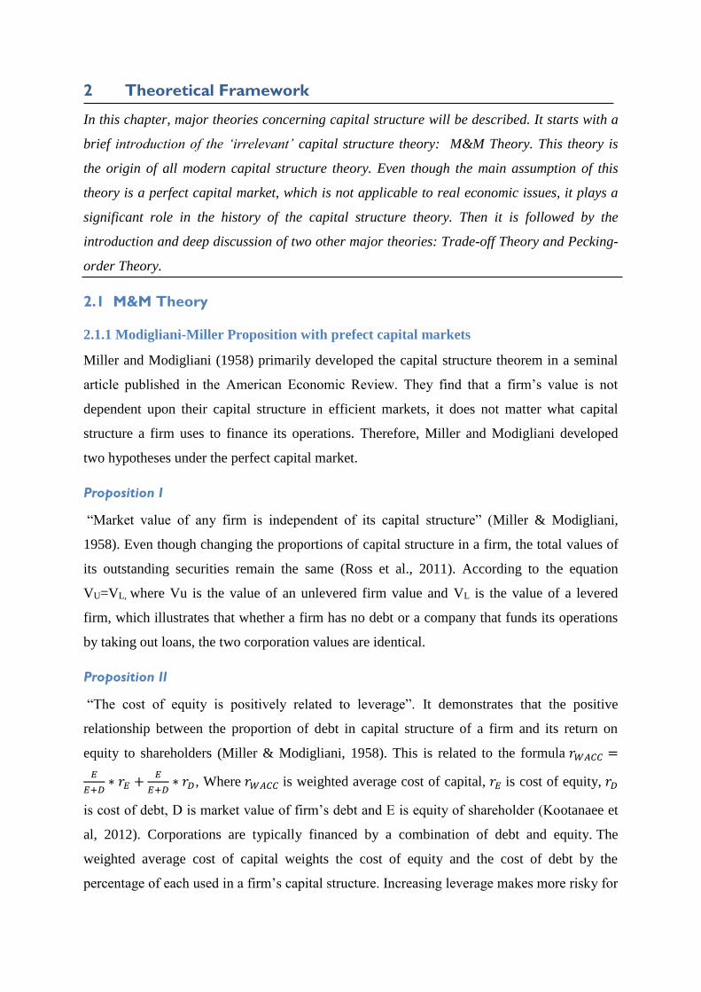
The weighted average cost of capital (WACC) decreases as a greater proportion of the firm is

financed with debt. Since Modigliani and Miller ignore the costs of bankruptcy and financial

distress in their propositions; WACC is minimized at being 99,9% debt financed (Hillier et al

2010). Interest tax makes the effective cost of debt financing for the company lower when a

firm uses debt financing (Berk &DeMarzo, 2007), the leverage will decline due to an increase

of the interest tax shield. Moreover, the tax benefit of leverage can also be expressed in terms

of the equation of the weighted average cost of capital: 𝑟𝑊𝐴𝐶𝐶 =𝐸

𝐸+𝐷∗ 𝑟𝐸 +

𝐸

𝐸+𝐷∗ 𝑟𝐷 ∗

(1 − 𝑇𝐶), which states that the benefit of tax lowers the average return paid by corporation to

the investors and firms are able to maximize their value by employing more debt because of

the tax shield benefits associated with debt use. As can been seen from the graph, costs of

debt are normally cheaper than equity (Pike & Neale, 2006), leading to a lower weighted

average cost of capital .

𝑟𝐸

𝑟𝑊𝐴𝐶𝐶

𝑟𝐷

Figure 3 MM theory with tax-proposition II

Source: Berk & DeMarzo (2007), authors’ own illustration

Cost of Capital

Debt/Equity Ratio

𝑟𝑢

7

If capital structure is irrelevant in a perfect market (M&M Theory), then imperfections, which

exist in the real world, must be the cause of its relevance. The theories below try to address

some of these imperfections, relaxing assumptions made in the M&M model.

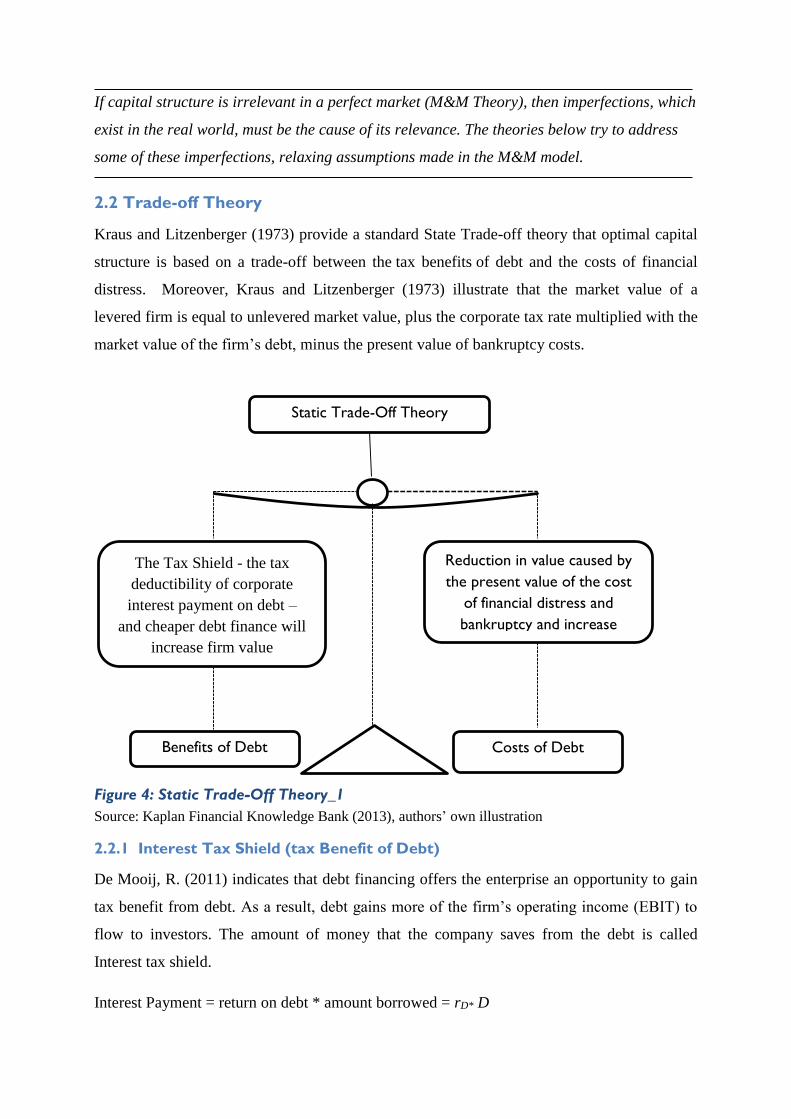
2.2 Trade-off Theory

Kraus and Litzenberger (1973) provide a standard State Trade-off theory that optimal capital

structure is based on a trade-off between the tax benefits of debt and the costs of financial

distress. Moreover, Kraus and Litzenberger (1973) illustrate that the market value of a

levered firm is equal to unlevered market value, plus the corporate tax rate multiplied with the

market value of the firm’s debt, minus the present value of bankruptcy costs.

Figure 4: Static Trade-Off Theory_1

Source: Kaplan Financial Knowledge Bank (2013), authors’ own illustration

2.2.1 Interest Tax Shield (tax Benefit of Debt))

De Mooij, R. (2011) indicates that debt financing offers the enterprise an opportunity to gain

tax benefit from debt. As a result, debt gains more of the firm’s operating income (EBIT) to

flow to investors. The amount of money that the company saves from the debt is called

Interest tax shield.

Interest Payment = return on debt * amount borrowed = rD* D

Static Trade-Off Theory

The Tax Shield - the tax

deductibility of corporate

interest payment on debt –

and cheaper debt finance will

increase firm value

Reduction in value caused by

the present value of the cost

of financial distress and

bankruptcy and increase

agency costs

Benefits of Debt Costs of Debt

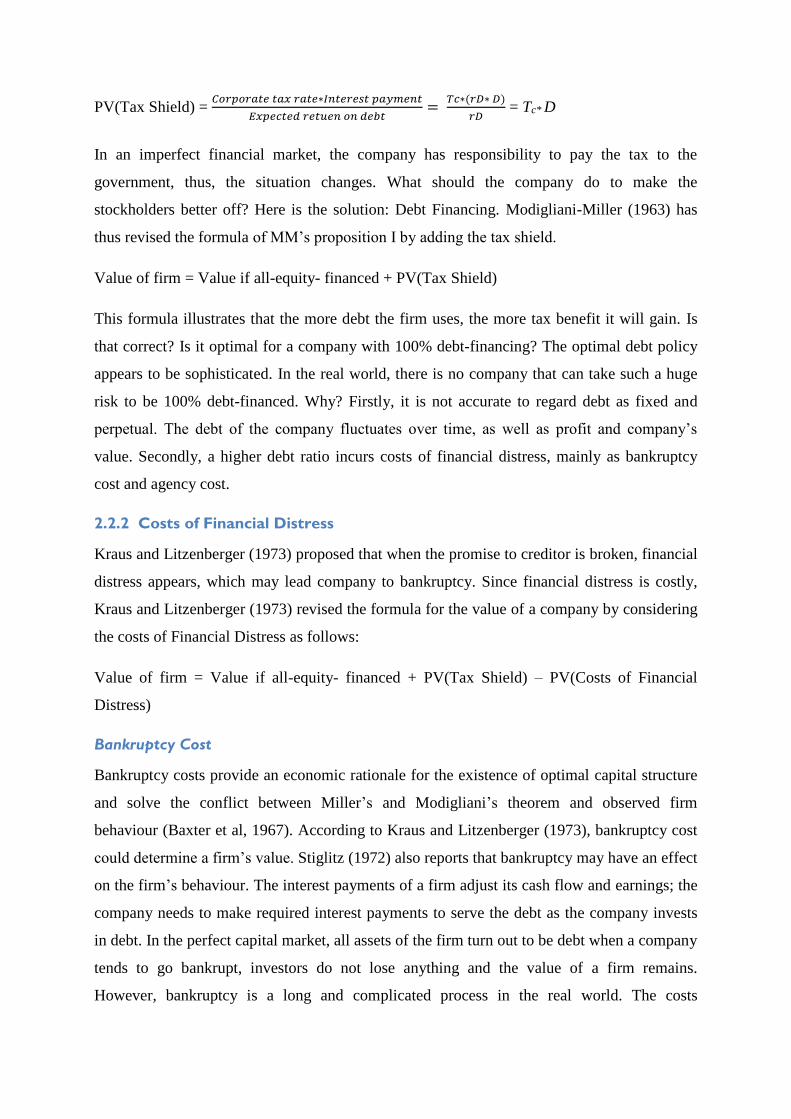
8

PV(Tax Shield) = 𝐶𝑜𝑟𝑝𝑜𝑟𝑎𝑡𝑒 𝑡𝑎𝑥 𝑟𝑎𝑡𝑒∗𝐼𝑛𝑡𝑒𝑟𝑒𝑠𝑡 𝑝𝑎𝑦𝑚𝑒𝑛𝑡

𝐸𝑥𝑝𝑒𝑐𝑡𝑒𝑑 𝑟𝑒𝑡𝑢𝑒𝑛 𝑜𝑛 𝑑𝑒𝑏𝑡=

𝑇𝑐∗(𝑟𝐷∗ 𝐷)

𝑟𝐷 = Tc* D

In an imperfect financial market, the company has responsibility to pay the tax to the

government, thus, the situation changes. What should the company do to make the

stockholders better off? Here is the solution: Debt Financing. Modigliani-Miller (1963) has

thus revised the formula of MM’s proposition I by adding the tax shield.

Value of firm = Value if all-equity- financed + PV(Tax Shield)

This formula illustrates that the more debt the firm uses, the more tax benefit it will gain. Is

that correct? Is it optimal for a company with 100% debt-financing? The optimal debt policy

appears to be sophisticated. In the real world, there is no company that can take such a huge

risk to be 100% debt-financed. Why? Firstly, it is not accurate to regard debt as fixed and

perpetual. The debt of the company fluctuates over time, as well as profit and company’s

value. Secondly, a higher debt ratio incurs costs of financial distress, mainly as bankruptcy

cost and agency cost.

2.2.2 Costs of Financial Distress

Kraus and Litzenberger (1973) proposed that when the promise to creditor is broken, financial

distress appears, which may lead company to bankruptcy. Since financial distress is costly,

Kraus and Litzenberger (1973) revised the formula for the value of a company by considering

the costs of Financial Distress as follows:

Value of firm = Value if all-equity- financed + PV(Tax Shield) – PV(Costs of Financial

Distress)

Bankruptcy Cost

Bankruptcy costs provide an economic rationale for the existence of optimal capital structure

and solve the conflict between Miller’s and Modigliani’s theorem and observed firm

behaviour (Baxter et al, 1967). According to Kraus and Litzenberger (1973), bankruptcy cost

could determine a firm’s value. Stiglitz (1972) also reports that bankruptcy may have an effect

on the firm’s behaviour. The interest payments of a firm adjust its cash flow and earnings; the

company needs to make required interest payments to serve the debt as the company invests

in debt. In the perfect capital market, all assets of the firm turn out to be debt when a company

tends to go bankrupt, investors do not lose anything and the value of a firm remains.

However, bankruptcy is a long and complicated process in the real world. The costs

9

associated with financial distress consist of direct and indirect cost. When a firm tends to hold

more leverage, bankruptcy becomes more risky to credit holder, the payment to debt holder

will decline and debt holder cannot get what they own, which leads to the balance between tax

benefit and the equity changes (Baxter, 1967). Warner (1977) notes that distinguishing two

kinds of costs are of significance. Direct costs are out of pocket cash expense such as legal

and administrative cost; it is usually lower when the total value available to all investors.

Megginson & Smart (2008) indicate that the amounts of direct cost are much smaller than that

of pre-bankruptcy market value of large firms, so it is to small to discourage use of debt

financing.

Financial distress indirect cost incurred in the process which a firm spends resources to avoid

the firm go bankrupt. The incremental losses of financial distress and losses associated with

the total value of the firm play a significance role in identifying the indirect cost. Losses of

customers and of suppliers are examples of indirect bankruptcy costs. The indirect costs

associated with financial distress are usually larger than direct bankrupt cost and are hard to

measure correctly (Warner, 1977). Moreover, Warner (1977) points out that if the indirect

bankruptcy cost is important, it is necessary to seek an optimal capital structure so that more

value for the firm created.

2.2.3 Core Conception

Under the assumption of the possibility of bankruptcy, Kraus and Litzenberger (1973) suggest

that the company with optimal debt ratio has a maximium maket value by the trade-off

between tax benefit from debt financing and the cost of financial distress.

Kraus and Litzenberger (1973) indicate that the firm’s financing mix determines the states in

which the firm will earn its debt obligation and receive the tax savings attributable to debt

financing, if the companies’ debt obligation exceeds its revenue, the market value cannot be

positively affected by the debt obligation.

At moderate debt ratios, the effect of financial distress is immaterial and the tax shield

dominates the effect on the value of the firm. But further increases of the debt ratio leads to a

decline in the marginal benefit of debt while the marginal cost of the financial distress

dominates. The theoretical optimal debt ratio is estimated to reach a level that the present

value of the tax saving due to additional borrowing is just offset by increases in the present

value of cost of distress.

10

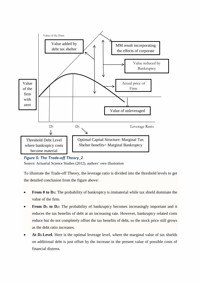
Value of the Firm

D1 D2 Leverage Ratio

Figure 5: The Trade-off Theory_2

Source: Actuarial Science Studies (2012), authors’ own illustration

To illustrate the Trade-off Theory, the leverage ratio is divided into the threshold levels to get

the detailed conclusion from the figure above:

From 0 to D1: The probability of bankruptcy is immaterial while tax shield dominate the

value of the firm.

From D1 to D2: The probability of bankruptcy becomes increasingly important and it

reduces the tax benefits of debt at an increasing rate. However, bankruptcy related costs

reduce but do not completely offset the tax benefits of debt, so the stock price still grows

as the debt ratio increases.

At D2 Level: Here is the optimal leverage level, where the marginal value of tax shields

on additional debt is just offset by the increase in the present value of possible costs of

financial distress.

Value added by

debt tax shelter

benefit

Value reduced by

Bankruptcy

MM result incorporating

the effects of corporate

Actual price of

Firm

Value of unleveraged

Firm

Value

of the

firm

with

zero

debt

Threshold Debt Level

where bankruptcy costs

become material

Optimal Capital Structure: Marginal Tax

Shelter benefits= Marginal Bankruptcy

11

After D2: The bankruptcy related costs exceed the tax benefits, so from this point on

increasing the debt ratio lowers the value of the firm.

By this theory it is assumed that the managers, stockholders and creditors receive the same

information about the company, and the price of the stocks is fairly settled by their true

underlying value. However, this situation does not exist in the real world. In fact, the

information that investors know is normally less than the managers. Under this condition, the

optimal leverage ratio cannot be only decided by the tax shield and cost of financial distress,

because the asymmetric information has to be taken into account. In the following an

alternative theory to solve this problem is presented: Pecking-order Theory.

2.3 Pecking-order Theory

2.3.1 Asymmetric Information

In real world, Berk DeMarzo (2012) states that company managers have a privilege to know

more internal financial information about the company than the outsider investors, such as the

profitability and prospect of the firm. Therefore, managers can take advantage of their

additional information and mislead the investors to believe in the wrong prospect of firm

development so that the investors may not be able to access the true value of the new

securities of the company.

Hillier (2010) discusses that investors regard the announcement of a stock issue as a signal of

change in stock price: managers issue will new stock when the stock price is over-priced,

while managers will use retained earing when the stock price is underpriced. In this way,

managers can manipulate investors by issuing a stock even though it is underpriced.

2.3.2 Agency Cost

Jensen and Meckling (1976) emphasize that asymmetric information also heads to a serious

problem: different agency costs among the various financing. Due to the asymmetric

information between internal managers and external investors, any external financing will

generate agency costs, which will reduce the value of the company. In fact, if the company is

using internal financing, this will not increase the company's agency costs.

2.3.2 Core Conception

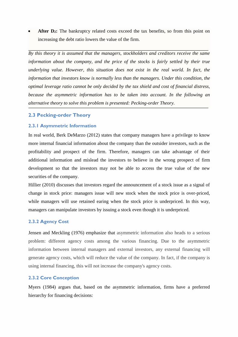
Myers (1984) argues that, based on the asymmetric information, firms have a preferred

hierarchy for financing decisions:

12

Figure 6: Pecking Order Theory

Source: Kaplan Financial Knowledge Bank (2013), authors’ own illustration

Firstly, firms prefer internal financing. The manager can totally evade any speculations, since

internal financing implies not to issue debt or equity, and the company simply transfers its

own money into investment capital, most commonly used are the retained earnings.

Secondly, if the company does not possess sufficient internal capital, the secondary option is

external financing, which is to issue debt or equity. However, there are some preferences

within this option. The company will primarily issue debt as the safer a security the better,

because debt is less risky in comparison to equity.

InternallyGernerated

FundsDebt

New Issue ofEquity

13

3 Earlier Studies on Determinants Of Capital Strucuture

In this chapter, the two empirical studies concerning the capital structure will be displayed

and discussed. One is from in Asia, and another one is from Sri Lanka. These two literatures

inspired the authors to write a paper about capital structure decisions, and provided the

knowledge of how to build the regression model for the analysis.

3.1 The relationship between financial distress and firm performance

during the Asian financial crisis of 1997-1998

The study conducted by Tan (2003) investigates the relationship between financial distress

and firm performance during the Asian financial crisis of 1997-1998.

The author of this paper uses the crisis as an exogenous shock to reduce the endogeneity

issues of the performance – leverage relationship. Owing to most of prior researches have

studied the performance–leverage relationship in the U.S. context, the purpose of this paper is

using descriptive approach to re-exam the relationship between performance and financial

crisis under an international context. Furthermore, this study aims to test whether financial

distress cost lowers the firm performance.

The data used in the study consists of 277 firms, which results in 2,216 firms-year

observations over 8 years from eight East Asian countries. The collected firms’ financial data

are retrieved from the Compustat Global database from 1993 to 2002 and have complete

financial information for the entire sample period.

In this research paper, return on assets (ROA) and Tobin’s q are used as measures for the

firm performance as a dependent variable. Leverage is measured using long-time debt ratio

(book value of the firm’s long-term debt divided by total assets) as independent variable.

Furthermore, sales, prior profitability, and prior total asset growth are control variables.

Regression analysis approach was used to assess the impact of leverage on firm performance.

The results drawn from this study are as follows: first, regressing the performance measures

on leverage and crisis, does not take any control variable into consideration, the crisis

coefficient is negative and significant, thus firms have lower performance. Moreover, firms

with high leverage perform poorly compare to firms with low leverage during the crisis.

Second, adding the size, growth opportunities, and prior profitability variables, high-

leveraged firms are still expected to underperform relative low-leveraged firm. Third, the

relationship between leverage and corporate performance is negative and is sensitive to the

14

financial crisis. It suggests that financial crisis extends the negative performance-leverage

relationship. Furthermore, Tan (2003) makes a further study on investigate whether the

performance –leverage relationship was affected by the countries’ rules and norms.

3.2 Capital structure and firm performance: evidence from selected

business companies in Colombo stock exchange Sri Lanka

Pratheepkanth (2011) has conducted a study on the relationship between capital structure and

firm performance. The author aims to study the evidence from selected business companies of

the Colombo stock exchange in Sri Lanka. The objective in this paper is to reveal the impact

of capital structure on financial performance of the listed companies traded in Colombo stock

exchange.

The data of this study was collected from Business Companies’ financial statements during

the 2005-2009. All the corporations in Sri Lanka are used which are listed on Colombo Stock

Exchange. Three hypotheses are tested in the study: The relationship between capital structure

and firm performance are negative or positive and whether the capital structure affects the

firm performance significantly.

In this research paper, Pratheepkanth (2011) chooses debt to equity ratio and debt to total

asset ratio to measure the capital structure, and four independent variables: Gross profit, Net

profit, Return on equity (ROE), Return on investment (ROI), which measure the financial

performance.

Correlation analysis and regression analysis approaches are used to evaluate the capital

structure- firm performance relationship. The result of this paper states that the capital

structure (debt to equity ratio and debt to total asset ratio) have insignificant negative impact

on Net profit, ROA, ROI, while Gross profit is negatively related to the capital structure.

Pratheepkanth (2011) finds that there is negative relationship between capital structure and

firm performance in Sri Lanka during 2005-2009. Furthermore the author discusses the

suggestions for increasing the firm’s financial performance. Performance standards will help

investors take better investment decisions; it is necessary for companies to communicate

timely with investors. In addition, inflation and exchange rate also affect the corporation

performance; therefore government should control the inflation and exchange rate.

15

4 Research Method

In this chapter, the main research method will be displayed and discussed. The authors start

with summary of the Quantitative Analysis and Qualitative Analysis and explain why only

Quantitative Analysis has been chosen in this thesis. Then, it is followed by the data

collection, which includes primary and secondary data sources, and sample selection criteria.

In the end, we explain which regression model should be used and describe analyses of

testing for multicollinearity in regression models.

4.1 Approach

4.1.1 Quantitative Analysis

Quantitative research provides the systematic empirical investigators an overview of the target

situation through statistical, mathematical or computational techniques. (Given,2008). Lafaille

and Wildeboer (1995) indicate that the selection of appropriate measurements is the crucial

part of the quantitative research, since it illustrates the fundamental relationships between

empirical observations and mathematical expression of data.

Given (2008) argues that quantitative research is extensively used in social sciences, such as

psychology, economics, sociology, marketing, and information technology. Qualitative

methods povide information only on the particular cases studied, and any more general

conclusions are only hypotheses. Quantitative methods can be used to verify which of such

hypotheses are true.

In this thesis, quantitative methods are used to analyze the relationship between capital

structure and corporation performance based on a sample of 54 listed Swedish companies

under the recent financial crisis. Firstly, measurements of capital structure and corporation

performance have been selected. Secondly, the data is collected from the Amadeus website, a

database, which provides financial and business information on a large number of European

countries. Thirdly, after primary data was selected to the secondary data that could be used, E-

views and SPSS, analytical statistical software packages, have been used to estimate the

regression model between the capital structure as dependent and corporation performance as

independent variable and to test covariance among the variables. At the end of this part,

conclusions are drawn based on the output of the regression models and futurther suggestions

are provided to the researchers who want to do the similar topics in the future.

16

4.1.2 Qualitative Analysis

Qualitative research gives the investigator a general view of situation and a deeper

understanding of social process and context. Beyond that, a qualitative method provides

investigator with more space to interpretation and gives them greater opportunity to acquire

knowledge (Morgan &Smircich, 1980). Participant observation, in-depth interviews and focus

groups are the most common qualitative methods (Morgan &Margaret, 1984).

However, some limitations exist in the qualitative approach, therefore the authors in this paper

have not chosen this method: Firstly, qualitative method does not involve measurement or

statistics, but the authors use numerical data collection for the analysis. Secondly, this

approach usually takes long time to collect data; sometimes it can last for months or even

years. Thirdly, qualitative research is only suitable for people who care about it, takes it

seriously, and is prepared for commitment (Delamont, 1992). In our case, to interview the

selected listed Swedish companies in the process of data gathering is not feasible.

4.2 Data Collection

After looking through the majority of literature about the capital structure, current financial

crisis and determinants of corporate performance, the authors gain the general idea and decide

about the appropriate independent variable and dependent variables for measuring leverage

and corporate performance in this research. Later, authors conducted the quantitative research,

based on data from the Amadeus website, a database, which provides financial and business

information on a large number of European countries.

Data selection for this study was based on certain criteria: The Region/Country: Sweden, and

the size of the firm: top 250. Initially, we got the data of TOP 250 Swedish companies, but

plenty of companies’ data is missing. After the primary data is selected and re-organized into

secondary data, the search resulted in a sample of 54 Swedish companies. The data of the

Swedish companies is from 2006 to 2010. In the end, there are 325 observations have been

recorded.

After 325 observations are analysed by the SPSS software, which is an abbreviation of

Statistical Package for the social sciences and is most widely used for analyzing data in social

sciences, the authors obtained various tables for the regression model that contribute to

quantitative analysis. The correlations between the independent variables interpret the

covariance in this regression model. The coefficient of each variable illustrates the different

relationship between dependent variables with each independent variable. The ANOVA table

17

shows the differences between group means and provides a statistical test of whether or not

the mean of several groups are equal. Based on these Tables, the hypothesis tests will be

conducted to derive the conclusions of this research paper.

4.3 Regression Model

Regression analysis is a statistical tool to investigate the relationship among

variables (Sykes, 1992). The reason for using regression method is identifying a correlation

between the studied variables. According to Aczel (1999), the regression analysis approach

focuses on study the independent variable and the degree of independent variable influence on

explanatory or dependent variable. It also evaluates the statistical significance of the estimated

relationship and provides estimations of quantitative effect of variables. When making a

multiple regression model, investigator aims to study the relationship between a dependent

variable and more than one independent variable. The regression fits the equation according

to the formula: Y=β0+β1X1 +β2X2 +β3X3 +β4X4 +β5X5 +ε

In which, X1, X2, X3, X4, X5 are independent variables, Y is dependent variable, β0 is intercept

coefficient, β1, β2, β3, β4, β5 are slope coefficients. ε is the error term, which is drawn

independently from a normal distribution with mean zero and constant variance.

The authors try to study all independent variables affect dependent variable in the multiple

regression model, the relationship between dependent variable (long-term debt ratio) and

independent variables. The two formulated regression models are shown below:

Model 1: Leverage ratio = β0 + β1 ROA + β2ln (GM) +β3 (R&D) + β4 ln (CF/OR) + β5 NAT

+ D2006+ D2007+ D2009+ D2010+ D2011 + ε

Model 2: Leverage ratio = β0 + β1 ROA + β2ln (GM) +β3(R&D) + β4 ln (CF/OR) + β5 NAT

+ Dyear + ε

Where ROA: Return On Asset

GM: Gross Margin

R&D: R&D expenses/operating revenue

CF/OR: Cash flow / operating revenue

NAT: Net asset turn over

Dyear: Year dummy

18

Furthermore, two hypotheses are set up to test the correlation among the variables when

making a regression analysis (Azcel, 1999). Depending the collected data, this study will test

significance of coefficients on the most commonly used significance level: 5%.

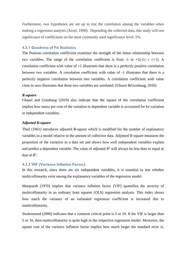
4.3.1 Goodness of Fit Statistics

The Pearson correlation coefficient examines the strength of the linear relationship between

two variables. The range of the correlation coefficient is from -1 to +1(-1≤ r ≤+1). A

correlation coefficient with value of +1 illustrates that there is a perfectly positive correlation

between two variables. A correlation coefficient with value of -1 illustrates that there is a

perfectly negative correlation between two variables. A correlation coefficient with value

close to zero illustrates that these two variables are unrelated. (Ghauri &Gronhaug, 2010)

R-square

Ghauri and Gronhaug (2010) also indicate that the square of the correlation coefficient

implies how many per cent of the variation in dependent variable is accounted for by variation

in independent variables.

Adjusted R-square

Theil (1961) introduces adjusted R-square which is modified for the number of explanatory

variables in a model relative to the amount of collective data. Adjusted R-square measures the

proportion of the variation in a data set and shows how well independent variables explain

and predict a dependent variable. The value of adjusted R2 will always be less than or equal to

that of R2.

4.3.2 VIF (Variance Inflation Factor)

In this research, since there are six independent variables, it is essential to test whether

multicollinearity exist among the explanatory variables of the regression model.

Marquardt (1970) implies that variance inflation factor (VIF) quantifies the severity of

multicollinearity in an ordinary least squares (OLS) regression analysis. This index shows

how much the variance of an estimated regression coefficient is increased due to

multicollinearity.

Studenmund (2006) indicates that a common critical point is 5 or 10. If the VIF is larger than

5 or 10, then multicollinearity is quite high in the respective regression model. Moreover, the

square root of the variance inflation factor implies how much larger the standard error is,

19

compared with what it would be if variables uncorrelated with the other independent variables

in the regression model.

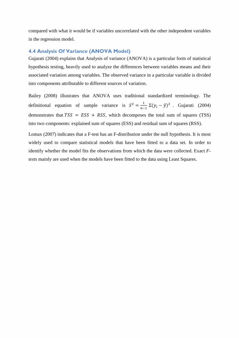
4.4 Analysis Of Variance (ANOVA Model)

Gujarati (2004) explains that Analysis of variance (ANOVA) is a particular form of statistical

hypothesis testing, heavily used to analyze the differences between variables means and their

associated variation among variables. The observed variance in a particular variable is divided

into components attributable to different sources of variation.

Bailey (2008) illustrates that ANOVA uses traditional standardized terminology. The

definitional equation of sample variance is 𝑆2 =1

𝑛−1 Σ(𝑦𝑖 − �̅�)2 . Gujarati (2004)

demonstrates that 𝑇𝑆𝑆 = 𝐸𝑆𝑆 + 𝑅𝑆𝑆, which decomposes the total sum of squares (TSS)

into two components: explained sum of squares (ESS) and residual sum of squares (RSS).

Lomax (2007) indicates that a F-test has an F-distribution under the null hypothesis. It is most

widely used to compare statistical models that have been fitted to a data set. In order to

identify whether the model fits the observations from which the data were collected. Exact F-

tests mainly are used when the models have been fitted to the data using Least Squares.

20

5. Data and Variables

The objective of this thesis is to empirically investigate what is the relationship between

capital structure and corporate performance of 54 listed Swedish firms under the recent

financial crisis during the period 2006 - 2010. Therefore, variables have been divided into

three groups, which are dependent, independent and dummy variables. Based on the previous

empirical literature, authors decided that measurement of capital structure is the dependent

variable and the measurements of firm performance are independent variables. Year dummy

variables will be included in order to illustrate the trend of the relationship in the certain

period.

5.1 Dependent Variable

There is a wide rage of suggestions on relationship between capital structure and company

performance. In this paper a measure of capital structure will be based on leverage. When

studying the annual financial statement in a firm, short-term debt and long –term debt can

easily be found. Liabilities can be divided into short-term debt and long-term debt. Short-term

debt is referred to as current liabilities and long-term debt as long-term liabilities (Adkins,

2011).

Short-term debt is comprised of any debt owned by a business that is due within 12 months. It

is usually made up of short-term bank loans taken out by a corporation (investorwords.com).

Accounts payable, accrued payroll and accrued payroll taxes are examples of short-term debt

(Adkins, 2011).

Long-term debt is any loan within a maturity of more than 12 months. Different kinds of

bonds usually are included in long-term debt; the most common type of long-term debt is a

mortgage’s principal balance. Furthermore, a company often borrows a long-term loan to

make an investment (Berk & DeMarzo, 2007).

Long-term debt creates an interest payment and allows money pay back with interest, which

provide more capital for firms to investment. As the authors mentioned above, mortgage is a

common type of long-term debt, it is usually used to finance purchase of real estates such as

factories, office buildings, or other pieces of real estates. This kind of long-term debt plays a

helpful role in purchasing additional capital assets and making the firm more profitable. In

other word, the corporation prefers to use long-term debt to purchase additional assets or

cover up the firm’s operation expense (Csiszar, 2010).

21

Hence the authors in this paper choose long-term debt ratio as dependent variable. Leverage

ratio created by debt is relation to assets and is used to describe several measures of financial

leverage of a firm.

5.2 Independent Variables

In previous empirical literatures, a number of researchers addressed the measurements of firm

performance. In order to deeply investigate the relationship between capital structure and

corporate performance, five explanatory variables have been considered as the determinants

of financial performance: Profitability, Uniqueness or Growth, Asset composition, Cash

flow/operating revenue and Net Asset turnover.

5.2.1 Profitability

The profitability ratios are commonly used to assess a business's ability to generate earnings

as compared to its expenses and other relevant costs incurred during a specific period of time.

Hansen and Wernerfelt (1989) indicate that profitability ratios are crucial to determine the

firm performance. The most widely used ratios are Return On Asset (ROA) and Gross Margin.

Return On Asset:

Casteuble (1997) suggests that ROA reflects a firm’s financial performance in terms of using

assets to create income. It shows the percentage of profit that a corporation earns in relation to

its overall resources. A firm with higher ROA indicated the better ability of translating assets

into profits. Therefore, it is also called a profitability ratio.

Gross Margin:

Farris, et al (2010) explain that gross margin represents the percent of total sales revenue that

the company retains after considering the direct costs associated with producing the goods and

services sold by a company. The higher gross margin means more earnings the company

retains on each dollar of revenue to service its other costs and obligations.

5.2.2 Uniqueness or Growth

Glaude et al (2009) indicate that Research and Development(R&D) expenditure in European

Union (EU) companies promotes the production of technology and creating innovative ideas.

In certain sectors, R&D investments are essential for the development of production

techniques and the generation of new products. While generally leading to the increased

comparative advantage of the sector in which it is accomplished, R&D expenditure provides

companies with the competence of gaining new and greater market shares. (Eurostat, 2009)

22

In fact, Sweden is an innovation leader on its own merits. The country invests heavily in

research, encourages critical thinking from an early age and is open to international influences:

Ranking No.3 by R&D Expenditure (% of GDP) among the 37 countries. (OECD Factbook

2011–2012).

In this thesis, in order to investigate the Swedish corporate performance deeply, “R&D

Expenditure” has been regarded as the second key measurement of the corporate performance.

Since the other variables are calculated as the percentage, the R&D Expenditure will be

calculated as the percentage of operating revenue.

5.2.3 Cash flow/operating revenue:

According to the International Financial Reporting Standards, operating cash flow defined

that cash generated by a firm’s operation after taxation and interest paid deducted. Operating

cash flow in financial accounting refers to a firm generate amount of cash from the normal

business operation, but the long–term investment cost on capital or investment cost on

securities are not contained in operating cash flow (Ross et al, 2007). The significance of

operation cash flow is that it shows whether a corporation is able to generate sufficient

positive cash flow to maintain its operations, or whether it may require external financing.

Loth (2009) states that cash flow/operating revenue ratio compares the opreation of a firm to

its revenue and gives investors an idea of whether a firm is able to turn sales into cash.

5.2.4 Net Asset turnover

Asset turnover measure a company's use of its assets efficiency in generating sale revenue to

the company (Zane, Kane & Marcus, 2004). It considers the relationship between revenues

and the total assets employed in a business. Asset turnover ratio is a good way for a firm to

generate sales through making its assets work hard. It is calculated by dividing net sales

revenue by average total assets. Asset turnover is negatively related to the gross margin.Firm

with high asset turnover means firm’s profit margins is low, while low asset turnover ratio

represents a high profit margin in a company.

5.3 Dummy Variables

Draper and Smith (1998) point out that, in regression analysis, a dummy variable is one that

takes the value 0 or 1 to indicate the absence or presence of some categorical effect that may

be expected to affect the consequence. A dummy independent variable, which for some

observations has a value of 0, will cause that variable's coefficient to have no influence on the

dependent variable, while when the dummy takes on a value 1 its coefficient intends to

modify the intercept.

23

Since the objective of this thesis is to investigate how the recent financial crisis affects the

relationship between capital structure and corporation performance in 54 listed Swedish

companies. The data is collected from 2006 to 2011. The authors run two regression models

to compare the difference in the coefficients of each variable between the models.

5.3.1 Model 1

In this model, there are five dummy variables, which indicate the different relationship in the

same regression model in different years- Dummy variable 2006, Dummy variable 2007,

Dummy variable 2009, Dummy variable 2010, Dummy variable 2011. Here, year 2008 is

regarded as a basic year since it is the year when recent financial crisis started. They will be

recorded as following:

D2006= 1 if the data collected is in 2006

D2006 = 0 otherwise (any year other than 2006)

D2007= 1 if the data collected is in 2007

D2007 = 0 otherwise (any year other than 2007)

D2009= 1 if the data collected is in 2009

D2009 = 0 otherwise (any year other than 2009)

D2010= 1 if the data collected is in 2010

D2010 = 0 otherwise (any year other than 2010)

D2011= 1 if the data collected is in 2011

D2011 = 0 otherwise (any year other than 2011)

This means that 2008 is reference year.

5.3.2 Model 2

In this model, there is only one dummy variable, which indicates the different relationship in

the same regression model between the pre-financial crisis and post-financial crisis.

DYear = 1 if the data collected is in 2009, 2010, 2011 (Post-Financial Crsis)

DYear = 0 if the data collected is in 2006, 2007, 2008 (Pre-Financial Crisis)

24

6 Empirical Result and Data Analysis

6.1 Descriptive Statistics

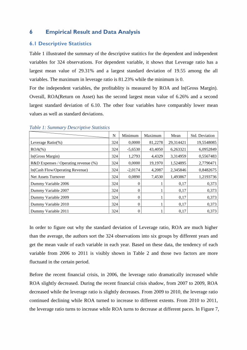
Table 1 illustrated the summary of the descriptive statitics for the dependent and independent

variables for 324 observations. For dependent variable, it shows that Leverage ratio has a

largest mean value of 29.31% and a largest standard deviation of 19.55 among the all

variables. The maximum in leverage ratio is 81.23% while the minimum is 0.

For the independent variables, the profitablity is measured by ROA and ln(Gross Margin).

Overall, ROA(Return on Asset) has the second largest mean value of 6.26% and a second

largest standard deviation of 6.10. The other four variables have comparably lower mean

values as well as standard deviations.

Table 1: Summary Descriptive Statistics

N Minimum Maximum Mean Std. Deviation

Leverage Ratio(%) 324 0,0000 81,2278 29,314421 19,5548085

ROA(%) 324 -5,6530 43,4050 6,263321 6,0952849

ln(Gross Margin) 324 1,2793 4,4329 3,314959 0,5567483

R&D Expenses / Operating revenue (%) 324 0,0000 19,1970 1,524895 2,7790471

ln(Cash Flow/Operating Revenue) 324 -2,0174 4,2087 2,345846 0,8482675

Net Assets Turnover 324 0,0890 7,4530 1,493867 1,2193736

Dummy Variable 2006 324 0 1 0,17 0,373

Dummy Variable 2007 324 0 1 0,17 0,373

Dummy Variable 2009 324 0 1 0,17 0,373

Dummy Variable 2010 324 0 1 0,17 0,373

Dummy Variable 2011 324 0 1 0,17 0,373

In order to figure out why the standard deviation of Leverage ratio, ROA are much higher

than the average, the authors sort the 324 observations into six groups by different years and

get the mean vaule of each variable in each year. Based on these data, the tendency of each

variable from 2006 to 2011 is visibly shown in Table 2 and those two factors are more

fluctuatd in the certain period.

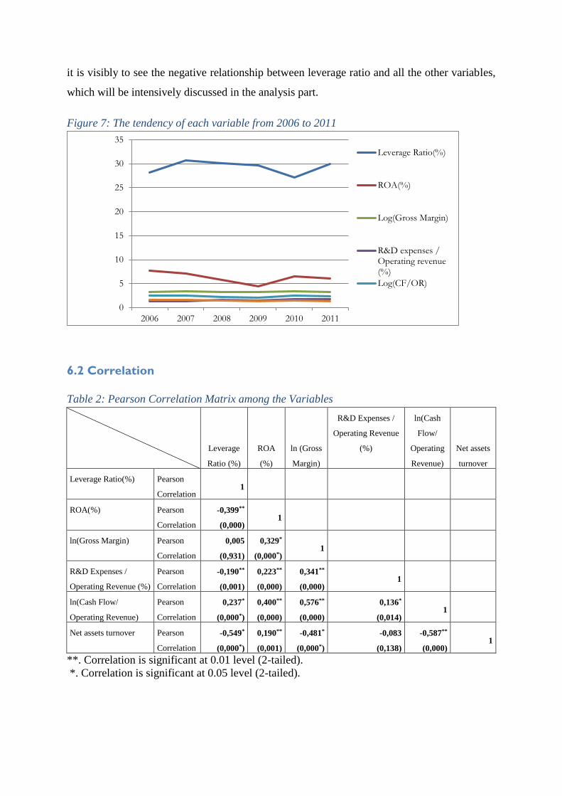
Before the recent financial crisis, in 2006, the leverage ratio dramatically increased while

ROA slightly decreased. During the recent financial crisis shadow, from 2007 to 2009, ROA

decreased while the leverage ratio is slightly decreases. From 2009 to 2010, the leverage ratio

continued declining while ROA turned to increase to different extents. From 2010 to 2011,

the leverage ratio turns to increase while ROA turns to decrease at different paces. In Figure 7,

25

it is visibly to see the negative relationship between leverage ratio and all the other variables,

which will be intensively discussed in the analysis part.

Figure 7: The tendency of each variable from 2006 to 2011

6.2 Correlation

Table 2: Pearson Correlation Matrix among the Variables

Leverage

Ratio (%)

ROA

(%)

ln (Gross

Margin)

R&D Expenses /

Operating Revenue

(%)

ln(Cash

Flow/

Operating

Revenue)

Net assets

turnover

Leverage Ratio(%) Pearson

Correlation 1

ROA(%) Pearson

Correlation

-0,399**

(0,000) 1

ln(Gross Margin) Pearson

Correlation

0,005

(0,931)

0,329*

(0,000*) 1

R&D Expenses /

Operating Revenue (%)

Pearson

Correlation

-0,190**

(0,001)

0,223**

(0,000)

0,341**

(0,000) 1

ln(Cash Flow/

Operating Revenue)

Pearson

Correlation

0,237*

(0,000*)

0,400**

(0,000)

0,576**

(0,000)

0,136*

(0,014) 1

Net assets turnover Pearson

Correlation

-0,549*

(0,000*)

0,190**

(0,001)

-0,481*

(0,000*)

-0,083

(0,138)

-0,587**

(0,000) 1

**. Correlation is significant at 0.01 level (2-tailed).

*. Correlation is significant at 0.05 level (2-tailed).

0

5

10

15

20

25

30

35

2006 2007 2008 2009 2010 2011

Leverage Ratio(%)

ROA(%)

Log(Gross Margin)

R&D expenses /Operating revenue(%)

Log(CF/OR)

26

The authors use Pearson correlation analysis to estimate the relationship among the interval-

level variables. When p-value smaller than 0.05, it illustrates that the correlation between two

variables is significantly different from 0. From table 3, the result shows that the correlation

between leverage ratio and ROA is significant (p-value is 0.000<0.05). Thus, ROA, R&D

expenses, Ln (cash flow/ operating revenue), Net asset turnover is significantly related to

leverage ratio. (corr=-0.399, p-value=0.000; corr=-0.190, p-value=0.001; corr=0.237, p-

value=0.000; corr=-0.549, p-value=0.000).

In addition, the value of the correlation between leverage ratio and ROA, R&D expenses, Net

asset turnover are negative and significant. On the other hand, Ln (Gross Margin) is not

related to the leverage ratio (corr=0.005, p-value=0.931).

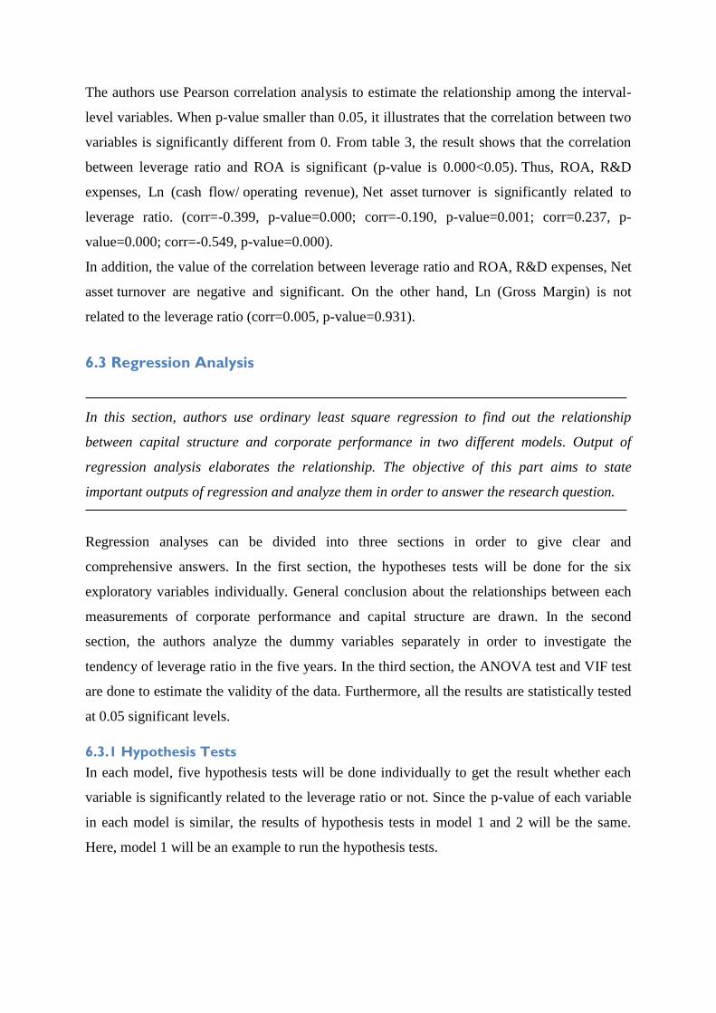
6.3 Regression Analysis

In this section, authors use ordinary least square regression to find out the relationship

between capital structure and corporate performance in two different models. Output of

regression analysis elaborates the relationship. The objective of this part aims to state

important outputs of regression and analyze them in order to answer the research question.

Regression analyses can be divided into three sections in order to give clear and

comprehensive answers. In the first section, the hypotheses tests will be done for the six

exploratory variables individually. General conclusion about the relationships between each

measurements of corporate performance and capital structure are drawn. In the second

section, the authors analyze the dummy variables separately in order to investigate the

tendency of leverage ratio in the five years. In the third section, the ANOVA test and VIF test

are done to estimate the validity of the data. Furthermore, all the results are statistically tested

at 0.05 significant levels.

6.3.1 Hypothesis Tests

In each model, five hypothesis tests will be done individually to get the result whether each

variable is significantly related to the leverage ratio or not. Since the p-value of each variable

in each model is similar, the results of hypothesis tests in model 1 and 2 will be the same.

Here, model 1 will be an example to run the hypothesis tests.

27

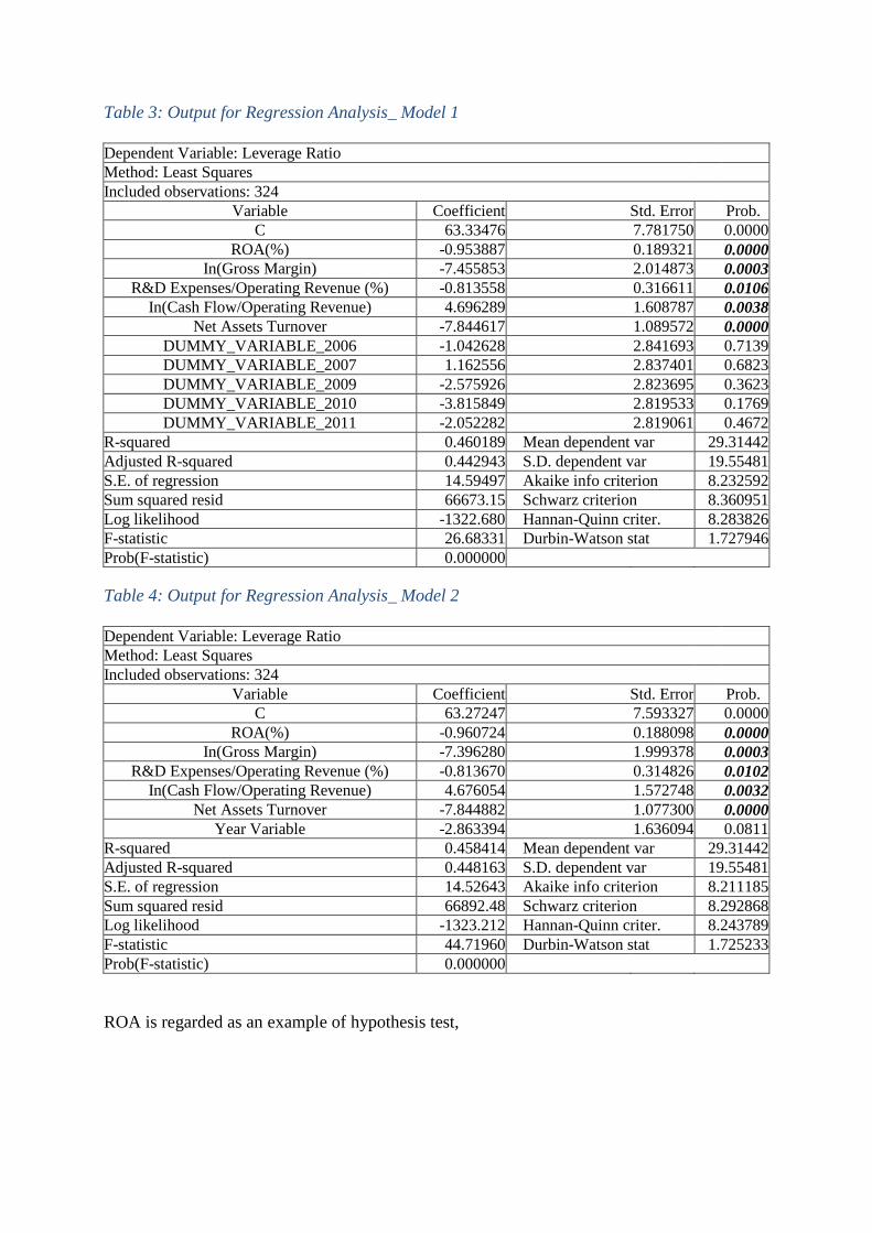
Table 3: Output for Regression Analysis_ Model 1

Dependent Variable: Leverage Ratio

Method: Least Squares

Included observations: 324

Variable Coefficient Std. Error Prob.

C 63.33476 7.781750 0.0000

ROA(%) -0.953887 0.189321 0.0000

In(Gross Margin) -7.455853 2.014873 0.0003

R&D Expenses/Operating Revenue (%) -0.813558 0.316611 0.0106

In(Cash Flow/Operating Revenue) 4.696289 1.608787 0.0038

Net Assets Turnover -7.844617 1.089572 0.0000

DUMMY_VARIABLE_2006 -1.042628 2.841693 0.7139

DUMMY_VARIABLE_2007 1.162556 2.837401 0.6823

DUMMY_VARIABLE_2009 -2.575926 2.823695 0.3623

DUMMY_VARIABLE_2010 -3.815849 2.819533 0.1769

DUMMY_VARIABLE_2011 -2.052282 2.819061 0.4672

R-squared 0.460189 Mean dependent var 29.31442

Adjusted R-squared 0.442943 S.D. dependent var 19.55481

S.E. of regression 14.59497 Akaike info criterion 8.232592

Sum squared resid 66673.15 Schwarz criterion 8.360951

Log likelihood -1322.680 Hannan-Quinn criter. 8.283826

F-statistic 26.68331 Durbin-Watson stat 1.727946

Prob(F-statistic) 0.000000

Table 4: Output for Regression Analysis_ Model 2

Dependent Variable: Leverage Ratio

Method: Least Squares

Included observations: 324

Variable Coefficient Std. Error Prob.

C 63.27247 7.593327 0.0000

ROA(%) -0.960724 0.188098 0.0000

In(Gross Margin) -7.396280 1.999378 0.0003

R&D Expenses/Operating Revenue (%) -0.813670 0.314826 0.0102

In(Cash Flow/Operating Revenue) 4.676054 1.572748 0.0032

Net Assets Turnover -7.844882 1.077300 0.0000

Year Variable -2.863394 1.636094 0.0811

R-squared 0.458414 Mean dependent var 29.31442

Adjusted R-squared 0.448163 S.D. dependent var 19.55481

S.E. of regression 14.52643 Akaike info criterion 8.211185

Sum squared resid 66892.48 Schwarz criterion 8.292868

Log likelihood -1323.212 Hannan-Quinn criter. 8.243789

F-statistic 44.71960 Durbin-Watson stat 1.725233

Prob(F-statistic) 0.000000

ROA is regarded as an example of hypothesis test,

28

H0: β1 =0 (there is no significantly different from zero) against H1: β1 ≠ 0 (there is

significantly different from zero) at 5% significance level, with d.f. (Degree of freedom)

312(=323-11)

The p-value is 0.0000 < significant level = 0.05. Therefore, H0 is rejected, which interprets

there is significant relationship between ROA and Leverage Ratio. In Table 3, it is shown that

the coefficient of ROA is -0.953887, which interprets ROA is negative significantly

correlated to the Leverage Ratio: when ROA increases by one unit, Leverage ratio will

decrease by 0.95 units.

The rest of the hypothesis tests are done in the same way. In the Table 3 and 4, it is shown

that the P-value of ln(Gross Margin), R&D expenses/Operating Revenue, In (Cash

Flow/Operating Revenue) and Net asset turnover are less than the significant level (= 0.05).

These results of hypothesis tests interpret that ROA, ln(Gross Margin), R&D

expenses/Operating Revenue and Net asset turnover have significant relationships with

leverage ratio. Moreover, in Table 3 and 4, it states that the coefficients of ROA, ln (Gross

Margin), R&D expenses/Operating Revenue and Net asset turnover are with minus sign and

only the coefficient of In (Cash Flow/Operating Revenue) is with plus sign. These signs state

that the ROA, ln (Gross Margin), R&D expenses/Operating Revenue and Net asset turnover

are negative significantly correlated to the Leverage Ratio while In (Cash Flow/Operating

Revenue) is positive significantly correlated to the Leverage Ratio.

Overall, the relationship between capital structure and corporation performance in the listed

Swedish companies under the financial crisis is statistical significant and negative.

6.3.4 Interpretations of Dummy Variables

Model 1

The initial regression model in this thesis is estimated as follows

Leverage ratio = β0 + β1 ROA + β2 ln (Gross Margin) +β3 (R&D expenses/ Operating

Revenue) + β4 ln (Cash Flow/ Operating Revenue) + β5 Net Asset Turnover

+ β6 D2006 +β7 D2007 + β8 D2009 + β9 D2010 + β10 D2011 + 𝜀

After the regression model has been done, the formula for the predicted variable can be

written as following:

Leverage ratio = 63.33476 - 0.953887 ROA - 7.455853 ln(Gross Margin) - 0.813558 (R&D

expenses/ Operating Revenue) + 4.696289 ln(Cash Flow/ Operating Revenue) - 7.844617 Net

29

Asset Turnover - 1.042628 D2006 + 1.162556 D2007 - 2.575926 D2009 - 3.815849 D2010 -

2.052282 D2011

After the hypotheses tests have been done for the five exploratory variables individually, the

general conclusion about the relationships between each measurements of corporate

performance and capital structure has been drawn. The other objective of this thesis is to find

how the recent financial crisis affects the relationship between capital structure

and corporate performance in listed Swedish companies. In order to illustrate this relationship

more deeply, the dummy variables should be taken into consideration individually.

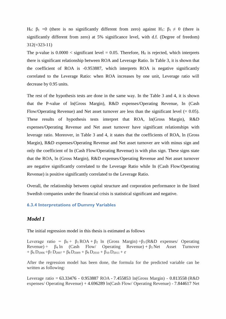
Figure 8 Leverage Ratio Tendencies

In the Figure 8, it is shown that the leverage ratio dramatically goes up from 2006 to 2007,

which is from - 1.04 to + 1.16. Then it decreases sharply from 2007 to 2009, which is from

+ 1.16 to -2.58. Continuously, it slightly goes down from 2009 to 2010, which is from -2.58

to -3.82. Howver, the tendency turns to go up after 2010. There is a dramatically increase

from 2010 to 2011, which is from -3.82 to - 2.05. Since the peak of the leverage is in 2007

among these six years and the recent financial crisis started in 2008. Empirically, this table

illustreted that the recent global Financial Crisis leads the leverage ratio increase among 54

listed Swedish companies at the beginning, and further stimulates the leverage ratio decline to

the lower level after the financial crisis starts in 2008, but in the end, it goes up to the normal

leverage ratio, which is nearly the same level as 2006, before the current financial crisis.

Model 2

The initial regression model in this thesis is drawn as following:

Leverage ratio = β0 + β1 ROA + β2 ln (Gross Margin) +β3 (R&D expenses/ Operating Revenue)

+ β4 ln (Cash Flow/ Operating Revenue) + β5 Net Asset Turnover + β6 DYear+ 𝜀

After the regression model has been estimated, the formula can be written as following:

-1,04

1,16

-2,58

-3,82

-2,05

-5

-4

-3

-2

-1

0

1

2

2006 2007 2009 2010 2011

30

Leverage ratio = 63.27247 - 0.960724 ROA - 7.396280 ln (Gross Margin) - 0.813670 (R&D

expenses/ Operating Revenue) + 4.676054 ln (Cash Flow/ Operating Revenue) - 7.844882Net

Asset Turnover - 2.863394 DYear

Regardless of other exploratory variables, the dummy variables invisibly affect the intercept

of this regression model. In the other word, the leverage ratio is fluctuated by year factors.

Pre-Financial Crisis:

Leverage ratio = 63.27247 - 0.960724 ROA - 7.396280 ln (Gross Margin) - 0.813670 (R&D

expenses/ Operating Revenue) + 4.676054 ln (Cash Flow/ Operating Revenue) - 7.844882Net

Asset Turnover

Post-Financial Crisis:

Leverage ratio = 63.27247 - 0.960724 ROA - 7.396280 ln (Gross Margin) - 0.813670 (R&D

expenses/ Operating Revenue) + 4.676054 ln (Cash Flow/ Operating Revenue) - 7.844882Net

Asset Turnover - 2.863394

Based on these two regression equations, thet are shown that the leverage ratio in Pre-

Financial Crisis (2006, 2007, 2008) is higher than that in Post- Financial Crisis (2009, 2010,

2011). Since p-value of this year yummy is 0.08, which is higher than 0.05 significant level,

it is not significant.

6.3.2 Goodness of Fit Statistics

6.3.2.1 Adjusted R-Square

Adjusted R square is useful only if R square is calculated based on a sample, not the entire

population (Cameron& Windmeir, 1996). In addition, adjusted R square is related to the

numbers of variables and observations and the adjusted R2 would be better index to measure

the goodness of fit statistics in the regression model with more than one independent

variables. There is more than one independent variable in this case, therefore the authors

choose adjusted R2 instead of R2. The values of Adjusted R-square in two Models are

0.442943 and 0.448163, which means 44 per cent of the total variance in leverage ratio has

been explained. In other words, the correlation could be defined as comparably weak but

explains a significant part of the variance in the analysis.

6.3.2.2 Variance Inflation factor (VIF)

Variance inflation factor (VIF) quantifies the severity of multicollinearity and interprets how

much the variance of an estimated regression coefficient is increased due to multicollinearity.

Model 1

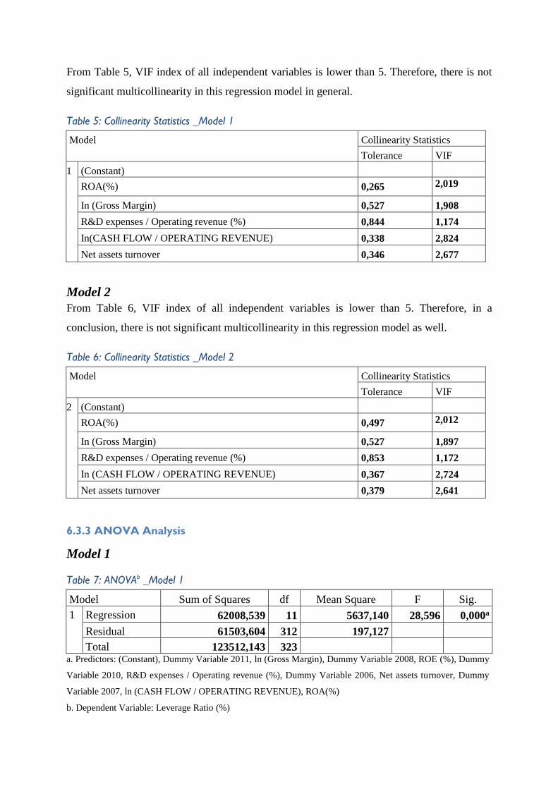
31

From Table 5, VIF index of all independent variables is lower than 5. Therefore, there is not

significant multicollinearity in this regression model in general.

Table 5: Collinearity Statistics _Model 1

Model Collinearity Statistics

Tolerance VIF

1 (Constant)

ROA(%) 0,265 2,019

In (Gross Margin) 0,527 1,908

R&D expenses / Operating revenue (%) 0,844 1,174

In(CASH FLOW / OPERATING REVENUE) 0,338 2,824

Net assets turnover 0,346 2,677

Model 2

From Table 6, VIF index of all independent variables is lower than 5. Therefore, in a

conclusion, there is not significant multicollinearity in this regression model as well.

Table 6: Collinearity Statistics _Model 2

Model Collinearity Statistics

Tolerance VIF

2 (Constant)

ROA(%) 0,497 2,012

In (Gross Margin) 0,527 1,897

R&D expenses / Operating revenue (%) 0,853 1,172

In (CASH FLOW / OPERATING REVENUE) 0,367 2,724

Net assets turnover 0,379 2,641

6.3.3 ANOVA Analysis

Model 1

Table 7: ANOVAb _Model 1

Model Sum of Squares df Mean Square F Sig.

1 Regression 62008,539 11 5637,140 28,596 0,000a

Residual 61503,604 312 197,127

Total 123512,143 323

a. Predictors: (Constant), Dummy Variable 2011, ln (Gross Margin), Dummy Variable 2008, ROE (%), Dummy

Variable 2010, R&D expenses / Operating revenue (%), Dummy Variable 2006, Net assets turnover, Dummy

Variable 2007, ln (CASH FLOW / OPERATING REVENUE), ROA(%)

b. Dependent Variable: Leverage Ratio (%)

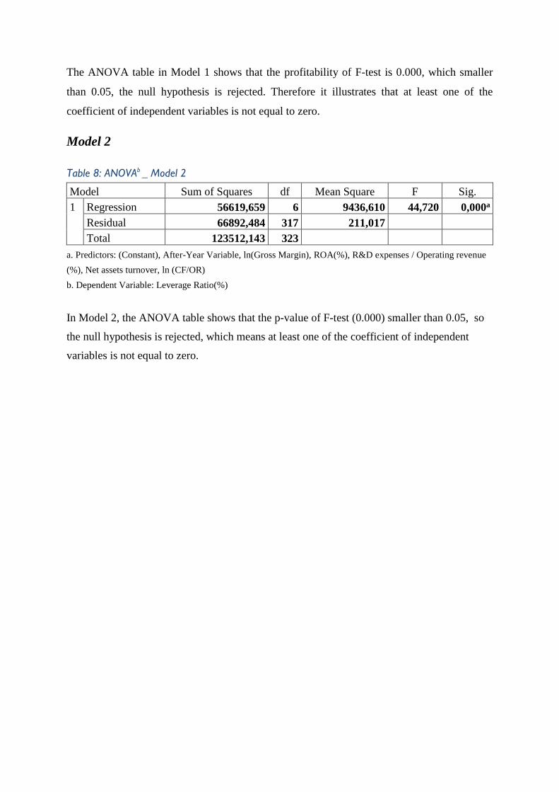
32

The ANOVA table in Model 1 shows that the profitability of F-test is 0.000, which smaller

than 0.05, the null hypothesis is rejected. Therefore it illustrates that at least one of the

coefficient of independent variables is not equal to zero.

Model 2

Table 8: ANOVAb _ Model 2

Model Sum of Squares df Mean Square F Sig.

1 Regression 56619,659 6 9436,610 44,720 0,000a

Residual 66892,484 317 211,017

Total 123512,143 323

a. Predictors: (Constant), After-Year Variable, ln(Gross Margin), ROA(%), R&D expenses / Operating revenue

(%), Net assets turnover, ln (CF/OR)

b. Dependent Variable: Leverage Ratio(%)

In Model 2, the ANOVA table shows that the p-value of F-test (0.000) smaller than 0.05, so

the null hypothesis is rejected, which means at least one of the coefficient of independent

variables is not equal to zero.

33

7 Concluding Remarks

Based on the theoretical framework and empirical findings from the data and the regression

analysis, the research questions and sub-questions could be solved. In the end,

recommendations will also be suggested to researchers that desire to further study in this

area.

7.1 Answer to Research Questions

What is the relationship between capital structure and corporation

performance in listed 54 Swedish companies under the recent financial

crisis?

In the previous literature review, there are a large amount of researches that draw an empirical

conclusion of the relationship between capital structure and corporate performance. Based on

this empirical findings and analysis, there is a negative significantly relationship between

capital structure and corporate performance for 54 Swedish listed companies in general.

However, the authors find a couple of different relationships when analyzing our findings in

detail. In this regression model 1, there is one dependent variable as the measurement of

capital structure, five exploratory independent variables as measurements of corporate

performance and five dummy variables as time factors. In model 2, five exploratory

independent variables as measurements of corporate performance, one dependent variable as

the measurement of capital structure, there is only one dummy variable in regression model.

Sub-research question 1: What are the determinants of the corporation performance?

In this study, five independent variables based measurement of financial performance are

used, which are profitability, Uniqueness or Growth, Asset composition, Cash flow/operating

revenue and Net Asset turnover to determine the firm performance.

The profitability ratios play a significant role in the determinants of firm performance

(Hansen &Wernerfelt, 1989). Return On Asset (ROA) and Gross Margin are the most widely

used profitability ratios. ROA represents the ability of a firm to translate assets into profits, it

shows the percentage of profit that earning of a firm relate to its overall resources. Growth

margin calculated as the revenue minus the cost of good sold, then divided by revenue, which

indicates earnings the company retains on each dollar of revenue to service its other costs and

obligations. R & D expenses are crucial to the development of production techniques and the

generation of new products. It has been regarded as the second key measurement of the

34

corporate performance in this paper. Moreover, cash flow/operating revenue ratio gives

investors an idea of whether a firm is able to turn sales into cash and Net Asset turnover asset

turnover ratio is imagining the business try to make its assets work hard to generate sales.

Both of them also have been considered as the determinants of financial performance.

Sub-research question 2: What is the relationship between each determinant of

corporation performance and capital structure?

In the two models, the coefficient and P-value of each variable is similar. Therefore, the

results indicated that the relationship between each determinant of corporation performance

and capital structure does not significant effect between each other. And we can make the

general conclusion as following:

After hypothesis testing of each exploratory independent variable, it is shown that all five

independent variables have significantly relationships with capital structure – ROA, Gross

Margin, R&D Expenses and Net Assets Turnover have significantly negative relationships

with capital structure while only Cash Flow/Operating Revenue have a significantly positive

relationship with capital structure.

In general, the relationship between capital structure and corporation performance in listed 54

Swedish companies under the recent financial crisis is significantly negative.

Sub-research question 3: What is the debt ratio tendency before and after the financial

crisis among 54 listed Swedish companies?

Since the results of two regression models reveals that the relationship between capital

structure and corporation performance in listed 54 Swedish companies under the recent

financial crisis is generally similar. The difference is measured by the coefficients of dummy

variables, which indicate the difference in intercepts. In Model 1 (Figure 7), it could be

concluded that the debt ratio increases dramatically before the recent financial crisis (from

2006 to 2007) and then sharply declines afterwards (from 2007 to 2010), but in the end (in

2011) is back to the previous level of leverage ratio as before the financial crisis. In Model 2

(Table 5), the coefficient of the Year Dummy Variable is -2.863394, which indicates the

leverage ratio in pre-financial crisis (from 2006 to 2008) is generally higher than that in post-

financial crisis (from 2009 to 2011). This conclusion also coincides with Figure 7, which

shows that leverage ratio from 2006 to 2008 is above zero while leverage ratio from 2009 to

2011 is below zero.

35

Empirically, an increase in leverage ratio can lead companies get more benefit form debt,

however when the level reaches to peak or certain level, it may cause the recent financial

crisis to some extents since companies cannot pay off the larger amount of debt and they

have to apply for the bankruptcy. Here, managers of Swedish companies have chosen higher

leverage ratios from 2006 to 2007, which is the peak in leverage ratio over the observation

period. At this point, the recent financial crisis has potentially started. During the recent

financial crisis, the managers of Swedish companies adjusted to this global financial crisis in

the coming year. Therefore, the leverage ratio of general Swedish companies declined from

2008 to 2010. When the leverage ratio reaches the bottom level in 2010, it turned to go up to

the previous leverage ratio in year 2011, when the same leverage ratio can be seen as before

the financial crisis started.

To conclude, in general, there is a significantly negative relationship between capital

structure and corporation performance in listed 54 Swedish companies under the recent

financial crisis. Based on the trade-off theory, if debt ratio is higher than the optimal capital

structure, firm of value will decline when leverage ratio increase. Therefore, the leverage

ratio is higher than the optimal leverage ratio during the financial crisis. The general higher

leverage ratio leads the relationship to negative.

7.2 Future Research Recommendation

After the reflection on the whole research, the authors of this thesis find there are several

weaknesses of our analysis in the different sectors. And it would be helpful for future

researchers to avoid these weaknesses in this certain field.

The data of this research is 54 companies, which is selected from the TOP 250 largest

Swedish companies. Smith and Stulz (1985) stated that capital structure has

pronounced industry patterns, and these are the identical around the world. It could be

better for the future researchers to lower this weakness by sorting the overall data into

different industries. Then different regression models would be run by the certain

industries.

Different independent variables such as Return on investment (ROI), EBIT/ Sales ratio

may also be included in the further research to test whether the different result occurs.

In addition, a further selection could for instance add more dependent variables such

as short-term debt ratio and long-term ratio so that more models are created to analyze

the capital structure-firm performance relationship.

36

8 Appendix 1_ Names of Listed 54 Swedish Company

ABB NORDEN HOLDING AB

AKTIEBOLAGET ELECTROLUX

AKTIEBOLAGET SKF

AKTIEBOLAGET VOLVO

ALBERT BONNIER AB

ALFA LAVAL AB

ASSA ABLOY AB

ATLAS COPCO AKTIEBOLAG

ATTENDO AB (PUBL)

AUTOLIV AKTIEBOLAG

AXEL JOHNSON AKTIEBOLAG

AXEL JOHNSON HOLDING

AKTIEBOLAG

BONNIER AB

BRANÄS GRUPPEN AB

ERICSSON AB

ESCO MARGINALEN AB

GETINGE AB

GRÖNKLITTSGRUPPEN AB (PUBL)

H & M HENNES & MAURITZ AB

HEXAGON AKTIEBOLAG

HUSQVARNA AKTIEBOLAG

ICA AB

INVESTOR AKTIEBOLAG

JSM GRUPPEN AB

KALMAR KOMMUNBOLAG AB

LANDSTINGSHUSET I STOCKHOLM

AKTIEBOL

LOOMIS AB

NCC AKTIEBOLAG

NORDSTJERNAN AKTIEBOLAG

NÅIDEN AB

PEAB AB

POSTEN MEDDELANDE AB

POSTNORD AB

RATOS AB

SAAB AKTIEBOLAG

SAMHALL AKTIEBOLAG

SANDVIK AKTIEBOLAG

SAPA AB

SAS AB

SCANIA AKTIEBOLAG

SCANIA CV AKTIEBOLAG

SECURITAS AB

SKANSKA AB

SONY MOBILE COMMUNICATIONS

AB

STAXERED INVEST AB

STENA AKTIEBOLAG

SVENSKA CELLULOSA

AKTIEBOLAGET SCA

TELEFONAKTIEBOLAGET L M

ERICSSON

TELIASONERA AKTIEBOLAG

TOYOTA INDUSTRIES EUROPE AB

TRELLEBORG AB

VATTENFALL AKTIEBOLAG

VOLVO PERSONVAGNAR

AKTIEBOLAG

YGEIA TOPHOLDING AB

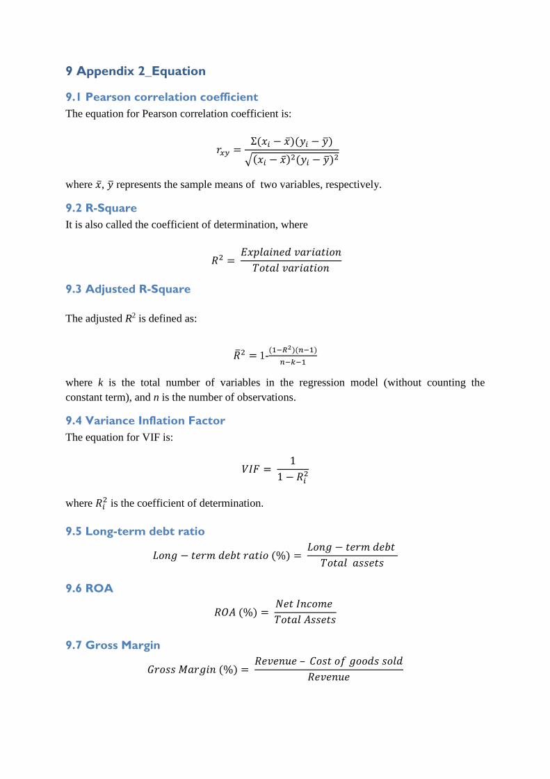
2

9 Appendix 2_Equation

9.1 Pearson correlation coefficient

The equation for Pearson correlation coefficient is:

𝑟𝑥𝑦 =Σ(𝑥𝑖 − �̅�)(𝑦𝑖 − �̅�)

√(𝑥𝑖 − �̅�)2(𝑦𝑖 − �̅�)2

where �̅�, �̅� represents the sample means of two variables, respectively.

9.2 R-Square

It is also called the coefficient of determination, where

𝑅2 = 𝐸𝑥𝑝𝑙𝑎𝑖𝑛𝑒𝑑 𝑣𝑎𝑟𝑖𝑎𝑡𝑖𝑜𝑛

𝑇𝑜𝑡𝑎𝑙 𝑣𝑎𝑟𝑖𝑎𝑡𝑖𝑜𝑛

9.3 Adjusted R-Square

The adjusted R2 is defined as:

�̅�2 = 1-(1−𝑅2)(𝑛−1)

𝑛−𝑘−1

where k is the total number of variables in the regression model (without counting the

constant term), and n is the number of observations.

9.4 Variance Inflation Factor

The equation for VIF is:

𝑉𝐼𝐹 = 1

1 − 𝑅𝑖2

where 𝑅𝑖2 is the coefficient of determination.

9.5 Long-term debt ratio

𝐿𝑜𝑛𝑔 − 𝑡𝑒𝑟𝑚 𝑑𝑒𝑏𝑡 𝑟𝑎𝑡𝑖𝑜 (%) = 𝐿𝑜𝑛𝑔 − 𝑡𝑒𝑟𝑚 𝑑𝑒𝑏𝑡

𝑇𝑜𝑡𝑎𝑙 𝑎𝑠𝑠𝑒𝑡𝑠

9.6 ROA

𝑅𝑂𝐴 (%) = 𝑁𝑒𝑡 𝐼𝑛𝑐𝑜𝑚𝑒

𝑇𝑜𝑡𝑎𝑙 𝐴𝑠𝑠𝑒𝑡𝑠

9.7 Gross Margin

𝐺𝑟𝑜𝑠𝑠 𝑀𝑎𝑟𝑔𝑖𝑛 (%) = 𝑅𝑒𝑣𝑒𝑛𝑢𝑒 – 𝐶𝑜𝑠𝑡 𝑜𝑓 𝑔𝑜𝑜𝑑𝑠 𝑠𝑜𝑙𝑑

𝑅𝑒𝑣𝑒𝑛𝑢𝑒

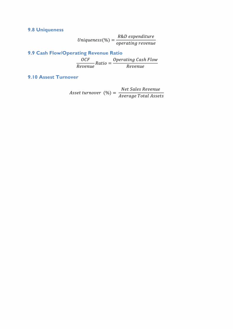
3

9.8 Uniqueness

𝑈𝑛𝑖𝑞𝑢𝑒𝑛𝑒𝑠𝑠(%) =𝑅&𝐷 𝑒𝑥𝑝𝑒𝑛𝑑𝑖𝑡𝑢𝑟𝑒

𝑜𝑝𝑒𝑟𝑎𝑡𝑖𝑛𝑔 𝑟𝑒𝑣𝑒𝑛𝑢𝑒

9.9 Cash Flow/Operating Revenue Ratio

𝑂𝐶𝐹

𝑅𝑒𝑣𝑒𝑛𝑢𝑒𝑅𝑎𝑡𝑖𝑜 =

𝑂𝑝𝑒𝑟𝑎𝑡𝑖𝑛𝑔 𝐶𝑎𝑠ℎ 𝐹𝑙𝑜𝑤

𝑅𝑒𝑣𝑒𝑛𝑢𝑒

9.10 Assest Turnover

𝐴𝑠𝑠𝑒𝑡 𝑡𝑢𝑟𝑛𝑜𝑣𝑒𝑟 (%) = 𝑁𝑒𝑡 𝑆𝑎𝑙𝑒𝑠 𝑅𝑒𝑣𝑒𝑛𝑢𝑒

𝐴𝑣𝑒𝑟𝑎𝑔𝑒 𝑇𝑜𝑡𝑎𝑙 𝐴𝑠𝑠𝑒𝑡𝑠

4

10 References

Actuarial Science Studies (2012). Actuarialsciencestudies.blogspot.se. Retrieved 2012-06-05, from

http://actuarialsciencestudies.blogspot.se/2012/03/trade-off-theory.html

Adkins, W. D. (2011). The determination of long-term credit standing with financial ratios.

Journal of Accounting Research, 44-62.

Akbar, A. J., Javadian, H., & Kootanaee, H. J., (2012). A comparison of performance

measures for finding the best measure of business entity performance. Journal of Finance and

Investment Analysis, 1(4), 27-35.

Altman, E. I. (1984). A further empirical investigation of the bankruptcy cost question.

Journal of Finance, 39 , 1067–1089.

Artis, M. J., & Zhang, W. (1997). International business cycles and the ERM: Is there a

European business cycle. International Journal of Finance and Economics, 2(1), 1–16.

Bailey, R. A. (2008). Design of Comparative Experiments. London: Cambridge University

Press.

Berk, J., & DeMarzo, P. (2007). Corporate Finance. Boston: Addison Wesley.

Baumol, W. J., & Malkiel, B. G. (1968). Earnings retention, new capital and the growth of the

firm. The Review of Economics and Statistics, 52(4), 345-355.

Baxter, N. (1967). Leverage, risk of ruin and the cost of capital. Journal of Finance, 22, 395–

403.

Bistrova, J., Lace, N., & Peleckienė, V. (2011). The influence of capital structure on Baltic

corporate performance. Journal of Business Economics and Management, 12(4), 655-669.

Bradley, M., Jarrell, G., & Kim, E. H. (1984). On the existence of an optimal capital structure:

theory and evidence. The Journal of Finance ,39, 857-878.

Campello, M. (2006). Debt Financing: Does it boost or hurt firm performance in product

markets? Journal of Financial Economics, 82(1), 135-172.

Casteuble, T. (1997). What today’s association executives earn. Association Management,

49(4), 53-61.

Chemmanur, T.,& Fulghieri, P. (1994). Reputation, renegotiation, and the choice between

bank loans and publicly traded debt. Review of Financial Studies, 7(3),475-506.

Ketels. C. (2012). Sweden’s Position In the Global Economy. Sweden:

Entreprenörskapsforum.

Csiszar, J. (2010, March 29). What is financial leverage and how is it provided by long-term

debt? Retrieved 2013-05-16 from http://www.answerbag.com/q_view/1978789

5

Dalene, K., & Stangl, D. K. (2012). Encyclopaedia of statistics in behavioural science.

Journal of the American Statistical Association, 103(482), 881-882.

Delamont, S. (1992). Teachers’ pedagogical systems and grammar teaching: A qualitative

study. TESOL Quarterly, 32(1), 9-38.

Damodaran, A. (2001). Corporate Finance: Theory and Practice. New York: Wiley.

Modigliani, F., & Miller, M. (1958). The cost of capital, corporation finance and the theory of

investment. The American Economic Review, 48(3), 261-97.

De Mooij, R. (2011). Tax biases to debt finance: Assessing the problem. Fiscal Studies, 33(4),

489-512.

DeAngelo, H., & Masulis, R. W. (1980). Optimal capital structure under corporate and

personal taxation. The Journal of Financial Economics, 8, 3-29.

Delamont, S. (1992). Fieldwork in Educational Settings: Methods, Pitfalls and Perspectives.

London: Falmer.

Draper, N. R., & Smith, H. (1998). Applied Regression Analysis. New York: Wiley.

Dziuda, W., & Mondria, J. (2012). Asymmetric information, portfolio managers, and home

bias. Journal of Economic Literature, 51(1), 63-115.

Farris, P. W., Bendle, N. T., Pfeifer, P. E., & Reibstein, D. J. (2010). Marketing metrics: The

definitive guide to measuring marketing performance. New Jersey: Pearson Education

Ferris, S., Jayaraman, N., & Makhija, A. (1997). Direct costs of bankruptcy: evidence from

filings of liquidations and reorganizations by small firm. Advances In Financial Economics, 3,

159-186.

Fosberg, R. H. (2011). Capital structure and the financial crisis. Journal of Finance

Accountancy, 1-11.

Modigliani, F., & Miller, M. H. (1963). Corporate income taxes and the cost of capital: A

correction. The American Economic Review,53(3), 433-443.

Kwansa, F. A., & Cho, M. H. (1995). Bankruptcy cost and capital structure: the significance

of indirect cost. International Journal of Hospitality Management, 14(3), 339-350.

Frank, M. Z., & Goyal, V. K. (2003). Testing the pecking order theory of capital structure.

Journal of Financial Economics, 67, 217–248.

Fruhan, W. E., Jr, W. C. ,& Kester, S. P. (1992). Teacher's Manual for Case Problems in

Finance. IL: Irwin.

Glaude, M. et al (2009). Science, Technology and Innovation in Europe, Eurostat

Pocketbooks, 15-30

6

Ghauri, P., Gronhaug, K., & Kristinslund, I. (2010). Research Methods in Business Studies,

Edinburgh: FT.

Ghosh, A., Cai, F., & Fosberg, R. H. (2007). Capital structure and firm performance. United

States: ANS.

Given, L. M. (2008). The SAGE encyclopedia of qualitative research methods. Los Angeles,

Calif.: Sage Publications.

Gleason, K. C., Mathur, L. K., & Mathur, I. (2000). The interrelationship between cultures,

capital structure, and performance: Evidence from European retailers. Journals of Business

Research, 50,185-91.

Gujarati, D. N.(2004). Basic Econometrics, New York: The McGraw−Hill Companies.

Hamada, R. S. (1969). Portfolio analysis, market equilibrium and corporation finance. The

Journal of Finance, 24(1), 13-31.

Hansen, B. E. (1996). ECONOMETRICS: the likelihood ratio test under nonstandard

conditions: testing the Markov switching model of GNP. Journal of Applied econometrics,

11(2), 195-198.

Hansen, S. G., & Wernerfelt, B. (1989). Determinants of firm performance: The relative

importance of economic and organizational factors. Strategic Management Journal, 10(5),

399-411.

Harris, M., & Raviv, A. (1991). The theory of capital structure. The Journal of Finance,

46(1), 297-355.

Hatfield, G. B., Louis, T. W., & Davidson, W. N. (Fall 1994). The determination of optimal

capital structure: The effect of firm and industry debt ratios on market value. Journal of

Financial And Strategic Decisions, 7(3).

Haugen, R. A., & Senbet, L. W. (1978). The insignificance of bankruptcy costs to the theory

of optimal capital structure. Journal of Finance, 33(2), 383-393.

Hillier, D. J., Ross, S. A., Westerfield, R. W., Jaffe, J. J., & Jordan, B. D. (2010). Corporate

Finance. Maidenhead: McGraw Hill Higher Education.

Hoshi, T., Kashyap, A., & Scharfstein, D. (1990). The role of banks in reducing the costs of

financial distress in Japan. The Journal of Financial Economics, 27(1), 67-88.

Hutchinson, R. W. (1995). The capital structure and investment decisions of the small owner-

managed firm: Some explanatory issues. Small Business Economics, 7, 231.

Investor.com.(2005). Long-term debt. Retrieved 2013-03-24 from

http://www.investorwords.com/2888/long_term_debt.html

Jensen, M. C., & Meckling, W. H. (1976). Theory of the firm: managerial behaviour, agency

costs and ownership structure. Journal of Financial Economics, 3(4), 305-360.

7

Johanson, M. (2009,October 01). The Swedish authorities take a stand IFLR.com. Retrieved

2013-05-16, from http://www.iflr.com/Article/2324193/Sweden-The-Swedish-authorities-

takes-a-stand.html K. F. K. Bank (2013). kfknowledgebank.com. Retrieved 2013-06-02, from

http://kfknowledgebank.kaplan.co.uk/KFKB/Wiki%20Pages/Theories%20of%20Gearing.aspx

Kalemli, S. O., Sorensen, B., & Yesiltas, S. (2011). Leverage across firms, banks, and

countries. Journal of International Economics, 88(2), 284-298.

Ketels, C. (Eds.). (2009). Clusters, Cluster Policy, and Swedish Competitiveness in the Global

Economy. Västerås: The Globalisation Council.

Kraus, A., & Litzenberger, R. H. (1973). A state-Preference model of optimal financial

leverage. Journal of Finance, 28(4),911-922.

Krishnamurthy, A. (2010). How debt markets have malfunctioned in the crisis. Journal of

Economic Perspectives, 24(1), 3-28.

Lafaille, R., & Wildeboer, H. (1995). Validity and reliability of observation and data,

collection in biographical research. Belgium: The International Institute for Advanced Health

Studies.

Lomax, R. G. (2007). Statistical Concepts: A Second Course. Mahwah, NJ: Lawrence

Erlbaum.

Loth, R. (2009). Cash flow indicator patios. Retrieved 2013-05-16 from

http://www.investopedia.com/university/ratios/cash-flow-indicator/ratio1.asp

Marquardt, D.W. (1970). Generalized inverses, ridge regression, biased linear estimation, and

nonlinear estimation, Technometrics, 12(3), 591, 605–607.

Martin, F., & Green, J. (1983). Why do companies pay dividends? The American Economic

Review, 73(1) ,17-30.

McKibbin, W. J., & Stoeckel, A. (2009). The Global Financial Crisis: Causes and

Consequences. Asian Economic Papers, 9(1), 54-86.

Megginson, W. L., & Smart, S. B. (2008). Introduction to Corporate Finance. USA: LEAP

publishinf service.Inc..

Modigliani, F., & Miller, M. H. (1958). The cost of capital, corporation finance and the theory

of investment. The American Economic Review, 48(3), 261-297.

Modigliani, F., & Miller, M. H. (1963). Corporate income taxes and the cost of capital: A

correction. American Economic Review, 53, 443-53.

Money-zine.com. (2004). Leverage Ratio. Retrieved 2013-03-24 from http://www.money-

zine.com/definitions/investing-dictionary/leverage-ratio/

Moore, D. S., & McCabe, G. P. (2003). Introduction to the practice of statistics. New York:

W.H. Freeman & Co.

8

Morse, J. M., Barrett, M., Mayan, M., Olson, K., & Spiers, J. (Spring 2002). Verification

strategies for establishing reliability and validity in qualitative research. International Journal

of Qualitative Methods,1(2).

Morgan, D. L., & Margaret, T. (1984). Focus groups: A new tool for qualitative research.

Qualitative Sociology,7(3),253-270.

Morgan, G., & Smircich, L. (1980). The Case for Qualitative Research. The Academy of

Management Review, 5(4), 491-500.

Miller, S. C. (1977). Determinants of corporate borrowing. Journal of Financial Economics,

5(2),147-175.

Myers, S. C. (1984). Capital structure puzzle. The Journal of Economic Perspectives, 15(2),

81-102.

Myers, S. C., & Majluf, N. S. (1984). Corporate financing and investment decisions when

firms have information that investors do not have. Journal of Financial Economics, 12, 187-

221.

Pratheepkanth, P. (2011). Capital structure and financial performance: evidence from selected

business companies in Colombo stock exchange Sri Lanka. Journal of Arts, Science &

Commerce.

Phillips, P. A. & Sipahioglu, M. A. (2004). Performance implications of capital structure as

evidence from quoted UK organizations with hotel interests. The Service Industries Journal,

24(5), 31-51.

Pike, R., & Neale, B. (2006). Corporate Finance and Investment: Decisions and Strategies.

Spain: Graficas Estella.

Punch, K. (1998). Introduction to Social Research: Quantitative and Qualitative Approaches,

London: Sage Publications.

Rajan, R. G., & Zingales, L. (1995). What do we know about capital structure? Some

evidence from international data. Journal of Finance,50(5), 1421-1460.

Reuters.com. (2009, February 27). Three Top Economists Agree 2009 Worst Financial Crisis

Since Great Depression; Risks increase if Right Steps are Not Taken. Retrieved 2013-05-16

from http://www.reuters.com/article/2009/02/27/idUS193520+27-Feb-2009+BW20090227

Riskbank.se. (2009,January 20). Öberg: Sweden and Financial Crisis. Retrieved 2013-05-16

from http://www.riksbank.se/en/Press-and-published/Speeches/2009/Oberg-Sweden-and-the-

financial-crisis/öberg

Ross, S. A., Westerfield, R. W., Jaffe, J. F., & Jordan, B. D. (2011). Corporate Finance: Core

Principles and Applications. Maidenhead: McGraw Hill Higher Education.

9

ScandAsia.com(2009 June 10). Malaysia, Singapore, Vietnam and Sweden: Best at beating

global crisis. Retrieved 2013-05-16 from http://scandasia.com/5504-malaysia-singapore-

vietnam-and-sweden-best-at-beating-global-crisis/

Schellhorn, M. (2001). A comparison of alternative methods to model endogeneity in count

models: An application to the demand for health care and health insurance choice. SEDAP

Research Program.

Serrasqueiro, Z., & Nunes, P. N. (September, 2010). Are trade-off and pecking order theories

mutually exclusive in explaining capital structure decisions. African Journal of Business

Management, 4(11), 2216-2230.

Shah, A. (2010, September 30). Global Financial Crisis. Retrieved 2013-03-24 from

http://www.globalissues.org/article/768/global-financial-crisis#.

Smith, C. W., René, M., & Stulz, R. Z. (1985). The determinants of firms' hedging policies.

Journal of Financial and Quantitative Analysis, 20(4), 391-405.

Stanton, R., & Seasholes, M. S. (2005, November 5). The assumptions and math behind

WACC and APV calculations. Retrieved 2013-05-16 from http://ssrn.com/abstract=837384

Stewart, C., Myers, S. C., & MaJluf, N. S. (1984). Corporate financing and investment

decisions when firm have information that investors do not have. Journal and Finance and

Economics, 13(2), 187-221.

Stiglitz, J. E. (1974). On the Irrelevance of Corporate Financial Policy. The American

Economic Review, 64(6), 851-866.

Stiglitz, J. E. (1972). Some Aspects of the Pure Theory of Corporate Finance: Bankruptcies

and Take-overs. The Bell Journal of Economics and Management Science, 3( 2 ),458-482.

Studenmund, A. H. (2006). Using econometrics: A practical guide, 5th Edition, Pearson

International Edition, 258–259.

Tan, T. K. (2003). Financial distress and firm performance :Evidence from the Asian

Financial Crisis. Journal of Finance and Accountancy.

Tezel, A., & McManus, G. M. (2003). Disaggregating the return on equity: An expanded

leverage approach. Journal of Applied Finance, 13(1), 66−71.

Uhlig, H. ,& Fiore, F. D. (Eds.). (2012). Corporate debt structure and the financial crisis. St.

Louis: EDIRC.

Wade, R. (2008). The first –word debt crisis of 2007-2010 in global perspective. Challenge

,51(4),23-54.

Warner, J. B. (1977). Bankruptcy costs: some evidence. The Journal of Finance,32(2),337-

347.

Whittington, G. (2005). The adoption of international accounting standards in the European

Union. European Accounting Review , 14(1), 127-153.

10

WebFinance, Inc. (2013, May 1). Short-term debt, long-term debt. Retrieved from

http://www.investorwords.com/

Österholm, P. (2010). The effect on the Swedish real economy of the financial crisis.

Financial Economics,20(4),265-274.