The Rigidity of Choice.Life cycle savings with information-processing limits�

Antonella TutinoPrinceton University

December 2007

Abstract

This paper studies the implications of information-processing limits on con-sumption and savings behavior of households through time. It possesses a dynamicmodel in which consumers rationally choose the size and scope of the informationthey want to process about their �nancial possibilities. Their ability to processinformation is constrained by Shannon channels. The model predicts that peo-ple with higher degrees of risk aversion rationally choose higher information �owsand have higher lifetime consumption. If they have limited access to information�ows, risk averse agents prefer to allocate their attention in reducing the volatil-ity of consumption in exchange for lower mean of consumption throughout theirlife. Moreover, numerical results show that consumers with processing capacityconstraints have asymmetric responses to shocks, with negative shocks producingmore persistent e¤ects than positive ones. This asymmetry results into more sav-ings. The �ndings suggest information-processing limits as an additional motivefor precautionary savings.

�PRELIMINARY. COMMENTS WELCOME. E-mail: atutino@princeton.edu. I am deeply in-debted to Chris Sims whose counteless suggestions, shaping in�uence and guidance were essential toimprove the quality of this paper. I thank Ricardo Reis for valuable advice, enduring and enthusiasticsupport . I am grateful to Per Krusell for his insightful advice and stimulating discussions. I would alsolike to thank Alan Blinder, Vasco Curdía, Ryo Jinnai, Nobu Kiyotaky, Angelo Mele, Stephen Morris,Tamas Papp, Philippe-Emanuel Petalas, Charles Roddie, Esteban Rossi-Hansberg, Sam Schulhofer-Wohl, Felipe Swartzman, Andrea Tambalotti, Tommaso Treu and Mark Watson for many helpful com-ments and discussions at various stages of the paper. In particular, I want to thank Carlos Carvalhofor countless discussions and comments about my work. Lastly, I thank seminar partcipants to thePrinceton Macro workshop and Princeton Macro Students Workshop. Remaining errors are my own.

1

Information is, we must steadily remember, a measure of one�s freedom ofchoice in selecting a message. The greater this freedom of choice, and hencethe greater the information, the greater is the uncertainty that the message ac-tually selected is some particular one. Thus greater freedom of choice, greateruncertainty, greater information go hand in hand. (Claude Shannon, sic.)

1 Introduction

People face everyday an overwhelming amount of data. Imagine a consumer who wantsto choose optimal plans for consumption and savings through his lifetime. He must thinkthrough the quality and quantity of his current consumption, his income possibilities, therate of returns on his investments, etc. Considering the amount of available informationto attend to, a simple task such as day-by-day shopping seems di¢ cult and perhapshopeless if optimality of the lifetime plan is the goal. Yet, people gather information andmake decisions every day reacting to shifts in their economic environment.

Macroeconomists have realized the need to incorporate in their models slow, smoothlow-frequency responses together with hump-shaped high frequency consumption behav-ior in order to match observed data. This has led to a number of modelling strategiesthat inject inertia into rational expectation framework by assuming costly acquisitionof information and/or delays in the di¤usion of information. While these devices havemanaged to track observed patterns in some dimensions, in the majority of cases they donot provide a rationale for the randomness they imply which remains exogenous to themodel.

What drives people to react to some events and not others? Is it possible to relateinertial behavior in consumption and savings to people�s preferences?

My paper o¤ers a micro-founded explanation of the nature of inertia in consumptionand savings behaviors.

Following Rational Inattention Theory, (Sims, 2003, 2006) this paper contributes tothe consumption and savings literature by modelling expectations of consumers as theendogenous choice of the scope of the information they want to gather. In my framework,inertial responses to movements of economic environment are the outcome of consumers�choice and their resulting expectations.

The core idea is simple. By taking explicitly into account limits in information-processing of people in an otherwise standard dynamic optimization model, this paperstudies the amount of information individuals want to process on the basis of what theycan process and their preferences. Combining the standard objective of maximizing util-ity subject to a budget constraint with information-processinig limits leads to a departurefrom rational expectations. My paper shows how to model this formally in an intertem-poral setting. Moreover and perhaps most importantly, it provides a framework to in-vestigate the interaction of choices of information and degrees of risk aversion of people

2

and their implications on consumption and savings throughout their life. The challengeof solving general rational inattention models is that they involve in�nite dimensionalstate spaces. I address this issue by discretizing the model. I derive the properties ofthe discretized framework and I propose and implement a computational strategy for itssolution.

Several predictions emerge from the model. First I �nd that more risk averse indi-viduals choose to delay consumption until they are better informed about their wealth.This is expected: risk averse consumers react to uncertainty by processing more informa-tion regarding low values of wealth and keep their consumption low until the uncertaintyis diminished. Second, the choice of information a¤ects the expectations the agent hasabout his current and future wealth and this in turn leads to a more (less) conserva-tive consumption behavior the higher (lower) is risk aversion. Moreover, if informationprocessing is costly for the consumer, he focusses his e¤ort more in reducing the volatilityof his lifetime consumption than increasing its mean.

Third, ceteris paribus, di¤erent combinations of risk aversion and information �owlead to di¤erent consumption/savings paths. Numerical comparative-static analysis be-tween a benchmark model and one with a strict bound on information-processing revealsthat consumers save more the lower the information �ow they have access to. This issuggestive of a precautionary motive for savings driven by information processing limits.

Fourth, I �nd that consumers with processing capacity constraints have asymmetricresponses to income �uctuations, with negative �uctuations producing more persistente¤ects than positive ones.

Furthermore, in a limited information processing economy stickiness in consumption ispersistent and path dependent. Comparing my framework with another one equivalent inall respects but information-processing limits, a favorable temporary income shock makespeople modify their lifetime consumption more slowly and persistently with information-processing limits than without. This model also predicts that a temporary adverse shockmakes risk averse agents reset their lifetime consumption immediately downward and thee¤ect of this kind of shock dies out slower than the e¤ect of a positive shock. The intuitionfor the path dependence result is that in my model consumers never see their wealth butthey have a prior on it. The endogenous noise created by the imperfect observationdue to information capacity constraints carries over for many periods, creating a pathdependence of consumption..

My results are observational distinct from previous literature on consumption andinformation (e.g., Reis(2006)):in both my model and in previous models consumptiongrowth moves back towards its original path after a given number of periods, but in mymodel it takes much longer. In my setting reversion of consumption to its pre-shockpattern occurs after many more periods than in the literature. A risk averse agent thatreceives a signal indicating an increase in wealth, may decide to wait and have moreinformation in future periods about the actual consistency of his wealth, push forwardconsumption and in the meanwhile increase his savings to spread the windfall throughouthis lifetime. Likewise, a risk averse agent immediately decides to decrease his consump-

3

tion when he processes information about a reduction in his �nancial possibilities to avoidtaking any chances on his wealth. He reverts back to his original consumption plan onlyafter collecting a sequence of information that points him towards a re-establishment ofhis �nances.

Relative to the literature on consumption and imperfect information (e.g., Prishke(1995)), in my models consumers select the scope of their signal about their wealth. Inparticular I do not constrain signals to have any speci�c distribution -such as Gaussian, asassumed by the literature- : the nature of the signal is the outcome of the optimal decisionof the consumer. Hence, the theoretical contribution of this paper is to provide theanalytical and computational tools necessary to apply Information Theory in a dynamiccontext with optimal choice of ex-post uncertainty.

Sims (1998, 2003, 2006) pioneered the idea that individuals have limited capacityfor processing information. The applications of rational inattention have been limitedto either a linear quadratic framework where Gaussian uncertainty has been considered(such as Sims 1998, 2003, Luo 2007, Mackowiak and Wiederholt 2007, Mondria, 2006,Moscarini 2004) or a two-period consumption-saving problem (Sims 2006) where thechoice of optimal ex post uncertainty is analyzed for the case of log utility and twoCRRA utility speci�cations. The linear quadratic Gaussian (LQG) framework can beseen as a particular instance of rational inattention in which the optimal distributionchosen by the household turns out to be Gaussian.

Gaussianity has two main advantages. First, it allows an explicit analytical solutionfor these kinds of model. One can show that the problem can be solved in two steps: �rstthe information gathering scheme is found and then, given the optimal information, theconsumption pro�le. The second insights of this approach is its immediate comparisonto rational expectation theory based on signal extraction. The solution derived from aLQG rational inattention model is indeed observational equivalent to a signal extractionproblem. This is because just by looking at the behavior of rational inattentive consumersit is impossible to tell apart an exogenously given Gaussian noise of the signal extractionmodel from endogenous noise that comes from information processing ehich is optimallychosen to be Gaussian.

The tractability of rational inattention LQG comes at the cost of restrictive assump-tions on preferences and the nature of the signal. Constraining uncertainty of the in-dividual to a quadratic loss / certainty equivalent setting does not take into accountthe possibility that the agent is very uncertain about his economic environment: ceterisparibus, more uncertainty generates second order e¤ects of information that have �rstorder impact on the decisions of the individuals. In this sense, rational inattention LQGmodels are subjected to the same limits as models that use linear approximation of op-timality conditions to study stochastic dynamic models.1 With little uncertainty about

1Since the work of Hall (1982), the assumption of certainty equivalnce has also been questioned in theconsumption savings literature with no information friction, starting from e.g. Blanchard and Mankiw(1988).

4

the economic environment, linear approximations of the optimality conditions provide afairly adequate description of the exact solution of the system. However, it seems rea-sonable to think that individuals may choose not to spend all their time in tracking theeconomy. This suggests that uncertainty at the individual level might actually be large,undermining the accuracy of both linearized and rational inattention LQG models.

To assess the importance of information choices on people�expectations, it is crucial tolet consumers select their information from a wider set of distributions than includes butit is not limited to Gaussian family. In this sense, my paper contributes to the literaturethat models how people form their expectations and react to the economy. A necessarilynon-exhaustive list of papers that address the issue of modeling consumers�expectationsincludes the absent-minded consumer model proposed by Ameriks, Caplin and Leahy(2003), together with Mullainathan (2002) and Wilson (2005), whose models featureimperfect recall of the agents. Mankiw and Reis (2002) develop a di¤erent model in whichinformation disseminates slowly. They assume that every period an exogenous fractionof �rms obtain perfect information concerning all current and past disturbances, whileall other �rms continue to set prices based on old information. Reis (2006) shows that amodel with a �xed cost of obtaining perfect information can provide a microfoundationfor this kind of slow di¤usion of information. My model di¤ers from the literature oninattentiveness in that I assume that information is freely available in each period butthe bounds on information processing given by the Shannon channel force consumers tochoose the scope of their information to the limit of their capacity. This di¤erence makesmy setting and the one of inattentiveness observationally distinct in describing consumers�responses to shocks. inattentive consumers decide when to process all the information-in the wording of my model, when to have full capacity- and process nothing in theremaining periods while rational inattentive consumers always react to a probabilisticenvironment by gathering some information. The latter implies that rational inattentiveconsumers may take a very long time to revert back to their original path after a one-time shock if the information they collect is not sharp enough to justify a change in theafter-shock behavior.

The paper is organized as follows. Section 2 lays down the theoretical basis of rationalinattention. The �rst part describes the economics of rational inattention and introducesinformally the concept of entropy and information applied to an economic model. Thesecond part focuses more on the mathematics of rational inattention, with particularemphasis on the statistical properties of entropy and information. Section 3 formulatesthe model. It states the problem of the consumer as a discrete stochastic dynamicprogramming problem, while Section 4 derives the properties of the Bellman function.Section 5 shows the optimality conditions. Section 6 provides the numerical methodologyused to solve the model, while Section 7 delivers its main predictions and results. Section8 discusses some extensions and Section 9 concludes.

5

2 Foundations of Rational Inattention

The goal of this section is to introduce the technology I employ in my model and todiscuss its implications on households�optimizing behavior. This section is divided intotwo parts. The �rst discusses how information theory can be used for modeling basedon optimizing behavior. It also illustrates how and to what extent the outcomes of theresulting model depart from those postulated by a standard framework. Moreover, itlays down an informal description of my model and hints to its predictions.

The second part establishes the mathematical apparatus upon which rational inatten-tion stands. The mathematical foundation for communication has been formally statedin the seminal work of Claude Shannon (1948).2 The rigorous application of informationand communication theories to economics and their guidelines as microeconomic foun-dations for modeling based on optimizing behavior is due to Christopher A. Sims (1988,1998, 2003, 2005, 2006)3.

The work of Shannon focussed on measuring the information content of a messageselected at one point from a source located in another point. His main contributionis to de�ne a measure of the choice involved in the selection of the message and theuncertainty regarding the outcome. This synthetic measure of how uncertain the deci-sion maker still is, after choosing his message, goes by the name of entropy. Rationalinattention stems from Information theory and uses Shannon capacity as a technologicalconstraint to capture individuals� limits in processing information about the economy.People attempt to reduce their uncertainty by selecting the focus of their attention, con-strained by information-processing limits. The resulting behavior of the agents dependson the choices of what to observe of the environment once the processing limits areacknowledged.

2.1 The Economics of Rational Inattention

The kernel of rational inattention stands on a probabilistic argument. Consider a con-sumer who wants to choose his lifetime consumption and saving plans but has limitedknowledge of his wealth. To �gure out precisely how wealth evolves, the consumer needsto process an amount of information that is beyond his skill, time and, equally impor-tantly, his interest. The household enters the world with a probability distribution overhis wealth that corresponds to his uncertainty about his �nancial possibilities. Withthe aim of maximizing his lifetime utility, he goes through life by selecting informationnecessary to sharpen his knowledge within the limits of his capacity.

The consumer chooses the size and scope of a signal about his wealth. Taking intoaccount that processing information costs e¤ort and utilities. Intuitively, he needs to giveup leisure time to monitor his wealth whether this is looking up his account on internet,

2Readers not interested in the mathematical details of information theory may skip Section 2.2.3As early as 1988, the bulk of the idea of Rational Inattention can be found in C. Sims�comment of

L. Ball, N.G. Mankiw and D. Romer in the Brooking Papers on Economic Activity 1:1988.

6

�guring out the expenditures, making sure his checks do not bounce. Hence, he faces atrade o¤ between the precision of the signal he wants to achieve and the time and e¤ortsspent in processing the content of the signal. Moreover, no matter how precisely he wantsto track his wealth, he cannot process all the information available since that goes waybeyond his skills. After choosing the signal and understand its content, he shops and useshis consumption to infer the state of his wealth for future purchases. Note that from theabove argument, it is clear that before processing information, consumption is a randomvariable for the household and, once realized, observed consumption behavior is used toreduce uncertainty in the following periods.

To make the discussion concrete, consider a person has a prior over the possiblerealizations of wealth, W . De�ne such a prior by p (W ).4 The uncertainty that thisprobability contains before the consumer processes any information is measured by itsentropy, �E[log(p(W ))], where E [:] denotes the expectation operator. Entropy is auniversal measure of uncertainty which can be de�ned for a density against any basemeasure. The standard convention is to attribute zero entropy to the events for whichp = 0,5 and to use base 2 for the logarithms so that the resulting unit of information isbinary and called a bit.

In the terms of my model, the initial prior over wealth is passed through a channelwhich represents the mechanism that processes information. At this point it is importantto introduce a distinction between capacity of the channel and channel itself. I refer tocapacity of a Shannon channel as the technological constraint on the maximum amountof information that can be processed. I refer to the channel as the mental device ofprocessing information available and mapping it into real-life decisions. In my setting,Shannon channel captures the way the human brain works under the limits of its capacity.

The following example might foster intuition on this argument. Consider an individualwho realizes his car needs re�ll. While driving to the gas station, he hears on the radiothat there has been an increase in the price of gasoline. That news placed while focussingon another activities is likely to have no e¤ect on his quest for full thank�s worth ofgas. Upon signing his credit card receipts he realizes he has spent more than for hisprevious re�ll. Given the information conveyed by the purchase of gasoline, �guring outthe incidence of that increase on his wealth requires the individual to think or, in thewording of my model, using his channel -i.e., his brain-.

The output of this thought, or information �ow, is an update on individuals��nancialpossibilities given the credit card receipts.

More formally, the credit card receipt can be thought of as an error-ridden datum.Before any information is processed, this datum is the random variable consumption ofgas, C, whose probability distribution conditional on the random variable wealth, W ,is p(CjW ). Knowing how much he spent in gas and thinking about the incidence ofthe expenditure on his wealth makes the consumer update his knowledge of his �nancial

4In this section, p(�) is used to denote a generic density function.5Formally, given that s log (s) is a continuous function on s 2 [0;1), by l�Hopital Rule

lims!0 s log (s) = 0.

7

possibility. The update is an application of Bayes�rule:

p(W jC) = p(W )p(CjW )Rp(w)p(Cjw) dw: (1)

The information �ow resulting from sending data through the brain of the consumer ismeasured by the increase in knowledge before seeing what he was charged for a full thankof gas and after thinking of what the expenditure implies on his wealth.

Even if the consumer decides to pay closer attention to the incidence of gas prices onhis overall expenditure, he cannot process all the information available as this would gobeyond his skills and time.

The average di¤erence in entropy before and after processing the information heacquires over time is therefore bound by a �nite rate of transmission of information, say�. In formulae:

E[ (log2(p(W jC))jC]� E

�log2

�Zp(cjW )p(c)dc

��� �: (2)

The expression in (2) tells that the average reduction in uncertainty about his wealthgiven the information he acquires through C is bounded by a maximum number of bits,�.

Note that the LHS of (2) is necessarily positive. This is because averaging across allthe possible realizations of C sharpens the knowledge of the person about his wealth.However, some realization of C might make the individual more uncertain about W .An example would be if the person wrongly attributes the expenditure in gasoline to anexcessive usage of the car rather than an increase in price. He could then decide to paymore attention to car mileage rather than prices of oil. But if the credit card bill of thefollowing months still displays consistent withdraws at the gas station, he might detectthat the increase in the expenditure is due to a price e¤ect rather than a quantity e¤ectand decide to pay more attention to gas prices.

Note that it is not possible to retrieve perfect information on consumer�s wealthonly on the basis of the observation of the behavior towards consumption since thisknowledge would imply an in�nite processing capacity of the consumer in �nite time.This is because had the mental processing e¤ort -i.e., the LHS in (2)- transmitted theexact value of consumer�s wealth, the rate of information transmission would have beenin�nite. The intuitive reason is that the channel, or human brain, needs time and e¤ortto map the information acquired into the understanding of one�s �nancial possibilities.

Moreover, note that constraining the mapping between W and C to represent �niteinformation �ow as displayed by the technology in (2), naturally leads to a smoothand delayed reactions of the agents to the shifts in the consistency of their �nancialpossibilities acquired through the observations of C.

In my example above, only after observing several gasoline purchases, the consumermay decide to pay more attention to oil prices and perhaps modify his behavior (e.g.,

8

he might decide to use the car less). This shows how a person trades o¤ his interest tothe content of the message (e.g., news on the radio, the display of prices at the gasolinestation) and his current activities. Moreover, the example involves a slow and delayedresponsiveness of the behavior of the individual to the content of the message even thoughsuch a delay involves potentially large costs.

Next, one may wonder how a consumer with information constraints di¤er behavior-wise from one with full information and one with no information. To illustrate this point,consider the following baby model of consumer�s choice.

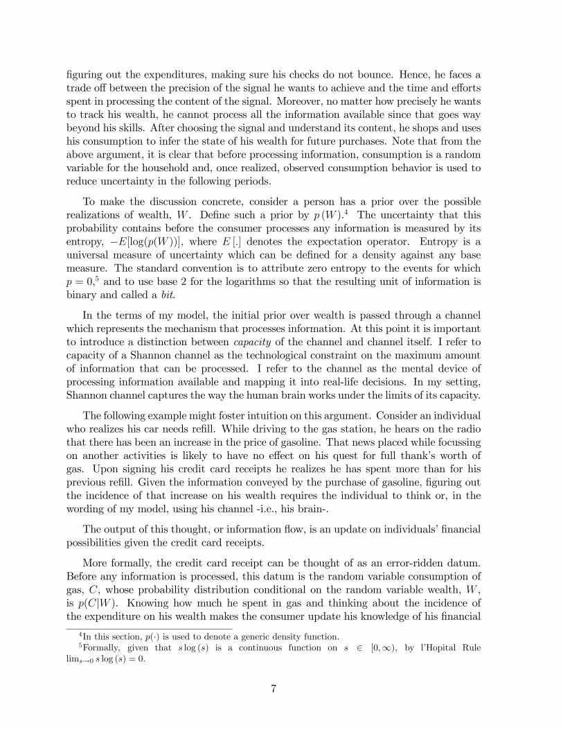
Suppose the household has three wealth possibilities w 2 W � f2; 4; 6g and three con-sumption possibilities c 2 C � f2; 4; 6g. Before any observation is made, the consumerhas the following prior on wealth, Pr (w = 2) = :5, Pr (w = 4) = :25, Pr (w = 6) = :25.Moreover the consumer knows that he cannot borrow, c � w and, if his check bounceshe will have to pay a �ne in terms of consumption c = 0. The utility he derives fromconsumption where utility is de�ned as u (c) � log (c). His payo¤ matrix is summarizedin Figure a.

cnw 2 4 62 0:7 0:7 0:74 �1 1:38 1:386 �1 �1 1:8

Figure a: Payo¤ Matrix with u(c)�log(c)

If uncertainty in the payo¤ can be reduced at no cost, the consumer would set c = 2whenever he knows that w = 2, c = 4 whenever w = 5 and, �nally, c = 6 if w = 8.

In contrast, if there is no possibility of gathering information about wealth besidesthe one provided by the prior, the consumer will avoid in�nite disutility by setting c = 2whatever the wealth. The di¤erence in bits in the two policies is measured by the mutualinformation between C and W . I measure the ex-ante uncertainty embedded in theprior for w by evaluating its entropy in bits, i.e., H (W ) � �

Xw2W

p (w) � log2 (p (w)) =

0:5�log2�10:5

�+0:25�log2

�10:25

�+0:25�log2

�10:25

�= 1:5 bits. Since observation of c provides

information on wealth, conditional on the knowledge of consumption uncertainty aboutw is reduced by the amount H (W jC) �

Xw2W

Xc2C

p (c; w) log2 (p (wj c)). The mutual

information between C and W , i.e., the remaining uncertainty about the wealth afterobserving consumption is the di¤erence between ex-ante uncertainty of W (H (W )) andthe knowledge ofW provided through C (H (W jC)). In formulae, the mutual informationor capacity of the channel amounts to:

MI (C;W ) � H (W )�H (W jC) =

=Xw2W

Xc2C

p (c; w) log

�p (c; w)

p (c) p (w)

�

9

To see what this formula implies in the two cases proposed, consider �rst the situationin which information can �ow at in�nite rate.

First notice that in this case ex-post uncertainty will be fully resolved. Moreover, notethat (p (wj c)) = 1; 8c 2 C; 8w 2 W since the consumer is setting positive probabilityon one and only one value of consumption per value of wealth. This in turns impliesH (W jC) = 0. Thus the mutual information in this case will be MI (C;W ) = H (W ) :

On the other hand, if consumer has zero information �ow or, equivalently, if process-ing information would be prohibitively hard for him, his optimal policy of setting c = 2at all times makes consumption and wealth independent of each other. This implies

that H (W jC) =Xw2W

Xc2C

p (c) p (w) log2

�p(c)p(w)p(c)

�!= H (W ). Hence, in this case

MI (C;W ) = 0 and no reduction in the uncertainty about wealth occurred by ob-serving consumption. This makes intuitive sense. If a consumer decides to spendthe same amount in consumption regardless of his wealth level, his purchase will tellhim nothing about his �nancial possibilities. The expected utility in the �rst case isEFullInfo (u (c)) = (log (2)) � (:5) + (log (4) + log (6)) � (:25) = 1:14 while in the secondcase ENoInfo (u (c)) = 0:7. Now, assume that the consumer can allocate some e¤ort inchoosing size and scope of information about his wealth he wants to process, under thelimits imposed by his processing capacity. Note the occurrence of two elements equallyessential for the rational choice of the consumer. The �rst, limits in processing capac-ity, is a technological constraint: the information �ow that his brain allows is bounded.The second is the interest of the consumer captured by his utility function. A rationalconsumer takes into account his limits and chooses the scope of information about hiswealth accordingly guided by his preferences, u (c).

Given the risk aversion of the consumer and since the consumer has always the optionto set c = 2 and use no capacity, with small but positive information �ow available hewill choose the distribution p (cjw) as dependent on w as his capacity allows him to.

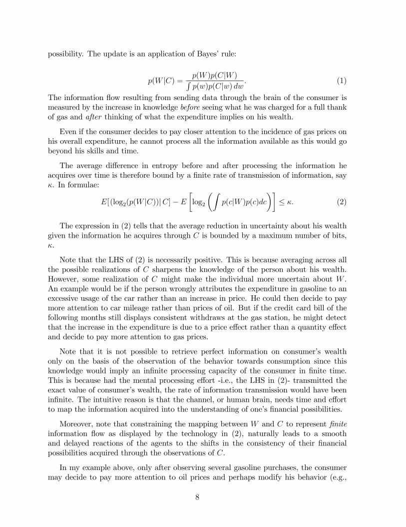
Let �� be the maximum amount of information �ow that the consumer can process.Let the probability matrix of the consumer be described by:

cnw P (w = 2) P (w = 5) P (w = 8)

P (c = 2) 0:5 p1 p2P (c = 4) 0 :25� p1 p3P (c = 6) 0 0 :25� p2 � p3

Figure b: Probability Matrix

where the zero on the South-West corner of the matrix encodes the no borrowing con-straint c � w.

The program of the consumer amounts to:6

maxfp1;p2;p3g

E� (u (c))

6The explicit formulation takes up the form:

10

s.t.�� �MI (C;W ) :

Given �� = 0:3,7 the optimal policy sets p�1 = 0:125; p�2 = 0:125, p3 = 0:125. This

correspond to a mass distribution of Pr (C = c) :

8<:0:75 if c = 20:25 if c = 40:0 if c = 6

, which leads to an

expected utility of E� (u (c)) = 0:87 and a mutual information of MI (C;W ) = �� = 0:3bits . Hence, consumers who invest e¤ort in tracking their wealth using the channel arebetter o¤ than in the no information case -higher expected utility- even though theycannot do as well as in the constrained case.

Note that the result of trading o¤ information on the highest value for more preciseknowledge of lower value of wealth is driven by the choice of utility. For instance, if I hadchosen a consumer with the same bound of processing capacity but higher degree of riskaversion, say one for which u (c) = c1�

1� with = 5, he would have chosen a probabilityPr (C = 2) even higher than his log-utility counterpart. On the other hand, a consumerwith degree of risk aversion = 0:3 would have shift probability mass from Pr (C = 2) toPr (C = 6). The intuition behind this result is that since the attention of the consumerwithin the limits of Shannon capacity is allocated according to his utility, the degree ofrisk aversion plays an important role in choosing the direction of this attention and, inturns, the scope of the signal. A log-utility consumer wants to be well informed aboutmiddle values of his wealth, whether an high risk aversion consumer selects a signal whichprovides sharper information on the lower values of wealth, so that he can avoid �1disutility. The opposite direction is taken by a risk averse agent characterized by = 0:3.

maxfp1;p2;p3g

E� (u (c)) = (log (2)) � (:5 + p1 + p2) +

+ (log (4)) � (:25� p1 + p3) ++ (log (6)) � (:25� p2 � p3)

s.t.

�� � MI (C;W ) =

= :5 log2

�:5

:5 (:5 + p1 + p2)

�+ :p1 log2

�p1

:25 (:5 + p1 + p2)

�+

+p2 log2

�p2

:25 (:5 + p1 + p2)

�+ (:25� p1) log2

�(:25� p1)

:25 (:25� p1 + p3)

�+

+(:25� p2 � p3) log2�

(:25� p2 � p3):25 (:25� p2 � p3)

�:

7Note that such a bound of information �ow is unrealistically low. However I decided to trade o¤realism for simplicity in this example.

11

2.2 The Mathematics of Rational Inattention.

This part addresses the mathematical foundations of rational inattention. The mainreference is the seminal work of Shannon (1948). Drawing from the Information Theoryliterature, I provide an axiomatic characterization of entropy and mutual informationand show the main theoretical features of these two pivotal quantities that set the stagefor a rigorous basis of information theory.

Formally, the starting point is a set of possible events whose probabilities of occurrenceare p1; p2; : : : ; pn. Suppose for a moment that these probabilities are known but that isall we know concerning which event will occur. The quantity H = �

Pi pi log pi is called

the entropy of the set of probabilities p1; : : : ; pn. If x is a chance variable, then H (x)indicates its entropy; thus x is not an argument of a function but a label for a number,to di¤erentiate it from H (y) say, the entropy of the chance variable y.

Quantities of the form H = �P

i pi log pi play a central role in Information Theoryas measures of information, choice and uncertainty. The form of H will be recognizedas that of entropy as de�ned in certain formulations of statistical mechanics8 where pi isthe probability of a system being in cell i of its phase space.

The measure of howmuch choice is involved in the selection of the events isH (p1; p2; ::; pn)and it has the following properties:

Axiom 1 H is continuous in the pi.

Axiom 2 If all the pi are equal, pi = 1n, then H should be a monotonic increasing function of

n. With equally likely events there is more choice, or uncertainty, when there aremore possible events.

Axiom 3 If a choice is broken down into two successive choices, the original H should be theweighted sum of the individual values of H.

Theorem 2 of Shannon (1948) establishes the following results:

Theorem 1 The only H satisfying the three above assumptions is of the form:

H = �KnXi=1

pi log pi

where K is a positive constant that amounts for the choice of the unit measure.

8See, for example, R. C. Tolman, Principles of Statistical Mechanics, Oxford, Clarendon, 1938.

12

Figure c: Entropy of two choices with probability p and q=1�p as function of p:

There are certain distinguished features that make entropy a suitable measure of uncer-tainty.

Remark 1. . H = 0 if and only if all the pi but one are zero, this one having the valueunity. Thus only when we are certain of the outcome does H vanish. Otherwise His positive.

Remark 2. For a given n, H is a maximum and equal to log n when all the pi are equal(i.e., 1

n). This is also intuitively the most uncertain situation.

Remark 3. Suppose there are two random variables, X and Y ,

H(Y ) = �Xx;y

p(x; y) logXx

p(x; y)

Moreover,H(X; Y ) � H(X) +H(Y )

with equality only if the events are independent (i.e., p(x; y) = p(x)p(y)). Thismeans that the uncertainty of a joint event is less than or equal to the sum of theindividual uncertainties.

Remark 4. Any change toward equalization of the probabilities p1; p2; : : : ; pn increasesH. Thus if p1 < p2 an increase in p1, or a decrease in p2 that makes the two probabil-ities more alike results into an increase inH. The intuition is trivial since equalizingthe probabilities of two events makes them indistinguishable and therefore increasesuncertainty on their occurrence. More generally, if we perform any �averaging�op-eration on the pi of the form p0i =

Pj aijpj where

Pi aij =

Pj aij = 1, and all

aij � 0, then in general H increases9.

Remark 5. Given two random variables X and Y as in 3, not necessarily independent,for any particular value x that X can assume there is a conditional probabilitypx(y) that Y has the value y. This is given by

px(y) =p(x; y)Py p(x; y)

:

9The only case in which H remains unchanged is when the transformation results in just one permu-tation of pj .

13

The conditional entropy of Y , is then de�ned asHX(Y ) and amounts to the averageof the entropy of Y for each possible realization the random variable X, weightedaccording to the probability of getting a particular realization x. In formulae,

HX(Y ) = �Xx;y

p(x; y) log px(y):

This quantity measures the average amount of uncertainty in Y after knowing X.Substituting the value of px(y) , delivers

HX(Y ) = �Xx;y

p(x; y) log p(x; y) +Xx;y

p(x; y) logXy

p(x; y)

= H(X; Y )�H(X)

orH(X; Y ) = H(X) +HX(Y ):

This formula has a simple interpretation. The uncertainty (or entropy) of the jointevent X;Y is the uncertainty of X plus the uncertainty of Y after learning the realizationof X.

Remark 6. Combining the results in Axiom 3 and Axiom 5, it is possible to recoverH(X) +H(Y ) � H(X; Y ) = H(X) +HX(Y ):

This reads H(Y ) � HX(Y ) and implies that the uncertainty of Y is never increasedby knowledge of X. If the two random variables are independent, then the entropy willremain unchanged.

To substantiate the interpretation of entropy as the rate of generating information, itis necessary to linkH with the notion of a channel. A channel is simply the medium usedto transmit information from the source to the destination, and its capacity is de�nedas the rate at which the channel transmits information. A discrete channel is a systemthrough which a sequence of choices from a �nite set of elementary symbols S1; : : : ; Sncan be transmitted from one point to another. Each of the symbols Si is assumed to havea certain duration in time ti seconds . It is not required that all possible sequences ofthe Si be capable of transmission on the system; certain sequences only may be allowed.These will be possible signals for the channel. Given a channel, one may be interestedin measuring its capacity of such a channel to transmit information. In general, withdi¤erent lengths of symbols and constraints on the allowed sequences, the capacity of thechannel is de�ned as:

De�nition 2 The capacity C of a discrete channel is given by

C = limT!1

logN(T )

T

where N(T ) is the number of allowed signals of duration T .

14

To explain the argument in a very simple case, consider a telegraph where all symbolsare of the same duration, and any sequence of the 32 symbols is allowed . Each symbolrepresents �ve bits of information. If the system transmits n symbols per second it isnatural to say that the channel has a capacity of 5n bits per second. This does not meanthat the teletype channel will always be transmitting information at this rate � this isthe maximum possible rate and whether or not the actual rate reaches this maximumdepends on the source of information which feeds the channel. The link between channelcapacity and entropy is illustrated by the following Theorem 9 of Shannon:

Theorem 3 Let a source have entropy H (bits per second) and a channel have a capacityC (bits per second). Then it is possible to encode the output of the source in such a way

as to transmit at the average rateC

H � " symbols per second over the channel where " is

arbitrarily small. It is not possible to transmit at an average rate greater thanC

H .

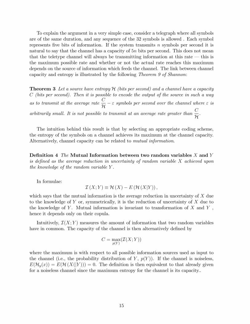
The intuition behind this result is that by selecting an appropriate coding scheme,the entropy of the symbols on a channel achieves its maximum at the channel capacity.Alternatively, channel capacity can be related to mutual information.

De�nition 4 The Mutual Information between two random variables X and Yis de�ned as the average reduction in uncertainty of random variable X achieved uponthe knowledge of the random variable Y .

In formulae:I (X;Y ) � H (X)� E (H (XjY )) ;

which says that the mutual information is the average reduction in uncertainty of X dueto the knowledge of Y or, symmetrically, it is the reduction of uncertainty of X due tothe knowledge of Y . Mutual information is invariant to transformation of X and Y ,hence it depends only on their copula.

Intuitively, I(X;Y ) measures the amount of information that two random variableshave in common. The capacity of the channel is then alternatively de�ned by

C = maxp(Y )

(I(X;Y ))

where the maximum is with respect to all possible information sources used as input tothe channel (i.e., the probability distribution of Y , p(Y )). If the channel is noiseless,E(Hy(x)) = E(H (X(jY ))) = 0. The de�nition is then equivalent to that already givenfor a noiseless channel since the maximum entropy for the channel is its capacity..

15

3 The Formal Set-up

3.1 The problem of the Representative Household

To understand the implications of limits to information processing, let me �rst focus onthe program of on household who can process in�nite amount of information about hiswealth.

Let (;B) be the measurable space where represents the sample set and B theevent set. States and actions are de�ned on (;B). Let It be the ��algebra generatedby fct; wtg up to time t, i.e., It = � (ct; wt; ct�1; wt�1; :::; c0; w0). Then the collectionfItg1t=0 such that It � Is 8s � t is a �ltration. Let u (c) be the utility of the householdde�ned over a consumption good c: I assume that the utility belongs to the CRRA family.

In particular u (c) = c1� t

1� with the coe¢ cient of risk aversion. If the consumer processinformation about his �nancial possibility, he can observe at each time t his wealth, wt.The program in this case amounts to:

maxfctg1t=0

E0

( 1Xt=0

�t��

c1� t

1�

������� I0)

(3)

s.t.wt+1 = R (wt � ct) + yt+1 (4)

ct � wt (5)

w0 given (6)

where � 2 [0; 1) is the discount factor and R = ��1 is the interest on savings (wt � ct).The constraint (5) prevents the household from borrowing. I assume that yt 2 Y ��y1; y2; ::; yN

follows a stationary Markov process with mean Et ((yt+1)j It) = �y:

Assume now that the consumer cannot process all the information available in theeconomy to track precisely his wealth. At time zero, his uncertainty about the wealth issummarized by a prior g (w0) which replaces (6) above.

The consumer can reduce uncertainty about the prior by choosing any joint distribu-tion of consumption and wealth that he can process. That is, the consumer will rationallychoose any distribution that makes p (cjw) as dependent on w as his information process-ing constraint will allow him to. When information cannot �ow at in�nite rate the choiceof the consumer is p (cjw) as opposite to the stream of consumption fctg1t=0 in (3). An-other way of looking at this is that the consumer chooses a noisy signal on wealth wherethe noise distribution-wise can assume any distribution selected by the consumer. Giventhat the agent has a probability distribution over wealth, choosing this signal is akin tochoosing jointly p (c; w). The optimal choice of this distribution is the one that makes thedistribution of consumption conditional on wealth close to wealth under the limits im-posed by Shannon capacity. Hence, the choice of consumption in my setting correspondsto fc (It)g1t=0.

16

Next, I turn to the information constraint. The reduction in uncertainty conveyedby the signal depends on the attention allocated by the consumer to track his wealth.Paying attention to reduce uncertainty requires the consumer to spend some time andutility to process information. I model the arduous task of thinking by appending aShannon channel to the constraints set, and by assuming that the agent associates a costto his e¤ort in terms of utils. Limits in the capacity of the consumers are captured bythe fact that the reduction in uncertainty conveyed by the signal cannot be higher thana given number, ��: The information �ow available to the consumer is described by:

�� � I (Ct;Wt) =

Zp (ct; wt) log

�p (ct; wt)

p (ct) g (wt)

�dctdwt (7)

To describe the way individuals transit across states, de�ne the operatorEwt (Et (xt+1)j ct) �xt+1; which combines the expectation in period t of a variable in period t + 1 with theknowledge of consumption in period t, ct, and the remaining uncertainty over wealth.Applying E to equation (4) leads to:

wt+1 = R (wt � ct) + by (8)

where, note thatby = Ewt (Et (yt+1)j ct)� Ewt (Et ((yt+1)j It)j ct) + [Ewt (Et (yt+1)j ct)� Ewt (Et ((yt+1)j It)j ct)]

LIE= �y + Ewt [(Et (yt+1)j ct)� (Et (yt+1)j ct)]

= �y:

To fully characterize the transition from the prior g (wt) to its posterior distribution,I need to take into account how the choice in time t, p (wt; ct) a¤ects the distributionof consumer�s belief after observing ct:Given the initial prior state g (w0), the successorbelief state, denoted by g0ct (wt+1) is determined by revising each state probability asdisplayed by the expression:

g0�wt+1jct

�=

Z~T (wt+1;wt; ct) p (wtjct) dwt (9)

known as Bayesian conditioning. In (9), the function ~T is the transition function repre-senting (8).

Note that the belief state itself is completely observable. Meanwhile, Bayesian condi-tioning satis�es the Markov assumption by keeping a su¢ cient statistics that summarizesall information needed for optimal control. Thus, (9) replaces (4) in the limited processingworld.

Combining all these ingredients, the program of the household under informationfrictions amounts to

maxfp(wt;ct)g1t=0

E0

( 1Xt=0

�t�c1� t

1�

������ I0)

(10)

17

s.t.

�� � It (Ct;Wt) =

Zp (ct; wt) log

�p (ct; wt)

p (ct) g (wt)

�dctdwt (11)

p (ct; wt) 2 D (w; c) (12)

g0�wt+1jct

�=

Z~T (wt+1;wt; ct) p (wtjct) dwt (13)

g (w0) given (14)

where D (w; c) ��(c; w) :

Rp (c; w) dcdw = 1; p (c; w) � 0;8 (c; w)

in (12) restricts the

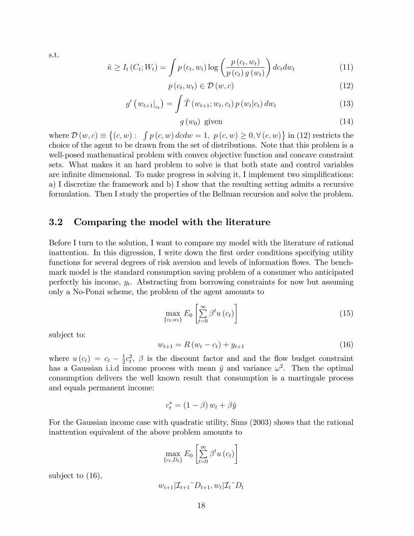
choice of the agent to be drawn from the set of distributions. Note that this problem is awell-posed mathematical problem with convex objective function and concave constraintsets. What makes it an hard problem to solve is that both state and control variablesare in�nite dimensional. To make progress in solving it, I implement two simpli�cations:a) I discretize the framework and b) I show that the resulting setting admits a recursiveformulation. Then I study the properties of the Bellman recursion and solve the problem.

3.2 Comparing the model with the literature

Before I turn to the solution, I want to compare my model with the literature of rationalinattention. In this digression, I write down the �rst order conditions specifying utilityfunctions for several degrees of risk aversion and levels of information �ows. The bench-mark model is the standard consumption saving problem of a consumer who anticipatedperfectly his income, yt. Abstracting from borrowing constraints for now but assumingonly a No-Ponzi scheme, the problem of the agent amounts to

maxfct;wtg

E0

� 1Pt=0

�tu (ct)

�(15)

subject to:wt+1 = R (wt � ct) + yt+1 (16)

where u (ct) = ct � 12c2t , � is the discount factor and and the �ow budget constraint

has a Gaussian i.i.d income process with mean �y and variance !2. Then the optimalconsumption delivers the well known result that consumption is a martingale processand equals permanent income:

c�t = (1� �)wt + ��y

For the Gaussian income case with quadratic utility, Sims (2003) shows that the rationalinattention equivalent of the above problem amounts to

maxfct;Dtg

E0

� 1Pt=0

�tu (ct)

�subject to (16),

wt+1jIt+1~Dt+1; wtjIt~Dt

18

and given w0jI0~Gauss (w0; �20) and

� = 12

�log(R2�2t + !2)� log(�2t+1)

�: :

Given the LQG speci�cation, Sims (2003) shows that the optimal distribution Dt isGaussian with mean wt = Et [wt] and variance �2t = vart (wt).

Note that I assume a constant borrowing constraint, i.e., ct < wt 8t and ct > 0.Therefore, the conventional solution to the benchmark model is no longer correct, norGaussianity of the optimal posterior distribution of consumption and wealth for the ra-tional inattention version of the problem is preserved. The failure of both the martingalesolution for the in the standard model and Gaussianity in the optimal policy of its ratio-nal inattention version is due to the break of the LQ framework implied by the inequalityin the borrowing constraint. In particular in a rational inattention setting, numericalsimulations reveal that preventing excessive borrowing forces to zero some regions ofthe optimal joint distribution of consumption and wealth. Moreover, the support of thedistribution is truncated by the limit on ct.

4 Solution Methodology

4.1 Discretizing the Framework

Let me start by assuming that wealth and consumption are de�ned on compact sects.In particular, admissible consumption pro�les belongs to c � fcmin; :::; cmaxg : Likewise,wealth has support w � fwmin; :::; wmaxg. I identify by j the elements of set c andby i the elements in w: I approximate the state of the problem, i.e., the distribution ofwealth by using the simplex:

De�nition The set � of all mappings g : w ! R ful�lling g (w) � 0 for all w 2 wand

Pw2w

g (w) = 1 is called a simplex. Elements w of w are called vertices of

the simplex �, functions g are called points of �.

Let jSj be the dimension of the belief simplex which approximate the distribution g (w)

and let � �(g 2 RjSj : g (i) � 0 for all i

jSjPi=1

g (i) = 1

)denote the set of all probability

distribution on �. The initial condition for the problem is g (w0) :

The consumer enters each period choosing the joint distribution of consumption and�nancial possibilities. Arguments exactly symmetrical to the ones of the previous sectionlead to specify the control variable for the discretized set up as the probability massfunction Pr (w; c) where c 2 c and w 2 w. This choice of the control variable is alsoconstrained to be drawn from the set of distributions. Given g (w0) and Pr (ct; wt) and

19

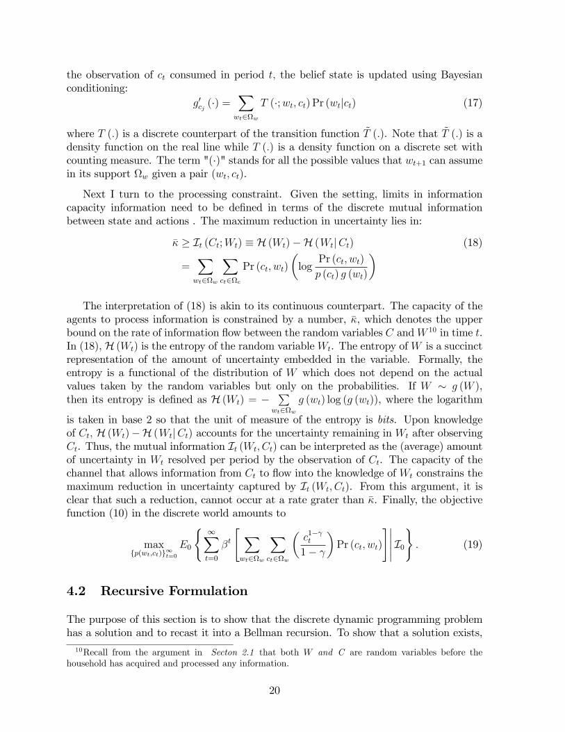
the observation of ct consumed in period t; the belief state is updated using Bayesianconditioning:

g0cj (�) =Xwt2w

T (�;wt; ct) Pr (wtjct) (17)

where T (:) is a discrete counterpart of the transition function ~T (:). Note that ~T (:) is adensity function on the real line while T (:) is a density function on a discrete set withcounting measure. The term "(�)" stands for all the possible values that wt+1 can assumein its support w given a pair (wt; ct).

Next I turn to the processing constraint. Given the setting, limits in informationcapacity information need to be de�ned in terms of the discrete mutual informationbetween state and actions . The maximum reduction in uncertainty lies in:

�� � It (Ct;Wt) � H (Wt)�H (WtjCt) (18)

=Xwt2w

Xct2c

Pr (ct; wt)

�log

Pr (ct; wt)

p (ct) g (wt)

�

The interpretation of (18) is akin to its continuous counterpart. The capacity of theagents to process information is constrained by a number, ��, which denotes the upperbound on the rate of information �ow between the random variables C andW 10 in time t.In (18), H (Wt) is the entropy of the random variableWt. The entropy ofW is a succinctrepresentation of the amount of uncertainty embedded in the variable. Formally, theentropy is a functional of the distribution of W which does not depend on the actualvalues taken by the random variables but only on the probabilities. If W � g (W ),then its entropy is de�ned as H (Wt) = �

Pwt2w

g (wt) log (g (wt)), where the logarithm

is taken in base 2 so that the unit of measure of the entropy is bits. Upon knowledgeof Ct; H (Wt)�H (WtjCt) accounts for the uncertainty remaining in Wt after observingCt. Thus, the mutual information It (Wt; Ct) can be interpreted as the (average) amountof uncertainty in Wt resolved per period by the observation of Ct. The capacity of thechannel that allows information from Ct to �ow into the knowledge of Wt constrains themaximum reduction in uncertainty captured by It (Wt; Ct). From this argument, it isclear that such a reduction, cannot occur at a rate grater than ��. Finally, the objectivefunction (10) in the discrete world amounts to

maxfp(wt;ct)g1t=0

E0

( 1Xt=0

�t

" Xwt2w

Xct2w

�c1� t

1�

�Pr (ct; wt)

#����� I0): (19)

4.2 Recursive Formulation

The purpose of this section is to show that the discrete dynamic programming problemhas a solution and to recast it into a Bellman recursion. To show that a solution exists,10Recall from the argument in Secton 2.1 that both W and C are random variables before the

household has acquired and processed any information.

20

�rst note that the set of constraints for the problem is a compact-valued concave corre-spondence. Second, I need to show that the state space is compact. Compactness comesfrom the assumption of CRRA utility function and the fact that the belief space has abounded support in [0; 1] . Compact domain of the state and the fact that BayesianConditioning for the update preserves the Markovianity of the belief state ensures thatthe transition Q : (w � Y � B ! [0; 1]) and (17) has the Feller property. Then the con-ditions for applying the Theorem of the Maximum in Stockey et al. (1989) are ful�lledwhich guarantees the existence of a solution. In the next section I will provide su¢ cientconditions to guarantee uniqness.

Casting the problem of the consumer in a recursive Bellman equation formulation,the full discrete-time Markov program amounts to:

V (g (wt)) = maxPr(ct;wt)

26664Xwt2w

Xct2c

u (ct) Pr (ct; wt)

!+

+�P

wt2w

Xct2c

V�g0cjt(wt+1)

�Pr (ct; wt)

37775 (20)

subject to:

�� � It (Ct;Wt) =Xwt2w

Xct2c

Pr (ct; wt)

�log

Pr (ct; wt)

p (ct) g (wt)

�(21)

g0cj (�) =Xwt2w

T (�;wt; ct) Pr (wtjct) (22)

Xct2c

Pr (ct; wt) = g (wt) (23)

1 � Pr (ct; wt) � 0 8 (ct; wt) 2 B; 8t (24)

where B � f(ct; wt) : wt � ct; 8ct 2 c;8wt 2 w, 8tg :

The Bellman equation in (20) takes up as argument the marginal distribution of wealthg (wt) and uses as control variable the joint distribution of wealth and consumption,Pr (ct; wt). The latter links the behavior of the agent with respect to consumption (c),on one hand, and income (w) on the other, hence specifying the actions over time. The�rst term on the right hand side of (20) is the utility function u (:) which is assumedto be of the CRRA family with coe¢ cient of risk aversion > 0. The second term,Pwt2w

Xct2c

V�g0cjt(wt+1)

�Pr (ct; wt), represents the expected continuation value of being

in state g (:) discounted by the factor � 2 (0; 1). The expectation is taken with respect tothe endogenously chosen distribution Pr (ct; wt). I have discussed at lenght the relationsin (21)-(24) earlier. Moreover, I appended the equation in (23) which constraints thechoice of the distribution to be consistent with the initial prior g (wt) : Before turningto the optimality conditions that characterize the solution to the problem (20)-(24), Iwill �rst analyze the main properties of the Bellman recursion (20) and derive conditionsunder which is a contraction mapping and show that the mapping is isotone.

21

4.3 Properties of the Bellman Recursion

De�nitions. To prove that the value function is a contraction and isotonic map-ping, I shall introduce the relevant de�nitions. Let me restrict attention to choices ofprobability distributions that satisfy the constraints (21)-(24).To make the notation morecompact, let p � Pr (cjjwi), 8cj 2 c, 8wi 2 w and let � be the set that contains (21)-(24).

D1. A control probability distribution p � Pr (ci; wj) is feasible for the problem (20)-(24) if p 2 �: Let jW j be the cardinality of w and let

G �

8<:g 2 RjW j : g (wi) � 0; 8i;jW jXi=1

g (wi) = 1

9=;denote the set of all probability distributions on w. An optimal policy has a valuefunction that satis�es the Bellman optimality equation in (20):

V � (g) = maxp2�

"Xw2w

Xc2c

u (c) p (cjw)!g (w) + �

Xw2w

Xc2c

(V � (g0c (�))) p (cjw) g (w)#

(25)The Bellman optimality equation can be expressed in value function mapping form.Let V be the set of all bounded real-valued functions V on G and let h : G �w �(w � c)� V ! R be de�ned as follows:

h (g; p; V ) =Xw2w

Xc2c

u (c) p (cjw)!g (w) + �

Xw2w

Xc2c

(V (g0c (�))) p (cjw) g (w) :

De�ne the value function mapping H : V ! V as (HV ) (g) = maxp2� h (g; p; V ).

D2. A value function V dominates another value function U if V (g) � U (g) for allg 2 G:

D3. A mapping H is isotone if V , U 2 V and V � U imply HV � HU:

D4. A supremum norm of two value functions V , U 2 V over G is de�ned as

jjV � U jj = maxg2G

jV (g)� U (g)j

D5. A mapping H is a contraction under the supremum norm if for all V , U 2 V,

jjHV �HU jj � � jjV � U jj

holds for some 0 � � < 1:

22

Next, I prove that the value function recursion is an isotonic contraction. From theseresults, it follows that this recursion converges to a single �xed point corresponding tothe optimal value function V �.

These theoretical results establish that in principle there is no barrier in de�ning valueiteration algorithms for the Bellman recursion under rational inattention. All the proofsare in appendix A.

Uniqueness of the solution to which the value function converges to requires concavityof the constraints and convexity of the objective function. It is immediate to see that allthe constraints but (18) are actually linear in p (c; w) and g (w). For (18), the concavityof p (c; w) is guaranteed by Theorem (16.1.6) of Thomas and Cover (1991). Concavity ofg (w) is the result of the following:

Lemma 1. For a given p (cjw) ; the expression (18) is concave in g (w).

Proof. See Appendix B.

Next, I need to prove convexity of the value function and the fact that the valueiteration is contraction mapping.

Proposition 1. For the discrete Rational Inattention Consumption Saving value recur-sion H and two given functions V and U , it holds that

jjHV �HU jj � � jjV � U jj ;

with 0 � � < 1 and jj:jj the supreme norm. That is, the value recursion H is acontraction mapping.

Proposition 1 can be explained as follows. The space of value functions de�nes avector space and the contraction property ensures that the space is complete. Therefore,the space of value functions together with the supreme norm form a Banach space andthe Banach �xed-point theorem ensures (a) the existence of a single �xed point and (b)that the value recursion always converges to this �xed point (see Theorem 6 of Alvarezand Stockey, 1998 and Theorem 6.2.3 of Puterman, 1994).

Corollary For the discrete Rational Inattention Consumption Saving value recursion Hand two given functions V and U , it holds that

V � U =) HV � HU

that is the value recursion H is an isotonic mapping.

The isotonic property of the value recursion ensures that the value iteration convergesmonotonically.

23

5 Optimality Conditions

In this section I incorporate explicitly the constraint on information processing and derivethe Euler Equations that characterize its solution.

The main feature of this section is to relate the link between the output of the channel-consumption- with the capacity chosen by the agent. In deriving the optimality con-ditions, I incorporate the consistency assumption (23) in the main diagonal of the jointdistribution to be chosen, Pr t (cj; wi). Note that such a restriction is WLOG.

5.1 First Order Conditions

To evaluate the derivative of the Bellman equation with respect to a generic distrib-ution Pr (ck1 ; wk2), de�ne the di¤erential operator �kv (l) � v (lk1) � v (lk2) and � asthe shadow cost of processing information: Then, the optimal control for the program(20)-(24) amounts to:

@p� (ck1 ; wk2) :

�ku (c) + ��kV (g0c (:)) = p� (ck1 ; wk2)

���ku

0 (c) �p� (wk2jck1)� ��kV0p� (g

0c (:))

�(26)

This expression states that the optimal distribution depends on the weighted di¤er-ence of two consumption pro�les, ck1 and ck2 where the weights are given by current andfuture discounted utilities. Note that the di¤erential of the marginal utility of currentconsumption is also weighted by the conditional optimal distribution of consumption andwealth.

The interpretation of (26) is that the consumer allocates probabilities by trading-o¤current and future. utilities levels between two consumption pro�les, feasible given hisprior on wealth, with the corresponding intertemporal di¤erence in marginal utilities. Toillustrate the argument, suppose a consumer believes that his wealth is wk2 with highprobability. Suppose for simplicity that wk2 allows him to spend ck1 or ck2. The decisionof shifting probability from p (ck2 ; wk2) to p (ck1 ; wk2) depends on four variables. First,the current di¤erence in utility levels, �ku (c) which tells the immediate satisfaction ofconsuming ck1 rather than ck2. However, consuming more today has a cost in futureconsumption and wealth levels tomorrow, ��kV (g

0c (:)). This is not the end of the story.

Optimal allocation of probabilities requires trading o¤ not only intertemporal levels ofutility but also marginal intertemporal utilities where now the current marginal utilityof consumption is weighted by the e¤ort required to process information today.

To explore this relation further, I evaluate the derivative of the continuation value fora given optimal p� (ck1 ; wk2), that is �kV

0p� (g

0c (:)). To this end, de�ne the ratio between

di¤erential in utilities (current and discounted future) and di¤erential in marginal currentutility as � � �ku(c(�))+��kV (g

0c(:))

��[u0(ck1 (�))�u0(ck2 (�))]. Also, let �� be the ratio � when current level of

utilities are equalized and future di¤erential utilities are constant, i.e., �ku (c) = 0 and

24

�kV (g0c (:)) = 1 or, �

� � �

��[u0(ck1 (�))�u0(ck2 (�))]. Then, an application of Chain rule and

point-wise di¤erentiation leads to

p� (ck1 ; wk2) = � (k1; k2) p� (ck1) (27)

where

� (k1; k2) � �1 (�; p� (ck1 ; wk2))��2���; g0ck1

(�) ; p� (ck1 ; wk2)���3���; g0ck2

(�) ; p� (ck1 ; wk2)�

The details of the derivation of (43) are in Appendix C. Here I focus on the expla-nation for the terms � (k1; k2) which characterize the optimal solution of the conditionaldistribution p� (wk2jck1) :

The �rst term �1 (�; p� (ck1 ; wk2)) � e

0B@ �

p�(ck1 ;wk2)

1CAstates that the optimal choice

of the distribution balances di¤erentials between current and future levels of utilitiesbetween high (k2) and low (k1) values of consumption. In case of log utility, the termexp (�) is a likelihood ratio between utilities in the two states of the word (k1 and k2) andthe interpretation is that the higher is the value of the state of the world k2 with respectto k1 as measured by the utility of consumption, the lower is the optimal p� (ck1 ; wk2).This matches the intuition since the consumer would like to place more probability onthe occurrence of k2 the wider the di¤erence between ck1 and ck2. A perhaps moreinteresting intertemporal relation is captured by the terms �2 and �3, both of whichdisplay the occurrence of the update distribution g0cki (�), i = 1; 2. To disentangle thecontribution of each argument of �2 and �3, I combine the derivative of the control withthe envelope condition. Let �01 be the term �1 led one period and de�ne the di¤erentialbetween transition from one particular state to another and transition from one particular

state to all the possible states as ~�Tj � T��;wk2 ; ckj

���P

i

T (�;wi; ck1) p��wijckj

��for

j = 1; 2. Evaluating the derivative with respect to the state almost surely reveals that

�2 � exp

���� �01

p(ck1)~�T1

�while �3 � exp

���� �01

p(ck2)~�T2

�. The terms �2 and �3

reveal that in setting the optimal distribution p� (ck1 ; wk2) consumers take into accountnot only di¤erential between levels and marginal utilities but also how the choice of thedistribution shrinks or widens the spectrum of states that are reachable after observingthe realized consumption pro�le.

An interesting special case that admits a close form solution is when the agent isrisk neutral. Consider the framework in Section (3.2) and let utility take up the formu (c) = ct, then in the region of admissible solution ct < wt, the optimal probabilitydistribution makes c independent on w. To see this, it is easy to check that in the twoperiod case with no discounting, the utility function reduces to u (c) = w, which impliescjw / U (wmin; wmax). That is, since all the uncertainty is driven by w, the consumerdoes not bother processing information beyond the knowledge of where the limit of c = wlies. In other word, the constraint on information �ow does not bind. With continuation

25

value, exploiting risk neutrality, the optimal policy function amounts to:

p� (wk2jck1) =e

[(ck1�ck2)+��k �V (g

0c(:))]

�

!Pj

~�Tj(28)

The solution uncovers some important properties of the interplay between risk neutralityand information �ow. First of all, households with linear utility do not spend extraconsumption units in sharpening their knowledge of wealth. This is due to the fact thatsince the consumer is risk neutral and, at the margin, costs and bene�ts of information�ows are equalized amongst periods, there is no necessity to gather more informationthan the boundaries of current consumption possibilities. In each period, the presence ofinformation processing constraint forces the consumer to allocate some utils to learn justenough to prevent violating the non-borrowing constraint. Once those limits are �guredout, consumption pro�les in the region c < w are independent on the value of wealth.

Another special case that admits close form soluition when consumers are risk averseand have information-processing limits is the 3 � points distribution illustrated in Ap-pendix D.

6 Numerical Technique and its Predictions

I solve the discrete dynamic rational inattention consumption-saving model is to trans-form the underlying partially observable Markov decision process into an equivalent, fullyobservable, Markov decision process with a state space that consists of all probabilitydistributions over the core states of the model (i.e., wealth) and solve it using dynamicprogramming.

For a model with n cores states, w1; ::; wn, the transformed state space is the (n� 1)-dimensional simplex, or belief simplex. Expressed in plain terms, a belief simplex is apoint, a line segment, a triangle or a tethraedon in a single, two, three or four-dimensionalspace, respectively. Formally, a belief simplex is de�ned as the convex hull11 of beliefstates from an a¢ nely independent12 set B. The points of B are the vertices of the beliefsimplex. The convex hull formed by any subset of B is a face of the belief simplex. Toaddress the issue of dimensionality in the state space of my model, I use a grid-basedapproximation approach. The idea of a grid based approach is to use a �nite grid todiscretize the continuous state space which is uncountably in�nite. The implementationamounts to: I place a �nite grid over the simplex point, I compute the values for pointsin the grid, and I use interpolation to evaluate all other points in the simplex.

In the following subsections I will �x some de�nitions, describe the techniques indetails and discuss the results.11A convex hull of a set of points is de�ned as the closure of the set under convex combination.12A set of belief states fgig, 1 � i � jSj is called a¢ nely independent when the vectors

�gi � gjSj

are

linearly independent for 1 � i � jSj.

26

6.1 Belief Simplex and Dynamic Programming

As mentioned previously, if I were to model wealth as the state of a Markov systemdirectly accessible to the consumer, previous history of the process would be irrelevantto its optimal control. However, since the consumer does not know or cannot completelyobserve wealth, he may require all the past information about the system to behaveoptimally. The most general approach is to keep track of the entire history of his previousconsumption purchases up to time t, denoted Ht = fg0; c1; ::; ct�1g. For any given initialstate probability distribution g0, the number of possible histories is (jCj)t with C denotingthe set of consumption behavior up to time t. This number goes to in�nity as thedecision horizon approaches in�nity, which makes this method of representing the historyuseless for in�nite-horizon problems. To overcome this issue, Astrom (1965) proposed aninformation state approach. The latter is based upon the idea that all the informationneeded to act optimally can be summarized by a vector of probabilities over the system,called belief state. Let g (w) denote the probability that the wealth is in state w 2 wwhere w is assumed to be a �nite set. Probability distributions such as g (w) de�nedon �nite sets can be looked up as simplex. The following de�nitions provide the formalbasis for the construction of the grid for the simplex of the state.

Recall that jSj is the dimension of the belief simplex which approximates the distribu-

tion g (w) andG �(g 2 RjSj : g (i) � 0 for all i

jSjPi=1

g (i) = 1

)is the set of all probability

distribution on the simplex.

The discretization of the core states and the belief states amount to an equi-spacedgrid with n = 6; 7; 8 values for w ranging from 1 to n i.e., w 2 w � fw1; ::; wngand jSj � 8; 9 and 10 distinct values for the marginal pdf g (w) in the interval I� �[0; 1]. Hence, the simplex result into a 1296x6 matrix for (n; jSj) = (f6g ; f10g), 3003x7matrix for (n; jSj) = (f7g ; f9g) and, �nally 11364x8 matrix for (n; jSj) = (f8g ; f10g).Given the initial belief simplex, its successor belief states can be determined by usingBayesian conditioning at each multidimensional point of the simplex and amounts to theexpression:

g0c (�) =Xi

Xj

T (�;wi; cj) Pr (wijcj) = Pr (�jc) : (29)

Next, let me turn to the action space. Imposing the constraint that consumption cannotexceed wealth in each period, that is ct < wt, 8t, I perform the discretization of thebehavior space in a fashion similar to the core states, that is an equi-spaced grid where c =13w. As a result, the behavior space is the compact set c � fc1; ::; cng =

�13w1; ::;

13wn.

Let core states and behavior states be sorted in descending order. Then, given thesymmetry in the dimensionality of core space and behavior space and the constraint c <w, the the joint distribution of consumption and wealth for a given multidimensional pointon the grid of the simplex is a square matrix with rows correspond to levels of consumptionand summing the matrix per row returns the marginal distribution of consumption, p (c).Likewise, the columns of the matrix correspond to levels of wealth. Evaluating the sumper columns of the matrix amounts to the marginal pdf of wealth, g (w). Let V be the

27

set of all bounded real-valued function V on G. Then the Bellman optimality equationof the household amounts to:

V (g (W )) = maxPr (cj ;wi)

( Pi

Pj u (cj) Pr (cj; wi)+

+�nP

i

Pj V�g0cj (�)

�Pr (cj; wi)

o )s.t

� = I (C;W ) =Xi

Xj

Pr (cj; wi) log

�Pr (cj; wi)

p (cj) g (wi)

�

Without loss of generality, I place the restriction that the columns of the matrixPr (cj; wi) need to sum to the marginal pdf of wealth in the main diagonal. Moreover,since some of the values of the marginal g (w) per simplex-point are exactly zero given thede�nition of the envelope for the simplex, I constrain the choices of the joint distributionscorresponding to those values to be zero. This handling of the zeros makes the parametervector being optimized over have di¤erent lengths for di¤erent rows of the simplex . Hencethe degrees of freedom in the choice of the control variables for simplex points vary froma minimum of 0 to a maximum of n�(n�1)

2.13 Once the belief simplex is set up, I initialize

the joint probability distribution of consumption and wealth per belief point and solvethe program of the household by backward induction iterating on the value functionV (g (W )). I evaluate the value function that takes as argument the updated distribution

of the wealth in (29), i.e., V�g0cj (�)

�using linear interpolation.

A linear interpolant approximates the exact non linear value function in (20) with apiece-wise linear function. The following propositions illustrate this point.

Proposition 2. If the utility is CRRA and if Pr (cj; wi) satisfying (21)-(24), then theoptimal n� step value function Vn (g) de�ned over G can be expressed as:

Vn (g) = maxf�ingi

Xi

�n (wi) g (wi)

where the �� vectors, � : w ! R, are jW j �dimensional hyperplanes.

Intuitively, each �n�vector corresponds to a plan and the action associated with agiven �n�vector is the optimal action for planning horizon n for all priors that have such13To illustrate this point, two example in which the 0-degree of freedom and the n�(n�1)

2 -degree offreedom occur are as follows. Suppose for simplicity that n = 3: Then, if a simplex point has realization

g � f1; 0; 0g the joint pdf of consumption and wealth turns out to be p (c; w) =

24 1 0 00 00

35 leavingzero degrees of freedom. If, instead, e.g., g �

�13 ;

13 ;

13

, the consumers has to choose 3�(2)

2 = 3 points onthe joint distribution, fp1; p2; p3g placed as:

p (c; w) =

24 13 p1 p2

13 p3

13

35 :28

a function as the maximizing one. With the above de�nition, the value function amountsto:

Vn (g) = maxf�ingi

�in; g

�;

and thus the proposition holds.

Using the above proposition and the fact that the set of all consumption pro�lesP � fc < w : p (c) > 0g is discrete, it is possible to show directly the convex propertiesfor the Value Function. For �xed �in�vectors, h�in; gi operator is linear in the belief space. Therefore the convex property is given by the fact that Vn is de�ned as the maximumof a set of convex (linear) functions and, thus, obtains a convex function as a result.The optimal value function, V �, is the limit for n!1 and, since all the Vn are convexfunction, so is V �.

Proposition 3. Assuming CRRA utility function and under the conditions of Proposi-tion 1, let V0 be an initial value function that is piecewise linear and convex. Thenthe ith value function obtained after a �nite number of update steps for a RationalInattention Consumption-Saving problem is also �nite, piecewise linear and convex(PCWL).

To implement numerical the optimization of the value function at each point of thesimplex, I use a via gradient-based search methods using Chris Sims�s csminwel anditerate on the value function up to convergence.

Finally, I draw from the optimal policy function -i.e., ergodic posterior joint distribu-tion of consumption and wealth, p� (c; w) - and generate time series path of consumption,wealth and expected wealth evaluated by combing the core states with the posterior dis-tribution of wealth which results from the optimization. Moreover I use the joint posteriorp� (c; w) to draw the time path of Information Flow (��t �

Pi

Pj p

�t (cj; wi) log

�p�t (cj ;wi)

p�t (cj)g�t (wi)

�).

A pseudocode that implements the procedure is in Appendix E.

7 Results

In this section, by varying the shadow cost of information �ow and utility speci�-cations, I investigate the dynamic interplay of information �ows and degrees of riskaversion. In particular, I study three di¤erent models where each model is character-ized by a given processing e¤ort, �; and di¤erent degrees of risk aversion, ; where = (f7g ; f5g ; f3g ; f0g ; f0:5g ; f0:3g).

The patterns that emerge are the following.

Result 1. Restricted Support The optimal policy function for the information-constrainedconsumer places low weight, even zero, on low values of consumption for high valuesof wealth. This e¤ect is more pronounced the higher the information �ow.

29

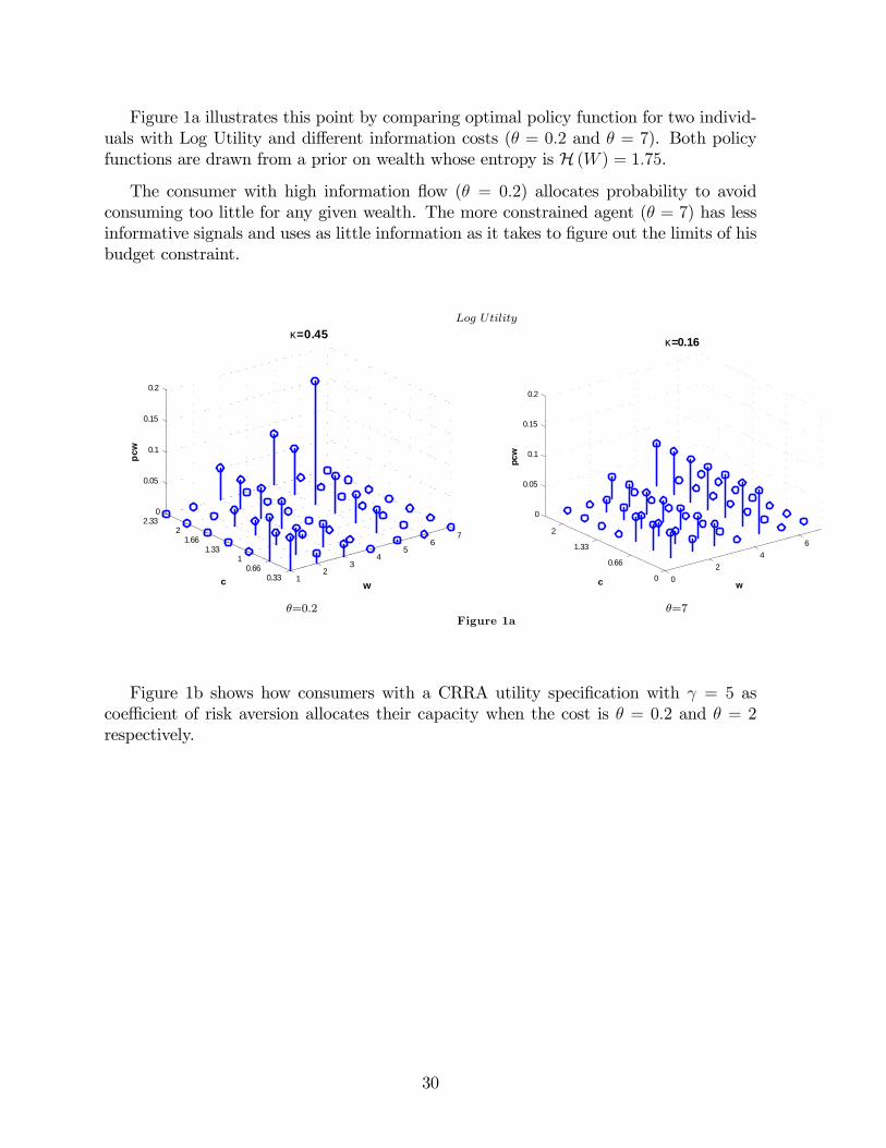
Figure 1a illustrates this point by comparing optimal policy function for two individ-uals with Log Utility and di¤erent information costs (� = 0:2 and � = 7). Both policyfunctions are drawn from a prior on wealth whose entropy is H (W ) = 1:75.

The consumer with high information �ow (� = 0:2) allocates probability to avoidconsuming too little for any given wealth. The more constrained agent (� = 7) has lessinformative signals and uses as little information as it takes to �gure out the limits of hisbudget constraint.

Log Utility

12

34

56

7

0.330.66

11.33

1.662

2.330

0.05

0.1

0.15

0.2

w

κ=0.45

c

pcw

�=0:2

02

46

0

0.66

1.33

2

0

0.05

0.1

0.15

0.2

w

κ=0.16

c

pcw

�=7Figure 1a

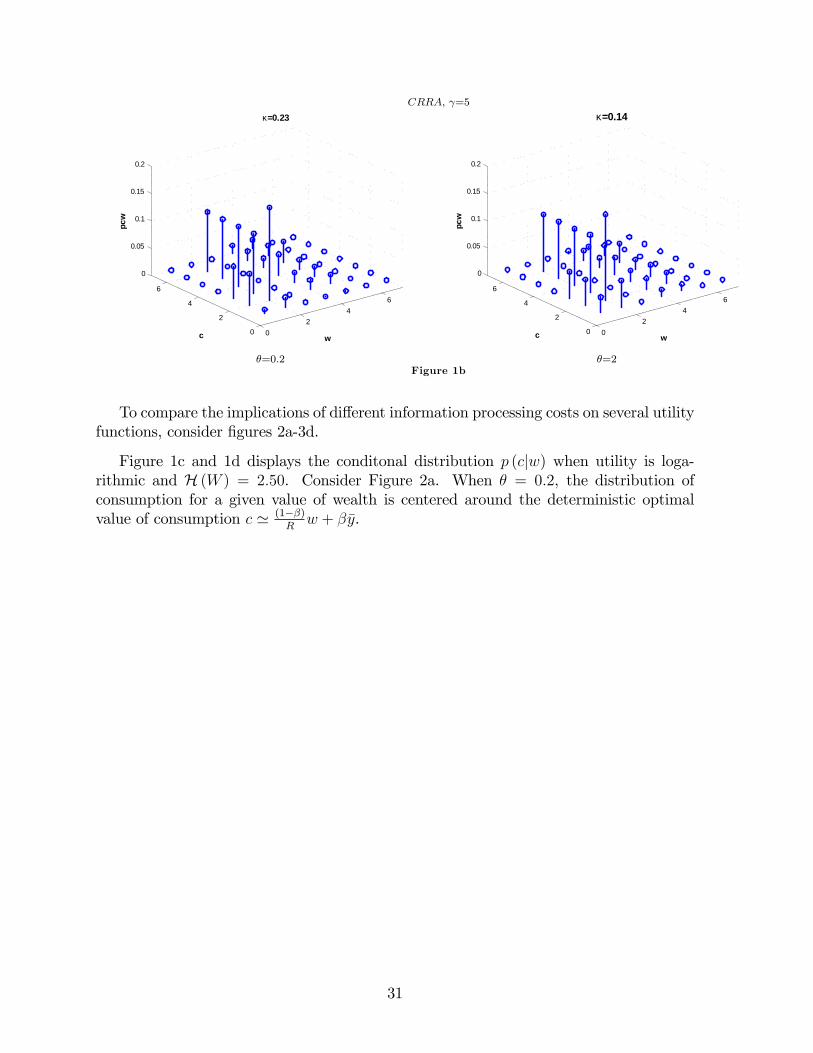
Figure 1b shows how consumers with a CRRA utility speci�cation with = 5 ascoe¢ cient of risk aversion allocates their capacity when the cost is � = 0:2 and � = 2respectively.

30

CRRA; =5

02

46

0

2

4

6

0

0.05

0.1

0.15

0.2

w

κ=0.23

c

pcw

�=0:2

02

46

0

2

4

6

0

0.05

0.1

0.15

0.2

w

κ=0.14

c

pcw

�=2Figure 1b

To compare the implications of di¤erent information processing costs on several utilityfunctions, consider �gures 2a-3d.

Figure 1c and 1d displays the conditonal distribution p (cjw) when utility is loga-rithmic and H (W ) = 2:50. Consider Figure 2a. When � = 0:2, the distribution ofconsumption for a given value of wealth is centered around the deterministic optimalvalue of consumption c ' (1��)

Rw + ��y.

31

Log Utility; �=0:2

0.33 0.66 1.00 1.33 1.66 2.00 2.330

0.1

0.2

0.3

0.4

0.5

0.6

0.7p(c|w=1)

0.33 0.66 1.00 1.33 1.66 2.00 2.330

0.1

0.2

0.3

0.4

0.5

0.6

p(c|w=2)

0.33 0.66 1.00 1.33 1.66 2.00 2.330

0.1

0.2

0.3

0.4

0.5

0.6

p(c|w=4)

0.33 0.66 1.00 1.33 1.66 2.00 2.330

0.1

0.2

0.3

0.4

0.5

0.6

p(c|w=5)

Figure 1c

Figure 1c shows what happens when information is costly. The probability distribu-tion of consumption conditional on wealth is uniform over a range of c for given valuesof wealth. In particular, since information �ows at a very low rate, any value of wealthreveals a much more disperse distribution of consumption for a � = 7-type than a � = 0:2-type.

32

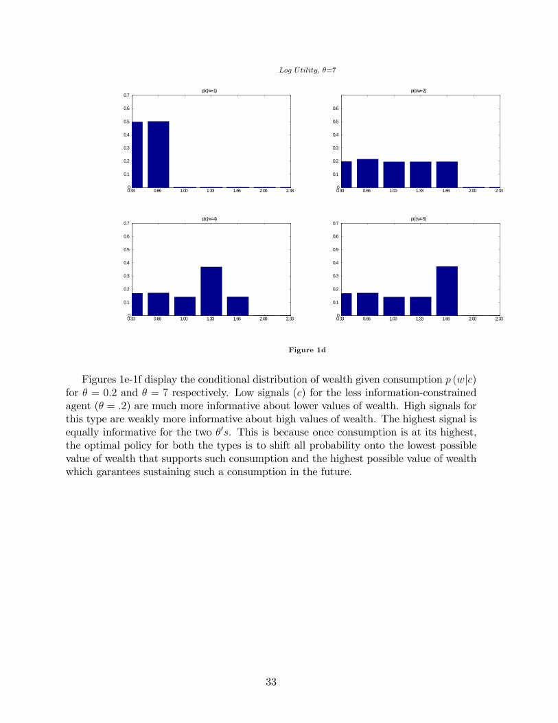
Log Utility; �=7

0.33 0.66 1.00 1.33 1.66 2.00 2.330

0.1

0.2

0.3

0.4

0.5

0.6

0.7p(c|w=1)

0.33 0.66 1.00 1.33 1.66 2.00 2.330

0.1

0.2

0.3

0.4

0.5

0.6

p(c|w=2)

0.33 0.66 1.00 1.33 1.66 2.00 2.330

0.1

0.2

0.3

0.4

0.5

0.6

0.7p(c|w=4)

0.33 0.66 1.00 1.33 1.66 2.00 2.330

0.1

0.2

0.3

0.4

0.5

0.6

0.7p(c|w=5)

Figure 1d

Figures 1e-1f display the conditional distribution of wealth given consumption p (wjc)for � = 0:2 and � = 7 respectively. Low signals (c) for the less information-constrainedagent (� = :2) are much more informative about lower values of wealth. High signals forthis type are weakly more informative about high values of wealth. The highest signal isequally informative for the two �0s. This is because once consumption is at its highest,the optimal policy for both the types is to shift all probability onto the lowest possiblevalue of wealth that supports such consumption and the highest possible value of wealthwhich garantees sustaining such a consumption in the future.

33

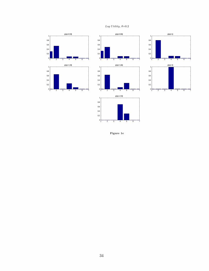
Log Utility; �=0:2

1 2 3 4 5 6 70

0.2

0.4

0.6

0.8

1p(w|c=0.33)

1 2 3 4 5 6 70

0.2

0.4

0.6

0.8

1p(w|c=0.66)

1 2 3 4 5 6 70

0.2

0.4

0.6

0.8

1p(w|c=1)

1 2 3 4 5 6 70

0.2

0.4

0.6

0.8

1p(w|c=1.33)

1 2 3 4 5 6 70

0.2

0.4

0.6

0.8

1p(w|c=1.66)

1 2 3 4 5 6 70

0.2

0.4

0.6

0.8

1p(w|c=2)

1 2 3 4 5 6 70

0.2

0.4

0.6

0.8

1p(w|c=2.33)

Figure 1e

34

Log Utility; �=7

1 2 3 4 5 6 70

0.1

0.2

0.3

0.4

0.5

0.6

0.7p(w|c=0.33)

1 2 3 4 5 6 70

0.1

0.2

0.3

0.4

0.5

0.6

0.7p(w|c=0.66)

1 2 3 4 5 6 70

0.2

0.4

0.6

0.8p(w|c=1)

1 2 3 4 5 6 70

0.1

0.2

0.3

0.4

0.5

0.6

0.7p(w|c=1.33)

1 2 3 4 5 6 70

0.1

0.2

0.3

0.4

0.5

0.6

0.7p(w|c=1.66)

1 2 3 4 5 6 70

0.1

0.2

0.3

0.4

0.5

0.6

0.7p(w|c=2)

1 2 3 4 5 6 70

0.1

0.2

0.3

0.4

0.5

0.6

0.7p(w|c=2.33)

Figure 1f

Figure 1g and 1h display the optimal policy function with CRRA utility speci�cationwith coe¢ cient of risk aversion = 5 and � = 0:2 and � = 2 repsectively. The initial

35

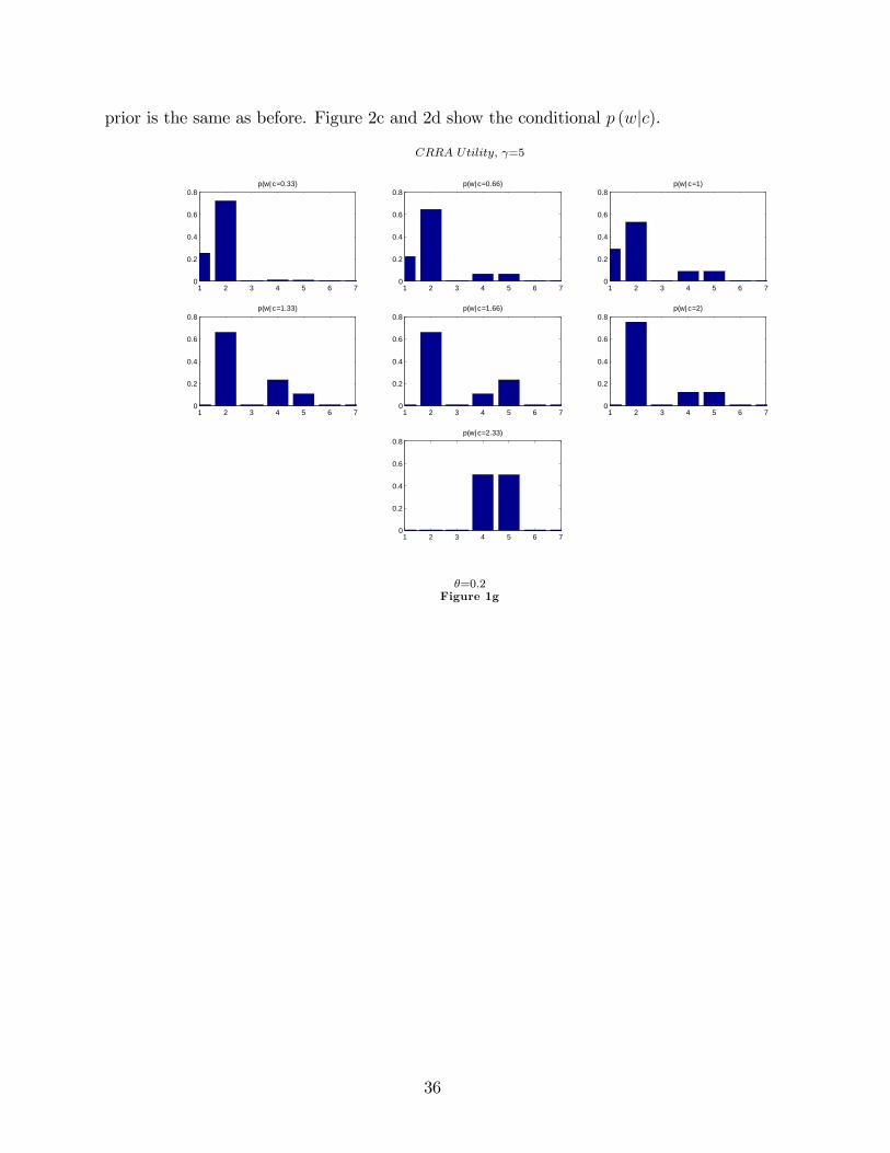
prior is the same as before. Figure 2c and 2d show the conditional p (wjc).

CRRA Utility; =5

1 2 3 4 5 6 70

0.2

0.4

0.6

0.8p(w| c=0.33)

1 2 3 4 5 6 70

0.2

0.4

0.6

0.8p(w| c=0.66)

1 2 3 4 5 6 70

0.2

0.4

0.6

0.8p(w| c=1)

1 2 3 4 5 6 70

0.2

0.4

0.6

0.8p(w| c=1.33)

1 2 3 4 5 6 70

0.2

0.4

0.6

0.8p(w| c=1.66)

1 2 3 4 5 6 70

0.2

0.4

0.6

0.8p(w| c=2)

1 2 3 4 5 6 70

0.2

0.4

0.6

0.8p(w| c=2.33)

�=0:2Figure 1g

36

CRRA Utility; =5

1 2 3 4 5 6 70

0.2

0.4

0.6

0.8p(w| c=0.33)

1 2 3 4 5 6 70

0.1

0.2

0.3

0.4

0.5

0.6

0.7p(w| c=0.66)

1 2 3 4 5 6 70

0.1

0.2

0.3

0.4

0.5

0.6

0.7p(w| c=1)

1 2 3 4 5 6 70

0.1

0.2

0.3

0.4

0.5

0.6

0.7p(w| c=1.33)

1 2 3 4 5 6 70

0.1

0.2

0.3

0.4

0.5

0.6

0.7p(w| c=1.66)

1 2 3 4 5 6 70

0.2

0.4

0.6

0.8p(w| c=2)

1 2 3 4 5 6 70

0.2

0.4

0.6

0.8p(w| c=2.33)

�=2Figure 1h

Figure 1i and 1j plots the corresponding p (cjw) for the risk averse consumer.

37

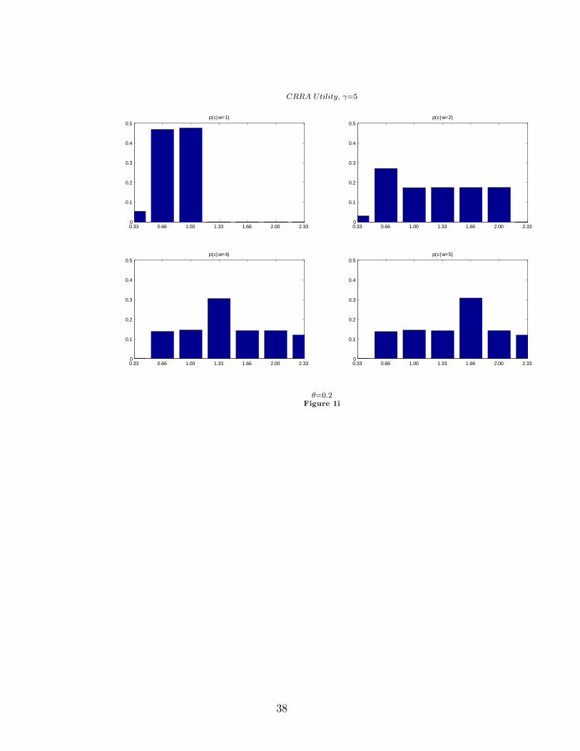
CRRA Utility; =5

0.33 0.66 1.00 1.33 1.66 2.00 2.330

0.1

0.2

0.3

0.4

0.5p(c| w=1)

0.33 0.66 1.00 1.33 1.66 2.00 2.330

0.1

0.2

0.3

0.4

0.5p(c| w=2)

0.33 0.66 1.00 1.33 1.66 2.00 2.330

0.1

0.2

0.3

0.4

0.5p(c| w=4)

0.33 0.66 1.00 1.33 1.66 2.00 2.330

0.1

0.2

0.3

0.4

0.5p(c| w=5)

�=0:2Figure 1i

38

CRRA Utility; =5

0.33 0.66 1.00 1.33 1.66 2.00 2.330

0.05

0.1

0.15

0.2

0.25

0.3

0.35

0.4p(c| w=1)

0.33 0.66 1.00 1.33 1.66 2.00 2.330

0.05

0.1

0.15

0.2

0.25

0.3

0.35

0.4p(c| w=2)

0.33 0.66 1.00 1.33 1.66 2.00 2.330

0.05

0.1

0.15

0.2

0.25

0.3

0.35

0.4p(c| w=4)

0.33 0.66 1.00 1.33 1.66 2.00 2.330

0.05

0.1

0.15

0.2

0.25

0.3

0.35

0.4p(c| w=5)

�=2Figure 1j

Result 2. Information Flow and Risk Aversion In the discrete Rational Inatten-tion Consumption-Saving model, the lower the optimal information �ow, the loweris consumption. Moreover, when the cost of using the channel increases, more riskaverse consumers pay more attention to decreasing the volatility of consumptionrather than to increasing its mean.

The results are documented in Tables 1a-1c. The intuition goes as follows. If process-ing information is relatively easy, i.e., information �ow is large, then a risk averse con-sumer would spend his capacity in having both higher mean and lower variance of con-sumption throughout his life. However, when information processing becomes costly, theconsumer would trade o¤ information about the mean of the consumption for a reductionin its volatility.

The second result comes from evaluating the relation of the value function in steadystate with the expected value of wealth.

Result 3. Optimal Value and Expected Wealth In the discrete Rational Inatten-tion Consumption-Saving model, the �xed-point solution of the value function, V � (g� (w)) ;is positively related with the expected wealth, E� (w) �

Piwig

� (wi) evaluated underthe ergodic distribution of the posterior for wealth. Moreover:

39

1. For a given degree of risk aversion, , the dispersion between V � (g� (w)) andE (g� (w)) is higher the lower is the information �ow.

2. For a given information �ow, the lower the degree of risk aversion, the steeper thecorrelation between V � (g� (w)) and E� (w).

The scatter plots in Figures 3a-3b illustrate the proposition. While it is expectedthat the �xed point solution of the value function covaries positively with the expectedvalue of wealth, the numerical regularities expressed in (1.) and, especially, in (2.) areless obvious.

The result in (1.) says that for a given degree of risk aversion, an agent that canprocess information inexpensively (high �t) will attribute an higher value of having asignal g (w) than an individual who �nds costly to process information since that signalconveys more information. On the other extreme, consumers who have high cost ofprocessing information have less informative signals about wealth. This in turn impliesthat the optimal value function de�ned on the distribution g� (w) when information �owis low is more concentrated around lower (expected) wealth capturing the remainingex-post uncertainty after processing information.

The message of (2) is more subtle. As the numerical simulations show, for a givencost of processing information, a more risk adverse consumer (say, one for which = 2)will place low probability on having high wealth than an individual whose degree of riskaversion is = :5. The reason is that since when the degree of risk aversion is high,utility goes to minus in�nity whenever consumption is close to zero. Thus, a consumerwith = 2 would like to acquire more information or, for �xed �, be more prudent inhis expenditures whenever he fears that his wealth is low.

Next, let me turn to the time series properties of consumption and wealth. Analyzingthe scatter plots in 5a-5h leads to the following:

Result 4. Time Path of Consumption. In the discrete Rational Inattention Consumption-Saving Model, consumption over time displays:

1. an hump-shaped responses to �uctuations in expected wealth. Moreover the lowerthe information �ow, the more responses of consumption to �uctuation of wealthare delayed and noisy.

2. an asymmetric response to shocks. Consumers reacts faster and sharper to signalsabout low wealth while signals about high wealth are absorbed slower over time.

Figures 11a-11b illustrate the result via impulse response function. The pictures dis-play the di¤erence in consumption between two household with the same characteristicsbut wealth level. One household has a very low wealth while the other has higher wealth.They have the same policy function and the same information �ow. Figure 11a depicts the

40

di¤erence in consumption when the two households has log-utility and information costsof � = 0:2 and � = 1: Such di¤erence is evaluated as an average of 20000 Monte Carlodraws. The picture desplays that the di¤erence in consumption has an hump-shapedand delayed acknowledgement that the wealth is low. Figure 11b shows the result forthe same exercise when the utility belongs to the CRRA family with coe¢ cient of riskaversion = 5:

Risk averse agents would rather push forward consumption in times in which theyare processing information about wealth. Therefore, processing information in a givenperiod requires a loss in consumption for that period .

Agents who have low processing capacities would rather select a �at consumptionpro�le than to spending utils of consumption for tracking wealth. This is due to the factthat the information they gather provides them with an imperfect signal of wealth. Thus,low-� type consumers smooth consumption over their life time by saving a �xed amounteach period unless their signals on high wealth is sharp enough to justify a change intheir behavior.

The more risk averse consumers are, the less responsive to information is their con-sumption path. This pattern of consumption behavior matches what we observe in macrodata on consumption and documented in the literature as excess smoothness. Further-more, the discrete rational inattention consumption-saving model provides a rationale forexcess sensitivity in response to news on wealth.14 High-� type consumers react to signalsabout changes in wealth by modifying their consumption. The lower their risk aversion,the more keen these types of agents are to adjust their consumption in accordance to thesignals on wealth they process. The histograms of consumption across di¤erent typesof risk averse individuals under di¤erent limits of information processing is displayed inFigures 4a-4b.

8 Computational Complexity and Extensions

The main computational challenge in solving dynamic rational inattention problems isthat they require evaluating every one of an uncountably in�nite number of belief statesand control distributions. The proposed algorithm based on the approximation of thevalue function results into an exponential growth of number of dimensions as I increasethe precision of the approximation of states and control distribution and the numberof belief points representing the states in the grid. While it is not tractable for all buttrivial problems to �nd exact solutions for these models, it is worth investigating moresophisticated approximation methods that may work in these cases.

14Excess sensitivity (Flavin, 1981) of consumption refers to the empirical evidence that aggregateconsumption reacts with delays to anticipated changes in income while excess smoothness (Deaton, 1987)documents that aggregate consumption reacts less than one-to-one to unanticipated income changes.There is no univoque explanation in economic theory for these two features of U.S. data on aggregateconsumption.

41

One suitable extension of the methodology I propose is a grid-based approximationwith �xed- and variable- resolution regular grids. Design of a grid-approximation strategyrequires addressing two main questions. The �rst pertains the trade-o¤between time andquality that the interpolation method provides. The second question amounts to askingwhat belief states should be included in the grid. Every grid must contain the cornerpoints of the belief simplex to ensure that a convex combination for the approximationof the value function can be found. There are di¤erent strategies for adding other pointsto the grid based on the way in which grids are generated. The methodologies splitinto two subclasses: �xed-grid and variable-grid methods. Fixed grids are generallyconstructed only once in a regular pattern; whereas variable grids are revised duringcalculations to achieve better approximation schemes. Each type of grid has its strengthsand weaknesses.

The advantage of regular grid is that it allows an elegant and e¢ cient method ofinterpolation based on Freudenthal triangulation. Lovejoy (1991). The disavantages of a�xed-resolution grid is that increasing the resolution of the value function approximationin one region of the belief simplex requires increasing its resolution everywhere. Thiscauses an exponential explosion in the size of the grid and makes this approach intractablefor all but small-sized problems. Lovejoy (1991) also suggested a variable-resolutiongeneralization of his method where the mesh is adjusted as the algorithm progresses toadd where it is most needed and subtract where it is least needed. However Lovejoydid not developed this extension. Other have explored the use of non-regular gridsthat allow grid points to be placed everywhere in the belief simplex. Although a non-regular grid avoids the exponential explosion of a �xed-resolution regular grid, its seriousdrawback is that it relies on methods of interpolation more complex and less e¢ cientthan triangulation.

Although the complexity of interpolation of regular grid does not depend on thesize of the grid, the complexity of value iteration in both regular and not regular griddoes. Values for grid belief states are computed using value iteration. For a grid-basedupper-bound function, the complexity of the value iteration is O

�jGj jCj jG0j jSj2 lg lgM

�where jGj is the number of grid points, jCj jG0j is the number of successor belief statesof each grid point, jSj2 is the worst-case complexity of computing successor belief statesby Bayesian conditioning and lg lgM re�ects the added complexity of interpolation withM the number of subintervals that each edge of the state simplex is divided up into(resolution of the grid). Since both success belief states and coordinates used for theinterpolation can be cached for re-use the complexity of each subsequent iteration ofvalue iteration in a variable-resolution grid is O (jGj jCj jG0j jSj).

If a variable-resolution regular grid is not re�ned during value iteration, then eachiteration uses the same grid belief states and coordinates for interpolation. In non-regular grids, the coordinates for interpolation are re-computed each iteration. Since thecomplexity of interpolation in non regular grids depend on jGj, the complexity of eachiteration of value iteration is quadratic in jGj. This underscores the advantage of usinga regular grid.

42

In addition to limiting the complexity of interpolation, it is helpful to limit the factorjGj jCj jG0j, which is the number of times interpolation (and other calculations involvedin computing a backup) are performed in each iteration of value iteration. The trivialway to limit this factor is to limit the size of the grid. This adjusts a trade-o¤ betweenquality of approximation and grid size, and a variable-resolution grid lets us space thepoint of the grid to achieve the best possible approximation for a given grid size. Thisprocedure needs to be extended to the controls too to limit jCj jG0j. It is possible toreduce the size of the latter by ignoring some observations and the evaluate the successorbelief states on a coarser set of probability controls. However, this impairs the quality ofthe approximation even though it can be regarded as an opportunity to adjust a time-quality trade-o¤. This trade-o¤ can be adjusted by only considering the most probableobservation or by only considering observation when the Mutual Information is abovesome threshold15. However, if only the successor belief states of control probability areconsidered in grid-based interpolation, the resulting approximation may no longer bean upper bound since information provided in some region of the joint pdf p� (c; w) isignored.

Finally, it is worth mentioning a rich set of algorithms drawn from Arti�cial Intel-ligence that algorithms perform point-based value iteration. The idea is to identify acoarse set of belief points, say B. At each value backup stage, the algorithms improvethe value of all points in B by only updating the value and its gradient of a (randomlyselected) subset of points. In each backup stage, given a value function Vn, the nextstep value function Vn+1 improves the value of all the point in B. The algorithm keepsiterating until some convergence criterion is met. Although point-based value iterationcould be a promising avenue to explore in future work on rational inattention, as of nowit has been experiencing mixed results in terms of time-quality in the experiments run sofar. Furthermore, since the framework in the AI literature deals with in�nite state spacebut �nite and extremely limited control space, the mapping between that and rationalinattention model is not immediate nor likely to be useful in the immediate future.

9 Conclusions

This paper applies rational inattention to a dynamic model of consumption and savings.Consumers rationally choose the nature of the signal they want to acquire subject to thelimits of their information processing capacity. The dynamic interaction of degree of riskaversion and endogenous choice of information �ow enhances precautionary savings.

Numerical analyses show that for a given degree of risk aversion, the lower the infor-mation �ow, the �atter consumption path. The model further predicts that for a giveninformation �ow, the more risk averse the consumer is, the more he would like to acquireinformation on his wealth to reduce volatility on consumption rather than increasing hislifetime consumption average.

15Note the analogy of this methodology with that of the Reverse water-�lling and Nyquist-ShannonTheorem for independent Gaussian. random variables. See Thomas and Cover (1991).

43

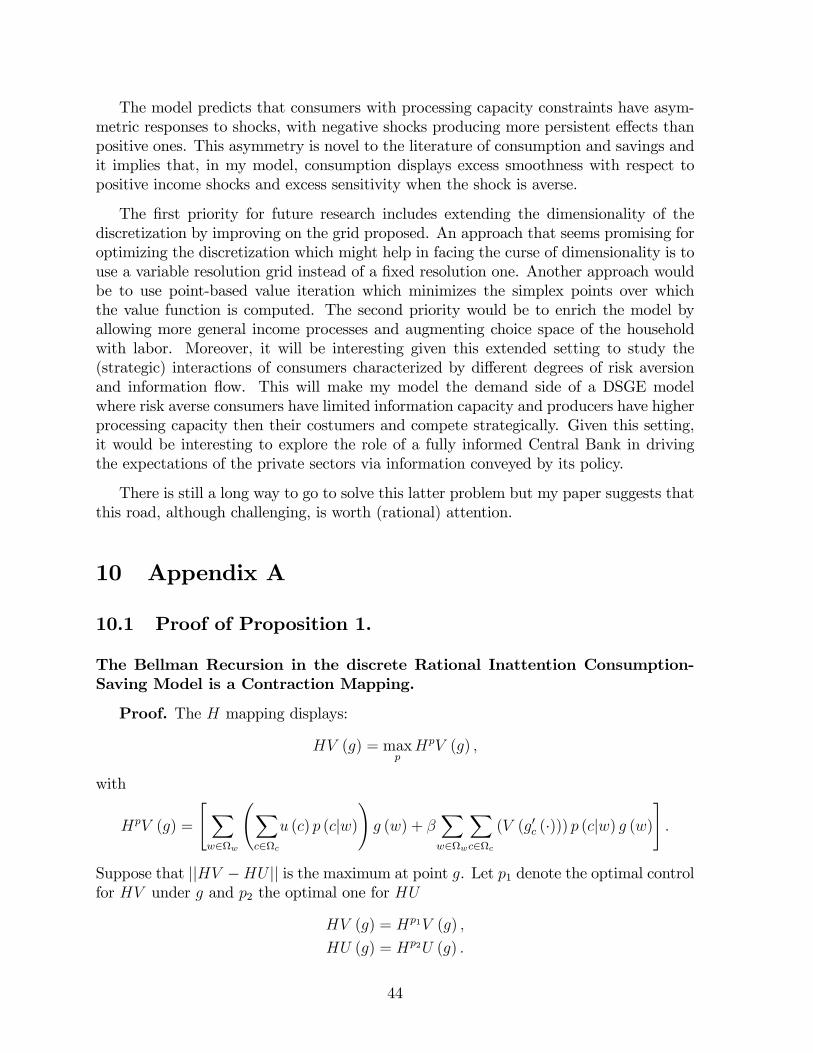
The model predicts that consumers with processing capacity constraints have asym-metric responses to shocks, with negative shocks producing more persistent e¤ects thanpositive ones. This asymmetry is novel to the literature of consumption and savings andit implies that, in my model, consumption displays excess smoothness with respect topositive income shocks and excess sensitivity when the shock is averse.

The �rst priority for future research includes extending the dimensionality of thediscretization by improving on the grid proposed. An approach that seems promising foroptimizing the discretization which might help in facing the curse of dimensionality is touse a variable resolution grid instead of a �xed resolution one. Another approach wouldbe to use point-based value iteration which minimizes the simplex points over whichthe value function is computed. The second priority would be to enrich the model byallowing more general income processes and augmenting choice space of the householdwith labor. Moreover, it will be interesting given this extended setting to study the(strategic) interactions of consumers characterized by di¤erent degrees of risk aversionand information �ow. This will make my model the demand side of a DSGE modelwhere risk averse consumers have limited information capacity and producers have higherprocessing capacity then their costumers and compete strategically. Given this setting,it would be interesting to explore the role of a fully informed Central Bank in drivingthe expectations of the private sectors via information conveyed by its policy.

There is still a long way to go to solve this latter problem but my paper suggests thatthis road, although challenging, is worth (rational) attention.

10 Appendix A

10.1 Proof of Proposition 1.

The Bellman Recursion in the discrete Rational Inattention Consumption-Saving Model is a Contraction Mapping.

Proof. The H mapping displays:

HV (g) = maxpHpV (g) ;

with

HpV (g) =

"Xw2w

Xc2c

u (c) p (cjw)!g (w) + �

Xw2w

Xc2c

(V (g0c (�))) p (cjw) g (w)#:

Suppose that jjHV �HU jj is the maximum at point g. Let p1 denote the optimal controlfor HV under g and p2 the optimal one for HU

HV (g) = Hp1V (g) ;

HU (g) = Hp2U (g) :

44

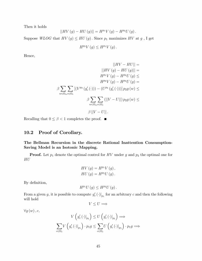
Then it holdsjjHV (g)�HU (g)jj = Hp1V (g)�Hp2U (g) :

Suppose WLOG that HV (g) � HU (g) : Since p1 maximizes HV at g , I get

Hp2V (g) � Hp1V (g) :

Hence,

jjHV �HU jj =jjHV (g)�HU (g)jj =Hp1V (g)�Hp2U (g) �Hp2V (g)�Hp2U (g) =

�Xw2w

Xc2c

[(V p2 (g0c (�)))� (Up2 (g0c (�)))] p2g (w) �

�Xw2w

Xc2c

(jjV � U jj) p2g (w) �

� jjV � U jj :Recalling that 0 � � < 1 completes the proof.

10.2 Proof of Corollary.

The Bellman Recursion in the discrete Rational Inattention Consumption-Saving Model is an Isotonic Mapping.

Proof. Let p1 denote the optimal control for HV under g and p2 the optimal one forHU

HV (g) = Hp1V (g) ;

HU (g) = Hp2U (g) :

By de�nition,Hp1U (g) � Hp2U (g) :

From a given g, it is possible to compute g0c (�)jp1 for an arbitrary c and then the followingwill hold

V � U =)8g (w) ; c;

V�g0c (�)jp1

�� U

�g0c (�)jp1

�=)X

c2c

V�g0c (�)jp1

�� p1g �

Xc2c

U�g0c (�)jp1

�� p1g =)

45

Xw2w

Xc2c

u (c) p1

!g (w) + �

Xc2c

V�g0c (�)jp1

�� p1g

�Xw2w

Xc2c

u (c) p1

!=)

Hp1V (g) � Hp1U (g) =)Hp1V (g) � Hp2U (g) =)HV (g) � HU (g) =)

HV � HU:

Note that g was chosen arbitrarily and, from it, g0c (�)jp1 completes the argument that thevalue function is isotone.

10.3 Proof of Proposition 2.

The Optimal Value Function in the discrete Rational Inattention Consumption-Saving Model is Piecewise Linear and Convex (PCWL).

Proof. The proof is done via induction. I assume that all the operations are well-de�ned in their corresponding spaces. For planning horizon n = 0, I have only to takeinto account the immediate expected rewards and thus I have that:

V0 (g) = maxp2�

"Xw2w

Xc2c

u (c) p

!g (w)

#(30)

and therefore if I de�ne the vectors

��i0 (w)

i� Xc2c

u (c) p

!p2�

(31)

I have the desiredV0 (g) = max

f�i0(w)gi

�i0; g

�(32)

where h:; :i denotes the inner product h�i0; gi �Xw2w

�i0 (w) ; g (w).For the general case,

using equation (25):

Vn (g) = maxp2�

26664Xw2w

Xc2c

u (c) p (cjw)!g (w)+

+�Xw2w

Xc2c

(Vn�1 (g0c (�)c)) p (cjw) g (w)

37775 (33)

46

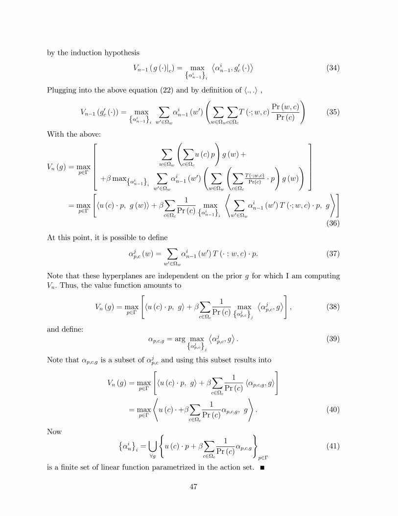
by the induction hypothesis

Vn�1 (g (�)jc) = maxf�in�1gi

�in�1; g

0c (�)�

(34)

Plugging into the above equation (22) and by de�nition of h:; :i ,

Vn�1 (g0c (�)) = max

f�in�1gi

Xw02w

�in�1 (w0)

Xw2w

Xc2c

T (�;w; c) Pr (w; c)Pr (c)

!(35)

With the above:

Vn (g) = maxp2�

266664Xw2w

Xc2c

u (c) p

!g (w)+

+�maxf�in�1giXw02w

�in�1 (w0)

Xw2w

Xc2c

T (�;w;c)Pr(c)

� p!g (w)

!377775

= maxp2�

"hu (c) � p; g (w)i+ �

Xc2c

1

Pr (c)maxf�in�1gi

* Xw02w

�in�1 (w0)T (�;w; c) � p; g

+#(36)

At this point, it is possible to de�ne

�jp;c (w) =Xw02w

�in�1 (w0)T (� : w; c) � p: (37)

Note that these hyperplanes are independent on the prior g for which I am computingVn: Thus, the value function amounts to

Vn (g) = maxp2�

"hu (c) � p; gi+ �

Xc2c

1

Pr (c)maxf�jp;cg

j

�jp;c; g

�#; (38)

and de�ne:�p;c;g = arg max

f�jp;cgj

�jp;c; g

�: (39)

Note that �p;c;g is a subset of �jp;c and using this subset results into

Vn (g) = maxp2�

"hu (c) � p; gi+ �

Xc2c

1

Pr (c)h�p;c;g; gi

#

= maxp2�

*u (c) �+�

Xc2c

1

Pr (c)�p;c;g; g

+: (40)

Now ��ini=[8g

(u (c) � p+ �

Xc2c

1

Pr (c)�p;c;g

)p2�

(41)

is a �nite set of linear function parametrized in the action set.

47

10.4 Proof of Proposition 3.

Proof. The �rst task is to prove that f�ingi sets are discrete for all n. The proof proceedsvia induction. Assuming CRRA utility and since the optimal policy belongs to �, it isstraightforward to see that through (31), the set of vectors f�i0gi,�

�i0i� Xw2w

Xc2c

c1�

1� p (cjw)

!g (w)

!p2�

is discrete. For the general case, observe that for discrete controls and assuming M =����jn�1��, the sets ��jp;c are discrete, for a given action p and consumption c, I can onlygenerate �jp;c�vectors. Now, �xing p it is possible to select one of theM �jp;c�vectors foreach one of the observed consumption c and, thus, f�jngi is a discrete set. The previousproposition, shows the value function to be convex. The piecewise-linear component ofthe properties comes from the fact that f�jngi set is of �nite cardinality. It follows thatVn is de�ned as a �nite set of linear functions.

11 Appendix B

11.1 Concavity of Mutual information in the Belief State.

For a given p (cjw),Mutual Information is concave in g (w)

Proof. Let Z be the binary random variable with P (Z = 0) = � and let W = W1 ifZ = 0 and W = W2 if Z = 1. Consider

I (W;Z;C) = I (W ;C) + I (Z;CjW )= I (W ;CjZ) + I (Z;C)

Condition on W , C and Z are independent, I (C;ZjW ) = 0: Thus,

I (W ;C) � I (W ;CjZ)= � (I (W ;CjZ = 0)) + (1� �) (I (W ;CjZ = 1))= � (I (W1;C)) + (1� �) (I (W2;C))

Q.E.D.

12 Appendix C

12.1 Optimality Conditions

Derivative with Respect to Controls In the main text, I state that the optimalcontrol amounts to :

48

@p� (ck1 ; wk2) :

�ku (c (�)) + ��kV (g0c (:)) = p� (ck1 ; wk2) (���ku

0 (c (�)) + ��kVp� (g0c (:))) (42)

which can be rewritten, opening up the operator �k as:

'�(ck1 ;ck2)= Pr (ck1 ; wk2)

0@ �(ck1 ;ck2 ;�) ln Pr (ck1 ; wk2)Pr (ck1)+ �

24@V 0�g0ck1

(�)�

@ Pr (ck1 ; wk2)�@V 0

�g0ck2

(�)�

@ Pr (ck1 ; wk2)

351Awhere

� '�(ck1 ;ck2)

� �hu (ck1 (�))� u (ck2 (�)) + �

�V�g0ck1

(�)�� V

�g0ck2

(�)��i

, and

� �(ck1 ;ck2 ;�)� �� [u0 (ck1 (�))� u0 (ck2 (�))] :

Note that by Chain rule@V 0

�g0ckj

(�)�

@ Pr(ckj ;wk2)=

@V 0�g0ckj

(�)�

@

�g0ckj

(�)� @

�g0ckj

(�)�

@ Pr(ckj ;wk2), for j = 1; 2: Plug (26) in

the second term of the above expression and evaluating pointwise the derivatives delivers

In cj = ck1 ;

=)@g

��jck1

�@ Pr(ck1 ;wk2)

=@

"1

p(ck1)

Pi

T(�;wi;ck1)Pr(wi;ck1)!#

@ Pr(ck1 ;wk2)=

1

p (ck1)

0BB@T (�;wk2 ; ck1)��P

i

T (�;wi; ck1) Pr (wi; ck1)�

p (ck1)

1CCADe�ne � �

'�

(ck1 ;ck2) �

(ck1 ;ck2)and �� � �

�

(ck1 ;ck2 ;�); and to get rid of cumbersome nota-

tion, let (k1; k2) ���;��; g0ck1

(�) ; g0ck2 (�) ;Pr (ck1 ; wk2) ;�: Then the �rst order

conditions result into

Pr (ck1 ; wk2) = � (k1; k2) Pr (ck1) (43)

where

� (k1; k2) � �1 (�;Pr (ck1 ; wk2))��2���; g0ck1

(�) ;Pr (ck1 ; wk2)���3���; g0ck2

(�) ;Pr (ck1 ; wk2)�

while

49

� �1 (�;Pr (ck1 ; wk2)) � e

0B@� 1

Pr(ck1 ;wk2)

1CA;

� �2���; g0ck1

(�) ;Pr (ck1 ; wk2)�� e

0BBB@��� @V�g0ck1

(�)�

@

�g0ck1

(�)� 1

p(ck1)

0BBB@T(�;wk2 ;ck1)�0@P

i

T(�;wi;ck1)Pr(wi;ck1)1A

p(ck1)

1CCCA1CCCA;

� �3 (k1; k2) � e

0BBB@�� @V�g0ck2

(�)�

@

�g0ck2

(�)� 1

p(ck2)

0BBB@T(�;wk2 ;ck2)�0@P

i

T(�;wi;ck1)Pr(wi;ck2)1A

p(ck2)

1CCCA1CCCA:

Derivative with Respect to States To derive the envelope condition with respectto a generic state g (wk) for k = 1; 2; 3, let me start by placing the restrictions on themarginal distribution of wealth in the main diagonal of the joint distribution Pr (c; w).The derivative then amounts to:

@ Pr t(cj ;wk)

@g(wk)=

@ Pr t(cj)

@g(wk)=

8<:1 f(j = k) \ (j 6= max l 2 c)g�1 fj = max l 2 cg0 o/whise

:

Let lmax denote the maximum indicator l belonging to c: Then the derivative of thestate g (wk) displays:

@V (g(wk))@g(wk)

a:s=�

u (ck (�)) + ��V�g0ck (�)

����u�clmax

(�)�+ �V

�g0clmax

(�)���

+

���log�Pr(ck;wk)p(ck)g(wk)

�u0 (ck (�)) Pr (ck; wk)� log

�Pr(clmax ;wk)p(clmax )g(wk)

�u0�clmax (�)

�Pr�clmax ; wk

��+

+�P

j

"@V

�g0ckj

(�)�

@

�g0ckj

(�)� @

�g0ckj

(�)�

@g(wk)

!Pr (cj; wk)

#:

Combining �rst order conditions and envelopes condition after some algebra amountto the result in (43).

13 Appendix D

13.1 Analytical Results for a three-point distribution

In this section I will specialize the optimality conditions derived above for a three pointdistribution. The goal is to fully characterize the solution for this particular case and

50

explore its insights.16

Let me assume the wealth to be a random variable that takes up values in w 2w � fw1; w2; w3g with distribution g (wi) = Pr (w = wi) described by:

W wl wm wh

g (wi) g1 g2 1� g1 � g2

The equation describing the evolution of the wealth is displayed by the budget constraint

wt+1 = R (wt � ct) + Yt

where I denote by Yt the exogenous stochastic income process earned by the householdand by R > 0 the (constant) interest rate on savings, (wt � ct). Like wealth, beforeprocessing information consumption, ct; is a random variable. It takes up a discretenumber of values in the event space c � fc1; c2; c3g. The joint distribution of wealthand consumption, Pr t (cj; wi), amounts to:

Pr t (cj; wi)

CnW w1 w2 w3

c1 x1 x2 x3c2 0 x4 x5c3 0 0 x6

where the zeros in the SW end of the matrix encodes the feasibility constraint wi (t) �cj (t) 8i 2 w; j 2 c and 8t � 0. The additional restrictions to the above matrix arethe ones commanded by the marginal on wealth. That is:

x1 = g1

x2 + x4 = g2

x3 + x5 + x6 = 1� g1 � g2

Without loss of generality, I place the marginal distribution of wealth in the main diagonalof Pr t (cj; wi) and I impose the restrictions above together with the condition that theresulting matrix describes a proper distribution. The joint distribution of wealth andconsumption amounts to:

Pr (cj; wi) :

CnW w1 w2 w3

c1 g1 p1 p2c2 0 g2 � p1 p3c3 0 0 1� (g1 + g2)� (p2 + p3)

(44)

16Three-point distribution is indeed a special case of the more general N points distribution since twoof the states in the event space w are absorbing states. This, in turn, sets to zero several dimensions ofthe problem and allows for a close form solution of the optimal policies. Although the solution for thisparticular case does not have a straightforward generalization, it provides useful insights on the optimalchoice for the joint probability distribution of wealth and consumption and its relation with the priordistribution of wealth -g (w)- and the utility of the consumer.

51

The resulting marginal distribution of consumption that endogenously depends on thechoices of pi�s, i = 1; 2; 3; displays:

Pr (C = cj) =

8<:c1 w.p g1 + p1 + p2c2 w.p g2 � p1 + p3c3 w.p 1� (g1 + g2)� (p2 + p3)

:

Once the consumer chooses pi�s and observes the realized consumption ct, he updatesthe marginal distribution of wealth. The latter, g0

��jcj�, is obtained combining the

joint distribution of wealth and consumption and the transition probability function. Informulae, the updated marginal on wealth amounts to:

g0��jcj�=Pi

T (�;wi; cj) Pr (wijcj) : (45)

The speci�cation of T (�;wi; cj) adopted in the analytical derivation of the discrete prob-ability distribution as well as in the numerical simulation can be explained as follows.The transition probability function is meant to approximate the expected value of nextperiod wealth:

EW 0 = R (wt � ct) + �Y : (46)

The approximation is necessary since (46) cannot hold exactly at the boundaries of thesupport of the wealth, w. In the above equation, R is the interest rates assumed to be agiven number while �Y is the mean of the stochastic income process, Yt. Suppose we have athree point distribution. AssumeWLOG that the values wi 2 w are equally spaced. Fora given (wi; cj) pair, the distribution of next period wealth is concentrated on three w0i val-ues closest to R (wi � cj)+ �Y , which will be denoted by !1; !2; !3 with respective proba-bilities �1; �2; �3. The mean of the distribution is ��1 (!2 � !1)+�3 (!3 � !2)+!2. Let �be the distance between the values of wi: Then the mean becomes �! � �� (�3 � �1)+!2.The variance of the distribution is then �2! � �2 (�3 � �1) � (�! � !2)

2. Since �2 is anexact function of �1 and �3, the equations for mean and variance of the process consti-tutes two equations in two unknowns. With the additional restriction that all the �i�sare positive and sum to one, it is not possible to guarantee the existence of a solution forR (wi � cj) + �Y close to the boundaries of the support of the distribution of wealth. Tomake sure that there is always a solution for �! 2 (min (w) + :5�;max (w)� :5�), andthe solution is continuous at points where �! =

(wi+wi+1)2

, one has to choose �2! = :25�2.

Euler Equations. Making use of the marginal distribution of wealth described aboveand making use of (45) together with the speci�cations of T (�;wi; cj) and Pr (wi; cj), Ican explicitly evaluate g0

��jcj�point-wise. To illustrate this point, using the numerical

values of T (�;wi; cj) above, the derivatives point-wise are as follows.

In cj = c1;

g0��jc1�=

1

(g1 + p1 + p2)(T (�;w1; c1) g1 + T (�;w2; c1) p1 + T (�;w3; c1) p2)

52

In cj = c2

g0��jc2�=

1

(g2 � p1 + p3)(T (�;w2; c2) (g2 � p1) + T (�;w3; c2) p3)

In cj = c3g0��jc3�= T (�;w3; c3)

Then, the �rst order conditions and envelope conditions amount to

@p1 : �u (c1)� u (c2) + �

�V 0 �g0c2 (�)�� V 0 �g0c2 (�)���

= p1

0@ � ([u0 (c1 � ��)� u0 (c2 � ��)]) ln�

p1(g1+p1+p2)

�+

+@V 0(g0c1 (�))@g0c1 (�)

@g0c1 (�)@p1

� @V 0(g0c2 (�))@g0c2 (�)

@g0c2 (�)@p1

1A

Note that@g0cj (�)@pj

= 0 for j 2 f1; 2; 3g.17 This result is not driven by the speci�ca-tion chosen for the transition function T (�;wi; cj) but it is a feature of the three pointdistribution. Indeed, since two of the three values of wealth are at the boundaries ofw, the absorbing states w1 and w3 place tight restrictions on the continuation valueV 0�g0cj (�)

�through the transition function and, as a result, the update for the marginal

g0cj (�) according to (45). That is, the marginal probability on wealth g0cj(�) in this case

tends to its ergodic value �gcj (�). It follows that V 0 ��gcj (�)� a:s:�! �V � ��gcj (�)� which is aconstant since the functional argument is. This is what makes the 3-point distributiontractable.

For the general case, the �rst order condition with respect to the �rst control amountsto:

@p1 : �u (c1 (�))� u (c2 (�)) + �

��V (�gc1 (�))� �V (�gc2 (�))

��= p1

�� ([u0 (c1 (�))� u0 (c2 (�))]) ln

�p1

(g1 + p1 + p2)

��(47)

17To see this, plug (45) in@g0cj

(�)@pj

for j 2 f1; 2g and evaluating pointwise the derivatives delivers@g0��jc1�:

1

(g1 + p1 + p2)2

24 0:81p2 � 0:15g1� (0:56p2 � 0:15g1)

�0:25p2

35 = 0@g0��jc2�:

p3

(g2 � p1 + p3)2

24 �0:150:150

35 = 0

53

Similarly, for the second control

@p2 : �u (c1 (�))� u (c3 (�)) + �

��V (�gc1 (�))� �V (�gc3 (�))

��= p2

�� ([u0 (c1 (�))� u0 (c3 (�))]) ln

�p2

(g1 + p1 + p2)

��(48)

And �nally:

@p3 : �u (c2 (�))� u (c3 (�)) + �

��V (�gc2 (�))� �V (�gc3 (�))

��= p3

�� (u0 (c2 (�))� u0 (c3 (�))) ln

�p3

(g2 � p1 + p3)

��(49)

Using the result that the value function converges to V � when the utility function be-longs to the family of absolute risk aversion (CARA), I assume the utility takes up thespeci�cation:

u (cj (�)) =

8><>:� e

� (cj(�))

for > 0

log (cj (�)) for lim !0

�� e

� (cj(�))

�where is the coe¢ cient of absolute risk aversion and j 2 c � fc1; c2; c3g. Moreover,by proposition 1, the value function is PCWL, that is:

�V��gcj (�)

�= arg max

f�0jgj

D�0j; �g

0cj(�)E

where��0jjare a set of vectors each of them generated for a particular observation of

previous values of consumption cj and h:; :i denotes the inner productD�0j; �g

0cj(�)E�X

w02w

�0j (w0)T (� : w; cj) � p (cjjw). To get a close form solution, I need to represent the

probability distribution of the prior. One of the possibilities is to use a particle basedrepresentation. The latter is performed by using N random samples, or particles, atpoints wi and with weights $i. The prior is then

gt (w) =NPi=1

$i~� (w � wi)

where ~� (w � wi) = Dirac (w � wi) is the Dirac delta function with center in zero. Aparticle-based representation can approximate arbitrary probability distributions (withan in�nite number of particles in the extreme case), it can accommodate nonlinear tran-sition models without the need of linearizing the model, and it allows several quantities of

54

interest to be computed e¢ ciently. In particular, the expected value in the belief updateequation becomes:

�g0��jcj�= Pr (cjj�)

NPi=1

$iT (�;wi; cj)

The central issue in the particle �lter approach is how to obtain a set of particles toapproximate �g0

��jcj�from the set of particles approximating g (w). The usual Sampling

Importance Re-sampling (SIR) approach (Dellaert et al., 1999; Isard and Blake, 1998)samples particles using the motion model T (�;wi; cj), then it assigns a new weights inorder to make all particles weights equal. The trouble with the SIR approach is that itrequires many particles to converge when the likelihood Pr (cjj�) is too peaked or whenthere is a small overlap between prior and posterior likelihood. he main problem withSIR is that it requires many particles to converge when the likelihood is too peaked orwhen there is only a small overlap between the prior and the likelihood. In the auxiliaryparticle �lter, the sampling problem is address by inserting the likelihood inside themixture

�g0��jcj�/

NXi=1

$i Pr (cjj�)T (�;wi; cj) :

The state (�) used to de�ne the likelihood Pr (cjj�) is not observed when the particles areresampled and this calls for the following approximation

�g0��jcj�/

NXi=1

$i Pr�cjj�i!

�T (�;wi; cj)

with �i! any likely value associated with the ith component of the transition densityT (�;wi; cj),

e.g., its mean. In this case, we have that �i! = wi + �(cj) : Then, �g0��jcj�can be re-

garded as a mixture of N transition components T (�;wi; cj) with weights $i Pr (cjj�i!) :Therefore, sampling a new particle w0j to approximate �g

0��jcj�can be carried out by

selecting one of the N components, say im, with probability $i � Pr (cjj�i!) and thensampling w0i from the corresponding component T (�;wim ; cj) : Sampling is performed inthe intersection of the prior and the likelihood and, consequently, particles with largerprior and larger likelihood (even if this likelihood is small in absolute value) are morelikely to be used. After the set of states for the new particles is obtained using the aboveprocedure, it is necessary to de�ne the weights. This is done using

$0m /

Pr (cjjw0m)Pr (cjj�im! )

:

Using the sample-based belief representation the averaging operator h:; :i can be com-

55

puted in close form as:

h�; �g0i =Xw2w

"Xk

$k� (wjwk;�k)#"X

l

$0l~� (w � wl)

#

=Xk

$k

Xw2w

� (wjwk;�k)

"Xl

$l~� (w � wl)

#!=Xk

$k

Xl

$l� (wljwk;�k)

=Xk;l

$k$l� (wljwk;�k) :

where � (:) is the distribution of the r.v. W 0 that use the speci�cation of the transitionfunction above, i.e., mean �! � �� (�3 � �1) + !2 and variance �2! � �2 (�3 � �1) �(�! � !2)

2 with � the (constant) distance between the values of wi.

Representing priors in this fashion allows an explicit evaluation of the di¤erences in thevalue functions in the �rst order conditions, since V 0

��g0cj (�)

�= argmaxf�0jgj

D�0j; �g

0cj(�)E=X

k;l

~$0k ~$

0l� (wljwk;�k), where ~$0

k ��Pr(cj jw0k)Pr(cj j�k!)

�; ~$0

l ��Pr(cj jw0l)Pr(cj j�l!)

�: Since the result of

the argmax is just one of the member of the set��0jjand all the elements involved in

the de�nition of �0j function in �(p) are a �nite set of linear function parametrized in theaction set, so is the �nal result.

Let a prime" 0 " denote the variables led one period ahead, algebraic manipulationdelivers the following optimal control functions:

p�1 (~g; �) =g1 ( 1 � ���1)

�g1 (LambertW (�1)x12 � LambertW (�11)x11) + 2g1 ( 1 � ��v1); (50)

p�2 (~g; �) =g1 ( 2 � ���2)

�g1 (LambertW (�2)x21 � LambertW (�2)x22) + 2 2g1 ( 2 � ���3); (51)

p�3 (~g) = 3 � ��v3

�x3 LambertW (�3)(52)

where

� 1 ��e� (c2���)e� (c1���)

�; 2 �

�e� (c3���)e� (c1���)

�; 3 �

�e� (c3���)e� (c2���)

�;

� �1 � g2 ( 03) + (g2 � g1) (

02 � 03) ;

56

� �2 � g2 ( 01) + (g2 � g1) (

01 � 02) ;

� �3 � (1� g2 � g1) ( 02) + (g2 � g1) (

03 � 01)

� �1 �( 1���v1) 1�g1(e (c2�c1))

; ; x11 � e� (c1���); x12 � e� (c2���);

� �21 �( 2���v2) 2�g1(e (c3�c1))

; x21 � e� (c1���); x22 � e� (c3���) and

� �3 � 3���v3

�g2(e (c3�c2)); x3 � e (c3�c2):

and LambertW (:) is the LambertW function that satis�es LambertW (x) eLambertW(x) =x18. The argument of the LambertW is always positive for the �rst order conditionsderived, implying that for each of the optimal policies the function returns a real solu-tion amongst other complex roots, which is unique and positive. Since @ LambertW(x)

@x=

LambertW(x)x(1+LambertW(x))

it is possible to calculate the derivatives of the above expression withrespect to f�; g1; g2g. However, the sign of the derivatives with respect to those variablesis indeterminate. The rational behind this result is quite simple. Consider the jointprobability distribution Pr (ci; wj) . The overall e¤ect of an increase in this probabil-ity results from the interplay of several factors. In general, if � is low -or, equivalently,the capacity of the channel, ��, in (21) is high-, a risk averse consumer will try to re-duce the o¤ diagonal term of the joint as much as possible. That is, he would setp1 = Pr (c1; w2) ; p2 = Pr (c1; w3) and p3 = Pr (c3; w2) as low as its capacity allows himto sharpen his knowledge of the state. On the opposite extreme, for very high value ofthe cost associated to information processing, �, p1 and p2 will be higher, the higher theprior g1 = g (w1) with respect to g2 = g (w2) and g3 = g (w3). This is due to the factthat when the capacity of the channel is low -or, equivalently, the e¤ort of processinginformation is high-, the �rst order conditions indicate that it is optimal for the con-sumer to shift probabilities towards the higher belief state. The intuition is that whenit is costly to process information, the household cannot reduce the uncertainty abouthis wealth. If the individual is risk adverse as implied by the CRRA utility function, ineach period, he would rather specialize in the consumption associated to the higher prior

18Formally, the LambertW function is the inverse of the function f : C ! C given by f (x) � xex:Hence LambertW (x) is the complex function that satis�es

LambertW (x) eLambertW(x) = x

for all x 2 C:. In practice the de�nition of LambertW requires a branch cut, which is usually takenalong the negative real axis. LambertW (x) function is sometimes also called product log function.This function allows to solve the functional equation

g (x)g(x)

= x

given thatg (x) = eLambertW(ln(x)):

See Corless, Gonnet, Hare, Je rey and Knuth (1996).

57

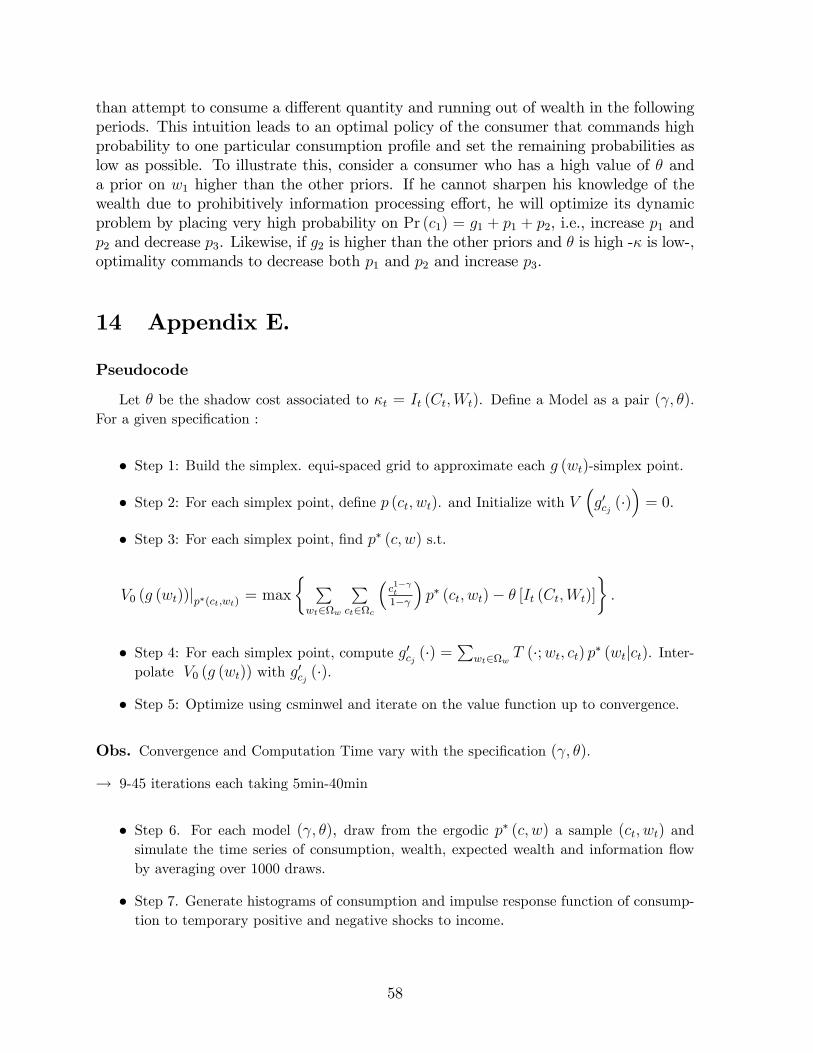
than attempt to consume a di¤erent quantity and running out of wealth in the followingperiods. This intuition leads to an optimal policy of the consumer that commands highprobability to one particular consumption pro�le and set the remaining probabilities aslow as possible. To illustrate this, consider a consumer who has a high value of � anda prior on w1 higher than the other priors. If he cannot sharpen his knowledge of thewealth due to prohibitively information processing e¤ort, he will optimize its dynamicproblem by placing very high probability on Pr (c1) = g1 + p1 + p2, i.e., increase p1 andp2 and decrease p3. Likewise, if g2 is higher than the other priors and � is high -� is low-,optimality commands to decrease both p1 and p2 and increase p3.

14 Appendix E.

Pseudocode

Let � be the shadow cost associated to �t = It (Ct;Wt). De�ne a Model as a pair ( ; �).For a given speci�cation :

� Step 1: Build the simplex. equi-spaced grid to approximate each g (wt)-simplex point.

� Step 2: For each simplex point, de�ne p (ct; wt). and Initialize with V�g0cj (�)

�= 0:

� Step 3: For each simplex point, �nd p� (c; w) s.t.

V0 (g (wt))jp�(ct;wt) = max� Pwt2w

Pct2c

�c1� t

1�

�p� (ct; wt)� � [It (Ct;Wt)]

�:

� Step 4: For each simplex point, compute g0cj (�) =P

wt2w T (�;wt; ct) p� (wtjct). Inter-

polate V0 (g (wt)) with g0cj (�).

� Step 5: Optimize using csminwel and iterate on the value function up to convergence.

Obs. Convergence and Computation Time vary with the speci�cation ( ; �).

! 9-45 iterations each taking 5min-40min

� Step 6. For each model ( ; �), draw from the ergodic p� (c; w) a sample (ct; wt) andsimulate the time series of consumption, wealth, expected wealth and information �owby averaging over 1000 draws.

� Step 7. Generate histograms of consumption and impulse response function of consump-tion to temporary positive and negative shocks to income.

58

References

[1] Allen, F., S. Morris and H. S. Shin, (2006), Beauty Contests, Bubbles and IteratedExpectations in Asset Markets Review of Financial Studies, forthcoming.

[2] Alvarez, F. and N. Stockey, (1998), Dynamic Programming with Homogeneous Func-tions, Journal of Economic Theory, 82, pp.167-189.

[3] Amato, J.S. Morris and H. S. Shin (2002), Communication and Monetary Policy,Oxford Review of Economic Policy 18, pp. 495-503.

[4] Ameriks, J., Andrew C. and J. Leahy (2003b) The Absent-Minded Consumer, un-published, New York University.

[5] Angeletos G.-M. and A. Pavan, (2004), Transparency of Information and Coordina-tion in Economies with Investment Complementarities, American Economic Review94 (2).

[6] Aoki, K. (2003), On the Optimal Monetary Policy Response to Noisy Indicators,Journal of Monetary Economics 50, pp. 501-523.

[7] Caballero, R. J. (1990), Expenditure on Durable Goods: a case for slow adjustment,The Quarterly Journal of Economics, Vol. 105, No. 3. pp. 727-743.

[8] Caballero, R. J. (1995), Near-rationality, Heterogeneity and Aggregate Consumption,Journal of Money, Credit and Banking, 27 (1), pp29-48.

[9] Campbell, J.Y. (1987), Does Savings Anticipate Declining Labor Income? An alter-native Test of the Permanent Income Hypothesis, Econometrica, 55, pp.1249-1273.

[10] Campbell, J.Y. and A. Deaton (1989), Why is Consumption so Smooth? Review ofEconomic Studies, 56, pp.357-374.

[11] Campbell, J.Y. and N. G. Mankiw (1989), Consumption, Income and Interest Rates:Reinterpreting the Time Series Evidence, NBER Macroeconomic Annual 4, pp.185-216.

[12] Campbell, J.Y. and N. G. Mankiw (1989), Permanent Income, Current Income andConsumption, Journal of Business and Economic Statistics, 8 (3), pp.265-279.

[13] Carroll, C. D. (2003) Macroeconomic Expectations of Households and ProfessionalForecasters, Quarterly Journal of Economics, 118 (1), pp. 269-298.

[14] Cochrane, J.H. (1989), The Sensitivity of Tests of the Intertemporal Allocationof Consumption to Near-Rational Alternatives, American Economic Review, 90,pp.319-337.

[15] Cover, T.M. and J. A. Thomas, Elements of Information Theory, John Wiley &Sons, Inc., 1991

59

[16] Deaton, A. (1987), Life-Cycle Models of Consumption: is the evidence consistentwith the Theory? in Advances in Econometrics, Fifth World Congress, vol.2, ed.Truman Bewley, Cambridge, Cambridge University Press.

[17] Deaton, A. (1992), Understanding Consumption, Oxford, Oxford University Press.

[18] Dynan, Karen (2000), Habit Formation in Consumer Preferences: Evidence fromPanel Data, American Economic Review, 90, pp. 391-406.

[19] Flavin, M. A. (1981), The Adjustment of Consumption to Changing Expectationsabout Future Income, Journal of Political Economy, 89, pp. 974-1009.

[20] Friedman, M. (1957), A Theory of the Consumption Function, Princeton, PrincetonUniversity Press.

[21] Goodfriend, Marvin (1992), Information-Aggregation Bias, American Economic Re-view, 82, pp. 508-519.

[22] Gourinchas, P-O, and J.A. Parker (2002), Consumption over the Life-Cycle, Econo-metrica, vol. 70 (1), pp.47-89.

[23] Hall, R. (1978), Stochastic Implications of the Life Cycle-Permanent Income Hy-pothesis: Theory and Evidence, Journal of Political Economy, 86, pp.971-987.

[24] Hellwig, C. (2004), Heterogeneous Information and the Bene�ts of Transparency,Discussion paper, UCLA.

[25] Hellwig, C. and L. Veldkamp, (2006) Knowing What Others Know: CoordinationMotives in Information Acquisition, NYU, mimeo.

[26] Kim, J., Kim, S., Schaumburg, E. and C. Sims (2005). Calculating and Using SecondOrder Accurate Solutions of Discrete Time Dynamic Equilibrium Models. mimeo.

[27] Lorenzoni, G. (2006), Demand Shocks and Monetary Policy, MIT, mimeo.

[28] Lucas, R. E., J. (1973), Some International Evidence on Output-In�ation Tradeo¤s,American Economic Review, 63(3), 326�334.

[29] Luo, Y. (2007), Consumption Dynamics, Asset Pricing, and Welfare E¤ects underInformation Processing Constraints, forthcoming in Review of Dynamics.

[30] Lusardi, A.(1999), Information, Expectations, and Savings, in Behavioral Di-mensions of Retirement Economics, ed. Henry Aaron, Brookings InstitutionPress/Russell Sage Foundation, New York, pp. 81-115.

[31] Lusardi, A. (2003), Planning and Savings for Retirement, Dartmouth College, un-published.

[32] MacKay, David J. C (2003). Information Theory, Inference, and Learning Algo-rithms, Cambridge University Press, 2003

60

[33] Macrowiack, B., and M. Wiederholt (2007), Optimal Sticky Prices under RationalInattention, Discussion paper, Northwestern/ ECB mimeo.

[34] Mankiw, N.G. and R. Reis (2002), Sticky information versus sticky prices: A pro-posal to replace the New Keynesian Phillips curve, Quarterly Journal of Economics117, 1295�1328.

[35] Mankiw, N. G., Reis, R. and J. Wolfers (2004) Disagreement in In�ation Expecta-tions, NBER Macroeconomics Annual 2003, vol. 18, pp. 209-147.

[36] Mondria, J. (2006), Financial Contagion and Attention Allocation, Working paper,University of Toronto.

[37] Morris, S., and H. S. Shin (2002), The Social Value of Public Information, AmericanEconomic Review, 92, 1521�1534.

[38] Moscarini, G. (2004), Limited Information Capacity as a Source of Inertia, Journalof Economic Dynamics and Control, pp. 2003�2035.

[39] Mullainathan, S. (2002), A Memory-Based Model of Bounded Rationality, QuarterlyJournal of Economics, 117 (3), pp. 735-774.

[40] Orphanides, A. (2003),Monetary Policy Evaluation with Noisy Information, Journalof Monetary Economics 50 (3), pp. 605-631.

[41] Parker, J. (1999) The Reaction of Household Consumption to Predictable Changesin Social Security Taxes, American Economic Review, 89 (4), pp. 959-973.

[42] Peng, L. (2005), Learning with Information Capacity Constraints, Journal of Finan-cial and Quantitative Analysis, 40(2), 307�329.

[43] Peng, L., and W. Xiong (2005), Investor Attention, Overcon�dence and CategoryLearning, Discussion paper, Princeton University.

[44] Puterman, M.L. (1994), Markov Decision Processes: Discrete Stochastic DynamicProgramming, Wiley Series in Probability and Mathematical Statistics, John Wileyand Sons, Inc.

[45] Reis, R. A. (2006) Inattentive Consumers, Journal of Monetary Economics, 53 (8),1761-1800.

[46] Schmitt-Grohè, S. and M. Uribe(2004). Solving Dynamic General Equilibrium Mod-els Using a Second-Order Approximation to the Policy Function. Journal of Eco-nomic Dynamics and Control 28, pp.755-75

[47] Sims, C. A. (1998), Stickiness, Carnegie-rochester Conference Series On Public Pol-icy, 49(1), 317�356.

[48] Sims, C. A. (2003), Implications of Rational Inattention, Journal of Monetary Eco-nomics, 50(3), 665�690.

61

[49] Sims, C. A.(2005), Rational Inattention: a Research Agenda, Princeton Universitymimeo.

[50] Van Nieuwerburgh, S., and L. Veldkamp (2004a), Information Acquisition and Port-folio Under-Diversication, Discussion paper, Stern School of Business, NYU.

[51] Stokey, N. L. and R. E. Lucas Jr., with Edward C. Prescott (1989) Recursive Methodsin Economic Dynamics, Cambridge, Harvard University Press.

[52] Van Nieuwerburgh, S., and L. Veldkamp (2004b), Information Immobility and theHome Bias Puzzle, Discussion paper, Stern School of Business, NYU.

[53] Van Nieuwerburgh, S., and L. Veldkamp, 2006, Learning Asymmetries in Real Busi-ness Cycles, Journal of Monetary Economics 53 (4), pp.753-772.

[54] Wilson, Andrea (2003) �Bounded Memory and Biases in Information Processing,�unpublished, Princeton University.

[55] Woodford, M. (2002), Imperfect Common Knowledge and the E¤ects of MonetaryPolicy, in P. Aghion, R. Frydman, J. Stiglitz, and M. Woodford, eds., Knowledge,Information, and Expectations in Modern Macroeconomics: In Honor of Edmund S.Phelps, Princeton: Princeton University Press.

[56] Woodford, M. (2003), Interest and Prices, Princeton. Princeton University Press

[57] Zeldes, S. (1989) Optimal Consumption with Stochastic Income: Deviations fromCertainty Equivalence, Quarterly Journal of Economics, May 1989, 275-98..

62

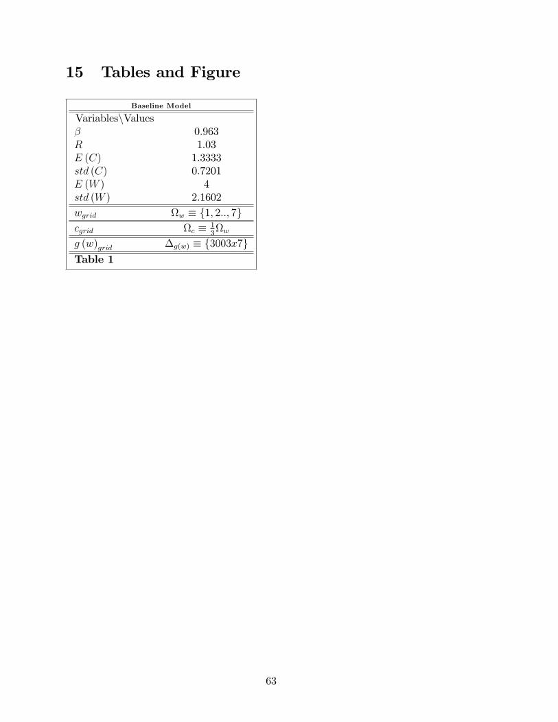
15 Tables and Figure

Baseline Model

VariablesnValues� 0.963R 1.03E (C) 1.3333std (C) 0.7201E (W ) 4std (W ) 2.1602wgrid w � f1; 2::; 7gcgrid c � 1

3w

g (w)grid �g(w) � f3003x7gTable 1

63

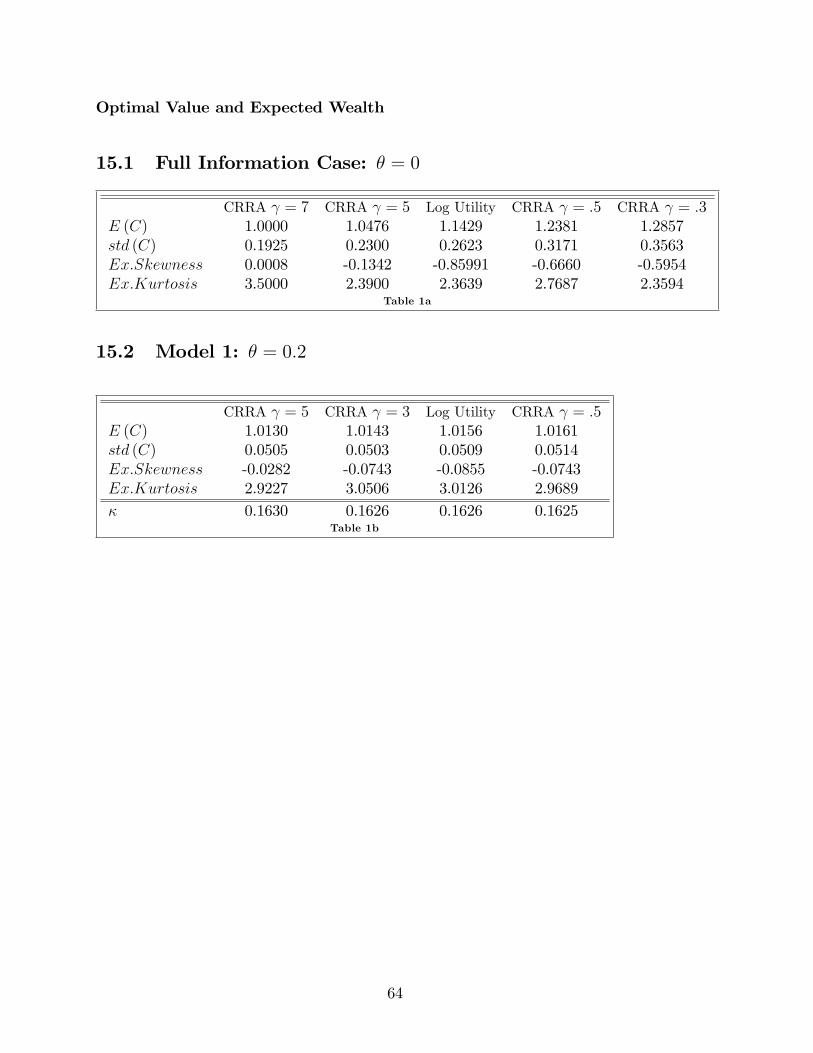
Optimal Value and Expected Wealth

15.1 Full Information Case: � = 0

CRRA = 7 CRRA = 5 Log Utility CRRA = :5 CRRA = :3E (C) 1.0000 1.0476 1.1429 1.2381 1.2857std (C) 0.1925 0.2300 0.2623 0.3171 0.3563Ex:Skewness 0.0008 -0.1342 -0.85991 -0.6660 -0.5954Ex:Kurtosis 3.5000 2.3900 2.3639 2.7687 2.3594

Table 1a

15.2 Model 1: � = 0:2

CRRA = 5 CRRA = 3 Log Utility CRRA = :5E (C) 1.0130 1.0143 1.0156 1.0161std (C) 0.0505 0.0503 0.0509 0.0514Ex:Skewness -0.0282 -0.0743 -0.0855 -0.0743Ex:Kurtosis 2.9227 3.0506 3.0126 2.9689� 0.1630 0.1626 0.1626 0.1625

Table 1b

64

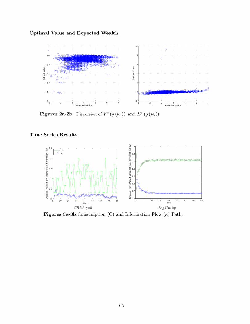
Optimal Value and Expected Wealth

1 2 3 4 5 6 7­5

­4

­3

­2

­1

0

1

Expected Wealth

Opt

imal

 Val

ue

1 2 3 4 5 6 7­2

0

2

4

6

8

10

Expected Wealth

Opt

imal

 Val

ue

Figures 2a-2b: Dispersion of V � (g (wi)) and E� (g (wi))

Time Series Results

0 10 20 30 40 50 60 70 800

0.5

1

1.5

2

2.5

time

Sim

ulat

ed T

ime 

Path

 of C

onsu

mpt

ion 

and 

Info

rmat

ion 

Flow C

κ

CRRA =5

0 10 20 30 40 50 60 70 800

0.2

0.4

0.6

0.8

1

1.2

1.4

time

Sim

ulat

ed T

ime 

Pat

h of

 Con

sum

ptio

n an

d In

form

atio

n Fl

ow

Log Utility

Figures 3a-3b:Consumption (C) and Information Flow (�) Path.

65

15.2.1 Histogram of Consumption

0.7 0.8 0.9 1 1.1 1.2 1.3 1.40

10

20

30

40

50

60

70clogc

γ05c

γ3c

γ5

Figures 4a: Consumption Path for several Utility Speci�cations.

66

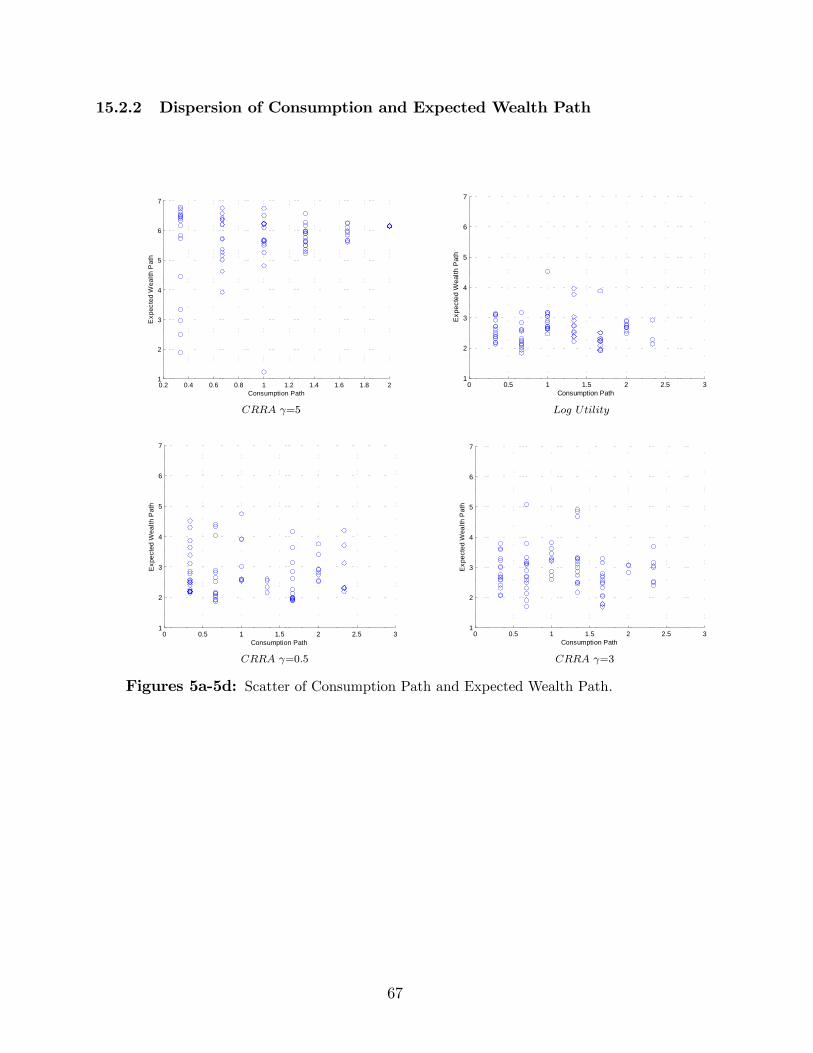
15.2.2 Dispersion of Consumption and Expected Wealth Path

0.2 0.4 0.6 0.8 1 1.2 1.4 1.6 1.8 21

2

3

4

5

6

7

Consumption Path

Exp

ecte

d W

ealth

 Pat

h

CRRA =5

0 0.5 1 1.5 2 2.5 31

2

3

4

5

6

7

Consumption Path

Exp

ecte

d W

ealth

 Pat

h

Log Utility

0 0.5 1 1.5 2 2.5 31

2

3

4

5

6

7

Consumption Path

Exp

ecte

d W

ealth

 Pat

h

CRRA =0:5

0 0.5 1 1.5 2 2.5 31

2

3

4

5

6

7

Consumption Path

Exp

ecte

d W

ealth

 Pat

h

CRRA =3

Figures 5a-5d: Scatter of Consumption Path and Expected Wealth Path:

67

15.3 Model 2 � = 1

CRRA = 7 CRRA = 5 CRRA = 3 Log Utility CRRA = :3E (C) 1.0213 1.0156 1.0148 1.0143 1.0138std (C) 0.0515 0.0503 0.0513 0.0513 0.0513Ex:Skewness -0.1086 -0.0855 0.0183 0.0254 0.0109Ex:Kurtosis 3.1786 3.0126 2.8750 2.9549 2.9337� 0.1729 0.1625 0.1622 0.1619 0.1612

Table 1c

Time Series Results

0 10 20 30 40 50 60 70 800

0.5

1

1.5

2

2.5

time

Sim

ulat

ed T

ime 

Path

 of C

onsu

mpt

ion 

and 

Info

rmat

ion 

Flow

Cκ

CRRA =5

0 10 20 30 40 50 60 70 800

0.5

1

1.5

2

2.5

time

Sim

ulat

ed T

ime 

Path

 of C

onsu

mpt

ion 

and 

Info

rmat

ion 

Flow

Cκ

Log Utility

0 10 20 30 40 50 60 70 800

0.5

1

1.5

2

2.5

time

Sim

ulat

ed T

ime 

Pat

h of

 Con

sum

ptio

n an

d In

form

atio

n Fl

ow

Cκ

CRRA =3

0 10 20 30 40 50 60 70 800

0.5

1

1.5

2

2.5

time

Sim

ulat

ed T

ime 

Path

 of C

onsu

mpt

ion 

and 

Info

rmat

ion 

Flow C

κ

CRRA =0:3

Figures 3c-3d:Consumption (C) and Information Flow (�) Path.

68

15.3.1 Dispersion of Consumption and Expected Wealth Paths

0.2 0.4 0.6 0.8 1 1.2 1.4 1.6 1.8 21

2

3

4

5

6

7

Consumption Path

Expe

cted

 Wea

lth P

ath

CRRA =0:3

0 0.5 1 1.5 2 2.51

2

3

4

5

6

7

Consumption Path

Expe

cted

 Wea

lth P

ath

Log Utility

0.2 0.4 0.6 0.8 1 1.2 1.4 1.6 1.8 21

2

3

4

5

6

7

Consumption Path

Expe

cted

 Wea

lth P

ath

CRRA =3

0.2 0.4 0.6 0.8 1 1.2 1.4 1.6 1.8 21

2

3

4

5

6

7

Consumption Path

Expe

cted

 Wea

lth P

ath

CRRA =7

Figures 5e-5h: Scatter of Consumption Path and Expected Wealth Path:

69

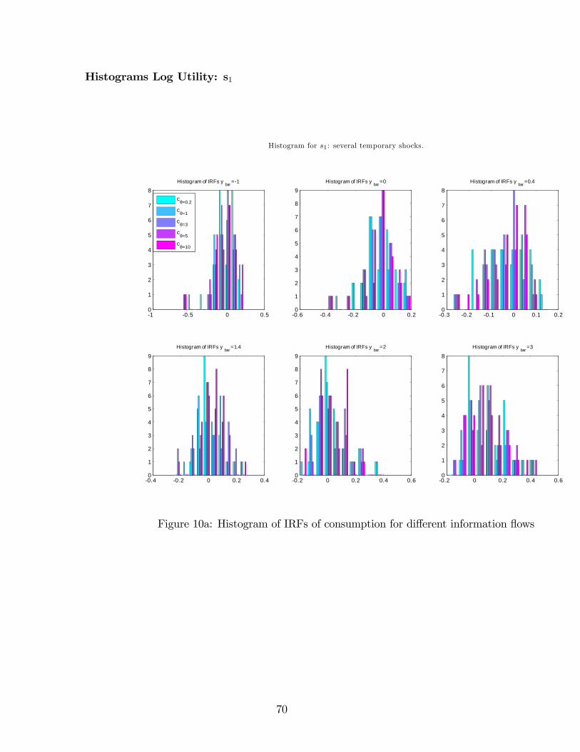
Histograms Log Utility: s1

Histogram for s1: several temporary shocks.

­1 ­0.5 0 0.50

1

2

3

4

5

6

7

8Histogram of IRFs y bar =­1

cθ=0.2

cθ=1

cθ=3

cθ=5

cθ=10

­0.6 ­0.4 ­0.2 0 0.20

1

2

3

4

5

6

7

8

9Histogram of IRFs y bar =0

­0.3 ­0.2 ­0.1 0 0.1 0.20

1

2

3

4

5

6

7

8Histogram of IRFs y bar =0.4

­0.4 ­0.2 0 0.2 0.40

1

2

3

4

5

6

7

8

9Histogram of IRFs y

bar=1.4

­0.2 0 0.2 0.4 0.60

1

2

3

4

5

6

7

8

9Histogram of IRFs y

bar=2

­0.2 0 0.2 0.4 0.60

1

2

3

4

5

6

7

8Histogram of IRFs y

bar=3

Figure 10a: Histogram of IRFs of consumption for di¤erent information �ows

70

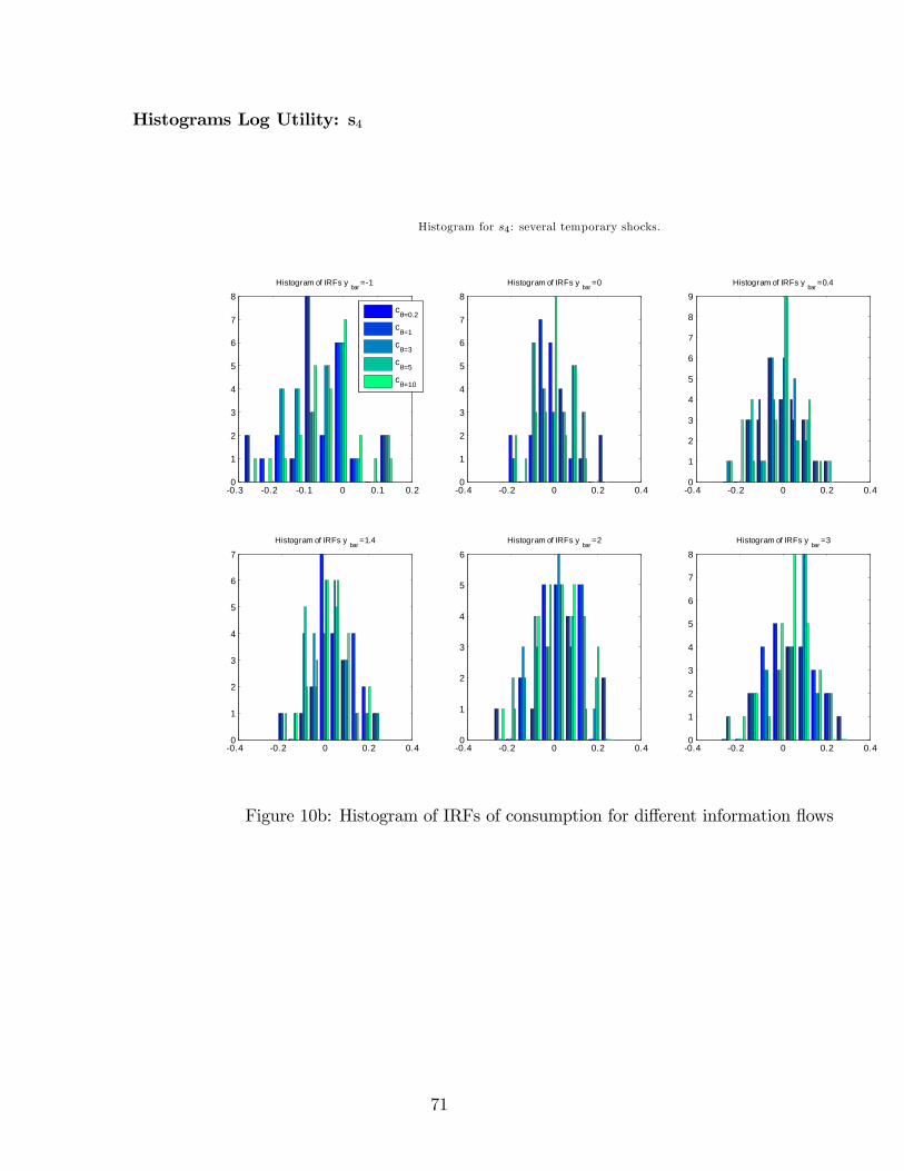
Histograms Log Utility: s4

Histogram for s4: several temporary shocks.

­0.3 ­0.2 ­0.1 0 0.1 0.20

1

2

3

4

5

6

7

8Histogram of IRFs y bar =­1

cθ=0.2

cθ=1

cθ=3

cθ=5

cθ=10

­0.4 ­0.2 0 0.2 0.40

1

2

3

4

5

6

7

8Histogram of IRFs y bar =0

­0.4 ­0.2 0 0.2 0.40

1

2

3

4

5

6

7

8

9Histogram of IRFs y bar =0.4

­0.4 ­0.2 0 0.2 0.40

1

2

3

4

5

6

7Histogram of IRFs y

bar=1.4

­0.4 ­0.2 0 0.2 0.40

1

2

3

4

5

6Histogram of IRFs y

bar=2

­0.4 ­0.2 0 0.2 0.40

1

2

3

4

5

6

7

8Histogram of IRFs y

bar=3

Figure 10b: Histogram of IRFs of consumption for di¤erent information �ows

71

Impulse Response Functions

0 5 10 15 20 250.2

0.25

0.3

0.35

0.4

0.45

0.5

0.55

0.6

time

IRF 

cons

umpt

ion

IRF, Log Utility

θ=1θ=0.2

Figure 11a

0 5 10 15 20 250.2

0.25

0.3

0.35

0.4

0.45

0.5

0.55

0.6

0.65

time

IRF 

cons

umpt

ion

IRF, γ=5

θ=0.2θ=2

Figure 4a

72