Finance and Economics Discussion SeriesDivisions of Research & Statistics and Monetary Affairs

Federal Reserve Board, Washington, D.C.

The Rigidity of Choice. Lifecycle savings withinformation-processing limits

Antonella Tutino

2008-62

NOTE: Staff working papers in the Finance and Economics Discussion Series (FEDS) are preliminarymaterials circulated to stimulate discussion and critical comment. The analysis and conclusions set forthare those of the authors and do not indicate concurrence by other members of the research staff or theBoard of Governors. References in publications to the Finance and Economics Discussion Series (other thanacknowledgement) should be cleared with the author(s) to protect the tentative character of these papers.

The Rigidity of Choice.Lifecycle savings with information-processing limits

Antonella Tutino�

First version: November 2007 ; This version: October 2008

Abstract

This paper studies the implications of information-processing limits on the con-sumption and savings behavior of households through time. It presents a dynamicmodel in which consumers rationally choose the size and scope of the informationthey want to process concerning their �nancial possibilities, constrained by a Shan-non channel. The model predicts that people with higher degrees of risk aversionrationally choose more information. This happens for precautionary reasons since,with �nite processing rate, risk averse consumers prefer to be well informed abouttheir �nancial possibilities before implementing a consumption plan. Moreover,numerical results show that consumers with processing capacity constraints haveasymmetric responses to shocks, with negative shocks producing more persistente¤ects than positive ones. This asymmetry results in more savings. I show that thepredictions of the model can be e¤ectively used to study the impact of tax reformson consumers spending.

�COMMENTS WELCOME. E-mail: Antonella.Tutino@frb.gov. I am deeply indebted to ChrisSims whose countless suggestions, shaping in�uence and guidance were essential to improve the qualityof this paper. I thank Ricardo Reis for valuable advice, enduring and enthusiastic support. I amgrateful to Per Krusell for his insightful advice and stimulating discussions. I would also like to thankMike Kiley, Nobu Kiyotaki, Angelo Mele, Philippe-Emanuel Petalas, John M. Roberts, Charles Roddie,Sam Schulhofer-Wohl, Tommaso Treu, Mark Watson and Mirko Wiederholt. Finally I thank numerousseminar participants for many helpful comments and discussions. Any remaning errors are my own. Theviews in this paper are solely the responsibility of the author and should not be interpreted as re�ectingthe views of the Federal Reserve Board or any other person associated with the Federal Reserve System.

1

Information is, we must steadily remember, a measure of one�s freedom ofchoice in selecting a message. The greater this freedom of choice, and hencethe greater the information, the greater is the uncertainty that the message ac-tually selected is some particular one. Thus greater freedom of choice, greateruncertainty, greater information go hand in hand. (Claude Shannon, sic.)

1 Introduction

Every day people face an overwhelming amount of data. Every day, though, peopleuse these for their decisions. In selecting useful information, people face a trade o¤between reacting quickly and precisely to news about their �nancial possibilities and notspending time crunching numbers to �gure out their exact net worth. To match thesefacts, macroeconomists have adopted a number of modelling strategies able to injectinertia within the rational expectation framework. These devices, such as the costlyacquisition and di¤usion of information, largely rely on ad-hoc technology to generatesmooth and delayed responses of consumption to a shock to income consistent withobserved data. Contrary to this approach, this paper proposes a way to relate inertialbehavior in consumption and savings based on people�s preferences.

To this end, the paper o¤ers a micro-founded explanation on the nature of inertia inconsumption and savings. Following Rational Inattention (Sims, 2003, 2006), I modelthe limits of people to process information at an in�nite rate by using Shannon channels.

Under this information processing constraint, individuals choose a signal that con-veys information about their �nancial possibilities. The signal can provide any kind ofinformation as long as its overall content is within the channel�s capacity. Consumersbase their expectations of the economic conditions on the signal and decide how muchto consume. Thus, in my framework, the delayed and smoothed responses of savings tochanges in wealth are the result of a slow information �ow due to processing constraints.Combining the standard utility maximization framework subject to a budget constraintwith information processing limits leads to a departure from rational expectations. Mypaper shows how to model this formally in an intertemporal setting. In particular, Iassume that people do not know the exact value of their wealth but have an idea of theirnet worth. A way of thinking about this hypothesis is that people do not know exactlyof what the dollar value of their paycheck (nominal) corresponds to in terms of cups ofco¤ee (real), assuming that this is what they care about. People process information tosharpen their knowledge of how much consumption their wealth can purchase. I modelinitial uncertainty as a probability distribution over the possible realizations of wealth.In such a framework, it is possible to study how choices of information play out withpeople�s preferences when they decide on consumption throughout their life time.

The challenge of this model and, more generally, of models of rational inattention isdealing with the in�nite dimensional state space implied by having a prior as state. Forthis reason, the applications of rational inattention have been limited to either a linear

2

quadratic framework where Gaussian uncertainty has been considered (such as Sims 1998,2003, Luo 2007, Mackowiak and Wiederholt 2007, Mondria, 2006, Moscarini 2004) or atwo-period consumption-saving problem (Sims 2006) where the choice of optimal ex postuncertainty is analyzed for the case of log utility and two Constant Relative Risk Aversion(CRRA) utility speci�cations. The linear quadratic Gaussian (LQG) framework can beseen as a particular instance of rational inattention in which the optimal distributionchosen by the household turns out to be Gaussian. Gaussianity has two main advantages.First, it allows an explicit analytical solution for these models. One can show that theproblem can be solved in two steps. First, the information gathering scheme is foundand then, given the optimal information, the consumption pro�le. Second, it is easyto compare the results to a signal extraction problem. When looking at the behavior ofrational inattentive consumers, it is impossible to separate an exogenously given Gaussiannoise in the signal extraction model from an endogenous noise that is optimally chosento be Gaussian.

The tractability of rational inattention LQG models comes at the cost of restrictiveassumptions on preferences and the nature of the signal. Constraining uncertainty of theindividual to a quadratic loss / certainty equivalent setting does not take into accountthe possibility that the agent is very uncertain about his economic environment; ceterisparibus, more uncertainty generates second-order e¤ects of information that have �rstorder impact on individuals�decisions. In this sense, rational inattention LQG modelsare subject to the same limits as methods that use linear approximation of optimalityconditions to study stochastic dynamic models.1 With little uncertainty about the eco-nomic environment, linear approximations of the optimality conditions may provide afairly adequate description of the exact solution of the system. This fact suggests thatthe uncertainty at the individual level might actually be large, undermining the accuracyof both linearized and rational inattention LQG models. To assess the importance ofinformation choices for people�expectations, it is important to let consumers select theirinformation from a wider set of distributions that includes but it is not limited to theGaussian family.

The theoretical contribution of this paper is to provide the analytical and computa-tional tools necessary to apply information theory in a dynamic context with optimalchoice of ex-post uncertainty. I propose a methodology to handle the additional com-plexity without the LQG setting. I propose a discretization of the framework and deriveits theoretical properties. Then, I provide a computational strategy that is able to solvethe model.

Several predictions emerge from the model. Evaluating the unconditional momentsof the time series of consumption for a given degree of risk aversion, the �rst result of thepaper is that higher information costs are associated with more persistence and highervolatility. The seemingly paradoxical results of having sluggish and volatile consumption

1Since the work of Hall (1982), the assumption of certainty equivalence has also been questionedin the consumption savings literature with no information friction, starting from e.g. Blanchard andMankiw (1988).

3

at the same time can be reconciled if one considers that information-processing con-straints prevent the consumers to respond promptly to �uctuations in wealth. To makea concrete example, suppose a person starts o¤ with low wealth and initially choosesto consume a little. If he is risk averse, he may decide not to modify his consumptionpro�le until he acquires more information about his wealth. As he processes informationthrough time, he gets more and more data about his high value of wealth and changes hisconsumption when he is sure that he has saved enough to a¤ord a higher consumptionexpenditure. The more risk averse the consumer is, the longer he waits. The longerthe wait, the more wealth grows because of the accumulation of savings and currentincome. The combination of waiting while processing information and sharp changesonce information has been processed through time generates sluggishness and volatilityin consumption.

Second, by looking at the life-cycle pro�le of consumption I �nd that the behavior ofconsumption is smooth and persistent with several peaks along the simulated path. Thesepeaks in consumption occur later in life for people that have access to low information�ow. This e¤ect is stronger as risk aversion increases. The logic behind this result is thatrisk averse consumers react to uncertainty by processing more information on their lowvalues of wealth and keep their consumption low as a precaution until the uncertainty isdiminished. They accumulate more savings throughout early adult life than their in�nite-information-processing counterparts. They keep saving until the accumulation of wealthand information indicates that they can enjoy a high consumption pro�le.

This leads also to the �nding that individual consumption can have more than onehump along its path as wealth accumulates through time. The key point is that individ-uals can vary their information �ow during their life time. To see why, suppose that aperson receives signals that his wealth is low. In this case, he wants to pay attention tohis expenses and closely monitor the activity of his account. Once he makes sure that hehas saved enough, he may decide to spend less e¤ort monitoring his balance and enjoyconsumption. Decumulation of savings continues until he receives information that hehas emptied his checking account. This news call for his attention again, so he startssaving and monitor his balance more frequently than before. These results combined aresuggestive of a precautionary motive for savings driven by information processing limits.

Third, I �nd that consumers with processing capacity constraints have asymmetricresponses to income �uctuations, with negative shocks producing sharper and more per-sistent e¤ects than positive ones. This e¤ect is stronger as the degree of risk aversionincreases. Compared with a situation in which there are no information-processing limits,in a rational-inattention consumption-savings model, an adverse temporary income shockmakes consumers reduce their consumption for a longer period of time. This happensbecause risk-averse people who receive bad news about their �nances save right awayto hedge against the possibility of running out of wealth in the future. Once they haveenough savings and information, they gradually increase their consumption and smooththe remaining e¤ect of the shock over time. This result also points toward precautionarymotive due to information-processing limits.

4

Finally, I �nd that the predictions of the model can be used to address importantpolicy questions. In the context of �scal reforms of consumer spending, I show that, aswealth decreases, rationally inattentive consumers respond faster to a tax rebate thatincreases their income by 10%. For a given level of wealth, the lower the processingcapacity, the longer it takes for consumption to react to shocks to disposable income.These �ndings make intuitive sense. A tax rebate matters more for people with lowerincome and, as a result, tighter budgetary constraints than for wealthy people.2 Asa result, poorer people acknowledge and react faster to the positive income shocks. Bycontrast, wealthy people do not perceive the increase in disposable income as a signi�cantchange in their �nancial position. Thus, consumption for wealthy people does not changesigni�cantly, instead it adjusts slowly over time. Consider an individual that has wealthand in�nite processing capacities. The reaction of consumption to a temporary positiveincome shock would be to adjust immediately to a new higher value of consumption soto smooth out the e¤ect of the shock throughout time. With limited processing capacity,the individual smooths consumption slowly over time because the e¤ect of the increasein disposable income on wealth spread out slowly through time. These predictions are inline with the empircal evidence on tax rebate (e.g., Johnson, Parker, and Soules (2006)).

My results are observational distinct from the previous literature on consumption andinformation (e.g., Reis (2006)). The distinguishing feature of my model with respect toprevious works is its ability to generate endogenously asymmetric response of consump-tion to shocks.3 Finally, my paper contributes to the literature that models how peopleform endogenously expectations and react to the economy on the basis of their rationallychosen information.4

The paper is organized as follows. Section 2 lays out the theoretical basis of rationalinattention and informally introduces the model. Section 3 states the problem of theconsumers as a discrete stochastic dynamic programming problem, while Section 4 derivesthe properties of the Bellman function. Section 5 provides the numerical methodologyused to solve the model. Section 6 delivers its main results. By comparing the predictionsof the model on the preliminary evidence on tax rebates, I �nd that the model can be avalid instrument to address the impact of tax reforms on consumer spending. Section 7concludes.

2Another way of looking at it is that people with lower income are generally more liquidity constrained.This makes their marginal propensity to consume to a positive shock closer to one than the wealthierpeople.

3In particular, for a given degree of risk aversion and magnitude of a shock, the response of con-sumption to a negative shock is stronger on impact and more persistent than the one to a positiveshock.

4A necessarily non-exhaustive list of papers that address the issue of modeling consumers� expec-tations includes the absent-minded consumer model proposed by Ameriks, Caplin and Leahy (2003),together with Mullainathan (2002) and Wilson (2005), whose models feature agents with imperfect re-call. Mankiw and Reis (2002) develop a di¤erent model in which information disseminates slowly dueto infrequent update of information.

5

2 Foundations of Rational Inattention

Rational inattention (Sims 1988,5 1998, 2003, 2005, 2006) blends two main �elds: Infor-mation Theory and Economics. The �rst draws mainly on the work of Shannon (1948).The main contribution is to de�ne a measure of the choice involved in the selection ofthe message and the uncertainty regarding the outcome. The measure used is entropy.Details on this part are in Appendix F. Based on Shannon�s apparatus, the economiccontribution is that of using Shannon capacity as a technological constraint to captureindividuals�inability of processing information about the economy at in�nite rate. Giventhese limits, people reduce their uncertainty by selecting the focus of their attention. Theresulting behavior depends on the choices of what to observe of the environment oncethe information-processing frictions are acknowledged.

2.1 The Economics of Rational Inattention

Consider a person who wants to buy lunch. He doesn�t know his exact wealth but heknows that he has some cash and a credit card. Not recalling the expenses charged on thecredit card up to that point, he can go to the bank or simply check his wallet. Going tothe bank to �gure out his wealth for lunch is beyond his time and interest, so he decidesto check his wallet. He browses through it thinking about what he wants and what he cana¤ord to buy for lunch. Mapping dollar bills into his knowledge of prices from previousconsumption, he realizes he can only a¤ord a sandwich instead of his favorite sushi roll.Then, he uses the receipt to update his prior on the price of sandwiches, what he thinkshe has left in his wallet and, ultimately, his wealth. This updated knowledge will be usedfor his next purchase. Such a story can be directly mapped into a rational inattentionframework.

First, the person does not know his wealth, W , but he has a prior on it, p (W ).Before processing any information, his uncertainty about wealth is the entropy of hisprior, H (W ) � �E[log2(p(W ))], where E [:] denotes the expectation operator.6 Beforeprocessing any information, lunch too is a random variable, C, ranging from sandwichesto sushi. To reduce entropy, he can choose whether to have a detailed report from thebank or to look at his wallet. The two options di¤er in amount of information and e¤ortin processing their content. The choice of the option (signal) together with consumptionresult in a joint probability p (c; w). Both dollars in the wallet and knowledge of prices ofsandwiches and sushi contribute to the reduction of uncertainty in wealth of an amountequal toH (W jC) = �

Rp (w; c) log2 p (wjc) dcdw, which is the entropy ofW that remains

given the knowledge of C. The information �ow, or maximum reduction of uncertainty

5The bulk of the idea of rational inattention can be found in C. Sims�1988 comment in the BrookingPapers on Economic Activity .

6Entropy is a universal measure of uncertainty that can be de�ned for a density against any basemeasure. The standard convention is to use base 2 for the logarithms, so that the resulting unit ofinformation is binary and called a bit, and to attribute zero entropy to the events for which p = 0.Formally, given that s log (s) is a continuous function on s 2 [0;1), by l�Hopital Rule lims!0 s log (s) = 0.

6

about the prior on wealth, is bounded by the information that the selected signal conveys.In formulae:

I (C;W ) = H (W )�H (W jC) � � (1)

where � is measured in number of bits transmitted. Finally, the signal -peeking at thewallet, p (w; c)- and the receipt for the sandwich, �c, are used to update the prior on wealthvia Bayes�rule and the update is then carried over for future purchases.

The example illustrates how people handle everyday decision weighing the e¤ort ofprocessing all the available information (personal net worth), against the precision of theinformation they can absorb (walking to the bank versus checking the wallet) guided bytheir interest (buying lunch). This is the core of rational inattention: information is freelyavailable but people can only process it at �nite rate. Information-processing limits makeattention a scarce resource. As for any other scarce resource, rational people use attentionoptimally according to what they have at stake. By appending an information-processingconstraint to an otherwise standard optimization framework, the theory explains whypeople react to changes in the economic environment with delays and errors.

The appeal of Shannon capacity as a constraint to attention is that it provides ameasure of uncertainty which does not depend on the characteristics of the channel. Thequantity (1) is a probabilistic measure of the information shared by two random variablesand it applies to any channel. Thus, the Shannon capacity does not require explicitmodelling of how individuals process information. Moreover, treating processing capacityas a constraint to utility maximization produces inertial reactions to the environment asa result of individual rational choices. A rational person may not �nd it worthy to lookbeyond his wallet when deciding what to buy for lunch. The dollar bills in his walletprovide little information about current and future activities of his balance. Thus, ifsomething happened to his current account, for example, a sudden drop in his investment,checking his wallet would give him no acknowledgement of the event. Nevertheless, thesignal is capable of guiding the consumer on his lunch decision. Over time and throughexpenses, the person would �gure out the drop in his investment and modify his behavioreven with respect to lunch.

3 The Formal Set-up

3.1 The problem of the household

To understand the implications of the limits to information processing, I start with thefull information problem.

Let (;B) be the measurable space where represents the sample set and B theevent set. States and actions are de�ned on (;B). Let It be the ��algebra generatedby fct; wtg up to time t, i.e., It = � (ct; wt; ct�1; wt�1; :::; c0; w0). Then, the collection

7

fItg1t=0 such that It � Is 8s � t is a �ltration. Let u (c) be the utility of the householdde�ned over a consumption good, c. I assume that the utility belongs to the CRRAfamily, u (c) = c1� = (1� ) with the coe¢ cient of risk aversion. Consumer�s problemis:

maxfctg1t=0

E0

( 1Xt=0

�t��

c1� t

1�

������� I0)

(2)

s.t.wt+1 = R (wt � ct) + yt+1 (3)

w0 given (4)

where � 2 [0; 1) is the discount factor and R = 1=� is the interest on savings, (wt � ct). Iassume that yt 2 Y �

�y1; y2; ::; yN

follows a stationary Markov process with constant

mean Et ((yt+1)j It) = �y:

Consider now a consumer who cannot process all the information available in theeconomy to track his wealth precisely. This not only adds a constraint to the decisionproblem but fundamentally a¤ects each constraint (3)-(4).

First, because the consumer doesn�t know his wealth, (4) no longer holds. His un-certainty about wealth is given by the prior g (w0). Second, before processing any infor-mation, consumption is also a random variable. This is because the uncertainty aboutwealth translates into a number of possible consumption pro�les with various levels ofa¤ordability. It follows that to maximize lifetime utility, consumer needs to reduce un-certainty about wealth and, at the same time, to choose consumption. Hence, wheninformation cannot �ow at an in�nite rate, the choice of the consumer is the distributionp (w; c) as opposite to the stream of consumption fctg1t=0 in (2). Another way of lookingat this is that the consumer chooses a noisy signal on wealth where the noise can assumeany distribution selected by the consumer. Given that the agent has a probability distri-bution over wealth, choosing this signal is akin to choosing p (c; w). The optimal choiceof this distribution is the one that makes the distribution of consumption conditional onwealth as close to the wealth as the limits imposed by the Shannon capacity allow.

Third, with respect to the program (2)-(4), there is a new constraint on the amountof information the consumer can process. The reduction in uncertainty conveyed by thesignal depends on the attention allocated by the consumer to track his wealth. Payingattention to reduce uncertainty requires spending some time and e¤ort to process infor-mation. I model the task of thinking by appending a Shannon channel to the constraintsets. Limits in the capacity of the consumers are captured by the fact that the reduc-tion in uncertainty conveyed by the signal cannot be higher than a given number, ��:The information �ow available to the consumer is a function of the signal, i.e., the jointdistribution p (�ct ; �wt). In formulae:

�t � I (p (�ct ; �wt)) =Zp (ct; wt) log

�p (ct; wt)

p (ct) g (wt)

�dctdwt (5)

Fourth, the update of the prior replaces the law of motion of wealth by using thebudget constraint in (3). To describe the way individuals transit across states, de�ne

8

the operator Ewt (Et (xt+1)j ct) � xt+1; which combines the expectation in period t ofa variable in period t + 1 with the knowledge of consumption in period t, ct, and theremaining uncertainty over wealth. Applying Ewt (Et (�)j ct) to equation (3) leads to:

wt+1 = R (wt � ct) + by (6)

where,

by = Ewt (Et (yt+1)j ct)� Ewt (Et ((yt+1)j It)j ct) + [Ewt (Et (yt+1)j ct)� Ewt (Et ((yt+1)j It)j ct)]

LIE= �y + Ewt [(Et (yt+1)j ct)� (Et (yt+1)j ct)]

= �y:

To fully characterize the transition from the prior g (wt) to its posterior distribution, Ineed to take into account how the choice in time t, p (wt; ct) a¤ects the distribution ofconsumer�s belief after observing ct: Given the initial prior state g (w0), the successorbelief state, denoted by g0ct (wt+1) is determined by revising each state probability asdisplayed by the expression:

g0�wt+1jct

�=

Z~T (wt+1;wt; ct) p (wtjct) dwt (7)

which is known as Bayesian conditioning. In (7), the function ~T is the transition functionrepresenting (6). Note that the belief state itself is completely observable. Meanwhile,Bayesian conditioning satis�es the Markov assumption by keeping a su¢ cient statisticsthat summarizes all information needed for optimal control.7 Thus, (7) replaces (3) inthe limited processing world.

Let � be the shadow cost of using the channel (5), and combine all these four ingre-dients. Then, the program of the household under information frictions is:

maxfp(wt;ct)g1t=0

E0

( 1Xt=0

�tZ �

c1� t

1�

�p (ct; wt)� (dct; dwt)

����� I0)

(8)

s.t.

(�)

�t = It (p (�ct ; �wt)) =Zp (ct; wt) log

p (ct; wt)�R

p (wt; ct) dwt�g (wt)

!dctdwt (9)

p (ct; wt) 2 D (w; c) (10)

g0�wt+1jct

�=

Z~T (wt+1;wt; ct) p (wtjct) dwt (11)

7See Astrom, K. (1965).

9

g (w0) given (12)

where � (�) in (8) is the Dirac measure that accounts for discreteness in the optimalchoice p (c; w) and D (w; c) �

�(c; w) :

Rp (c; w) dcdw = 1; p (c; w) � 0;8 (c; w)

in (10)

restricts the choice of the agent to be drawn from the set of distributions.

This problem is a well-posed mathematical problem with convex objective functionand concave constraint sets. What makes it hard to solve is that both the state and thecontrol variables are in�nite dimensional. To make progress in solving it, I implementtwo simpli�cations: a) I discretize the framework and b) I show that the resulting settingadmits a recursive formulation. Then, I study the properties of the Bellman recursionand solve the problem.

Before turning to the solution, I present a brief digression about how constraint(9) operates and how the di¤erence between this model and the existing literature onrational inattention may help to build up the intuition for the solution methodology andthe results.

3.2 The role of Shannon�s capacity constraint

3.2.1 Shannon�s constraint in action

To get a sense of how the Shannon capacity constraints a¤ect the decision of the house-hold, I contrast the optimal policy function p� (c; w) for consumers that have identicalcharacteristics but di¤er in their limits of information-processing.

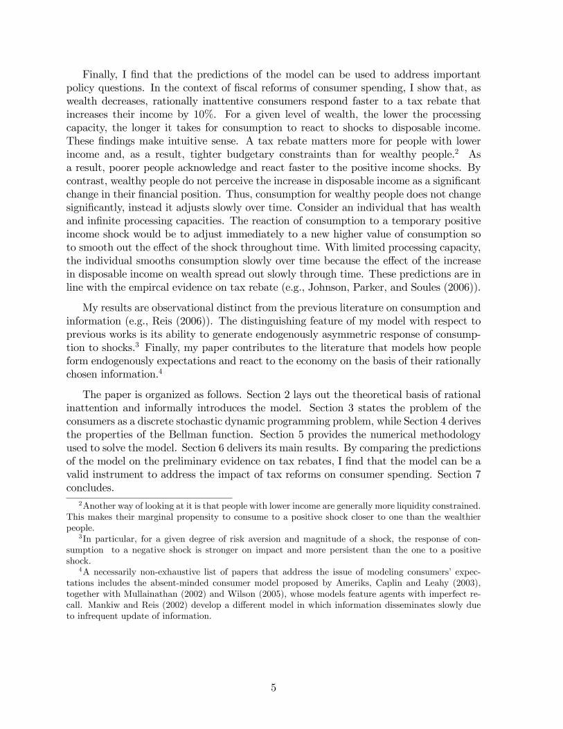
A caveat is in order. In order to explore the interaction between information �ow andcoe¢ cient of risk aversion, I solve the model in (8)-(12) information �ow by �xing theshadow cost of processing information, �, attached to (9) and let � vary endogenouslyevery period. In this section, I follow a di¤erent route. In order to clarify the mechanismsbehind Shannon capacity as a constraint for information transmission, I �x the numberof bits, �, across utilities and adjust the shadow cost � to map di¤erent coe¢ cients ofrisk aversion to the same information �ow.8 First consider u (c) = log (c). In the fullinformation case,9 the distribution g (w) is degenerate, the choice of p (ct; wt) reduces tothat of c (wt) in (8).10 The resulting optimal policy is given by

c�t (wt) = (1� �)wt + ��y: (13)

8To be more speci�c, I solve the model with CRRA consumer assuming the same parameters asthe baseline model (�;R; �y)�(0:9881; 1:012; 1; 1), the same simplex point (prior) g ( ~w) and adjusting theshadow cost of processing capacity, �, to get roughly the same information capacity (�log = 2:08 and�crra = 2:13). The latter implies that the di¤erence in allocation of probabilities within the grid areattributable solely on the coe¢ cient of risk aversion . As I will explain in more details in the solutionmethodologies, the same shadow cost (�) does deliver di¤erent information �ow (�) according to thedegree of risk aversion of the agents with more risk averse agents having higher � for a given � than lessrisk averse ones. To get �log t �crra , I set �log = 0:02 in Figure 3 while �crra = 0:08 in Figure 4.

9Or, in the wording of my model, when information �ows at in�nite rate, �!1 in (9).10More formally, for I (p (�w; �c)) ! 1, the probabilities g (w) and p (�w; �c) are degenerate. Using

10

For comparison with the case with �nite �, I plot the policy function for the (discretized)full information case as the joint distribution p (c; w) �c�(w) (c; w) with �c�(w) as the Diracmeasure. Figure 1 plots such a distribution for a 20x20 grid where the equi-spaced vectorc ranges from 0:8 to 3 and w is also equi-spaced with support in [1; 10].

02.895

5.2637.631

10

01.263

1.8422.421

30

0.05

0.1

0.15

w

pcw,Log Utility, κ→∞

c

pcw

Figure 1: Joint pdf p (c; w), high capacity.

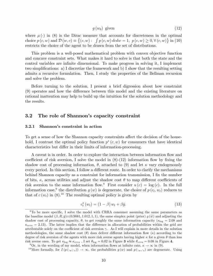
Suppose now that capacity is low. In this case, rational consumers limit their process-ing e¤ort by concentrating probability on the highest feasible value(s) of consumption.To see why, recall that consumers are risk averse (log-utility). They process the neces-sary information to learn where the boundary c � w is and avoid infeasible consumptionbundles.11 Since the Shannon capacity places high restriction on information-processing,this individual consumes roughly the same amount each period, independently of his level

Fano�s inequality (Thomas and Cover 1991),

c (I (p (�w; �c))) = c (w)

which makes the �rst order conditions for this case the full information solutions.

11The model assumes a standard No-Ponzi condition for the model (8)-(12).

11

of wealth.

01 .4 7 4

2 .4 2 13 .3 6 8

4 .3 1 65 .2 6 3

6 .2 1 07 .1 5 8

8 .1 0 59 .0 5 2

1 0

00 .9 1 6

1 .1 4 71 .3 7 9

1 .6 1 01 .8 4 2

2 .0 7 42 .3 0 5

2 .5 3 72 .7 6 8

30

0 .0 1

0 .0 2

0 .0 3

0 .0 4

0 .0 5

0 .0 6

0 .0 7

0 .0 8

w

p cw :L o g   Uti l i ty,κ= 0. 2

c

pcw

Figure 2: Joint pdf p (c; w), low capacity.

This case describes situations in which people have a vague idea of their wealth andprefer default savings/spending options (whether it is a pension plan or health insurance)rather than �guring out the exact consistency of their net worth. Figure 2 displays theresulting optimal policy. Finally, Figure 3 displays the optimal joint distribution foran intermediate case, 0 < � < 1. The �rst observation is that a person with a �niteinformation �ow tries to make p (cjw) as close to w as the information constraint allows

12

him to.

02.895

5.2637.631

10

01.263

1.8422.421

30

0.02

0.04

0.06

0.08

pcw:Log Utility, κ=2.08

Figure 3. Joint distribution p (c; w), intermediate capacity.

The second observation is that the optimal policy function for the information-constrained consumer places low weight, even no weight, on low values of consumptionfor high values of wealth. The reason why this happens depends on the utility function.A consumer with log-utility wants to maintain a consumption pro�le that is fairly smooththroughout the lifetime, as can be seen from (13). To avoid values of consumption thatare either too low or too high, he needs to be well informed about such events to re-duce the probability of their occurrence. The resulting optimal policy places a higherprobability mass on the central values of consumption and wealth.

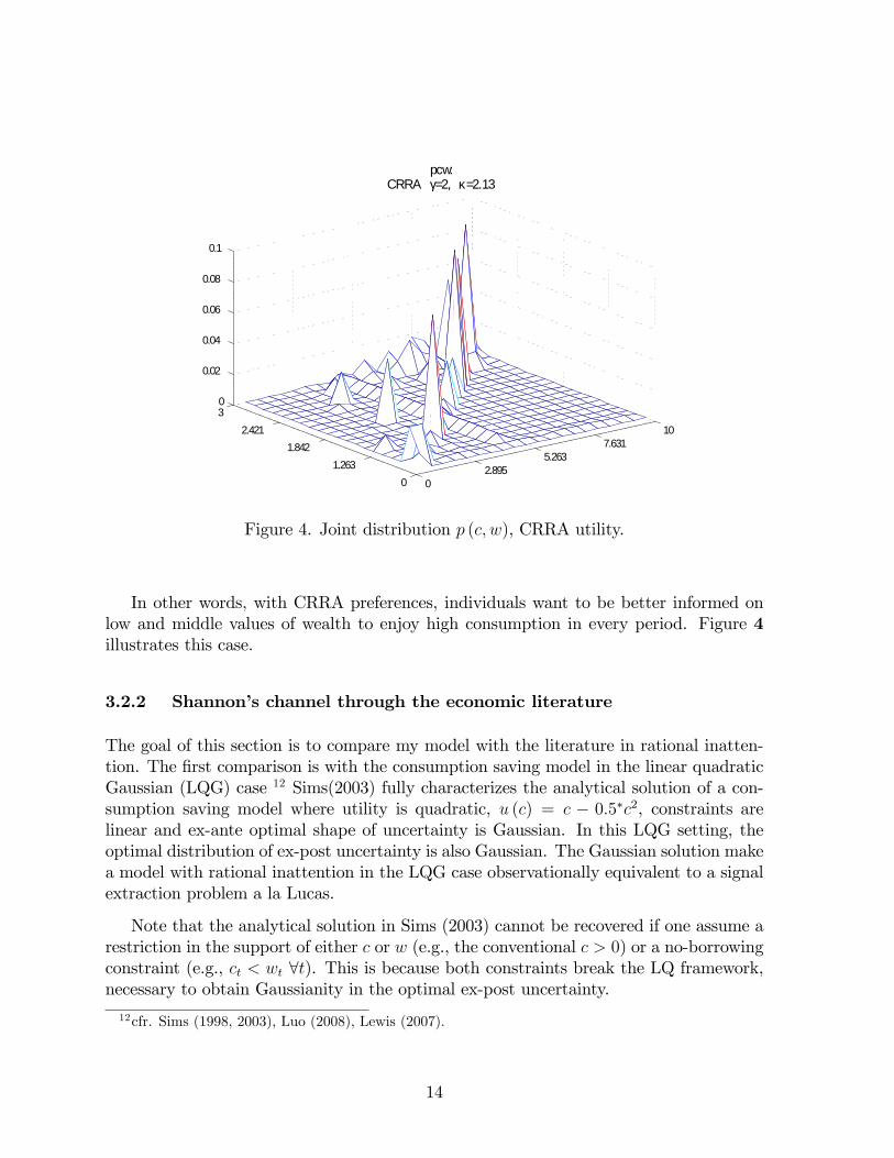
To see how the allocation of probability changes with the utility function, consider aconsumer that di¤ers from the previous only in the utility speci�cation which now assumea CRRA form, u (c) = c1� = (1� ) with = 2. As in the previous case, the optimalpolicy function still places a close-to-zero probability on low values of consumption forhigh values of wealth but now the CRRA consumer trade o¤ probabilities about modestvalues of consumption and wealth so that he can have high probability mass on highvalues of consumption when wealth is high.

13

02.895

5.2637.631

10

01.263

1.8422.421

30

0.02

0.04

0.06

0.08

0.1

pcw:CRRA γ=2, κ=2.13

Figure 4. Joint distribution p (c; w), CRRA utility.

In other words, with CRRA preferences, individuals want to be better informed onlow and middle values of wealth to enjoy high consumption in every period. Figure 4illustrates this case.

3.2.2 Shannon�s channel through the economic literature

The goal of this section is to compare my model with the literature in rational inatten-tion. The �rst comparison is with the consumption saving model in the linear quadraticGaussian (LQG) case 12 Sims(2003) fully characterizes the analytical solution of a con-sumption saving model where utility is quadratic, u (c) = c � 0:5�c2, constraints arelinear and ex-ante optimal shape of uncertainty is Gaussian. In this LQG setting, theoptimal distribution of ex-post uncertainty is also Gaussian. The Gaussian solution makea model with rational inattention in the LQG case observationally equivalent to a signalextraction problem a la Lucas.

Note that the analytical solution in Sims (2003) cannot be recovered if one assume arestriction in the support of either c or w (e.g., the conventional c > 0) or a no-borrowingconstraint (e.g., ct < wt 8t). This is because both constraints break the LQ framework,necessary to obtain Gaussianity in the optimal ex-post uncertainty.

12cfr. Sims (1998, 2003), Luo (2008), Lewis (2007).

14

The second issue with the LQG approach is that the linear quadratic approximationgives valid predictions when uncertainty is small. This is similar to the argument forlinearizing the �rst order condition of a problem and getting locally a good approximation.However, if one wants to explain an observed consumption and savings time series throughlimited processing constraints, the inertial behavior that we see in the data suggests thatuncertainty is fairly big. Thus, the tractability of the LQG framework comes at theexpense of e¤ectiveness in matching the data.

The third issue, which is the most important for the purpose of this paper, is thatrational inattention LQG models do not allow to explain di¤erent speed and amounts ofreactions of people to di¤erent news about their wealth. For instance, consumption dropsfaster following a sudden layo¤than in the event of a tax break. Moreover, the magnitudeof the change in consumption depends on people�s attitude towards risk13 and theirincome level14. The certainty equivalence framework that arises with Gaussian ex anteuncertainty and quadratic utility does not allow for endogenous di¤erentiation amongstthese events. In such a setting, the speed and amount of households�reactions to di¤erentnews are created by sources of inertia exogenous to the model. This has been one of thecriticisms to signal extraction models a la Lucas and applies also to rational inattentionLQG.15 For instance, di¤erent reactions are generated by assuming that people haveimmediate access to some signals and not others, as in Lucas (1973) or they receiveindependent information about di¤erent news, as in Mackowiak and Wiederholt (2008).In this paper, I choose another approach. I assume that information is freely availableand I do not constrain ex-ante uncertainty to be Gaussian. Moreover, I explore the linkbetween risk aversion and information-processing limits by allowing utility speci�cationsof the CRRA family.

Before this paper, Sims (2006) solves a two period model with non-Gaussian ex-anteuncertainty and CRRA preferences. Sims (2006) assumes that agents live two periods, the�rst of which they are inattentive while the second period their uncertainty is resolved.This paper focuses on a fully dynamic rational inattention model. I depart from thework of Sims (2006) in two main dimensions. The �rst is conceptual. A fully dynamicmodel with rational inattention allows the researcher to investigate time series propertiesof consumption and savings. The resulting behavior reveals endogenous noise and delaysof consumption in response to shock to income, with negative income shocks producingfaster reactions e¤ects as the risk aversion increases. The intuition for this result isthe reaction of risk adverse individuals to signals that indicate a reduction in wealthis to immediately decrease their consumption for precautionary motives while collectinginformation over time about the consistency of their net worth. Complementary to these�ndings, richer dynamic makes the model suitable to address policy questions such asreaction to �scal policy stimulus as I will show in the last section. This paper is alsodistinct from the one of Lewis (2008) . The most prominent di¤erences are that, in Lewis(2008), households do not see consumption over time and they optimize over a �nite

13cfr., e.g. Gourinchas and Parker, 2001.14cfr., e.g., Johnson, Souleles and Parker (2006).15For a discussion on the Gaussian assumption in rational inattention models see Lewis (2007).

15

horizon. Not observing consumption in turn implies that once the stream of probabilitiesis chosen at the beginning of period, the update of the beliefs is deterministic in the choiceof the signal. While Lewis (2008)�s framework does deliver upward-sloping age pro�les asaverage consumption over a �xed time length, it does not allow to study unconditionalmoments of consumption nor conditional response of consumption to shocks as in myframework.

The second contribution is methodological. A fully dynamic rational inattentionmodel involves facing an in�nite dimensional problem as displayed in (8)-(12). To workwith this framework, I developed analytical and computation tools that are suitable toaddress the dynamics of a non-LQG model.

Moreover, my results are observational distinct from the previous literature on stickyinformation (Mankiw and Reis (2002)) and consumption and information (Reis (2006)).Mankiw and Reis (2002) assume that every period an exogenous fraction of agents (�rms)obtain perfect information concerning all current and past disturbances, while all other�rms set prices based on old information. Reis (2006) shows that a model with a �xedcost of obtaining perfect information can provide a microfoundation for this kind of slowdi¤usion of information. My model di¤ers from the literature on inattentiveness in that Iassume that information is freely available in each period but the bounds on informationprocessing given by the Shannon channel force consumers to choose the scope of theirinformation within the limit of their capacity. The interaction of information �ow andrisk aversion in my model delivers endogenous asymmetry in the response of consumptionto shocks both in terms of speed and amount. This prediction constitutes a distinguishingfeature of my model with respect to the literature of inattentiveness and, more generally,to the consumption-saving literature.

4 Solution Methodology

4.1 Discretizing the Framework

I consider wealth and consumption as de�ned on compact sets. In particular, admissibleconsumption pro�les belong to c � fcmin; :::; cmaxg : Likewise, wealth has support w �fwmin; :::; wmaxg. I identify by j the elements of set c and by i the elements in w: Iapproximate the state of the problem, i.e., the distribution of wealth by using the simplex:

De�nition The set � of all mappings g : w ! R ful�lling g (w) � 0 for all w 2 wand

Pw2w

g (w) = 1 is called a simplex. Elements w of w are called vertices of

the simplex �, functions g are called points of �.

Let jSj be the dimension of the belief simplex which approximates the distribution

g (w) and let � �(g 2 RjSj : g (i) � 0 for all i

jSjPi=1

g (i) = 1

)denote the set of all prob-

16

ability distribution on �. The initial condition for the problem is g (w0) :

The consumer enters each period choosing the joint distribution of consumption and�nancial possibilities. From the previous section, the control variable for the discretizedset up as the probability mass function Pr (w; c) where c 2 c and w 2 w, constrainedto belong to the set of distributions. Given g (w0) and Pr (ct; wt) and the observation ofct consumed in period t; the belief state is updated using Bayesian conditioning:

g0�wt+1jct

�=Xwt2w

T (wt+1;wt; ct) Pr (wtjct) (14)

where T (:) is a discrete counterpart of the transition function ~T (:). Note that ~T (:) is adensity function on the real line while T (:) is a density function on a discrete set withcounting measure. The processing constraint, in terms of the discrete mutual informationbetween state and actions, is:

It (p (�ct ; �wt)) =Xwt2w

Xct2c

Pr (ct; wt)

�log

Pr (ct; wt)

p (ct) g (wt)

�(15)

The interpretation of (15) is akin to its continuous counterpart. The capacity of theagents to process information is constrained by a number, ��, which denotes the upperbound on the rate of information �ow between the random variables C and W 16 in timet. Finally, the objective function (8) in the discrete world amounts to

maxfp(wt;ct)g1t=0

E0

( 1Xt=0

�t

" Xwt2w

Xct2w

�c1� t

1�

�Pr (ct; wt)

#����� I0): (16)

4.2 Recursive Formulation

The purpose of this section is to show that the discrete dynamic programming problemhas a solution and to recast it into a Bellman recursion. To show that a solution ex-ists, �rst note that the set of constraints for the problem is a compact-valued concavecorrespondence. Second, I need to show that the state space is compact. Compactnesscomes from the curvature of the utility function and the fact that the belief space has abounded support in [0; 1]. The compact domain of the state and the fact that Bayesianconditioning for the update preserves the Markovianity of the belief state ensures thatthe transition Q : (w � Y � B ! [0; 1]) and (14) has the Feller property. Then, theconditions for applying the Theorem of the Maximum are ful�lled which guarantees theexistence of a solution. In the next section, I provide su¢ cient conditions to guaranteeuniqueness.

Casting the problem of the consumer in a recursive Bellman equation formulation,

16Recall from the argument in Section 2.1 that both W and C are random variables before thehousehold has acquired and processed any information.

17

the full discrete-time Markov program amounts to:

V (g (wt)) = maxPr(ct;wt)

26664Xwt2w

Xct2c

u (ct) Pr (ct; wt)

!+

+�P

wt2w

Xct2c

V�g0cjt(wt+1)

�Pr (ct; wt)

37775 (17)

subject to:

(� :)

�t = It (p (�ct ; �wt)) =Xwt2w

Xct2c

Pr (ct; wt)

�log

Pr (ct; wt)

p (ct) g (wt)

�(18)

g0�wt+1jct

�=Xwt2w

T (wt+1;wt; ct) Pr (wtjct) (19)

Xct2c

Pr (ct; wt) = g (wt) (20)

1 � Pr (ct; wt) � 0 8 (ct; wt) 2 B; 8t (21)

where B � f(ct; wt) : wt � ct; 8ct 2 c;8wt 2 w, 8tg and � is the Lagrange multiplier(shadow cost) associated to (18).

The Bellman equation in (17) takes up as its argument the marginal distributionof wealth g (wt) and uses as the control variable the joint distribution of wealth andconsumption, Pr (ct; wt). The latter links the behavior of the agent with respect toconsumption (c), on one hand, and income (w) on the other, hence specifying the actionsover time. The �rst term on the right hand side of (17) is the utility function u (:). The

second term,P

wt2w

Xct2c

V�g0cjt(wt+1)

�Pr (ct; wt), represents the expected continuation

value of being in state g (:) discounted by the factor � = 1=R = 0:9881. This correspondsto interest rate R = 1:012 which gives an annualized gross real rate of investment R^4 =1:0489, with a quarterly frequency of the data. The expectation is taken with respect tothe endogenously chosen distribution Pr (ct; wt). I have discussed the relations in (18)-(21) earlier. Moreover, I appended the equation in (20) which constrains the choice ofthe distribution to be consistent with the initial prior g (wt) :

Next, I analyze the main properties of the Bellman recursion (17) and derive condi-tions under which it is a contraction mapping and show that the mapping is isotone.

4.3 Properties of the Bellman Recursion

To prove that the value function is a contraction and an isotonic mapping, I shall in-troduce the relevant de�nitions. Let me restrict attention to choices of probability dis-tributions that satisfy the constraints (18)-(21). To make the notation more compact,let p � Pr (cjjwi), 8cj 2 c, 8wi 2 w and let � be the set that contains (18)-(21). Iintroduce the following de�nitions:

18

D1. A control probability distribution p � Pr (ci; wj) is feasible for the problem (17)-(21) if p 2 �: Let jW j be the cardinality of w and let

G �

8<:g 2 RjW j : g (wi) � 0; 8i;jW jXi=1

g (wi) = 1

9=;denote the set of all probability distributions on w. An optimal policy has a valuefunction that satis�es the Bellman optimality equation in (17):

V � (g) = maxp2�

"Xw2w

Xc2c

u (c) p (cjw)!g (w) + �

Xw2w

Xc2c

(V � (g0c (�))) p (cjw) g (w)#

(22)The Bellman optimality equation can be expressed in value function mapping form.Let V be the set of all bounded real-valued functions V on G and let h : G �w �(w � c)� V ! R be de�ned as follows:

h (g; p; V ) =Xw2w

Xc2c

u (c) p (cjw)!g (w) + �

Xw2w

Xc2c

(V (g0c (�))) p (cjw) g (w) :

De�ne the value function mapping H : V ! V as (HV ) (g) = maxp2� h (g; p; V ).

D2. A value function V dominates another value function U if V (g) � U (g) for allg 2 G:

D3. A mapping H is isotone if V , U 2 V and V � U imply HV � HU:

D4. A supremum norm of two value functions V , U 2 V over G is de�ned as

jjV � U jj = maxg2G

jV (g)� U (g)j

D5. A mapping H is a contraction under the supremum norm if for all V , U 2 V,

jjHV �HU jj � � jjV � U jj

holds for some 0 � � < 1:

Endowed with these notion, it is possible to derive some properties of the solution tothe Bellman equation.

First, note that the uniqueness of the solution to which the value function convergesto requires concavity of the constraints and convexity of the objective function. It isimmediate to see that all the constraints but (18) are actually linear in p (c; w) andg (w). For (18), the concavity of p (c; w) is guaranteed by Theorem (16.1.6) of Thomasand Cover (1991). The concavity of g (w) is the result of the following:

Lemma 1. For a given p (cjw) ; the expression (18) is concave in g (w).

19

Proof. See Appendix B.

Next, I need to prove the convexity of the value function and the fact that the valueiteration is a contraction mapping. All the proofs are in Appendix A.

Proposition 1. For the discrete Rational Inattention Consumption Saving value recur-sion H and two given functions V and U , it holds that

jjHV �HU jj � � jjV � U jj ;with 0 � � < 1 and jj:jj the supreme norm. That is, the value recursion H is acontraction mapping.

Proposition 1 can be explained as follows. The space of value functions de�nes avector space and the contraction property ensures that the space is complete. Therefore,the space of the value functions together with the supreme norm form a Banach space;the Banach �xed-point theorem ensures (a) the existence of a single �xed point and (b)that the value recursion always converges to this �xed point (see Theorem 6 of Alvarezand Stockey, 1998 and Theorem 6.2.3 of Puterman, 1994).

Corollary For the discrete Rational Inattention Consumption Saving value recursion Hand two given functions V and U , it holds that

V � U =) HV � HU

that is the value recursion H is an isotonic mapping.

The isotonic property of the value recursion ensures that the value iteration convergesmonotonically.

These theoretical results establish that in principle there is no barrier in de�ningvalue iteration algorithms for the Bellman recursion for the discrete rational inattentionconsumption-savings model.

5 Numerical Technique and its Predictions

I solve the model by transforming the underlying partially observable Markov decisionprocess into an equivalent, fully observable Markov decision process with a state spacethat consists of all probability distributions over the core 17 state of the model (wealth).

For a model with n core states, w1; ::; wn, the transformed state space is the (n� 1)-dimensional simplex, or belief simplex. Expressed in plain terms, a belief simplex is apoint, a line segment, a triangle or a tethraedon in a single, two, three or four-dimensionalspace, respectively. Formally, a belief simplex is de�ned as the convex hull18 of belief17The state of the model is a probability distribution of wealth, i.e., g (w). For lack of a better

alternative, I call core state the random variable w whose distribution is the state of the model. Thisnomenclature is borrowed from information theory and AI literature. cfr. Puterman (1994) .18A convex hull of a set of points is de�ned as the closure of the set under convex combination.

20

states from an a¢ nely independent19 set B. The points of B are the vertices of the beliefsimplex. The convex hull formed by any subset of B is a face of the belief simplex. Toaddress the issue of dimensionality in the state space of my model, I use a grid-basedapproximation approach. The idea of a grid based approach is to use a �nite grid todiscretize the uncountably in�nite continuous state space. The implementation has thefollowing steps: I place a �nite grid over the simplex point, I compute the values forpoints in the grid, and I use a kernel regression to interpolate solution points that falloutside the grid.

5.1 Belief Simplex and Dynamic Programming

If full information were available, previous history of the process would be irrelevant tothe problem. However, because the consumer cannot completely observe wealth, he mayrequire all the past information about the system to behave optimally. The most generalapproach is to keep track of the entire history of his previous consumption purchases upto time t, denoted Ht = fg0; c1; ::; ct�1g. For any given initial state probability distribu-tion g0, the number of possible histories is (jCj)t with C denoting the set of consumptionbehavior up to time t. This number goes to in�nity as the decision horizon approachesin�nity, which makes this method of representing history useless for in�nite-horizon prob-lems.

To overcome this issue, Astrom (1965) proposed an information state approach. It isbased upon the idea that all the information needed to act optimally can be summarizedby a vector of probabilities over the system, the belief state. Let g (w) denote theprobability that the wealth is in state w 2 w where w is assumed to be a �nite set.Probability distributions such as g (w) that are de�ned on �nite sets are in fact simplices.Let n be the possible values that w can assume. The discretization of the core state is anequi-spaced grid with n = 20 values of w ranging from 1 to 10. The points in the simplex� are n distinct values for the marginal pdf g (w) in the interval I � [0; 1]. The simplexis constructed using uniform random samples from the unit simplex. The reason why Iuse this methodology is that it is computationally faster than non-uniform grid and it isable to handle higher dimensional space.20 In my model, each point in the simplex is ann-array whose column contains m random values in the [0; 1] range and whose sum perrow is 1. To span the simplex I use m = (n� 1)!.21 The distribution of values withinthe simplex is uniform in the sense that it has the conditional probability of a uniformdistribution over the whole m-cube, given that the sum per row is 1. The algorithmcalls three types of random processes that determine the placement of random points

19A set of belief states fgig, 1 � i � z is called a¢ nely independent when the vectors fgi � gzg arelinearly independent for 1 � i � z.20At least compared to the ndgrid library functions in Matlab. This is because the algorithm creates

the simplex directly while when using ndgrid it is necessary to de�ne a uniform grid over the whole n�1space and then sectioning the resulting grid so that each simplex point sum to one.21With n = 20, the proposed sampling produces the same results for sample size of m = (n� k)!, for

k = 1; ::; 5. I have not tried cases with k < 5: When k > 1, even if the algorithm produces the sameresults it takes longer to converge (about 3 minutes more per iteration).

21

in the n � 1�dimensional simplex. The �rst process considers values uniformly withineach simplex. The second random process selects samples of di¤erent types of simplex inproportion to their volume. Finally, the third process implements a random permutationin order to have an even distribution of simplex choices among types.

For each simplex point, I initialize the corresponding joint distribution of consumptionc and wealth w. I assume n = 20 equi-spaced values for c ranging in c � [0:8; 3]. Thevalues in c are chosen so that w is about 3 times c, roughly consistent with individualdata on consumption and wealth.

Let core states and behavior states be sorted in descending order. I impose the con-straint c < w,22. Then, given the symmetry in the dimensionality of c and w, the jointdistribution of consumption and wealth for a given multidimensional grid point is squarematrix with rows corresponding to levels of consumption. Summing the matrix per rowresults in the marginal distribution of consumption, p (c). Likewise, the columns of thematrix correspond to levels of wealth. Evaluating the sum per columns of the matrixamounts to the marginal pdf of wealth, g (w). Given the initial belief simplex, its succes-sor belief states can be determined by Bayesian conditioning at each multidimensionalpoint of the simplex and gives the expression:

g (w0jc) =Xi

T (w0;wi; c) Pr (wijc) = Pr (w0jc) : (23)

Let V be the set of all bounded real-valued function V on G. Then, the Bellmanoptimality equation of the household is described by (17)-(21).

Without loss of generality, I restrict the columns of the matrix Pr (c; w) to sum to themarginal pdf of wealth in the main diagonal. Moreover, because some of the values of themarginal g (w) per simplex-point are exactly zero given the de�nition of the envelope forthe simplex, I constrain the choices of the joint distributions corresponding to those valuesto be zero. This handling of the zeroes makes the parameter vector being optimized overhave di¤erent lengths for di¤erent rows of the simplex. Hence the degrees of freedomin the choice of the control variables for simplex points vary from a minimum of 0 to amaximum of n�(n�1)

2.23 Once the belief simplex is set up, I initialize the joint probability

distribution of consumption and wealth per belief point and solve the program of thehousehold by backward induction iterating on the value function V (g (w)). To map the

22The constraint c < w makes economic sense since there is no borriwng in this economy. To encodethis constraint without complicating the model, one may assume that �t in (18) is the capacity left afterth consumer has processed his spending limits.Note also that this constraint is computationally convenient reducing the number of choice variables

from n2 = 400 to n(n+1)2 = 210 per iteration.

23To illustrate this point, two example in which the 0-degree of freedom and the n�(n�1)2 -degree of

freedom occur are as follows. Suppose for simplicity that n = 3: Then, if a simplex point has realization

g � f1; 0; 0g the joint pdf of consumption and wealth turns out to be p (c; w) =

24 1 0 00 00

35 leavingzero degrees of freedom. If, instead, e.g., g �

�13 ;

13 ;

13

, the consumers has to choose 3�(2)

2 = 3 points onthe joint distribution, fp1; p2; p3g placed as:

22

�ner state space into Matlab possibilities, I interpolate the value function with the newvalues of (23) using a kernel regression of V (�) into g0 (w0ja) : I use an Epanechnikovkernel with smoothing parameter h = 2:7. 24 A kernel regression approximates theexact non linear value function in (17) with a piece-wise linear function. The followingpropositions illustrate this point.

Proposition 2. If the utility is CRRA with a parameter of risk aversion 2 (0;+1)and if Pr (cj; wi) satis�es (18)-(21), then the optimal n�step value function Vn (g)de�ned over G can be expressed as:

Vn (g) = maxf�ingi

Xi

�n (wi) g (wi)

where the �� vectors, � : w ! R, are jW j �dimensional hyperplanes.

Intuitively, each �n�vector corresponds to a plan and the action associated with agiven �n�vector is the optimal action for planning horizon n for all priors that have sucha function as the maximizing one. With the above de�nition, the value function amountsto:

Vn (g) = maxf�ingi

�in; g

�;

and thus the proposition holds.

Using the above proposition and the fact that the set of all consumption pro�lesP � fc < w : p (c) > 0g is discrete, it is possible to show directly the convex propertiesfor the value function. For �xed �in�vectors, the h�in; gi operator is linear in the beliefspace. Therefore, the convex property is given by the fact that Vn is de�ned as themaximum of a set of convex (linear) functions and, thus, obtains a convex function as aresult. The optimal value function V � is the limit for n!1 and, becuase all the Vn areconvex function, so is V �.

Proposition 3. Assuming the CRRA utility function and the conditions of Proposition1, let V0 be an initial value function that is piecewise linear and convex. Thenthe ith value function obtained after a �nite number of update steps for a rationalinattention consumption-saving problem is also �nite, piecewise linear and convex(PCWL).

p (c; w) =

24 13 p1 p2

13 p3

13

35 :24Epanechnikov kernel is an optimum choice for smoothing because it minimizes asymptotic mean

integrated squared error (cfr. Marron, J. S. and Nolan, D. (1988)). I use the algorithm proposed inBeresteanu, A. and C. F. Manski (2000) and experiement with smoothing paramter h 2 [0:3 : 0:3 : 4:2].For the characteristics of the problem, and the optimization routine used (csminwel), for di¤erent spec-i�cation of utility functions and Lagrange multiplier �, the parameter h = 2:7 performs best in terms ofcomputational time and convergence of the value function.

23

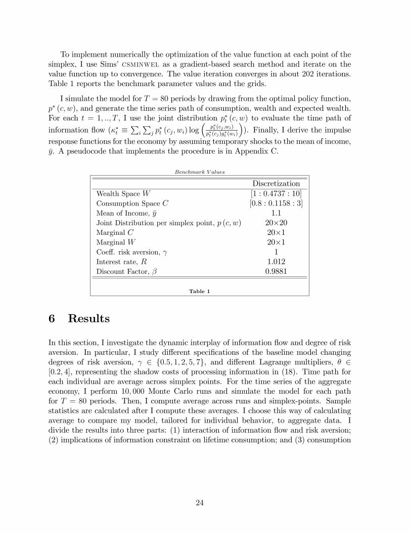
To implement numerically the optimization of the value function at each point of thesimplex, I use Sims�csminwel as a gradient-based search method and iterate on thevalue function up to convergence. The value iteration converges in about 202 iterations.Table 1 reports the benchmark parameter values and the grids.

I simulate the model for T = 80 periods by drawing from the optimal policy function,p� (c; w), and generate the time series path of consumption, wealth and expected wealth.For each t = 1; ::; T , I use the joint distribution p�t (c; w) to evaluate the time path of

information �ow (��t �P

i

Pj p

�t (cj; wi) log

�p�t (cj ;wi)

p�t (cj)g�t (wi)

�). Finally, I derive the impulse

response functions for the economy by assuming temporary shocks to the mean of income,�y. A pseudocode that implements the procedure is in Appendix C.

Benchmark V alues

DiscretizationWealth Space W [1 : 0:4737 : 10]Consumption Space C [0:8 : 0:1158 : 3]Mean of Income, �y 1.1Joint Distribution per simplex point, p (c; w) 20�20Marginal C 20�1Marginal W 20�1Coe¤. risk aversion, 1Interest rate, R 1.012Discount Factor, � 0.9881

Table 1

6 Results

In this section, I investigate the dynamic interplay of information �ow and degree of riskaversion. In particular, I study di¤erent speci�cations of the baseline model changingdegrees of risk aversion, 2 f0:5; 1; 2; 5; 7g, and di¤erent Lagrange multipliers, � 2[0:2; 4], representing the shadow costs of processing information in (18). Time path foreach individual are average across simplex points. For the time series of the aggregateeconomy, I perform 10; 000 Monte Carlo runs and simulate the model for each pathfor T = 80 periods. Then, I compute average across runs and simplex-points. Samplestatistics are calculated after I compute these averages. I choose this way of calculatingaverage to compare my model, tailored for individual behavior, to aggregate data. Idivide the results into three parts: (1) interaction of information �ow and risk aversion;(2) implications of information constraint on lifetime consumption; and (3) consumption

24

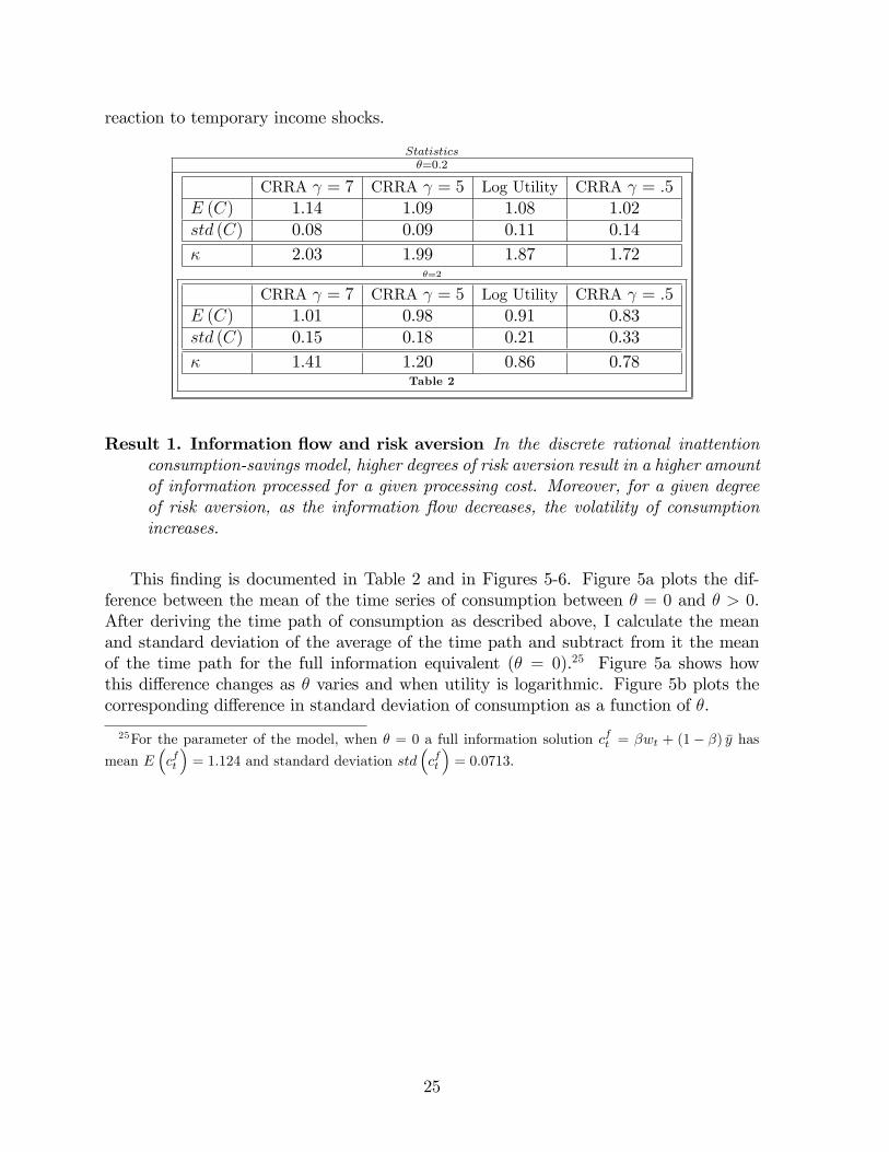
reaction to temporary income shocks.

Statistics�=0:2

CRRA = 7 CRRA = 5 Log Utility CRRA = :5E (C) 1.14 1.09 1.08 1.02std (C) 0.08 0.09 0.11 0.14� 2.03 1.99 1.87 1.72

�=2

CRRA = 7 CRRA = 5 Log Utility CRRA = :5E (C) 1.01 0.98 0.91 0.83std (C) 0.15 0.18 0.21 0.33� 1.41 1.20 0.86 0.78

Table 2

Result 1. Information �ow and risk aversion In the discrete rational inattentionconsumption-savings model, higher degrees of risk aversion result in a higher amountof information processed for a given processing cost. Moreover, for a given degreeof risk aversion, as the information �ow decreases, the volatility of consumptionincreases.

This �nding is documented in Table 2 and in Figures 5-6. Figure 5a plots the dif-ference between the mean of the time series of consumption between � = 0 and � > 0.After deriving the time path of consumption as described above, I calculate the meanand standard deviation of the average of the time path and subtract from it the meanof the time path for the full information equivalent (� = 0).25 Figure 5a shows howthis di¤erence changes as � varies and when utility is logarithmic. Figure 5b plots thecorresponding di¤erence in standard deviation of consumption as a function of �.

25For the parameter of the model, when � = 0 a full information solution cft = �wt + (1� �) �y hasmean E

�cft

�= 1:124 and standard deviation std

�cft

�= 0:0713:

25

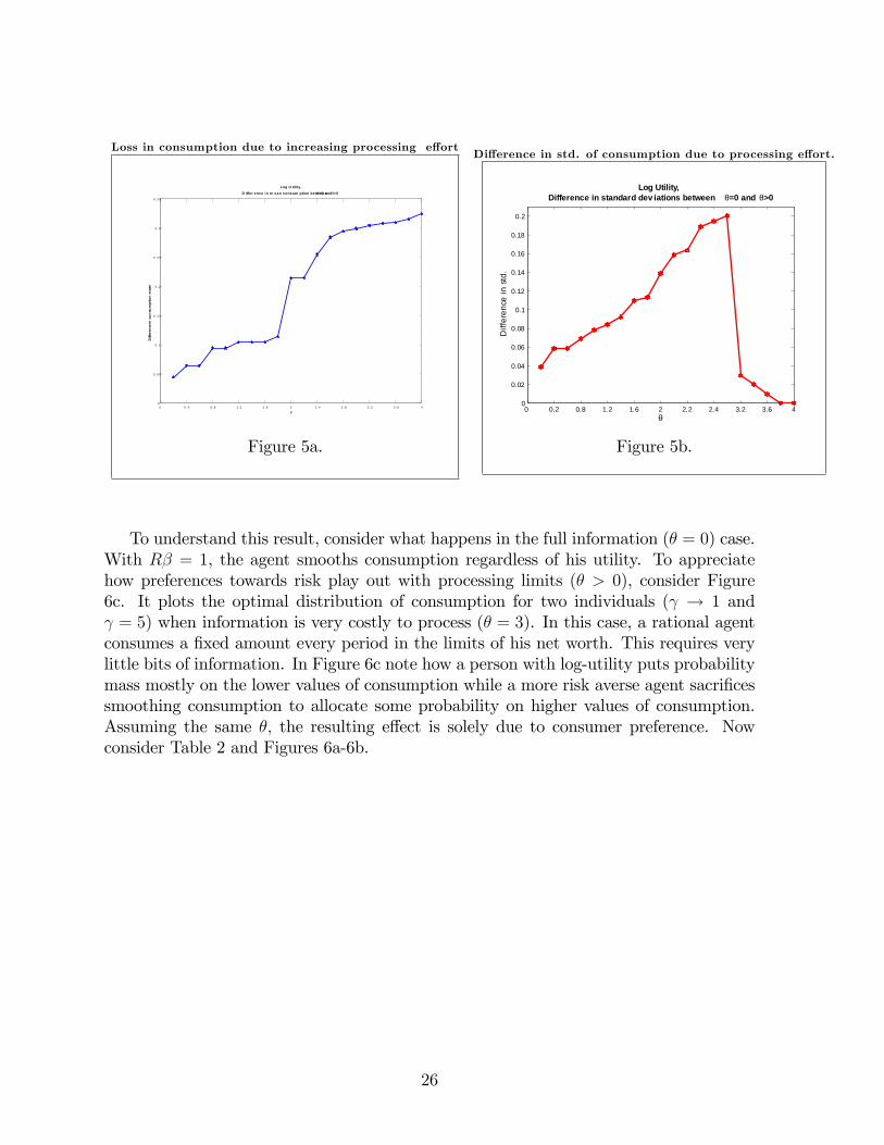
Loss in consumption due to increasing processing e¤ort

0 0 .4 0 .8 1 .2 1 .6 2 2 .4 2 .8 3 .2 3 .6 40

0 .0 5

0 .1

0 .1 5

0 .2

0 .2 5

0 .3

0 .3 5

θ

Diff

eren

ce in

 co

nsu

mp

tion

 mea

n

Log U tility,

D iffer ence in m ean consum ption betw eenθ=0 andθ>0

Figure 5a.

Di¤erence in std. of consumption due to processing e¤ort.

0 0.2 0.8 1.2 1.6 2 2.2 2.4 3.2 3.6 40

0.02

0.04

0.06

0.08

0.1

0.12

0.14

0.16

0.18

0.2

Log Utility,Difference in standard dev iations between θ=0 and θ>0

θ

Diff

eren

ce in

 std

.

Figure 5b.

To understand this result, consider what happens in the full information (� = 0) case.With R� = 1, the agent smooths consumption regardless of his utility. To appreciatehow preferences towards risk play out with processing limits (� > 0), consider Figure6c. It plots the optimal distribution of consumption for two individuals ( ! 1 and = 5) when information is very costly to process (� = 3). In this case, a rational agentconsumes a �xed amount every period in the limits of his net worth. This requires verylittle bits of information. In Figure 6c note how a person with log-utility puts probabilitymass mostly on the lower values of consumption while a more risk averse agent sacri�cessmoothing consumption to allocate some probability on higher values of consumption.Assuming the same �; the resulting e¤ect is solely due to consumer preference. Nowconsider Table 2 and Figures 6a-6b.

26

Marginal Distribution of Consumption, Log Utility

0 0.91 1.15 1.38 1.61 1.84 2.07 2.30 2.53 2.760

0.05

0.1

0.15

0.2

0.25

θ=2

θ=0.2

Figure 6a.

Marginal Distribution of Consumption, CRRA =5

0.91 1.14 1.37 1.61 1.84 2.07 2.42 2.65 2.76 30

0.05

0.1

0.15

0.2

0.25

Consumption

Pro

babi

lity

θ=0.2

θ=2

Figure 6b.

Marginal Distribution of Consumption, �=3

0.91 1.15 1.37 1.61 1.84 2.07 2.30 2.53 2.76 30

0.05

0.1

0.15

0.2

0.25

0.3

0.35

0.4

0.45

0.5

Consumption

Pro

babi

lity

γ=5

Log Utility

Figure 6c.

When � = 2, people select how much information they want to process and whichvalues of wealth to be better informed about according to their utility. Also in this case,the higher the degree of risk aversion, the higher the quest for information (�). Thisis exactly what Table 2 shows. In the table, the higher the coe¢ cient of risk aversion, , the higher the information collected by the agent, �, and the higher the mean ofconsumption. The same story can be told in terms of probability distribution as in 6a-6c. For a given level of �, a person with log utility would be better informed on extremevalues of wealth to avoid such values. This knowledge makes it possible to assign high

27

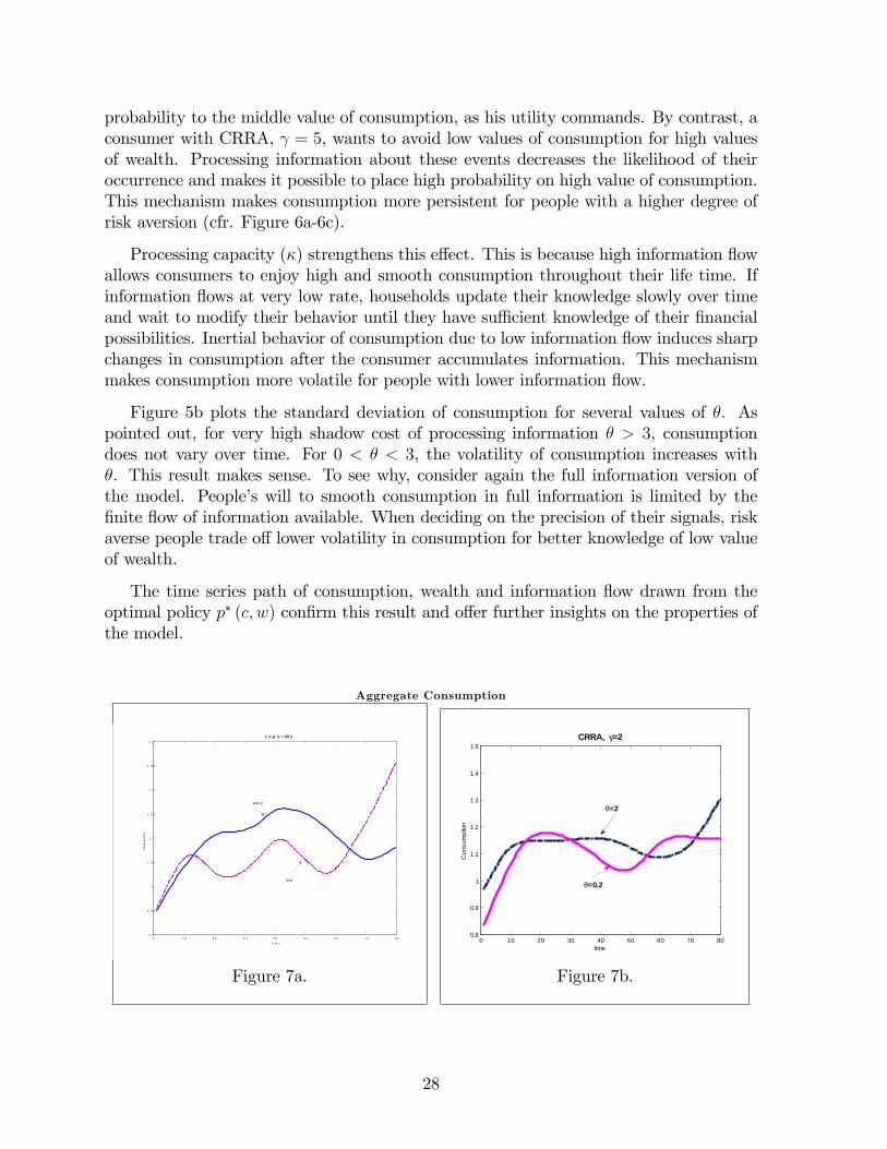
probability to the middle value of consumption, as his utility commands. By contrast, aconsumer with CRRA, = 5, wants to avoid low values of consumption for high valuesof wealth. Processing information about these events decreases the likelihood of theiroccurrence and makes it possible to place high probability on high value of consumption.This mechanism makes consumption more persistent for people with a higher degree ofrisk aversion (cfr. Figure 6a-6c).

Processing capacity (�) strengthens this e¤ect. This is because high information �owallows consumers to enjoy high and smooth consumption throughout their life time. Ifinformation �ows at very low rate, households update their knowledge slowly over timeand wait to modify their behavior until they have su¢ cient knowledge of their �nancialpossibilities. Inertial behavior of consumption due to low information �ow induces sharpchanges in consumption after the consumer accumulates information. This mechanismmakes consumption more volatile for people with lower information �ow.

Figure 5b plots the standard deviation of consumption for several values of �. Aspointed out, for very high shadow cost of processing information � > 3, consumptiondoes not vary over time. For 0 < � < 3, the volatility of consumption increases with�. This result makes sense. To see why, consider again the full information version ofthe model. People�s will to smooth consumption in full information is limited by the�nite �ow of information available. When deciding on the precision of their signals, riskaverse people trade o¤ lower volatility in consumption for better knowledge of low valueof wealth.

The time series path of consumption, wealth and information �ow drawn from theoptimal policy p� (c; w) con�rm this result and o¤er further insights on the properties ofthe model.

Aggregate Consumption

0 1 0 2 0 3 0 4 0 5 0 6 0 7 0 8 00 . 9

0 . 9 5

1

1 . 0 5

1 . 1

1 . 1 5

1 . 2

1 . 2 5

1 . 3

t i m e

Cons

umpt

ion

L o g  U t ilit y

θ= 0 .2

θ= 2

Figure 7a.

0 10 20 30 40 50 60 70 800.8

0.9

1

1.1

1.2

1.3

1.4

1.5

time

Con

sum

ptio

n

CRRA, γ=2

θ=2

θ=0.2

Figure 7b.

28

Aggregate Consumption and Information Flow

0 20 40 60 800.8

1

1.2

1.4

 Con

sum

ptio

n

time

θ=0.2, Log Utility

0 20 40 60 800.2

0.4

0.6

0.8

κ

0 20 40 60 800.8

1

1.2

1.4

 Con

sum

ptio

n

time

θ=2, Log Utility

0 20 40 60 800.55

0.6

0.65

0.7

κ

0 20 40 60 800.5

1

1.5

 Con

sum

ptio

n

time

θ=0.2, CRRA γ=2

0 20 40 60 800.55

0.6

0.65

κ0 20 40 60 80

0.9

1

1.1

1.2

1.3

1.4

 Con

sum

ptio

ntime

θ=2, CRRA γ=2

0 20 40 60 800.5

0.55

0.6

0.65

0.7

0.75

κ

Figure 7c.

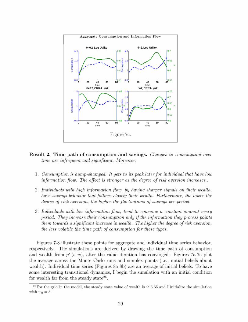
Result 2. Time path of consumption and savings. Changes in consumption overtime are infrequent and signi�cant. Moreover:

1. Consumption is hump-shamped. It gets to its peak later for individual that have lowinformation �ow. The e¤ect is stronger as the degree of risk aversion increases..

2. Individuals with high information �ow, by having sharper signals on their wealth,have savings behavior that follows closely their wealth. Furthermore, the lower thedegree of risk aversion, the higher the �uctuations of savings per period.

3. Individuals with low information �ow, tend to consume a constant amount everyperiod. They increase their consumption only if the information they process pointsthem towards a signi�cant increase in wealth. The higher the degree of risk aversion,the less volatile the time path of consumption for these types.

Figures 7-8 illustrate these points for aggregate and individual time series behavior,respectively. The simulations are derived by drawing the time path of consumptionand wealth from p� (c; w), after the value iteration has converged. Figures 7a-7c plotthe average across the Monte Carlo runs and simplex points (i.e., initial beliefs aboutwealth). Individual time series (Figures 8a-8b) are an average of initial beliefs. To havesome interesting transitional dynamics, I begin the simulation with an initial conditionfor wealth far from the steady state26.

26For the grid in the model, the steady state value of wealth is �= 5:65 and I initialize the simulationwith w0 = 3.

29

Individual consumption

0 10 20 30 40 50 60 700.8

1

1.2

1.4

1.6

1.8

time

cons

umpt

ion

Log Utility

0 10 20 30 40 50 60 700.8

1

1.2

1.4

1.6

1.8

time

cons

umpt

ion

CRRA Utility, γ=2

θ=0.2

θ=2

Figure 8a.

Individual savings and wealth

0 20 40 60 802

3

4

5

6

7

 wea

lth

t ime

Log Utility, θ=0.2

0 20 40 60 801

2

3

4

5

6

 sav

ings

0 20 40 60 800

5

10

 wea

lth

t ime

Log Utility, θ=2

0 20 40 60 800

5

10

 sav

ings

0 20 40 60 800

2

4

6

8

 wea

lth

t ime

CRRA γ=2, θ=0.2

0 20 40 60 80­2

0

2

4

6

 sav

ings

0 20 40 60 802

4

6

8

10

 wea

lth

t ime

CRRA γ=2, θ=2

0 20 40 60 800

2

4

6

8

 sav

ings

Figure 8b.

To appreciate the results, consider what would happen with full information. In sucha case, consumption smoothing (R� = 1) implies an immediate (T = 1) adjustment ofconsumption to its long-run optimal values and no transient behavior. Thus, in that casefrom T = 2 onwards, the simulations lead to a constant time path. Now consider Figures7(a-c)-8(a,b). The hump in consumption comes from Result 1 and a simple intuition:information-constrained people are cautious (degree of risk aversion � 1), consume alittle and collect information about wealth before they change consumption. For a �xed�, the more risk averse they are (cfr. Figure 7a with log utility and Figure 7b with CRRA, = 2), the longer they wait before increasing their consumption. This inertial behaviorin consumption leads to an increase in savings and, as a result, in wealth (cfr. Figure8a-8b). Processed information keeps signaling the increase in wealth until householdsrealize that they are wealthy enough to increase their consumption. Thus, the hump inconsumption is the mirrored image of the rise (until people know they rich) and fall (oncepeople know they are rich) in wealth. Note that, depending on the history of incomeshocks, consumption can have more than one hump in its path. To see why, consider ahigh realization of income occurring after a hump in consumption. Over time, signalsabout wealth convey such information, consumers start saving and history as well ashumps repeat themselves. These e¤ects are enhanced by the shadow cost of processinginformation, �, with higher costs forcing long periods of inertia in consumption followedby sizeable changes. Note also the relationship between consumption and information�ow (Figure 7c): risk averse agents would rather push forward consumption in times inwhich they are processing information about wealth. Finally, note from 7(a-b)-8(a,b)how the peak in consumption occurs later for an individual with higher degree of riskaversion and lower information �ow. The rationale for this result is that more cautiouspeople wait to be better informed about their wealth before modifying their consumption

30

behavior. In particular, since a consumer with CRRA utility ( = 2) chooses to be betterinformed about low values of wealth than a log utility consumer (cfr. Figures 7a and7b), he processes news about high value of wealth slower than his log counterpart. Theresulting additional savings for precautionary motives are triggered by both the curvatureof the utility function and the bound on information-processing constraint.

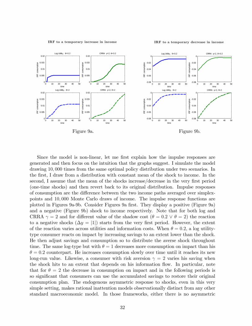
The last result comes from studying how consumers with limited processing capacityreact to temporary shocks to income (y). Before stating the result, it is worth comparingto the predictions of standard consumption-saving literature. With full information,the response of consumption to either negative and positive temporary income shocksare immediate: consumption adjust in period T = 0 to an amount exactly equal to thediscounted present value of the shock, j�yj. This is the case regardless whether the shockis adverse or favorable, so long as the absolute value of these shocks match. The sameholds true under certainty-equivalence with a linear constraints and quadratic utility(LQ) framework. With risk averse agents and information-processing limits, it happensthat:

Result 3. Persistent stickiness and asymmetric response to shocks. Consumption�sresponse to temporary �uctuations of wealth is asymmetric: Negative shocks triggera sharper reaction and higher persistence of consumption than positive ones.

The logic behind this result is easily understood by considering the interdependenceof information �ow and coe¢ cient of risk aversion. A risk averse person is more likelyto be a¤ected by negative events than positive ones. As soon as he receives signals thathis wealth is lower than what he thought, he reacts by decreasing his consumption. Thechange in behavior and its persistence are more consistent the more risk averse and unin-formed the consumer is. This occurs because consumers wait to gather more informationbefore changing their behavior and, in the meanwhile, build up a savings bu¤er. Thus,the temporary change in income propagates slowly over time. A positive temporaryincome shock triggers the opposite behavior in a risk averse uninformed person. The in-tuition is that this type of consumer is concerned about negative wealth �uctuations andallocates most of his information capacity to prevent this event. A signal that indicatespositive wealth may be ignored, generating extra savings in the meanwhile. Once this isacknowledged, a prudent consumer distributes the additional consumption driven by theincome shock plus savings throughout his lifetime. This pattern of consumption behaviormatches what we observe in macro data on consumption and documented in the literatureas excess smoothness. Furthermore, the discrete rational inattention consumption-savingmodel provides a rationale for excess sensitivity in response to news on wealth.27

27Excess sensitivity (Flavin, 1981) of consumption refers to the empirical evidence that aggregateconsumption reacts with delays to anticipated changes in income while excess smoothness (Deaton,1987) refers to the observation that aggregate consumption is smoother than permanent income in thatit reacts with a less than one-to-one ratio to shocks to permanent income.

31

IRF to a temporary increase in income

0 10 20 30 40 500

0.005

0.01

0.015

0.02

time

IRF 

cons

umpt

ion

Log Utility, θ=0.2

0 10 20 30 40 500

0.005

0.01

0.015

0.02

time

IRF 

cons

umpt

ion

CRRA γ=2, θ=0.2

0 10 20 30 40 500

0.005

0.01

0.015

0.02

time

IRF 

cons

umpt

ion

Log Utility, θ=2

0 10 20 30 40 500

0.005

0.01

0.015

0.02

time

IRF 

cons

umpt

ion

CRRA γ=2, θ=2

Figure 9a.

IRF to a temporary decrease in income

0 10 20 30 40 50­0.08

­0.06

­0.04

­0.02

0

time

IRF 

cons

umpt

ion

Log Utility, θ=0.2

0 10 20 30 40 50­0.08

­0.06

­0.04

­0.02

0

time

IRF 

cons

umpt

ion

CRRA γ=2, θ=0.2

0 10 20 30 40 50­0.08

­0.06

­0.04

­0.02

0

time

IRF 

cons

umpt

ion

Log Utility, θ=2

0 10 20 30 40 50­0.08

­0.06

­0.04

­0.02

0

time

IRF 

cons

umpt

ion

CRRA γ=2, θ=2

Figure 9b.

Since the model is non-linear, let me �rst explain how the impulse responses aregenerated and then focus on the intuition that the graphs suggest. I simulate the modeldrawing 10; 000 times from the same optimal policy distribution under two scenarios. Inthe �rst, I draw from a distribution with constant mean of the shock to income. In thesecond, I assume that the mean of the shocks increase/decrease in the very �rst period(one-time shocks) and then revert back to its original distribution. Impulse responsesof consumption are the di¤erence between the two income paths averaged over simplex-points and 10; 000 Monte Carlo draws of income. The impulse response functions areplotted in Figures 9a-9b. Consider Figures 9a �rst. They display a positive (Figure 9a)and a negative (Figure 9b) shock to income respectively. Note that for both log andCRRA = 2 and for di¤erent value of the shadow cost (� = 0:2 _ � = 2) the reactionto a negative shocks (�y = j1j) starts from the very �rst period. However, the extentof the reaction varies across utilities and information costs. When � = 0:2, a log utility-type consumer reacts on impact by increasing savings to an extent lower than the shock.He then adjust savings and consumption so to distribute the averse shock throughouttime. The same log-type but with � = 1 decreases more consumption on impact than his� = 0:2 counterpart. He increases consumption slowly over time until it reaches its newlong-run value. Likewise, a consumer with risk aversion = 2 varies his saving whenthe shock hits to an extent that depends on his information �ow. In particular, notethat for � = 2 the decrease in consumption on impact and in the following periods isso signi�cant that consumers can use the accumulated savings to restore their originalconsumption plan. The endogenous asymmetric response to shocks, even in this verysimple setting, makes rational inattention models observationally distinct from any otherstandard macroeconomic model. In those frameworks, either there is no asymmetric

32

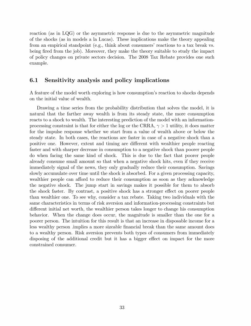
reaction (as in LQG) or the asymmetric response is due to the asymmetric magnitudeof the shocks (as in models a la Lucas). These implications make the theory appealingfrom an empirical standpoint (e.g., think about consumers�reactions to a tax break vs.being �red from the job). Moreover, they make the theory suitable to study the impactof policy changes on private sectors decision. The 2008 Tax Rebate provides one suchexample.

6.1 Sensitivity analysis and policy implications

A feature of the model worth exploring is how consumption�s reaction to shocks dependson the initial value of wealth.

Drawing a time series from the probability distribution that solves the model, it isnatural that the farther away wealth is from its steady state, the more consumptionreacts to a shock to wealth. The interesting prediction of the model with an information-processing constraint is that for either the log or the CRRA, > 1 utility, it does matterfor the impulse response whether we start from a value of wealth above or below thesteady state. In both cases, the reactions are faster in case of a negative shock than apositive one. However, extent and timing are di¤erent with wealthier people reactingfaster and with sharper decrease in consumption to a negative shock than poorer peopledo when facing the same kind of shock. This is due to the fact that poorer peoplealready consume small amount so that when a negative shock hits, even if they receiveimmediately signal of the news, they only gradually reduce their consumption. Savingsslowly accumulate over time until the shock is absorbed. For a given processing capacity,wealthier people can a¤ord to reduce their consumption as soon as they acknowledgethe negative shock. The jump start in savings makes it possible for them to absorbthe shock faster. By contrast, a positive shock has a stronger e¤ect on poorer peoplethan wealthier one. To see why, consider a tax rebate. Taking two individuals with thesame characteristics in terms of risk aversion and information-processing constraints butdi¤erent initial net worth, the wealthier person takes longer to change his consumptionbehavior. When the change does occur, the magnitude is smaller than the one for apoorer person. The intuition for this result is that an increase in disposable income for aless wealthy person .implies a more sizeable �nancial break than the same amount doesto a wealthy person. Risk aversion prevents both types of consumers from immediatelydisposing of the additional credit but it has a bigger e¤ect on impact for the moreconstrained consumer.

33

Impulse Response function as a function of wealth, �y=0:02

I II III IV V

0

2

4

6

8x 10­4

Quarters

IRF 

cons

umpt

ion

Log Util ity,κ=2.5

I II III IV V

0

2

4

6

8x 10­4

Quarters

IRF 

cons

umpt

ion

CRRA γ=5, κ=2.5

I II III IV V

0

2

4

6

8x 10­4

Quarters

IRF 

cons

umpt

ion

Log Util ity,κ=0.88

I II III IV V

0

2

4

6

8x 10­4

Quarters

IRF 

cons

umpt

ion

CRRA γ=5, κ=0.88

Figure 10. Solid: w0 = 1:94; Star Dashed:w0 = 3:3; Dotted: w0 = 5:2

34

Even in its simplicity, the model can be used to address important policy questions. Inparticular, it can be used to analyze the e¤ectiveness of tax policy reforms on individualconsumption and savings decisions. Figure 10 displays the impulse response function ofconsumption to a stimulus payment which increases income of 2% with respect to its(constant) long run level. The discretized solutions are generated using equi-spaced gridof consumption and wealth, with 50 points each. Consumption takes up value in [0:5; 3]while wealth ranges from 1 to 10. I use the same parameters (R = 1:012 and � = 1=R)of the baseline model and a simplex of size (50!) � (49) and two speci�cations of utilityfunctions. In both cases I choose � so that the capacities corresponds to �= 2:5 bits and0:88 bits28. Once the value iteration converged, I generate the impulse response functionby simulating a time series path of consumption and wealth with 10; 000Monte Carlo runsfor each initial condition on wealth. I consider three initial values of wealth as a proxy ofpopulation with low, middle and low net worth. I then average the time series per quartersand simplex points. Figure 10 gives interesting insights on the e¤ect of the stimulus onconsumer spending. For the degrees of risk aversion considered and information capacity,the reaction of the stimulus is higher the lower the initial wealth. This is not surprising, asthe stimulus payments have bigger impact on the disposable income of credit constrainedconsumers than richer people. For a given amount of information capacity and wealth,the higher the risk aversion, the lower the spending in the �rst quarter. This result alsomakes sense. If a consumer is risk averse and have no credit frictions, he allocates moreattention in processing information about low values of wealth. This leads to processinginformation slower and, in turn, reacting slower to positive news to income (Result 3).Finally for a given wealth and degree of risk aversion, the lower the information processingcapacity, the lower the response of consumption spending to the rebate. The �ndings inFigure 10 can be summarized as:

Result 4. Economic stimulus and rational inattention. The impact of a one timetax rebate on rational inattentive consumers:

1. is stronger the lower the initial net worth.

2. is more delayed the higher the degree of risk aversion.

3. is more persistent but less e¤ective the lower the information-processing capacity.

The insights one can gather from the model have strong policy implications on thee¤ectiveness of tax reform on people�s behavior. The 2008 tax rebate provides one suchexample. The model predicts that such a policy has greater response on impact forindividual with low net worth. Figure 10 also suggests that the e¤ect will be mild andspread out through several quarters for middle-high income households. These �ndingsare consistent with the empircal evidence on consumers spending of 2001 tax rebates(cfr., Johnson, Parker and Soules (2006)).

28The constraint � = 2:5 corresponds to �log = 0:01 and �crra = 0:05 for the log case and the crra, = 2 case respectively, while � = 0:88 is given by �log = 0:1 and �crra = 0:9:

35

7 Conclusions

This paper applies rational inattention to a dynamic model of consumption and savings.Consumers rationally choose the nature of the signal they want to acquire subject to thelimits of their information processing capacity. The dynamic interaction of risk aversionand endogenous choice of information �ow enhances precautionary savings.

I showed that for a given degree of risk aversion, the lower the information �ow, the�atter the consumption path. The model predicts that for a given information �ow, thehigher the degree of risk aversion, the more persistent consumption. Also, for a givendegree of risk aversion, the lower the information �ow, the more volatile consumption.

Furthermore, the model predicts that consumption path has humps. Under information-processing constraints, an hump occurs when people consume a little and save a lot whilecollecting information about wealth. When consumers realize that they are rich, they in-crease consumption and decumulate savings. This increase stops when they acknowledgethat their wealth is low again: they start to save and process more information. Thus,consumption decreases. Consistent with the previous two results, I �nd that the peak inconsumption is delayed the more the individual becomes risk averse.

Di¤ering from other life-cycle models, in my model there could be more than onehump in the consumption path. Depending on the history of the income shocks, a verylow or very high realization of income a¤ects consumers� signal through its e¤ect onwealth. Consumers react to the news by varying savings and information over time,thereby generating another hump.

Finally, the model predicts that consumers with processing capacity constraints haveasymmetric responses to shocks, with negative shocks producing more persistent e¤ectsthan positive ones. This asymmetry, observed in actual data, is novel to the theoreticalliterature of consumption and savings. Studying the reactions of rational inattentivepeople to temporary income shocks can also be used to assess the e¤ectiveness of policyreforms on consumption spending. The model predicts that, for a given level of wealth,the speed and magnitude of the consumption adjustment to the income shock depends ontheir processing capacity. Moreover, consumers with low wealth react faster to temporarytax relief than wealthier people. The results agree with both intuition and preliminarydata on consumer spending.

The results seem to suggest that enriching the standard macroeconomic toolbox withrational inattention theory is a step worth taking.

36

References

[1] Allen, F., S. Morris and H. S. Shin, (2006), Beauty Contests, Bubbles and IteratedExpectations in Asset Markets Review of Financial Studies, forthcoming.

[2] Alvarez, F. and N. Stockey, (1998), Dynamic Programming with Homogeneous Func-tions, Journal of Economic Theory, 82, pp.167-189.

[3] Amato, J.S. Morris and H. S. Shin (2002), Communication and Monetary Policy,Oxford Review of Economic Policy 18, pp. 495-503.

[4] Ameriks, J., Andrew C. and J. Leahy (2003b) The Absent-Minded Consumer, un-published, New York University.

[5] Angeletos G.-M. and A. Pavan, (2004), Transparency of Information and Coordina-tion in Economies with Investment Complementarities, American Economic Review94 (2).

[6] Aoki, K. (2003), On the Optimal Monetary Policy Response to Noisy Indicators,Journal of Monetary Economics 50, pp. 501-523.

[7] Astrom, K. (1965), Optimal Control of Markov decision process with incomplete stateestimation. Journal of Mathematical Analysis and Applications 10, pp.174-205

[8] Broda, C. and J. Parker (2008), A preliminary analysis of how household spendingchanged in response to the receipt of a 2008 economic stymulus payment. Mimeo.

[9] Caballero, R. J. (1990), Expenditure on Durable Goods: a case for slow adjustment,The Quarterly Journal of Economics, Vol. 105, No. 3. pp. 727-743.

[10] Caballero, R. J. (1995), Near-rationality, Heterogeneity and Aggregate Consumption,Journal of Money, Credit and Banking, 27 (1), pp29-48.

[11] Campbell, J.Y. (1987), Does Savings Anticipate Declining Labor Income? An alter-native Test of the Permanent Income Hypothesis, Econometrica, 55, pp.1249-1273.

[12] Campbell, J.Y. and A. Deaton (1989), Why is Consumption so Smooth? Review ofEconomic Studies, 56, pp.357-374.

[13] Campbell, J.Y. and N. G. Mankiw (1989), Consumption, Income and Interest Rates:Reinterpreting the Time Series Evidence, NBER Macroeconomic Annual 4, pp.185-216.

[14] Campbell, J.Y. and N. G. Mankiw (1989), Permanent Income, Current Income andConsumption, Journal of Business and Economic Statistics, 8 (3), pp.265-279.

[15] Carroll, C. D. (2003) Macroeconomic Expectations of Households and ProfessionalForecasters, Quarterly Journal of Economics, 118 (1), pp. 269-298.

37

[16] Cochrane, J.H. (1989), The Sensitivity of Tests of the Intertemporal Allocationof Consumption to Near-Rational Alternatives, American Economic Review, 90,pp.319-337.

[17] Cover, T.M. and J. A. Thomas, Elements of Information Theory, John Wiley &Sons, Inc., 1991

[18] Deaton, A. (1987), Life-Cycle Models of Consumption: is the evidence consistentwith the Theory? in Advances in Econometrics, Fifth World Congress, vol.2, ed.Truman Bewley, Cambridge, Cambridge University Press.

[19] Deaton, A. (1992), Understanding Consumption, Oxford, Oxford University Press.

[20] Dynan, Karen (2000), Habit Formation in Consumer Preferences: Evidence fromPanel Data, American Economic Review, 90, pp. 391-406.

[21] Flavin, M. A. (1981), The Adjustment of Consumption to Changing Expectationsabout Future Income, Journal of Political Economy, 89, pp. 974-1009.

[22] Friedman, M. (1957), A Theory of the Consumption Function, Princeton, PrincetonUniversity Press.

[23] Goodfriend, Marvin (1992), Information-Aggregation Bias, American Economic Re-view, 82, pp. 508-519.

[24] Gourinchas, P-O, and J.A. Parker (2002), Consumption over the Life-Cycle, Econo-metrica, vol. 70 (1), pp.47-89.

[25] Hall, R. (1978), Stochastic Implications of the Life Cycle-Permanent Income Hy-pothesis: Theory and Evidence, Journal of Political Economy, 86, pp.971-987.

[26] Hellwig, C. (2004), Heterogeneous Information and the Bene�ts of Transparency,Discussion paper, UCLA.

[27] Hellwig, C. and L. Veldkamp, (2006) Knowing What Others Know: CoordinationMotives in Information Acquisition, NYU, mimeo.

[28] Johnson, D., Parker, J. and N. Soules (2006) Household expenditure and the incometax rebates of 2001. American Economic Review, Vol. 96, No. 5.

[29] Kim, J., Kim, S., Schaumburg, E. and C. Sims (2005). Calculating and Using SecondOrder Accurate Solutions of Discrete Time Dynamic Equilibrium Models. mimeo.

[30] Lewis, K. (2007), The life-cycle e¤ects of information-processing constraints.Work-ing Paper, University of Iowa.

[31] Lewis, K. (2008), The Two-Period Rational Inattention Model: Accellerations andAnalyses", Computational Economics, Forthcoming. Currently available as FederalReserve Financial & Economics Discussion Series Paper, No. 2008-22, Board ofGovernors .

38

[32] Lorenzoni, G. (2006), Demand Shocks and Monetary Policy, MIT, mimeo.

[33] Lucas, R. E., J. (1973), Some International Evidence on Output-In�ation Tradeo¤s,American Economic Review, 63(3), 326�334.

[34] Luo, Y. (2007), Consumption Dynamics, Asset Pricing, and Welfare E¤ects underInformation Processing Constraints, forthcoming in Review of Dynamics.

[35] Lusardi, A.(1999), Information, Expectations, and Savings, in Behavioral Di-mensions of Retirement Economics, ed. Henry Aaron, Brookings InstitutionPress/Russell Sage Foundation, New York, pp. 81-115.

[36] Lusardi, A. (2003), Planning and Savings for Retirement, Dartmouth College, un-published.

[37] MacKay, David J. C (2003). Information Theory, Inference, and Learning Algo-rithms, Cambridge University Press, 2003

[38] Macrowiack, B., and M. Wiederholt (2007), Optimal Sticky Prices under RationalInattention, Discussion paper, Northwestern/ ECB mimeo.

[39] Mankiw, N.G. and R. Reis (2002), Sticky information versus sticky prices: A pro-posal to replace the New Keynesian Phillips curve, Quarterly Journal of Economics117, 1295�1328.

[40] Mankiw, N. G., Reis, R. and J. Wolfers (2004) Disagreement in In�ation Expecta-tions, NBER Macroeconomics Annual 2003, vol. 18, pp. 209-147.

[41] Mondria, J. (2006), Financial Contagion and Attention Allocation, Working paper,University of Toronto.

[42] Morris, S., and H. S. Shin (2002), The Social Value of Public Information, AmericanEconomic Review, 92, 1521�1534.

[43] Moscarini, G. (2004), Limited Information Capacity as a Source of Inertia, Journalof Economic Dynamics and Control, pp. 2003�2035.

[44] Mullainathan, S. (2002), A Memory-Based Model of Bounded Rationality, QuarterlyJournal of Economics, 117 (3), pp. 735-774.

[45] Orphanides, A. (2003),Monetary Policy Evaluation with Noisy Information, Journalof Monetary Economics 50 (3), pp. 605-631.

[46] Parker, J. (1999) The Reaction of Household Consumption to Predictable Changesin Social Security Taxes, American Economic Review, 89 (4), pp. 959-973.

[47] Peng, L. (2005), Learning with Information Capacity Constraints, Journal of Finan-cial and Quantitative Analysis, 40(2), 307�329.

39

[48] Peng, L., and W. Xiong (2005), Investor Attention, Overcon�dence and CategoryLearning, Discussion paper, Princeton University.

[49] Pischke, Jorn-Ste¤en (1995) Individual Income, Incomplete Information, and Aggre-gate Consumption, Econometrica, 63 (4), pp. 805-840.

[50] Puterman, M.L. (1994), Markov Decision Processes: Discrete Stochastic DynamicProgramming, Wiley Series in Probability and Mathematical Statistics, John Wileyand Sons, Inc.

[51] Reis, R. A. (2006) Inattentive Consumers, Journal of Monetary Economics, 53 (8),1761-1800.

[52] Schmitt-Grohè, S. and M. Uribe(2004). Solving Dynamic General Equilibrium Mod-els Using a Second-Order Approximation to the Policy Function. Journal of Eco-nomic Dynamics and Control 28, pp.755-75.

[53] Rotemberg, Julio J., and Michael Woodford, 1999. �The Cyclical Behavior of Pricesand Costs.� in John B. Taylor, and Michael Woodford (ed.), Handbook of Macro-economics.

[54] Shimer, Robert, 2005. �The Cyclical Behavior of Equilibrium Unemployment andVacancies.�American Economic Review. 95 (1): 25�49.

[55] Smets, Frank, and Rafael Wouters, 2003. �An Estimated Dynamic Stochastic Gen-eral Equilibrium Model of the Euro Area.�Journal of the European Economic As-sociation. 1 (5): 1123�1175.

[56] Smets, Frank, and Rafael Wouters, 2007. �Shocks and Frictions in US BusinessCycles: A Bayesian DSGE Approach.�American Economic Review. 97 (3): 586�606.

[57] Sims, C. A. (1998), Stickiness, Carnegie-rochester Conference Series On Public Pol-icy, 49(1), 317�356.

[58] Sims, C. A. (2003), Implications of Rational Inattention, Journal of Monetary Eco-nomics, 50(3), 665�690.

[59] Sims, C. A.(2005), Rational Inattention: a Research Agenda, Princeton Universitymimeo.

[60] Van Nieuwerburgh, S., and L. Veldkamp (2004a), Information Acquisition and Port-folio Under-Diversication, Discussion paper, Stern School of Business, NYU.

[61] Stokey, N. L. and R. E. Lucas Jr., with Edward C. Prescott (1989) Recursive Methodsin Economic Dynamics, Cambridge, Harvard University Press.

[62] Van Nieuwerburgh, S., and L. Veldkamp (2004b), Information Immobility and theHome Bias Puzzle, Discussion paper, Stern School of Business, NYU.

40

[63] Van Nieuwerburgh, S., and L. Veldkamp, 2006, Learning Asymmetries in Real Busi-ness Cycles, Journal of Monetary Economics 53 (4), pp.753-772.

[64] Wilson, Andrea (2003) �Bounded Memory and Biases in Information Processing,�unpublished, Princeton University.

[65] Woodford, M. (2002), Imperfect Common Knowledge and the E¤ects of MonetaryPolicy, in P. Aghion, R. Frydman, J. Stiglitz, and M. Woodford, eds., Knowledge,Information, and Expectations in Modern Macroeconomics: In Honor of Edmund S.Phelps, Princeton: Princeton University Press.

[66] Woodford, M. (2003), Interest and Prices, Princeton. Princeton University Press

[67] Zeldes, S. (1989) Optimal Consumption with Stochastic Income: Deviations fromCertainty Equivalence, Quarterly Journal of Economics, May 1989, 275-98..

41

8 Appendix A

8.1 Proof of Proposition 1.

The Bellman Recursion in the discrete Rational Inattention Consumption-Saving Model is a Contraction Mapping.

Proof. The H mapping displays:

HV (g) = maxpHpV (g) ;

with

HpV (g) =

"Xw2w

Xc2c

u (c) p (cjw)!g (w) + �

Xw2w

Xc2c

(V (g0c (�))) p (cjw) g (w)#:

Suppose that jjHV �HU jj is the maximum at point g. Let p1 denote the optimal controlfor HV under g and p2 the optimal one for HU

HV (g) = Hp1V (g) ;

HU (g) = Hp2U (g) :

Then it holdsjjHV (g)�HU (g)jj = Hp1V (g)�Hp2U (g) :

Suppose WLOG that HV (g) � HU (g) : Since p1 maximizes HV at g , I get

Hp2V (g) � Hp1V (g) :

Hence,

jjHV �HU jj =jjHV (g)�HU (g)jj =Hp1V (g)�Hp2U (g) �Hp2V (g)�Hp2U (g) =

�Xw2w

Xc2c

[(V p2 (g0c (�)))� (Up2 (g0c (�)))] p2g (w) �

�Xw2w

Xc2c

(jjV � U jj) p2g (w) �

� jjV � U jj :Recalling that 0 � � < 1 completes the proof.

42

8.2 Proof of Corollary.

The Bellman Recursion in the discrete Rational Inattention Consumption-Saving Model is an Isotonic Mapping.

Proof. Let p1 denote the optimal control for HV under g and p2 the optimal one forHU

HV (g) = Hp1V (g) ;

HU (g) = Hp2U (g) :

By de�nition,Hp1U (g) � Hp2U (g) :

From a given g, it is possible to compute g0c (�)jp1 for an arbitrary c and then the followingwill hold

V � U =)8g (w) ; c;

V�g0c (�)jp1

�� U

�g0c (�)jp1

�=)X

c2c

V�g0c (�)jp1

�� p1g �

Xc2c

U�g0c (�)jp1

�� p1g =)

Xw2w

Xc2c

u (c) p1

!g (w) + �

Xc2c

V�g0c (�)jp1

�� p1g

�Xw2w

Xc2c

u (c) p1

!=)

Hp1V (g) � Hp1U (g) =)Hp1V (g) � Hp2U (g) =)HV (g) � HU (g) =)

HV � HU:

Note that g was chosen arbitrarily and, from it, g0c (�)jp1 completes the argument that thevalue function is isotone.

8.3 Proof of Proposition 2.

The Optimal Value Function in the discrete Rational Inattention Consumption-Saving Model is Piecewise Linear and Convex (PCWL).

43

Proof. The proof is done via induction. I assume that all the operations are well-de�ned in their corresponding spaces. For planning horizon n = 0, I have only to takeinto account the immediate expected rewards and thus I have that:

V0 (g) = maxp2�

"Xw2w

Xc2c

u (c) p

!g (w)

#(24)

and therefore if I de�ne the vectors

��i0 (w)

i� Xc2c

u (c) p

!p2�

(25)

I have the desiredV0 (g) = max

f�i0(w)gi

�i0; g

�(26)

where h:; :i denotes the inner product h�i0; gi �Xw2w

�i0 (w) ; g (w). For the general case,

using equation (22):

Vn (g) = maxp2�

26664Xw2w

Xc2c

u (c) p (cjw)!g (w)+

+�Xw2w

Xc2c

(Vn�1 (g0c (�)c)) p (cjw) g (w)

37775 (27)

by the induction hypothesis

Vn�1 (g (�)jc) = maxf�in�1gi

�in�1; g

0c (�)�

(28)

Plugging into the above equation (19) and by de�nition of h:; :i ,

Vn�1 (g0c (�)) = max

f�in�1gi

Xw02w

�in�1 (w0)

Xw2w

Xc2c

T (�;w; c) Pr (w; c)Pr (c)

!(29)

With the above:

Vn (g) = maxp2�

266664Xw2w

Xc2c

u (c) p

!g (w)+

+�maxf�in�1giXw02w

�in�1 (w0)

Xw2w

Xc2c

T (�;w;c)Pr(c)

� p!g (w)

!377775

= maxp2�

"hu (c) � p; g (w)i+ �

Xc2c

1

Pr (c)maxf�in�1gi

* Xw02w

�in�1 (w0)T (�;w; c) � p; g

+#(30)

44

At this point, it is possible to de�ne

�jp;c (w) =Xw02w

�in�1 (w0)T (� : w; c) � p: (31)

Note that these hyperplanes are independent on the prior g for which I am computingVn: Thus, the value function amounts to

Vn (g) = maxp2�

"hu (c) � p; gi+ �

Xc2c

1

Pr (c)maxf�jp;cg

j

�jp;c; g

�#; (32)

and de�ne:�p;c;g = arg max

f�jp;cgj

�jp;c; g

�: (33)

Note that �p;c;g is a subset of �jp;c and using this subset results into

Vn (g) = maxp2�

"hu (c) � p; gi+ �

Xc2c

1

Pr (c)h�p;c;g; gi

#

= maxp2�

*u (c) �+�

Xc2c

1

Pr (c)�p;c;g; g

+: (34)

Now ��ini=[8g

(u (c) � p+ �

Xc2c

1

Pr (c)�p;c;g

)p2�

(35)

is a �nite set of linear function parametrized in the action set.

8.4 Proof of Proposition 3.

Proof. The �rst task is to prove that f�ingi sets are discrete for all n. The proof proceedsvia induction. Assuming CRRA utility and since the optimal policy belongs to �, it isstraightforward to see that through (25), the set of vectors f�i0gi,

��i0i� Xw2w

Xc2c

c1�

1� p (cjw)

!g (w)

!p2�

is discrete. For the general case, observe that for discrete controls and assuming M =����jn�1��, the sets ��jp;c are discrete, for a given action p and consumption c, I can onlygenerate �jp;c�vectors. Now, �xing p it is possible to select one of theM �jp;c�vectors foreach one of the observed consumption c and, thus, f�jngi is a discrete set. The previousproposition, shows the value function to be convex. The piecewise-linear component ofthe properties comes from the fact that f�jngi set is of �nite cardinality. It follows thatVn is de�ned as a �nite set of linear functions.

45

9 Appendix B

9.1 Concavity of Mutual information in the Belief State.

For a given p (cjw),Mutual Information is concave in g (w)

Proof. Let Z be the binary random variable with P (Z = 0) = � and let W = W1 ifZ = 0 and W = W2 if Z = 1. Consider

I (W;Z;C) = I (W ;C) + I (Z;CjW )= I (W ;CjZ) + I (Z;C)

Condition on W , C and Z are independent, I (C;ZjW ) = 0: Thus,

I (W ;C) � I (W ;CjZ)= � (I (W ;CjZ = 0)) + (1� �) (I (W ;CjZ = 1))= � (I (W1;C)) + (1� �) (I (W2;C))

Q.E.D.

10 Appendix C

Pseudocode

Let � be the shadow cost associated to �t = It (Ct;Wt). De�ne a Model as a pair ( ; �).For a given speci�cation :

� Step 1: Build the simplex. Construct an equi-spaced grid to approximate each g (wt)-simplex point.

� Step 2: For each simplex point, de�ne p (ct; wt). and Initialize with V�g0cj (�)

�= 0:

� Step 3: For each simplex point, �nd p� (c; w) s.t.

V0 (g (wt))jp�(ct;wt) = maxp(ct;wt)� Pwt2w

Pct2c

�c1� t

1�

�p� (ct; wt)� � [It (Ct;Wt)]

�:

� Step 4: For each simplex point, compute g0cj (�) =P

wt2w T (�;wt; ct) p� (wtjct). Use a

kernel regression to interpolate V0 (g (wt)) into g0cj (�).

� Step 5: Optimize using csminwel and iterate on the value function up to convergence.

46

Obs. Convergence and Computation Time vary with the speci�cation ( ; �).

! 180-320 iterations each taking 8min-20min

� Step 6. For each model ( ; �), draw from the ergodic p� (c; w) a sample (ct; wt) andsimulate the time series of consumption, wealth, expected wealth and information �owby averaging over 1000 draws.

� Step 7. Generate histograms of consumption and impulse response function of consump-tion to temporary positive and negative shocks to income.

11 Appendix D

11.1 Optimality Conditions

In this section I incorporate explicitly the constraint on information processing and derivethe Euler Equations that characterize its solution.

The main feature of this section is to relate the link between the output of the channelconsumption, with the capacity chosen by the agent. In deriving the optimality condi-tions, I incorporate the consistency assumption (20) in the main diagonal of the jointdistribution to be chosen, Pr t (cj; wi). Note that such a restriction is WLOG. I thenshow the analytical details of the derivatives with respect to control and states.

11.2 First Order Conditions

To evaluate the derivative of the Bellman equation with respect to a generic distrib-ution Pr (ck1 ; wk2), de�ne the di¤erential operator �kv (l) � v (lk1) � v (lk2) and � asthe shadow cost of processing information: Then, the optimal control for the program(17)-(21) amounts to:

@p� (ck1 ; wk2) :

�ku (c) + ��kV (g0c (:)) = p� (ck1 ; wk2)

���ku

0 (c) �p� (wk2jck1)� ��kV0p� (g

0c (:))

�(36)

This expression states that the optimal distribution depends on the weighted di¤er-ence of two consumption pro�les, ck1 and ck2 where the weights are given by current andfuture discounted utilities. Note that the di¤erential of the marginal utility of currentconsumption is also weighted by the conditional optimal distribution of consumption andwealth.

The interpretation of (36) is that the optimal probability of consumption and wealthdepends on both levels of current and intertemporal utility and marginal utility. In

47

particular, there is an intertemporal trade-o¤by consuming the maximum value of wealthallowed by the signal, ck2 and a lower consumption ck2. To illustrate the argument,suppose a consumer believes that his wealth is wk2 with high probability. Suppose forsimplicity that wk2 allows him to spend ck1 or ck2. The decision of shifting probabilityfrom p (ck2 ; wk2) to p (ck1 ; wk2) depends on four variables. First, the current di¤erencein utility levels, �ku (c) which tells the immediate satisfaction of consuming ck1 ratherthan ck2. However, consuming more today has a cost in future consumption and wealthlevels tomorrow, ��kV (g

0c (:)). Optimal allocation of probabilities requires trading o¤

not only intertemporal levels of utility but also marginal intertemporal utilities wherenow the current marginal utility of consumption is weighted by the e¤ort required toprocess information today.

To explore this relation further, I evaluate the derivative of the continuation value fora given optimal p� (ck1 ; wk2), that is �kV

0p� (g

0c (:)). To this end, de�ne the ratio between

di¤erential in utilities (current and discounted future) and di¤erential in marginal currentutility as � � �ku(c(�))+��kV (g

0c(:))

��[u0(ck1 (�))�u0(ck2 (�))]. Also, let �� be the ratio � when current level of

utilities are equalized and future di¤erential utilities are constant, i.e., �ku (c) = 0 and�kV (g

0c (:)) = 1 or, �

� � �

��[u0(ck1 (�))�u0(ck2 (�))]. Then, an application of Chain rule and

point-wise di¤erentiation leads to

p� (ck1 ; wk2) = � (k1; k2) p� (ck1) (37)

where

� (k1; k2) � �1 (�; p� (ck1 ; wk2))��2���; g0ck1

(�) ; p� (ck1 ; wk2)���3���; g0ck2

(�) ; p� (ck1 ; wk2)�

Let me focus on the explanation for the terms � (k1; k2) which characterize the optimalsolution of the conditional distribution p� (wk2 jck1) :

The �rst term �1 (�; p� (ck1 ; wk2)) � exp (�= (p� (ck1 ; wk2))) states that the optimalchoice of the distribution balances di¤erentials between current and future levels of utili-ties between high (k2) and low (k1) values of consumption. In case of log utility, the termexp (�) is a likelihood ratio between utilities in the two states of the word (k1 and k2) andthe interpretation is that the higher is the value of the state of the world k2 with respectto k1 as measured by the utility of consumption, the lower is the optimal p� (ck1 ; wk2).This matches the intuition because the consumer would like to place more probabilityon the occurrence of k2 the wider the di¤erence between ck1 and ck2. A perhaps moreinteresting intertemporal relation is captured by the terms �2 and �3, both of whichdisplay the occurrence of the update distribution g0cki (�), i = 1; 2. To disentangle thecontribution of each argument of �2 and �3, I combine the derivative of the control withthe envelope condition. Let �01 be the term �1 led one period and de�ne the di¤erentialbetween transition from one particular state to another and transition from one particu-

lar state to all the possible states as ~�Tj � T��;wk2 ; ckj

���P

i

T (�;wi; ck1) p��wijckj

��for j = 1; 2. Evaluating the derivative with respect to the state almost surely reveals

48

that �2 � exp������01

~�T1

�=p (ck1)

�while �3 � exp

������01

~�T2=p (ck2)��. The

terms �2 and �3 reveal that in setting the optimal distribution p� (ck1 ; wk2) consumerstake into account not only di¤erential between levels and marginal utilities but also howthe choice of the distribution shrinks or widens the spectrum of states that are reachableafter observing the realized consumption pro�le.

An interesting special case that admits a closed form solution is when the agent isrisk neutral. Consider the framework in Section (3.2) and let utility take up the formu (c) = ct, then in the region of admissible solution ct < wt, the optimal probabilitydistribution makes c independent on w. To see this, it is easy to check that in the twoperiod case with no discounting, the utility function reduces to u (c) = w, which impliescjw / U (wmin; wmax). That is, since all the uncertainty is driven by w, the consumer doesnot bother processing information beyond the knowledge of where the limit of c = w lies.In other word, the constraint on information �ow does not bind. With the continuationvalue, exploiting risk neutrality, the optimal policy function amounts to:

p� (wk2jck1) =e

[(ck1�ck2)+��k �V (g

0c(:))]

�

!Pj

~�Tj(38)

The solution uncovers some important properties of the interplay between risk neutralityand information �ow. First of all, households with linear utility do not spend extraconsumption units in sharpening their knowledge of wealth. This is due to the fact thatbecause the consumer is risk neutral and, at the margin, costs and bene�ts of information�ows are equalized amongst periods, there is no necessity to gather more informationthan the boundaries of current consumption possibilities. In each period, the presence ofinformation processing constraint forces the consumer to allocate some utils to learn justenough to prevent violating the non-borrowing constraint. Once those limits are �guredout, the consumption pro�les in the region c < w are independent on the value of wealth.

Derivative with Respect to Controls In the main text, I state that the optimalcontrol amounts to :

@p� (ck1 ; wk2) :

�ku (c (�)) + ��kV (g0c (:)) = p� (ck1 ; wk2) (���ku

0 (c (�)) + ��kVp� (g0c (:))) (39)

which can be rewritten, opening up the operator �k as:

'�(ck1 ;ck2)= Pr (ck1 ; wk2)

0@ �(ck1 ;ck2 ;�) ln Pr (ck1 ; wk2)Pr (ck1)+ �

24@V 0�g0ck1

(�)�

@ Pr (ck1 ; wk2)�@V 0

�g0ck2

(�)�

@ Pr (ck1 ; wk2)

351Awhere

49

� '�(ck1 ;ck2)

� �hu (ck1 (�))� u (ck2 (�)) + �

�V�g0ck1

(�)�� V

�g0ck2

(�)��i

, and

� �(ck1 ;ck2 ;�)� �� [u0 (ck1 (�))� u0 (ck2 (�))] :

Note that by Chain rule@V 0

�g0ckj

(�)�

@ Pr(ckj ;wk2)=

@V 0�g0ckj

(�)�

@

�g0ckj

(�)� @

�g0ckj

(�)�

@ Pr(ckj ;wk2), for j = 1; 2: Plug (36)

in the second term of the above expression and evaluating point-wise the derivativesdelivers

In cj = ck1 ;

=)@g

��jck1

�@ Pr(ck1 ;wk2)

=@

"1

p(ck1)

Pi

T(�;wi;ck1)Pr(wi;ck1)!#

@ Pr(ck1 ;wk2)=

1

p (ck1)

0BB@T (�;wk2 ; ck1)��P

i

T (�;wi; ck1) Pr (wi; ck1)�

p (ck1)

1CCADe�ne � �

'�

(ck1 ;ck2) �

(ck1 ;ck2)and �� � �

�

(ck1 ;ck2 ;�); to get rid of cumbersome notation, let

(k1; k2) ���;��; g0ck1

(�) ; g0ck2 (�) ;Pr (ck1 ; wk2) ;�: Then the �rst order conditions

result intoPr (ck1 ; wk2) = � (k1; k2) Pr (ck1) (40)

where

� (k1; k2) � �1 (�;Pr (ck1 ; wk2))��2���; g0ck1

(�) ;Pr (ck1 ; wk2)���3���; g0ck2

(�) ;Pr (ck1 ; wk2)�

while

� �1 (�;Pr (ck1 ; wk2)) � e

0B@� 1

Pr(ck1 ;wk2)

1CA;

� �2���; g0ck1

(�) ;Pr (ck1 ; wk2)�� e

0BBB@��� @V�g0ck1

(�)�

@

�g0ck1

(�)� 1

p(ck1)

0BBB@T(�;wk2 ;ck1)�0@P

i

T(�;wi;ck1)Pr(wi;ck1)1A

p(ck1)

1CCCA1CCCA;

� �3 (k1; k2) � e

0BBB@�� @V�g0ck2

(�)�

@

�g0ck2

(�)� 1

p(ck2)

0BBB@T(�;wk2 ;ck2)�0@P

i

T(�;wi;ck1)Pr(wi;ck2)1A

p(ck2)

1CCCA1CCCA:

50

Derivative with Respect to States To derive the envelope condition with respectto a generic state g (wk) for k = 1; 2; 3, let me start by placing the restrictions on themarginal distribution of wealth in the main diagonal of the joint distribution Pr (c; w).The derivative then amounts to:

@ Pr t(cj ;wk)

@g(wk)=

@ Pr t(cj)

@g(wk)=

8<:1 f(j = k) \ (j 6= max l 2 c)g�1 fj = max l 2 cg0 o/whise

:

Let lmax denote the maximum indicator l belonging to c: Then the derivative of thestate g (wk) displays:

@V (g(wk))@g(wk)

a:s=�

u (ck (�)) + ��V�g0ck (�)

����u�clmax

(�)�+ �V

�g0clmax

(�)���

+

���log�Pr(ck;wk)p(ck)g(wk)

�u0 (ck (�)) Pr (ck; wk)� log

�Pr(clmax ;wk)p(clmax )g(wk)

�u0�clmax (�)

�Pr�clmax ; wk

��+

+�P

j

"@V

�g0ckj

(�)�

@

�g0ckj

(�)� @

�g0ckj

(�)�

@g(wk)

!Pr (cj; wk)

#:

Combining �rst order conditions and the envelope condition after some algebra leadsto the result in (40).

12 Appendix E.

12.1 A simple example

To illustrate how a consumer with information constraints di¤ers from a consumer withfull information and a consumer with no information, consider the following model ofconsumer�s choice.

Suppose the household has three wealth possibilities, w 2 W � f2; 4; 6g, and threeconsumption possibilities c 2 C � f2; 4; 6g. Before any observation is made, the con-sumer has the following prior on wealth, Pr (w = 2) = :5, Pr (w = 4) = :25, Pr (w = 6) =:25. Moreover the consumer cannot borrow, c � w and, if his check bounces he su¤ersc = 0. He derives utility from consumption de�ned as u (c) � log (c). His payo¤ matrixis summarized in Figure a.

cnw 2 4 6

2 0:7 0:7 0:74 �1 1:38 1:386 �1 �1 1:8

Figure a: Payo¤ Matrix with u(c)�log(c)

51

If uncertainty in the payo¤ can be reduced at no cost, the consumer would set c = w;8c 2 C; 8w 2 W .

In contrast, if he cannot gather any information about wealth besides that providedby the prior, the consumer will avoid unpleasant surprises by setting c = 2 whatever thewealth.

The di¤erence in bits in the two policies is measured by the mutual informationbetween C and W . The ex-ante uncertainty embedded in the prior for w is calculatedby evaluating its entropy in bits, i.e.,

H (W ) � �Xw2W

p (w)�log2 (p (w)) = 0:5�log2�1

0:5

�+0:25�log2

�1

0:25

�+0:25�log2

�1

0:25

�= 1:5

bits. Since observation of c provides information on wealth, conditional on the knowledgeof consumption uncertainty aboutw is reduced by the amountH (W jC) �

Xw2W

Xc2C

p (c; w) log2 (p (wj c)).

The mutual information between C and W , i.e., the remaining uncertainty about thewealth after observing consumption, is the di¤erence between ex-ante uncertainty of W(H (W )) and the knowledge of W given by C (H (W jC)). In formulae, the mutual infor-mation or capacity of the channel amounts to:

I (C;W ) =Xw2W

Xc2C

p (c; w) log

�p (c; w)

p (c) p (w)

�

To see what this formula implies, consider �rst the situation in which information can�ow at in�nite rate. In this case ex-post uncertainty is fully resolved. Moreover, notethat (p (wj c)) = 1; 8c 2 C; 8w 2 W since the consumer is setting positive probabilityon one and only one value of consumption per value of wealth. This in turns impliesH (W jC) = 0, so the mutual information in this case will be I (C;W ) = H (W ) = 1:5:bits.

Instead, if the consumer has zero information �ow or, equivalently, if processing in-formation is prohibitively hard for him, his optimal policy of setting c = 2 at all timesmakes consumption and wealth independent of each other. This implies that H (W jC) =Xw2W

Xc2C

p (c) p (w) log2

�p(c)p(w)p(c)

�!= H (W ). Hence, in this case I (C;W ) = 0 and no

reduction in the uncertainty about wealth occurs upon observing consumption. The in-tuition is that if a consumer decides to spend the same amount in consumption regardlessof his wealth level, his purchase will tell him nothing about his �nancial possibilities. Theexpected utility in the �rst case is EFullInfo (u (c)) = (log (2)) � (:5) + (log (4) + log (6)) �(:25) = 1:14 while in the second case ENoInfo (u (c)) = 0:7.

Now, assume that the consumer can allocate some e¤ort in choosing size and scopeof information about his wealth he wants to process, under the limits imposed by hisprocessing capacity. Let �� = 0:3 be the maximum amount of information �ow that the

52

consumer can process. Let the probability matrix of the consumer be:

cnw P (w = 2) P (w = 5) P (w = 8)

P (c = 2) 0:5 p1 p2P (c = 4) 0 :25� p1 p3P (c = 6) 0 0 :25� p2 � p3

Figure b: Probability Matrix

where the zeroes on the lower left corner of the matrix encode a non-borrowing constraintc � w.29 The program of the consumer is:30

maxfp1;p2;p3g

E� (u (c))

s.t.�� � I (C;W ) :

Given �� = 0:3,31 the optimal policy sets p�1 = 0:125; p�2 = 0:125, p3 = 0:125, whichcorresponds to Pr (C = 2) = 0:75; Pr (C = 4) = 0:25, Pr (C = 6) = 0. This leads to anexpected utility of E� (u (c)) = 0:87. Hence, consumers who invest e¤ort in tracking theirwealth using the channel are better o¤ than in the no information case (higher expectedutility) even though they cannot do as well as in the constrained case.

Note that the result of trading information for the highest value to gain a more preciseknowledge of the lower value of wealth is driven by the functional form of utility. For

29I append a non-borrowing constraint c � w to reduce the number of the probabilities to be calculatedin Figure (b), thereby keeping the example easy. Figure (b) can be rationalized by assuming that theconsumer acquires a signal on wealth ws = w+ " and chooses the distribution of " always such that thesupport of " is in (0;�1]. One can think that �� is net of the bits used to set the desired support of ".30In details:

maxfp1;p2;p3g

E� (u (c)) = (log (2)) � (:5 + p1 + p2) +

+ (log (4)) � (:25� p1 + p3) ++ (log (6)) � (:25� p2 � p3)

and

�� � I (C;W ) =

= :5 log2

�:5

:5 (:5 + p1 + p2)

�+ :p1 log2

�p1

:25 (:5 + p1 + p2)

�+

+p2 log2

�p2

:25 (:5 + p1 + p2)

�+ (:25� p1) log2

�(:25� p1)

:25 (:25� p1 + p3)

�+

+(:25� p2 � p3) log2�

(:25� p2 � p3):25 (:25� p2 � p3)

�:

31Note that such a bound of information �ow is unrealistically low. However I decided to trade o¤realism for simplicity in this example.

53

instance, a consumer with the same bound on processing capacity but CRRA utility withcoe¢ cient of risk aversion, say, = 5, would have chosen a probability Pr (C = 2) lowerthan his log-utility counterpart. This is because higher degrees of risk aversion induce theconsumers to be better informed about low values of wealth to avoid such occurrences.The intuition is that because the attention of the consumer within the limits of theShannon capacity is allocated according to his utility, the degree of risk aversion plays animportant role in determining what events receive the consumer�s attention. A log-utilityconsumer wants to be well informed about the middle values of his wealth, while a highrisk averse consumer selects a signal which provides sharper information about the lowervalues of wealth, so that he can avoid high disutility. The opposite direction is taken bythe less risk-averse agent.

12.2 Analytical Results for a three-point distribution

In this section I will focus on the optimality conditions derived above for a three pointdistribution. The goal is to fully characterize the solution for this particular case andexplore its insights.32

Let me assume the wealth to be a random variable that takes up values in w 2w � fw1; w2; w3g with distribution g (wi) = Pr (w = wi) described by:

W wl wm wh

g (wi) g1 g2 1� g1 � g2

The equation describing the evolution of the wealth is displayed by the budget constraint

wt+1 = R (wt � ct) + Yt

where I denote by Yt the exogenous stochastic income process earned by the householdand by R > 0 the (constant) interest rate on savings, (wt � ct). Like wealth, beforeprocessing information consumption, ct; is a random variable. It takes up a discretenumber of values in the event space c � fc1; c2; c3g. The joint distribution of wealthand consumption, Pr t (cj; wi), amounts to:

Pr t (cj; wi)

CnW w1 w2 w3

c1 x1 x2 x3c2 0 x4 x5c3 0 0 x6

32A three-point distribution is indeed a special case of the more general N points distribution since twoof the states in the event space w are absorbing states. This, in turn, sets to zero several dimensions ofthe problem and allows for a close form solution of the optimal policies. Although the solution for thisparticular case does not have a straightforward generalization, it provides useful insights on the optimalchoice for the joint probability distribution of wealth and consumption and its relation with the priordistribution of wealth (g (w)) and the utility of the consumer.

54

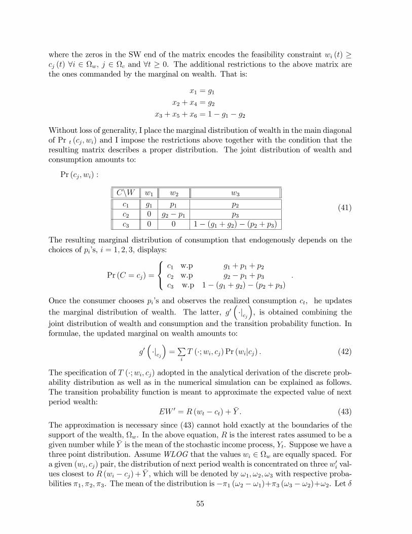
where the zeros in the SW end of the matrix encodes the feasibility constraint wi (t) �cj (t) 8i 2 w; j 2 c and 8t � 0. The additional restrictions to the above matrix arethe ones commanded by the marginal on wealth. That is:

x1 = g1

x2 + x4 = g2

x3 + x5 + x6 = 1� g1 � g2

Without loss of generality, I place the marginal distribution of wealth in the main diagonalof Pr t (cj; wi) and I impose the restrictions above together with the condition that theresulting matrix describes a proper distribution. The joint distribution of wealth andconsumption amounts to:

Pr (cj; wi) :

CnW w1 w2 w3

c1 g1 p1 p2c2 0 g2 � p1 p3c3 0 0 1� (g1 + g2)� (p2 + p3)

(41)

The resulting marginal distribution of consumption that endogenously depends on thechoices of pi�s, i = 1; 2; 3; displays:

Pr (C = cj) =

8<:c1 w.p g1 + p1 + p2c2 w.p g2 � p1 + p3c3 w.p 1� (g1 + g2)� (p2 + p3)

:

Once the consumer chooses pi�s and observes the realized consumption ct, he updatesthe marginal distribution of wealth. The latter, g0

��jcj�, is obtained combining the

joint distribution of wealth and consumption and the transition probability function. Informulae, the updated marginal on wealth amounts to:

g0��jcj�=Pi

T (�;wi; cj) Pr (wijcj) : (42)

The speci�cation of T (�;wi; cj) adopted in the analytical derivation of the discrete prob-ability distribution as well as in the numerical simulation can be explained as follows.The transition probability function is meant to approximate the expected value of nextperiod wealth:

EW 0 = R (wt � ct) + �Y : (43)

The approximation is necessary since (43) cannot hold exactly at the boundaries of thesupport of the wealth, w. In the above equation, R is the interest rates assumed to be agiven number while �Y is the mean of the stochastic income process, Yt. Suppose we have athree point distribution. AssumeWLOG that the values wi 2 w are equally spaced. Fora given (wi; cj) pair, the distribution of next period wealth is concentrated on three w0i val-ues closest to R (wi � cj)+ �Y , which will be denoted by !1; !2; !3 with respective proba-bilities �1; �2; �3. The mean of the distribution is ��1 (!2 � !1)+�3 (!3 � !2)+!2. Let �

55

be the distance between the values of wi: Then the mean becomes �! � �� (�3 � �1)+!2.The variance of the distribution is then �2! � �2 (�3 � �1) � (�! � !2)

2. Since �2 is anexact function of �1 and �3, the equations for mean and variance of the process consti-tutes two equations in two unknowns. With the additional restriction that all the �i�sare positive and sum to one, it is not possible to guarantee the existence of a solution forR (wi � cj) + �Y close to the boundaries of the support of the distribution of wealth. Tomake sure that there is always a solution for �! 2 (min (w) + :5�;max (w)� :5�), andthe solution is continuous at points where �! =

(wi+wi+1)2

, one has to choose �2! = :25�2.

Euler Equations. Making use of the marginal distribution of wealth described aboveand making use of (42) together with the speci�cations of T (�;wi; cj) and Pr (wi; cj), Ican explicitly evaluate g0

��jcj�point-wise. To illustrate this point, using the numerical

values of T (�;wi; cj) above, the derivatives point-wise are as follows.

In cj = c1;

g0��jc1�=

1

(g1 + p1 + p2)(T (�;w1; c1) g1 + T (�;w2; c1) p1 + T (�;w3; c1) p2)

In cj = c2

g0��jc2�=

1

(g2 � p1 + p3)(T (�;w2; c2) (g2 � p1) + T (�;w3; c2) p3)

In cj = c3g0��jc3�= T (�;w3; c3)

Then, the �rst order conditions and envelope conditions amount to

@p1 : �u (c1)� u (c2) + �

�V 0 �g0c2 (�)�� V 0 �g0c2 (�)���

= p1

0@ � ([u0 (c1 � ��)� u0 (c2 � ��)]) ln�

p1(g1+p1+p2)

�+

+@V 0(g0c1 (�))@g0c1 (�)

@g0c1 (�)@p1

� @V 0(g0c2 (�))@g0c2 (�)

@g0c2 (�)@p1

1ANote that

@g0cj (�)@pj

= 0 for j 2 f1; 2; 3g.33 This result is not driven by the speci�ca-tion chosen for the transition function T (�;wi; cj), but it is a feature of the three point

33To see this, plug (42) in@g0cj

(�)@pj

for j 2 f1; 2g and evaluating pointwise the derivatives delivers@g0��jc1�:

1

(g1 + p1 + p2)2

24 0:81p2 � 0:15g1� (0:56p2 � 0:15g1)

�0:25p2

35 = 0@g0��jc2�:

p3

(g2 � p1 + p3)2

24 �0:150:150

35 = 0

56

distribution. Indeed, because two of the three values of wealth are at the boundariesof w, the absorbing states w1 and w3 place tight restrictions on the continuation valueV 0�g0cj (�)

�through the transition function and, as a result, the update for the marginal

g0cj (�) according to (42). That is, the marginal probability on wealth g0cj(�) in this case

tends to its ergodic value �gcj (�). It follows that V 0 ��gcj (�)� a:s:�! �V � ��gcj (�)� which is aconstant since the functional argument is. This is what makes the 3-point distributiontractable.

For the general case, the �rst order condition with respect to the �rst control amountsto:

@p1 : �u (c1 (�))� u (c2 (�)) + �

��V (�gc1 (�))� �V (�gc2 (�))

��= p1

�� ([u0 (c1 (�))� u0 (c2 (�))]) ln

�p1

(g1 + p1 + p2)

��(44)

Similarly, for the second control

@p2 : �u (c1 (�))� u (c3 (�)) + �

��V (�gc1 (�))� �V (�gc3 (�))

��= p2

�� ([u0 (c1 (�))� u0 (c3 (�))]) ln

�p2

(g1 + p1 + p2)

��(45)

And �nally:

@p3 : �u (c2 (�))� u (c3 (�)) + �

��V (�gc2 (�))� �V (�gc3 (�))

��= p3

�� (u0 (c2 (�))� u0 (c3 (�))) ln

�p3

(g2 � p1 + p3)

��(46)

Using the result that the value function converges to V � when the utility function belongsto the family of constant absolute risk aversion (CARA), I assume the utility takes upthe speci�cation:

u (cj (�)) =

8><>:� e

� (cj(�))

for > 0

log (cj (�)) for lim !0

�� e

� (cj(�))

�where is the coe¢ cient of absolute risk aversion and j 2 c � fc1; c2; c3g. Moreover,by proposition 1, the value function is PCWL, that is:

�V��gcj (�)

�= arg max

f�0jgj

D�0j; �g

0cj(�)E

57

where��0jjare a set of vectors each of them generated for a particular observation of

previous values of consumption cj and h:; :i denotes the inner productD�0j; �g

0cj(�)E�X

w02w

�0j (w0)T (� : w; cj) � p (cjjw). To get a close form solution, I need to represent the

probability distribution of the prior. One of the possibilities is to use a particle basedrepresentation. The latter is performed by using N random samples, or particles, atpoints wi and with weights $i. The prior is then

gt (w) =NPi=1

$i~� (w � wi)

where ~� (w � wi) = Dirac (w � wi) is the Dirac delta function with the center in zero. Aparticle-based representation can approximate arbitrary probability distributions (withan in�nite number of particles in the extreme case), it can accommodate nonlinear tran-sition models without the need of linearizing the model, and it allows several quantities ofinterest to be computed e¢ ciently. In particular, the expected value in the belief updateequation becomes:

�g0��jcj�= Pr (cjj�)

NPi=1

$iT (�;wi; cj)

The central issue in the particle �lter approach is how to obtain a set of particles toapproximate �g0

��jcj�from the set of particles approximating g (w). The usual Sampling

Importance Re-sampling (SIR) approach (Dellaert et al., 1999; Isard and Blake, 1998)samples particles using the motion model T (�;wi; cj), then it assigns a new weights inorder to make all particles weights equal. The trouble with the SIR approach is that itrequires many particles to converge when the likelihood Pr (cjj�) is too peaked or whenthere is a small overlap between prior and posterior likelihood. The main problem withSIR is that it requires many particles to converge when the likelihood is too peaked orwhen there is only a small overlap between the prior and the likelihood. In the auxiliaryparticle �lter, the sampling problem is addressed by inserting the likelihood inside themixture

�g0��jcj�/

NXi=1

$i Pr (cjj�)T (�;wi; cj) :

The state (�) used to de�ne the likelihood Pr (cjj�) is not observed when the particles areresampled and this calls for the following approximation

�g0��jcj�/

NXi=1

$i Pr�cjj�i!

�T (�;wi; cj)

with �i! any likely value associated with the ith component of the transition densityT (�;wi; cj),

e.g., its mean. In this case, we have that �i! = wi + �(cj) : Then, �g0��jcj�can be re-

garded as a mixture of N transition components T (�;wi; cj) with weights $i Pr (cjj�i!) :Therefore, sampling a new particle w0j to approximate �g

0��jcj�can be carried out by

58

selecting one of the N components, say im, with probability $i � Pr (cjj�i!) and thensampling w0i from the corresponding component T (�;wim ; cj) : Sampling is performed inthe intersection of the prior and the likelihood and, consequently, particles with largerprior and larger likelihood (even if this likelihood is small in absolute value) are morelikely to be used. After the set of states for the new particles is obtained using the aboveprocedure, it is necessary to de�ne the weights. This is done using

$0m /

Pr (cjjw0m)Pr (cjj�im! )

:

Using the sample-based belief representation the averaging operator h:; :i can be com-puted in close form as:

h�; �g0i =Xw2w

"Xk

$k� (wjwk;�k)#"X

l

$0l~� (w � wl)

#

=Xk

$k

Xw2w

� (wjwk;�k)

"Xl

$l~� (w � wl)

#!=Xk

$k

Xl

$l� (wljwk;�k)

=Xk;l

$k$l� (wljwk;�k) :

where � (:) is the distribution of the r.v. W 0 that use the speci�cation of the transitionfunction above, i.e., mean �! � �� (�3 � �1) + !2 and variance �2! � �2 (�3 � �1) �(�! � !2)

2 with � the (constant) distance between the values of wi.

Representing priors in this fashion allows an explicit evaluation of the di¤erences in thevalue functions in the �rst order conditions, since V 0

��g0cj (�)

�= argmaxf�0jgj

D�0j; �g

0cj(�)E=X

k;l

~$0k ~$

0l� (wljwk;�k), where ~$0

k ��Pr(cj jw0k)Pr(cj j�k!)

�; ~$0

l ��Pr(cj jw0l)Pr(cj j�l!)

�: Since the result of

the argmax is just one of the member of the set��0jjand all the elements involved in

the de�nition of �0j function in �(p) are a �nite set of linear function parametrized in theaction set, so is the �nal result.

Let a prime (" 0 ") denote the variables led one period ahead, algebraic manipulationdelivers the following optimal control functions:

p�1 (~g; �) =g1 ( 1 � ���1)

�g1 (LambertW (�1)x12 � LambertW (�11)x11) + 2g1 ( 1 � ��v1); (47)

p�2 (~g; �) =g1 ( 2 � ���2)

�g1 (LambertW (�2)x21 � LambertW (�2)x22) + 2 2g1 ( 2 � ���3); (48)

59

p�3 (~g) = 3 � ��v3

�x3 LambertW (�3)(49)

where

� 1 ��e� (c2���)e� (c1���)

�; 2 �

�e� (c3���)e� (c1���)

�; 3 �

�e� (c3���)e� (c2���)

�;

� �1 � g2 ( 03) + (g2 � g1) (

02 � 03) ;

� �2 � g2 ( 01) + (g2 � g1) (

01 � 02) ;

� �3 � (1� g2 � g1) ( 02) + (g2 � g1) (

03 � 01)

� �1 �( 1���v1) 1�g1(e (c2�c1))

; ; x11 � e� (c1���); x12 � e� (c2���);

� �21 �( 2���v2) 2�g1(e (c3�c1))

; x21 � e� (c1���); x22 � e� (c3���) and

� �3 � 3���v3

�g2(e (c3�c2)); x3 � e (c3�c2):

and LambertW (:) is the LambertW function that satis�es LambertW (x) eLambertW(x) =x34. The argument of the LambertW is always positive for the �rst order conditionsderived, implying that for each of the optimal policies the function returns a real solu-tion amongst other complex roots, which is unique and positive. Since @ LambertW(x)

@x=

LambertW(x)x(1+LambertW(x))

it is possible to calculate the derivatives of the above expression withrespect to f�; g1; g2g. However, the sign of the derivatives with respect to those variablesis indeterminate. The rationale behind this result is quite simple. Consider the jointprobability distribution Pr (ci; wj) . The overall e¤ect of an increase in this probabilityresults from the interplay of several factors. In general, if � is low (or, equivalently,the capacity of the channel, ��, in (18) is high), a risk averse consumer will try to re-duce the o¤ diagonal term of the joint as much as possible. That is, he would set

34Formally, the LambertW function is the inverse of the function f : C ! C given by f (x) � xex:Hence LambertW (x) is the complex function that satis�es

LambertW (x) eLambertW(x) = x

for all x 2 C:. In practice the de�nition of LambertW requires a branch cut, which is usually takenalong the negative real axis. LambertW (x) function is sometimes also called product log function.This function allows to solve the functional equation

g (x)g(x)

= x

given thatg (x) = eLambertW(ln(x)):

See Corless, Gonnet, Hare, Je rey and Knuth (1996).

60

p1 = Pr (c1; w2) ; p2 = Pr (c1; w3) and p3 = Pr (c3; w2) as low as its capacity allows himto sharpen his knowledge of the state. On the opposite extreme, for very high value ofthe cost associated to information processing, �, p1 and p2 will be higher, the higher theprior g1 = g (w1) with respect to g2 = g (w2) and g3 = g (w3). This is due to the factthat when the capacity of the channel is low -or, equivalently, the e¤ort of processinginformation is high-, the �rst order conditions indicate that it is optimal for the con-sumer to shift probabilities towards the higher belief state. The intuition is that whenit is costly to process information, the household cannot reduce the uncertainty abouthis wealth. If the individual is risk adverse as implied by the CRRA utility function, ineach period, he would rather specialize in the consumption associated to the higher priorthan attempt to consume a di¤erent quantity and running out of wealth in the followingperiods. This intuition leads to an optimal policy of the consumer that commands highprobability to one particular consumption pro�le and set the remaining probabilities aslow as possible. To illustrate this, consider a consumer who has a high value of � anda prior on w1 higher than the other priors. If he cannot sharpen his knowledge of thewealth due to prohibitively information processing e¤ort, he will optimize its dynamicproblem by placing very high probability on Pr (c1) = g1 + p1 + p2, i.e., increase p1 andp2 and decrease p3. Likewise, if g2 is higher than the other priors and � is high -� is low-,optimality commands to decrease both p1 and p2 and increase p3.

13 Appendix F:

13.1 The Mathematics of Rational Inattention

This part addresses the mathematical foundations of rational inattention. The mainreference is the seminal work of Shannon (1948). Drawing from the information theoryliterature, I provide an overview Shannon�s axiomatic characterization of entropy andmutual information and show the main theoretical features of these two quantities.

Formally, the starting point is a set of possible events whose probabilities of occurrenceare p1; p2; : : : ; pn. Suppose for a moment that these probabilities are known but that isall we know concerning which event will occur. The quantity H = �

Pi pi log pi is called

the entropy of the set of probabilities p1; : : : ; pn. If x is a chance variable, then H (x)indicates its entropy; thus x is not an argument of a function but a label for a number,to di¤erentiate it from H (y) say, the entropy of the chance variable y.

Quantities of the form H = �P

i pi log pi play a central role in Information Theoryas measures of information, choice and uncertainty. The quantity H goes by the nameof entropy 35 and pi is the probability of a system being in cell i of its phase space.

The measure of howmuch choice is involved in the selection of the events isH (p1; p2; ::; pn)and it has the following properties:

35See, for example, R. C. Tolman, Principles of Statistical Mechanics, Oxford, Clarendon, 1938.

61

Axiom 1 H is continuous in the pi.

Axiom 2 If all the pi are equal, pi = 1n, then H should be a monotonic increasing function of

n. With equally likely events there is more choice, or uncertainty, when there aremore possible events.

Axiom 3 If a choice is broken down into two successive choices, the original H should be theweighted sum of the individual values of H.

Theorem 2 of Shannon (1948) establishes the following results:

Theorem 1 The only H satisfying the three above assumptions is of the form:

H = �KnXi=1

pi log pi

where K is a positive constant to account for the change in unit of measurement.

Figure a: Entropy of two choices with probability p and q=1�p as function of p:

Remark 1. . H = 0 if and only if all the pi but one are zero, with the one remaininghaving the value unity. Thus only when we are certain of the outcome does Hvanish. Otherwise H is positive.

Remark 2. For a given n, H is a maximum and equal to log n when all the pi are equal(i.e., 1

n). This is also intuitively the most uncertain situation.

Remark 3. Suppose there are two random variables, X and Y ,

H(Y ) = �Xx;y

p(x; y) logXx

p(x; y)

Moreover,H(X; Y ) � H(X) +H(Y )

with equality only if the events are independent (i.e., p(x; y) = p(x)p(y)). Thismeans that the uncertainty of a joint event is less than or equal to the sum of theindividual uncertainties.

62

Remark 4. Any change toward equalization of the probabilities p1; p2; : : : ; pn increasesH. Thus if p1 < p2 an increase in p1, or a decrease in p2 that makes the two probabil-ities more alike results into an increase inH. The intuition is trivial since equalizingthe probabilities of two events makes them indistinguishable and therefore increasesuncertainty on their occurrence. More generally, if we perform any �averaging�op-eration on the pi of the form p0i =

Pj aijpj where

Pi aij =

Pj aij = 1, and all

aij � 0, then in general H increases36.

Remark 5. Given two random variables X and Y as in Remark 3, not necessarily in-dependent, for any particular value x that X can assume there is a conditionalprobability px(y) that Y has the value y. This is given by

px(y) =p(x; y)Py p(x; y)

:

The conditional entropy of Y , is then de�ned as HX(Y ) and it is the average ofthe entropy of Y for each possible realization the random variable X, weightedaccording to the probability of getting a particular realization x. In formulae,

HX(Y ) = �Xx;y

p(x; y) log px(y):

This quantity measures the average amount of uncertainty in Y after knowing X.Substituting the value of px(y) , delivers

HX(Y ) = �Xx;y

p(x; y) log p(x; y) +Xx;y

p(x; y) logXy

p(x; y)

= H(X; Y )�H(X)

orH(X; Y ) = H(X) +HX(Y ):

This formula has a simple interpretation. The uncertainty (or entropy) of the jointevent X;Y is the uncertainty of X plus the uncertainty of Y after learning the realizationof X.

Remark 6. Combining the results in Axiom 3 and remark 5, it is possible to recoverH(X) +H(Y ) � H(X; Y ) = H(X) +HX(Y ):

This reads H(Y ) � HX(Y ) and implies that the uncertainty of Y is never increasedby knowledge of X. If the two random variables are independent, then the entropy willremain unchanged.

36The only case in which H remains unchanged is when the transformation results in just one permu-tation of pj .

63

To substantiate the interpretation of entropy as the rate of generating information, itis necessary to linkH with the notion of a channel. A channel is simply the medium usedto transmit information from the source to the destination, and its capacity is de�nedas the rate at which the channel transmits information. A discrete channel is a systemthrough which a sequence of choices from a �nite set of elementary symbols S1; : : : ; Sncan be transmitted from one point to another. Each of the symbols Si is assumed to havea certain duration in time ti seconds. It is not required that all possible sequences ofthe Si be capable of transmission on the system; certain sequences only may be allowed.These sequeences will be possible signals for the channel. Given a channel, one may beinterested in measuring its capacity to transmit information. In general, with di¤erentlengths of symbols and constraints on the allowed sequences, the capacity of the channelis de�ned as:

De�nition 2 The capacity C of a discrete channel is given by

C = limT!1

logN(T )

T

where N(T ) is the number of allowed signals of duration T .

To explain the argument in a very simple case, consider transmitting �les via comput-ers. The speed at which one can exchange documents depends on the internet connectionand it is expressed in bits per seconds. The maximum amount of bits per second thatcan be transmitted is negotiated with the provider. However, this does not mean thatthe computer will always be transmitting data at this rate; this is the maximum possiblerate and whether or not the actual rate reaches this maximum depends on the usage andthe source of information which feeds the channel. The link between channel capacityand entropy is illustrated by the following Theorem 9 of Shannon:

Theorem 3 Let a source have entropy H (bits per second) and a channel have a capacityC (bits per second). Then it is possible to encode the output of the source in such a way

as to transmit at the average rateC

H � " symbols per second over the channel where " is

arbitrarily small. It is not possible to transmit at an average rate greater thanC

H .

The intuition behind this result is that by selecting an appropriate coding scheme,the entropy of the symbols on a channel achieves its maximum at the channel capacity.Alternatively, channel capacity can be related to mutual information.

De�nition 4 The Mutual Information between two random variables X and Yis de�ned as the average reduction in uncertainty of random variable X achieved uponthe knowledge of the random variable Y .

64

In formulae:I (X;Y ) � H (X)� E (H (XjY )) ;

which says that the mutual information is the average reduction in uncertainty of X dueto the knowledge of Y or, symmetrically, it is the reduction of uncertainty of X due tothe knowledge of Y . Mutual information is invariant to transformation of X and Y ,depending only on their copula.

Intuitively, I(X;Y ) measures the amount of information that two random variableshave in common. The capacity of the channel is then alternatively de�ned by

C = maxp(Y )

(I(X;Y ))

where the maximum is with respect to all possible information sources used as input tothe channel (i.e., the probability distribution of Y , p(Y )). If the channel is noiseless,E(Hy(x)) = E(H (X(jY ))) = 0. For example, think about a newspaper editor whowants to maximize his sales. To do that, he has to choose the allocation of space forhis articles in such a way that it is attractive for the consumers. In this example, Y isthe random variable space, X the random variable sales, the channel�s capacity is themaximum number of pages in the newspaper and the channel itself is the best articles�allocation of space which signals that the journal is worth buying.

65