1

The Role of Common Pool Problems in Irrigation Inefficiency: A Case Study in

Groundwater Pumping in Mexico

Shanxia Sun1,*, Juan P. Sesmero2, and Karina Schoengold3

1 PhD Candidate, Agricultural Economics, Purdue University

* Corresponding author: sun217@purdue.edu

2 Assistant Professor of Agricultural Economics, Purdue University

3 Associate Professor of Agricultural Economics, University of Nebraska, Lincoln

Abstract: Groundwater depletion is a serious problem in Mexico. Several policy

alternatives are currently being considered in order to improve the efficiency of irrigation

water use so that extraction of groundwater is diminished. An understanding and

quantification of different sources of inefficiency in groundwater extraction is critical for

policy design. Survey data from a geographically extensive sample of irrigators is used to

gauge the importance of common pool problems on input-specific irrigation inefficiency.

Results show that mechanisms of electricity cost sharing implemented in many wells

have a sizable impact on inefficiency of irrigation application. Moreover, irrigation is

very inelastic to its own unitary cost. Therefore, results suggest that policies aimed at

eliminating electricity cost-sharing mechanisms would be significantly more effective

than electricity price-based policies in reducing irrigation application. Results also show

that well sharing does not affect groundwater pumping significantly, suggesting either a

limited effect of individual pumping on water level or absence of strategic pumping by

farmers sharing the wells.

2

Key words: groundwater, irrigation demand elasticity, input-specific efficiency, electricity

cost sharing, cost-share externality

JEL classification: Q25, Q15, Q21, Q28, D62.

3

It is well known that the economically efficient use of finite natural resources requires those

resources to be priced at the marginal social cost which includes externalities associated

with extraction. When prices do not reflect the full social cost it is expected that resource

use exceeds a socially optimal level. One such resource is groundwater; groundwater

aquifers can be either renewable or non-renewable but are always finite. Policies to reduce

over-extraction such as a per-unit tax on groundwater extraction (Shah, Zilberman and

Chakravorty 1993; Howe 2002) or creating property rights (Provencher and Burt 1994)

may be difficult to implement. Consequently it is important to examine alternative policy

instruments that can successfully tackle the depletion problem.

Groundwater use accounts for approximately 26 percent of all water use worldwide

and is a source of almost half of all irrigation water (van der Gun 2012). Price-distorting

policies such as subsidized electricity rates may lead to excessive extraction and exacerbate

groundwater depletion (Schoengold and Zilberman 2007). Subsidized electricity or diesel

rates for irrigators are pervasive in many countries including India, Mexico, Jordan, and

Syria (Scott and Shah 2004; Shah, Burke and Villholth 2007).

In addition to subsidized pumping costs it is also common in developing countries

for multiple irrigators to share a single well (see Huang et al., 2013 for a discussion of this

issue in China; the current study evaluates Mexico’s shared wells). This situation may

exacerbate over-extraction due to strategic behavior by farmers (Provencher and Burt

1993). Moreover, in some communal wells, the cost of energy associated with pumping is

shared by irrigators using the well due to inadequate metering systems. Rules for cost

sharing may be based on parameters that are indirect measures of water use such as land

4

holdings, or may be based on an arbitrary rule such as equal cost sharing. These rules

introduce further distortions between what the farmer pays and the actual cost of pumping

and cause inefficiency in irrigation.

The objective of this study is threefold. First, we will estimate water demand,

including the potential for allocative inefficiency. Allowing for inefficiency in the

estimation of irrigation water demand results in a more reliable elasticity estimate

(Kumbhakar 2001). Second, we will gauge the inefficiency (if any exist) with which

irrigation is applied by farmers in Mexico. Finally we will quantify the role of different

sources of externalities (i.e. cost-sharing rules and the extent to which groundwater

resources are non-excludable) behind systematic inefficiency. Quantification of the main

causes of over-extraction of groundwater by farmers has important policy implications. If

institutional arrangements creating common pool problems have a greater impact than

subsidies in electricity price, institutional reforms will constitute a viable mechanism for

water conservation. If pumping is sensitive to the cost of electricity, removal of subsidies

can have a sizable impact on groundwater extraction.

The paper is organized as follows. First, we review existing literature. Second, we

model key features of electricity subsidies, well-sharing, and cost sharing and identify their

distortions to marginal cost of pumping. Third, we describe the empirical model and data

used to estimate water demand and farmers’ irrigation efficiency. The final sections report

estimation results, discuss policy implications, and provide conclusions.

Review of Literature

5

It has been established theoretically that non-excludability of groundwater resources may

result in over-application of irrigation water. This is because non-excludability causes a

cost externality (Gisser and Sanchez 1980; Negri 1989) and a strategic externality (Negri

1989; Provencher and Burt 1993; Rubio and Casino 2001, 2003), both of which tend to

reduce private marginal cost of pumping relative to the social marginal cost and increase

irrigation application. Subsequent empirical analyses find evidence supporting these

theoretical predictions (Pfeiffer and Lin 2012; Huang et al. 2013).

Substantial research has focused on the estimation of irrigation water demand (Ogg

and Gollehon 1989; Schoengold, Sunding and Moreno 2006; Huang et al. 2010; Hendricks

and Peterson 2012) but this research assumes that farmers use water efficiently. The

assumption of efficiency may constitute a source of bias in the estimation of demand

elasticity (Kumbhakar 2001). Moreover this assumption implies attributing over-extraction

to random factors precluding quantification of systematic sources behind it.

Despite sound theoretical reasons to suspect inefficiencies in irrigation application,

very few studies have quantified this inefficiency and explored its causes. McGuckin,

Gollehon and Ghosh (1992) was the first study to estimate the sources of inefficiency in

irrigation water use using data from corn producers in Nebraska, United States, based on a

stochastic production frontier function. Karagiannis, Tzouvelekas, and Xepapadeas (2003)

estimate efficiency in irrigation practices for out-of-season vegetable cultivation in Greece.

Finally, Dhehibi et al. (2007) gauge both technical and irrigation water efficiency in

Tunisia. Unfortunately, these studies have not estimated a demand for irrigation water

precluding a comparison of price-based policies and other types of policies.

6

This study uses a stochastic frontier for estimation of irrigation efficiency and its

sources. In contrast to previous studies we use a method first developed by Kumbhakar

(1989) that allows measurement of input-specific allocative efficiency based on a cost

frontier. Using a dual measure of efficiency allows estimation of derived demands. This is

critical in this context as we are also interested in estimation of the price elasticity of

irrigation water demand so that price-based and institutions-based policies can be

compared.

Groundwater Depletion in Mexico: Background

Mexico is classified as an arid and semi-arid country. Therefore irrigation constitutes a

critical input to agricultural production in many regions. According to information from

the Food and Agricultural Organization (FAO), about a quarter of total land area in Mexico

is equipped for irrigated agriculture and about half of the total value of agricultural

production is produced under irrigation. Moreover, about a third of irrigated land in Mexico

uses groundwater with the rest irrigated with surface water.

In 2006, preliminary evaluations of the situation in Mexico were conducted with

the purpose of informing the Mexican government’s national hydrological program. The

resulting report (Programa Nacional Hidrico 2007-2012) asserted that, among other causes,

inefficiencies in the use of water had caused overexploitation of groundwater reserves. It

was further noted that electricity subsidies provided by the federal government could also

be contributing to overexploitation of groundwater. One implication of this observation is

that elimination of the electricity subsidy could help mitigate the depletion problem. But

7

in addition to subsidies, well-sharing and electricity-cost sharing may also be partly

responsible for inefficiency in water use. Therefore policy makers may also tackle over-

extraction by reforming the institutions under which irrigators operate. Though mentioned

in Programa Nacional Hidrico 2007-2012, an empirical quantification of distortionary

forces behind over-extraction and the resulting potential of alternative policies, has not yet

been conducted. This study attempts to fill that informational gap.

Distortions to Marginal Cost of Pumping

Mexican farmers do not pay for groundwater, only for the electricity used in pumping

groundwater. Therefore the cost paid by the farmer per unit of water consumed depends on

the amount of electricity used per unit of water pumped and the price of electricity. The

amount of electricity used per unit of extracted groundwater (measured as kilowatt hours

per cubic meter) is assumed to be a linear function of the depth to water table denoted by

𝐻; i. e.𝑘𝑤ℎ

𝑚3 = 𝛼 + 𝛽𝐻. Parameter 𝛽 is positive as greater depth is associated with greater

electricity consumption. Parameter 𝛼 is also positive as the pump needs to be run even if

distance to groundwater is zero (𝐻 = 0). We assume that total water extracted in a given

period positively affects depth to the water table 𝐻 = 𝜇 + ∑ 휀𝑖𝑤𝑖𝑖 ; where parameter 𝜇

captures depth to water table in the previous period plus recharge rate, 𝑤𝑖 represents the

𝑖𝑡ℎ farmer’s pumping rate, and 휀𝑖 is the effect of the farmer 𝑖’s pumping on water level.

We begin by considering a case where water resources are perfectly excludable

which serves as a benchmark for this analysis. Thus, since 휀𝑗 = 0 for all 𝑗 ≠ 𝑖, the unit cost

of water for farmer 𝑖 is:

8

𝑃𝑖𝑤 = 𝑝𝑘𝑤ℎ(𝑎 + 𝑏𝑤𝑖) (1)

where 𝑃𝑖𝑤 denotes unit cost of water, 𝑝𝑘𝑤ℎ is the price of electricity per kilowatt hour,

𝑘𝑤ℎ

𝑚3

has been replaced by (𝑎 + 𝑏𝑤𝑖) (after plugging 𝐻 into this expression) with 𝑎 = 𝛼 + 𝛽𝜇,

𝑏 = 𝛽휀𝑖 , and the rest is as defined before. The total cost of pumping can be denoted by:

𝑇𝐶𝑖𝑤 = 𝑝𝑘𝑤ℎ(𝑎 + 𝑏𝑤𝑖)𝑤𝑖. (2)

Based on total cost (2), marginal cost (partial derivative of total cost with respect to

pumping rate) is depicted by:

𝑀𝐶𝑖𝑤 = 𝑝𝑘𝑤ℎ(𝑎 + 2𝑏𝑤𝑖) . (3)

This expression for marginal cost will be used as a benchmark against which marginal cost

of pumping with policy or institutional distortions can be compared.

Electricity Subsidies in Mexico

The federal government in Mexico subsidizes electricity used in pumping groundwater.

Guevara-Sanginés (2006) estimates that the total subsidy to Mexican groundwater

irrigators is approximately $700 million dollars per year.1 An electricity subsidy operates

as a reduction in the price per kilowatt hour of electricity paid by farmers. Therefore, under

an electricity subsidy, the marginal cost of pumping groundwater is denoted by:

𝑀𝐶𝑖𝑤,𝑠 = [𝑝𝑘𝑤ℎ − 𝑣𝑘𝑤ℎ](𝑎 + 2𝑏𝑤𝑖) (4)

where 𝑣𝑘𝑤ℎ represents the subsidy paid by the government per kilowatt hour of electricity

consumed by the farmer, and the superscript 𝑠 indicates electricity subsidy.

1 Estimates are in 2004 US dollars.

9

The reduction in marginal cost of pumping caused by the subsidy on electricity is

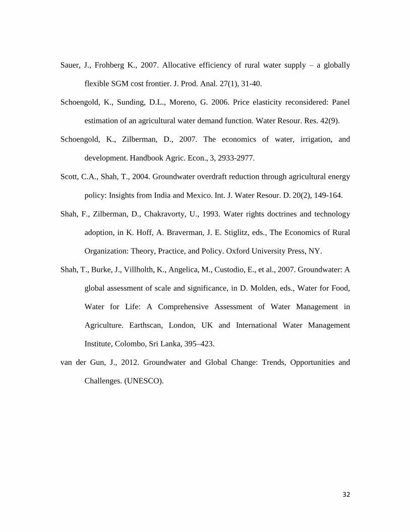
illustrated in Figure 1 by a clockwise rotation of the marginal cost curve from 𝑀𝐶𝑖𝑤 to

𝑀𝐶𝑖𝑤,𝑠

. Figure 1 also depicts a decreasing marginal revenue curve due to decreasing

marginal productivity of irrigation. The combination of a clockwise rotation of marginal

cost and a downward sloping marginal revenue curve causes an increase in pumping. The

overall effect of the electricity subsidy on pumping will be determined by the magnitude

of the subsidy and the marginal productivity of irrigation beyond 𝑄𝑖𝑤.

Sharing of Wells among Farmers

The description of marginal cost of pumping in the previous section assumed a well is

operated by a single farmer. However, different wells in Mexico function under different

institutional arrangements. Some wells are individually owned while others are shared by

multiple farmers. Table 1 describes the percentage of wells that are either owned by a single

producer or jointly shared by multiple producers. As expected, we observe a large number

of wells that are shared by multiple irrigators.

Models formalizing cost and strategic externalities (Provencher and Burt 1993)

show that sharing of water resources by multiple irrigators may decrease marginal cost and

aggravate over-extraction. Moreover these analyses have demonstrated that an increased

number of irrigators sharing the resource is associated with greater pumping. As revealed

by Table 1 the majority of wells (61 percent) are shared by multiple irrigators. Table 1 also

shows the distribution of the number of users per well in our sample. The mean number of

users is about 12. While the median size of the group is 6, about a quarter of wells are

10

shared by more than 16 farmers. These figures suggest that inefficiencies or over-extraction

due well sharing may be quantitatively relevant for Mexico’s aquifers.

When multiple farmers share a well, the depth of the water table is influenced by

the sum of individual pumping rates. Moreover each farmer’s pumping has the same effect

on the depth to the water table such that 𝐻 = 𝜇 + ∑ 휀𝑤𝑖𝑖 ; where 𝑤𝑖 represents the

𝑖𝑡ℎfarmer’s pumping rate, 휀 is the increase in depth per unit of water pumped, and the rest

is as before. Thus, the unit cost of water for farmer 𝑖 who shares a well with other farmers

is:

𝑃𝑖𝑤,𝑠+𝑤𝑠 = [𝑝𝑘𝑤ℎ − 𝑣𝑘𝑤ℎ](𝑎 + 𝑏(𝑤𝑖 + ∑ 𝑤𝑗𝑗≠𝑖 )) (5)

where 𝑃𝑖𝑤,𝑠+𝑤𝑠

denotes unit cost of water under an electricity subsidy and well-sharing,

with 𝑤𝑠 in the superscript indicating well sharing, and the rest is as defined before.

Based on (5), marginal cost can be expressed as:

𝑀𝐶𝑖𝑤,𝑠+𝑤𝑠 = [𝑝𝑘𝑤ℎ − 𝑣𝑘𝑤ℎ]((𝑎 + 𝑏𝑊) + 𝑏𝑤𝑖(1 + 𝜌)) (6)

where 𝑀𝐶𝑖𝑤,𝑠+𝑤𝑠

denotes marginal pumping cost of water under an electricity subsidy and

well-sharing; 𝑊 = ∑ 𝑤𝑖𝑁𝑖=1 = 𝑤𝑖 + ∑ 𝑤𝑗𝑗≠𝑖 ; 𝜌 is a parameter representing farmer 𝑖’s

conjecture about others’ reactions to her pumping decisions; 𝜌 = ∑𝜕𝑤𝑗

𝜕𝑤𝑖𝑗≠𝑖 . This parameter

typically captures the degree to which pumping rates by different farmers are strategic

substitutes 𝜌 < 0 or strategic complements 𝜌 > 0. The parameter 𝜌 is typically considered

to range between 1 and −1.

The effect of both distortions (electricity subsidy and well-sharing) combined is

captured in Figure 1 by a clockwise rotation of marginal cost of pumping from 𝑀𝐶𝑖𝑤 to

11

𝑀𝐶𝑖𝑤,𝑠+𝑤𝑠

. The specific distortionary effect of well-sharing is depicted as the wedge

between 𝑀𝐶𝑖𝑤,𝑠

and 𝑀𝐶𝑖𝑤,𝑠+𝑤𝑠

. The magnitude of the increase in pumping caused by well-

sharing depends on the size of this wedge and the slope of the marginal revenue curve.

The magnitude of the rotation in marginal cost caused by well-sharing depends on

the strength of the cost and strategic externalities previously discussed. A key parameter to

both externalities is the drawdown faced by one farmer when another extracts water. When

multiple farmers draw from the same well, drawdown caused by one farmer’s extraction

affects everyone sharing the well equally so the effect of the cost and strategic externalities

is potentially large. In other words, the magnitude of the clockwise rotation of the marginal

cost curve in Figure 1 may be considerable.

Electricity Cost sharing

With multiple producers, it can be difficult to calculate individual water use from a shared

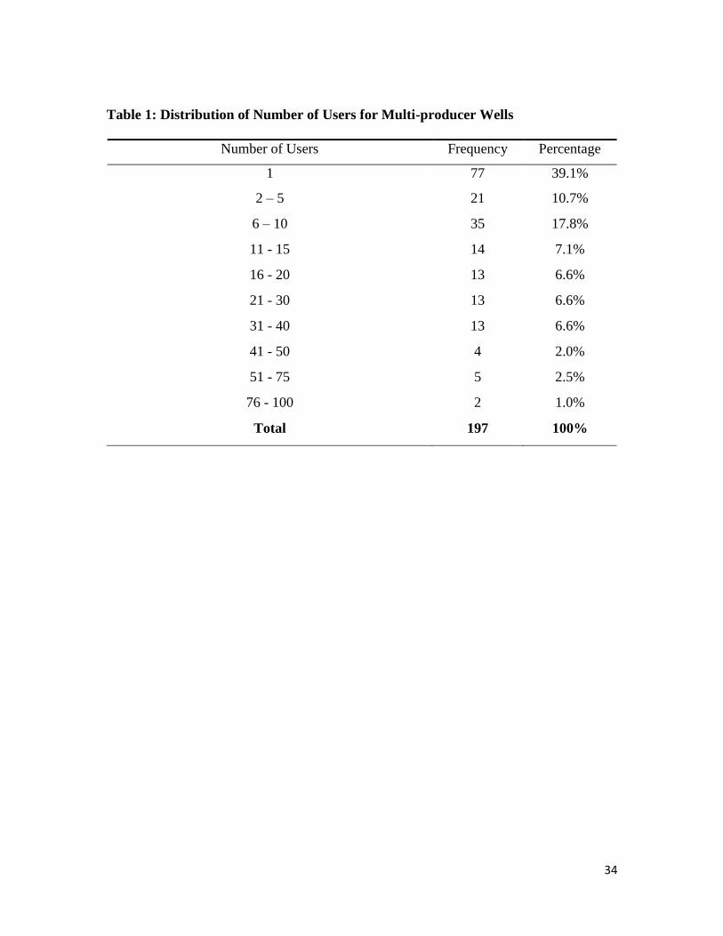
well without the appropriate metering technology. Table 2 shows how the electricity costs

for irrigation water are distributed between users. About 38 percent of the wells base the

cost on the number of hours an individual irrigates (this means that farmers do not share

the cost of electricity but rather pay for their own consumption), while 38 percent divide

the cost based on land area and another 25 percent split cost in equal shares. The remaining

77 wells are owned by a single producer. The distribution of cost-share rules across our

sample gives us enough variability to quantify the effect of these cost-share rules on

irrigation efficiency.

12

Distributing the cost of electricity based on pre-specified payment rules may

introduce further distortions in marginal cost of pumping. To model the distortions of cost-

share rules, we consider the case of a farmer that pays a pre-specified share 𝑠𝑖 of the total

electricity bill. The unit cost of water in this case is:

𝑃𝑖𝑤,𝑠+𝑤𝑠+𝑐𝑠 = [𝑝𝑘𝑤ℎ − 𝑣𝑘𝑤ℎ] (𝑎 + 𝑏(𝑤𝑖 + ∑ 𝑤𝑗𝑗≠𝑖 ))

𝑊𝑠𝑖

𝑤𝑖 (7)

where 𝑃𝑖𝑤,𝑠+𝑤𝑠+𝑐𝑠

denotes unit cost of water under cost share with 𝑐𝑠 in the superscript

indicating cost sharing, 𝑠𝑖 is the share of total electricity bill paid by the 𝑖𝑡ℎ farmer and the

rest is as before. If electricity cost is split based on land area, 𝑠𝑖 =𝐿𝑖

𝐿, where 𝐿𝑖 is the land

endowment of the 𝑖𝑡ℎ farmer and 𝐿 is total land area irrigated with water from the well. On

the other hand, if electricity cost is split evenly among farmers, 𝑠𝑖 =1

𝑁, where 𝑁 is the total

number of farmers drawing water from the same well.

The marginal cost of pumping can then be denoted by:

𝑀𝐶𝑖𝑤,𝑠+𝑤𝑠+𝑐𝑠 = [𝑝𝑘𝑤ℎ − 𝑣𝑘𝑤ℎ](1 + 𝜌)(𝑎 + 2𝑏𝑊)𝑠𝑖 (8)

where 𝑀𝐶𝑖𝑤,𝑠+𝑤𝑠+𝑐𝑠

denotes marginal cost of water under subsidy, well share, and cost

share and the rest was defined before.

We are interested in identifying conditions under which electricity cost sharing may

reduce the marginal cost of pumping and exacerbate over-extraction. Such a situation

occurs whenever 𝑀𝐶𝑖𝑤,𝑠+𝑤𝑠+𝑐𝑠 < 𝑀𝐶𝑖

𝑤,𝑠+𝑤𝑠, which is found to be satisfied if (1 + 𝜌)𝑠𝑖 <

1 (derivation of this condition and further discussion can be found in Appendix A). Given

the share of the electricity bill assigned to a given farmer, one farmer’s pumping increases

other farmers’ cost even in the absence of drawdown (i.e. even in the absence of cost and

13

strategic externality). This is due to an increase in others’ unit cost of water as revealed by

equation (7). Equation (7) shows that sharing the cost of electricity creates another source

of non-excludability resulting from the fact that individual farmers cannot exclude others

from their own electricity expenditure. We call this externality the “cost-share externality”.

The effect of the cost-share externality with subsidized electricity rates is illustrated

in Figure 1 by a clockwise rotation of the marginal cost of pumping from 𝑀𝐶𝑖𝑤 to

𝑀𝐶𝑖𝑤,𝑠+𝑤𝑠+𝑐𝑠

. The specific distortionary effect of cost sharing is depicted as the wedge

between 𝑀𝐶𝑖𝑤,𝑠+𝑤𝑠

and 𝑀𝐶𝑖𝑤,𝑠+𝑤𝑠+𝑐𝑠

. The magnitude of the increase in water pumped

caused by cost sharing will depend upon the size of this wedge and the slope of the marginal

revenue curve. In turn, the size of the wedge depends upon the farmer’s share of electricity

bill and their conjectures about others’ reactions to their pumping decisions (parameters 𝑠𝑖

and ).

Formalization and graphical illustration of the effect of multiple distortions

prevalent in Mexico on marginal cost of pumping allows us to generate testable hypotheses.

We now proceed to discuss our hypotheses regarding the drivers of inefficient over-

extraction and our strategy for empirical assessment of those hypotheses.

Hypotheses of this Study

From our discussion of distortions to the marginal cost of pumping, it follows that the

number of farmers sharing a well and electricity cost sharing are both expected to increase

groundwater use. But in line with findings in previous studies in other countries and

14

institutional contexts (e.g. Hendricks and Peterson 2012), we expect water demand to be

inelastic to its unitary price.

Testing the hypothesis of inelastic water demand requires estimating irrigation

demand and its own price elasticity. Due to potential inefficiencies associated with

institutional distortions, the dual frontier (e.g. cost or profit functions) is not a neutral

transformation of the frontier augmented to incorporate inefficiency and estimates of water

demand elasticity from the former may be biased (Kumbhakar 2001). Therefore we

estimate a frontier irrigation demand function and allow for inefficiency in the application

of irrigation water. We exploit the estimated frontier to measure the effect of the number

of farmers sharing a well and the electricity cost-share rules on irrigation efficiency.

Radial measures of inefficiency (either input-based or output-based) preclude

decomposition of inefficiency scores with respect to a single production input masking

differences in efficiency that might be attributed to particular factor inputs (Kopp 1981).

This is a limitation worth avoiding, especially when there are reasons to suspect that certain

production factors may be used particularly inefficiently. This may be the case with

irrigation given the institutional arrangements distorting its marginal cost. Failure to

identify inefficiency attributable to a specific input factor hinders input-specific policy

design (Sauer and Frohberg 2007). To gauge efficiency in irrigation application, we use an

input-specific measure of efficiency developed by Kumbhakar (1989).

Model

15

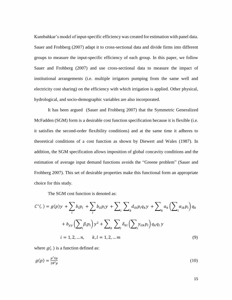
Kumbahkar’s model of input-specific efficiency was created for estimation with panel data.

Sauer and Frohberg (2007) adapt it to cross-sectional data and divide firms into different

groups to measure the input-specific efficiency of each group. In this paper, we follow

Sauer and Frohberg (2007) and use cross-sectional data to measure the impact of

institutional arrangements (i.e. multiple irrigators pumping from the same well and

electricity cost sharing) on the efficiency with which irrigation is applied. Other physical,

hydrological, and socio-demographic variables are also incorporated.

It has been argued (Sauer and Frohberg 2007) that the Symmetric Generalized

McFadden (SGM) form is a desirable cost function specification because it is flexible (i.e.

it satisfies the second-order flexibility conditions) and at the same time it adheres to

theoretical conditions of a cost function as shown by Diewert and Wales (1987). In

addition, the SGM specification allows imposition of global concavity conditions and the

estimation of average input demand functions avoids the “Greene problem” (Sauer and

Frohberg 2007). This set of desirable properties make this functional form an appropriate

choice for this study.

The SGM cost function is denoted as:

𝐶∗(. ) = 𝑔(𝑝)𝑦 + ∑ 𝑏𝑖𝑝𝑖 + ∑ 𝑏𝑖𝑖𝑝𝑖𝑦

𝑖𝑖

+ ∑ 𝑖

∑ 𝑑𝑖𝑘𝑝𝑖𝑞𝑘𝑦𝑘

+ ∑ 𝑎𝑘 (∑ 𝛼𝑖𝑘𝑝𝑖𝑖

) 𝑞𝑘𝑘

+ 𝑏𝑦𝑦 (∑ 𝛽𝑖𝑝𝑖𝑖

) 𝑦2 + ∑ 𝑘

∑ 𝛿𝑘𝑙 (∑ 𝛾𝑖𝑙𝑘𝑝𝑖𝑖

) 𝑞𝑘𝑞𝑙𝑙

𝑦

𝑖 = 1, 2, … 𝑛, 𝑘, 𝑙 = 1, 2, … 𝑚 (9)

where 𝑔(. ) is a function defined as:

𝑔(𝑝) =𝑝′𝑆𝑝

2𝜃′𝑝 (10)

16

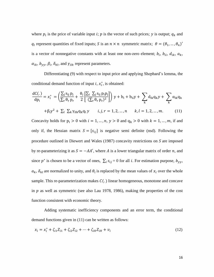
where 𝑝𝑖 is the price of variable input 𝑖; 𝑝 is the vector of such prices; 𝑦 is output; 𝑞𝑘 and

𝑞𝑙 represent quantities of fixed inputs; 𝑆 is an 𝑛 × 𝑛 symmetric matrix; 𝜃 = (𝜃1, … , 𝜃𝑛)′

is a vector of nonnegative constants with at least one non-zero element; 𝑏𝑖, 𝑏𝑖𝑖, 𝑑𝑖𝑘, 𝑎𝑘,

𝛼𝑖𝑘, 𝑏𝑦𝑦, 𝛽𝑖, 𝛿𝑘𝑙, and 𝛾𝑖𝑙𝑘 represent parameters.

Differentiating (9) with respect to input price and applying Shephard’s lemma, the

conditional demand function of input 𝑖, 𝑥𝑖∗, is obtained:

dC(. )

dpi= 𝑥𝑖

∗ = (∑ sijj pj

∑ θrr pr+

θ𝑖

2[∑ i ∑ sijj pipj

(∑ θrr pr)2]) y + bi + biiy + ∑ dikqk𝑦

k

+ ∑ αikqk

k

+βiy2 + ∑ l ∑ γilkqkqlk 𝑦 𝑖, 𝑗, 𝑟 = 1, 2, … , 𝑛 𝑘, 𝑙 = 1, 2, … , 𝑚. (11)

Concavity holds for pi > 0 with 𝑖 = 1, … , 𝑛, 𝑦 > 0 and qk > 0 with 𝑘 = 1, … , 𝑚, if and

only if, the Hessian matrix 𝑆 = [𝑠𝑖𝑗] is negative semi definite (nsd). Following the

procedure outlined in Diewert and Wales (1987) concavity restrictions on 𝑆 are imposed

by re-parameterizing it as 𝑆 = −𝐴𝐴′, where 𝐴 is a lower triangular matrix of order 𝑛, and

since 𝑝∗ is chosen to be a vector of ones, ∑ 𝑠𝑖𝑗 𝑖 = 0 for all 𝑖. For estimation purpose, 𝑏𝑦𝑦,

𝑎𝑘, 𝛿𝑘𝑙 are normalized to unity, and 𝜃𝑖 is replaced by the mean values of 𝑥𝑖 over the whole

sample. This re-parameterization makes 𝐶(. ) linear homogeneous, monotone and concave

in 𝑝 as well as symmetric (see also Lau 1978, 1986), making the properties of the cost

function consistent with economic theory.

Adding systematic inefficiency components and an error term, the conditional

demand functions given in (11) can be written as follows:

𝑥𝑖 = 𝑥𝑖∗ + 휁𝑖1𝑍𝑖1 + 휁𝑖2𝑍𝑖2 + ⋯ + 휁𝑖𝐻𝑍𝑖𝐻 + 𝑣𝑖 (12)

17

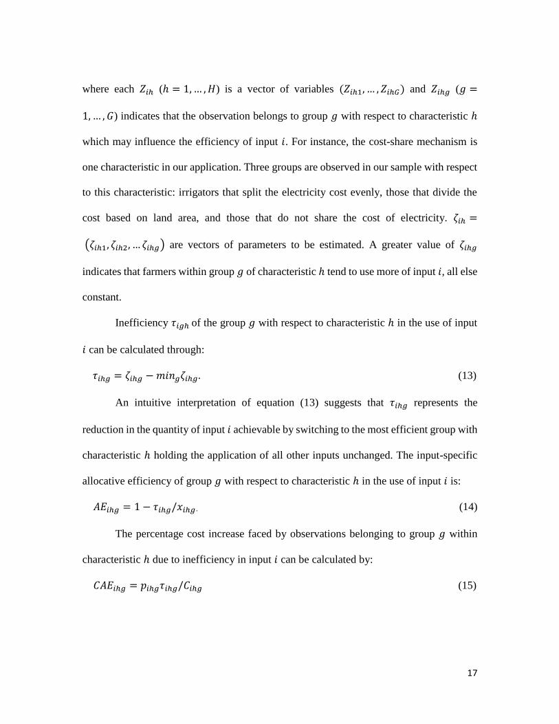
where each 𝑍𝑖ℎ (ℎ = 1, … , 𝐻) is a vector of variables (𝑍𝑖ℎ1, … , 𝑍𝑖ℎ𝐺) and 𝑍𝑖ℎ𝑔 (𝑔 =

1, … , 𝐺) indicates that the observation belongs to group 𝑔 with respect to characteristic ℎ

which may influence the efficiency of input 𝑖. For instance, the cost-share mechanism is

one characteristic in our application. Three groups are observed in our sample with respect

to this characteristic: irrigators that split the electricity cost evenly, those that divide the

cost based on land area, and those that do not share the cost of electricity. 휁𝑖ℎ =

(휁𝑖ℎ1, 휁𝑖ℎ2, … 휁𝑖ℎ𝑔) are vectors of parameters to be estimated. A greater value of 휁𝑖ℎ𝑔

indicates that farmers within group 𝑔 of characteristic ℎ tend to use more of input 𝑖, all else

constant.

Inefficiency 𝜏𝑖𝑔ℎ of the group 𝑔 with respect to characteristic ℎ in the use of input

𝑖 can be calculated through:

𝜏𝑖ℎ𝑔 = 휁𝑖ℎ𝑔 − 𝑚𝑖𝑛𝑔휁𝑖ℎ𝑔. (13)

An intuitive interpretation of equation (13) suggests that 𝜏𝑖ℎ𝑔 represents the

reduction in the quantity of input 𝑖 achievable by switching to the most efficient group with

characteristic ℎ holding the application of all other inputs unchanged. The input-specific

allocative efficiency of group 𝑔 with respect to characteristic ℎ in the use of input 𝑖 is:

𝐴𝐸𝑖ℎ𝑔 = 1 − 𝜏𝑖ℎ𝑔/𝑥𝑖ℎ𝑔 . (14)

The percentage cost increase faced by observations belonging to group 𝑔 within

characteristic ℎ due to inefficiency in input 𝑖 can be calculated by:

𝐶𝐴𝐸𝑖ℎ𝑔 = 𝑝𝑖ℎ𝑔𝜏𝑖ℎ𝑔/𝐶𝑖ℎ𝑔 (15)

18

where 𝐶𝑖ℎ𝑔 is observed total production cost of farmers in group 𝑔 with respect to

characteristic ℎ.

The measure 𝐶𝐴𝐸𝑖ℎ𝑔 allows identification of the inputs with the greatest potential

for cost savings because it weighs input quantity reductions by their respective prices. As

explained by Kumbhakar (1989), one of the advantages of this procedure is that no special

distributional assumptions are needed on 𝜏𝑖ℎ𝑔, as independence between 𝜏𝑖ℎ𝑔 and other

regressors in the demand system is not required.

Data

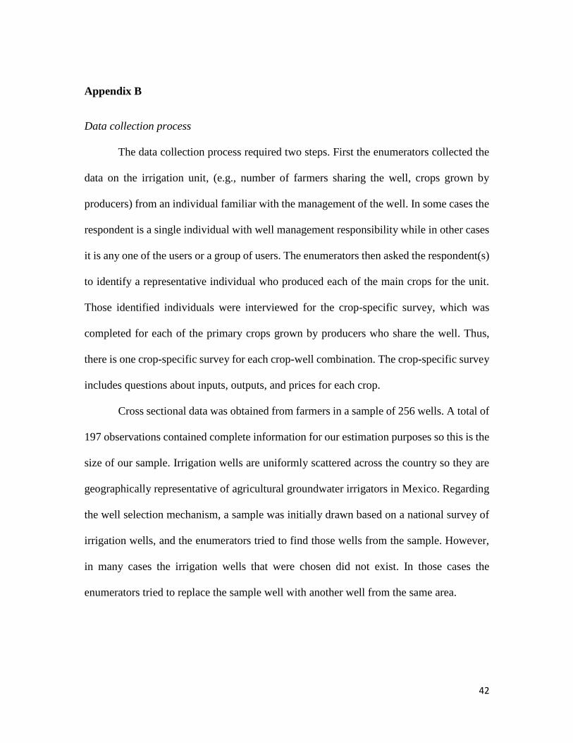
A survey of agricultural groundwater irrigators was conducted in Mexico by the Instituto

Nacional de Ecología y Cambio Climático (National Institute of Ecology and Climate

Change). Data collection on irrigation wells occurred during the 2003-2004 winter. A

detailed description of the data collection process can be found in Appendix B.

Cross sectional data was obtained from farmers in a sample of 197 wells. Irrigation

wells are uniformly scattered across the country so they are geographically representative

of agricultural groundwater irrigators in Mexico. Detailed data on quantities and prices of

inputs and outputs were obtained from farmers along with data on irrigation application

and cost of electricity used in pumping groundwater. The data includes quantities and

prices of three variable inputs (fertilizer, irrigation, and a composite of other inputs

including expenditures in land rent and preparation, labor, pesticide, and marketing), and

one fixed input (land). A vector of outputs including field crops, fruits, and vegetables were

19

aggregated into one single output applying Jorgenson’s procedure for “exact” aggregation

(Jorgenson, Gollop and Fraumeni 1987).

Potential sources of inefficiency (i.e. elements of vector 𝑍𝑖ℎ in equation (12))

considered in this study are: mechanism for sharing electricity costs (no cost sharing,

evenly split, or based on area), and the number of farmers in each well (i.e. which can

presumably capture pressures from strategic pumping). Control variables include socio-

demographic, biophysical, and hydrological variables. Variability in irrigation technology

is not observed as the overwhelming majority of farmers (96 percent in our sample) use

gravity irrigation systems.

Table 2 reports the mean and standard deviation of variables by type of cost share.

Some variables have similar distributions in all four groups. For example, the farmer’s age

and soil type are similar for all four groups. However, we do find some systematic

differences across groups. Irrigation units that have no cost share (individually-owned

wells and the wells that everyone pays for his/her own water use) have a substantially

higher average land area (mean of 34.9 and 30.7 hectares) than farmers operating under

equal share (7.2 hectares) and share based on land area (8.5 hectares). The education level

of farmers with no cost share is higher compared to those with a cost share. These

correlations underscore the importance of controlling for education and land area when

quantifying the marginal effect of cost share on irrigation efficiency.

Estimation

20

Following Provencher and Burt (1993), the number of farmers sharing a well is included

as an explanatory variable in our estimation. Binary indicators for each electricity cost-

sharing mechanism (evenly-based and area-based) are also included. The effect of these

variables on irrigation may be confounded with the effect of other drivers such as soil type,

climate regime, depth to groundwater, age and education of farmers, and crop types.

Obtaining reliable estimates of the link between well sharing, cost-share rules and pumping

requires controlling for these factors.

The system of equations is specified as:

𝑥𝑖 = 𝑥𝑖∗ + 𝑎𝑛𝑖 ∗ 𝑁 + 𝑎𝑐𝑠1𝑖 ∗ 𝐶𝑆1 + 𝑎𝑐𝑠2𝑖 ∗ 𝐶𝑆2 + 𝑎𝑠𝑖𝑖 ∗ 𝑆𝐼 + 𝑎𝑐𝑙𝑖 ∗ 𝐶𝐿

+𝑎𝑑𝑒𝑝𝑡ℎ𝑖 ∗ 𝐷𝐸𝑃𝑇𝐻 + 𝑎𝑎𝑔𝑒𝑖 ∗ 𝐴𝐺𝐸 + 𝑎𝑒𝑑𝑢𝑖 ∗ 𝐸𝐷𝑈𝐶𝐴𝑇𝐼𝑂𝑁 + 𝑎𝑦𝑓𝑣𝑖 ∗ 𝑌𝐹𝑉 + 𝑣𝑖

𝑖 = 𝑤𝑎𝑡𝑒𝑟, 𝑓𝑒𝑟𝑡𝑖𝑙𝑖𝑧𝑒𝑟, 𝑜𝑡ℎ𝑒𝑟 𝑖𝑛𝑝𝑢𝑡𝑠 (16)

where 𝑥𝑖∗ is defined by equation (11) which captures the impact of prices of inputs, outputs,

and fixed inputs, 𝑁 is the number of farmers sharing a well, and 𝐶𝑆1 and 𝐶𝑆2 are the cost-

share dummies.

Equation system (16) also includes controls for soil type (𝑆𝐼 = 1, … ,5, where 𝑆𝐼 =

1 for finest soil and 𝑆𝐼 = 5 for coarsest), depth of well (𝐷𝐸𝑃𝑇𝐻) measured in meters to

water table, age of the farmer (AGE), education of the farmer (EDUCATION) (i.e. (1) did

not finish elementary school, (2) finished elementary school, (3) finished middle-school,

(4) finished high-school, (5) more than high-school),2 climate zone (CL), and crop types

2 Education may be more appropriately captured by a dummy variable for each level of schooling.

However, this would create 4 more variables in each equation which would result in a significant increase

in the number of parameters to be estimated. Measuring education by a categorical variable increases the

parsimony of our model and eases the burden on degrees of freedom with only 197 observations.

21

(YFV) which is captured by the share of fruit and vegetable in total output as these crops

tend to be more water intensive than field crops.

The climate zones are based on the widely used Köppen-Geiger classification

system, which are used internationally for consistency between nations and regions.

Mellinger, Sachs and Gallup (1999) provide an excellent description of the classification

system. Since the climate zones are not ordered based on expected precipitation or

irrigation requirements, we create two categorical variables for the empirical analysis.3 The

default (omitted) category refers to regions with a temperate climate and a dry winter, while

the alternative category refers to regions with a semi-arid or arid climate. We expect that

irrigation requirements will be lower in the default category than the alternative category.

With shared wells we do not have sufficient information to attribute input usage

and output production to specific farmers so we use the average age and education of

surveyed farmers as the socio-demographic variables for the unit. Output includes field

crops, fruits, and vegetables. Fruits and vegetables are typically more water intensive than

field crops so we include the combined share of fruits and vegetables in total output.

The system (16) is estimated using a nonlinear iterative seemingly unrelated

regression estimator with Eicker-Huber-White heteroskedastic-consistent standard errors.4

With three inputs, the matrix 𝑆𝑖𝑗 is a 3 by 3 matrix, which is recovered from estimation of

matrix A.

3 The limited number of degrees of freedom makes it impossible to estimate coefficients for seven

categorical variables based on each unique climate zone. 4 To impose concavity on the cost function, we have to estimate Aij instead of Sij. While Sij are linear in our

model, Aij are not. As a result, a nonlinear SUR regression is used instead of linear regression.

22

Results

Demand equations for water, fertilizer and the composite of other inputs are estimated

simultaneously and their R-square values are 0.74, 0.59, and 0.86 respectively. The

coefficients for correlation of error terms across equations are -0.13, 0.10 and -0.02 for

water and fertilizer equations, water and the composite input, and fertilizer and the

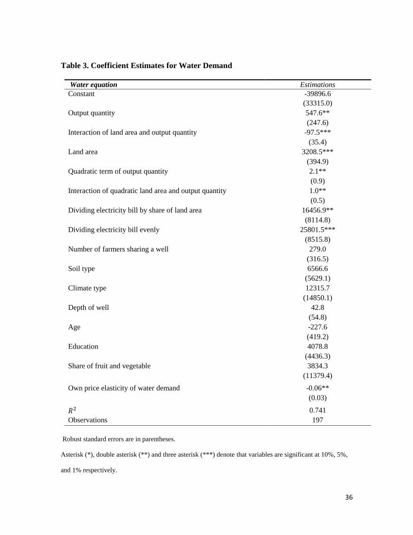
composite input equations respectively.5 Table 3 reports estimation results of the water

equation. Results for the other two inputs are reported in Table C.1 in Appendix C. The

number of farmers sharing a well does not have a statistically significant impact on

irrigation application. This result suggests that strategic pumping caused by well-sharing

is weak, at best.6

Sharing the cost of electricity evenly has a positive and statistically significant

impact on irrigation application. Sharing the cost of electricity based on land area also has

a positive but smaller impact. Results of cost-share variables are consistent with the

hypothesis that cost sharing reduces irrigation-use efficiency.

To ensure that the effect of cost sharing is not being confounded with the effect of

well-sharing, we have also estimated the model with the sub-sample of shared wells only.

The effect of electricity cost sharing is robust to this change, though the reduction in sample

size reduces the precision of the coefficients.

5 The null hypothesis of no correlation across error terms in the system is strongly rejected at the 1% level

of significance with a likelihood ratio of 3690.5 (critical value of 11.34). 6 The model was also estimated with a quadratic term for 𝑁 and interaction terms between 𝐶𝑆1, 𝐶𝑆2 and 𝑁

to consider different channels through which well sharing might affect irrigation. We have also estimated a

model where 𝑁 was replaced by a well share dummy. Well sharing had an insignificant effect across all

models.

23

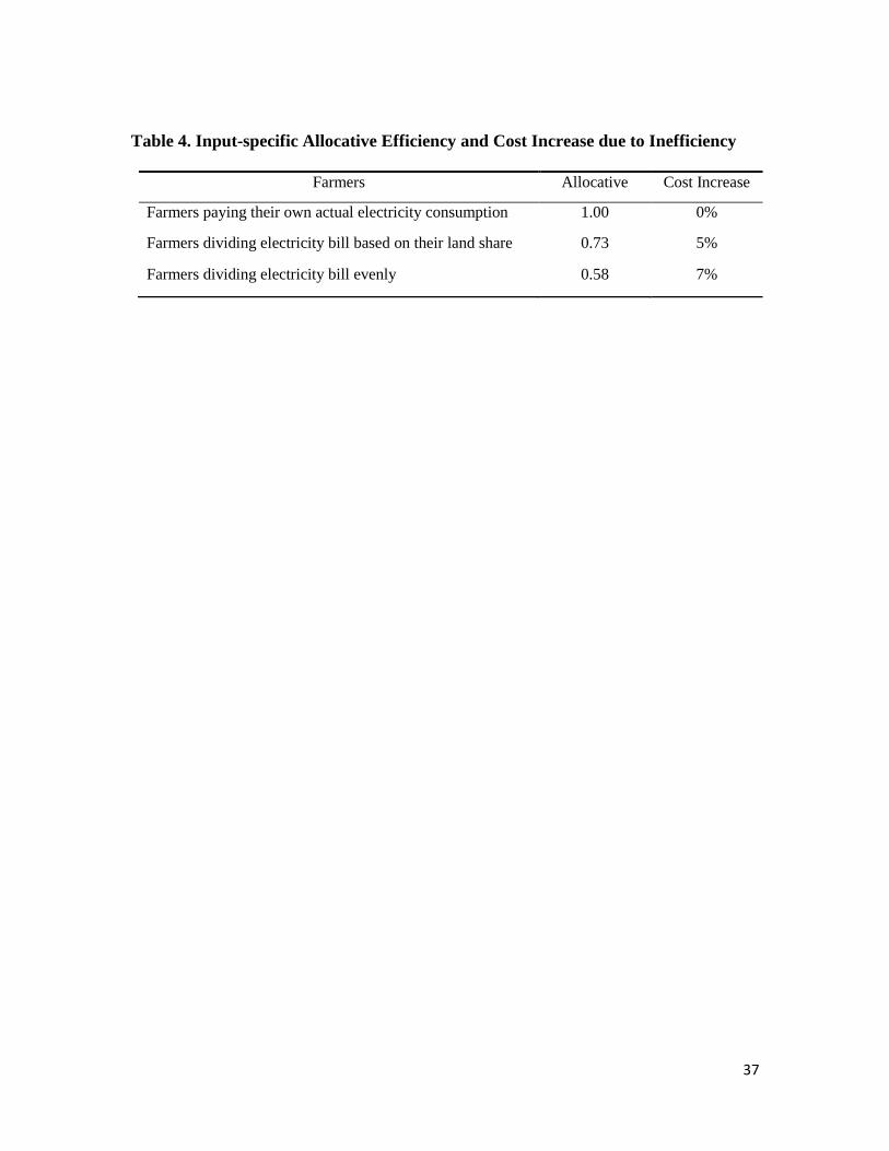
Parameter estimates are used to calculate efficiency as described by equations (13)

and (14) and results are reported in Table 4. Implementing an evenly split cost-share

mechanism decreases farmers’ irrigation efficiency to 0.58 while implementing a land-

based cost-share mechanism decreases farmers’ irrigation efficiency to 0.73. These results

show that a cost-share rule which splits the electricity cost evenly among farmers has a

stronger effect than a rule establishing cost share based on land area.

Our results show that the cost distortion introduced by electricity cost sharing is

substantial. Cost sharing creates a situation where a farmer pays only a fraction of the

electricity cost of his/her extra pumping. Under an evenly split cost-share rule this is

perhaps a small fraction of total electricity cost (e.g. only 20% in a well shared by 5

farmers). Under a land-share rule, larger farmers may not benefit as much as their smaller

counterparts. Consequently the effect of an evenly-split cost-share rule is found to be larger

in magnitude and statistically more robust, than a cost-share rule based on land area.

Our results suggest that distortions caused by the cost and strategic externalities

(i.e. the magnitude of the clockwise rotation from 𝑀𝐶𝑖𝑤,𝑠 to 𝑀𝐶𝑖

𝑤,𝑠+𝑤𝑠 in Figure 1) are not

strong. This may be explained by a small impact of individual pumping on the water level,

absence of strategic pumping from farmers sharing the well, or by unobservable self-

governance institutions facilitating cooperative behavior. However, if such institutions

were effective enough to eliminate the marginal cost-reducing effects of well-sharing, they

would also eliminate the effect of electricity cost-sharing mechanisms (rotation from

𝑀𝐶𝑖𝑤,𝑠+𝑤𝑠 to 𝑀𝐶𝑖

𝑤,𝑠+𝑤𝑠+𝑐𝑠 in Figure 1), which does not seem to be the case. Therefore, while

the influence of hydrological and institutional features cannot be distinguished in our

24

analysis, results suggest that the insignificant effect of well sharing on pumping is

explained by a small impact of an individual's pumping on water level or absence of

strategic pumping, rather than the existence of cooperative institutions.

Allocative inefficiency in irrigation application results in production cost that is

higher than the minimum cost. The increase in cost for farmers operating under each cost-

share mechanism can be calculated based on equation (15). The percentage increase in cost

due to allocative inefficiency with cost sharing is reported in Table 4. We find that

allocative inefficiency associated with area-based (evenly-based) cost share increases total

production cost by 5 (7) percent. Therefore in addition to having a significant impact on

the overall amount of water pumped, irrigation inefficiency also has a sizable effect on

overall production costs. This suggests that removal of inefficiency sources will not only

alleviate groundwater depletion but also improve farmers’ welfare.

The own price elasticity of demand for irrigation water is reported in Table 3 and

it is -0.06 (with a bootstrapped standard deviation of 0.02 so the elasticity estimate is

significant at 5% level), which means that a doubling of the unitary cost of pumping would

reduce irrigation by 6 percent. Thus, only a very substantial increase in pumping cost can

have a sizable impact on irrigation.

Some limitations of this analysis are worth noting. The cross sectional nature of our

data does not allow us to control for unobservable fixed effects that may be correlated with

our explanatory variables. We are able to control for some important time-invariant factors

such as soil, climate, and socio-demographic variables, but analysis with cross-sectional

25

data always risks omitted variable bias due to correlation between unobservables and

explanatory variables.

This analysis, like the rest of the literature, neglects issues of optimal timing of

irrigation. Inefficiencies can emerge not only in terms of the total amount of water applied

during the growing season but also in terms of the timing of application. Farmers that share

the same well may play a dynamic game in which they deviate from the optimal irrigation

schedule if they believe they avoid the drawdown caused by another farmer at the otherwise

optimal irrigation time. Finally, a profit maximizing framework may be more appropriate

for farmers in this context. However, theoretically consistent and econometrically

implementable input specific efficiency measures in the context of a profit dual function

are not yet available. Expanding input-specific-efficiency measures in this direction seems

to be a relevant and promising research avenue.

Policy Implications

In combination our results show that common pool problems created by the sharing of

electricity cost can have a sizable impact on pumping. As summarized by Ostrom in several

studies (e.g. Ostrom 1996), conventional solutions to the common pool problem typically

include creation of property rights (granting the property of the well to one individual or

institution) and government ownership and control. The former can have significant

implementation problems and resistance in the field. For the latter to effectively reduce

over-extraction regulators would have to: 1) pursue maximization of social welfare as their

26

objective; 2) have knowledge of the workings of ecological and hydrological systems; and

3) have knowledge of institutional changes that would induce socially optimal behavior.

An alternative solution that is frequently observed in the field and was formalized

by Ostrom et al. (1999) is that of self-governance. Our results seem to indicate that self-

governance institutions inducing cooperative behavior may not have been in place in

Mexico during the time of the survey or that they were not sufficient to prevent

considerable inefficiency from the common pool problem created by electricity cost-

sharing rules. Self-governance cannot be successfully implemented everywhere.

Conditions like feasible improvement of the resource, trust among users, and users’

discount rate influence the chances of successful self-governance of a natural resource.

Therefore the success of these institutional reforms will be determined by the

idiosyncrasies of wells and regions in Mexico. An ex-ante evaluation of alternative

institutional arrangements to solve the common pool problem of groundwater in Mexico

constitutes an undoubtedly important research avenue in the future.

A much simpler, yet promising solution to the cost-share problem is facilitating

implementation of metering systems and allocation rules that allow charging each farmer

for his own consumption. This is especially true for those wells that divide electricity costs

evenly among farmers. In some cases, there may be financial barriers to adoption of these

technologies and, in others, social ones. Public policies should be aimed at removing the

barriers preventing adoption of more modern metering systems.

The magnitude of the own price elasticity of demand suggests that elimination of

the electricity subsidy by itself is not an effective policy for a significant reduction of

27

groundwater pumping. This result, along with the impact of cost-share variables on

irrigation demand, suggest that elimination of cost-share mechanisms seems a much more

promising conservation policy than price-based instruments. In addition, intuition suggests

that the latter will have a negative effect on farmers’ welfare while the former, by

eliminating cost inefficiencies shown in Table 4, may result in higher welfare for farmers.

Conclusions

The objective of this study was to quantify the role of different sources of non-excludability

on irrigation water demand in Mexico. We model three potential distortions of the marginal

pumping cost of groundwater, and empirically gauge their impacts on irrigation demand.

Based on insights from a theoretical model of the marginal cost of pumping, we

hypothesize that electricity subsidies, well sharing, and electricity cost sharing will increase

groundwater pumping and aggravate groundwater depletion.

Our results are consistent with the hypothesis that electricity cost sharing decreases

farmers’ irrigation efficiency. In fact, results suggest that cost sharing is at the heart of

water over-extraction observed in many areas in Mexico. Both cost-share rules have a

statistically and quantitatively significant effect on pumping. Moreover, our results are

consistent with the hypothesis that water demand is inelastic and, thus, eliminating the

electricity subsidy is unlikely to result in a substantial reduction in irrigation. We estimate

that the price elasticity of irrigation is only -0.06, which means that a doubling of the

unitary cost of pumping would only reduce irrigation by 6 percent. In contrast, the

hypothesis that well sharing will decrease irrigation efficiency is rejected. Our results

28

indicate that the number of farmers sharing a well does not have a statistically significant

effect on individual pumping, which suggests either a limited effect of individual pumping

on water level or absence of strategic pumping by farmers sharing the wells.

Concerning the effect of these policies on farmers’ welfare, one needs to consider

that policy instruments reducing inefficiency need not cause a reduction in farmers’

surplus. This is because increases in individual marginal cost due to institutional reforms

may be offset by 1) reductions in pumping cost associated with a decrease in the total

volume pumped, and 2) an increase in water’s marginal value product due to enhanced

production efficiency. In other words the alleviation of externalities increases overall

welfare and this tends to offset the raise in individual pumping costs introduced by policy.

We suggest that policy makers consider all of these effects when making decisions about

changes to existing electricity and water policies.

29

References

Dhehibi, B., Lachaal, L., Elloumi, M., Messaoud, E.B., 2007. Measuring irrigation water

use efficiency using stochastic production frontier: An application on citrus

producing farms in Tunisia. Afr. J. Agric. Resour. Econ. 1(2), 1-15.

Diewert, W.E., Wales, T.J., 1987. Flexible functional form and global curvature conditions.

Econometrica, 55, 43–68.

Gisser, M., Sanchez, D.A., 1980. Competition versus optimal control in groundwater

pumping. Water Resour. Res. 16(4), 638-642.

Guevara-Sanginés, A., 2006. Water subsidies and aquifer depletion in Mexico’s arid

regions (No. HDOCPA-2006-23). Human Development Report Office (HDRO),

United Nations Development Programme (UNDP).

Hendricks, N.P., Peterson, J.M., 2012. Fixed effects estimation of the intensive and

extensive margins of irrigation water demand. J. Agr. Resour. Econ. 37(1), 1–19.

Howe, C.W., 2002. Policy issues and institutional impediments in the management of

groundwater: Lessons from case studies. Environ. Dev. Econ. 7(4), 625–641.

Huang, Q., Rozelle, S., Howitt, R., Wang J., Huang, J., 2010. Irrigation water demand and

implications for water pricing policy in rural China. Environ. Dev. Econ. 15(3),

293-319.

Huang, Q., Wang, J., Rozelle, S., Polasky, S., Liu, Y., 2013. The effects of well

management and the nature of the aquifer on groundwater resources. Am. J. Agric.

Econ. 95(1), 94-116.

30

Jorgenson, D.W., Gollop, F.M., Fraumeni, B.M., 1987. Productivity and U.S. Economic

Growth. Harvard University Press, Cambridge, MA.

Karagiannis, G., Tzouvelekas, V., Xepapadeas, A., 2003. Measuring irrigation water

efficiency with a stochastic production frontier: An application to Greek out-of-

season vegetable cultivation. Environ. Resour. Econ. 26, 57–72.

Kumbhakar, S.C., 1989. Estimation of technical efficiency using flexible functional form

and panel data. J. Bus. Econ. Stat. 7(2), 253-258.

Kumbhakar, S.C., 2001. Estimation of profit functions when profit is not maximum. Am.

J. Agric. Econ. 83(1), 1-19.

Kopp, R.J., 1981. The measurement of productive efficiency: A reconsideration. Q. J.

Econ. 96(3), 477–503.

Lau, L.J., 1978. Testing and imposing monotonicity, convexity and quasi-convexity

constraints, in M. Fuss and D. McFadden, eds., Production Economics: a Dual

Approach to Theory and Application, Vol. 1. Amsterdam: North-Holland, 409-453.

Lau L.J., 1986. Functional forms in econometric model building, in Z. Griliches, M. D.

Intriligator, eds., Handbook of Econometrics, Vol. 3, 1515–1565. North-Holland,

Amsterdam.

McGuckin, J.T., Gollehon, N., Ghosh, S., 1992. Water conservation in irrigated

agriculture: A stochastic production frontier model. Water Resour. Res. 28(2), 305-

312.

31

Mellinger, A.D., Sachs, J.D., Gallup, J.L., 1999. Climate, water navigability, and economic

development. Working Paper No. 24, Center for International Development,

Harvard University.

Negri, D.H., 1989. The common property aquifer as a differential game. Water Resour.

Res. 25(1), 9-15.

Ogg, C.W., Gollehon, N.R., 1989. Western irrigation response to pumping costs: A water

demand analysis using climatic regions. Water Resour. Res. 25(5), 767-773.

Ostrom, E., 1996. Crossing the great divide: Coproduction, synergy, and development.

World Dev. 24, 1073-1087.

Ostrom, E., Burger, J., Field, C.B., Norgaard, R.B., Policansky, D., 1999. Revisiting the

commons: Local lessons, global challenges. Science 284(5412), 278-282.

Pfeiffer. L., Lin, C-Y.C., 2012. Groundwater pumping and spatial externalities in

agriculture. J. Environ. Econ. Manag. 64(1), 16-30.

Provencher, B., Burt, O., 1993. The externalities associated with the common property

exploitation of groundwater. J Environ. Econ. Manag. 24(2), 139-158.

Provencher, B., Burt, O., 1994. A private property rights regime for the commons: The

case for groundwater. Am. J. Agric. Econ. 76(4), 875-888.

Rubio, S.J., Casino, B., 2001. Competitive versus efficient extraction of a common

property resource: The groundwater case. J. Econ. Dyn. Control 25(8), 1117-1137.

Rubio, S.J., Casino, B., 2003. Strategic behavior and efficiency in the common property

extraction of groundwater. Environ. Resour. Econ. 26(1), 73-87.

32

Sauer, J., Frohberg K., 2007. Allocative efficiency of rural water supply – a globally

flexible SGM cost frontier. J. Prod. Anal. 27(1), 31-40.

Schoengold, K., Sunding, D.L., Moreno, G. 2006. Price elasticity reconsidered: Panel

estimation of an agricultural water demand function. Water Resour. Res. 42(9).

Schoengold, K., Zilberman, D., 2007. The economics of water, irrigation, and

development. Handbook Agric. Econ., 3, 2933-2977.

Scott, C.A., Shah, T., 2004. Groundwater overdraft reduction through agricultural energy

policy: Insights from India and Mexico. Int. J. Water Resour. D. 20(2), 149-164.

Shah, F., Zilberman, D., Chakravorty, U., 1993. Water rights doctrines and technology

adoption, in K. Hoff, A. Braverman, J. E. Stiglitz, eds., The Economics of Rural

Organization: Theory, Practice, and Policy. Oxford University Press, NY.

Shah, T., Burke, J., Villholth, K., Angelica, M., Custodio, E., et al., 2007. Groundwater: A

global assessment of scale and significance, in D. Molden, eds., Water for Food,

Water for Life: A Comprehensive Assessment of Water Management in

Agriculture. Earthscan, London, UK and International Water Management

Institute, Colombo, Sri Lanka, 395–423.

van der Gun, J., 2012. Groundwater and Global Change: Trends, Opportunities and

Challenges. (UNESCO).

33

Figure 1. Sources of Distortions in Marginal Cost of Pumping

𝑀𝑅𝑖𝑤

𝑀𝐶𝑖𝑤,𝑠+𝑤𝑠

Water

pumped

MC,MR

𝑀𝐶𝑖𝑤

𝑀𝐶𝑖𝑤,𝑠+𝑤𝑠+𝑐𝑠

𝑄𝑖𝑤

𝑄𝑖𝑤,𝑠+𝑤𝑠

𝑄𝑖𝑤,𝑠+𝑤𝑠+𝑐𝑠

𝑀𝐶𝑖𝑤,𝑠

𝑄𝑖𝑤,𝑠

34

Table 1: Distribution of Number of Users for Multi-producer Wells

Number of Users Frequency Percentage

1 77 39.1%

2 – 5 21 10.7%

6 – 10 35 17.8%

11 - 15 14 7.1%

16 - 20 13 6.6%

21 - 30 13 6.6%

31 - 40 13 6.6%

41 - 50 4 2.0%

51 - 75 5 2.5%

76 - 100 2 1.0%

Total 197 100%

35

Table 2. Summary Statistics of Data by Cost-share Type

Shared Wells Individually

Owned

Wells

With Cost Share No Cost

Share Equal for

All Users

Based on

Land Area Consumed water quantity (m3) 46,743 37,988 95,168 93,685

(36,163) (45,363) (140,352) (169,933)

Pumping cost of water (pesos/m3) 1.2 1.0 1.7 1.3

(3.3) (2.2) (4.2) (2.5)

Consumed fertilizer quantity (kg) 6,433 6,327 15,838 17,871

(12,121) (10,936) (18,277) (25,292)

Fertilizer price (pesos/kg) 2.4 2.0 3.4 2.5

(1.2) (0.7) (5.0) (1.9)

Land area (hectares) 7.2 8.5 30.7 34.9

(6.0) (8.4) (38.1) (38.3)

Number of farmers sharing well 13.1 17.5 23.9 1.0

(9.6) (16.2) (19.1) (0.0)

Soil type (1-5) 3.6 3.2 2.9 3.2

(1.1) (1.2) (0.9) (1.0)

Semi-arid or arid climate (climate

type dummy =1 )

0.7 0.5 0.5 0.6

(0.5) (0.5) (0.5) (0.5)

Well depth (meters) 128.9 129.7 147.3 121.7

(46.4) (44.7) (57.6) (119.8)

Farmers' age (years) 52.9 53.7 51.2 54.6

(9.4) (7.8) (11.3) (11.8)

Education (1-5) 1.6 1.8 2.7 3.0

(0.6) (0.9) (1.6) (1.6)

Share of fruit and vegetable 0.8 0.4 0.3 0.6

(0.4) (0.5) (0.4) (0.5)

Number of observations 30 45 45 77

Mean values are reported and standard deviations are in parentheses.

36

Table 3. Coefficient Estimates for Water Demand

Water equation Estimations

Constant -39896.6

(33315.0)

Output quantity 547.6**

(247.6)

Interaction of land area and output quantity -97.5***

(35.4)

Land area 3208.5***

(394.9)

Quadratic term of output quantity 2.1**

(0.9)

Interaction of quadratic land area and output quantity 1.0**

(0.5)

Dividing electricity bill by share of land area 16456.9**

(8114.8)

Dividing electricity bill evenly 25801.5***

(8515.8)

Number of farmers sharing a well 279.0

(316.5)

Soil type 6566.6

(5629.1)

Climate type 12315.7

(14850.1)

Depth of well 42.8

(54.8)

Age -227.6

(419.2)

Education 4078.8

(4436.3)

Share of fruit and vegetable 3834.3

(11379.4)

Own price elasticity of water demand -0.06**

(0.03)

𝑅2 0.741

Observations 197

Robust standard errors are in parentheses.

Asterisk (*), double asterisk (**) and three asterisk (***) denote that variables are significant at 10%, 5%,

and 1% respectively.

37

Table 4. Input-specific Allocative Efficiency and Cost Increase due to Inefficiency

Farmers Allocative

Efficiency

Cost Increase

Farmers paying their own actual electricity consumption 1.00 0%

Farmers dividing electricity bill based on their land share 0.73 5%

Farmers dividing electricity bill evenly 0.58 7%

38

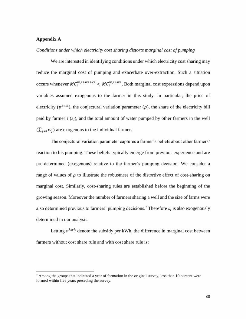
Appendix A

Conditions under which electricity cost sharing distorts marginal cost of pumping

We are interested in identifying conditions under which electricity cost sharing may

reduce the marginal cost of pumping and exacerbate over-extraction. Such a situation

occurs whenever 𝑀𝐶𝑖𝑤,𝑠+𝑤𝑠+𝑐𝑠 < 𝑀𝐶𝑖

𝑤,𝑠+𝑤𝑠. Both marginal cost expressions depend upon

variables assumed exogenous to the farmer in this study. In particular, the price of

electricity (𝑝𝑘𝑤ℎ), the conjectural variation parameter (𝜌), the share of the electricity bill

paid by farmer 𝑖 (𝑠𝑖), and the total amount of water pumped by other farmers in the well

(∑ 𝑤𝑗𝑗≠𝑖 ) are exogenous to the individual farmer.

The conjectural variation parameter captures a farmer’s beliefs about other farmers’

reaction to his pumping. These beliefs typically emerge from previous experience and are

pre-determined (exogenous) relative to the farmer’s pumping decision. We consider a

range of values of 𝜌 to illustrate the robustness of the distortive effect of cost-sharing on

marginal cost. Similarly, cost-sharing rules are established before the beginning of the

growing season. Moreover the number of farmers sharing a well and the size of farms were

also determined previous to farmers’ pumping decisions.7 Therefore 𝑠𝑖 is also exogenously

determined in our analysis.

Letting 𝑣𝑘𝑤ℎ denote the subsidy per kWh, the difference in marginal cost between

farmers without cost share rule and with cost share rule is:

7 Among the groups that indicated a year of formation in the original survey, less than 10 percent were

formed within five years preceding the survey.

39

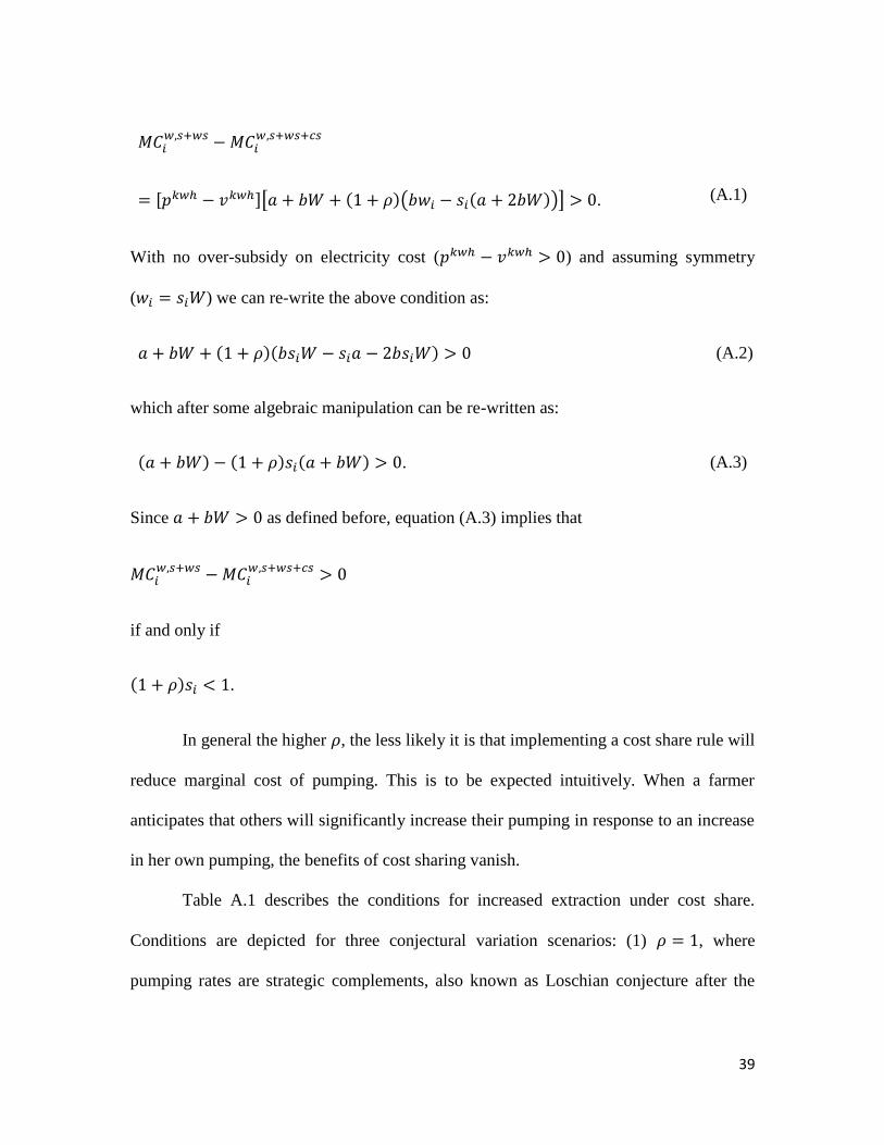
𝑀𝐶𝑖𝑤,𝑠+𝑤𝑠 − 𝑀𝐶𝑖

𝑤,𝑠+𝑤𝑠+𝑐𝑠

= [𝑝𝑘𝑤ℎ − 𝑣𝑘𝑤ℎ][𝑎 + 𝑏𝑊 + (1 + 𝜌)(𝑏𝑤𝑖 − 𝑠𝑖(𝑎 + 2𝑏𝑊))] > 0.

(A.1)

With no over-subsidy on electricity cost (𝑝𝑘𝑤ℎ − 𝑣𝑘𝑤ℎ > 0) and assuming symmetry

(𝑤𝑖 = 𝑠𝑖𝑊) we can re-write the above condition as:

𝑎 + 𝑏𝑊 + (1 + 𝜌)(𝑏𝑠𝑖𝑊 − 𝑠𝑖𝑎 − 2𝑏𝑠𝑖𝑊) > 0 (A.2)

which after some algebraic manipulation can be re-written as:

(𝑎 + 𝑏𝑊) − (1 + 𝜌)𝑠𝑖(𝑎 + 𝑏𝑊) > 0. (A.3)

Since 𝑎 + 𝑏𝑊 > 0 as defined before, equation (A.3) implies that

𝑀𝐶𝑖𝑤,𝑠+𝑤𝑠 − 𝑀𝐶𝑖

𝑤,𝑠+𝑤𝑠+𝑐𝑠 > 0

if and only if

(1 + 𝜌)𝑠𝑖 < 1.

In general the higher 𝜌, the less likely it is that implementing a cost share rule will

reduce marginal cost of pumping. This is to be expected intuitively. When a farmer

anticipates that others will significantly increase their pumping in response to an increase

in her own pumping, the benefits of cost sharing vanish.

Table A.1 describes the conditions for increased extraction under cost share.

Conditions are depicted for three conjectural variation scenarios: (1) 𝜌 = 1, where

pumping rates are strategic complements, also known as Loschian conjecture after the

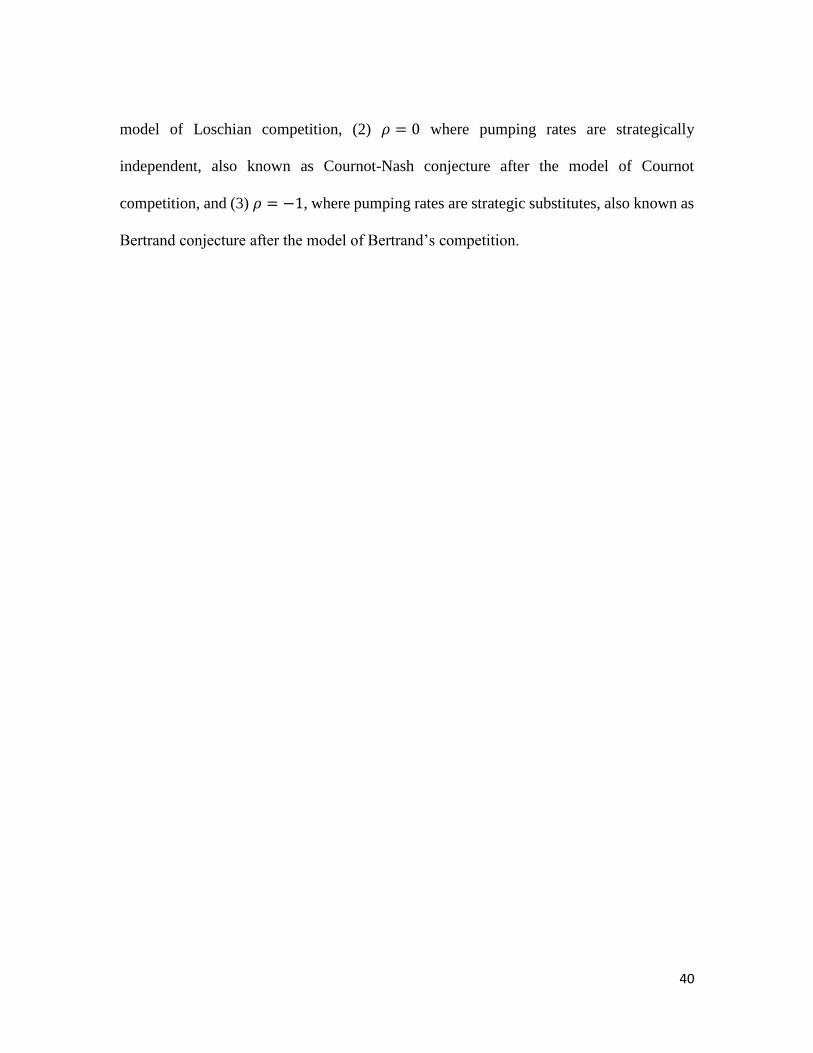
40

model of Loschian competition, (2) 𝜌 = 0 where pumping rates are strategically

independent, also known as Cournot-Nash conjecture after the model of Cournot

competition, and (3) 𝜌 = −1, where pumping rates are strategic substitutes, also known as

Bertrand conjecture after the model of Bertrand’s competition.

41

Table A.1. Marginal cost change under cost share rules

𝑀𝐶𝑖𝑤,𝑠+𝑤𝑠

− 𝑀𝐶𝑖𝑤,𝑠+𝑤𝑠+𝑐𝑠

> 0

𝜌 = −1 [𝑝𝑘𝑤ℎ − 𝑣𝑘𝑤ℎ](𝑎 + 𝑏𝑊) > 0 , which is always true.

𝜌 = 0

[𝑝𝑘𝑤ℎ − 𝑣𝑘𝑤ℎ](𝑎 + 𝑏𝑊)(1 − 𝑠𝑖) > 0 , which holds whenever 𝑠𝑖 < 1. Regardless

of the cost share rule, the condition 𝑠𝑖 < 1 holds for all wells shared by more than one

producer.

𝜌 = 1

[𝑝𝑘𝑤ℎ − 𝑣𝑘𝑤ℎ](𝑎 + 𝑏𝑊)(1 − 2𝑠𝑖) > 0 , which holds whenever 𝑠𝑖 < 0.5. When

costs are evenly split, 𝑠𝑖 < 0.5 holds whenever N>2. When costs are divided based on

land area, 𝑠𝑖 < 0.5 holds for all irrigators that operate less than half of the land

irrigated by the well; i.e. 𝐿𝑖 < 0.5𝐿.

42

Appendix B

Data collection process

The data collection process required two steps. First the enumerators collected the

data on the irrigation unit, (e.g., number of farmers sharing the well, crops grown by

producers) from an individual familiar with the management of the well. In some cases the

respondent is a single individual with well management responsibility while in other cases

it is any one of the users or a group of users. The enumerators then asked the respondent(s)

to identify a representative individual who produced each of the main crops for the unit.

Those identified individuals were interviewed for the crop-specific survey, which was

completed for each of the primary crops grown by producers who share the well. Thus,

there is one crop-specific survey for each crop-well combination. The crop-specific survey

includes questions about inputs, outputs, and prices for each crop.

Cross sectional data was obtained from farmers in a sample of 256 wells. A total of

197 observations contained complete information for our estimation purposes so this is the

size of our sample. Irrigation wells are uniformly scattered across the country so they are

geographically representative of agricultural groundwater irrigators in Mexico. Regarding

the well selection mechanism, a sample was initially drawn based on a national survey of

irrigation wells, and the enumerators tried to find those wells from the sample. However,

in many cases the irrigation wells that were chosen did not exist. In those cases the

enumerators tried to replace the sample well with another well from the same area.

43

Appendix C

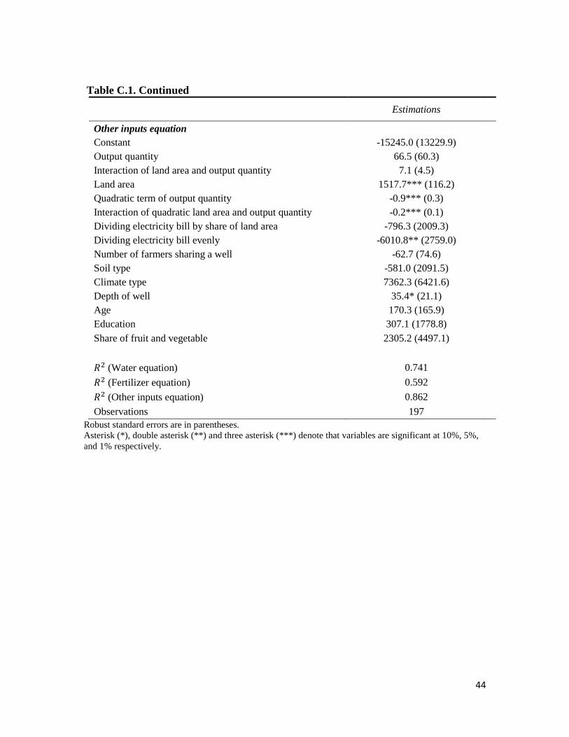
Table C.1. Coefficient Estimates for Input Demands (water, fertilizer and others)

Estimations

Water equation

Constant -39896.6 (33315.0)

Output quantity 547.6** (247.6)

Interaction of land area and output quantity -97.5*** (35.4)

Land area 3208.5*** (394.9)

Quadratic term of output quantity 2.1** (0.9)

Interaction of quadratic land area and output quantity 1.0** (0.5)

Dividing electricity bill by share of land area 16456.9** (8114.8)

Dividing electricity bill evenly 25801.5*** (8515.8)

Number of farmers sharing a well 279.0 (316.5)

Soil type 6566.6 (5629.1)

Climate type 12315.7 (14850.1)

Depth of well 42.8 (54.8)

Age -227.6 (419.2)

Education 4078.8 (4436.3)

Share of fruit and vegetable 3834.3 (11379.4)

Own price elasticity of water -0.06** (0.03)

Fertilizer equation

Constant 2059.1 (8825.2)

Output quantity -167.5** (66.2)

Interaction of land area and output quantity 8.3* (4.9)

Land area 417.3*** (96.9)

Quadratic term of output quantity 0.2 (0.2)

Interaction of quadratic land area and output quantity -0.04 (0.07)

Dividing electricity bill by share of land area -73.9 (1862.8)

Dividing electricity bill evenly -154.4 (2643.8)

Number of farmers sharing a well 62.7 (96.0)

Soil type 358.1 (855.8)

Climate type -7899.0 (5075.5)

Depth of well 2.0 (7.1)

Age 62.9 (71.9)

Education -530.0 (1352.6)

Share of fruit and vegetable 3007.5 (3707.5)

44

Table C.1. Continued

Estimations

Other inputs equation

Constant -15245.0 (13229.9)

Output quantity 66.5 (60.3)

Interaction of land area and output quantity 7.1 (4.5)

Land area 1517.7*** (116.2)

Quadratic term of output quantity -0.9*** (0.3)

Interaction of quadratic land area and output quantity -0.2*** (0.1)

Dividing electricity bill by share of land area -796.3 (2009.3)

Dividing electricity bill evenly -6010.8** (2759.0)

Number of farmers sharing a well -62.7 (74.6)

Soil type -581.0 (2091.5)

Climate type 7362.3 (6421.6)

Depth of well 35.4* (21.1)

Age 170.3 (165.9)

Education 307.1 (1778.8)

Share of fruit and vegetable 2305.2 (4497.1)

𝑅2 (Water equation) 0.741

𝑅2 (Fertilizer equation) 0.592

𝑅2 (Other inputs equation) 0.862

Observations 197

Robust standard errors are in parentheses.

Asterisk (*), double asterisk (**) and three asterisk (***) denote that variables are significant at 10%, 5%,

and 1% respectively.