Embed Size (px)
Citation preview
The Role of Labor Market in Explaining Growth and Inequality:
The Philippines Case♣
Hyun H. Son♠
Economic and Research Department
Asian Development Bank
Abstract: This paper analyzes the relationship between growth and inequality in
the Philippines, focusing on the role played by the labor market. It proposes a
decomposition methodology that explores linkages between growth and labor
market performances in terms of labor force participation, employment, working
hours and productivity. This paper introduces a methodology that provides a
direct linkage between growth, inequality and labor market characteristics. The
paper provides empirical analysis using both the Family Income and Expenditure
Survey (FIES) and Labor Force Survey (LFS), covering the period 1997 to 2003.
♣ This paper is prepared for the 45th Annual Meeting of the Philippine Economic Society on November 14-16, 2007. ♠ The author would like to thank Professor Nanak Kakwani and Jane Carangal-San Jose for their valuable and insightful comments and suggestions on the paper. Email address for correspondence: [email protected]; Tel: 63-2-632 6477; Fax: 63-2-636 2365.
2
1. Introduction
The Philippines has lost its advantage as a developing country that once had a
very promising future in the region to become a highly successful, high growth
economy. This paper posits that the sluggish performance in the growth of jobs
may have contributed to the unimpressive record in economic growth. Along with
low growth, the Philippines has had a persistently high level of income inequality
in the past.
Given a rapid population growth and the high rise in labor force participation,
employment growth in the Philippines has not been sustained at a level that is
sufficient to lower the unemployment and underemployment rate. Productivity
growth has been meager and spotty. Labor productivity increased by less than
7% in the 1988-2000 period in the Philippines, far lower than the increases of 30-
50% in other Asian countries such as Indonesia, Malaysia, Thailand and South
Korea.
Labor income is the main source of people’s income. Labor incomes are
generated through employment in the labor market. Thus, growth in income
depends on the magnitude of employment growth. Nevertheless, employment is
not the only factor that explains labor income. There are other factors that
contribute to labor income. For instance, labor productivity is another factor that
is important in explaining labor income. Labor productivity differs across
individuals and similarly, their access to employment opportunities also varies.
Therefore, the labor market plays a critical role in explaining how much income
people enjoy on average and how their incomes are distributed across
individuals within a country at a given point in time. In this paper, the role of the
labor market is examined in the context of the Philippines.
The main objective of this paper is to analyze economic growth and income
inequality, focusing on the role played by the labor market. It proposes a
3
decomposition methodology that explores the linkages between growth and
income inequality through characteristics such as labor force participation,
employment rate, working hours and productivity. In the literature, the linkage
has often been explored using regression models. Unlike convention however,
this paper examines the direct linkage between growth, inequality and labor
market using a decomposition method.
A corollary objective of this paper is to examine how the Philippine educational
system has addressed the needs of its labor market. The paper deems such an
analysis falls within the purview of gaining a better understanding of how the
labor market has affected the Philippine’s surreal economic performance.
This paper utilizes two sources of data, both of which are denoted as micro unit
record. The data sources are Family Income and Expenditure Survey (FIES) and
Labor Force Survey (LFS). These surveys are undertaken by the Philippine
government’s primary statistical agency, the National Statistics Office (NSO).
The surveys used in this study are for the latest three periods, covering from
1997 to 2003. Moreover, the study uses the merged data sets of FIES and LFS
for the periods of 1997, 2000 and 2003.
The paper is organized in the following manner. Section 2 is devoted to
explaining growth by factor income components. Section 3 investigates the
impact of factor incomes on inequality. While Section 4 looks into trends in key
labor market indicators, Section 5 provides a linkage between growth and labor
market characteristics. Section 6 studies inequities in key labor indicators and
Section 7 is concerned with explaining inequality in labor income. Section 8
provides discussions on the issues of education and labor market and the
following section concludes the study.
4
2. Explaining Growth by Factor Components
GDP per capita and related aggregate income measures are widely used to
assess the economic performance of countries. Economic growth that measures
the rate of change in per capita real GDP has become a standard economic
indicator. Despite the popularity of economic growth as a measure of success,
there is increasing recognition that it is an inadequate measure of a population’s
average well-being. Higher economic growth does not necessarily mean a higher
level of average well-being of the people. This is because GDP includes many
components, which provide disutility to individuals.
Information on incomes of households is now widely available from household
surveys that are conducted by many countries. Given a household size, we
calculate per capita household income for each household. By aggregating per
capita income of each household in the survey, we are able to calculate the
average household income as well as its inequality using an appropriate
inequality measure. In this paper, growth and inequality are analyzed based on
household incomes, which every member of the household actually receives
from various sources.
Suppose x is the total per capita income of a household, which can be written as
the sum of several factor incomes or income components:
∑=
=k
jjxx
1 (1)
where k is the total number of income components and jx is the per capita
income from the jth income component. In our empirical analysis, we have six
income components:
- Agricultural wage income
- Non-agricultural wage income
- Enterprise income
5
- Domestic remittances
- Foreign remittances
- Other residual income (e.g. interest, dividends, pensions, rents etc.)
Suppose μ is the per capita average income of all households in the Philippines
and jμ is the per capita income from the ith income component, then using (1)
we can write
∑=
=k
jj
1μμ (2)
μμ /j is the share of jth income component. This share is useful as it indicates
from which sources households derive their income. Poor households may differ
from the other households with respect to their sources of income. Table 1 shows
where all households and the poor households derive their incomes. It also
shows trends in average per capita income for three years 1997, 2000 and 2003.
Table 1 shows that the share of wages (both agriculture and non-agriculture) in
per capita total household income has been the largest but has declined steadily
from 46.1% in 1997 to 44.8% in 2003. Meanwhile, the share of remittances –
particularly foreign remittances – rose over the period from 9% in 1997 to 12.7%
in 2003. This suggests that remittances have become an important source of
household income in the Philippine economy. As would be expected, remittances
played a significant role as a form of informal safety nets for average households
during the crisis period (1997-2000).
The story is somewhat different for poor households. First of all, a major source
of income for the poor is derived from enterprise activities, not from wages. This
suggests that poor households are mainly working in the informal sector. The
trend in the share of enterprise income to the total income of the poor has fallen
steadily.
6
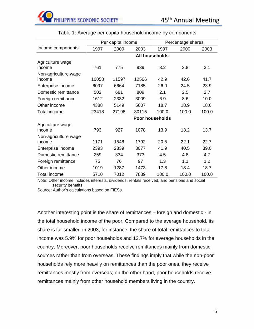
Table 1: Average per capita household income by components
Per capita income Percentage shares Income components 1997 2000 2003 1997 2000 2003
All households Agriculture wage income 761 775 939 3.2 2.8 3.1 Non-agriculture wage income 10058 11597 12566 42.9 42.6 41.7 Enterprise income 6097 6664 7185 26.0 24.5 23.9 Domestic remittance 502 681 809 2.1 2.5 2.7 Foreign remittance 1612 2332 3009 6.9 8.6 10.0 Other income 4388 5149 5607 18.7 18.9 18.6 Total income 23418 27198 30115 100.0 100.0 100.0
Poor households Agriculture wage income 793 927 1078 13.9 13.2 13.7 Non-agriculture wage income 1171 1548 1792 20.5 22.1 22.7 Enterprise income 2393 2839 3077 41.9 40.5 39.0 Domestic remittance 259 334 373 4.5 4.8 4.7 Foreign remittance 75 76 97 1.3 1.1 1.2 Other income 1019 1287 1473 17.8 18.4 18.7 Total income 5710 7012 7889 100.0 100.0 100.0 Note: Other income includes interests, dividends, rentals received, and pensions and social security benefits. Source: Author’s calculations based on FIESs.
Another interesting point is the share of remittances – foreign and domestic - in
the total household income of the poor. Compared to the average household, its
share is far smaller: in 2003, for instance, the share of total remittances to total
income was 5.9% for poor households and 12.7% for average households in the
country. Moreover, poor households receive remittances mainly from domestic
sources rather than from overseas. These findings imply that while the non-poor
households rely more heavily on remittances than the poor ones, they receive
remittances mostly from overseas; on the other hand, poor households receive
remittances mainly from other household members living in the country.
7
We now extend the analysis to examine growth rates and relative contributions of
each income component to the growth in total household income. To do so, each
income component is deflated by the per capita poverty line which takes into
account the differences in regional costs of living as well as changes in prices
over time. Doing so gives us average per capita welfare. Having made the
adjustment for the prices, we can calculate the growth rate of per capital total
income and individual income components. It is useful to know how much each
income source contributes to the growth in total income.
Suppose r is the growth rate of per capita total real income and jr is the growth
rate of per capita real jth income component, then using (2), we can write
∑=
=k
jjj rr
1)/( μμ (3)
which shows that the growth rate of total income is equal to the weighted
average of the growth rates of the individual income components, where weight
is given by the share of each income component. jj r)/( μμ is the contribution of
the jth income component to the growth rate of total income.
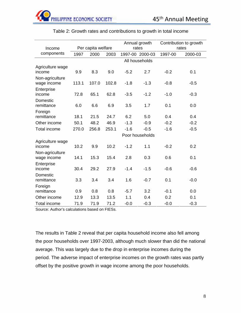
As shown in Table 2, per capita total household income has declined over 1997-
2003. As would be expected, the fall was particularly greater during the crisis
period. Over 1997-2000, components such as wages and enterprise income fell
sharply but domestic and foreign remittances grew at an annual rate of 3.5% and
6.2%, respectively. These findings suggest, thus, that the fall in per capita total
income could have been much greater in the absence of any remittances,
particularly from migrant workers. This is also indicated by the positive relative
contribution of the growth in remittances, to the growth in total household income.
Other components – particularly non-agricultural wages and enterprise income –
have been largely responsible for the negative growth in the total income over
the period.
8
Table 2: Growth rates and contributions to growth in total income
Per capita welfare Annual growth
rates Contribution to growth
rates Income components 1997 2000 2003 1997-00 2000-03 1997-00 2000-03
All households Agriculture wage income 9.9 8.3 9.0 -5.2 2.7 -0.2 0.1 Non-agriculture wage income 113.1 107.0 102.8 -1.8 -1.3 -0.8 -0.5 Enterprise income 72.8 65.1 62.8 -3.5 -1.2 -1.0 -0.3 Domestic remittance 6.0 6.6 6.9 3.5 1.7 0.1 0.0 Foreign remittance 18.1 21.5 24.7 6.2 5.0 0.4 0.4 Other income 50.1 48.2 46.9 -1.3 -0.9 -0.2 -0.2 Total income 270.0 256.8 253.1 -1.6 -0.5 -1.6 -0.5
Poor households Agriculture wage income 10.2 9.9 10.2 -1.2 1.1 -0.2 0.2 Non-agriculture wage income 14.1 15.3 15.4 2.8 0.3 0.6 0.1 Enterprise income 30.4 29.2 27.9 -1.4 -1.5 -0.6 -0.6 Domestic remittance 3.3 3.4 3.4 1.6 -0.7 0.1 -0.0 Foreign remittance 0.9 0.8 0.8 -5.7 3.2 -0.1 0.0 Other income 12.9 13.3 13.5 1.1 0.4 0.2 0.1 Total income 71.9 71.9 71.2 -0.0 -0.3 -0.0 -0.3 Source: Author’s calculations based on FIESs.
The results in Table 2 reveal that per capita household income also fell among
the poor households over 1997-2003, although much slower than did the national
average. This was largely due to the drop in enterprise incomes during the
period. The adverse impact of enterprise incomes on the growth rates was partly
offset by the positive growth in wage income among the poor households.
9
In recapping, Filipino households derive their incomes mainly from labor incomes
with the poor being more reliant on enterprise earnings. While remittances
buffered incomes during the crisis years, foreign remittances flowed mostly to the
non-poor while the poor tend to rely more on domestic remittances.
3. Impact of Factor Incomes on Inequality
In view of its diversity, the Philippines became divided into 16 distinct regions. A
major problem in the country is the regional disparity in living conditions.
Disparity can be very large even within regions. Any analysis of inequality should
reflect such regional variations. Theil’s measure of inequality is well suited to
analyze inequality in the Philippines because it can be decomposed into
between- and within-regional inequality. In this section, we use the Theil’s index
to explain how inequality in total income is impacted by changes in factor
incomes.
Suppose x is the per capita total household income, which is a random variable
with density function f(x), then Theil’s inequality measure can be written as
[ ]∫∝
−=0
)()log()log( dxxfxT μ (4)
The question we want to address is: how does growth in factor incomes affect
inequality? For example, we want to know how foreign transfers to recipient
households affect inequality in per capita total income. If increases in foreign
transfers increase inequality, we can conclude that foreign transfers are anti-poor
because they benefit the non-poor proportionally more than the poor. Similarly, if
these transfers reduce inequality, then it can be said that they are pro-poor
benefiting the poor more than the non-poor. From a policy point of view, it is
important to know which income components are pro-poor or anti-poor. These
questions can be answered by means of the elasticity of inequality with respect
to the various income components.

10
The elasticity of Theil’s inequality measure T in (4) with respect to jμ can be
written as
∫∞
⎥⎦
⎤⎢⎣
⎡−=
∂∂
=0
)(1 dxxfxx
TT
Tjj
j
jj μ
μμ
μη (5)
which tells us that if jμ increases by 1%, the inequality measure T will change by
jη %. If jμ is negative (positive), this implies that a growth in the jth income
component will decrease (increase) the inequality of per capita total income.
Thus, the jth income component is pro-poor (anti-poor) if jμ is negative
(positive). It can be easily verified that 01
=∑=
k
jjη , implying that when all income
components increase by 1%, total inequality does not change.
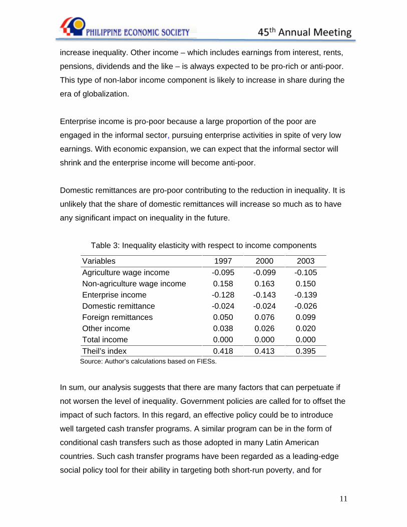
Table 3 presents the inequality elasticity with respect to the various income
components. The components that would result in a reduction in inequality are:
agricultural wage income, enterprise income and domestic remittances. Those
that would that increase inequality are: non-agricultural wage income, foreign
remittances and other income. These have important implications. First, the
agricultural wage income is pro-poor in the sense that it has contributed to a
reduction in inequality. Yet since its share has been declining over time, we can
expect that the on-going transformation of the economic structure will continue to
worsen inequality in future. Second, the share of the non-agricultural wage
income, from which the households derive a major source of livelihood, will
continue to increase. Thus, it would be expected that the increasing share of
non-agricultural wage income in the total household income will be a major factor
that contributes to the increase in inequality.
As we have noted earlier, foreign remittances have contributed significantly to the
growth in total household income. Unfortunately, this component tends to
11
increase inequality. Other income – which includes earnings from interest, rents,
pensions, dividends and the like – is always expected to be pro-rich or anti-poor.
This type of non-labor income component is likely to increase in share during the
era of globalization.
Enterprise income is pro-poor because a large proportion of the poor are
engaged in the informal sector, pursuing enterprise activities in spite of very low
earnings. With economic expansion, we can expect that the informal sector will
shrink and the enterprise income will become anti-poor.
Domestic remittances are pro-poor contributing to the reduction in inequality. It is
unlikely that the share of domestic remittances will increase so much as to have
any significant impact on inequality in the future.
Table 3: Inequality elasticity with respect to income components
Variables 1997 2000 2003 Agriculture wage income -0.095 -0.099 -0.105 Non-agriculture wage income 0.158 0.163 0.150 Enterprise income -0.128 -0.143 -0.139 Domestic remittance -0.024 -0.024 -0.026 Foreign remittances 0.050 0.076 0.099 Other income 0.038 0.026 0.020 Total income 0.000 0.000 0.000 Theil’s index 0.418 0.413 0.395
Source: Author’s calculations based on FIESs.
In sum, our analysis suggests that there are many factors that can perpetuate if
not worsen the level of inequality. Government policies are called for to offset the
impact of such factors. In this regard, an effective policy could be to introduce
well targeted cash transfer programs. A similar program can be in the form of
conditional cash transfers such as those adopted in many Latin American
countries. Such cash transfer programs have been regarded as a leading-edge
social policy tool for their ability in targeting both short-run poverty, and for
12
improving the human capital of the poor. In addition, these programs have been
lauded for their ability to focus on the poor, for making it easier to integrate
different types of social service (e.g. education, health and nutrition), and for their
cost-effectiveness performance.
4. Labor Market Indicators
As discussed earlier, the average Filipino household derives its major source of
income from labor earnings. Table 1 shows that more than 70% of total
household income is generated from labor earnings. This implies the enormous
impact that the labor market has on both growth and changes in inequality. In this
section, we discuss the trends of a few key indicators of the labor market.
These indicators are normally defined in terms of individual characteristics, while
growth and inequality measures are estimated from household characteristics. A
question then arises as to how such different characteristics of households and
individuals could be linked. An initial step to address this issue is by converting
individual labor market indicators into household indicators. This represents an
important contribution of the paper to studies in this area that attempt to link labor
market with growth and inequality. For instance, per capita employment in a
household is obtained by the total number of employed persons in a household
divided by the household size. From Table 4, average per capita employment
within households was calculated as equal to 0.384 in 2003. This means that on
average, about 38.4% of household members were employed in 2003: almost 2
members living in a 5-member household were engaged in some form of
employment in the labor market.
In Table 4, we present five labor market indicators for households:
- Per capita employment: (e )
- Per capita unemployment: (u )
- Per capita labor force participation rate (LFP): ( uel += )
- Per capita work hours: (h )
13
- Per capita labor income: ( lx for nominal and *lx for real)
Using these indicators, we can define:
- Employment rate: ⎟⎠⎞
⎜⎝⎛
le
- Work hours per employed person: ⎟⎠⎞
⎜⎝⎛
eh
- Labor productivity: ⎟⎠⎞
⎜⎝⎛
hxl for nominal and ⎟⎟
⎠
⎞⎜⎜⎝
⎛hxl
*
for real
The labor force participation rate for a household is defined as the sum of per
capita employment and per capita unemployment; the employment rate in a
household is measured by per capita employment divided by per capita labor
force participation rate; work hour per employed person is obtained by per capita
work hours divided by per capita employment.
In addition, labor productivity for each household is defined as per capita labor
earnings divided by per capita work hours. Labor productivity can be expressed
in both nominal and real terms. To examine trends in labor productivity, labor
earnings should be adjusted for prices. Thus, the real productivity is equal to
nominal productivity adjusted for prices.
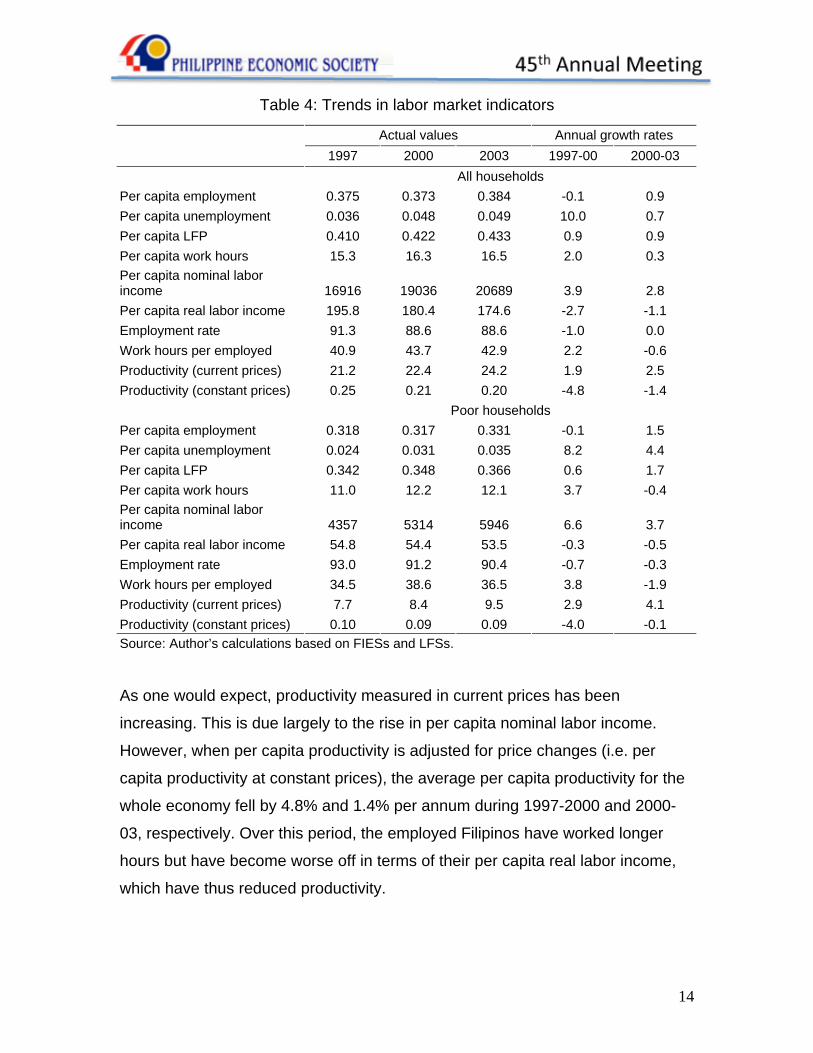
Table 4 shows a number of points that merit emphasis. Per capita employment
has increased from 0.375 in 1997 to 0.384 in 2003, but this has not been
sufficient to lower per capita unemployment given a rise in the LFP in the
economy. LFP grew at an annual rate of 0.9% while per capita unemployment
jumped by 10% per annum during the crisis period and increased by slightly less
than 1% annually afterwards. This meant that the number of jobs available in the
labor market has not grown fast enough to absorb the number of new entrants to
the labor force. This can be similarly observed for poor households.
14
Table 4: Trends in labor market indicators
Actual values Annual growth rates 1997 2000 2003 1997-00 2000-03 All households
Per capita employment 0.375 0.373 0.384 -0.1 0.9 Per capita unemployment 0.036 0.048 0.049 10.0 0.7 Per capita LFP 0.410 0.422 0.433 0.9 0.9 Per capita work hours 15.3 16.3 16.5 2.0 0.3 Per capita nominal labor income 16916 19036 20689 3.9 2.8 Per capita real labor income 195.8 180.4 174.6 -2.7 -1.1 Employment rate 91.3 88.6 88.6 -1.0 0.0 Work hours per employed 40.9 43.7 42.9 2.2 -0.6 Productivity (current prices) 21.2 22.4 24.2 1.9 2.5 Productivity (constant prices) 0.25 0.21 0.20 -4.8 -1.4
Poor households Per capita employment 0.318 0.317 0.331 -0.1 1.5 Per capita unemployment 0.024 0.031 0.035 8.2 4.4 Per capita LFP 0.342 0.348 0.366 0.6 1.7 Per capita work hours 11.0 12.2 12.1 3.7 -0.4 Per capita nominal labor income 4357 5314 5946 6.6 3.7 Per capita real labor income 54.8 54.4 53.5 -0.3 -0.5 Employment rate 93.0 91.2 90.4 -0.7 -0.3 Work hours per employed 34.5 38.6 36.5 3.8 -1.9 Productivity (current prices) 7.7 8.4 9.5 2.9 4.1 Productivity (constant prices) 0.10 0.09 0.09 -4.0 -0.1 Source: Author’s calculations based on FIESs and LFSs.
As one would expect, productivity measured in current prices has been
increasing. This is due largely to the rise in per capita nominal labor income.
However, when per capita productivity is adjusted for price changes (i.e. per
capita productivity at constant prices), the average per capita productivity for the
whole economy fell by 4.8% and 1.4% per annum during 1997-2000 and 2000-
03, respectively. Over this period, the employed Filipinos have worked longer
hours but have become worse off in terms of their per capita real labor income,
which have thus reduced productivity.
15
5. Linking Growth with Labor Market Characteristics This section attempts to explain how changes in certain labor market
characteristics, contribute to the growth in per capita real labor income. Using the
definitions in Section 4, we can express the logarithm of average per capita real
labor income as
)/()/()/()()( ** hxLnehLnleLnlLnxLn ll +++= (6)
where bars on variables indicate the average over all households. For instance, *lx is the average per capita real labor income. If we take the first difference in
(6), we obtain the growth rates. Thus, the growth rate of per capita real labor
income can be expressed as the sum of the contributions by the following four
factors:
- Average labor force participation rate
- Average employment rate
- Average work hours per employed person
- Average labor productivity
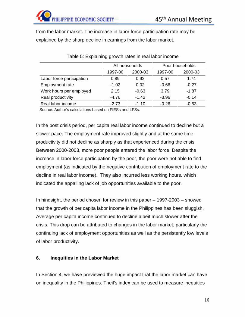
These four contributions are quantified for all households as well as for poor
households in Table 5. The per capita labor income declined at an annual rate of
2.73% between 1997 and 2000, stemming from the deep economic crisis in Asia.
What are the factors that have contributed to this decline? The employment rate
contributed to reduction in growth rate by 1.02%. Despite a fall in employment
rate, the employed persons worked more hours, which contributed to a positive
growth rate of 2.15%. It appears that during the crisis, those who were employed
had to work longer hours because their hourly earnings were falling rapidly. This
drop in earnings is reflected by the negative contribution of real productivity to
growth of 4.76%. Interestingly, there was an increase in labor force participation
rate, which made a positive contribution growth rate by 0.89%. Generally when
the labor market is weak, many workers particularly women tend to withdraw
16
from the labor market. The increase in labor force participation rate may be
explained by the sharp decline in earnings from the labor market.
Table 5: Explaining growth rates in real labor income
All households Poor households 1997-00 2000-03 1997-00 2000-03
Labor force participation 0.89 0.92 0.57 1.74 Employment rate -1.02 0.02 -0.66 -0.27 Work hours per employed 2.15 -0.63 3.79 -1.87 Real productivity -4.76 -1.42 -3.96 -0.14 Real labor income -2.73 -1.10 -0.26 -0.53
Source: Author’s calculations based on FIESs and LFSs.
In the post crisis period, per capita real labor income continued to decline but a
slower pace. The employment rate improved slightly and at the same time
productivity did not decline as sharply as that experienced during the crisis.
Between 2000-2003, more poor people entered the labor force. Despite the
increase in labor force participation by the poor, the poor were not able to find
employment (as indicated by the negative contribution of employment rate to the
decline in real labor income). They also incurred less working hours, which
indicated the appalling lack of job opportunities available to the poor.
In hindsight, the period chosen for review in this paper – 1997-2003 – showed
that the growth of per capita labor income in the Philippines has been sluggish.
Average per capita income continued to decline albeit much slower after the
crisis. This drop can be attributed to changes in the labor market, particularly the
continuing lack of employment opportunities as well as the persistently low levels
of labor productivity.
6. Inequities in the Labor Market
In Section 4, we have previewed the huge impact that the labor market can have
on inequality in the Philippines. Theil’s index can be used to measure inequities
17
in the labor market. This index can be calculated for labor market indicators such
as per capita labor force participation rate, per capita employment, per capita
work hours and per capita labor income. For example, the Theil’s index for per
capita employment can be given by
∫ −= dxxfeeT e )()]log()[log()( μ (7)
where eμ is the average per capita employment. T(e) measures the inequality in
employment across individuals belonging to a household.
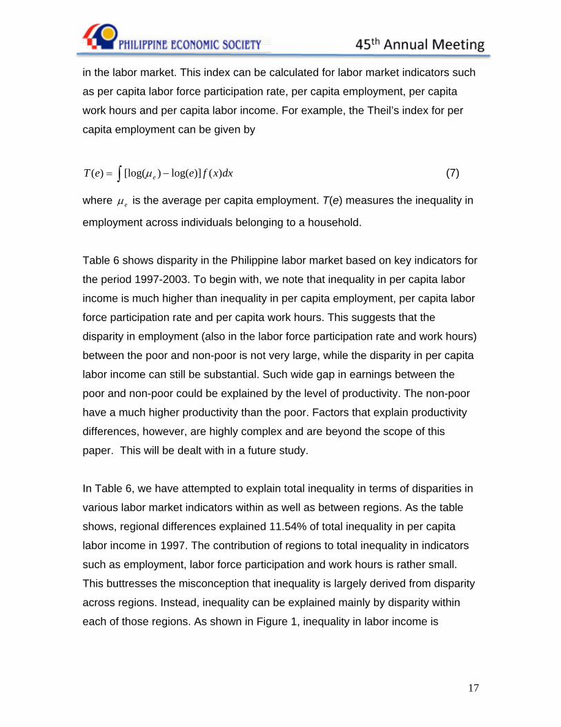
Table 6 shows disparity in the Philippine labor market based on key indicators for
the period 1997-2003. To begin with, we note that inequality in per capita labor
income is much higher than inequality in per capita employment, per capita labor
force participation rate and per capita work hours. This suggests that the
disparity in employment (also in the labor force participation rate and work hours)
between the poor and non-poor is not very large, while the disparity in per capita
labor income can still be substantial. Such wide gap in earnings between the
poor and non-poor could be explained by the level of productivity. The non-poor
have a much higher productivity than the poor. Factors that explain productivity
differences, however, are highly complex and are beyond the scope of this
paper. This will be dealt with in a future study.
In Table 6, we have attempted to explain total inequality in terms of disparities in
various labor market indicators within as well as between regions. As the table
shows, regional differences explained 11.54% of total inequality in per capita
labor income in 1997. The contribution of regions to total inequality in indicators
such as employment, labor force participation and work hours is rather small.
This buttresses the misconception that inequality is largely derived from disparity
across regions. Instead, inequality can be explained mainly by disparity within
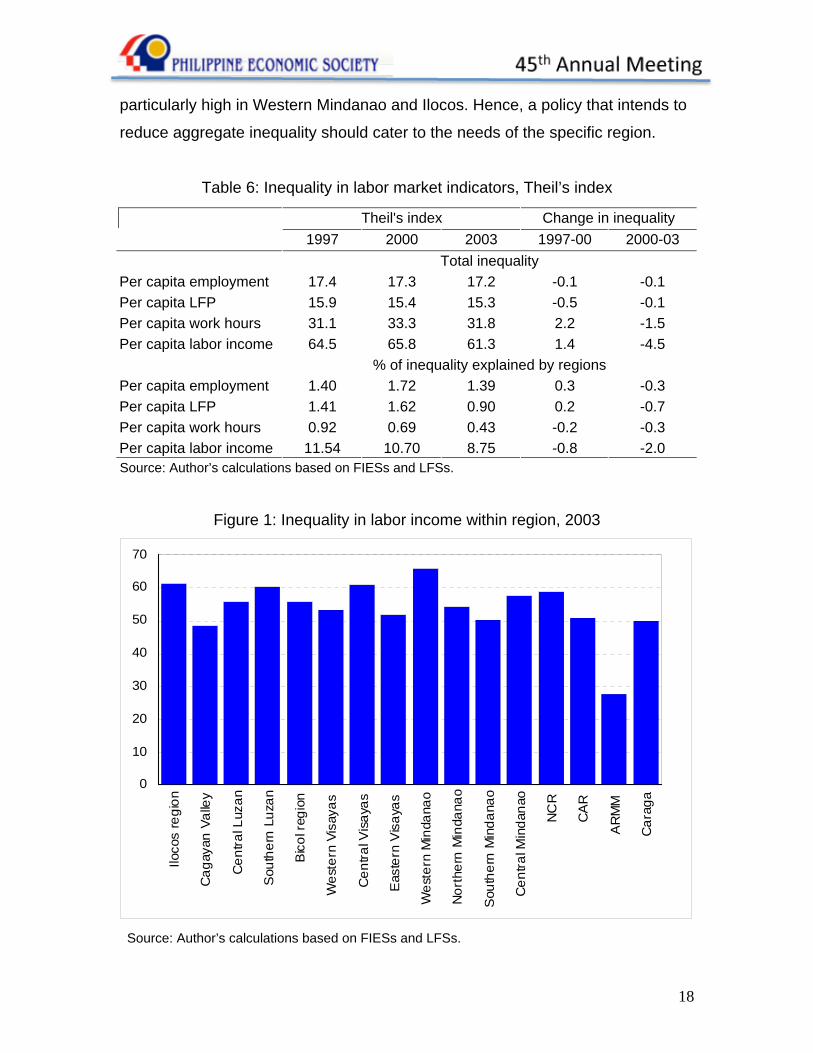
each of those regions. As shown in Figure 1, inequality in labor income is
18
particularly high in Western Mindanao and Ilocos. Hence, a policy that intends to
reduce aggregate inequality should cater to the needs of the specific region.
Table 6: Inequality in labor market indicators, Theil’s index
Theil's index Change in inequality 1997 2000 2003 1997-00 2000-03 Total inequality
Per capita employment 17.4 17.3 17.2 -0.1 -0.1 Per capita LFP 15.9 15.4 15.3 -0.5 -0.1 Per capita work hours 31.1 33.3 31.8 2.2 -1.5 Per capita labor income 64.5 65.8 61.3 1.4 -4.5
% of inequality explained by regions Per capita employment 1.40 1.72 1.39 0.3 -0.3 Per capita LFP 1.41 1.62 0.90 0.2 -0.7 Per capita work hours 0.92 0.69 0.43 -0.2 -0.3 Per capita labor income 11.54 10.70 8.75 -0.8 -2.0 Source: Author’s calculations based on FIESs and LFSs.
Figure 1: Inequality in labor income within region, 2003
Iloco
s re
gion
Cag
ayan
Val
ley
Cen
tral L
uzan
Sou
ther
n Lu
zan
Bic
ol r
egio
n
Wes
tern
Vis
ayas
Cen
tral V
isay
as
Eas
tern
Vis
ayas
Wes
tern
Min
dana
o
Nor
ther
n M
inda
nao
Sou
ther
n M
inda
nao
Cen
tral M
inda
nao
NC
R
CA
R
AR
MM
Car
aga
0
10
20
30
40
50
60
70
Source: Author’s calculations based on FIESs and LFSs.
19
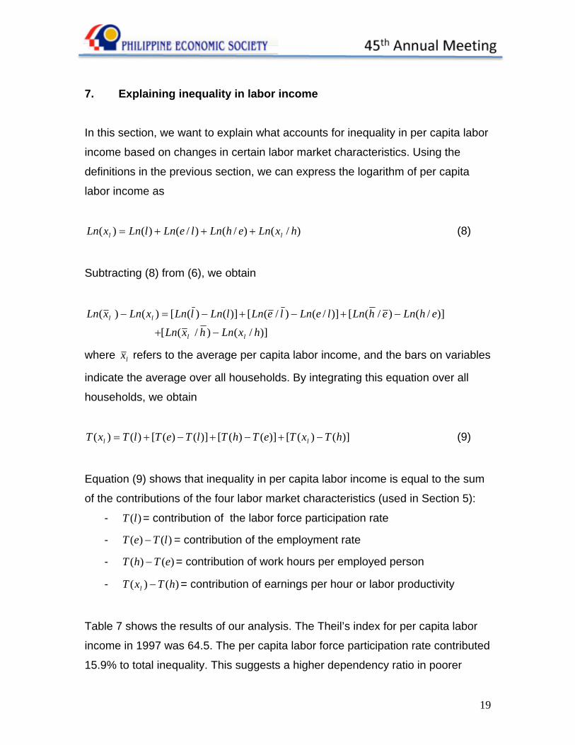
7. Explaining inequality in labor income In this section, we want to explain what accounts for inequality in per capita labor
income based on changes in certain labor market characteristics. Using the
definitions in the previous section, we can express the logarithm of per capita
labor income as
)/()/()/()()( hxLnehLnleLnlLnxLn ll +++= (8)
Subtracting (8) from (6), we obtain
)]/()/([
)]/()/([)]/()/([)]()([)()(
hxLnhxLn
ehLnehLnleLnleLnlLnlLnxLnxLn
ll
ll
−+
−+−+−=−
where lx refers to the average per capita labor income, and the bars on variables
indicate the average over all households. By integrating this equation over all
households, we obtain
)]()([)]()([)]()([)()( hTxTeThTlTeTlTxT ll −+−+−+= (9)
Equation (9) shows that inequality in per capita labor income is equal to the sum
of the contributions of the four labor market characteristics (used in Section 5):
- )(lT = contribution of the labor force participation rate
- )()( lTeT − = contribution of the employment rate
- )()( eThT − = contribution of work hours per employed person
- )()( hTxT l − = contribution of earnings per hour or labor productivity
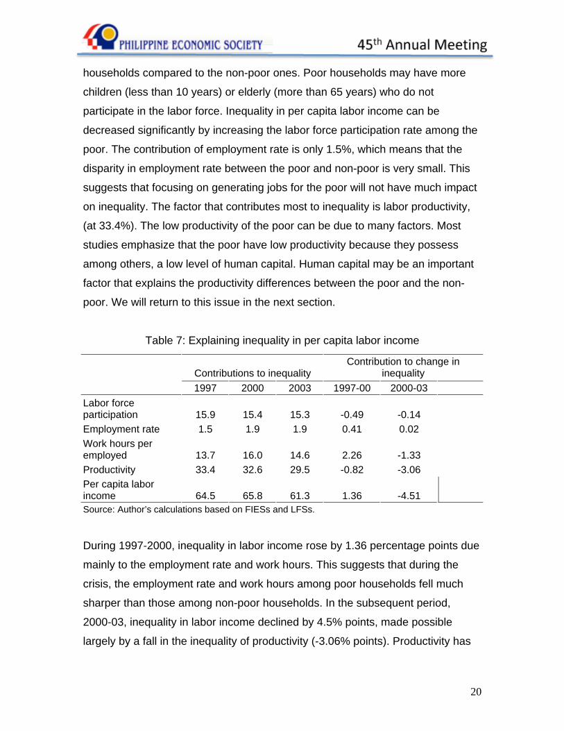
Table 7 shows the results of our analysis. The Theil’s index for per capita labor
income in 1997 was 64.5. The per capita labor force participation rate contributed
15.9% to total inequality. This suggests a higher dependency ratio in poorer
20
households compared to the non-poor ones. Poor households may have more
children (less than 10 years) or elderly (more than 65 years) who do not
participate in the labor force. Inequality in per capita labor income can be
decreased significantly by increasing the labor force participation rate among the
poor. The contribution of employment rate is only 1.5%, which means that the
disparity in employment rate between the poor and non-poor is very small. This
suggests that focusing on generating jobs for the poor will not have much impact
on inequality. The factor that contributes most to inequality is labor productivity,
(at 33.4%). The low productivity of the poor can be due to many factors. Most
studies emphasize that the poor have low productivity because they possess
among others, a low level of human capital. Human capital may be an important
factor that explains the productivity differences between the poor and the non-
poor. We will return to this issue in the next section.
Table 7: Explaining inequality in per capita labor income
Contributions to inequality Contribution to change in
inequality 1997 2000 2003 1997-00 2000-03
Labor force participation 15.9 15.4 15.3 -0.49 -0.14 Employment rate 1.5 1.9 1.9 0.41 0.02 Work hours per employed 13.7 16.0 14.6 2.26 -1.33 Productivity 33.4 32.6 29.5 -0.82 -3.06 Per capita labor income 64.5 65.8 61.3 1.36 -4.51 Source: Author’s calculations based on FIESs and LFSs.
During 1997-2000, inequality in labor income rose by 1.36 percentage points due
mainly to the employment rate and work hours. This suggests that during the
crisis, the employment rate and work hours among poor households fell much
sharper than those among non-poor households. In the subsequent period,
2000-03, inequality in labor income declined by 4.5% points, made possible
largely by a fall in the inequality of productivity (-3.06% points). Productivity has

21
become more equal across households. This is consistent with our earlier finding
that the fall in real productivity was far smaller among the poor than among the
national average. Hence, the gap in productivity difference between the poor and
the non-poor has narrowed down in 2000-03.
In synthesizing how the labor market impacts on inequality in the Philippines, our
findings show that inequality in the Philippine labor market can be attributed to
disparities within each region, rather than across regions. Within each region,
the gaps in per capita incomes are quite pronounced. Moreover, looking closely
at inequality levels within each region, the findings reveal that the level of and
changes in labor productivity can explain much of the disparity in labor incomes.
Similar to growth, labor productivity impacts significantly on inequality in the
Philippines.
8. Education and Labor Market
The previous sections illustrate the importance of labor incomes in influencing
the pattern and trends of growth and inequality in the Philippines. As a corollary
objective, this paper maintains that a discussion of this linkage will be more
complete with a review of how the country’s educational system responds to the
needs of its labor market.
Because households make important decisions on schooling and the choice to
work, it is most logical to use a micro approach to look into the relationship
between education, and labor productivity and earnings. The primary motivations
to attend school are better future income prospects and personal well-being.
Education is known not only to lead to higher earnings but also to other non-labor
market benefits, for instance better nutrition and health, better capacity to enjoy
leisure (Haveman and Wolfe 1984). In line with the human capital view of
education, higher earnings are compensation for increased productivity through
education.
22
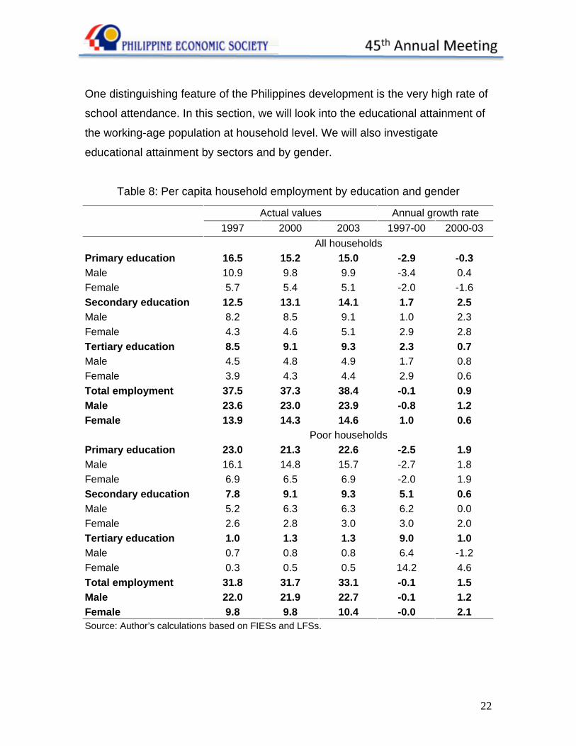
One distinguishing feature of the Philippines development is the very high rate of
school attendance. In this section, we will look into the educational attainment of
the working-age population at household level. We will also investigate
educational attainment by sectors and by gender.
Table 8: Per capita household employment by education and gender
Actual values Annual growth rate 1997 2000 2003 1997-00 2000-03 All households
Primary education 16.5 15.2 15.0 -2.9 -0.3 Male 10.9 9.8 9.9 -3.4 0.4 Female 5.7 5.4 5.1 -2.0 -1.6 Secondary education 12.5 13.1 14.1 1.7 2.5 Male 8.2 8.5 9.1 1.0 2.3 Female 4.3 4.6 5.1 2.9 2.8 Tertiary education 8.5 9.1 9.3 2.3 0.7 Male 4.5 4.8 4.9 1.7 0.8 Female 3.9 4.3 4.4 2.9 0.6 Total employment 37.5 37.3 38.4 -0.1 0.9 Male 23.6 23.0 23.9 -0.8 1.2 Female 13.9 14.3 14.6 1.0 0.6
Poor households Primary education 23.0 21.3 22.6 -2.5 1.9 Male 16.1 14.8 15.7 -2.7 1.8 Female 6.9 6.5 6.9 -2.0 1.9 Secondary education 7.8 9.1 9.3 5.1 0.6 Male 5.2 6.3 6.3 6.2 0.0 Female 2.6 2.8 3.0 3.0 2.0 Tertiary education 1.0 1.3 1.3 9.0 1.0 Male 0.7 0.8 0.8 6.4 -1.2 Female 0.3 0.5 0.5 14.2 4.6 Total employment 31.8 31.7 33.1 -0.1 1.5 Male 22.0 21.9 22.7 -0.1 1.2 Female 9.8 9.8 10.4 -0.0 2.1 Source: Author’s calculations based on FIESs and LFSs.
23
Table 8 shows the educational levels for those employed within households -
both for the average and the poor during the period 1997-2003. To begin with,
one should note that the figures presented in the table are all expressed in per
capita terms within households. For instance, per capita educational level within
households was 38.4% in 2003. This means that on average, about 38.4% of
household members were employed in 2003: almost 2 members living in a 5-
member household were engaged in some form of employment in the labor
market.
Table 8 shows a number of important findings. Per capita employment has
increased from 37.5% in 1997 to 38.4% in 2003, yet this has not been sufficient
to lower per capita unemployment given the rise in labor force participation (LFP)
in the economy. According to our earlier results (see Section 4), per capita LFP
has been growing by 0.9% per annum while per capita unemployment jumped at
10% per annum during the crisis period (1997-2000) and rose slightly by less
than 1% annually afterwards (2000-03). Overall, the number of jobs available in
the labor market has not been growing fast enough to absorb the number of new
entrants to the labor force.
Table 8 also indicates that household members are getting more educated in the
Philippines. Over the period 1997-2003, the proportion of employed household
members who have secondary and tertiary education has increased, while those
who have acquired primary education have declined. This suggests that higher
education matters for employment in the Philippines labor market. Nevertheless,
almost 70% of the employed among the poor households have acquired only
primary education.
In terms of gender, the proportion of employed female members tends to be
higher at secondary and tertiary level. Its growth is quite strong over the period,
particularly among the poor households. Moreover, the gender gap in the
24
employment rate within household narrows down – still higher for male members
– particularly at tertiary level.
Based on the foregoing so far, a puzzle remains as to the differences in the
employability of male and female employed by educational levels. Our study
suggests that educational attainment is higher for women compared to men.
However, it does not seem to be the case that higher educational attainment
among females leads to their greater employability in the labor market. This issue
will be discussed below.
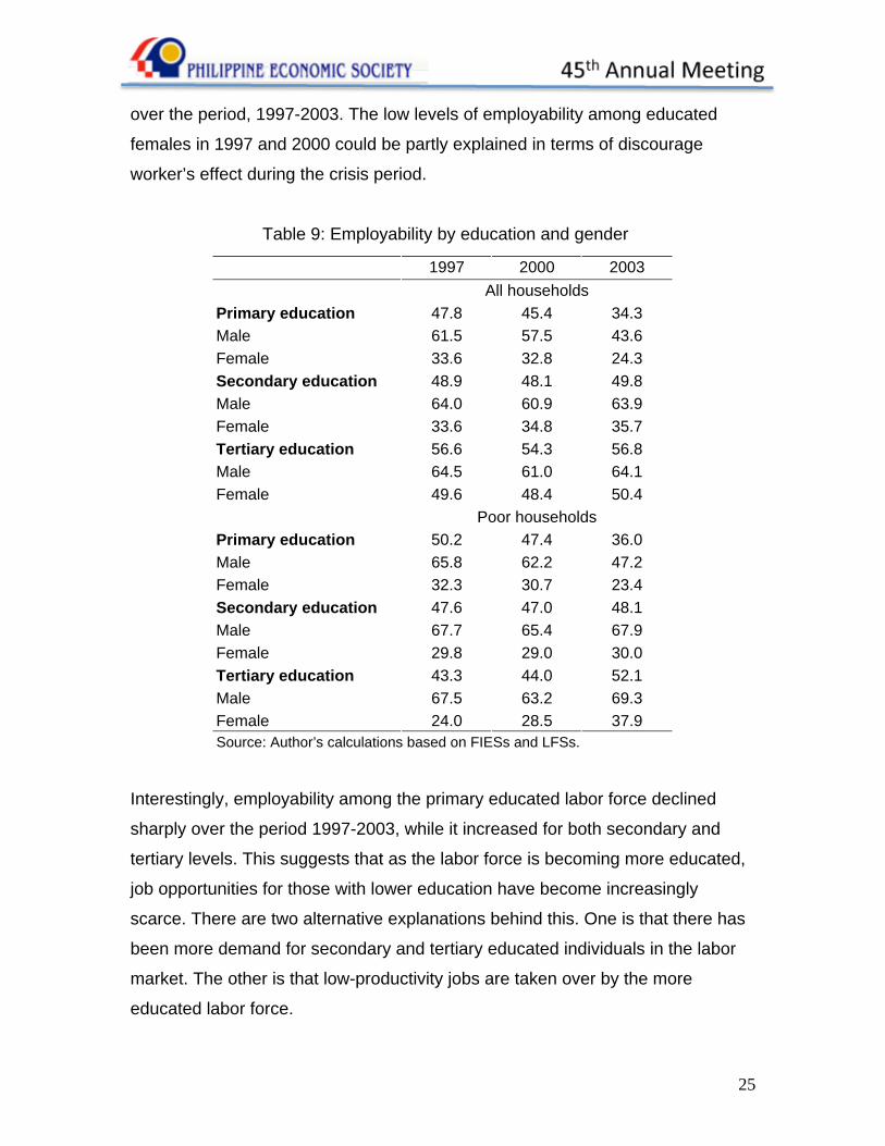
In general, one would expect employability to increase with a higher level of
education. Such a pattern is indeed observed from Table 9. For instance in
1997, employability among the primary educated persons is 47.8%, rising to
48.9% among secondary educated, and reaching 56.6% among the tertiary
educated.
Such a pattern can be observed for average households, but not necessarily for
poor households in 1997 and 2000. This could be because poor households find
work mainly in the informal sector that does not recruit skilled laborers or those
with higher education. This can also be explained by the large unemployability
among the female members of poor households, particularly at tertiary level.
Employability is far greater for male members of poor households compared to
those of average households. This finding is consistent with the view that poor
people cannot afford to be unemployed. More importantly, at all education levels,
women have much lower employability than men. The male-female gap,
however, is much less among those with college education.
Furthermore, it is interesting to note that on average, almost 50% of tertiary
educated females do not work, whereas the corresponding figure for poor
households is more than 60-70%. In addition, employability among tertiary
educated females who belong to the poor households has increased dramatically
25
over the period, 1997-2003. The low levels of employability among educated
females in 1997 and 2000 could be partly explained in terms of discourage
worker’s effect during the crisis period.
Table 9: Employability by education and gender
1997 2000 2003 All households
Primary education 47.8 45.4 34.3 Male 61.5 57.5 43.6 Female 33.6 32.8 24.3 Secondary education 48.9 48.1 49.8 Male 64.0 60.9 63.9 Female 33.6 34.8 35.7 Tertiary education 56.6 54.3 56.8 Male 64.5 61.0 64.1 Female 49.6 48.4 50.4
Poor households Primary education 50.2 47.4 36.0 Male 65.8 62.2 47.2 Female 32.3 30.7 23.4 Secondary education 47.6 47.0 48.1 Male 67.7 65.4 67.9 Female 29.8 29.0 30.0 Tertiary education 43.3 44.0 52.1 Male 67.5 63.2 69.3 Female 24.0 28.5 37.9
Source: Author’s calculations based on FIESs and LFSs.
Interestingly, employability among the primary educated labor force declined
sharply over the period 1997-2003, while it increased for both secondary and
tertiary levels. This suggests that as the labor force is becoming more educated,
job opportunities for those with lower education have become increasingly
scarce. There are two alternative explanations behind this. One is that there has
been more demand for secondary and tertiary educated individuals in the labor
market. The other is that low-productivity jobs are taken over by the more
educated labor force.
26
If the latter is true, the above observations suggest that the labor productivity of
educated workers has been on the decline. As indicated in Table 8, per capita
employment has remained roughly constant over the period. This implies that
employment has increased merely in line with the population growth. Hence, if
there is no improvement in labor productivity, then growth in per capita real labor
earnings is expected to stagnate. To achieve a positive growth, labor productivity
has to increase. Total labor productivity depends on the pattern of employment
by sectors and gender.
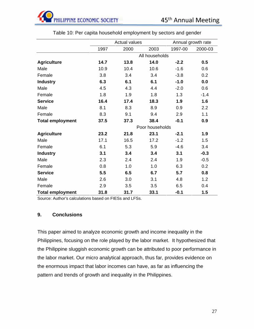
Table 10 shows per capita household employment by sectors and gender.
Accordingly, in terms of magnitudes, the proportion of household members
employed in agriculture has declined, has remained virtually unchanged in the
industrial sector and has risen for the service sector. This suggests a structural
change where the labor force is moving away from the agricultural sector towards
the service sector. Overall, the average household members are largely
employed in services. In the service sector, there is a significant increase in the
employment of female household members over the period. This could be
supported by a claim that the proportion of female college graduates employed in
finance, insurance and real estates has increased over time (Orbeta 2002).
As the findings clearly suggest, the working-age population is increasingly more
engaged in the service sector. Although the service sector tends to create more
number of jobs, the quality of job does matter for individual earnings in the
labor market. While taxi drivers belong to the service sector, lawyers and
doctors also belong to the same sector.
27
Table 10: Per capita household employment by sectors and gender
Actual values Annual growth rate 1997 2000 2003 1997-00 2000-03 All households
Agriculture 14.7 13.8 14.0 -2.2 0.5 Male 10.9 10.4 10.6 -1.6 0.6 Female 3.8 3.4 3.4 -3.8 0.2 Industry 6.3 6.1 6.1 -1.0 0.0 Male 4.5 4.3 4.4 -2.0 0.6 Female 1.8 1.9 1.8 1.3 -1.4 Service 16.4 17.4 18.3 1.9 1.6 Male 8.1 8.3 8.9 0.9 2.2 Female 8.3 9.1 9.4 2.9 1.1 Total employment 37.5 37.3 38.4 -0.1 0.9
Poor households Agriculture 23.2 21.8 23.1 -2.1 1.9 Male 17.1 16.5 17.2 -1.2 1.5 Female 6.1 5.3 5.9 -4.6 3.4 Industry 3.1 3.4 3.4 3.1 -0.3 Male 2.3 2.4 2.4 1.9 -0.5 Female 0.8 1.0 1.0 6.3 0.2 Service 5.5 6.5 6.7 5.7 0.8 Male 2.6 3.0 3.1 4.8 1.2 Female 2.9 3.5 3.5 6.5 0.4 Total employment 31.8 31.7 33.1 -0.1 1.5 Source: Author’s calculations based on FIESs and LFSs.
9. Conclusions
This paper aimed to analyze economic growth and income inequality in the
Philippines, focusing on the role played by the labor market. It hypothesized that
the Philippine sluggish economic growth can be attributed to poor performance in
the labor market. Our micro analytical approach, thus far, provides evidence on
the enormous impact that labor incomes can have, as far as influencing the
pattern and trends of growth and inequality in the Philippines.
28
In the Philippines, there has been a massive expansion in the supply of qualified
labor. Nevertheless, the performance in labor productivity contrasts with the fact
that the market has been endowed with highly educated (and by implication
highly skilled) labor. Moreover, the poor growth performance of the Philippines
has become even more puzzling if we consider the educational effort that has
been made. In this context, this has been an important study. There are a few
findings that are worthwhile to highlight.
First, the study has found that higher education is an important determinant of
employment in the Philippine labor market. Employability among the primary
educated labor force has declined sharply over the period 1997-2003, whereas it
has increased for both secondary and tertiary levels. This indicates that those
with higher education have crowded out the less educated in terms of job
opportunities. The study premised this finding on two explanations: One is that
there has been more demand for secondary and tertiary educated individuals in
the Philippine labor market. The other is that low-productivity jobs are taken over
by the more educated labor force. If the second explanation is valid, then our
finding supports a scenario wherein the labor productivity of educated workers
declines.
So far, our analysis has proven this argument to be true. We have found that per
capita labor productivity has fallen over the 1997-2003 period. This finding
confirms our previous conjecture that a large expansion in the supply of qualified
workers has lowered the price for skilled labor over the period. Indeed, this is an
issue of mismatch between the labor market and the education sector. This
indicates that the current education sector does not supply the right kind of skills
that are demanded by the labor market.
Second, the study has found a structural change where the labor force is moving
away from the agriculture sector towards the service sector. While the share of
employed persons in agriculture has declined, it remains virtually unchanged in
29
the industrial sector while the share for the service sector is on the rise. Within
the service sector, there is a significant increase in the employment of female
workers over the period. This supports the view that the proportion of female
college graduates employed in finance, insurance and real estates has increased
over time.
Finally, the labor mismatch is an issue that government needs to reckon with in
order to accelerate and sustain economic growth. The major findings in this
study have made it clear, that a policy of expanding the aggregate supply of skills
is not sufficient to address the decline in labor productivity which has in turn,
slowed the pace of economic growth. From a policy perspective, going beyond
universal coverage in education is imperative because what is required is an
expansion of the supply of the right kind of skills. For this to happen, employers,
individuals and policy-makers need robust up to date information on the real
labor market value of different qualifications, in order to help them navigate
through the increasingly complex education system and make optimal investment
decisions.

30
References
Asian Development Outlook. (2007). Change Amid Growth, Asian Development
Bank, Manila.
Bloom, D. and R. Freeman (1999), “Economic Development and the Timing and
Components of Population Growth,” Journal of Policy Modeling, 1(1): 79-86.
Brooks, R. (2002). “Why Is Unemployment High in the Philippines?,” IMF
Working Paper No. 02/23, International Monetary Fund, Washington D.C.
Haveman, R. and B. Wolfe (1984). “Schooling and economic well-being: The role
of non market effects,” Journal of Human Resources, Vol. XIX, No. 3, pp.
377-407.
Orbeta, A. (2002). Education, Labor Market and Development: A review of the
trends and issues in the past 25 years. Paper prepared for the
Symposium series on perspective papers for the 25th anniversary of
the Philippine Institute for Development Studies.
Sicat, G. P. (2004). “Reforming the Philippine Labor Market,” Discussion Paper
No. 0404, University of the Philippines, Manila.