The role of technology, organisation, and demand in growth and

income distribution∗

Tommaso Ciarli,† Andre Lorentz,‡ Maria Savona,§ Marco Valente¶

Tuesday 31st January, 2012

Abstract

The paper proposes a model that explains cross-country growth divergences over time

for different aspects of structural change. The model formalises the links between produc-

tion technology, firm organisation (functional composition of employment) on the supply

side and the endogenous evolution of income distribution and consumption patterns on the

demand side. Wage distribution is the main channel between the organisation of firms and

consumption patterns, and firm selection is the main trigger of investment in new capital,

productivity gains and cumulative growth. The model is able to reproduce empirical stylised

facts on growth and income inequality associated with different stages of growth. We use

VARs to estimate the causal relations between the three aspects of structural change. We

then analyse the effect of the parameters that define the structure of an economy – and the

way in which this unfolds through time – on growth and income distribution via numerical

simulation. Product variety, differences in consumption preferences, organisational complex-

ity and production technology determine whether the economy experiences a take-off or a

stagnating growth, and the associated distribution of income.

Keywords: Structural change; growth; income distribution; consumption; technological change

JEL: O41, L16, C63, O14

∗The paper benefited from comments and suggestions on this or previous versions from U. Witt, G.

White, B. Verspagen, E. Steinmuller, W. Semmler, A. Secchi, P.P. Saviotti, G. Porcile, L. Marengo,

D. Fiaschi, G. Fagiolo, G. Dosi, P.S. Ciarli, F. Castellacci and T. Barker, and from participants in the

DIME Workshop on ‘Markets and Firms Dynamics: from micro patterns to aggregate behaviors,’ LEM

Pisa, and ERMES Paris, the ‘International Conference on Developments in Economic Theory and Policy,’

University of Bilbao, the ‘Fourth Annual Conference on Economic Growth and Development,’ Indian

Statistical Institute, the ‘The Role of Consumption for Structural Change in the Economy’ Workshop, MPI

Jena, and seminar at SPRU, University of Sussex. We acknowledge financial support from the European

Commission 6th FP (Contract CIT3-CT-2005- 513396), project DIME - Dynamics of Institutions and

Markets in Europe WP 3. We are indebted to the above-mentioned for improvements to the paper. All

remaining errors are our own.†Max Planck Institute of Economics, Jena, Germany, ciarli@econ.mpg.de‡RECITS, Universite de Technologie de Belfort-Montbeliard and BETA (UMR-CNRS 7522), France,

andre.lorentz@utbm.fr§SPRU, Science and Technology Policy Research, University of Sussex, UK; M.Savona@sussex.ac.uk¶University of L’Aquila, and LEM, Pisa, Italy, marco.valente@univaq.it

1

1 Introduction

World economies have experienced dramatic cross-country growth divergencies over the

past two centuries (Maddison, 2003; Hulten, 2009). Since the seminal work of Solow (1957),

growth accounting exercises have shown that production factors alone can explain only

part of these growth patterns and of the within-country variation in inequality associated

with different growth stages (Denison, 1967, 1979; Maddison, 1987; Barro, 1991; Durlauf

and Quah, 1998).

We argue that many of the candidate explanatory factors of diverging long-term growth

patterns are related to the initial conditions that define the structure of an economy and

the way in which this unfolds through time. We define structural change as in Matsuyama

(2008): “[...] complementary changes in various aspects of the economy, such as the sector

compositions of output and employment, the organization of industry, the financial system,

income and wealth distribution, demography, political institutions, and even the society’s

value system” [p 1].1 We focus on three particular aspects of the economy: production

technology, the organisation of production and the composition of output. Indeed, changes

in these aspects of the economy have a dramatic impact on output growth.

For instance, Hulten (1992) finds that an important part of the change in Total Factor

Productivity (TFP) that followed the growth of the manufacturing industry 1949-1983 in

the US is determined by embodied technological change (“investment-specific technological

change”). Greenwood et al. (1997) calibrate a general equilibrium capital vintage model

and show that “investment-specific technological change” explains most of the growth in

labour productivity. And Cummins and Violante (2002) find that the speed of technical

change in equipment and software capital goods explains “20% of growth in the United

States in the postwar period and about 30% of growth in the 1990s”. On the second

aspect, von Tunzelmann (1995) explains the economic growth that followed the industrial

revolution in Britain, the US and Japan on the basis of the changes in the organisation

of production. While Desmet and Parente (2009) show how growth in firm size that

followed the industrial revolution in England and the US.2 On the third aspect, Funke

and Ruhwedel (2001); Economic Commission for Europe (2004) show that countries with a

higher level of per capita income are characterised by a larger variety of available goods (or

a larger number of markets, as expressed by Desmet and Parente (2009)) and have a more

complex production/export structure (Hidalgo and Hausmann, 2009). While Falkinger

and Zweimuller (1996) and Falkinger and Zweimuller (1997) show that product variety is

positively related to income and to the equality of its distribution.

In this paper we model these three aspects of structural change and their interactions,

where exogenous parameters define the structure of an economy and the way in which this

unfolds through time. The model has two types of firms: capital and final good producers.

Both types of firm have a hierarchical structure of workers and managers, forming classes

of consumers with different preferences. Production technology is captured by the speed

1Emphasis by the authors.2According to Sokoloff (1984), such a transformation is not found only in mechanised industries.

2

at which capital good firms increase the productivity of new capital vintages and sell

them to final good firms. The organisation of production is modelled as the number of

tiers of executives necessary to manage a firm (and therefore its size) and the difference

in earnings among organisational tiers. Finally, the initial variance of the distribution of

products’ quality and price measures the composition of production, and the variance of

the preferences of different earning classes measures the composition of demand.

In the model, the interaction between the three aspects of structural change works

as follows: for a given rate of investment, the larger is the increase in the productivity

of capital vintages which are incorporated in the production process of final good firms,

the higher is the growth of firm productivity. An increase in firm productivity leads to

an increase in the relative demand for its good (via a price reduction). The increase

in firm sales is followed by organisational changes toward larger production units and a

higher number of management levels, and higher investment.3 The increase in the number

of organisational layers induces the formation of new consumption classes with different

preferences for the goods’ quality and price. For large earnings disparities this also leads

to a higher purchasing power of the new classes and higher inequality.

We analyse the parameters that control the three aspects of structural change using nu-

merical simulations. The remaining parameters are initialised with reference to empirical

evidence.

The main findings identify a number of stylised facts that characterise (and explain)

patterns of growth at different stages of the development cycle, from initial industrialisa-

tion to post-industrial stagnation: (i) Output growth is lessened by a high initial variety

of products and demand; (ii) A larger increase in organisational complexity (firm size

and number of organisational layers) coupled with faster technological change in capital

goods leads to higher productivity and output growth despite being conducive of earning

disparities and higher income inequality;4 (iii) At the same time, large earning dispari-

ties, coupled with intermediate levels of organisational complexity, lead to large income

inequality and to lower output growth.

A number of models study the relation between changes in some aspect of the economy

and income growth. Models in the post-Keynesian tradition focus on the changes that

take place at the sectoral level (e.g. Pasinetti, 1981; Sirquin, 1988; Cornwall and Cornwall,

1994; Kurz and Salvadori, 1998; Cesaratto et al., 2003). A second group of models focus

on product innovation taking place in a final good sector as a function of changes in the

structure of demand, where preferences change with income (Aoki and Yoshikawa, 2002;

Follmi and Zweimuller, 2008; Matsuyama, 2002). Some of these contributions analyse the

relation between income distribution and growth based on the change in demand for differ-

3We are aware of the relevance of less hierarchical forms of organisation, such as market-based verticalrelations and intermediate forms, extensively studied in the economic geography literature on clusters,districts, industrial poles and so on. However, in 2005 97.6% of US firms with less than 100 employeesaccounted for 38% of the total employment (Bureau of Labour Statistics, 2005).

4Although the latter result may be counterintuitive with respect to industrialised countries, there is alarge body of literature showing an increase in inequality during the first phase of transition from low tomiddle income.

3

entiated goods. Models in the evolutionary tradition (Nelson and Winter, 1982) focus on

process innovation: some contributions model technical change as ‘quasi-vintages’ (Silver-

berg and Verspagen, 1994b,a); others consider disembodied technical change and variation

in labour productivity (Chiaromonte and Dosi, 1993; Dosi et al., 1994b), representing a

two-sector economy – capital goods and consumer goods. More recently, Saviotti and

Pyka (2008) propose models in which they interpret development as the creation of new

sectors: they show that a larger variety of goods leads to higher economic growth. The

unified growth theory (UGT) models explicitly study the transformation from a stagnant

agricultural economy to a rapidly growing industrial economy, typically referring to the

industrial revolution in England (Desmet and Parente, 2009; Galor, 2010; Lagerlof, 2006;

Stokey, 2001; Voigtlander and Voth, 2006). Some of these models focus on human capital

formation changes in population growth and capital investment (Galor, 2010; Voigtlander

and Voth, 2006, e.g.), while others focus on the joint change of consumer goods and firm

size (Desmet and Parente, 2009). Finally, the new political economy models, (e.g. Ace-

moglu and Johnson, 2005; Acemoglu and Robinson, 2006; Adam and Dercon, 2009) focus

on the institutional aspects of structural change, analysing the relation between political

transition (de facto political power) and economic transition. Some of the contributions

focus on the role of institutions in determining the organisation of production Greif (2006).

Our model abstracts from institutional dynamics but shares elements with the first

four groups of models: the relation between the supply and the demand side of structural

change, the evolutionary behavioural assumptions, and the long-term analysis of the UGT,

particularly in its attempt to integrate different phases of growth. We depart form these

models and add to the literature in the following respects.

First, to our knowledge, this is the first model that attempts to link and the analyse

the interactions between technology, organisation, functional distribution of employment

and consumer behaviour. Second, we make extensive use of micro foundations to model

these interactions. To do so, we follow the recent advances in the study of macro economic

dynamics that convincingly show the relevance of including in macro models the careful

consideration of heterogeneous human agents’ behaviour (Akerlof and Shiller, 2009), and

“non-routine decision making and unforeseeable changes in the social context within which

individuals make decisions” (Frydman and Goldberg, 2007, citing from Phelps’s Foreword

on page xviii). Third, our model is closely related to the recent attempts to study macro

economic policies in an agent-based framework using insights form the Schumpeterian

and Keynesian traditions (Dosi et al., 2010). In line with Dosi et al. (2010), we take a

step forward with respect to the neo-Keynesian micro foundations as well as relax the

assumption of the ability of economic agents to optimise, which is close to the works of,

among others, Arifovic et al. (1997), Deissenberg et al. (2008), Kinsella et al. (2010), and

some contributions in Dawid and Fagiolo (2008).

Our contribution can be understood as a bridge between the Schumpeterian literature,

the structuralist literature, and agent-based models that address both economic agents’

transactions and “the nature of their interactions with each other and with their environ-

4

ment” (Howitt, 2006, p. 4).5 For a broader overview of agent-based models in economics,

we refer the reader to the special issues edited by Tesfatsion (2001), while recent discus-

sions on the advantages of agent-based models for the study of macro economic phenomena

can be found in Leijonhufvud (2006), Buchanan (2009), Farmer and Foley (2009), Dawid

and Neugart (2010), Delli Gatti et al. (2010), Delli Gatti et al. (2011) and the special issue

by Dawid and Semmler (2010).

The next section 2 provides a detailed description of the model and its dynamics.

Section 3 briefly shows how the model replicates empirical stylised facts and explains

the main mechanisms behind these benchmark results. We then analyse and discuss the

impact of the parameters determining the three aspects of structural change on growth

and distribution via numerical simulations (Section 4), concluding with a brief discussion

and summary of our contribution (Section5). Appendix A provides details on the model

sensitivity to randomness.

2 The model

At first, we provide an overview of the main components of the model and its dynamics

and then describe the model in greater detail, paying particular attention to the empirical

literature supporting the mechanisms modelled.

2.1 Agents, markets and dynamics

Our economy is composed of three sectors. First, a final good sector populated by firms

indexed f ∈ {1; 2; ...F} that serve final demand. Each firm produces a single good with a

competing technology defined by quality (i2,f ∼ U [i2,f , i2,f ]) and price (i1,f (t)). Firms use

a stock of different capital goods and a labour force hierarchically structured in workers

and managers. Each manager coordinates a number of subordinate workers and managers:

the lower this number, the larger and more complex the firm’s organisation in terms of

the number of layers. Organisational structure translates into a hierarchical structure of

wages, which determines both the distribution of earnings across consumers and a firm’s

production costs (Brown and Medoff, 1989; Criscuolo, 2000; Bottazzi and Grazzi, 2007).

Second, a capital good sector populated by firms indexed g ∈ {1; 2; ...;G}. Each firm

produces a single capital good with a specific embodied level of productivity. The only

source of technological change and productivity gains in the final good sector – and in the

economy as a whole – is innovation in the capital sector, which improves the technology

and embodied productivity of capital goods. Innovation is funded by available profits and

carried out by a specific class of workers, the ‘engineers’. Capital good firms’ only input

is labour – again hierarchically structured.

Third, a household sector populated by workers/consumers pertaining to income classes

indexed z ∈ {1; 2; ...; Λ(t)}. Each class is characterised by the available income and the

5See also Colander et al. (2008) and LeBaron and Tesfatsion (2008).

5

preferences on the characteristics of the final good. Preferences are assumed to be lexico-

graphic. The available income reflects firms’ hierarchical organisation in tiers.

Agents interact in three non-Walrasian markets (Colander et al., 2008; Dosi et al.,

2010): in the final good market households spend part of their income to buy products

from final good firms. Supply is constrained by a firm’s production capacity and demand

depending on households’ available income. In terms of simulation steps, households first

select firms matching their lexicographic preferences with a given demand and purchase

goods from firms inventories, defining current sales. Second, final good firms align pro-

duction decisions to current demand and unsold inventories in an attempt to clear the

market: production takes place. Third, they estimate the demand for labour and new

capital investment for the following period, based on the current disequilibrium between

demand and available production capacity. Fourth and last, the difference between sales

and production defines the future level of inventories. These are used by firms to estimate

their expected demand at the next period.

In the intermediate good market final good firms acquire capital goods to expand

their production capacity. Again, in terms of simulation steps, capital good firms start

producing a new capital good only when they receive an order from final good firms. These

choose a capital good firm stochastically, following a probability function that depends

on the characteristics of the capital good (price and embodied productivity) and on the

waiting list; the time lag to build a new capital good depends on the capital good firm’s

production capacity. In turn, capital good firms estimate their labour demand based on

the current mismatch between the sum of orders and their available capacity. Finally,

depending on their profits, capital good firms might devote financial resources to the

recruiting of new engineers to innovate and produce a new capital vintage to be available

in the following period.

Third, the model represents a labour market, where the demand linearly depends on

firms’ sales. We assume no labour shortages in the long run and short-term inertia. In

this market, the level of unemployment is determined as a function of firms’ vacancies

following a Beveridge curve. Along with inflation and productivity, unemployment affects

the minimum wage.

Both the final and capital good markets are imperfectly competitive. In line with

several recent contributions (Solow, 2008; Dosi et al., 2010), we assume persistent dis-

equilibrium and no market clearing due to a non-coordinated demand of heterogeneous

consumers and adaptive incorrect expectations (Phelps, 2007) of heterogeneous firms. As

in (Dosi et al., 2010, p.1749), “the model meets Solow (2008) plea for micro-heterogeneity:

a multiplicity of agents interact without any ex-ante commitment to the reciprocal con-

sistency of their actions”. Agents therefore take their decisions on the basis of adaptive

behavioural rules and do not necessarily optimise, though they may well reach - as in (Gin-

tis, 2007) - a Walrasian equilibrium if environmental conditions are stable. However, in a

model of persistent structural change at the micro level, as defined by Matsuyama (2008),

environmental conditions are, by definition, not stable over time, and an equilibrium can

6

not be reached.6

2.2 Final Good Sector

2.2.1 Production

A final-good firm f ∈ {1; 2; ...F} produces a single product.7 Similarly to Chiarella (2000,

Ch. 2), production is planned given current expected sales Y e(t). These are a convex

combination of past expected sales Y e(t−1) and actual demand faced in t−1 (Yf (t− 1)):

Y ef (t) = asY e

f (t− 1) + (1− as)Yf (t− 1) (1)

We assume a sticky adaptation in sales expectations (as) to short-term cycles. Following

Blanchard (1983) and Blinder (1982), production smoothing is realised through inventories(

sY ef (t)

)

:8 production decision(

Qdf (t)

)

is revised to adjust to changes in the expected

demand(

Y ef (t)

)

and existing inventories (Sf (t− 1)):

Qdf (t) = max

{

(1 + s)Y ef (t)− Sf (t− 1); 0

}

(2)

where:9

Sf (t) = Sf (t− 1) +Qf (t)− Yf (t) (3)

Output depends on the production capacity of the firm in terms of labour L1f (t− 1) and

capital stock Kf (t− 1):

Qf (t) = min{

Qdf (t);Af (t− 1)L1

f (t− 1);DfKf (t− 1)}

(4)

where Af (t− 1) is the labour productivity embodied in the capital vintages and Df is the

fixed capital intensity ratio.10 Labour productivity depends on firm’s investment in capital

while the available capital is limited by its suppliers production capacity (see below).

6Interestingly(Saviotti and Gaffard, 2008, p.115) define structural change in a way which is similarto Matsuyama: an economy’s structure is defined in terms of its components and their interactions.“Components are not just industrial sectors, but also entities at lower levels of aggregation, such asparticular goods or services, and other activities and institutions, such as technologies, types of knowledge,organizational forms etc.” And they conclude, “What does it mean for a system to be in equilibrium whenits composition keeps changing due to the emergence of qualitatively different entities?”

7Goods are defined as a vector of characteristics, which satisfy a user’s needs in line with the Lancast-erian (Gorman, 1959; Lancaster, 1966) approach to consumer theory. The rationale of this choice is madeexplicit in Section 2.4.

8We assume adaptive expectations instead of rational expectations. Here we assume an inventory/salesratio which corresponds to the minimum of the observed values (e.g., Bassin et al., 2003; U.S. CensusBureau, 2011) to avoid level effects that may be linked to the accumulation of inventories and to reducethe propagation of business cycles.

9Inventories are allowed to be negative. In this case, they equate to unfulfilled demand or backlogs.10In line with large empirical evidence, starting from the seminal work by Kaldor (1957), we assume

fixed capital intensity.

7

2.2.2 Organisation

The organisation of firms is defined both in terms of the number of hierarchical tiers of

workers and managers and the wage differences across tiers (Simon, 1957; Lydall, 1959;

Waldman, 1984; Abowd et al., 1999; Prescott, 2003). For a given number of workers

L1f (t), firms hire workers to manage production. Every batch of ν second-tier workers

requires a third tier of managers L2f (t). Each batch of ν l-tier workers requires a l + 1

tier of managers Ll+1f (t). The number of workers in each tier l is then a function of L1

f (t):

Llf (t) = ν1−lL1

f (t) and the total number of workers is:

Lf (t) =

Λf (t)∑

l=1

Llf (t) = L1

f (t)

Λf (t)∑

l=1

ν1−l (5)

where Λf is the total number of tiers required to manage the firm f ,11 and the number

of ‘productive’ labour in the first tier depends on production plans plus an unused labour

capacity (ul) – which insures against unexpected labour shortages:12

L1f (t) = ǫL1

f (t− 1) + (1− ǫ)

[

(

1 + ul) min{Qd

f (t);DfKf (t− 1)}

Af (t− 1)

]

(6)

The labour market is assumed to be inertial, where ǫL represents labour market rigidities,

but unconstrained.13

2.2.3 Capital and Investments

The capital stock of a firm, where Vf (t) indicates the number of capital vintages acquired,

kh,f and τh the amount of capital and date of purchase of vintage h, respectively, is

computed as:

Kf (t) =

Vf (t)∑

h=1

kh,f (1− δ)t−τh (7)

where δ is the depreciation rate.14 The level of productivity embodied in the capital stock

is computed as the average productivity across all vintages available:

Af (t) =

Vf (t)∑

h=1

kh,f (1− δ)t−τh

Kf (t)ag,τh (8)

11The increase in the number of tiers is discrete. The total number of tiers Λf (t) can be approximatedby:

Λf (t) =ln

(

L1f (t)

)

ln(ν)+ 1

12Labour constraint on production is only determined by first tier workers and their productivity. Ex-ecutives are required to organize production.

13We do not assume an infinitely elastic labour supply curve, as explained in Ciarli et al. (2010).14The benchmark value of the one-period depreciation rate has been conservatively set following standard

estimates (Hulten and Wykoff, 1981; Fraumeni, 1997).

8

where ag,τh is the productivity embodied in the h vintage. Given the expected output the

desired amount of new capital (expressed in production units) is:

kef (t) = (1 + u)Y ef (t)

Df−Kf (t− 1) (9)

where u is the required percentage of unused stock.

If kef (t) is positive, the firm selects one of the capital producers g ∈ {1; ...;G} and

places a corresponding order kdg,f (t). The probability to select a certain capital good firm

g increases with the embodied productivity (ag,t−1) of its product, and decreases with its

price (pg,t−1) and the waiting time to deliver the new capital, relative to the average in

the capital sector. The actual delivery takes place after one or more steps, depending on

the capital supplier’s production capacity. The final good firm f has to delay any new

capital investments until the demanded capital good is delivered. Once delivered, firm f

introduces the new capital vintage into its capital stock: kh+1,f = kdg,f (t). The level of

investment of firm f in t is then given by:

RIf (t) = pg(t− 1)kdg,f (t) (10)

2.2.4 Wages, prices and profits

As mentioned earlier, the complexity of firms’ hierarchical organisation exponentially af-

fects the structure of wages (Rosen, 1982). First-tier wages are set by firms as a fixed

multiple ω of the minimum wage wm(t− 1): w1f (t) = ωwm(t− 1). As we move upstream

in the organisational hierarchy, the wages increase by a tier multiplier b, which determines

the skewness in the wage distribution:15

wlf (t) = bl−1w1

f (t) (11)

Firms set prices following a markup rule:16

pf (t) = (1 + µ)cf (t) (12)

15Income distribution is therefore a direct outcome of industrial and labour structure (Aghion et al.,1999). We depart from the view that wage distribution strictly depends on labour skills and skill-biasedtechnical change (Tinbergen, 1975), taking on board the convincing evidence that wages are determinedby the composition of production at the macro level (Galbraith et al., 1999; Galbraith, 1999) and theorganisation of production at the micro level (Caroli and Van Reenen, 2001; Prescott, 2003; Atkinson,2007).

16This assumption is supported by empirical evidence dating back to Hall and Hitch (1939) and, morerecently, to Blinder (1991) and Hall et al. (1997). For a recent review of price-setting behaviour in theeuro area, see Fabiani et al. (2006).

9

where we approximate unit variable costs as:17

cf (t) =w1f (t− 1)

Af (t− 1)

Λf (t−1)∑

l=1

bl−1 ν1−l

∑Λf (t−1)l=1 ν1−l

(13)

Profits equate to the difference between the value of sales and total variable costs:

πf (t) = pf (t− 1)Yf (t)−Λ∑

l=1

wlf (t)L

lf (t) (14)

In addition to their wages, managers are paid wage premia ψlf (t) that we interpret

as profit shares.18 These shares are paid out of the residual profits cumulated through

time when not employed for capital investment, RDf (t) =

∑t−1τ=0 πf (τ) −

∑t−1τ=0R

If (τ) −

∑t−1τ=1R

Df (τ):

ψlf (t) =

bl−1

∑Λf (t)l=2 bl−1

RDf (t) ∀l ∈ {2; ...; Λf (t)} (15)

2.3 Capital sector

2.3.1 Production and organisation

Capital goods are produced by firms g ∈ [1; ...;G]. Each firm produces a single vintage

τ of capital at a time. Each capital good produced by a firms g is characterised by its

embodied productivity ag,τ and price pg(t). Production plans for capital good firms Kdg (t)

aim to meet current clients’ orders kdg,f (t)) and the remaining outstanding orders from

previous periods Ug(t− 1):

Kdg (t) =

F∑

f=1

kdg,f (t) + Ug(t− 1) (16)

Capital good firms’ only input is labour, for which we assume constant returns to scale:

Qg(t) = min{

Kdg (t);L

1g(t− 1)

}

(17)

We assume that the production of capital is just-in-time, with no expectation formation

or accumulation of stocks of unsold capital.19 The orders are covered following a ‘first in

first out’ rule: unfulfilled orders Ug(t− 1) are produced before current demand. Changes

17The tier–wage structure of variable costs implies diseconomies of scale in the short run in line withevidence that labour cost is higher for large firms (Idson and Oi, 1999; Criscuolo, 2000; Bottazzi andGrazzi, 2007). In the long run, productivity gains through the accumulation of capital vintages overcomethese diseconomies of scale, generating dynamic increasing returns.

18This assumption is justified by the empirical evidence provided in Atkinson (2007), who argues that theexponential structure of wage-tier increase is not sufficient to explain the skewness in earnings distribution.

19The assumption of just-in-time production is corroborated by the empirical evidences provided inDoms and Dunne (1998) and Cooper and Haltiwanger (2006).

10

in the level of the unfulfilled orders depend on production capacity and demand:

Ug(t) = max{

Kdg (t)− L1

g(t− 1); 0}

(18)

Capital good firms’ organisation is modelled symmetrically to the one in the final

good sector. For every batch of ν subordinates, firms hire one executive to coordinate

their work. The total number of workers can then be expressed as:

Lg(t) =

Λg(t)∑

l=1

L1g(t)ν

1−l. (19)

where ν is assumed to be equal for both sectors.

The number of productive workers L1g(t) hired depends on the level of output Kd

g (t)

and the unused labour capacity um:

L1g(t) = ǫL1

g(t− 1) + (1− ǫ)[(

1 + ul)

Kdg (t)

]

(20)

where the convex combination reflects rigidities on the labour market.

2.3.2 R&D and innovation in capital vintages

As is usually the case in Schumpeterian growth models (Aghion and Howitt, 1998; Sil-

verberg and Verspagen, 2005; Dosi et al., 2010), innovation follows a stochastic process

with some probability distribution, depending on the resources invested. The productivity

embodied in the capital goods is the result of uncertain firm’s R&D activity (Nelson and

Winter, 1982). Formally, R&D investments are represented by an increase in the number

of research engineers employed by the firm LEg (t) (Llerena and Lorentz, 2004). This affects

the probability of succeeding in innovation:

Pg(t) = 1− e−ζLEg (t−1) (21)

Firms devote a share ρ of their cumulated profits to employ new engineers. The number

of engineers to be employed should, however, not exceed a ratio νE of the firm’s productive

labour force L1g(t):

LEg (t) = min

{

νEL1g(t); ρ

(

t∑

τ=1

πg(τ)−t−1∑

τ=1

RDg (τ)−

t−1∑

τ=1

wEg (τ)L

Eg (τ)

)}

(22)

If the R&D activity is successful, the productivity embodied in the newly developed

capital vintage is a random process that depends on the outcome of past R&D efforts, in

line with the concept of ‘local search’ (Nelson and Winter, 1982):

ag,τ = ag,τ−1 (1 +max{εg(t); 0}) (23)

11

where εg(t) ∼ N(0;σa). The advances in the vintages’ embodied productivity are higher,

the larger the variance of the stochastic process of innovation σa.

2.3.3 Wages, prices and profits

Symmetrically to the final good sector, prices of capital goods are set according to a

markup rule µg on unit variable costs (labour), including also wages of the engineers:

pg(t) = (1 + µg)

w1g(t)

Λg(t−1)∑

l=1

bl−1 ν1−l

∑Λg(t)l=1 ν1−l

+wEg (t)L

Eg (t− 1)

L1g(t− 1)

(24)

The wage structure replicates the final good firm’s structure: as we move upstream

in the hierarchy, the wage increases by a given multiplier b. We assume no hierarchy for

engineers’ wage wEg (t), who are paid as a multiple ωE of the minimum wage wm(t− 1):

wlg(t) = ωkwm(t− 1)bl−1 (25)

wEg (t) = ωEwm(t− 1) (26)

Profits are cumulated either to be redistributed as dividends and bonuses RDg (t) =

(1− ρ)(

∑tτ=1 πg(τ)−

∑t−1τ=1R

Dg (τ)−

∑t−1τ=1w

Eg (t)L

Eg (τ)

)

or to recruit new engineers (Eq

22):

πg(t) = pg(t)Qg(t)−

Λg(t)∑

l=1

ωkwm(t)L1g(t)

(

b

ν

)l−1

− wEg (t)L

Eg (t) (27)

The bonus distribution scheme is similar to the one for final good firms:

ψlg(t) =

bl−1

∑Λg(t)l=2 bl−1

RDg (t) ∀l ∈ {2; ...; Λg(t)} (28)

2.4 Households

2.4.1 Income distribution

A consumer class z is defined as the class of workers in a given tier l within the firm’s

organisational structure. The income available to each class z is the sum of both wage

and profit shares paid to the corresponding worker tier:

Wz(t) =

F∑

f=1

wlf (t)L

lf (t− 1) +

F∑

f=1

ψlf (t) +

G∑

g=1

wlg(t)L

lg(t− 1) +

G∑

g=1

ψlg(t) (29)

Substituting in the previous equations the equation for the structure of wages (11 and

26), labour (5 and 19) and dividends (15 and 28), we obtain the following expression:

Wz(t) = wm(t−1)

(

b

ν

)z−1

ωF∑

f=1

L1f (t− 1) + ωk

G∑

g=1

L1g(t− 1)

+

F∑

f=1

RDf (t)

∑Λf (t)

l=2 bl−1+

G∑

g=1

RDg (t)

∑Λg(t)

l=2 bl−1

bz−1

(30)

12

where the minimum wage wm(t) is set at the macro–economic level (e.g. Boeri, 2009).

We assume the wage setting to be linked to three main macro-economic dynamics: (i)

labour productivity growth, to keep the pace of labour value contribution; (ii) consumer

prices, to insure a long-run stability of purchasing power; and (iii) employment level, to

keep track of labour market dynamics in the negotiations (efficiency wages, corporatism

or bargaining).The formalisation of minimum wage dynamics proposed here is equivalent

to a wage curve (Blanchflower and Oswald, 2006; Nijkamp and Poot, 2005) with outward

shifts that follow increases in aggregate productivity and consumer prices. While we derive

the unemployment level from a Beveridge curve, with the rate of vacancies endogenously

determined by firms’ demand of new labour (Borsch-Supan, 1991; Nickell et al., 2002;

Yashiv, 2007).20

2.4.2 Consumption

The distribution of income across classes and consumer preferences over the good’s char-

acteristics define the demand curve and a firm’s output share. Aggregate demand is then

determined endogenously by the expenditure and income of consumption classes. Con-

sumer spending is driven by long-term consumption smoothing (Krueger and Perri, 2005):

the consumed income is a linear combination of past consumption and current income:21

Cz(t) = γCz(t− 1) + (1− γ)Wz(t) (31)

As mentioned in section 2.1, interdisciplinary evidence and theories on consumption

(Valente, 1999; Swann, 1999; Witt, 2008; Babutsidze, 2007) and satisfying behaviour

(Shafir et al., 1993; Gigerenzer, 1997), have established that consumers rank goods with

respect to their relative position rather than their absolute value using lexicographic pref-

erences. Consumers/workers classes z ∈ [0; Λ] are first divided in hz(t) ∈ [1;Hz] consumer

samples, each of which undergoes a purchase routine with symmetric random variations.

The disposable income of each of these samples is Cz(t)Hz

. We then implement an algorithm

based on lexicographic preferences.22 Once the available products have been ordered ac-

cording to their perceived quality i2,f,hz(t) and price i1,f,hz

(t), the consumer is indifferent

between products that are equivalent to the product perceived as the best in the market.23

Consumer’s preferences across classes are represented by a ‘tolerance level’ υj,z ∈ [0; 1]

that measures the maximum shortfall value of each perceived characteristic ij,f,hzwith

20A formal representation of macro dynamics is left out of this paper for the sake of readability and canbe found in Ciarli et al. (2010).

21Savings of a consumer in period t derive from non-consumed income due to consumption smoothingand/or the unavailability of goods satisfying consumer needs. For the sake of simplicity, we assume thatsavings are used to smooth the effect of income reduction to fit equation 31 and are not used to fund firms’investments. We leave the introduction of a financial market to further extensions of this model.

22The purchasing routine we adopt is borrowed from the literature on experimental psychology, imple-menting a bounded rational algorithm featuring the properties of empirically observed behaviours (Shafiret al., 1993; Gigerenzer, 1997; Gigerenzer and Selten, 2001).

23See for example Dawar and Parker (1994) and reference therein: “With neither infinite time horizonsnor the incentive to perform thorough comparative studies prior to purchase, consumers are likely to relyon heuristics to gauge quality across competitive products” [p. 83].

13

respect to the best perceived product (maxf

{

ij,f,hz

}

). An exceedingly high tolerance

(low υj,z) means that the consumer is indifferent between a large range of products with

respect to characteristic j, while when the tolerance tends to 0 the consumer purchases only

from the best firm for a given characteristic j ∈ {1; 2}. We assume that consumers working

in the first tier are almost indifferent toward quality(

υ2,1 = υmin = 0.1)

and strictly prefer

low price goods (υ1,1 = υmax = 0.9). As we move upwards in the tiers/consumption classes

(as z increases), the tolerance toward price differences increases, while the quality tolerance

reduces by a multiplier δυ: υ2,z+1 = (1 − δυ)υ2,z + δυυmax and υ1,z+1 = (1 − δυ)υ1,z +

δυυmin.24

More formally, for each consumer sample hz within each class z, the purchasing algo-

rithm is described as follows. First, consumers perceive the value ij,f,hz(t) for each of the

characteristics j = {1; 2}:

ij,f,hz(t) ∼ N (ij,f , ςij) (32)

with an observational error with variance ςij .25 Second, consumers short-list a subset of

firms Fhz(t) with a good matching their preferences:

Fhz(t) | (1− υj,z)maxf

{

ij,f,hz(t)}

> |ij,f ,hz(t)−maxf

{

ij,f,hz(t)}

| ∀f ∈ F ; ∀j = {1; 2}

(33)

Third, purchases are equally spread among the products short listed. The level of sales of

each firm for a given consumer sample hz is given by:

Yf,hz(t) =

1Fhz (t)

Cz(t)Hz

∀f ∈ Fhz(t)

0 ∀f /∈ Fhz(t)

(34)

The demand for a single firm at time t is obtained by aggregating consumption from the

samples of these individual purchases:

Yf (t) =

Λ∑

z=1

Hz∑

hz=1

1

Fhz(t)

Cz(t)

Hz(35)

24See for example Zheng and Henneberry (2011): “for most of the studied food groups, the demandof the high-income group is found to be less responsive to own price and income changes than the low-and medium-income groups, while the demand of the low-income group is found to be more responsive toown-price and income changes than the medium- and high-income groups.” [p. 111] With no preliminaryexpectation for the engineers consumer class, we have drawn the tolerance randomly (υ0,m ∼ U (0, 1)).Given the very low ratio of engineers with respect to the rest of the population in our model, the impactof their consumption choice is negligible.

25There is ample evidence on consumer difficulty in assessing a product quality (Celsi and Olson, 1988;Hoch and Ha, 1986; Rao and Monroe, 1989). Similarly with respect to prices: see or example the reviewin Zeithaml (1988).

14

3 Empirical validation and model dynamics

We present here a set of empirical stylised facts on growth and distribution generated by

the model initialised on the basis of the benchmark configuration summarised in Table

1.26 Building on this evidence, we then illustrate the main macro and micro economic

relations that generate these results.

3.1 Empirical stylised facts

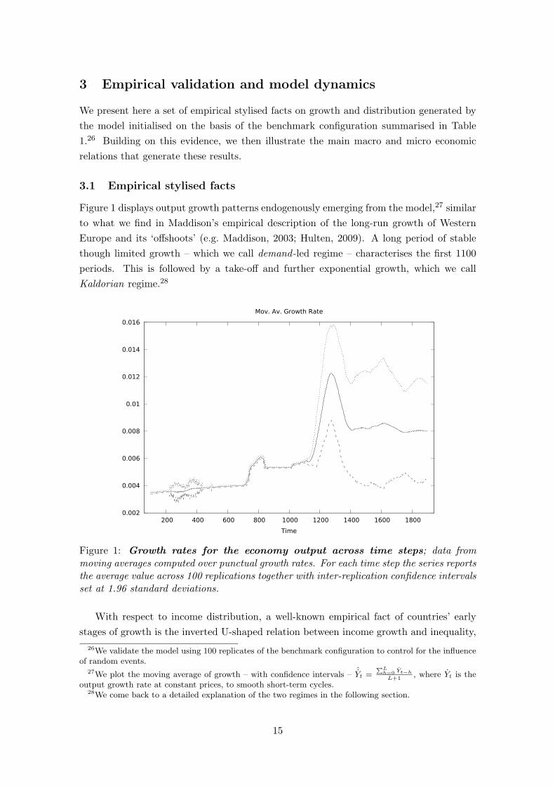
Figure 1 displays output growth patterns endogenously emerging from the model,27 similar

to what we find in Maddison’s empirical description of the long-run growth of Western

Europe and its ‘offshoots’ (e.g. Maddison, 2003; Hulten, 2009). A long period of stable

though limited growth – which we call demand -led regime – characterises the first 1100

periods. This is followed by a take-off and further exponential growth, which we call

Kaldorian regime.28

0.002

0.004

0.006

0.008

0.01

0.012

0.014

0.016

200 400 600 800 1000 1200 1400 1600 1800

Time

Mov. Av. Growth Rate

Figure 1: Growth rates for the economy output across time steps; data frommoving averages computed over punctual growth rates. For each time step the series reportsthe average value across 100 replications together with inter-replication confidence intervalsset at 1.96 standard deviations.

With respect to income distribution, a well-known empirical fact of countries’ early

stages of growth is the inverted U-shaped relation between income growth and inequality,

26We validate the model using 100 replicates of the benchmark configuration to control for the influenceof random events.

27We plot the moving average of growth – with confidence intervals – ˆYt =∑L

h=0Yt−h

L+1, where Yt is the

output growth rate at constant prices, to smooth short-term cycles.28We come back to a detailed explanation of the two regimes in the following section.

15

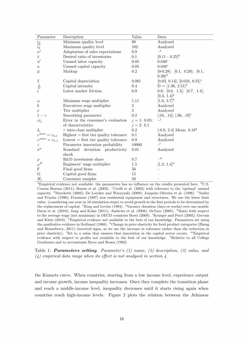
Parameter Description Value Datai2 Minimum quality level 98 Analysedi2 Maximum quality level 102 Analysedas Adaptation of sales expectations 0.9 –a

s Desired ratio of inventories 0.1 [0.11 - 0.25]b

ul Unused labor capacity 0.05 0.046c

u Unused capital capacity 0.05 0.046c

µ Markup 0.2 [0-0.28]; [0.1, 0.28]; [0.1,0.39]d

δ Capital depreciation 0.001 [0.03, 0.14]; [0.016, 0.31]e1

DCapital intensity 0.4 D = [1.36, 2.51]f

ǫ Labor market friction 0.9 0.6; [0.6, 1.5]; [0.7, 1.4];[0.3, 1.4]g

ω Minimum wage multiplier 1.11 [1.6, 3.7]h

b Executives wage multiplier 2 Analysedν Tier multiplier 5 Analysed1− γ Smoothing parameter 0.2 [.04, .14]; [.06, .19]i

ςij Error in the consumer’s evaluationof characteristics

j = 1: 0.05;j = 2: 0.1

–j

δς τ inter-class multiplier 0.2 [-0.8, 2.4] Mean: 0.18k

υmin = υ2,1 Highest = first tier quality tolerance 0.1 Analysedυmax = υ1,1 Lowest = first tier quality tolerance 0.9 Analysedz Parameter innovation probability 10000 –l

σa Standard deviation productivityshock

0.01 Analysed

ρ R&D investment share 0.7 –m

ωE Engineers’ wage multiplier 1.5 [1.2, 1.4]n

F Final good firms 50 –G Capital good firms 15 –Hz Consumer samples 50 –aEmpirical evidence not available: the parameters has no influence on the results presented here. bU.S.Census Bureau (2011); Bassin et al. (2003). cCoelli et al. (2002) with reference to the ‘optimal’ unusedcapacity. dMarchetti (2002); De Loecker and Warzynski (2009); Joaquim Oliveira et al. (1996). eNadiriand Prucha (1996); Fraumeni (1997) non residential equipment and structures. We use the lower limitvalue, (considering one year as 10 simulation steps) to avoid growth in the first periods to be determined bythe replacement of capital. fKing and Levine (1994). gVacancy duration (days or weeks) over one month:Davis et al. (2010); Jung and Kuhn (2011); Andrews et al. (2008); DeVaro (2005). hRatio with respectto the average wage (not minimum) in OECD countries Boeri (2009). iKrueger and Perri (2005); Gervaisand Klein (2010). hEmpirical evidence not available to the best of our knowledge. Parameters set usingthe qualitative evidence in Zeithaml (1988). kChange in price elasticity for food product categories (Zhengand Henneberry, 2011) (inverted signs, as we use the increase in tolerance rather than the reduction inprice elasticity). lSet to a value that ensures that innovation in the capital sector occurs. mEmpiricalevidence with respect to profits not available to the best of our knowledge. oRelative to all CollegeGraduates and to accountants Ryoo and Rosen (1992)

Table 1: Parameters setting. Parameter’s (1) name, (2) description, (3) value, and(4) empirical data range when its effect is not analysed in section 4

the Kuznets curve. When countries, starting from a low income level, experience output

and income growth, income inequality increases. Once they complete the transition phase

and reach a middle-income level, inequality decreases until it starts rising again when

countries reach high-income levels. Figure 2 plots the relation between the Atkinson

16

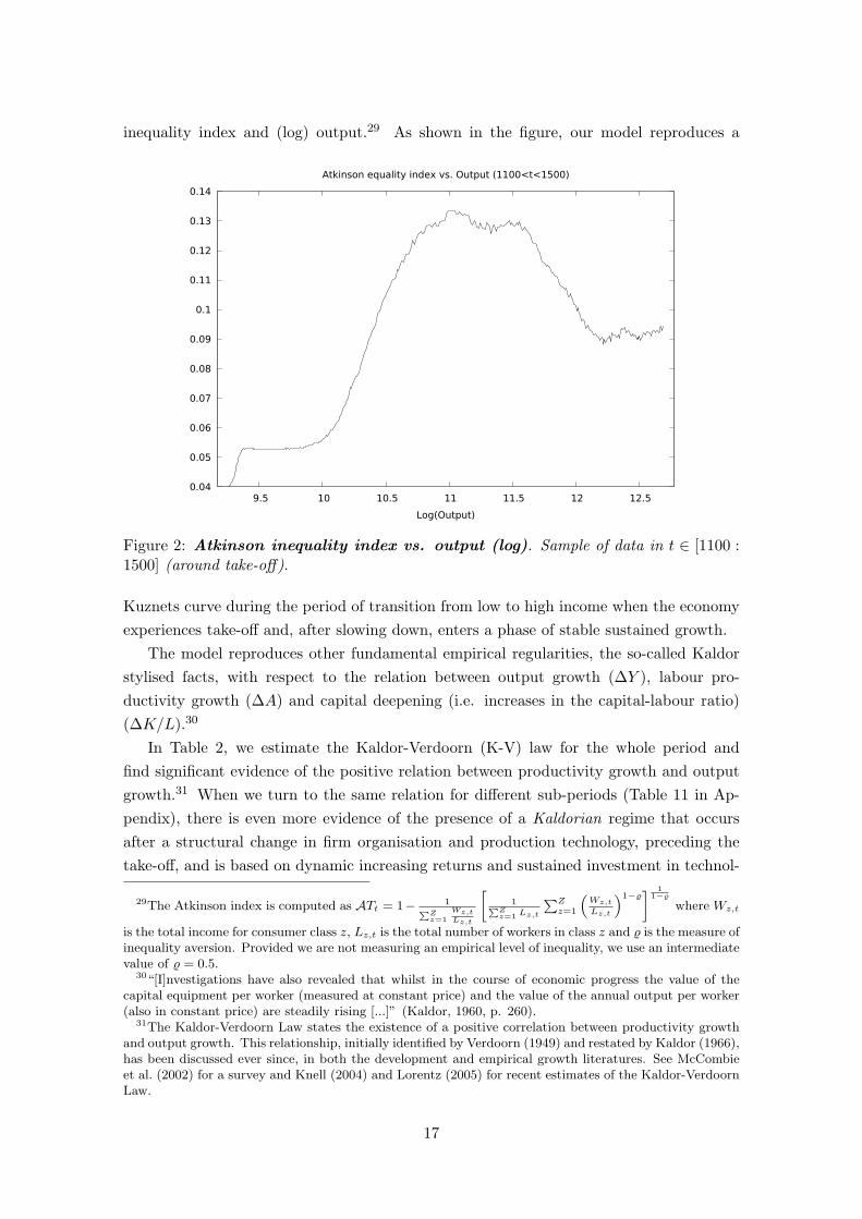
inequality index and (log) output.29 As shown in the figure, our model reproduces a

0.04

0.05

0.06

0.07

0.08

0.09

0.1

0.11

0.12

0.13

0.14

9.5 10 10.5 11 11.5 12 12.5

Log(Output)

Atkinson equality index vs. Output (1100<t<1500)

Figure 2: Atkinson inequality index vs. output (log). Sample of data in t ∈ [1100 :1500] (around take-off).

Kuznets curve during the period of transition from low to high income when the economy

experiences take-off and, after slowing down, enters a phase of stable sustained growth.

The model reproduces other fundamental empirical regularities, the so-called Kaldor

stylised facts, with respect to the relation between output growth (∆Y ), labour pro-

ductivity growth (∆A) and capital deepening (i.e. increases in the capital-labour ratio)

(∆K/L).30

In Table 2, we estimate the Kaldor-Verdoorn (K-V) law for the whole period and

find significant evidence of the positive relation between productivity growth and output

growth.31 When we turn to the same relation for different sub-periods (Table 11 in Ap-

pendix), there is even more evidence of the presence of a Kaldorian regime that occurs

after a structural change in firm organisation and production technology, preceding the

take-off, and is based on dynamic increasing returns and sustained investment in technol-

29The Atkinson index is computed as ATt = 1− 1∑

Zz=1

Wz,tLz,t

[

1∑Zz=1

Lz,t

∑Z

z=1

(

Wz,t

Lz,t

)1−] 1

1−

where Wz,t

is the total income for consumer class z, Lz,t is the total number of workers in class z and is the measure ofinequality aversion. Provided we are not measuring an empirical level of inequality, we use an intermediatevalue of = 0.5.

30“[I]nvestigations have also revealed that whilst in the course of economic progress the value of thecapital equipment per worker (measured at constant price) and the value of the annual output per worker(also in constant price) are steadily rising [...]” (Kaldor, 1960, p. 260).

31The Kaldor-Verdoorn Law states the existence of a positive correlation between productivity growthand output growth. This relationship, initially identified by Verdoorn (1949) and restated by Kaldor (1966),has been discussed ever since, in both the development and empirical growth literatures. See McCombieet al. (2002) for a survey and Knell (2004) and Lorentz (2005) for recent estimates of the Kaldor-VerdoornLaw.

17

ogy. In the early stages of (stagnating) growth, the low pace of change in organisation

and technology does not increase the production capacity to a level sufficient to generate

sustained productivity gains. We show below how this empirical fact in our model depends

on endogenous technical change generating self-reinforcing growth dynamics.32

∆Y (2000)/Y (1) R2 R2corr Obs.

(OLS) ∆A(2000)/A(1) 0.117*** 0.44 0.434 100(0.013)

(LAD) ∆A(2000)/A(1) 0.125*** 100(0.030)

Standard errors (computed with 500 bootstraps) in parentheses; *** p<0.01, ** p<0.05, * p<0.1

Table 2: Kaldor-Verdoorn Law Overall Estimations

Finally, the model reproduces the empirical evidence on capital deepening, i.e. a

constantly increasing ratio of capital per worker for a growing output. In Table 3, we

show LAD estimates of the effect of an increase in the capital labour ratio (∆K/L) on

the output growth rate of output for the whole period. Capital deepening in our model is

∆Y (2000)/Y (1) Const. PseudoR2 Obs.∆K/L(2000)

K/L(1) 10.67*** 2.981*** 0.299 100

(0.505) (0.529)

Standard errors (computed with 400 bootstraps) in parentheses;*** p<0.01, ** p<0.05, * p<0.1

Table 3: Capital deepening and growth. LAD estimates of the growth of K/L ratioover the 2000 periods.

also the mechanism through which output growth affects labour productivity and explains

the Kaldor-Verdoorn Law. Indeed, growth is accelerated by increases in productivity,

which are the result of investment in new capital goods with higher embodied labour

productivity, leading to an increase of the K/L ratio.

3.2 Model dynamics

In the following, we illustrate in more detail the model dynamics that reproduce the

empirical facts discussed above and will enable us to isolate the parameters representing

the core of our analysis. We test the causal structure underlying the growth rate of macro

economic variables using a Vector Autoregressive (VAR) analysis on the fundamentals of

our model. Growth relations are estimated using LAD for three lags, where the sample is

again the 2000 period series of the benchmark configuration, averaged over 100 replicates.

In order to reduce the effect of short term cyclical behaviour we analyse ten periods growth.

32For a more detailed discussion of the cumulative causation nature of the post-take-off period generatedby our model, see Ciarli et al. (2010).

18

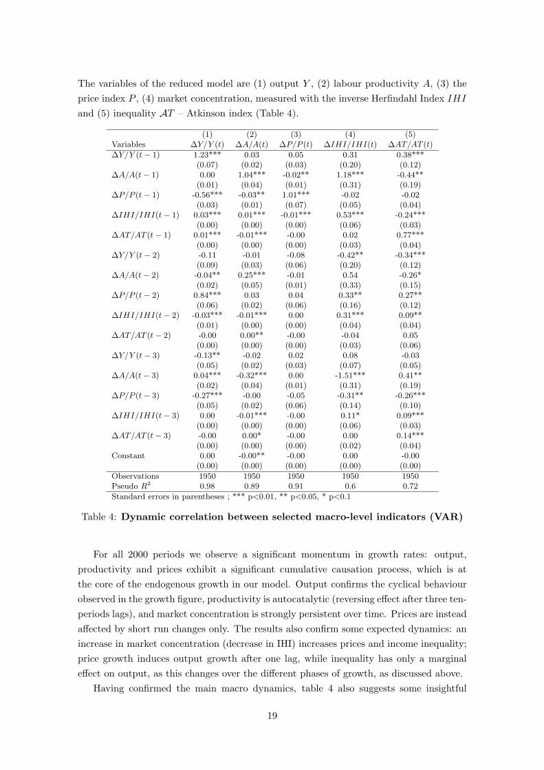
The variables of the reduced model are (1) output Y , (2) labour productivity A, (3) the

price index P , (4) market concentration, measured with the inverse Herfindahl Index IHI

and (5) inequality AT – Atkinson index (Table 4).

(1) (2) (3) (4) (5)Variables ∆Y/Y (t) ∆A/A(t) ∆P/P (t) ∆IHI/IHI(t) ∆AT/AT (t)

∆Y/Y (t− 1) 1.23*** 0.03 0.05 0.31 0.38***(0.07) (0.02) (0.03) (0.20) (0.12)

∆A/A(t− 1) 0.00 1.04*** -0.02** 1.18*** -0.44**(0.01) (0.04) (0.01) (0.31) (0.19)

∆P/P (t− 1) -0.56*** -0.03** 1.01*** -0.02 -0.02(0.03) (0.01) (0.07) (0.05) (0.04)

∆IHI/IHI(t− 1) 0.03*** 0.01*** -0.01*** 0.53*** -0.24***(0.00) (0.00) (0.00) (0.06) (0.03)

∆AT/AT (t− 1) 0.01*** -0.01*** -0.00 0.02 0.77***(0.00) (0.00) (0.00) (0.03) (0.04)

∆Y/Y (t− 2) -0.11 -0.01 -0.08 -0.42** -0.34***(0.09) (0.03) (0.06) (0.20) (0.12)

∆A/A(t− 2) -0.04** 0.25*** -0.01 0.54 -0.26*(0.02) (0.05) (0.01) (0.33) (0.15)

∆P/P (t− 2) 0.84*** 0.03 0.04 0.33** 0.27**(0.06) (0.02) (0.06) (0.16) (0.12)

∆IHI/IHI(t− 2) -0.03*** -0.01*** 0.00 0.31*** 0.09**(0.01) (0.00) (0.00) (0.04) (0.04)

∆AT/AT (t− 2) -0.00 0.00** -0.00 -0.04 0.05(0.00) (0.00) (0.00) (0.03) (0.06)

∆Y/Y (t− 3) -0.13** -0.02 0.02 0.08 -0.03(0.05) (0.02) (0.03) (0.07) (0.05)

∆A/A(t− 3) 0.04*** -0.32*** 0.00 -1.51*** 0.41**(0.02) (0.04) (0.01) (0.31) (0.19)

∆P/P (t− 3) -0.27*** -0.00 -0.05 -0.31** -0.26***(0.05) (0.02) (0.06) (0.14) (0.10)

∆IHI/IHI(t− 3) 0.00 -0.01*** -0.00 0.11* 0.09***(0.00) (0.00) (0.00) (0.06) (0.03)

∆AT/AT (t− 3) -0.00 0.00* -0.00 0.00 0.14***(0.00) (0.00) (0.00) (0.02) (0.04)

Constant 0.00 -0.00** -0.00 0.00 -0.00(0.00) (0.00) (0.00) (0.00) (0.00)

Observations 1950 1950 1950 1950 1950Pseudo R2 0.98 0.89 0.91 0.6 0.72

Standard errors in parentheses ; *** p<0.01, ** p<0.05, * p<0.1

Table 4: Dynamic correlation between selected macro-level indicators (VAR)

For all 2000 periods we observe a significant momentum in growth rates: output,

productivity and prices exhibit a significant cumulative causation process, which is at

the core of the endogenous growth in our model. Output confirms the cyclical behaviour

observed in the growth figure, productivity is autocatalytic (reversing effect after three ten-

periods lags), and market concentration is strongly persistent over time. Prices are instead

affected by short run changes only. The results also confirm some expected dynamics: an

increase in market concentration (decrease in IHI) increases prices and income inequality;

price growth induces output growth after one lag, while inequality has only a marginal

effect on output, as this changes over the different phases of growth, as discussed above.

Having confirmed the main macro dynamics, table 4 also suggests some insightful

19

results on the micro-macro relations in our model. First, while the Kaldor-Verdoorn Law

holds in the long and medium run (Tables 2 and 11 in the Appendix for sub-periods) and

particularly for the post-take-off period, in the short run and accounting for the overall

period, output growth has no significant effect on productivity growth. However, we

observe a direct positive significant effect, albeit small and with three lags, of productivity

growth on output growth. This lagged relation from productivity to output is relatively

straightforward to explain in our model: an increase in output occurs only after removing

factor constraints. Therefore firms first invest in new capital, which may bring an increase

in productivity, and then accommodate demand with an output increase.

The VAR results shed light also on the microeconomic causal relations which are at

the core of our analysis. In particular, we observe that three variables dominate the causal

relations, and affect different aspects of the model dynamics: aggregate productivity (A),

market concentration (IHI) and inequality (AT).

First, aggregate productivity growth first reduces concentration of production and

income and then - 2 lags after - induces a concentration in both variables. On the one

hand an increase in productivity stems from one or more firms investing in new capital

vintages with higher embedded productivity (Eq. in 2.2.3). Investing firms grow in size

(Eq. 2.2.1), which may require to hire a new tier of workers (Eq. in 2.2.2). Indeed, capital

investment increases output and size of capital firms as well (Eq. in 2.3.1). In both

cases, demand increases more than proportionally, due to the emergence of new classes of

workers/consumers, and to the higher wages of the new class of executives (Eq. in 2.2.4

and 2.3.3). The changes in firm size and compensation thus explain the lagged increase

in inequality. On the other hand an increased productivity reduces the cost (price) of the

investing firms (for a given size), attracting more demand from the first consumer classes

(the most populated) and increasing market concentration.

The second causal link then goes from market concentration to income inequality

with one lag: the large increase in demand for a few selected firms requires new tiers of

managers, which by assumption earn more than the existing workers, and receive more

bonuses from firm profits (Eq. 11, 15). The increased demand due to market concentration

than lead to further investment and increase in productivity, as already shown in Table 4.

Third, inequality has a modest effect on productivity: at first it causes productivity

to decrease, following the reduced investment in new machinery, whereas the increased

consumer heterogeneity that accompanies a raise in inequality has a modest positive effect

on productivity.

The VAR results contribute to explaining how micro heterogeneity is responsible for

the two growth regimes – the demand -led and the Kaldorian regimes – identified above.

The initial phase of demand -led growth originates from an initial investment of firms

increasing the number of workers (population), demand for final consumption, income,

firm size and further demand for labour. During this first period, investment occurs at

the rate of capital depreciation and population growth. The second stage of exponential

growth is related to market concentration and a sudden increase in capital investment

20

by the few firms that start leading the market. The large capital investment of these

firms induces large jumps in aggregate productivity, which sets off a cumulative causation

process of the Kaldorian type (Kaldor, 1966): price reduction, increased profits, increase

in final demand, sustained investment in R&D and new capital vintages, with increasing

productivity embedded in the capital that sustains the exponential pattern.

In the following section we analyse how the the initial conditions that define the struc-

ture of an economy and the way in which this unfolds through time affect output growth

and income inequality. The effect of productivity (A) is captured by the parameter that

defines the speed at which capital good firms increase the productivity embodied in new

capital goods, σα (Eq. 23). The effect of market concentration is captured by the parame-

ter that defines the organisation of production, i.e., the pace at which new tiers of workers

and managers are created for a given increase in production capacity, increasing firm size

and final demand, ν (Eqs. 5 and 19). We then distinguish between direct and indirect

effect of inequality. The first one, observed in the linear relations analysed in the VAR,

is captured by the wage multiplier, b (Eqs. 11 and 26). The second effect is due to the

changes in consumption patterns following the emergence of new classes of consumers and

is captured by both the across-class differences in consumer preferences, υmin and υmax,

and the initial variety in the characteristics of the products they select, i2,f and i1,f (t).

4 Simulation results: structural differences in technology,

organisation and demand

We now turn to the analysis of the effect of exogenous structural conditions on output

growth and income distribution. In particular, we focus on the effect of the following

combinations of parameters defining the different aspects of the structure of an economy:

Composition of production and demand: variance of the distribution of a product’s

quality and price (standard deviation (sd) of i2,f ) and variance in the preferences of dif-

ferent earning classes (|υmax − υmin|) (Section 4.1). The relation between the speed of

technological change in capital vintages (σa) and in the firm organisational structure

(number of tiers for a given number of shop floor workers, ν) (Section 4.2).

The relation between the firm organisational structure (ν) and the distribution of wages

and premia (b) (Section 4.3).

For each combination of the parameters we ran 20 replicates with different random

seeds for 2000 time periods and report the average over the replicates. In Appendix A,

we show that 20 replicates are sufficient to wipe out the effect of random initialisations.

We then estimated if the result of each combination of parameters is significantly different

form the benchmark case with a bootstrapped quantile regression of the type lnY =

α+βijD1iD2j + ǫ, where the D1iD2j are all the possible two way interactions of the pair

of analysed parameters, except for the benchmark which is the reference value.

21

4.1 Composition of production and demand

It is a well-established empirical finding that income growth is accompanied by changes

in the composition of production in terms of sectoral specialisation and product variety

through quality differentiation (e.g. Sirquin, 1988; Maddison, 2001; Dosi et al., 1994a;

Prebish, 1950; Hidalgo and Hausmann, 2009; Saviotti, 1996). Accordingly, product differ-

entiation is accompanied by a change in consumer preferences and consumption patterns

(Maddison, 2001), which become more heterogeneous across consumers as a result of the

increased variety of production and income classes.

Here we analyse the joint effect of the initial good’s quality differentiation across firms

and of the emerging different distributions of preferences across consumer classes. With

reference to the model, we vary the value of the standard deviation of product quality

distribution across firms(

s.d. i2 ∼ U [i2, i2])

– assuming that a relatively higher quality

is related to a proportionally higher markup33 – and the difference in the tolerance level

across consumer classes(

υmax − υmin)

.34

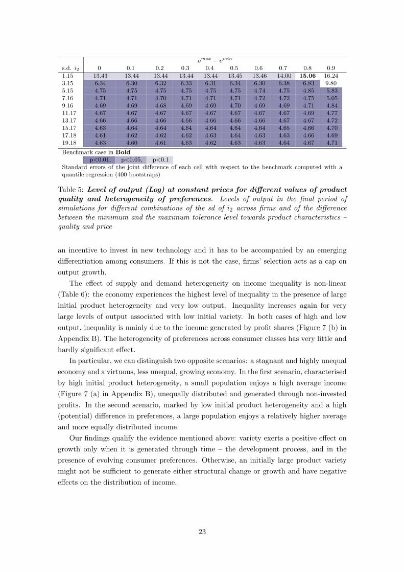
Table 5 shows the level of output (log) for different combinations of sd i2 and υmax −

υmin and whether the difference is statistically significant with respect to the benchmark

case (low product variety and high consumer heterogeneity).35 Our findings only partially

support the proposition that a higher initial variety (across both goods and consumers)

is linked to faster output growth. The table shows two main results: (i) a high initial

variety in the quality of goods induces a low growth when goods are substitutes, as in our

model; (ii) the heterogeneity between consumer preferences increases output growth only

when it is very large and its effect is not dwarfed by the counter-effect of an initially large

product variety.

These results are explained by the fact that too large a variety of products during the

initial time periods does not spark the take-off. In the initial periods, aggregate demand

is, in fact, too low to be an incentive for firms to invest in new capital. Therefore, firm

selection induced by high variety has the only effect of reducing the number of overall

vacancies, keeping demand low. With no demand effect, the cumulative process never gets

started, and although the economy experiences an endogenous growth, this is the lower,

the higher the initial market concentration. This result is confirmed by the low aggregated

labour productivity observed for a very low number of workers, in the presence of high

product heterogeneity.36

In other words, in order to induce the take off, product variety should develop over

time, once the economy has already undergone a growth in demand such that firms have

33Several industry studies support this hypothesis, e.g. Deltas et al. (2011), Corrocher and Guerzoni(2009) and Verboven (1999).

34We use the distance between the minimum and the maximum tolerance level because the standarddeviation is endogenous to the model and depends on the growth pattern (and the generation of incomeclasses). The distance allows to compare the parameters’ space for high and low growth on a fixed set ofpossible outcomes.

35The significance of each combination was estimated with a bootstrapped quantile regression. Resultsof the regression are available from the authors.

36Figures are available from the authors.

22

υmax− υmin

s.d. i2 0 0.1 0.2 0.3 0.4 0.5 0.6 0.7 0.8 0.9

1.15 13.43 13.44 13.44 13.44 13.44 13.45 13.46 14.00 15.06 16.243.15 6.34 6.30 6.32 6.33 6.31 6.34 6.30 6.38 6.83 9.805.15 4.75 4.75 4.75 4.75 4.75 4.75 4.74 4.75 4.85 5.837.16 4.71 4.71 4.70 4.71 4.71 4.71 4.72 4.72 4.75 5.059.16 4.69 4.69 4.68 4.69 4.69 4.70 4.69 4.69 4.71 4.8411.17 4.67 4.67 4.67 4.67 4.67 4.67 4.67 4.67 4.69 4.7713.17 4.66 4.66 4.66 4.66 4.66 4.66 4.66 4.67 4.67 4.7215.17 4.63 4.64 4.64 4.64 4.64 4.64 4.64 4.65 4.66 4.7017.18 4.61 4.62 4.62 4.62 4.63 4.64 4.63 4.63 4.66 4.6919.18 4.63 4.60 4.61 4.63 4.62 4.63 4.63 4.64 4.67 4.71

Benchmark case in Bold

p<0.01, p<0.05, p<0.1Standard errors of the joint difference of each cell with respect to the benchmark computed with aquantile regression (400 bootstraps)

Table 5: Level of output (Log) at constant prices for different values of productquality and heterogeneity of preferences. Levels of output in the final period ofsimulations for different combinations of the sd of i2 across firms and of the differencebetween the minimum and the maximum tolerance level towards product characteristics –quality and price

an incentive to invest in new technology and it has to be accompanied by an emerging

differentiation among consumers. If this is not the case, firms’ selection acts as a cap on

output growth.

The effect of supply and demand heterogeneity on income inequality is non-linear

(Table 6): the economy experiences the highest level of inequality in the presence of large

initial product heterogeneity and very low output. Inequality increases again for very

large levels of output associated with low initial variety. In both cases of high and low

output, inequality is mainly due to the income generated by profit shares (Figure 7 (b) in

Appendix B). The heterogeneity of preferences across consumer classes has very little and

hardly significant effect.

In particular, we can distinguish two opposite scenarios: a stagnant and highly unequal

economy and a virtuous, less unequal, growing economy. In the first scenario, characterised

by high initial product heterogeneity, a small population enjoys a high average income

(Figure 7 (a) in Appendix B), unequally distributed and generated through non-invested

profits. In the second scenario, marked by low initial product heterogeneity and a high

(potential) difference in preferences, a large population enjoys a relatively higher average

and more equally distributed income.

Our findings qualify the evidence mentioned above: variety exerts a positive effect on

growth only when it is generated through time – the development process, and in the

presence of evolving consumer preferences. Otherwise, an initially large product variety

might not be sufficient to generate either structural change or growth and have negative

effects on the distribution of income.

23

υmax− υmin

s.d. i2 0 0.1 0.2 0.3 0.4 0.5 0.6 0.7 0.8 0.9

1.15 0.06 0.06 0.06 0.06 0.06 0.06 0.06 0.07 0.08 0.093.15 0.02 0.02 0.02 0.02 0.02 0.02 0.02 0.02 0.02 0.055.15 0.03 0.03 0.03 0.03 0.03 0.03 0.03 0.03 0.03 0.027.16 0.04 0.04 0.04 0.04 0.04 0.04 0.04 0.04 0.04 0.039.16 0.05 0.05 0.05 0.05 0.05 0.05 0.05 0.05 0.04 0.0411.17 0.06 0.06 0.06 0.06 0.06 0.06 0.06 0.06 0.05 0.0513.17 0.07 0.07 0.07 0.07 0.07 0.07 0.07 0.06 0.06 0.0615.17 0.08 0.08 0.08 0.08 0.08 0.07 0.07 0.07 0.06 0.0617.18 0.09 0.09 0.09 0.09 0.08 0.08 0.08 0.07 0.07 0.0619.18 0.10 0.10 0.10 0.10 0.09 0.08 0.08 0.08 0.07 0.07

Benchmark case in Bold

p<0.01, p<0.05, p<0.1Standard errors of the joint difference of each cell with respect to the benchmark computed witha quantile regression (400 bootstraps)

Table 6: Atkinson index for different values of product quality and heterogeneityof preferences. Levels of output in the final period of simulations for different combi-nations of the sd of i2 across firms and of the difference between the minimum and themaximum tolerance level towards product characteristics – quality and price

4.2 Organisation and production technology

We then analyse the joint effect of production technology (σa) and organisational structure

(ν). Production technology refers to the capital structure of firms, while the organisational

structure reflects the hierarchical structure of labour.

At the firm level, a higher number of layers (low ν), ceteris paribus, increases the

number of workers and the production costs while a wider distribution of the R&D outcome

(high σa) reduces the number of workers.At the industry level, larger potential productivity

gains should result in the most efficient firm growing and dominating the market However,

the cost associated with an increase in the number of management layers imposes a trade-

off between capital investment and growth. Finally, at the macro level both parameters

should positively affect growth via effective demand. The two parameters are expected

to increase inequality as well: (i) a higher number of tiers generate a higher dispersion in

income distribution by construction; and (ii) higher productivity allows for higher profits

to benefit the higher tiers of workers.

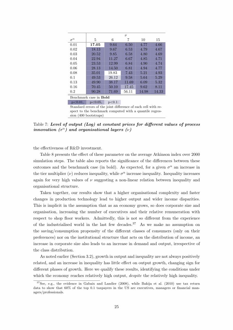
Table 7 confirms the expectations on economic growth. It shows the Log of output

levels at constant prices after 2000 simulation steps for various values of the parameters

defining organisational structure and production technology. The table also shows whether

output is significantly different from the benchmark case for each value’s combination. An

increase in σa positively and significantly affects output, while an increase in ν – reducing

the number of layers, ceteris paribus – negatively affects output. The results clearly

demonstrate that small reductions in organisational complexity require large changes in

production technology to achieve the same level of output growth. Finally, the reduced

significance of the difference with respect to the benchmark is due to the increased volatility

in the outcome of R&D investments: large values of σa increase the variance of output

across replicates, showing that a higher output for large σa is conditional on increasing

24

νσα 5 6 7 10 150.01 17.05 9.64 6.50 4.77 4.660.02 18.13 9.67 6.53 4.79 4.670.03 20.52 9.85 6.58 4.80 4.690.04 22.94 11.27 6.67 4.85 4.710.05 23.53 12.99 6.84 4.90 4.740.06 28.13 14.50 6.81 4.94 4.770.08 35.01 19.83 7.43 5.21 4.930.1 49.53 26.12 9.58 5.64 5.290.13 49.90 38.17 11.69 6.09 5.320.16 70.45 50.10 17.45 9.62 8.110.2 90.28 71.69 56.11 14.98 14.33

Benchmark case in Bold

p<0.01, p<0.05, p<0.1:

Standard errors of the joint difference of each cell with re-spect to the benchmark computed with a quantile regres-sion (400 bootstraps)

Table 7: Level of output (Log) at constant prices for different values of processinnovation (σα) and organisational layers (ν)

the effectiveness of R&D investment.

Table 8 presents the effect of these parameter on the average Atkinson index over 2000

simulation steps. The table also reports the significance of the differences between these

outcomes and the benchmark case (in bold). As expected, for a given σα an increase in

the tier multiplier (ν) reduces inequality, while σα increase inequality. Inequality increases

again for very high values of ν suggesting a non-linear relation between inequality and

organisational structure.

Taken together, our results show that a higher organisational complexity and faster

changes in production technology lead to higher output and wider income disparities.

This is implicit in the assumption that as an economy grows, so does corporate size and

organisation, increasing the number of executives and their relative remuneration with

respect to shop floor workers. Admittedly, this is not so different from the experience

of the industrialised world in the last few decades.37 As we make no assumption on

the saving/consumption propensity of the different classes of consumers (only on their

preferences) nor on the institutional structure that acts on the distribution of income, an

increase in corporate size also leads to an increase in demand and output, irrespective of

the class distribution.

As noted earlier (Section 3.2), growth in output and inequality are not always positively

related, and an increase in inequality has little effect on output growth, changing sign for

different phases of growth. Here we qualify these results, identifying the conditions under

which the economy reaches relatively high output, despite the relatively high inequality.

37See, e.g., the evidence in Gabaix and Landier (2008), while Bakija et al. (2010) use tax returndata to show that 60% of the top 0.1 taxpayers in the US are executives, managers or financial man-agers/professionals.

25

νσα 5 6 7 10 150.01 0.058 0.022 0.017 0.017 0.0230.02 0.064 0.022 0.017 0.017 0.0230.03 0.079 0.022 0.017 0.017 0.0230.04 0.092 0.028 0.017 0.017 0.0220.05 0.095 0.035 0.017 0.018 0.0220.06 0.113 0.042 0.017 0.018 0.0220.08 0.142 0.067 0.018 0.018 0.0230.1 0.182 0.092 0.027 0.019 0.0240.13 0.173 0.134 0.035 0.021 0.0240.16 0.192 0.156 0.061 0.034 0.0360.2 0.195 0.175 0.138 0.058 0.069

Benchmark case in Bold

p<0.01, p<0.05, p<0.1:

Standard errors of the joint difference of each cell withrespect to the benchmark computed with a quantileregression (400 bootstraps)

Table 8: Atkinson index for different values of process innovation (σα) andorganisational layers ν. Atkinson index averaged across the 2000 simulation steps

4.3 Organization and wage structure

To realise a better understanding of the effect the parameters that directly determine

changes in the income distribution in our model, we focus on the joint effect of the deter-

minants of the organisation (ν) and the wage (b) structure. The two parameters have two

symmetric effects on the supply and the demand side of the economy. On the supply side,

a higher number of layers (lower ν) and/or a higher wage multiplier (higher b) directly

increase the firm’s cost. This may also result in a higher dispersion of prices across firms

over time. On the demand side, a reduction in ν and an increase in b increases aggregate

income and income disparities, and increase the heterogeneity in demand preferences and

the range of affordable products.

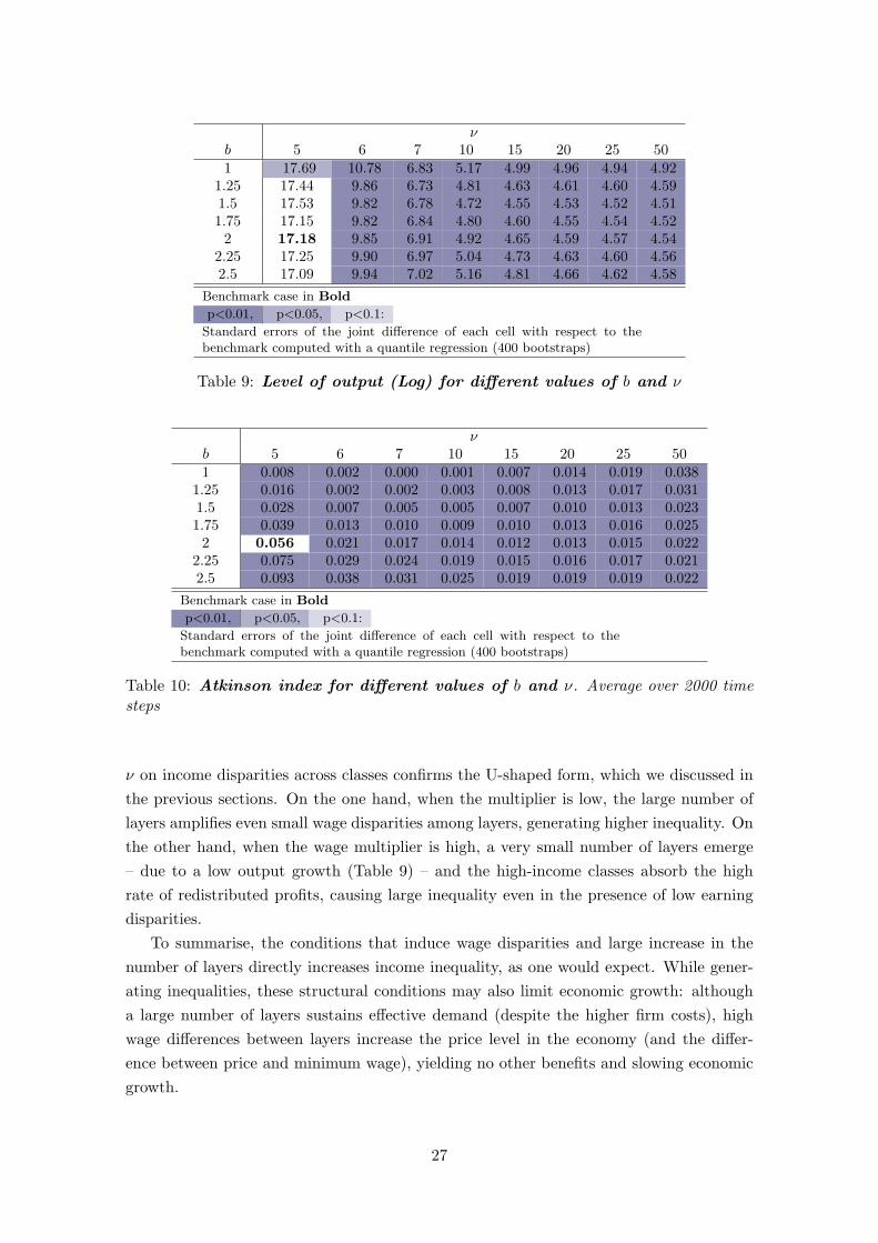
Table 9 shows the effect of the organisational complexity and wage dispersion on the

log of output at constant price after 2000 simulation steps. It also reports the significance

of the differences between the outcomes under each parameter combination and that of

the benchmark (in bold). On the one hand, the higher the organisational complexity, the

higher is the output growth: the increase in the number of consumers directly translates

into higher effective demand with a direct positive effect on growth. On the other hand,

the higher the wage multiplier, the lower is the output growth: assuming no direct effect

of wages on productivity, the increase in cost generated by high disparities in wages slows

down long-run growth. However, this second effect is not significant overall.

In Table 10, we observe the impact of the organisational and payment structure on in-

equality (Atkinson index averaged over 2000 simulation steps) and their significance with

respect to the benchmark case (in bold). As expected, increasing the wage multiplier me-

chanically raises the income disparities across households. The effect of the tier multiplier

26

νb 5 6 7 10 15 20 25 501 17.69 10.78 6.83 5.17 4.99 4.96 4.94 4.92

1.25 17.44 9.86 6.73 4.81 4.63 4.61 4.60 4.591.5 17.53 9.82 6.78 4.72 4.55 4.53 4.52 4.511.75 17.15 9.82 6.84 4.80 4.60 4.55 4.54 4.522 17.18 9.85 6.91 4.92 4.65 4.59 4.57 4.54

2.25 17.25 9.90 6.97 5.04 4.73 4.63 4.60 4.562.5 17.09 9.94 7.02 5.16 4.81 4.66 4.62 4.58

Benchmark case in Bold

p<0.01, p<0.05, p<0.1:

Standard errors of the joint difference of each cell with respect to thebenchmark computed with a quantile regression (400 bootstraps)

Table 9: Level of output (Log) for different values of b and ν

νb 5 6 7 10 15 20 25 501 0.008 0.002 0.000 0.001 0.007 0.014 0.019 0.038

1.25 0.016 0.002 0.002 0.003 0.008 0.013 0.017 0.0311.5 0.028 0.007 0.005 0.005 0.007 0.010 0.013 0.0231.75 0.039 0.013 0.010 0.009 0.010 0.013 0.016 0.0252 0.056 0.021 0.017 0.014 0.012 0.013 0.015 0.022

2.25 0.075 0.029 0.024 0.019 0.015 0.016 0.017 0.0212.5 0.093 0.038 0.031 0.025 0.019 0.019 0.019 0.022

Benchmark case in Bold

p<0.01, p<0.05, p<0.1:

Standard errors of the joint difference of each cell with respect to thebenchmark computed with a quantile regression (400 bootstraps)

Table 10: Atkinson index for different values of b and ν. Average over 2000 timesteps

ν on income disparities across classes confirms the U-shaped form, which we discussed in

the previous sections. On the one hand, when the multiplier is low, the large number of

layers amplifies even small wage disparities among layers, generating higher inequality. On

the other hand, when the wage multiplier is high, a very small number of layers emerge

– due to a low output growth (Table 9) – and the high-income classes absorb the high

rate of redistributed profits, causing large inequality even in the presence of low earning

disparities.

To summarise, the conditions that induce wage disparities and large increase in the

number of layers directly increases income inequality, as one would expect. While gener-

ating inequalities, these structural conditions may also limit economic growth: although

a large number of layers sustains effective demand (despite the higher firm costs), high

wage differences between layers increase the price level in the economy (and the differ-

ence between price and minimum wage), yielding no other benefits and slowing economic

growth.

27

5 Concluding remarks

A large and diverse literature has pointed to solid empirical evidence suggesting mutual

effects on the relations between structural changes in different aspects of the economy and

economic growth. We argue that the structure of production and the way in which it is

organised by firms, together with the structure of demand, are the main candidates to

explain the growth differences we observe across countries and within countries over time.

We propose a model that accounts for these three different dimensions of structural

change, generating different patterns of growth and income distribution. The relations

between the different aspects of structural change on the supply and the demand side of

the economy occur through the micro behaviour of firms and consumers.

We show that the model is able to replicate a number of stylised facts. We then analyse

the main causal relations between the different aspects of structural change and find that

productivity growth, firm size and market concentration, and the distribution of income

across income classes dominate the causal relations and affect most aspects of the model

dynamics. First, firm selection generates an oligopolistic competition in the final good

sector which is accompanied by a high growth in capital investments by the expanding

firms. Second, it is this concentration of demand and investments that produces high R&D

investments in the capital sector, leading to rapid changes in the production technology,

quickly absorbed by final good firms. Third, firm selection and market concentration result

from the variety in the composition of production in terms of cost and quality differences,

and from the heterogeneity of consumption patterns that emerges across consumer classes.

Fourth, the organisation of production – number of managerial tiers – is what generates

cost differences and price dispersion across firms, and different wage classes. The earning

structure amplifies these differences. Capital investment introduces more heterogeneity in

the model, leading to more selection and market concentration, sustaining this cumulative

causation dynamics.

For given values of the parameters that define the three aspects of the structure of

an economy and the way in which this unfolds through time, these recursive dynamics

generate the take-off and what we called the Kaldorian phase of growth. Indeed, the

concentration of production on a reduced number of firms also affects the distribution of

income.

In the last part of the paper we analyse the conditions under which these parameters

generate the take-off and find the following main results. Product variety plays a relevant

role in the economic growth of an economy only when it is generated through time and

when it is accompanied by a broad heterogeneity in consumer preferences. When product

heterogeneity is broad during the initial stages of stagnant growth, strong firm selection

before the expansion of demand level and variety hinders the cumulative feedbacks dis-

cussed above. The economic quasi-stagnation is also accompanied by a large inequality

due to the low incentive to invest and the consequent high proportion of distributed prof-

its. Stretching the argument a little further in a long-run growth perspective, an economy

28

gains from diversifying once it has built an industrial base sufficient to induce a high in-

ternal demand and investment. An initial big push toward industrial diversification is not

conducive to high growth.

Organisational structures that lead to a large number of organisational tiers, as well as

large productivity gains embodied in capital goods, lead to higher output levels, despite

generating higher income inequality, which after the take-off has a negative effect on

growth. However, the number of organisational tiers has a non linear effect on inequality,

which increases again for very flat organisations. This is again due to a condition of

stagnating economy where profits are distributed as bonuses and not invested.

Firms’ organisational and earning structures affect economic growth both via the

level of aggregate demand and income disparities. Despite increasing average wages and

prices, complex hierarchical structures sustain aggregate demand in the long run, induc-

ing demand-led cumulative causation growth. However, the increase in earning disparities

and inequality in this case limits growth, due to the high cost of (managerial) labour with

respect to the minimum wage which reduces the purchasing power of the large bulk of the

consumers, lower investments and slow productivity changes.

29

References

Abowd, John M., Francis Kramarz, and David N. Margolis, “High Wage Workers

and High Wage Firms,” Econometrica, 1999, 67 (2), 251–333.

Acemoglu, Daron and James A. Robinson, “Economic Backwardness in Political

Perspective,” American Political Science Review, 2006, 100 (01), 115–131.

and Simon Johnson, “Unbundling Institutions,” Journal of Political Economy, Oc-

tober 2005, 113 (5), 949–995.

Adam, Christopher and Stefan Dercon, “The political economy of development: an

assessment,” Oxford Review of Economic Policy, 2009, 25 (2), 173–189.

Aghion, Philippe and Peter Howitt, Endogenous Growth Theory, Vol. 1 of MIT Press

Books, The MIT Press, December 1998.

, Eve Caroli, and Cecilia Garcıa-Pe nalosa, “Inequality and Economic Growth:

The Perspective of the New Growth Theories,” Journal of Economic Literature, Dec

1999, 37 (4), 1615–1660.

Akerlof, George A. and Robert J. Shiller, Animal spirits: how human psychology

drives the economy, and why it matters for global capitalism, Princeton University Press,

2009.

Andrews, Martyn J., Steve Bradley, David N. Stott, and Richard Upward,

“Successful Employer Search? An Empirical Analysis of Vacancy Duration Using Micro

Data,” Economica, 2008, 75 (299), 455–480.

Aoki, Masanao and Hiroshi Yoshikawa, “Demand saturation–creation and economic

growth,” Journal of Economic Behavior & Organization, 2002, 48, 127–154.

Arifovic, Jasmina, James Bullard, and John Duffy, “The Transition from Stagna-

tion to Growth: An Adaptive Learning Approach,” Journal of Economic Growth, July

1997, 2 (2), 185–209.

Atkinson, Anthony B., “The distribution of earnings in OECD countries,” International

Labour Review, 2007, 146 (1-2), 41–60.

Babutsidze, Zakaria, “How Do Consumers Make Choices? A Summary of Evidence

fromMarketing and Psychology,” Technical Report, INTECH United Nations University

2007.

Bakija, Jon, Adam Cole, and Bradley T. Heim, “Jobs and Income Growth of Top

Earners and the Causes of Changing Income Inequality: Evidence from U.S. Tax Return

Data,” Department of Economics Working Papers 2010-24, Williams College 2010.

30

Barro, Robert, “Economic Growth in a Cross Section of Countries,” Quarterly Journal

of Economics, 1991, 106(2), 407–443.

Bassin, William M., Michael T. Marsh, and Stefanie Walitzer, “A Macroeconomic

Analysis Of Inventory/Sales Ratios,” Journal of Business & Economics Research, 2003,

1 (10), 37–45.

Blanchard, Olivier J., “The Production and Inventory Behavior of the American Au-

tomobile Industry,” Journal of Political Economy, 1983, 91 (3), pp. 365–400.

Blanchflower, David G. and Andrew J. Oswald, “The Wage Curve: An Entry

Written for the New Palgrave, 2nd Edition,” Discussion Paper 2138, IZA, Bonn May

2006.

Blinder, Alan S., “Inventories and Sticky Prices: More on the Microfoundations of

Macroeconomics,” The American Economic Review, 1982, 72 (3), 334–348.

, “Why are prices sticky? Preliminary results from an interview study,” American

Economic Review, 1991, 81 (2), 89–96.

Boeri, Tito, “Setting the Minimum Wage,” IZA Discussion Papers 4335, Institute for

the Study of Labor (IZA) July 2009.

Borsch-Supan, Axel H., “Panel Data Analysis of the Beveridge Curve: Is There a

Macroeconomic Relation between the Rate of Unemployment and the Vacancy Rate?,”

Economica, Aug 1991, 58 (231), 279–297.

Bottazzi, Giulio and Marco Grazzi, “Wage structure in Italian Manufacturing firms,”

LEM Working Paper Series 2007/05, Laboratory of Economics and Management,

Sant’Anna School of Advanced Studies, Pisa February 2007.

Brown, Charles and James Medoff, “The Employer Size–Wage Effect,” Journal of

Political Economy, October 1989, 97 (5), 1027–1059.

Buchanan, Mark, “Economics: Meltdown modelling. Could agent-based computer mod-

els prevent another financial crisis?,” Nature, 2009, 460, 680–682.

Bureau of Labour Statistics, “New Quarterly Data From BLS on Business Employ-

mentDynamics By Size of Firm,” News, United States Department for Labor, Washing-

ton December 2005. Accessed on 06.11.2010.

Caroli, Eve and John Van Reenen, “Skill–Biased Organizational Change? Evidence

from a Panel of British and French Establishments,” Quarterly Journal of Economics,

2001, 116 (4), 1449–1492.

Celsi, Richard L. and Jerry C. Olson, “The Role of Involvement in Attention and

Comprehension Processes,” Journal of Consumer Research, 1988, 15 (2), 210–224.

31

Cesaratto, S., F. Serrano, and A. Stirati, “Technical Change, Effective Demand and

Employment,” Review of Political Economy, 2003, 5(1), 33–52.

Chiarella, Carl, Disequilibrium, growth, and labor market dynamics: macro perspectives,

Springer, 2000.

Chiaromonte, Francesca and Giovanni Dosi, “Heterogeneity, Competition, and

Macroeconomics Dynamics,” Structural Change and Economic Dynamics, 1993, 4(1),

39–63.

Ciarli, Tommaso, Andre Lorentz, Maria Savona, and Marco Valente, “The

Effect of Consumption and Production Structure on Growth and Distribution. A Micro

to Macro Model,” Metroeconomica, 2010, 61 (1), 180–218.

Coelli, Tim, Emili Grifell-Tatje, and Sergio Perelman, “Capacity utilisation and

profitability: A decomposition of short-run profit efficiency,” International Journal of

Production Economics, 2002, 79 (3), 261–278.

Colander, D., P. Howitt, A. Kirman, A. Leijonhufvud, and P. Mehrling, “Be-

yond DSGE models: toward an empirically based macroeconomics,” American Eco-

nomic Review, 2008, 98 (2), 236–240.

Cooper, R.W and J.C. Haltiwanger, “On the Nature of Capital Adjustment Costs,”

Review of Economic Studies, 2006, 73(3), 611–633.

Cornwall, John and Wendy Cornwall, “Growth Theory and Economic Structure,”

Economica, 1994, 61 (242), 237–251.

Corrocher, Nicoletta and Marco Guerzoni, “Product variety and price strategy in

the ski manufacturing industry,” Journal of Evolutionary Economics, August 2009, 19

(4), 471–486.

Criscuolo, Chiara, “Employer Size - Wage Effect: A Critical Review and an Econometric

Analysis,” SSRN eLibrary, 2000.

Cummins, Jason G. and Giovanni L. Violante, “Investment-Specific Technical

Change in the United States (1947-2000): Measurement and Macroeconomic Conse-

quences,” Review of Economic Dynamics, 2002, 5 (2), 243 – 284.

Davis, Steven J., R. Jason Faberman, and John C. Haltiwanger, “The

Establishment-Level Behavior of Vacancies and Hiring,” Working Paper 16265, National

Bureau of Economic Research August 2010.

Dawar, Niraj and Philip Parker, “Marketing Universals: Consumers’ Use of Brand

Name, Price, Physical Appearance, and Retailer Reputation as Signals of Product Qual-

ity,” The Journal of Marketing, 1994, 58 (2), 81–95.

32

Dawid, Herbert and Giorgio Fagiolo, “Agent-based models for economic policy de-

sign: Introduction to the special issue,” Journal of Economic Behavior and Organiza-

tion, 2008, 67 (2), 351–354.

and M. Neugart, “Agent-based Models for Economic Policy Design,” Eastern Eco-

nomic Journal, 2010, 37, 44–50.

and Willy Semmler, “Introduction to the special issue: Computational perspectives

in economics and finance: Methods, dynamic analysis and policy modeling,” Journal of

Economic Dynamics and Control, 2010, 34 (9), 1529 – 1530. ¡ce:title¿Computational

perspectives in economics and finance: Methods,dynamic analysis and policy model-

ing¡/ce:title¿.

Deissenberg, C., S. Van Der Hoog, and H. Dawid, “EURACE: A massively parallel

agent-based model of the European economy,” Applied Mathematics and Computation,

2008, 204 (2), 541–552.

Delli Gatti, Domenico, Edoardo Gaffeo, and Mauro Gallegati, “Complex agent-

based macroeconomics: a manifesto for a new paradigm,” Journal of Economic Inter-

action and Coordination, 2010, 5, 111–135. 10.1007/s11403-010-0064-8.

, Saul Desiderio, Edoardo Gaffeo, Pasquale Cirillo, and Mauro Galle-

gati, Macroeconomics from the Bottom-up, Vol. 1 of New Economic Windows, Milan:

Springer, 2011.

Deltas, George, Thanasis Stengos, and Eleftherios Zacharias, “Product line pric-

ing in a vertically differentiated oligopoly,” Canadian Journal of Economics, 2011, 44

(3), 907–929.

Denison, E. F., “Why growth rates differ,” Technical Report, Brooking Inst. Washington

D.C. 1967.

, “Accounting for slower economic growth,” Technical Report, Brooking Inst. Washing-

ton D.C. 1979.

Desmet, Klaus and Stephen L. Parente, “The evolution of markets and the revolu-

tion of industry: A quantitative model of England’s development, 1300-2000,” Working

Papers 2009-06, Instituto Madrileno de Estudios Avanzados (IMDEA) Ciencias Sociales

May 2009.

DeVaro, Jed, “Employer Recruitment Strategies and the Labor Market Outcomes of

New Hires,” Economic Inquiry, 2005, 43 (2), 263–282.

Doms, M. and T. Dunne, “Capital Adjustment Patterns in Manufacturing Plants,”

Review of Economic Dynamics, 1998, 1, 409–429.

33

Dosi, Giovanni, Chris Freeman, and Silvia Fabiani, “The Process of Economic

Development: Introducing Some Stylized Facts and Theories on Technologies, Firms

and Institutions,” Industrial and Corporate Chance, 1994, 3 (1), 1–45.

, Giorgio Fagiolo, and Andrea Roventini, “Schumpeter Meeting Keynes: A Policy–

Friendly Model of Endogenous Growth and Business Cycles,” Journal of Economic

Dynamics and Control, 2010, 34, 1748–1767.

, Silvia Fabiani, Roberta Aversi, and Mara Meacci, “The Dynamics of Interna-

tional Differentiation: A Multi-Country Evolutionary Model,” Industrial and Corporate

Change, 1994, 3 (1), 225–242.

Durlauf, Steven N. and Danny T. Quah, “The New Empirics of Economic Growth,”

Discussion paper 384, Centre For Economic Performance January 1998. Prepared for

the ‘Handbook of Macroeconomics’, Taylor J. and Woodford M. (eds.).

Economic Commission for Europe, Economic Survey Of Europe, 2004, United Na-

tions, 2004.

Fabiani, Silvia, Martine Druant, Ignacio Hernando, Claudia Kwapil, Bettina

Landau, Claire Loupias, Fernando Martins, Thomas Matha, Roberto Sab-

batini, Harald Stahl, and Ad Stokman, “What firms’ surveys tell us about price-

setting behaviour in the euro area.,” International Journal of Central Banking, 2006, 2,

3–47.

Falkinger, Josef and Josef Zweimuller, “The cross-country Engel curve for product

diversification,” Structural Change and Economic Dynamics, 1996, 7 (1), 79 – 97.

and , “The Impact of Income Inequality on Product Diversity and Economic

Growth,” Metroeconomica, October 1997, 48 (3), 211–237.

Farmer, J. Doyne and Duncan Foley, “The economy needs agent-based modelling,”

Nature, August 2009, 460 (7256), 685–686.

Follmi, Reto and Josef Zweimuller, “Structural change, Engel’s consumption cycles

and Kaldor’s facts of economic growth,” Journal of Monetary Economics, October 2008,

55 (7), 1317–1328.

Fraumeni, B, “The Measurement of Depreciation in the U.S. National Income and Prod-

uct Accounts,” Survey of Current Business, Bureau of Economic Analysis July 1997.

Frydman, Roman and Michael D. Goldberg, Imperfect Knowledge Economics: Ex-

change Rates and Risk, Princeton University Press, 2007.

Funke, Michael and Ralf Ruhwedel, “Product Variety and Economic Growth: Em-

pirical Evidence for the OECD Countries,” IMF Staff Papers, 2001, 48 (2), pp. 225–242.

34

Gabaix, Xavier and Augustin Landier, “Why has CEO Pay Increased So Much?,”

The Quarterly Journal of Economics, 2008, 123 (1), 49–100.

Galbraith, James K, “Globalization and Pay,” Proceedings of the American Philosoph-

ical Society, Jun 1999, 143 (2), 178–186.

, Jiaqing Lu, and William A. Darity, “Measuring the Evolution of Inequality in

the Global Economy,” UTIP Working Paper 7, University of Texas at Austin - Lyndon

B. Johnson School of Public Affairs 1999.

Galor, Oded, “The 2008 Lawrence R. Klein Lecture Comparative Economic Develop-

ment: Insights from Unified Growth Theory,” International Economic Review, 2010, 51

(1), 1–44.

Gervais, Martin and Paul Klein, “Measuring consumption smoothing in CEX data,”

Journal of Monetary Economics, 2010, 57 (8), 988–999.

Gigerenzer, G., “Bounded Rationality: Models of Fast and Frugal Inference,” Swiss

Journal of Economics and Statistics, 1997, 133 (2).

and R. Selten, Bounded rationality: The adaptive toolbox, MIT Press, 2001.

Gintis, Herbert, “The Dynamics of General Equilibrium,” Economic Journal, October

2007, 117 (523), 1280–1309.

Gorman, W. M., “Separable Utility and Aggregation,” Econometrica, 1959, 27.

Greenwood, Jeremy, Zvi Hercowitz, and Per Krusell, “Long-Run Implications of

Investment-Specific Technological Change,” The American Economic Review, 1997, 87

(3), pp. 342–362.

Greif, Avner, Institutions and the path to the modern economy: lessons from medieval

trade Political economy of institutions and decisions, Cambridge University Press, 2006.

Hall, R.L. and C.J. Hitch, “Price theory and business behaviour,” Oxford Economic

Papers, 1939, 2, 12–45. Reprinted in Wilson T and Andrews PWS (ed.), Oxford Studies

in the Price Mechanism. Clarendon, Oxford. 1951.

Hall, S., M. Walsh, and A. Yates, “How do UK compa-

nies set prices?,” Working Paper 67, Bank of England 1997.

http://papers.ssrn.com/sol3/papers.cfm?abstract id=114948.

Hidalgo, Cesar A. and Ricardo Hausmann, “The building blocks of economic com-

plexity,” Proceedings of the National Academy of Sciences, 2009, 106 (26), 10570–10575.

Hoch, Stephen J. and Young-Won Ha, “Consumer Learning: Advertising and the

Ambiguity of Product Experience,” Journal of Consumer Research, 1986, 13 (2), 221–

233.

35

Howitt, Peter, “Coordination Issues in Long–Run Growth,” in Leigh Tesfatsion and

Kenneth L. Judd, eds., Handbook of Computational Economics, Vol. 2 of Handbook of

Computational Economics, Elsevier, December 2006, chapter 35, pp. 1605–1624.

Hulten, Charles R., “Growth Accounting When Technical Change is Embodied in Cap-

ital,” The American Economic Review, 1992, 82 (4), pp. 964–980.

, “Growth Accounting,” NBER Working Paper 15341, National Bureau of Economic

Research, Cambridge, MA 2009.

and Frank C. Wykoff, “The Estimation of Economic Depreciation Using Vintage

Asset Prices,” Journal of Econometrics, 1981, 15 (April), 367–396.

Idson, Todd L. and Walter Y. Oi, “Workers Are More Productive in Large Firms,”

American Economic Review, May 1999, 89 (2, Papers and Proceedings), 104–108.

Jung, Philip and Moritz Kuhn, “The era of the U.S.-Europe labor market divide:

what can we learn?,” MPRA Paper 32322, University Library of Munich, Germany

July 2011.

Kaldor, N., “A Model of Economic Growth,” Economic Journal, 1957, December, 65–94.

, Essays on Economic Stability and Growth, Free Press, 1960.

, Causes of the Slow Rate of Growth in the United Kingdom, Cambridge: Cambridge

University Press, 1966.

King, Robert G. and Ross Levine, “Capital fundamentalism, economic development,

and economic growth,” Policy Research Working Paper Series 1285, The World Bank

April 1994.

Kinsella, Stephen, Matthias Greiff, and Edward J. Nell, “Income Distribution

in a Stock-Flow-Consistent Model with Education and Technological Change,” Eastern

Economic Journal, 2010, Forthcoming.

Knell, M., “Structural Change and the Kaldor-Verdoorn Law in the 1990s,” Revue

d’Economie Industrielle, 1st trimester 2004 2004, 105, 71–84.

Krueger, Dirk and Fabrizio Perri, “Understanding Consumption Smoothing: Evi-

dence from The U.S. Consumer Expenditure Data,” Journal of the European Economic

Association, 2005, 3 (2/3), 340–349.

Kurz, H. D. and N. Salvadori, The Elgar Companion to Classical Economics, Alder-

shot, Edward Elgar, 1998.

Lagerlof, Nils-Petter, “The Galor-Weil model revisited: A quantitative exercise,” Re-

view of Economic Dynamics, 2006, 9 (1), 116 – 142.

36

Lancaster, K. J., “A New Approach to Consumer Theory,” Journal of Political Economy,

1966, 14, 133–156.

LeBaron, Blake and Leigh Tesfatsion, “Modeling Macroeconomies as Open-Ended

Dynamic Systems of Interacting Agents,” American Economic Review, May 2008, 98

(2), 246–50.

Leijonhufvud, Axel, “Agent-Based Macro,” in L. Tesfatsion and K.L. Judd, eds., L. Tes-

fatsion and K.L. Judd, eds., Vol. 2 of Handbook of Computational Economics, Elsevier,

2006, pp. 1625 – 1637.

Llerena, P. and A. Lorentz, “Cumulative Causation and Evolutionary Micro-

founded Technical Change: On the Determinants of Growth Rates Differences,” Revue

Economique, November 2004, 55 (6), 1191–1214.

Loecker, Jan De and Frederic Warzynski, “Markups and firm-level export status,”

NBER Working Papers 15198, National Bureau of Economic Research, Inc July 2009.

Lorentz, Andre, “Essays on the Determinants of Growth Rates Differences Among

Economies: Bringing Together Evolutionary and Post-Keynesian Growth Theories.”

PhD dissertation, Universite L Pasteur Strasbourg & S’Anna School Pisa 2005.

Lydall, H. F., “The Distribution of Employment Incomes,” Econometrica, January 1959,

27 (1), 110–115.

Maddison, Angus, “Growth and Slowdown in Advanced Capitalist Economies: Tech-

niques of Quantitative Assessment,” Journal of Economic Literature, 1987, XXV, 649–

698.

, The World Economy: A Millennial Perspective, Paris: OECD, 2001.

, The World Economy: Historical Statistics, OECD, 2003.

Marchetti, Domenico, “Markups and the Business Cycle: Evidence from Italian Man-

ufacturing Branches,” Open Economies Review, January 2002, 13 (1), 87–103.

Matsuyama, Kiminori, “The Rise of Mass Consumption Societies,” Journal of Political

Economy, 2002, 110 (5), 1035–1070.

, “Structural Change,” in Steven N. Durlauf and Lawrence E. Blume, eds., The New

Palgrave Dictionary of Economics, Basingstoke: Palgrave Macmillan, 2008.

McCombie, J., M. Pugno, and B. Soro, Productivity Growth and Economic Perfor-

mance: Essays on the Verdoorn’s Law, MacMillan, 2002.

Nadiri, M. Ishaq and Ingmar R. Prucha, “Estimation of the Depreciation Rate of

Physical and R&D Capital in the U.S. Total Manufacturing Sector,” Economic Inquiry,

1996, 34 (1), 43–56.

37

Nelson, R.R. and S.G. Winter, An Evolutionary Theory of Economic Change, Harvard

University Press, 1982.

Nickell, Stephen, Luca Nunziata, Wolfgang Ochel, and Glenda Quintini, “The

Beveridge Curve, Unemployment and Wages in the OECD from the 1960s to the 1990s,”

Working Paper, CEPR, LSE, London 2002.

Nijkamp, Peter and Jacques Poot, “The Last Word on the Wage Curve?,” Journal

of Economic Surveys, July 2005, 19 (3), 421–450.

Oliveira, Martins Joaquim, Stefano Scarpetta, and Dirk Pilat, “Mark-Up Ratios

in Manufacturing Industries: Estimates for 14 OECD Countries,” OECD Economics

Department Working Papers 162, OECD Publishing 1996.

Pasinetti, L. L., Structural Change and Economic Growth: A Theoretical Essay on the

Dynamics of the Wealth of the Nations, Cambridge: Cambridge University Press, 1981.

Phelps, Edmund S., “Macroeconomics for a Modern Economy,” American Economic

Review, June 2007, 97 (3), 543–561.

Prebish, Raul, The economic Development of Latin America and its Principal Problems,

New York: United Nations, 1950.

Prescott, Edward Simpson, “Firms, Assignments, and Earnings,” Federal Reserve

Bank of Richmond Economic Quarterly, Fall 2003, 89 (4), 69–81.

Rao, Akshay R. and Kent B. Monroe, “The Effect of Price, Brand Name, and Store

Name on Buyers’ Perceptions of Product Quality: An Integrative Review,” Journal of

Marketing Research, 1989, 26 (3), 351–357.

Rosen, Sherwin, “Authority, Control, and the Distribution of Earnings,” Bell Journal

of Economics, Autumn 1982, 13 (2), 311–323.

Ryoo, Jaewoo and Sherwin Rosen, “The Market for Engineers,” Working Paper 83,

University of Chicago - George G. Stigler Center for Study of Economy and State,

Chicago 1992.

Saviotti, Pier Paolo, Technological evolution, variety, and the economy, Edward Elgar,

1996.

and Andreas Pyka, “Technological Change, Product Variety and Economic Growth,”

Journal of Evolutionary Economics, 2008, 18 (3-4), 323–347.

and Jean Luc Gaffard, “Preface for the special issue of JEE on ’Innovation, structural

change and economic development’,” Journal of Evolutionary Economics, 2008, 18 (2),

115–117.

38

Shafir, E., I. Simonson, and A. Tversky, “Reason-based Choice,” Cognition, 1993,

49, 11–36.

Silverberg, Gerald and Bart Verspagen, “Collective Learning, Innovation and

Growth in a Boundedly Rational, Evolutionary World,” Journal of Evolutionary Eco-

nomics, 1994, 4, 207–226.

and , “Learning, Innovation and Economic Growth: A Long–Run Model of Industrial

Dynamics,” Industrial and Corporate Chance, 1994, 3 (1), 199–223.

and , “Evolutionary Theorizing on Economic Growth,” in Kurt Dopfer, ed., The

Evolutionary Foundations of Economics, Cambridge University Press, 2005, chapter 16,

pp. 506–539.

Simon, Herbert A., “The Compensation of Executives,” Sociometry, March 1957, 20

(1), 32–35.

Sirquin, Moshe, “Patterns of Structural Change,” in H. B. Chenery and T. N. Srinivasan,

eds., Handbook of Development Economics, Vol. 1, Amsterdam: North–Holland, 1988,

pp. 203–273.

Sokoloff, Kenneth L., “Was the transition from the artisanal shop to the nonmechanized

factory associated with gains in efficiency?: Evidence from the U.S. Manufacturing

censuses of 1820 and 1850,” Explorations in Economic History, 1984, 21 (4), 351 – 382.

Solow, M. Robert, “Technical change and the aggregate production function,” Review

of Economics and Statistics, Aug 1957, 39 (3), 312–320.

, “The state of macroeconomics,” Journal of Economic Perspectives, 2008, 22, 243–246.

Stokey, Nancy L., “A quantitative model of the British industrial revolution, 1780-

1850,” Carnegie-Rochester Conference Series on Public Policy, 2001, 55 (1), 55 – 109.

Swann, G.M.P., “An Economic Analysis of Taste-A Review of Gary S. Becker: Ac-

counting for Tastes,” International Journal of the Economics of Business, 1999, 6(2),

281–296.

Tesfatsion, Leigh, “Introduction to the special issue on agent-based computational eco-

nomics,” Journal of Economic Dynamics and Control, 2001, 25 (3-4), 281 – 293.

Tinbergen, Jan, Income Distribution: Analysis and Policies, North-Holland Pub. Co,

1975.

U.S. Census Bureau, “Manufacturing and Trade Inventories and Sales,”

http://www.census.gov/mtis/www/mtis.html 2011.

Valente, Marco, “Evolutionary Economics and Computer Simulation. A Model for the

Evolution of Markets (Vol. 1: Consumer Behaviour and Technological Complexity in

the Evolution of Markets?),” 1999. DPhil Dissertation, University of Aalborg, 1999.

39

Verboven, Frank, “Product Line Rivalry and Market Segmentation – with an Appli-

cation to Automobile Optional Engine Pricing,” The Journal of Industrial Economics,

1999, 47 (4), 399–425.

Verdoorn, P.J., “Fattori che Regolano lo Svilluppo della Produttivita del Lavoro,”

L’Industria, 1949, 1, 45–53.

Voigtlander, Nico and Hans-Joachim Voth, “Why England? Demographic factors,

structural change and physical capital accumulation during the Industrial Revolution,”

Journal of Economic Growth, December 2006, 11 (4), 319–361.

von Tunzelmann, G. Nick, Technology and Industrial Progress: The Foundations of

Economic Growth, Aldershot: Edward Elgar, 1995.

Waldman, Michael, “Workers Allocation, Hierarchies and the Wage DIstribution,” The

Review of Economic Studies, 1984, 51, 95–109.

Witt, Ulrich, “Evolutionary Economics and Psychology,” in A. Lewis, ed., The Cam-

bridge Handbook of Psychology and Economic Behaviour, Cambridge: Cambridge Uni-

versity Press, 2008, pp. 493–511.

Yashiv, Eran, “Labor Search and Matching in Macroeconomics,” Discussion Paper 2743,

IZA April 2007.

Zeithaml, Valarie A., “Consumer Perceptions of Price, Quality, and Value: A Means-

End Model and Synthesis of Evidence,” The Journal of Marketing, 1988, 52 (3), 2–22.

Zheng, Zhihao and Shida Rastegari Henneberry, “Household food demand by in-

come category: evidence from household survey data in an urban chinese province,”

Agribusiness, 2011, 27 (1), 99–113.

40

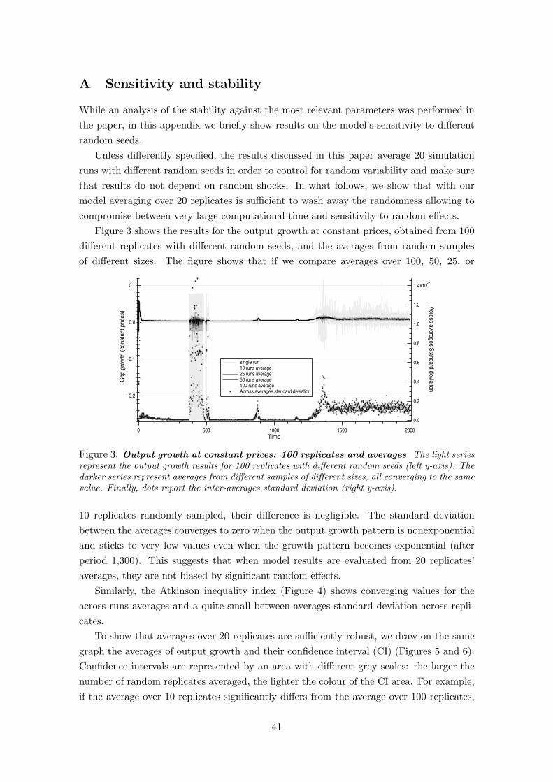
A Sensitivity and stability

While an analysis of the stability against the most relevant parameters was performed in

the paper, in this appendix we briefly show results on the model’s sensitivity to different

random seeds.

Unless differently specified, the results discussed in this paper average 20 simulation

runs with different random seeds in order to control for random variability and make sure

that results do not depend on random shocks. In what follows, we show that with our

model averaging over 20 replicates is sufficient to wash away the randomness allowing to

compromise between very large computational time and sensitivity to random effects.

Figure 3 shows the results for the output growth at constant prices, obtained from 100

different replicates with different random seeds, and the averages from random samples

of different sizes. The figure shows that if we compare averages over 100, 50, 25, or

-0.2

-0.1

0.0

0.1

Gdp g

row

th (

const

ant

price

s)

2000150010005000

Time

1.4x10-2

1.2

1.0

0.8

0.6

0.4

0.2

0.0

Across averages S

tandard deviaiton

single run 10 runs average 25 runs average 50 runs average 100 runs average Across averages standard deviation

Figure 3: Output growth at constant prices: 100 replicates and averages. The light seriesrepresent the output growth results for 100 replicates with different random seeds (left y-axis). Thedarker series represent averages from different samples of different sizes, all converging to the samevalue. Finally, dots report the inter-averages standard deviation (right y-axis).

10 replicates randomly sampled, their difference is negligible. The standard deviation

between the averages converges to zero when the output growth pattern is nonexponential

and sticks to very low values even when the growth pattern becomes exponential (after

period 1,300). This suggests that when model results are evaluated from 20 replicates’

averages, they are not biased by significant random effects.

Similarly, the Atkinson inequality index (Figure 4) shows converging values for the

across runs averages and a quite small between-averages standard deviation across repli-

cates.

To show that averages over 20 replicates are sufficiently robust, we draw on the same

graph the averages of output growth and their confidence interval (CI) (Figures 5 and 6).

Confidence intervals are represented by an area with different grey scales: the larger the

number of random replicates averaged, the lighter the colour of the CI area. For example,

if the average over 10 replicates significantly differs from the average over 100 replicates,

41

0.4

0.3

0.2

0.1

0.0

Atk

inso

n I

ndex

2000150010005000

Time

1.2x10-2

1.0

0.8

0.6

0.4

0.2

0.0

Sta

ndard

devia

tion

single run 10 runs average 25 runs average 50 runs average 100 runs average Standard deviation (across averages)

Figure 4: Atkinson inequality index: 100 replicates and averages. The light series rep-resent the results for 100 replicates with different random seeds (left y-axis). The darker seriesrepresent averages from different samples of different sizes, all converging to the same value (lefty-axis). Finally, dots report the inter-averages standard deviation (right y-axis).

one should see the confidence area of the 10 replicates average emerging below the white

CI. Otherwise, if the confidence areas of the 10 replicates’ averages are completely covered

by the lighter confidence area – of the 100 replicates average – we expect no significant

difference. When we compare the confidence area of an average of 100 independent random

!!∀

!!#∃

#!#∃

%&∋()∗+,−.(/−(0+12−/1−(∋∗3042(!(5∃6(7+183&4104(91−4∗:/;2

# ∃## ∀### ∀∃## <###

=3>4

=41−.(∀# =41−.(∀# ?31−.(∀# ?31−.(∀#

≅3).−(∀# ≅3).−(∀# Α4:41−.(∀# Α4:41−.(∀#

Α3Β−(∀# Α3Β−(∀# Χ38−.(∀# Χ38−.(∀#

Χ+∆∗−.(∀# Χ+∆∗−.(∀# =.3∗&(∀# =.3∗&(∀#

Α40+1&(∀# Α40+1&(∀# Χ3∗2−(∀# Χ3∗2−(∀#

Χ+∆∗−.(<∃ Χ+∆∗−.(<∃ =.3∗&(<∃ =.3∗&(<∃

Α40+1&(<∃ Α40+1&(<∃ Χ3∗2−(<∃ Χ3∗2−(<∃

Α40+1&(∃# Α40+1&(∃# Χ3∗2−(∃# Χ3∗2−(∃#

∀## ∀##

Figure 5: Output growth at constant prices: averages and confidence intervals. Thefigure shows the confidence areas of the different averages (over samples of 100, 50, 25, and 10replicates) superimposed one over the other, starting from 10 replicates’s averages. The grey scalegoes from dark grey for 10 replicates’ averages to white for the 100 replicates’ average. The figureshows that no section of the 10 replicates’ confidence area exceeds the 100 replicates’ confidencearea.

42

replicates with the confidence areas of 10 random averages from 10 independent subsamples

of replicates from the same 100 series, there is no difference in the CI of output growth

(Figure 5). None of the 10 average areas which lie below the 100 replicates confidence

area is visible. This allows us to infer that any 10 replicates’ average do not generate a

higher random variety than a 100 replicates average, and even less so if we average over

20 replicates.

When we perform the same exercise for the Atkinson inequality index, we obtain a

very similar result (Figure 6). The difference between the confidence areas is well below

one standard error. Overall, we feel confident that we can perform a robust analysis of

the model using averages over 20 different replicates, reducing by an exponential factor

the computational time needed to create averages for 100 different random seeds.

!∀!#

∀∃∀∃#

∀%

&∋()∗+,∗−)∗./012)∋3−)∗4.5−!−6#7−8,∗9)4.∗:.−;∗∋.<=12+

! #!! ∃!!! ∃#!! %!!!

>)?.

>.∗∋≅−∃! >.∗∋≅−∃!

Α)∗∋≅−∃! Α)∗∋≅−∃!

Β)Χ≅∋−∃! Β)Χ≅∋−∃!

∆.=.∗∋≅−∃! ∆.=.∗∋≅−∃!

∆)5∋−∃! ∆)5∋−∃!

Ε)9∋≅−∃! Ε)9∋≅−∃!

Ε,0<∋≅−∃! Ε,0<∋≅−∃!

>≅)<4−∃! >≅)<4−∃!

∆.:,∗4−∃! ∆.:,∗4−∃!

Ε)<+∋−∃! Ε)<+∋−∃!

Ε,0<∋≅−%# Ε,0<∋≅−%#

>≅)<4−%# >≅)<4−%#

∆.:,∗4−%# ∆.:,∗4−%#

Ε)<+∋−%# Ε)<+∋−%#

∆.:,∗4−#! ∆.:,∗4−#!

Ε)<+∋−#! Ε)<+∋−#!

∃!! ∃!!

Figure 6: Atkinson inequality index: averages and confidence intervals. The figure showsthe confidence areas of the different averages (over samples of 100, 50, 25, and 10 replicates)superimposed one over the other, starting from 10 replicates’ averages. The grey scale goes fromdark grey for 10 relicates’ averages to white for the 100 replicates average. The figure then showsthat very small sections of the 10 replicates’ confidence area exceed the 100 runs confidence area,amounting to a very small difference between the confidence areas of the different averages.

B Tables and Figures appendix

43

∆Y (200)/Y (1) Const. Obs.(1) ∆A(200)/A(1) 1.1905*** -0.0101*** 100

(0.1569) (0.0019)

∆Y (400)/Y (200) Const. Obs.(2) ∆A(400)/A(200) 0.0580 0.0002 100

(0.0796) (0.0003)

∆Y (600)/Y (400) Const. Obs.(3) ∆A(600)/A(400) -0.0149 7.5e-05 100

(0.0870) (0.0003)

∆Y (800)/Y (600) Const. Obs.(4) ∆A(800)/A(600) -0.1711 0.0007 100

(0.1690) (0.0007)

∆Y (1000)/Y (800) Const. Obs.(5) ∆A(1000)/A(800) 0.0112 -0.0001 100

(0.0503) (0.0003)

∆Y (1200)/Y (1000) Const. Obs.(6) ∆A(1200)/A(1000) 0.0605 -0.0003 100

(0.0415) (0.0002)

∆Y (1400)/Y (1200) Const. Obs.(7) ∆A(1400)/A(1200) 0.0880*** -1.4e-05 100

(0.0129) (0.0001)

∆Y (1600)/Y (1400) Const. Obs.(8) ∆A(1600)/A(1400) 0.1603*** -0.0008*** 100

(0.0079) (7.6e-05)

∆Y (1800)/Y (1600) Const. Obs.(9) ∆A(1800)/A(1600) 0.1675*** -0.0009*** 100

(0.0148) (0.0001)

∆Y (2000)/Y (1800) Const. Obs.(10) ∆A(2000)/A(1800) 0.1333*** 0.0007*** 100

(0.0225) (0.0002)

Standard errors in parentheses

*** p<0.01, ** p<0.05, * p<0.1

Least Absolute Deviation: Estimates computed using the Barrodale-Roberts simplex algorithm.

Standard errors derived using the bootstrap procedure with 500 drawings.

Table 11: Kaldor-Verdoorn Law Sub-Period Estimations. Least Absolute Deviation

44

(a) Average income (across populationand time)

(b) Total income from profit shares

Figure 7: Composition of production: initial product and preferences heterogeneityagainst income and profit shares. The figure shows the changes in the level of average incomeacross workers and time (a) as well as in the level of total income from profit shares (b) againstdifferent values of standard deviation of the product characteristics (x-axis) as well as againstchanging values of the difference between the minimum and maximum level of consumer tolerancetoward quality shortfalls with respect to the best firm.

45