Embed Size (px)
Citation preview
lable at ScienceDirect
Atmospheric Environment 89 (2014) 158e168
Contents lists avai
Atmospheric Environment
journal homepage: www.elsevier .com/locate/atmosenv
The role of temporal evolution in modeling atmospheric emissionsfrom tropical fires
Miriam E. Marlier a,*, Apostolos Voulgarakis b, Drew T. Shindell c, Greg Faluvegi c,Candise L. Henry a, James T. Randerson d
a Lamont-Doherty Earth Observatory and Dept. of Earth and Environmental Sciences at Columbia University, USAbDept. of Physics, Imperial College London, UKcNASA Goddard Institute for Space Studies, USAdDept. of Earth System Science, University of California, Irvine, USA
h i g h l i g h t s
� Daily and monthly resolution GFED fire emissions were modeled with GISS-E2-PUCCINI.� Simulations with daily resolution emissions were better timed with meteorology.� Effects on simulations of air quality exceedances and atmospheric heating patterns.
a r t i c l e i n f o
Article history:Received 8 October 2013Received in revised form14 February 2014Accepted 18 February 2014Available online 19 February 2014
Keywords:Fire emissionsAtmospheric modelingAir quality
* Corresponding author.E-mail addresses: [email protected], m
E. Marlier).
http://dx.doi.org/10.1016/j.atmosenv.2014.02.0391352-2310/� 2014 Elsevier Ltd. All rights reserved.
a b s t r a c t
Fire emissions associated with tropical land use change and maintenance influence atmosphericcomposition, air quality, and climate. In this study, we explore the effects of representing fire emissionsat daily versus monthly resolution in a global composition-climate model. We find that simulations ofaerosols are impacted more by the temporal resolution of fire emissions than trace gases such as carbonmonoxide or ozone. Daily-resolved datasets concentrate emissions from fire events over shorter timeperiods and allow them to more realistically interact with model meteorology, reducing how oftenemissions are concurrently released with precipitation events and in turn increasing peak aerosol con-centrations. The magnitude of this effect varies across tropical ecosystem types, ranging from smallerchanges in modeling the low intensity, frequent burning typical of savanna ecosystems to larger dif-ferences when modeling the short-term, intense fires that characterize deforestation events. The utilityof modeling fire emissions at a daily resolution also depends on the application, such as modelingexceedances of particulate matter concentrations over air quality guidelines or simulating regional at-mospheric heating patterns.
� 2014 Elsevier Ltd. All rights reserved.
1. Introduction
Fires are widely used throughout the tropics to create andmaintain areas for agricultural systems, but are also significantcontributors to atmospheric trace gas and aerosol concentrations(Andreae and Merlet, 2001). Emissions associated with deforesta-tion averaged 1 Pg carbon per year over the past decade (Bacciniet al., 2012), while also adding to atmospheric ozone (O3) pre-cursors such as carbon monoxide (CO), nitrogen oxides (NOx) andVOCs, sulfur-containing compounds, and particulates (Langmann
et al., 2009). In addition to the diversity in the type of emissions,the timing and magnitude of fire activity also varies interannuallyand by biome. This suggests that representing fire emissions atdifferent temporal resolutions in atmospheric models could alterinteractions between emissions and atmospheric chemistry andtransport, which also vary significantly on several timescales.
The tropics comprise a critical region for global fire activity, buthave varying fire behavior characteristics (van derWerf et al., 2010).Frequent but lower intensity fires are typical in savanna areas inAfrica and South America (van der Werf et al., 2010). Fire emissionsfrom Southern Hemisphere Africa are dominated by savannaburning, but the Amazon includes a mix of savanna and defores-tation fires, which leads to higher rates of fuel consumption andfewer fire days per year (when emissions are aggregated at a 0.5�
M.E. Marlier et al. / Atmospheric Environment 89 (2014) 158e168 159
spatial resolution). Equatorial Asia has even fewer average fire daysper year and higher daily rates of fuel consumption (Mu et al.,2011). On longer timescales, carbon-rich Equatorial Asian peat-land forest fires have higher interannual variability than other bi-omes (van der Werf et al., 2010), with large pulses of emissionsduring El Niño droughts (van der Werf et al., 2008). These regionaldifferences in emissions characteristics suggest that fire emissionsinventories with monthly resolution may be able to adequatelyresolve dominant modes of variability of fire behavior in certainbiomes, but could be insufficient in other areas. An importantchallenge for the atmospheric sciences community is to understandhow this variability in fire behavior influences chemistry, radiativeforcing, and air quality.
Monthly global gridded fire emissions inventories typicallycombine information from satellite observations of burned area,active fire detections, underlying vegetation characteristics, andmeteorology. One example is the Global Fire Emissions Databaseversion 3 (GFED3), which is available at a monthly resolution from1997 to 2011 (van der Werf et al., 2010). From November 2000onwards, it detects changes in 500-mModerate Resolution ImagingSpectroradiometer (MODIS) surface reflectance and 1-km MODISactive fires to inform an automated hybrid burned area mappingalgorithm (Giglio et al., 2009). Before 2000, active fire detectionsfrom Tropical Rainfall Measuring Mission (TRMM) Visible andInfrared Scanner (VIRS) and the Along-Track Scanning Radiometer(ATSR) are used to estimate burned area by means of a regressionwith MODIS burned area during overlap periods, which necessi-tates the dataset’s monthly resolution (Giglio et al., 2010). Duncanet al. (2003) used active fire data from ATSR and the AdvancedVery High Resolution Radiometer (AVHRR) to estimate seasonal firevariability, with the Total Ozone Mapping Spectrometer (TOMS)Aerosol Index serving as a proxy for interannual variability inselected regions, which then scaled an existing biomass burninginventory. While these datasets capture important information onseasonal and interannual variability in fire activity, they may haveimportant limitations when implemented into modeling systemswhich otherwise operate at sub-daily increments.
Recognizing these potential limitations, several fire emissionsinventories at daily or sub-daily resolution are also available, usingsatellite active fire detections to represent emissions at a finertemporal resolution. Mu et al. (2011) recently applied active firecounts from MODIS and the Geostationary Operational Environ-mental Satellite (GOES) Wildfire Automated Biomass Burning Al-gorithm (WF_ABBA) to create daily and 3-hourly emissionsinventories, respectively, from the original GFED3 monthly dataset.Heald et al. (2003) applied AVHRR active fire observations to theDuncan et al. (2003) inventory to create a daily emissions datasetfor early 2001. The Fire Inventory from NCAR (FINN) is a daily 1-kmglobal dataset of trace gas and particulate emissions from fires,available from 2005 to 10 (Wiedinmyer et al., 2011). FINN primarilyuses MODIS active fire detections, an assumed burned area perdetection (to allow the product to be released close to real-time),and MODIS land cover types to estimate fuel loadings. FireLocating and Modeling of Burning Emissions (FLAMBE) combinesGOES WF_ABBA, near real-time MODIS active fire products, and 1-km AVHRR land cover maps to create hourly emissions inventories,from 2005 onwards (Reid et al., 2009). Kaiser et al. (2012) devel-oped the 0.5 � 0.5� Global Fire Assimilation System (GFASv1.0),available from 2003, by calculating biomass burning emissionsbased on MODIS fire radiative power and land cover-specificcombustion factors derived from the GFED3 emissions inventory.
Many daily or sub-daily emissions products rely on MODISactive fire detections and are therefore only available since late2002, when both Terra and Aqua were in operation together.Therefore, for modeling studies before the MODIS era, monthly
inventories may still be the only option. Some chemical transportmodels are moving towards using daily or hourly fire emissions(Mu et al., 2011), althoughmost global composition-climate modelscurrently implement monthly resolution emissions (Lee et al.,2013). It remains unclear which aspects of atmospheric modelingare most sensitive to this choice of temporal resolution, because inprevious studies, using finer temporal resolution emissions overcoarser resolution datasets have offered variable improvementswhen compared with observations. Model simulations focusing onCO have found improvements with daily over monthly fire emis-sions but not sub-daily resolution emissions (Mu et al., 2011),monthly over climatological, but not daily (Heald et al., 2003), and8-day instead of monthly, but not diurnal (Chen et al., 2009).Simulations of shorter-lived species like NO2 improve from sub-daily emissions that capture the afternoon peak of biomassburning emissions (Boersma et al., 2008). In boreal North America,Chen et al. (2009) found that aerosols were more sensitive to using8-day versus monthly resolution emissions thanwas foundwith CO(also without further improvements with diurnal resolution). Inareas such as Singapore, where biomass burning aerosol transportfrom Indonesia is highly variable over the fire season, both withrespect to shifts in geographic patterns of burning and atmospherictransport patterns, detailed temporal resolution of fire emissionsinventories may improve modeled regional aerosol concentrations(Atwood et al., 2013). Modeling the interactions between smokeaerosols by changing absorption patterns of radiation can also varystrongly on sub-daily timescales (Wang and Christopher, 2006; Wuet al., 2011).
In this study, we examine the sensitivity of multiple endpointsto using daily and monthly resolution fire emissions: modelingtrace gases and aerosols, assessing air quality and public healtheffects, and estimating climate impacts. We hypothesize thatchanging from monthly to daily fire emissions will: 1) produce avaried response throughout the tropics, depending on biome-specific fire behavior (for example, continuous low intensity fireswould lead to smaller atmospheric differences in savanna regions),2) allow for higher peak concentrations since short-lived fire eventscan be concentrated over several days and not averaged over amonth, and 3) more realistically synchronize emissions withmeteorology, with fires predominately occurring on sunny,precipitation-free days, which would lower wet deposition ofaerosols and could increase the speed of some chemical reactions.Section 2 describes the model framework and observational data-sets; Section 3 presents our results for atmospheric composition,air quality, and radiative forcing; Section 4 describes ourconclusions.
2. Materials and methods
2.1. Model set-up
Baseline monthly fire emissions estimates were from GFED3,which combines surface reflectance and active fire detections fromseveral satellites to detect the spatiotemporal variability of burnedarea (Giglio et al., 2010). This drives a biogeochemical model thatestimates fuel loads, combustion completeness, and emissions (vander Werf et al., 2010). GFED3 is available for 1997 onwards at0.5� � 0.5� horizontal resolution. This dataset comprised the fireinput for our monthly fire emissions (MF) run.
To isolate the influence of the temporal resolution of fireemissions instead of variations among fire emissions inventories,we used a daily emissions dataset with the same bulk total emis-sions as the monthly GFED3 dataset. Mu et al. (2011) used MODISactive fire detections aboard the Terra and Aqua satellites to parsethe monthly GFED3 emissions to a daily resolution. Due to gaps in
M.E. Marlier et al. / Atmospheric Environment 89 (2014) 158e168160
satellite overpasses in the tropics, they applied a three daysmoothing filter between 25�N and 25�S. This dataset comprisedour daily fire emissions (DF) run. Both fire emissions datasets arepublicly available (http://www.globalfiredata.org). We did notinclude diurnal variability in fire emissions.
Simulations were run with GISS-E2-PUCCINI, which is the latestversion of the NASA GISS ModelE climate model, including inter-active chemistry and aerosols (Shindell et al., 2013b). Following atwo year spin-up, it was run at 2� � 2.5� resolution with 40 verticallayers from 2005 to 2009. We conducted three simulations: 1) MF,2) DF, and 3) NF (no fire emissions).
Our simulations included interactive constituents in the PUC-CINI model for chemistry, aerosols (sulfate, carbonaceous, nitrate,dust and sea salt), and an aerosol indirect effect parameterization(Koch et al., 2006; Shindell et al., 2013b). GFED3 emissions weremixed uniformly through the boundary layer. Infrastructure hasrecently been developed in the PUCINNI model to study pulses ofemissions from individual fire events and preliminary resultsshow satisfactory performance compared with observations(Robert Field, personal communication). Monthly emissions werelinearly interpolated to daily values for the MF simulation whilethe daily fractions from the Mu et al. (2011) product were used forthe DF simulation. Annually and monthly-varying GFED3 emis-sions were used for CO, ammonia, black carbon (BC), organiccarbon (OC), sulfur dioxide, non-methane hydrocarbons, and NOx.To isolate the difference between DF and MF, we did not scaleaerosol emissions by satellite observations. Present-day anthro-pogenic emissions were re-gridded to 2� � 2.5� spatial resolutionbased on Lamarque et al. (2010), which was produced to provide
Table 1Description of ground-based validation data for intercomparison with model simulationNetwork, AOD ¼ Aerosol Optical Depth, SHSA¼Southern Hemisphere South America, Sbeginning and ending dates, irrespective of gaps.
Source Species Region
WDCGG CO SHSACO, O3 SHSAO3 SHSACO, O3 SHAF
CO, O3 SHAF
CO SHAFCO, O3 EQAS
O3 EQASAERONET AOD SHSA
AOD SHAF
AOD EQAS
input to models being run in support of the IPCC Fifth AssessmentReport (AR5). Methane in the lowest model layer was kept toobserved values for each year and lightning NOx was generatedinternally based on an updated version of Price et al. (1997).Climate-sensitive isoprene emissions were based on Guentheret al. (1995, 2006); vegetation alkene and paraffin emissionsfrom the GEIA dataset are based on Guenther et al. (1995). Modelwinds were linearly relaxed towards reanalysis based on meteo-rological observations (Rienecker et al., 2011). Sea-surface tem-peratures and sea ice were from monthly observational datasets(Rayner et al., 2003).
We focused on several key trace gases and aerosol species toillustrate the changes between the DF and MF simulations. Tracegases included CO, O3, and OH to understand how the modelsimulates atmospheric composition; both O3 and CO are majorpollutants, while O3 and OH are also directly and indirectlyimportant, respectively, to climate. For aerosols, we focused on BCand OC, which are the main components of particulate matter towhich fire emissions contribute (Andreae and Merlet, 2001).
2.2. Ground and satellite observations
We compared model output with ground-based (Table 1) andsatellite measurements of O3, CO, and aerosol optical depth (AOD).Observations were generally selected within primary tropical fireregions as defined in by GFED (van der Werf et al., 2010): SouthernHemisphere South America, Southern Hemisphere Africa, andEquatorial Asia, although we expanded the regions slightlydepending on station coverage. Of the 14 GFED regions, these three
s. WDCGG¼ World Data Centre for Greenhouse Gases, AERONET ¼ Aerosol RoboticHAF¼Southern Hemisphere Africa, EQAS ¼ Equatorial Asia. Time period lists data
Location (latitude, longitude) Time period
Arembepe, Brazil (�12.8, �38.2) 10/2006e12/2009Ushuaia, Argentina (�54.8, �68.3) 3/2005e1/2009San Lorenzo, Paraguay (�25.4, �57.6) 3/2005e10/2007Cape Point, South Africa (�34.4, 18.5) CO: 1/2007e12/2009
O3: 1/2005e12/2009Mt. Kenya, Kenya (�0.1, 37.3) CO: 1/2005e5/2006
O3: 3/2005e5/2006Gobabeb, Namibia (�23.6, 15.0) 8/2006e12/2009Bukit Koto Tabang, Indonesia(-0.2, 100.3)
CO: 1/2005e12/2009O3: 1/2005e12/2007
Danum Valley, Malaysia (5.0, 117.8) 1/2007e5/2008Abracos Hill (�10.8, �62.4) 1/2005e10/2005Alta Floresta (�9.9, �56.1) 1/2005e12/2009Belterra (�2.6, �55.0) 1/2005e4/2005Campo Grande (�20.4, �54.5) 1/2005e12/2009Cuiba Miranda (�15.7, �56.0) 1/2005e6/2009Petrolina Sonda (�9.4, �40.5) 1/2005e9/2009Rio Branco (�10.0, �67.9) 1/2005e12/2009Santa Cruz (�17.8, �63.2) 2/2005e12/2009Santa Cruz Utepsa (�17.9, �63.2) 9/2006e11/2008Sao Paulo (�23.6, �46.7) 1/2005e12/2009ICIPE-Mbita (�0.4, 34.2) 3/2006e8/2008Ilorin (8.3, 4.3) 1/2005e12/2009Kibale (0.6, 30.4) 12/2006e1/2007Mongu (�15.3, 23.2) 1/2005e12/2009Nairobi (�1.3, 36.9) 12/2005e6/2009Niamey (13.5, 2.2) 8/2006e1/2007Skukuza (�25.0, 31.6) 1/2005e12/2009Jabiru (�12.7, 132.9) 5/2005e12/2009Bandung (�6.9, 107.6) 5/2009e12/2009Puspiptek (�6.4, 106.7) 8/2007e11/2007Singapore (1.3, 103.8) 11/2006e12/2009Bac Lieu (9.3, 105.7) 5/2006e7/2009ND Marbel University (6.5, 124.8) 12/2009Songkhla (7.2, 100.6) 1/2007e12/2009
M.E. Marlier et al. / Atmospheric Environment 89 (2014) 158e168 161
contributed more than 50% of global emissions over 2005e2009(van der Werf et al., 2010).
The World Data Centre for Greenhouse Gases (WDCGG) main-tains station trace gas observations (http://ds.data.jma.go.jp/gmd/wdcgg/). We used 24-h averages of surface O3 and CO concentra-tions for comparison with surface model output. As described inTable 1, CO and/or O3 data were available from 8 stations for vari-able time periods within 2005e2009.
NASA’s AErosol RObotic NETwork (AERONET) is a global ground-based sun photometer network (http://aeronet.gsfc.nasa.gov)(Holben et al., 1998). Column AOD is calculated from direct solarradiationmeasurements. We used Version 2, Level 2.0 24-h averagedata, which is the highest quality screened product available. Therewere 24 available stations (Table 1).
We also compared modeled AOD with MODIS and Multi-angleImaging SpectroRadiometer (MISR) daily satellite AOD products.We averaged modeled instantaneous AOD values for 12pm and3pm to correspond with the 1:30pm Aqua satellite overpass forMODIS and 9am to 12pm to correspond with the 10:30am Terrasatellite overpass for MISR. AOD retrievals from MODIS takeadvantage of a wide spectral range, daily coverage of the globe, andhigh spatial resolution. We used the daily MODIS 1� � 1� Level 3,Collection 5 monthly AOD (MOD08 D3) product (http://modis.gsfc.nasa.gov). MISR (http://www-misr.jpl.nasa.gov) simultaneouslyobserves the Earth at nine different angles and four spectral bands,with global coverage every nine days at the equator. We used thegridded 0.5� � 0.5� Level 3 daily AOD product (MIL3DAE) from thegreen (555 nm) band.
2.3. Air quality
The World Health Organization (WHO) combines results fromepidemiological studies on the public health risks of air pollutantsand publishes air quality guidelines (World Health Organization,2006). These guidelines serve as goals for countries to improveair quality, and are published along with higher interim targetslevels (ITs) that have additional expected health risks. We exam-ined how modeling population exposure in the tropics changedwith DF versus MF by testing changes in peak concentrationsthrough exceedances over 24-h and annual PM2.5 and 8-hmaximum O3 ITs.
Annual cardiovascular disease (CVD) mortality burdens wereestimated for exposure to fire PM2.5 with a powerelaw relationshipthat describes how relative risk (RR) changes over a baseline valueof 1:
RR ¼ 1þ aðI*CÞb (1)
We used published values for a and b from a reanalysis ofstudies that include exposure to ambient air pollution, second-hand smoke, and cigarette smoke. For CVD disease, a ¼ 0.2685and b ¼ 0.2730 (Pope et al., 2011). Annual average total mass PM2.5surface concentrations were used for (C), assuming a constantaverage inhalation rate (I) of 18 m3/day to convert to PM2.5 dose (inmg). The attributable fraction (AF) and annual mortality (DM) wereestimated by Ostro (2004):
AF ¼ ðRR � 1Þ=RR (2)
DMannual ¼ M�bP�
�AFfire � AFnofire
�(3)
where the average annual baseline mortality rate (Mb) was calcu-lated from adult deaths due to cardiovascular disease, averagedover the countries within each region (WHO, 2011). The fraction ofpeople over 30 years was from the UN Population Division (UN,
2011) and baseline population was from CIESIN’s Gridded Popula-tion of the World version 3 for 2005 (CIESIN, 2005a) and FutureEstimates for 2010 (CIESIN, 2005b); both the adult fraction andpopulation were linearly interpolated from 5 yearly to annual es-timates. In addition, we estimated themortality burden due to dailyexposure to fire emissions, summed over each year. Here we used alinear concentration-response function between all-cause mortal-ity and PM10 exposure (0.8% per 10 mg/m3 increase in PM10) with anupper effect threshold of 125 mg/m3 (Ostro, 2004).We assumed thatthe annual mortality rates described previously were evenly spreadover the year.
2.4. Radiative forcing
To evaluate the potential climate implications of our results, wecalculated differences between surface and top-of-atmosphere(TOA) instantaneous long-wave and shortwave radiative forcingfor several constituents affected by biomass burning. Radiativeforcing, inW/m2, was evaluated for BC, O3, and sulfate (SO4) in eachsimulation, as these are the most radiatively active species that areaffected by fires. Radiative forcing was calculated online as anaverage over time during the simulations; calculations were per-formed twice at each point in time, with the only difference in thetwo calculations being the constituent field (e.g. BC, O3, etc.). Theradiative forcing calculations follow standardmethodology that hasbeen used in previous workwith the PUCCINI model (Shindell et al.,2013b; Voulgarakis et al., 2013b).
3. Results
3.1. Atmospheric composition
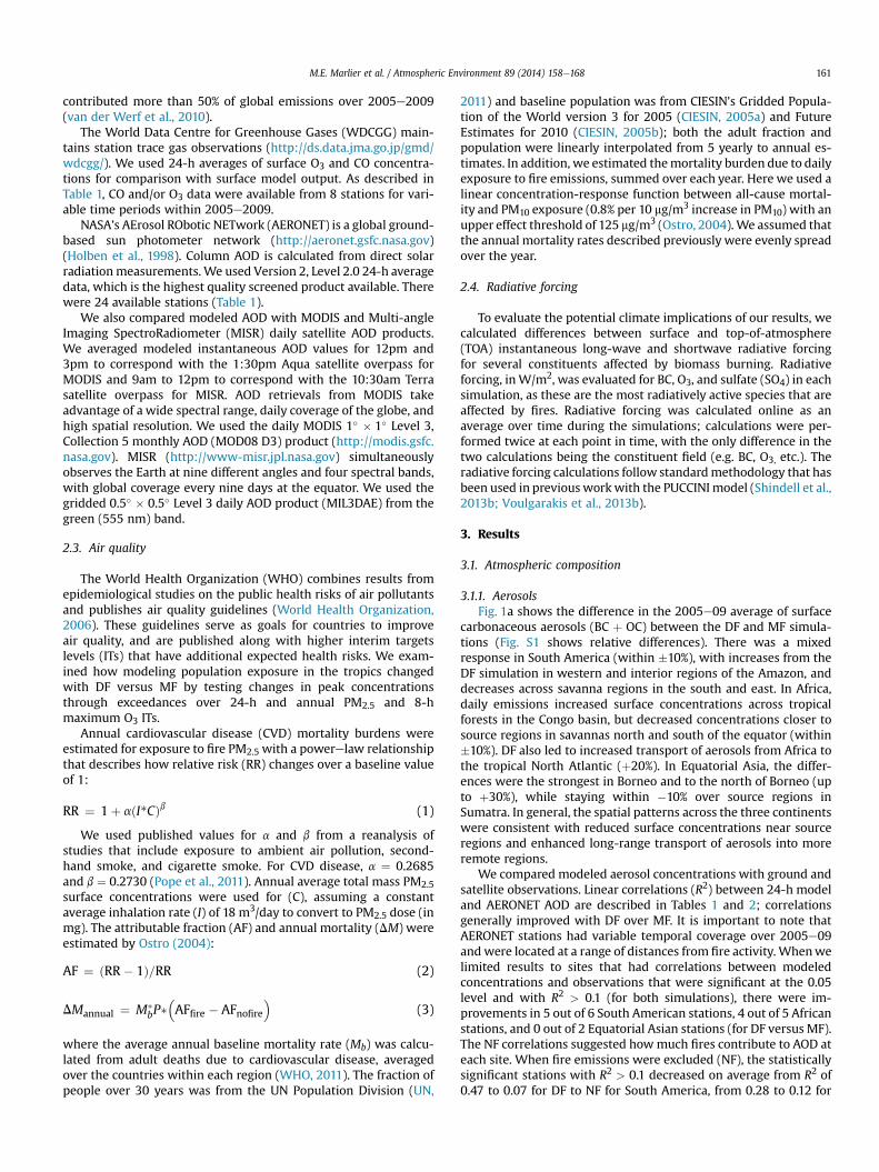
3.1.1. AerosolsFig. 1a shows the difference in the 2005e09 average of surface
carbonaceous aerosols (BC þ OC) between the DF and MF simula-tions (Fig. S1 shows relative differences). There was a mixedresponse in South America (within �10%), with increases from theDF simulation in western and interior regions of the Amazon, anddecreases across savanna regions in the south and east. In Africa,daily emissions increased surface concentrations across tropicalforests in the Congo basin, but decreased concentrations closer tosource regions in savannas north and south of the equator (within�10%). DF also led to increased transport of aerosols from Africa tothe tropical North Atlantic (þ20%). In Equatorial Asia, the differ-ences were the strongest in Borneo and to the north of Borneo (upto þ30%), while staying within �10% over source regions inSumatra. In general, the spatial patterns across the three continentswere consistent with reduced surface concentrations near sourceregions and enhanced long-range transport of aerosols into moreremote regions.
We compared modeled aerosol concentrations with ground andsatellite observations. Linear correlations (R2) between 24-h modeland AERONET AOD are described in Tables 1 and 2; correlationsgenerally improved with DF over MF. It is important to note thatAERONET stations had variable temporal coverage over 2005e09andwere located at a range of distances from fire activity. Whenwelimited results to sites that had correlations between modeledconcentrations and observations that were significant at the 0.05level and with R2 > 0.1 (for both simulations), there were im-provements in 5 out of 6 South American stations, 4 out of 5 Africanstations, and 0 out of 2 Equatorial Asian stations (for DF versus MF).The NF correlations suggested howmuch fires contribute to AOD ateach site. When fire emissions were excluded (NF), the statisticallysignificant stations with R2 > 0.1 decreased on average from R2 of0.47 to 0.07 for DF to NF for South America, from 0.28 to 0.12 for
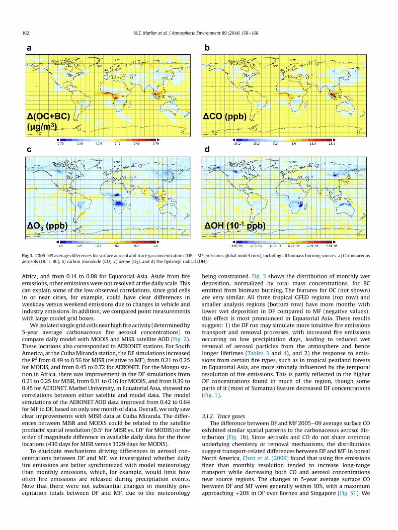
Fig. 1. 2005e09 average differences for surface aerosol and trace gas concentrations (DF eMF emissions global model runs), including all biomass burning sources. a) Carbonaceousaerosols (OC þ BC), b) carbon monoxide (CO), c) ozone (O3), and d) the hydroxyl radical (OH).
M.E. Marlier et al. / Atmospheric Environment 89 (2014) 158e168162
Africa, and from 0.14 to 0.08 for Equatorial Asia. Aside from fireemissions, other emissions were not resolved at the daily scale. Thiscan explain some of the low observed correlations, since grid cellsin or near cities, for example, could have clear differences inweekday versus weekend emissions due to changes in vehicle andindustry emissions. In addition, we compared point measurementswith large model grid boxes.
We isolated singlegrid cells nearhighfireactivity (determinedby5-year average carbonaceous fire aerosol concentrations) tocompare daily model with MODIS and MISR satellite AOD (Fig. 2).These locations also corresponded to AERONET stations. For SouthAmerica, at the CuibaMiranda station, the DF simulations increasedthe R2 from 0.49 to 0.56 for MISR (relative to MF), from 0.21 to 0.25for MODIS, and from 0.45 to 0.72 for AERONET. For the Mongu sta-tion in Africa, there was improvement in the DF simulations from0.21 to 0.25 for MISR, from 0.11 to 0.16 for MODIS, and from 0.39 to0.45 for AERONET. Marbel University, in Equatorial Asia, showed nocorrelations between either satellite and model data. The modelsimulations of the AERONET AOD data improved from 0.42 to 0.64for MF to DF, based on only onemonth of data. Overall, we only sawclear improvements with MISR data at Cuiba Miranda. The differ-ences between MISR and MODIS could be related to the satelliteproducts’ spatial resolution (0.5� for MISR vs. 1.0� for MODIS) or theorder of magnitude difference in available daily data for the threelocations (430 days for MISR versus 3329 days for MODIS).
To elucidate mechanisms driving differences in aerosol con-centrations between DF and MF, we investigated whether dailyfire emissions are better synchronized with model meteorologythan monthly emissions, which, for example, would limit howoften fire emissions are released during precipitation events.Note that there were not substantial changes in monthly pre-cipitation totals between DF and MF, due to the meteorology
being constrained. Fig. 3 shows the distribution of monthly wetdeposition, normalized by total mass concentrations, for BCemitted from biomass burning. The features for OC (not shown)are very similar. All three tropical GFED regions (top row) andsmaller analysis regions (bottom row) have more months withlower wet deposition in DF compared to MF (negative values);this effect is most pronounced in Equatorial Asia. These resultssuggest: 1) the DF run may simulate more intuitive fire emissionstransport and removal processes, with increased fire emissionsoccurring on low precipitation days, leading to reduced wetremoval of aerosol particles from the atmosphere and hencelonger lifetimes (Tables 3 and 4), and 2) the response to emis-sions from certain fire types, such as in tropical peatland forestsin Equatorial Asia, are more strongly influenced by the temporalresolution of fire emissions. This is partly reflected in the higherDF concentrations found in much of the region, though someparts of it (most of Sumatra) feature decreased DF concentrations(Fig. 1).
3.1.2. Trace gasesThe difference between DF and MF 2005e09 average surface CO
exhibited similar spatial patterns to the carbonaceous aerosol dis-tribution (Fig. 1b). Since aerosols and CO do not share commonunderlying chemistry or removal mechanisms, the distributionssuggest transport-related differences between DF and MF. In borealNorth America, Chen et al. (2009) found that using fire emissionsfiner than monthly resolution tended to increase long-rangetransport while decreasing both CO and aerosol concentrationsnear source regions. The changes in 5-year average surface CObetween DF and MF were generally within 10%, with a maximumapproaching þ20% in DF over Borneo and Singapore (Fig. S1). We
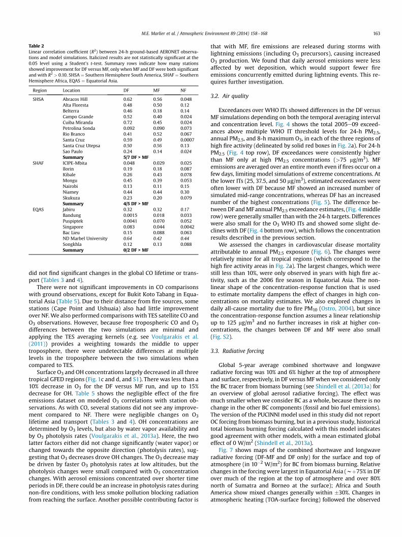
Table 2Linear correlation coefficient (R2) between 24-h ground-based AERONET observa-tions and model simulations. Italicized results are not statistically significant at the0.05 level using a Student’s t-test. Summary rows indicate how many stationsshowed improvement for DF versus MF, only when MF and DF were both significantand with R2 > 0.10. SHSA ¼ Southern Hemisphere South America, SHAF ¼ SouthernHemisphere Africa, EQAS ¼ Equatorial Asia.
Region Location DF MF NF
SHSA Abracos Hill 0.62 0.56 0.048Alta Floresta 0.48 0.50 0.12Belterra 0.46 0.18 0.14Campo Grande 0.52 0.40 0.024Cuiba Miranda 0.72 0.45 0.024Petrolina Sonda 0.092 0.090 0.073Rio Branco 0.41 0.52 0.067Santa Cruz 0.59 0.49 0.0007Santa Cruz Utepsa 0.50 0.56 0.13Sao Paulo 0.24 0.14 0.024Summary 5/7 DF > MF
SHAF ICIPE-Mbita 0.048 0.029 0.025Ilorin 0.19 0.18 0.087Kibale 0.26 0.43 0.078Mongu 0.45 0.39 0.053Nairobi 0.13 0.11 0.15Niamey 0.44 0.44 0.30Skukuza 0.23 0.20 0.079Summary 4/5 DF > MF
EQAS Jabiru 0.32 0.32 0.17Bandung 0.0015 0.018 0.033Puspiptek 0.0041 0.070 0.052Singapore 0.083 0.044 0.0042Bac Lieu 0.15 0.088 0.063ND Marbel University 0.64 0.42 0.44Songkhla 0.12 0.13 0.088Summary 0/2 DF > MF
M.E. Marlier et al. / Atmospheric Environment 89 (2014) 158e168 163
did not find significant changes in the global CO lifetime or trans-port (Tables 3 and 4).
There were not significant improvements in CO comparisonswith ground observations, except for Bukit Koto Tabang in Equa-torial Asia (Table 5). Due to their distance from fire sources, somestations (Cape Point and Ushuaia) also had little improvementover NF. We also performed comparisons with TES satellite CO andO3 observations. However, because free tropospheric CO and O3differences between the two simulations are minimal andapplying the TES averaging kernels (e.g. see Voulgarakis et al.(2011)) provides a weighting towards the middle to uppertroposphere, there were undetectable differences at multiplelevels in the troposphere between the two simulations whencompared to TES.
Surface O3 and OH concentrations largely decreased in all threetropical GFED regions (Fig. 1c and d, and S1). There was less than a10% decrease in O3 for the DF versus MF run, and up to 15%decrease for OH. Table 5 shows the negligible effect of the fireemissions dataset on modeled O3 correlations with station ob-servations. As with CO, several stations did not see any improve-ment compared to NF. There were negligible changes on O3lifetime and transport (Tables 3 and 4). OH concentrations aredetermined by O3 levels, but also by water vapor availability andby O3 photolysis rates (Voulgarakis et al., 2013a). Here, the twolatter factors either did not change significantly (water vapor) orchanged towards the opposite direction (photolysis rates), sug-gesting that O3 decreases drove OH changes. The O3 decrease maybe driven by faster O3 photolysis rates at low altitudes, but thephotolysis changes were small compared with O3 concentrationchanges. With aerosol emissions concentrated over shorter timeperiods in DF, there could be an increase in photolysis rates duringnon-fire conditions, with less smoke pollution blocking radiationfrom reaching the surface. Another possible contributing factor is
that with MF, fire emissions are released during storms withlightning emissions (including O3 precursors), causing increasedO3 production. We found that daily aerosol emissions were lessaffected by wet deposition, which would support fewer fireemissions concurrently emitted during lightning events. This re-quires further investigation.
3.2. Air quality
Exceedances over WHO ITs showed differences in the DF versusMF simulations depending on both the temporal averaging intervaland concentration level. Fig. 4 shows the total 2005e09 exceed-ances above multiple WHO IT threshold levels for 24-h PM2.5,annual PM2.5, and 8-h maximum O3, in each of the three regions ofhigh fire activity (delineated by solid red boxes in Fig. 2a). For 24-hPM2.5 (Fig. 4 top row), DF exceedances were consistently higherthan MF only at high PM2.5 concentrations (>75 mg/m3). MFemissions are averaged over an entiremonth even if fires occur on afew days, limiting model simulations of extreme concentrations. Atthe lower ITs (25, 37.5, and 50 mg/m3), estimated exceedances wereoften lower with DF because MF showed an increased number ofsimulated mid-range concentrations, whereas DF has an increasednumber of the highest concentrations (Fig. 5). The difference be-tween DF andMFannual PM2.5 exceedance estimates, (Fig. 4 middlerow) were generally smaller thanwith the 24-h targets. Differenceswere also small for the O3 WHO ITs and showed some slight de-clines with DF (Fig. 4 bottom row), which follows the concentrationresults described in the previous section.
We assessed the changes in cardiovascular disease mortalityattributable to annual PM2.5 exposure (Fig. 6). The changes wererelatively minor for all tropical regions (which correspond to thehigh fire activity areas in Fig. 2a). The largest changes, which werestill less than 10%, were only observed in years with high fire ac-tivity, such as the 2006 fire season in Equatorial Asia. The non-linear shape of the concentration-response function that is usedto estimate mortality dampens the effect of changes in high con-centrations on mortality estimates. We also explored changes indaily all-cause mortality due to fire PM10 (Ostro, 2004), but sincethe concentration-response function assumes a linear relationshipup to 125 mg/m3 and no further increases in risk at higher con-centrations, the changes between DF and MF were also small(Fig. S2).
3.3. Radiative forcing
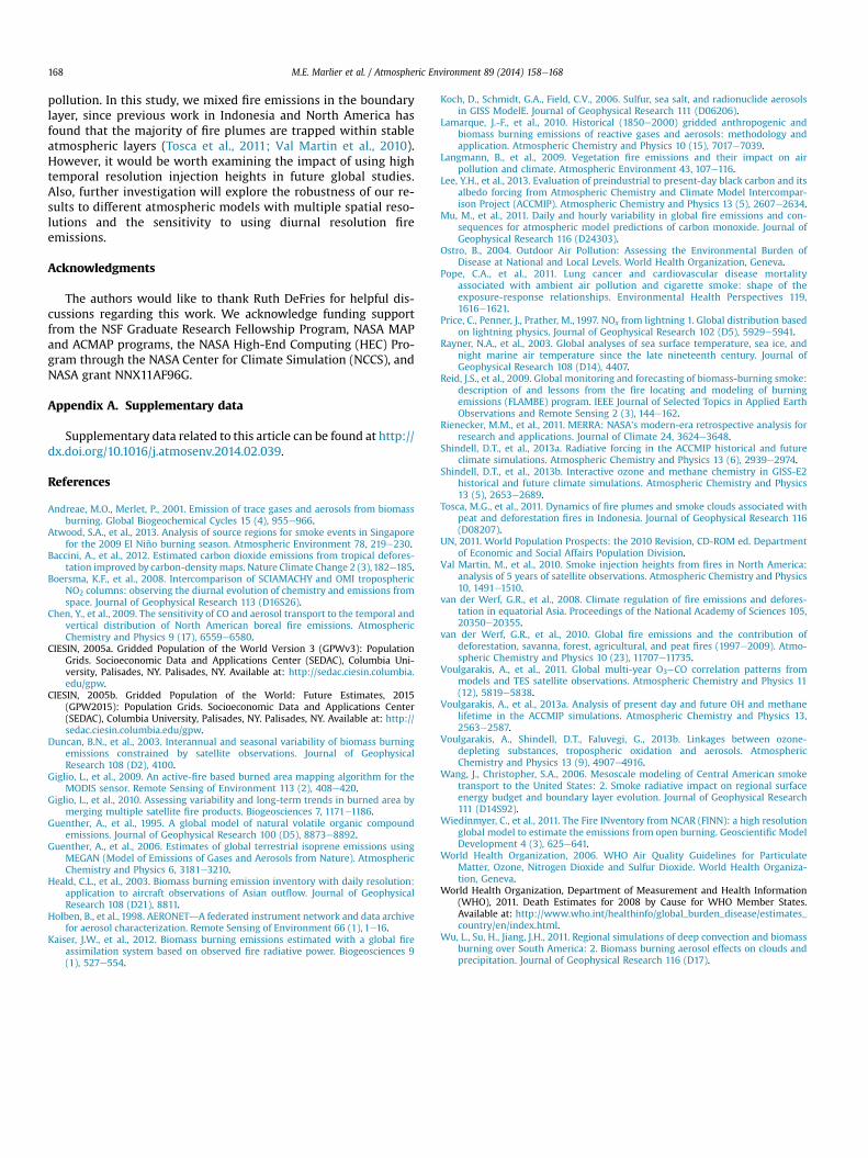
Global 5-year average combined shortwave and longwaveradiative forcing was 10% and 6% higher at the top of atmosphereand surface, respectively, in DF versus MFwhenwe considered onlythe BC tracer from biomass burning (see Shindell et al. (2013a) foran overview of global aerosol radiative forcing). The effect wasmuch smaller whenwe consider BC as a whole, because there is nochange in the other BC components (fossil and bio fuel emissions).The version of the PUCINNI model used in this study did not reportOC forcing from biomass burning, but in a previous study, historicaltotal biomass burning forcing calculated with this model indicatesgood agreement with other models, with a mean estimated globaleffect of 0 W/m2 (Shindell et al., 2013a).
Fig. 7 shows maps of the combined shortwave and longwaveradiative forcing (DF-MF and DF only) for the surface and top ofatmosphere (in 10�2 W/m2) for BC from biomass burning. Relativechanges in the forcingwere largest in Equatorial Asia (wþ75% in DFover much of the region at the top of atmosphere and over 80%north of Sumatra and Borneo at the surface); Africa and SouthAmerica show mixed changes generally within �30%. Changes inatmospheric heating (TOA-surface forcing) followed the observed
Fig. 2. a) Regions of analysis for model-data intercomparisons. Locations for comparisons of model AOD with MODIS and MISR satellite AOD observations (black stars), GFED basisregions (dotted black boxes) and small target regions for analysis (solid red boxes). Underlying map shows the 2005e09 average carbonaceous surface aerosol concentrations due tofires only, using daily fire emissions. b) Daily mean satellite AOD (MODIS, top row, and MISR, bottom row) versus modeled AOD for 2005e2009. (For interpretation of the referencesto colour in this figure legend, the reader is referred to the web version of this article.)
M.E. Marlier et al. / Atmospheric Environment 89 (2014) 158e168164
TOA patterns (maps not shown). There was little change (w1%) inhemispheric or global O3 forcing and no change in SO4 forcing.
4. Discussion
We observed both increases and decreases of aerosol concen-trations in response to changing the temporal resolution of fireemissions, though the changes generally support our three hy-potheses. Comparedwith ground-based AERONETobservations, we
found that correlations between simulated and observed AOD tendto improve with DF over MF (Table 2), but found less improvementwhen model simulations were compared with satellite AOD. Im-provements were more pronounced in South America and Equa-torial Asia than savanna-dominated Southern Hemisphere Africa,which is expected from the ability of DF to capture fire events thatare concentrated over several days in these biomes. Analysis intothe mechanism behind these changes lends support to our hy-pothesis that the daily fire emissions are better timed with
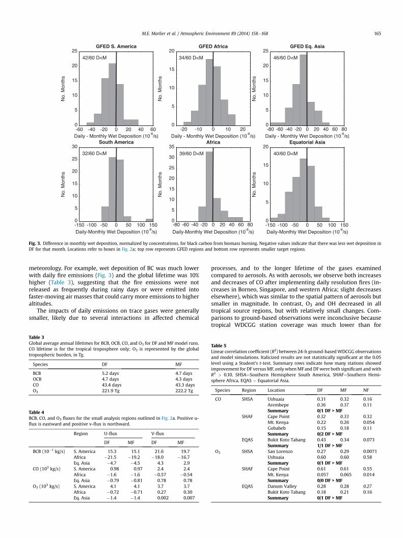
Fig. 3. Difference in monthly wet deposition, normalized by concentrations, for black carbon from biomass burning. Negative values indicate that there was less wet deposition inDF for that month. Locations refer to boxes in Fig. 2a; top row represents GFED regions and bottom row represents smaller target regions.
M.E. Marlier et al. / Atmospheric Environment 89 (2014) 158e168 165
meteorology. For example, wet deposition of BC was much lowerwith daily fire emissions (Fig. 3) and the global lifetime was 10%higher (Table 3), suggesting that the fire emissions were notreleased as frequently during rainy days or were emitted intofaster-moving air masses that could carry more emissions to higheraltitudes.
The impacts of daily emissions on trace gases were generallysmaller, likely due to several interactions in affected chemical
Table 3Global average annual lifetimes for BCB, OCB, CO, and O3 for DF and MF model runs.CO lifetime is for the tropical troposphere only; O3 is represented by the globaltropospheric burden, in Tg.
Species DF MF
BCB 5.2 days 4.7 daysOCB 4.7 days 4.3 daysCO 43.4 days 43.3 daysO3 221.9 Tg 222.2 Tg
Table 4BCB, CO, and O3 fluxes for the small analysis regions outlined in Fig. 2a. Positive u-flux is eastward and positive v-flux is northward.
Region U-flux V-flux
DF MF DF MF
BCB (10�1 kg/s) S. America 15.3 15.1 21.6 19.7Africa �21.5 �19.2 �18.0 �16.7Eq. Asia �4.7 �4.5 4.3 2.9
CO (103 kg/s) S. America 0.98 0.97 2.4 2.4Africa �1.6 �1.6 �0.57 �0.54Eq. Asia �0.79 �0.81 0.78 0.78
O3 (103 kg/s) S. America 4.1 4.1 3.7 3.7Africa �0.72 �0.71 0.27 0.30Eq. Asia �1.4 �1.4 0.002 0.007
processes, and to the longer lifetime of the gases examinedcompared to aerosols. As with aerosols, we observe both increasesand decreases of CO after implementing daily resolution fires (in-creases in Borneo, Singapore, and western Africa; slight decreaseselsewhere), which was similar to the spatial pattern of aerosols butsmaller in magnitude. In contrast, O3 and OH decreased in alltropical source regions, but with relatively small changes. Com-parisons to ground-based observations were inconclusive becausetropical WDCGG station coverage was much lower than for
Table 5Linear correlation coefficient (R2) between 24-h ground-basedWDCGG observationsand model simulations. Italicized results are not statistically significant at the 0.05level using a Student’s t-test. Summary rows indicate how many stations showedimprovement for DF versusMF, onlywhenMF and DFwere both significant andwithR2 > 0.10. SHSA¼Southern Hemisphere South America, SHAF¼Southern Hemi-sphere Africa, EQAS ¼ Equatorial Asia.
Species Region Location DF MF NF
CO SHSA Ushuaia 0.31 0.32 0.16Arembepe 0.36 0.37 0.11Summary 0/1 DF > MF
SHAF Cape Point 0.32 0.33 0.32Mt. Kenya 0.22 0.26 0.054Gobabeb 0.15 0.18 0.11Summary 0/2 DF > MF
EQAS Bukit Koto Tabang 0.43 0.34 0.073Summary 1/1 DF > MF
O3 SHSA San Lorenzo 0.27 0.29 0.0071Ushuaia 0.60 0.60 0.58Summary 0/1 DF > MF
SHAF Cape Point 0.61 0.61 0.55Mt. Kenya 0.057 0.065 0.014Summary 0/0 DF > MF
EQAS Danum Valley 0.28 0.28 0.27Bukit Koto Tabang 0.18 0.21 0.16Summary 0/1 DF > MF
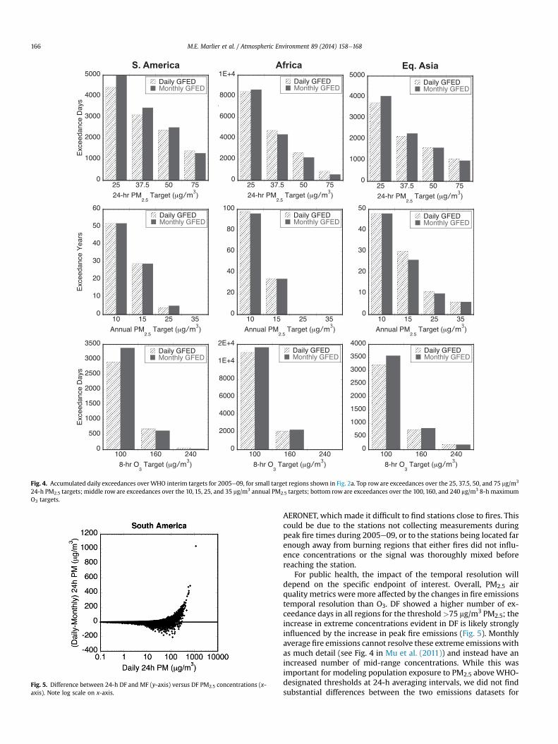
Fig. 4. Accumulated daily exceedances over WHO interim targets for 2005e09, for small target regions shown in Fig. 2a. Top row are exceedances over the 25, 37.5, 50, and 75 mg/m3
24-h PM2.5 targets; middle row are exceedances over the 10, 15, 25, and 35 mg/m3 annual PM2.5 targets; bottom row are exceedances over the 100, 160, and 240 mg/m3 8-h maximumO3 targets.
Fig. 5. Difference between 24-h DF and MF (y-axis) versus DF PM2.5 concentrations (x-axis). Note log scale on x-axis.
M.E. Marlier et al. / Atmospheric Environment 89 (2014) 158e168166
AERONET, which made it difficult to find stations close to fires. Thiscould be due to the stations not collecting measurements duringpeak fire times during 2005e09, or to the stations being located farenough away from burning regions that either fires did not influ-ence concentrations or the signal was thoroughly mixed beforereaching the station.
For public health, the impact of the temporal resolution willdepend on the specific endpoint of interest. Overall, PM2.5 airquality metrics were more affected by the changes in fire emissionstemporal resolution than O3. DF showed a higher number of ex-ceedance days in all regions for the threshold>75 mg/m3 PM2.5; theincrease in extreme concentrations evident in DF is likely stronglyinfluenced by the increase in peak fire emissions (Fig. 5). Monthlyaverage fire emissions cannot resolve these extreme emissionswithas much detail (see Fig. 4 in Mu et al. (2011)) and instead have anincreased number of mid-range concentrations. While this wasimportant for modeling population exposure to PM2.5 above WHO-designated thresholds at 24-h averaging intervals, we did not findsubstantial differences between the two emissions datasets for
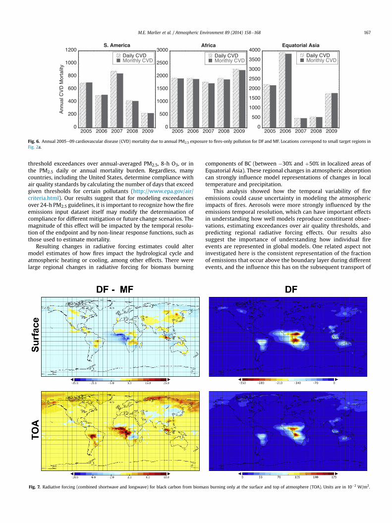
Fig. 6. Annual 2005e09 cardiovascular disease (CVD) mortality due to annual PM2.5 exposure to fires-only pollution for DF and MF. Locations correspond to small target regions inFig. 2a.
M.E. Marlier et al. / Atmospheric Environment 89 (2014) 158e168 167
threshold exceedances over annual-averaged PM2.5, 8-h O3, or inthe PM2.5 daily or annual mortality burden. Regardless, manycountries, including the United States, determine compliance withair quality standards by calculating the number of days that exceedgiven thresholds for certain pollutants (http://www.epa.gov/air/criteria.html). Our results suggest that for modeling exceedancesover 24-h PM2.5 guidelines, it is important to recognize how the fireemissions input dataset itself may modify the determination ofcompliance for different mitigation or future change scenarios. Themagnitude of this effect will be impacted by the temporal resolu-tion of the endpoint and by non-linear response functions, such asthose used to estimate mortality.
Resulting changes in radiative forcing estimates could altermodel estimates of how fires impact the hydrological cycle andatmospheric heating or cooling, among other effects. There werelarge regional changes in radiative forcing for biomass burning
Fig. 7. Radiative forcing (combined shortwave and longwave) for black carbon from bioma
components of BC (between �30% and þ50% in localized areas ofEquatorial Asia). These regional changes in atmospheric absorptioncan strongly influence model representations of changes in localtemperature and precipitation.
This analysis showed how the temporal variability of fireemissions could cause uncertainty in modeling the atmosphericimpacts of fires. Aerosols were more strongly influenced by theemissions temporal resolution, which can have important effectsin understanding how well models reproduce constituent obser-vations, estimating exceedances over air quality thresholds, andpredicting regional radiative forcing effects. Our results alsosuggest the importance of understanding how individual fireevents are represented in global models. One related aspect notinvestigated here is the consistent representation of the fractionof emissions that occur above the boundary layer during differentevents, and the influence this has on the subsequent transport of
ss burning only at the surface and top of atmosphere (TOA). Units are in 10�2 W/m2.
M.E. Marlier et al. / Atmospheric Environment 89 (2014) 158e168168
pollution. In this study, we mixed fire emissions in the boundarylayer, since previous work in Indonesia and North America hasfound that the majority of fire plumes are trapped within stableatmospheric layers (Tosca et al., 2011; Val Martin et al., 2010).However, it would be worth examining the impact of using hightemporal resolution injection heights in future global studies.Also, further investigation will explore the robustness of our re-sults to different atmospheric models with multiple spatial reso-lutions and the sensitivity to using diurnal resolution fireemissions.
Acknowledgments
The authors would like to thank Ruth DeFries for helpful dis-cussions regarding this work. We acknowledge funding supportfrom the NSF Graduate Research Fellowship Program, NASA MAPand ACMAP programs, the NASA High-End Computing (HEC) Pro-gram through the NASA Center for Climate Simulation (NCCS), andNASA grant NNX11AF96G.
Appendix A. Supplementary data
Supplementary data related to this article can be found at http://dx.doi.org/10.1016/j.atmosenv.2014.02.039.
References
Andreae, M.O., Merlet, P., 2001. Emission of trace gases and aerosols from biomassburning. Global Biogeochemical Cycles 15 (4), 955e966.
Atwood, S.A., et al., 2013. Analysis of source regions for smoke events in Singaporefor the 2009 El Niño burning season. Atmospheric Environment 78, 219e230.
Baccini, A., et al., 2012. Estimated carbon dioxide emissions from tropical defores-tation improved by carbon-density maps. Nature Climate Change 2 (3), 182e185.
Boersma, K.F., et al., 2008. Intercomparison of SCIAMACHY and OMI troposphericNO2 columns: observing the diurnal evolution of chemistry and emissions fromspace. Journal of Geophysical Research 113 (D16S26).
Chen, Y., et al., 2009. The sensitivity of CO and aerosol transport to the temporal andvertical distribution of North American boreal fire emissions. AtmosphericChemistry and Physics 9 (17), 6559e6580.
CIESIN, 2005a. Gridded Population of the World Version 3 (GPWv3): PopulationGrids. Socioeconomic Data and Applications Center (SEDAC), Columbia Uni-versity, Palisades, NY. Palisades, NY. Available at: http://sedac.ciesin.columbia.edu/gpw.
CIESIN, 2005b. Gridded Population of the World: Future Estimates, 2015(GPW2015): Population Grids. Socioeconomic Data and Applications Center(SEDAC), Columbia University, Palisades, NY. Palisades, NY. Available at: http://sedac.ciesin.columbia.edu/gpw.
Duncan, B.N., et al., 2003. Interannual and seasonal variability of biomass burningemissions constrained by satellite observations. Journal of GeophysicalResearch 108 (D2), 4100.
Giglio, L., et al., 2009. An active-fire based burned area mapping algorithm for theMODIS sensor. Remote Sensing of Environment 113 (2), 408e420.
Giglio, L., et al., 2010. Assessing variability and long-term trends in burned area bymerging multiple satellite fire products. Biogeosciences 7, 1171e1186.
Guenther, A., et al., 1995. A global model of natural volatile organic compoundemissions. Journal of Geophysical Research 100 (D5), 8873e8892.
Guenther, A., et al., 2006. Estimates of global terrestrial isoprene emissions usingMEGAN (Model of Emissions of Gases and Aerosols from Nature). AtmosphericChemistry and Physics 6, 3181e3210.
Heald, C.L., et al., 2003. Biomass burning emission inventory with daily resolution:application to aircraft observations of Asian outflow. Journal of GeophysicalResearch 108 (D21), 8811.
Holben, B., et al., 1998. AERONETdA federated instrument network and data archivefor aerosol characterization. Remote Sensing of Environment 66 (1), 1e16.
Kaiser, J.W., et al., 2012. Biomass burning emissions estimated with a global fireassimilation system based on observed fire radiative power. Biogeosciences 9(1), 527e554.
Koch, D., Schmidt, G.A., Field, C.V., 2006. Sulfur, sea salt, and radionuclide aerosolsin GISS ModelE. Journal of Geophysical Research 111 (D06206).
Lamarque, J.-F., et al., 2010. Historical (1850e2000) gridded anthropogenic andbiomass burning emissions of reactive gases and aerosols: methodology andapplication. Atmospheric Chemistry and Physics 10 (15), 7017e7039.
Langmann, B., et al., 2009. Vegetation fire emissions and their impact on airpollution and climate. Atmospheric Environment 43, 107e116.
Lee, Y.H., et al., 2013. Evaluation of preindustrial to present-day black carbon and itsalbedo forcing from Atmospheric Chemistry and Climate Model Intercompar-ison Project (ACCMIP). Atmospheric Chemistry and Physics 13 (5), 2607e2634.
Mu, M., et al., 2011. Daily and hourly variability in global fire emissions and con-sequences for atmospheric model predictions of carbon monoxide. Journal ofGeophysical Research 116 (D24303).
Ostro, B., 2004. Outdoor Air Pollution: Assessing the Environmental Burden ofDisease at National and Local Levels. World Health Organization, Geneva.
Pope, C.A., et al., 2011. Lung cancer and cardiovascular disease mortalityassociated with ambient air pollution and cigarette smoke: shape of theexposure-response relationships. Environmental Health Perspectives 119,1616e1621.
Price, C., Penner, J., Prather, M., 1997. NOx from lightning 1. Global distribution basedon lightning physics. Journal of Geophysical Research 102 (D5), 5929e5941.
Rayner, N.A., et al., 2003. Global analyses of sea surface temperature, sea ice, andnight marine air temperature since the late nineteenth century. Journal ofGeophysical Research 108 (D14), 4407.
Reid, J.S., et al., 2009. Global monitoring and forecasting of biomass-burning smoke:description of and lessons from the fire locating and modeling of burningemissions (FLAMBE) program. IEEE Journal of Selected Topics in Applied EarthObservations and Remote Sensing 2 (3), 144e162.
Rienecker, M.M., et al., 2011. MERRA: NASA’s modern-era retrospective analysis forresearch and applications. Journal of Climate 24, 3624e3648.
Shindell, D.T., et al., 2013a. Radiative forcing in the ACCMIP historical and futureclimate simulations. Atmospheric Chemistry and Physics 13 (6), 2939e2974.
Shindell, D.T., et al., 2013b. Interactive ozone and methane chemistry in GISS-E2historical and future climate simulations. Atmospheric Chemistry and Physics13 (5), 2653e2689.
Tosca, M.G., et al., 2011. Dynamics of fire plumes and smoke clouds associated withpeat and deforestation fires in Indonesia. Journal of Geophysical Research 116(D08207).
UN, 2011. World Population Prospects: the 2010 Revision, CD-ROM ed. Departmentof Economic and Social Affairs Population Division.
Val Martin, M., et al., 2010. Smoke injection heights from fires in North America:analysis of 5 years of satellite observations. Atmospheric Chemistry and Physics10, 1491e1510.
van der Werf, G.R., et al., 2008. Climate regulation of fire emissions and defores-tation in equatorial Asia. Proceedings of the National Academy of Sciences 105,20350e20355.
van der Werf, G.R., et al., 2010. Global fire emissions and the contribution ofdeforestation, savanna, forest, agricultural, and peat fires (1997e2009). Atmo-spheric Chemistry and Physics 10 (23), 11707e11735.
Voulgarakis, A., et al., 2011. Global multi-year O3eCO correlation patterns frommodels and TES satellite observations. Atmospheric Chemistry and Physics 11(12), 5819e5838.
Voulgarakis, A., et al., 2013a. Analysis of present day and future OH and methanelifetime in the ACCMIP simulations. Atmospheric Chemistry and Physics 13,2563e2587.
Voulgarakis, A., Shindell, D.T., Faluvegi, G., 2013b. Linkages between ozone-depleting substances, tropospheric oxidation and aerosols. AtmosphericChemistry and Physics 13 (9), 4907e4916.
Wang, J., Christopher, S.A., 2006. Mesoscale modeling of Central American smoketransport to the United States: 2. Smoke radiative impact on regional surfaceenergy budget and boundary layer evolution. Journal of Geophysical Research111 (D14S92).
Wiedinmyer, C., et al., 2011. The Fire INventory from NCAR (FINN): a high resolutionglobal model to estimate the emissions from open burning. Geoscientific ModelDevelopment 4 (3), 625e641.
World Health Organization, 2006. WHO Air Quality Guidelines for ParticulateMatter, Ozone, Nitrogen Dioxide and Sulfur Dioxide. World Health Organiza-tion, Geneva.
World Health Organization, Department of Measurement and Health Information(WHO), 2011. Death Estimates for 2008 by Cause for WHO Member States.Available at: http://www.who.int/healthinfo/global_burden_disease/estimates_country/en/index.html.
Wu, L., Su, H., Jiang, J.H., 2011. Regional simulations of deep convection and biomassburning over South America: 2. Biomass burning aerosol effects on clouds andprecipitation. Journal of Geophysical Research 116 (D17).