The segmented marriage market

The influence of geographical homogamy on marital mobility in 19th

century Belgian cities

Bart Van de Putte

bart.vandeputte@soc.kuleuven.be

Postdoctoral Fellow of the Fund for Scientific Research – Flanders (Belgium)

Centre for Population and Family Research

Department of Sociology

Catholic University of Leuven

Van Evenstraat 2B

B-3000 Leuven

Belgium

fax number: +32 16 32 33 65

Paper prepared for the IEHC 2006

XIV International Economic History Congress

Helsinki, Finland, 21 to 25 August 2006

SESSION 34: Migration, Family and Economy in Industrializing and Urbanizing

Communities

1

Introduction Migration has often been linked to marital mobility according to social origin (see amongst many, Bras 1998, Schrover 2004, Sewell 1976, Dribe et al. 2005, Van de Putte et al. 2005). Several causes were identified. Migrants, it is believed, escaped the parental or local web of social control, and this facilitated a heterogamous marriage in terms of social origin – further called social heterogamy (Sewell 1976, see also Oris et al. 2002). Sometimes migrants were pushed to leave their home region just as a consequence of (potential) downward social mobility, what always has consequences for marital mobility (Van de Putte et al. 2005). Migrants are also sometimes considered to be a selected group of dynamic people travelling to new destinations to realise upward intergenerational social mobility (see Dribe et al. 2005, Bras 1998), for example to become merchant, civil servant or domestic servant in the city, or even to explore the marriage market and to find a good marriage partner (Dribe et al. 2005). In spite of much research, there does not really appear clear and systematic evidence for a specific relation between migration and marital mobility (see for example Van de Putte 2005, Bras & Kok 2005). To unravel this relation we might have to examine other features of the partner selection pattern of migrants. There are, for example, many studies that provide evidence for homogamy by migration status – further called geographical homogamy (Klesman 1987, King 1997, Jacquemin 1998, Shanahan & Olzak 1999, Oris 2000, Van de Putte 2003). Both practical barriers and mutual prejudices are seen as the causes of this phenomenon. The existence of geographical homogamy implies that the marriage market is segmented. Natives and migrants search marriage partners on different marriage markets, it seems, instead of on one big market. In our view, this will inevitably have consequences for the relation between migration and marital mobility. A good point of departure to tackle this problem is provided by three specific theses developed in sociological research on the relation between geographical origin and social homogamy in 20th century societies. First, there is the byproduct-effect, that claims that homogamy according to one characteristic (e.g. social homogamy) is the automatic result of homogamy according to another characteristic (e.g. geographical homogamy), in case these characteristics are correlated. In this way, the segmentation of the marriage market by migration status can result in social homogamy. Second, there is the Blau-thesis on the effect of cross-sectional cleavages. Blau et al. (1984) state that in societies where social cleavages (e.g. by social origin and migration status) are not correlated, marriage candidates will marry a partner with a characteristic that reflects their priority affiliation (e.g. native status) and are therefore more or less forced to accept heterogamy on other characteristics (e.g. social origin). Under these conditions, the segmentation of the marriage market by migration status makes it difficult to marry homogamous. A third thesis is the so-called exchange-effect. This thesis states that a migrant background – typically evaluated negatively – is often compensated by a higher social position. In other words, migrants who cross the boundaries of the segmented marriage market by marrying a native partner will have to pay the price of integration by accepting (downward) social heterogamy. As we know that particularly rural migrants are often isolated on the marriage market, these theses might be valid for some 19th century cities as well. To test this, we examine partner selection in three 19th century Belgian cities, Leuven, Aalst and Gent, using marriage certificates. In this paper we aim to provide some methodological tools to study the effect of the segmentation of the marriage market and hope to show that it indeed influences patterns of social homogamy.

2

1. Theory Migration status is often a basis for group formation. Cultural differences, prejudices and discrimination may lead to the avoidance of 'the other' in all kinds of social interactions (in marriage, leisure, etc.). Migration may also lead to spatial segregation, defined as the concentration of migrants in one or more neighbourhoods. Both avoidance and segregation lead to the emergence of separate, segmented marriage markets. As a consequence, partner selection according to social origin can be influenced. There are three specific theses that help to clarify this. First, the social structure (broadly defined as a population's distribution among social positions along various lines, e.g. social origin, geographical origin; see Blau et al. 1984) may impose a specific marriage pattern. In some cases, geographical and social origin are correlated. This may, for example, be the result of a specific type of migration (e.g. due to a high number of unskilled workers among migrants) although it might also be the consequence of systematic discrimination. As a result, migrants may be over-represented among specific social groups (e.g. the unskilled, the farmers) and under-represented in others (e.g. among skilled workers). If this difference in social structure between natives and migrants is combined with geographical homogamy, social homogamy will be the automatic result (byproduct-effect, see Uunk 1996 in particular, also Kalmijn 1998 and Van de Putte 2005).1 The logic of this effect is fairly straightforward. Because of geographical homogamy, there are, in practice, segmented marriage markets (of natives and migrants). Given the fact that the social structure (here narrowly understood as the distribution of individuals by social origin) always determines the pattern of partner selection (the social structure can be seen as the 'opportunity' structure: the chance to marry a person with a particular characteristic based on the presence of that characteristic in a given society), it is important that the social structure differs between these segments. In the migrant segment, for example, some categories will be over-represented. And as most migrants marry migrants, they will typically have more chance to marry a partner that belongs to this over-represented category. If, for example, almost all migrants are children of farmers, they have a fair chance to marry a farmer's child in case their partner selection is restricted to the migrant marriage market. Consequently, the overall social structure (typically used to measure the opportunity structure) becomes an incorrect basis for the estimation of the opportunity structure in a segmented marriage market. Therefore, levels of social homogamy will be biased. This bias will be particularly strong when migration is very selective. The presence of one or more large classes on the migrant marriage market will result in high levels of social homogamy among migrants.2 Related to the byproduct-thesis is the Blau-thesis that states that intersecting social affiliations stimulate intermarriage (Blau et al. 1984). Intersection signifies that people belong to different groups (e.g. one is migrant, middle class, old, …) and meet different people in these different groups. For example, the native elite meets both natives (among whom middle and lower class natives) and elite people (among whom migrants and natives). Blau et al.

1 The existence of a triple melting pot in the United States can be explained in this way. The marriage market was composed of three segments, defined by religion. As religion was an important criterion in partner selection, it led to a specific pattern of partner selection according to nationality. For example, Polish, Italian and Irish Catholics married among each other (Kennedy 1944). 2 Migrants are of course not always a minority with a specific social profile, see for example the situation in cities born by industrialisation, such as Tilleur, where almost all city inhabitants are migrants (Van de Putte et al. 2005).

3

claim that in societies where people have different and intersecting positions, marriage candidates select a characteristic (e.g. native) to which they give priority. It is this priority preference that will be applied in the screening of potential partners. They will of course have many more preferences (e.g. they might also want to marry an elite partner). Yet, in case there is no association between the two characteristics (e.g. not all natives are elite) it might become quite difficult to combine all preferences. Consequently, intermarriage according to the other characteristics is stimulated. In other words, if people choose their migrant status as the priority, geographically unmixed couples will have to accept higher levels of social heterogamy. A specific example of this Blau-effect can be found in the effect of pillarisation (defined as the existence of clusters of organisations based on ideological principles, such as denomination or political ideology) on partner selection. Pillars typically unite persons from different social classes. In case these pillars also function as a marriage market – the 'pillar' is the priority preference – the result is automatically social heterogamy (see Beekink et al. 1998, Bras & Kok 2005: 253). This Blau-thesis refers to different conditions than the byproduct-effect. In the former, there is no association between social and geographical origin, while in the latter there is an association. Consequently, whether in a given society one of these theses apply, depends on the relation between social and geographical origin. The Blau-effect is however more than the complementary effect of the byproduct-effect. It is probable that finding a partner that also meets a second criterion is more difficult than can be assumed given a specific opportunity structure. The size of the one's group may play a role. The smaller the size, the more difficult it is to find a partner that meets all criteria (see also Schrover 2004). In that case it is less easy to combine both social and geographical origin – search costs increase – and consequently the Blau-thesis seems to be applicable. Above we stated that in our view the byproduct-effect will typically apply for unmixed migrant couples. For the native couples, the Blau-thesis is perhaps more likely. For the native group social differentiation is typically stronger. Furthermore, natives are probably more likely to choose geographical origin as the priority preference. An example of this is the hostile reaction of the native French-speaking Liège inhabitants towards the rural, Dutch-speaking Flemish migrants (Van de Putte et al. 2005). For (male) migrants, on the contrary, it is typically very useful to marry a native in order to enhance their integration (see Alter 1988 on Verviers), but of course, they can only do so if they are allowed to by the native citizens. Third, there is the exchange or Davis-Merton thesis that claims that a low status migrant background needs to be compensated by a higher social origin/position (for a discussion, see Kalmijn 1998). The exchange-thesis starts from the idea that the marriage partner selection is a bargaining process. From this view, one can only marry upward in case other advantages are proposed. In this way, upward marital mobility can be 'bought' by one's native status. From the migrant's perspective, the bargaining process forces him or her to accept downward mobility to compensate for the inferior migrant status. For example, Afro-Americans can marry White Americans, but typically with the cost of having to marry downward. Given the prejudices towards migrants born on the countryside, we expect this effect to be present in 19th century cities (see further). For migrants, entering the native marriage market implies having to pay the price of integration by downward marriage.

4

The consequence of this exchange-effect is a higher level of social heterogamy among the geographically mixed couples, and, in particular a higher level of downward heterogamy for migrants marrying natives (note: we will further use 'mixed' and 'unmixed' to refer to geographical homogamy). In this way, the exchange-effect reinforces the byproduct-effect. The byproduct-effect leads to social heterogamy among the mixed because of structural conditions. The exchange-effect adds to this that entering the other segment of the marriage market gives you weaker (for migrants) or stronger (for natives) bargaining position. Mind however that the exchange-effect should be present regardless of the structural conditions imposed by differences in the native and migrant social structure. Even when for a geographically mixed couple a homogamous marriage is possible, this is not likely to happen in case exchange-logics are applied. Based on this discussion, we derive the following propositions:

- migrants who are avoided by natives and who have a different social structure, will have high levels of social homogamy because of the byproduct-effect

- migrants who belong to an avoided group, will have high levels of social heterogamy in case they do marry with natives, because of the exchange-effect

- migrants and (particularly) natives who see geographical origin as their priority criterion, will have a higher level of social heterogamy as it is difficult to combine their priority preference with other criteria (Blau-effect). This will be particularly the case for those who belong to small groups.

We continue this paper with a description of the sources (section 2.1). In section 2.2 we discuss the methodology, in which we spend most of our attention to the construction of variables measuring different aspects of the marriage market. Next, we will give a short description of the cities in section 2.3, in which we discuss to what extent the conditions in these cities are favourable for one of the described effects. 2. Data, context, methodology 2.1. Data We use marriage certificates from Civil Registration registers (1800-1913). The certificates contain information on the marriage itself, some demographic history of the spouses (and their parents), their occupation, their place of residence, place of birth, etc. Marriage certificates are available for the entire period. Different sampling strategies have been used: for Gent, one in twelve marriage certificates were included; for Leuven and Aalst one in three marriage certificates. These marriage certificates permit to measure most variables relevant to this study. The first important variable is social origin, defined as the social position of the father of the spouses. To classify individuals according to their social origin, we apply the SOCPO-scheme to the occupational titles in the marriage certificates. This scheme is presented in detail in Van de Putte & Miles (2005).3 This classification distinguishes between five 'social power’ (or SP) 3 The SOCPO-scheme codes the HISCO-codes (van Leeuwen et al., 2002). HISCO is a functional classification distinguishing between occupations on the basis of the tasks associated with the occupations. Each occupational group gets a five-digit code (e.g. 75400 for ‘weaver’). Other information, e.g. on employment status, is stored in separate codes. A list of hiscodes coded into SOCPO can be found in Van de Putte & Miles, 2005.

5

levels using skill, possession, position within a hierarchical organisational structure and prestige characteristics as criteria. Lower class subgroups are: SP-level 1 (mainly unskilled workers), SP-level 2 (mainly semi-skilled workers) and SP-level 3 (mainly skilled workers). The middle class (SP-level 4) is mainly composed by master artisans, retailers, farmers, clerks etc. SP-level 5 (the ‘elite’) comprises white collar/professional specialists (e.g. lawyers), wholesale dealers, factory owners, etc. The second important variable is migration status. We use the place of birth recorded in the marriage certificate to classify individuals. We distinguish between natives (born in the place of marriage) and migrants (born elsewhere). In the latter category we make a further subdivision between rural and non-rural migrants. Previous studies confirm the importance of this cleavage, particularly in terms of cultural dissimilarity, with rural migrants being the ones least adapted to urban culture (for an overview, see Van de Putte 2003). This dissimilarity is indicated by mutual prejudices. We use the number of inhabitants in the place of birth as the criterion to distinguish both migrant groups. Individuals born in a place that counted less than 4000 inhabitants in 1900, are categorised as rural, the others as non-rural. Villages with less than 4000 inhabitants were small during the whole 19th century. Previous research shows that this criterion is useful, that is, we found significant differences between both categories, in terms of partner selection and other criteria (Van de Putte 2003, Van de Putte 2005). It is evident that much detail in the migration history of individuals is lost when using marriage certificates, such as the time of entrance in the city, the family context of migration, etc. The use of marriage certificates to study the marriage market is not unproblematic. A key issue is how to define the population at risk (of getting married). This risk population needs to be defined, as it is the basis on which the opportunity structure is calculated. In research on marital mobility, the opportunity structure is typically estimated by the social structure. By using marriage certificates we assume that the social structure (and therefore also the opportunity structure) of those who marry does not differ from the social structure of those who are on the marriage market. This is not necessarily correct, yet, this source does permit to study segregation processes occurring on the marriage market. The main consequence of the potential bias is that we might ignore exclusion processes that do only lead to the exclusion of some categories from the marriage market. For example, if rural migrants or unskilled workers are avoided, this may limit their access to marriage. This exclusion will not be observed as it does not lead to high levels of homogamy among the rural migrants or the unskilled. However, as exclusion is often directed to both males as females, the excluded have the possibility to marry each other, and therefore we will measure the exclusion of most groups (for an extensive discussion, see Van de Putte 2005). 2.2. Methodology The central aim of the empirical analysis is to show that the propositions formulated above are useful to understand differences in the level of social homogamy between migrants and natives. In order to do so, we construct a series of logistic regression models. We start from a basic model without taken the segmentation of the marriage market into account. Stepwise we add independent variables to examine the role of segmentation. Table 1 might be helpful to understand our approach and our worries. Before we present the models and variables, we first address some general methodological topics. The segmentation of the marriage market may influence social homogamy in two

6

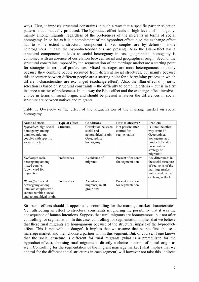
ways. First, it imposes structural constraints in such a way that a specific partner selection pattern is automatically produced. The byproduct-effect leads to high levels of homogamy, mainly among migrants, regardless of the preferences of the migrants in terms of social homogamy. In so far as it is a complement of the byproduct-effect, also the exchange-effect has to some extent a structural component (mixed couples are by definition more heterogamous in case the byproduct-conditions are present). Also the Blau-effect has a structural component: it leads to social heterogamy in case geographical homogamy is combined with an absence of correlation between social and geographical origin. Second, the structural constraints imposed by the segmentation of the marriage market are a starting point for strategies in terms of preferences. Mixed marriages are more heterogamous, not only because they combine people recruited from different social structures, but mainly because this encounter between different people are a starting point for a bargaining process in which different characteristics are exchanged (exchange-effect). Also, the Blau-effect of priority selection is based on structural constraints – the difficulty to combine criteria – but is in first instance a matter of preferences. In this way the Blau-effect and the exchange-effect involve a choice in terms of social origin, and should be present whatever the differences in social structure are between natives and migrants. Table 1. Overview of the effect of the segmentation of the marriage market on social homogamy Name of effect Type of effect Conditions How to observe? Problem Byproduct: high social homogamy among unmixed migrant couples with specific social structure

Structural Correlation between social and geographical origin Geographical homogamy

Not present after control for segmentation

Is it not the other way around? Geographical homogamy as a product of status preservation strategy of migrants?

Exchange: social heterogamy among mixed couples (downward for migrants)

Preferences Avoidance of migrants

Present after control for segmentation

Are differences in the social structure of segments of the marriage market not caused by the exchange-effect?

Blau-effect: social heterogamy among unmixed couples who cannot combine social and geographical origin

Preferences Avoidance of migrants, small group size

Present after control for segmentation

Structural effects should disappear after controlling for the marriage market characteristics. Yet, attributing an effect to structural constraints is ignoring the possibility that it was the consequence of human intentions. Suppose that rural migrants are homogamous, but not after controlling for segmentation. In this case, controlling for segmentation implies that we believe that these rural migrants are homogamous because of the structural impact of the byproduct-effect. This is not without 'danger'. It implies that we assume that people first choose a marriage market, and then choose a partner within this segment. But, of course, if one knows that the social structure is different for rural migrants (what is a prerequisite for the byproduct-effect), choosing rural migrants is directly a choice in terms of social origin as well. Controlling for the segmentation of the migrant marriage market (what implies that we control for the different social structures in each segment) will however not take this 'indirect'

7

choice into calculation. Not controlling for the byproduct-effect, on the other hand, would mean that we think that these rural migrants are homogamous because they have a strong preference for partners with a similar social origin. Not controlling for segmentation implies that we see individuals as agents with free will and with the possibility to overcome any structural constraint. This seems quite unrealistic, yet, also the opposite view ('humans have hardly any free will') is of course also unrealistic. Preference-effects should be present after controlling for the marriage market, as they do not (entirely) depend on the specificity of the social structure. Controlling for the segmentation of the marriage market implies that we believe that segmentation is that strong that people have to undergo its impact completely. Controlling for segmentation therefore poses rigid tests for any preference related effect (e.g. the exchange-effect) that might have similar empirical consequences as structural constraints have. Indeed, characteristics of the marriage market (different social structures in each segment) might be the consequence of a preference-related strategy. Controlling for it, excludes this, and this might be incorrect. In the empirical analysis we will compare the results of variant models (each controlling, or not, for specific structural constraints) and reflect on the underlying assumptions. But ultimately, the question will remain the same: in how far is an individual's behaviour determined by structure, and to what extent is it possible for an individual to overcome these structural constraints? Regardless of this 'philosophical problem', there is the more technical problem that we have to devise specific ways to control for the segmentation of the marriage market. In other words, we have to think of variant ways in which the marriage market structures the behaviour of the marriage candidates. We will construct several variables that aim to account for the segmentation of the marriage market. The procedure presented in the section below does not offer a rigid method. Each variant model is based on assumptions, and it remains a complicated task to interpret the results. Model 1: the basic model We start with a description of the basic model. We choose social heterogamy (1)/social homogamy (0) as the categorisation of the dependent variable. We take the perspective of the groom and examine whether his migration status can explain his chance to marry homogamous. Taking the perspectives of one of the spouses is a didactical trick that allows a straightforward interpretation of the partner selection pattern.4 In the basic model we use migration status groom, group size, period, social origin groom, intergenerational mobility groom and age as the independent variables (model 1). The estimates of this model show what the effect is of being a migrant, controlled for some standard and classic control variables. The reason to include period and social origin groom is straightforward. We shortly discuss the other variables (see the appendix for the categorisation of all variables).

4 Also the perspective of the brides can be taken. Usually, there will not be differences, as the group sizes are typically the same for grooms and brides of the same level. We did the analysis from the other perspective, but this did not show substantial differences.

8

The group size variable is of special importance. By this variable we measure the chance to marry a partner who has the same social origin. It therefore controls for the impact of the social structure on the chance to marry homogamous. In model 1 we use an unsegmented group size variable. We assume that there are no segments on the marriage market, and therefore, we assume that natives and migrants have the same chance to marry homogamous, taking however their own social origin and the period in which they married into account. The variable is calculated in this way: for groom x belonging to SP-level y in Period z the group size value is equal to the percentage of brides in SP-level y in Period z. The interpretation is straightforward: the higher the score for this group size variable, the lower the chance to marry heterogamous (for more information see Van de Putte 2005, for a similar approach, see: Wildsmith et al. s.d., Bras & Kok, 2005). We include age to control for the timing of the entrance on the marriage market, typically related to migration (Oris 2000, and in general Kasakoff & Adams 1995). Whatever the reason of the late entrance of migrants, for example the difficulty to find a partner or the late arrival in the city, this may seriously influence their partner selection. It leads to higher chance to marry other migrants (in case age homogamy is present, what is often the case, Van de Putte 2005), and is therefore another source of the segmentation of the marriage market. As migration may be related to intergenerational social mobility, we also include this variable into the model. This relation may be both direct (e.g. people migrate because of a wish to climb on the social ladder) and indirect (the migrant social structure may differ from the native social structure, and social classes typically differ in their levels of intergenerational mobility). And as we know that, even in societies that are not particularly meritocratic, intergenerational social mobility is a strong determinant of social heterogamy, this may be another way in which migration affects partner selection according to social origin. Model 2: controlling for the structural constraints induced by the segmentation of the marriage market by geographical origin Model 1 shows what we would observe if we ignore the considerations discussed above. In model 2 we replace the dichotomous migration status variable by a trichotomous one, separating rural from non-rural migrants. This model aims to show whether such a distinction is necessary to have a precise insight in the influence of migration on marital mobility. We use four different variants of model 2, each of which includes a different group size variable. Model 2A includes the unsegmented group size variable. To use the unsegmented group size variable implies that we assume that are no boundaries on the marriage market. Or in other words, that we think that individuals never choose a partner based on geographical origin as a first criterion. Given the numerous accounts of geographical homogamy, this is not realistic. Therefore, in case there is some segmentation, these group sizes are not correct. In case conditions are favourable for a byproduct-effect, homogamy of those on the segmented marriage market will be overestimated, as part of it is simply the product of the specificity of the social structure in their segment of the marriage market. In model 2B we replace the unsegmented group size variable by a segmented group size variable. By this replacement we assume that natives, rural and non-rural migrants operate on different marriage markets. On a segmented marriage market, the availability of brides belonging to the same category as the groom is the percentage of that category among the

9

brides with the same geographical origin. The segmented group size variable is calculated as follows: for native groom x belonging to SP-level y in Period z the group size value is equal to the percentage of brides in SP-level y in Period z among the natives; for migrant groom x belonging to SP-level y in Period z the group size value is equal to the percentage of brides in SP-level y in Period z among the migrants. If there is not much difference between using the one rather than the other variable, this may indicate that marriage markets are not segmented or are not very different in terms of their social structure. Yet, both the unsegmented as the segmented group sizes are based on a rigid, and incorrect assumption. Both refer to an extreme situation: no segmentation versus perfect segmentation. In practice there are always people, in any society, who do not use geographical origin as a first criterion. These people are not limited to 'their' segment of the marriage market. For those who are not part of the segmented marriage market, the group sizes are biased. An alternative measure could be to use the observed marriage market to calculate group sizes. If, for example, a groom, migrant or native, marries a native person, this groom is apparently present on the native marriage market, and then the opportunity structure can be calculated using the native marriage market as the starting point. For Model 2C we use this observed group size variable (see appendix for calculation details). Also this method has some disadvantages. Even the observation of marrying a native partner does not necessarily imply that the groom was only present on the native marriage market. The groom might, perhaps, as well have married a migrant bride. For those who marry a dissimilar partner, one could argue, the best estimation of the group sizes are based on the characteristics of the whole marriage market. We therefore propose a final variant that includes a different type of observed group sizes variable (observed group sizes_2, used in model 2D). To calculate this variant variable we assume that those with a mixed marriage were operating on an unsegmented marriage market, instead of on the native or migrant market. For people who marry a person similar according to geographical origin we still assume a segmented marriage market.5 Model 3: Differences in social homogamy between mixed and unmixed couples In model 3A, B, C and D we replace the migration status variable by a 'composition by geographical origin'-variable. By using this variable, we compare levels of social heterogamy between couples defined by their geographical composition. Model 3 allows to test whether there is an exchange-effect. In that case mixed couples, especially when one of the partners has a rural background, will show higher levels of heterogamy. It also allows to test whether there is a Blau-effect. In that case, unmixed couples, in particular native unmixed couples, will show higher levels of social heterogamy. We examine four variants of model 3. In model 3A we use the regular unsegmented group size, in model 3B the segmented group sizes, in model 3C and D we use observed group sizes. Model 3C is the most strict variant, but has some practical advantages. The use of observed group sizes implies that those who married a native bride get the group sizes of the native marriage market, and that those who marry migrants get the group sizes of the migrant 5 Perhaps also other models could be useful, e.g. assuming three segments: native, migrant and mixed marriage market, from which we excluded the unmixed when calculating group sizes.

10

marriage market. This definition of group sizes is especially important when a variable that measures the composition of the couple by migration status is included in the model. Including this variable creates some interpretational problems. As soon as there is an association between social and geographical origin, mixed and unmixed couples will show different levels of social homogamy, even if there is no form of segregation or avoidance (or geographical homogamy). If, for example, migrants are over-represented among the unskilled, persons who marry a migrant will have more chance of marrying an unskilled. Consequently, differences in social homogamy between the mixed and unmixed do not necessarily prove that avoidance has an impact on social homogamy patterns. It is just the reflection of the association between social and geographical origin. Ignoring this would weaken the test of the Blau- and exchange-effect. Controlling for the group sizes found in every niche of the marriage market, excludes this confusion. By using model 3C, we have a strict, but conservative test. But, as stated above, using model 3C also makes it impossible to see the choice for a specific niche of the marriage market as an act of showing a preference for a specific type of marriage. To sum up, all these models are based on assumptions. Where necessary, we will discuss these issues in some more detail in the empirical analysis. Perhaps the best strategy is a conservative one: effects are only present when measured by all variants. 2.3. Context: migration and partner selection in Leuven, Aalst and Gent Gent was a historical and big city. Its economy was mainly based on the cotton sector, but also other branches of the textile sector and engineering were important. Gent experienced a spectacular ‘take off' in the early 19th century, based on its cotton industry (Mokyr 1976: 27). In the first half of the 19th century the combination of economic transformation, population growth (from 50.000 to 100.000 in the first half of the 19th century), migration and decreasing standard of living create living conditions that are best described as an urban crisis. In the second half of the 19th century the economic transition and population growth slowed, while the standard of living rose gradually. The textile industry remained the dominant sector during the 19th century. Large industrial concentrations were also present in Aalst, although industrialisation developed only late in the 19th century. Before 1880-1890 factories were still small (less than 100 workers) and many workers were employed in the agricultural sector of this small city (about 12.000 inhabitants in 1800, about 18.000 in 1850). After 1880-90 the textile industry was expansive and factories became larger. Also in Aalst, the period of industrialisation was accompanied by strong population growth (30.000 inhabitants in 1900) and a phase of low standard of living. Leuven was originally a middle-sized town, with about 20.000 inhabitants in 1800. In the 19th century Leuven industrialisation was not very pronounced. But also the Leuven economy lost it traditional (artisanal and agricultural) roots. This change was however gradual and did not result in many large-scale enterprises. Leuven also played an important role in administration and education. By 1900 the city counted about 42.000 inhabitants. There are quite some differences in the migration history of the three cities (figures in this section based on Van de Putte 2005). First, there is the size of the migrant group. In Aalst, the proportion of grooms (first marriages) not born in the city fluctuated between 25 and 35% in

11

the period 1800-1913. This proportion of migrant grooms was higher in Leuven (between 35 and 45%) and Gent (between 39 and 48%). For brides, the differences were similar, but the proportion of migrants was somewhat smaller – a consequence of the habit to celebrate the marriage in the place of residence of the bride. Also the composition of the migrant group is different. In Gent, one third of the migrant males was born in a rural area, while this proportion was higher in Leuven (about 50%) and Aalst (54%). These figures relate to the socio-economic characteristics of the cities. As a large economic and administrative center, Gent attracted a larger variety of immigrants, for example to staff the state institutions and private administrations. These immigrants were more likely to come from urban and semi-urban areas. The recruitment was less diverse in Leuven and in particular in Aalst. At the same time, long distance migration was largest in Gent (about 18,7% of the grooms and 16,8% of the brides was born further than 10 km away from the city). In Leuven (13,9 and 10,8 %) and Aalst (6,9 and 5,1%) these percentages were lower. Finally, in the three cities we observed geographical homogamy (Van de Putte 2003). The level of homogamy was highest in Gent and Leuven. In both cities rural migrants in particular had the highest level of homogamy.6 This indicates that they really were the least preferred group in these cities. The homogamy parameter was lower for non-rural migrants. As a consequence, rural migrants had less chance to marry natives in comparison to natives themselves. Also non-rural migrants had less chance to marry natives, but they had more chance in comparison to the rural migrants. Geographical homogamy was less strong in Aalst, in particular in the first half of the 19th century. The latter observation is not unexpected, given the rural character of Aalst. Migrants were not really seen as different from the city inhabitants. These patterns of geographical homogamy were very consistent over time. The social structure was different for natives, rural and non-rural migrants. The association was strongest in Leuven, indicating that the differences in social structure were (somewhat) stronger than in the other cities (for grooms Cramers' V is about 0,23; while 0,17 for Gent and 0,13 for Aalst; for brides Cramers' V is 0,26; while 0,19 for Gent and 0,20 for Aalst). Especially in Leuven, the structure of the rural migrants was skewed. Most of rural migrants (about 60%), were sons of middle class parents, among which farmers. In Aalst (50%) and Gent (45%) this percentages were somewhat lower, what reflects that the social structure was less differentiated. For non-rural migrants, the elite and the middle class was over-represented. This was the case in the three cities. All this leads to the conclusion that the conditions for a byproduct-effect are in particular favourable for rural migrants in Leuven: they have a high level of homogamy, they have an outspoken different and uneven social structure and count for a large proportion of the city population. In Gent, their proportion is smaller, and also their socio-economic profile is somewhat less different. The situation in these cities is very different from the one observed in Aalst, basically because in that city rural migrants are not evaluated as very different from the other city inhabitants. The same is true for the exchange-effect. Especially in Gent and Leuven, rural migrants are most vulnerable for it. As the social structure of natives is quite even, and given the fact that we expect them to have a priority for native marriage partners, conditions are to some extent present for a Blau-effect in Leuven and Gent. Yet, in both these 6 Relative homogamy parameters in saturated log-linear models were about 1.6, what indicates that the association between groom's and brides's geographical origin increased the cell frequency with factor 1.6 (Van de Putte 2003).

12

cities natives are a large group, what probably made it possible to use both social and geographical origin as criteria. Furthermore, especially in Gent, non-rural migrants were a quite large alternative pool of potential marriage partners. 3. Results We start with the analysis of Leuven (table 2). The results of the basic model show no effect for migration status on social heterogamy (model 1). In model 2A we distinguish between rural and non-rural migrants. This reveals that rural migrant grooms have more chance to marry homogamous than native grooms. Non-rural grooms, on the contrary, have more chance to attract a partner from a different class than native grooms. As the results appear in a model that controls for age, intergenerational social mobility and social origin, this difference is related to differences between rural and non-rural migrants that cannot be reduced to these variables. In model 2B we use group sizes that are calculated under the assumption of a segmented marriage market. This is of importance. We do no longer observe significant differences by migration status. Rural migrants are clearly no more homogamous than can be expected given the situation in their niche of the marriage market, while the estimate for non-rural migrants does remain higher than 1 (although not significant). In model 2C and 2D we use observed group sizes. The estimates for rural migrants are, again, lower. Mind that only for model 2C the estimates are significant. The question is, then, what assumption is most valid for Leuven. The choice makes a difference. Chosing for model 2A or C implies that we find significant levels of homogamy among rural migrants – we attribute the level of homogamy to characteristics other then the byproduct-effect. If we chose for model 2B or 2D, we consider the high level homogamy of the rural migrants to be simply the consequence of the byproduct-effect – although any of the alternative models for model 2A (unsegmented group sizes) does suggest at least some byproduct-effect. Remember that the conditions of complete segmentation (model 2B) are probably as false as the conditions of the unsegmented marriage market (model 2A). These are two extremes, and in reality, the true marriage market is probably not fully segmented (as is proved by the presence of mixed marriages). In particular for those rural migrants that marry a native bride, the expectations imposed by the segmented group-size variable are probably too strict. Therefore, the key issue is what the marriage market is for natives and migrants who marry an outgroup-member. Do they first choose a niche of the marriage market (native or migrant), as assumed in model 2C? Or did they search on the marriage market as a whole (model 2D). In our opinion, the last option is most plausible. It makes more sense to accept that individuals who marry an out-group member were looking for a partner with whatever geographical origin, and not for a partner belonging to the out-group. Yet, we have to admit that this is more a principled decision than one based on empirical facts. We return to this topic in the discussion of the results of model 3. In model 3A, B, C and D we replace the migration status variable by a variable that measures the composition of the couple by geographical origin. We compare the results of four variant assumptions about the group sizes: model 3A includes the unsegmented group size variable,

13

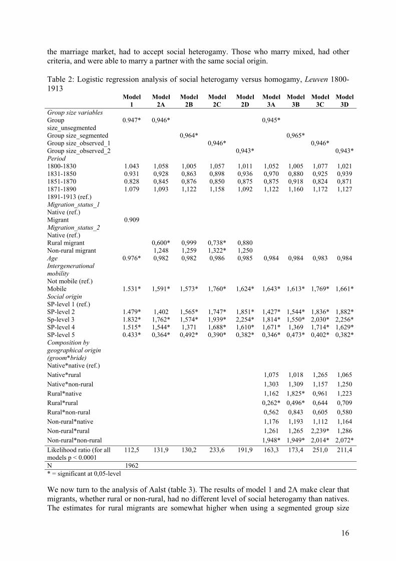
model 3B includes the segmented group variable, model 3C and 3D the observed group size variables. A first observation is that rural unmixed couples indeed show a very high level of homogamy (model 3A). The results of model 3B show that controlling for the segmented group sizes does not completely explain this high level of social homogamy. Yet, the results of model 3C and D, that provide the most strict criteria, show that, while homogamy is rather high, the estimates are no longer significant. What are possible factors enhancing social homogamy among rural migrants? It seems that middle class sons and daughters, by far the largest group among rural migrants, seem very keen on intermingling with similars, both in respect to social and geographical background. They share a rural, farming background. Being challenged by the same risks – life in the city, downward social mobility – it seems that the only possibility for them to find a decent and reliable partner is to confine themselves to other members of the rural middle class. The choice to marry a partner with the same geographical background is in a way a choice for homogamy (Van de Putte et al. 2005: 190). For these unmixed couples, it is very well possible that a choice for a market is induced by a wish to prevent downward marital mobility. If that is correct, controlling for the byproduct is far too strict, as it assumes that geographical homogamy happens before partner selection deliberations in terms of social origin. There is, perhaps, another argument not to control for the byproduct-effect. If we compare the social profile of rural migrants that marry other rural migrants with that of those who marry natives or non-rural migrants, we see a difference. SP-level 4 is over-represented among the rural unmixed (72% compared to 52% among natives). This can, perhaps, be explained as the consequence of a status preservation strategy among these rural middle class (threatened by downward social mobility). Yet, at the same time, it does not seem to be the case that geographical homogamy is the pure product of social homogamy. Rural migrants in SP-level 4 who marry homogamous according to social origin have a preference for rural migrants: 62% of their partners are rural migrants, while the proportion of rural migrants in SP-level 4 is only about 34%. In our view, all this means that SP-level 4 sons and daughters indeed were keen on social homogamy (what explains their over-representation among the rural unmixed couples), but they were especially keen do this when it was combined with geographical homogamy. To sum up, in a conservative approach, we would state that while there are indications that the high level of social homogamy is not simply the product of being isolated on the marriage market (status preservation strategy of rural migrants, rather high but not always significant levels of social homogamy in each model), the results are not hard enough to confirm this. Perhaps the most precise interpretation is that rural migrants were very willing to accept the consequences of the byproduct-effect. Second, there is, perhaps, some evidence for an exchange-effect. Rural migrants marrying a native bride have more chance to marry heterogamous (model 3B). In practice, this often meant downward marital mobility, as 41% of the rural men marrying a native bride was downwardly mobile, compared to 20% for rural men marrying a rural migrant bride.7 But the 7 Yet, we do not find this for rural migrant brides marrying a native groom (in crude figures, about 32% of rural migrant brides married downward). This would suggest that the need for integration is typically strongest for men – they have to accept downward marriage, while the couple's integration apparently is not hindered by the migration status of the bride. Although this sounds plausible, it remains a topic under discussion.

14

estimates of model 3B are based on the rural marriage market. This means that compared to homogamy levels that can be expected in case these people were confined to the rural migrant marriage market, they are quite heterogamous. Yet, when considering more realistic group sizes, this effect is no longer present. The situation is somewhat different if we use the unmixed rural migrant couples instead of the unmixed native couples as the reference group (data not shown). In that case, rural grooms marrying native brides are in every model more heterogamous compared to rural grooms marrying rural brides, although in model 4C the parameter is not significant (1,493; p = 0,18).8 Also concerning this exchange effect, the conservative interpretation is that there are not enough hard indications that it is really present – even though social heterogamy is quite high for rural migrants marrying native brides (but not significant in model 3C). Let us consider the first and second observation together. It is clear that choosing a specific niche of the marriage market may include effects in terms of social homogamy. If one knows that marrying a native partner in practice implies downward mobility – even though it might be stimulated by structural factors – deciding to marry one is the same as deciding to pay the price of integration. At the same time, if one knows that marrying a migrant partner is usually the same as marrying homogamous, to limit oneself to the rural migrant marriage market is, it would seem, a choice for the preservation of one's status. By holding a conservative line of interpretation, we stated that there is not enough evidence that the observed patterns were really caused by strategies in terms of social origin. Doing this, is the same as stating that they were the product of structure, in this case the segmentation of the marriage market by geographical origin. We are fully aware that the reader may find this choice somewhat arbitrary. To sum up, the choice is up to the researcher: do we believe in structure? Or in agency? Third, in every model unmixed non-rural couples have a high level of heterogamy. Although this is a rather small group, the pattern is striking (and significant). At first sight, we would not expect a Blau-effect here, as these non-rural migrants are less strongly avoided by the natives, and therefore, in theory, they have a rather large group of potential marriage partners at their disposal. However, there might be a selection-effect here. It cannot be excluded that the group of non-rural unmixed couples was that part of the non-rural migrants that was rather attached to its non-rural migrant status. Yet, assuming that this was indeed the case should, in our view, at least be based on the observation of some specific characteristics of this group, e.g. in terms of their specific region of descent. A large part of these non-rural unmixed are born in a French-speaking region or abroad (together about 30 to 40%). Yet it is not this group this is most heterogamous, on the contrary, it is the group of Flemish non-rural migrants that is heterogamous. The only explanation we can think of is that for them the Blau-effect counts. They wanted to – or had to – marry with an in-group member. Those who marry unmixed are too migrant to be integrated in the native community, while they are too non-rural to be attached to the rural community. And as their group size is small, it is impossible to find a partner with the proper social origin. They, constrained as they were to their niche of

8 Also in this niche of the marriage market (rural grooms marrying native brides) we do find some differences in the social structures compared to the general social structures. But these do not show any strategy that may explain the exchange effect. Native brides marrying a rural groom, are more likely to be a SP-level 4 daughter (and less likely to be a SP-level 3 daughter) compared to those who marry a native groom. These are not the ones who look for an exchange marriage, as they are not likely to marry upwards – but they are likely to marry homogamous. Rural migrant grooms are less likely to be SP-level 4 than those rural grooms that marry rural brides, but also this can not be explained in terms of the exchange-effect.

15

the marriage market, had to accept social heterogamy. Those who marry mixed, had other criteria, and were able to marry a partner with the same social origin. Table 2: Logistic regression analysis of social heterogamy versus homogamy, Leuven 1800-1913 Model

1 Model

2A Model

2B Model

2C Model

2D Model

3A Model

3B Model

3C Model

3D Group size variables Group size_unsegmented

0.947* 0,946* 0,945*

Group size_segmented 0,964* 0,965* Group size_observed_1 0,946* 0,946* Group size_observed_2 0,943* 0,943* Period 1800-1830 1.043 1,058 1,005 1,057 1,011 1,052 1,005 1,077 1,021 1831-1850 0.931 0,928 0,863 0,898 0,936 0,970 0,880 0,925 0,939 1851-1870 0.828 0,845 0,876 0,850 0,875 0,875 0,918 0,824 0,871 1871-1890 1.079 1,093 1,122 1,158 1,092 1,122 1,160 1,172 1,127 1891-1913 (ref.) Migration_status_1 Native (ref.) Migrant 0.909 Migration_status_2 Native (ref.) Rural migrant 0,600* 0,999 0,738* 0,880 Non-rural migrant 1,248 1,259 1,322* 1,250 Age 0.976* 0,982 0,982 0,986 0,985 0,984 0,984 0,983 0,984 Intergenerational mobility

Not mobile (ref.) Mobile 1.531* 1,591* 1,573* 1,760* 1,624* 1,643* 1,613* 1,769* 1,661* Social origin SP-level 1 (ref.) SP-level 2 1.479* 1,402 1,565* 1,747* 1,851* 1,427* 1,544* 1,836* 1,882* Sp-level 3 1.832* 1,762* 1,574* 1,939* 2,254* 1,814* 1,550* 2,030* 2,256* SP-level 4 1.515* 1,544* 1,371 1,688* 1,610* 1,671* 1,369 1,714* 1,629* SP-level 5 0.433* 0,364* 0,492* 0,390* 0,382* 0,346* 0,473* 0,402* 0,382* Composition by geographical origin (groom*bride)

Native*native (ref.) Native*rural 1,075 1,018 1,265 1,065 Native*non-rural 1,303 1,309 1,157 1,250 Rural*native 1,162 1,825* 0,961 1,223 Rural*rural 0,262* 0,496* 0,644 0,709 Rural*non-rural 0,562 0,843 0,605 0,580 Non-rural*native 1,176 1,193 1,112 1,164 Non-rural*rural 1,261 1,265 2,239* 1,286 Non-rural*non-rural 1,948* 1,949* 2,014* 2,072* Likelihood ratio (for all models p < 0.0001

112,5 131,9 130,2 233,6 191,9 163,3 173,4 251,0 211,4

N 1962 * = significant at 0,05-level

We now turn to the analysis of Aalst (table 3). The results of model 1 and 2A make clear that migrants, whether rural or non-rural, had no different level of social heterogamy than natives. The estimates for rural migrants are somewhat higher when using a segmented group size

16

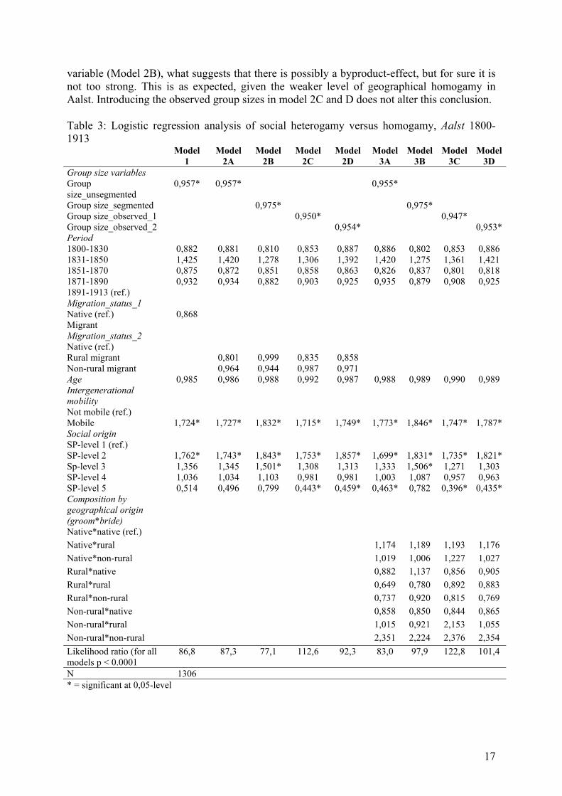
variable (Model 2B), what suggests that there is possibly a byproduct-effect, but for sure it is not too strong. This is as expected, given the weaker level of geographical homogamy in Aalst. Introducing the observed group sizes in model 2C and D does not alter this conclusion. Table 3: Logistic regression analysis of social heterogamy versus homogamy, Aalst 1800-1913 Model

1 Model

2A Model

2B Model

2C Model

2D Model

3A Model

3B Model

3C Model

3D Group size variables Group size_unsegmented

0,957* 0,957* 0,955*

Group size_segmented 0,975* 0,975* Group size_observed_1 0,950* 0,947* Group size_observed_2 0,954* 0,953* Period 1800-1830 0,882 0,881 0,810 0,853 0,887 0,886 0,802 0,853 0,886 1831-1850 1,425 1,420 1,278 1,306 1,392 1,420 1,275 1,361 1,421 1851-1870 0,875 0,872 0,851 0,858 0,863 0,826 0,837 0,801 0,818 1871-1890 0,932 0,934 0,882 0,903 0,925 0,935 0,879 0,908 0,925 1891-1913 (ref.) Migration_status_1 Native (ref.) 0,868 Migrant Migration_status_2 Native (ref.) Rural migrant 0,801 0,999 0,835 0,858 Non-rural migrant 0,964 0,944 0,987 0,971 Age 0,985 0,986 0,988 0,992 0,987 0,988 0,989 0,990 0,989 Intergenerational mobility

Not mobile (ref.) Mobile 1,724* 1,727* 1,832* 1,715* 1,749* 1,773* 1,846* 1,747* 1,787* Social origin SP-level 1 (ref.) SP-level 2 1,762* 1,743* 1,843* 1,753* 1,857* 1,699* 1,831* 1,735* 1,821* Sp-level 3 1,356 1,345 1,501* 1,308 1,313 1,333 1,506* 1,271 1,303 SP-level 4 1,036 1,034 1,103 0,981 0,981 1,003 1,087 0,957 0,963 SP-level 5 0,514 0,496 0,799 0,443* 0,459* 0,463* 0,782 0,396* 0,435* Composition by geographical origin (groom*bride)

Native*native (ref.) Native*rural 1,174 1,189 1,193 1,176 Native*non-rural 1,019 1,006 1,227 1,027 Rural*native 0,882 1,137 0,856 0,905 Rural*rural 0,649 0,780 0,892 0,883 Rural*non-rural 0,737 0,920 0,815 0,769 Non-rural*native 0,858 0,850 0,844 0,865 Non-rural*rural 1,015 0,921 2,153 1,055 Non-rural*non-rural 2,351 2,224 2,376 2,354 Likelihood ratio (for all models p < 0.0001

86,8 87,3 77,1 112,6 92,3 83,0 97,9 122,8 101,4

N 1306 * = significant at 0,05-level

17

The results of model 3A, B, C and D show that there were no strong differences in social heterogamy for couples compared by their composition by geographical origin. This is also in line with the expectations, as, for example, the Blau- and exchange-effect are based on the idea that some avoidance of migrants existed, what was not really the case in Aalst. To sum up, there is no segmentation of the marriage market by geographical origin that is strong enough to influence the results dramatically. The results may also shed some light on the situation in Leuven. Also in Aalst there is a different social structure for rural migrants than for natives (although less outspoken than in Leuven). Therefore, also in Aalst there was the possibility for rural migrants to use the same strategy as in Leuven: to marry other rural migrants to prevent downward social mobility. But we do not really find that pattern in Aalst. Apparently, they did not do so. If this status preservation strategy is that important that it brings people to geographical homogamy, what could be the conclusion looking at the Leuven results, why then would it be that different in Aalst? Of course, we cannot exclude that in Leuven there was more need for such a strategy - although we do not have indications that this indeed would be the case. Yet, in our view, the findings for Aalst suggest that the pattern found in Leuven was also not (only) the product of this active agent looking for status preservation. It was probably the product of the segmentation of the marriage market by geographical homogamy. Finally we turn the results for Gent (table 4). The results of model 1 are similar as in Leuven and Aalst. Migrants do not have a different level of social homogamy than natives. Model 2A again shows the necessity to distinguish between rural migrants and non-rural migrants. Although the estimates for these categories are not significantly different from the native reference group, it is quite clear that the two migrant groups have different levels of social homogamy (significant in case one of the migrant groups is the reference category). Mind that the direction is different from what we observed in Leuven. Rural migrants have higher levels of heterogamy than non-rural migrants. The results for model 2B are revealing. Controlling for the byproduct-effect, the estimates for rural migrants are indeed significantly different from natives. This means that the high level of social heterogamy of rural migrants was suppressed by the byproduct-effect. Again, and this is of course not unexpected, the byproduct-effect does not really affect the pattern of homogamy of non-rural migrants. These patterns also appear in case we use the observed group size variables (model 2C and D). So, in both Leuven and Gent we find a high level of geographical homogamy and a byproduct-effect, while in Aalst geographical homogamy is lower, and there is no byproduct-effect. In our view, there are more reasons to believe that this geographical homogamy is independent from strategies in terms of social homogamy. Rural migrants are less similar than natives in Gent and Leuven, and that is why we find geographical homogamy there and not in Aalst, where they are rather similar to the inhabitants. An explanation for the relatively high level of homogamy among rural migrants in terms of strategies of social homogamy (instead of the structural byproduct-effect) is less likely to be correct, as there is no indication why this status preservation strategy is stronger in Leuven and Gent compared to Aalst. In other words, we have only one solid argument to explain the differences between Leuven and Gent on one side and Aalst at the other side, and that argument leads us to choose for the byproduct-effect as the explanation.

18

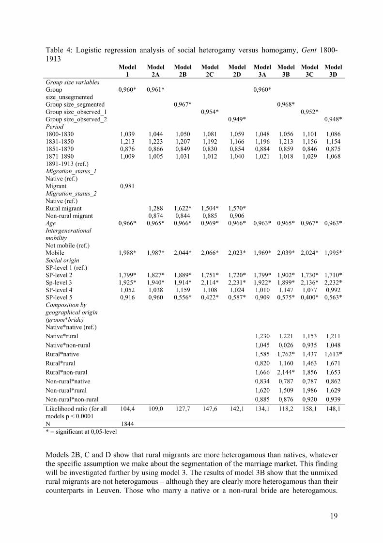
Table 4: Logistic regression analysis of social heterogamy versus homogamy, Gent 1800-1913 Model

1 Model

2A Model

2B Model

2C Model

2D Model

3A Model

3B Model

3C Model

3D Group size variables Group size_unsegmented

0,960* 0,961* 0,960*

Group size_segmented 0,967* 0,968* Group size_observed_1 0,954* 0,952* Group size_observed_2 0,949* 0,948* Period 1800-1830 1,039 1,044 1,050 1,081 1,059 1,048 1,056 1,101 1,086 1831-1850 1,213 1,223 1,207 1,192 1,166 1,196 1,213 1,156 1,154 1851-1870 0,876 0,866 0,849 0,830 0,854 0,884 0,859 0,846 0,875 1871-1890 1,009 1,005 1,031 1,012 1,040 1,021 1,018 1,029 1,068 1891-1913 (ref.) Migration_status_1 Native (ref.) Migrant 0,981 Migration_status_2 Native (ref.) Rural migrant 1,288 1,622* 1,504* 1,570* Non-rural migrant 0,874 0,844 0,885 0,906 Age 0,966* 0,965* 0,966* 0,969* 0,966* 0,963* 0,965* 0,967* 0,963* Intergenerational mobility

Not mobile (ref.) Mobile 1,988* 1,987* 2,044* 2,066* 2,023* 1,969* 2,039* 2,024* 1,995* Social origin SP-level 1 (ref.) SP-level 2 1,799* 1,827* 1,889* 1,751* 1,720* 1,799* 1,902* 1,730* 1,710* Sp-level 3 1,925* 1,940* 1,914* 2,114* 2,231* 1,922* 1,899* 2,136* 2,232* SP-level 4 1,052 1,038 1,159 1,108 1,024 1,010 1,147 1,077 0,992 SP-level 5 0,916 0,960 0,556* 0,422* 0,587* 0,909 0,575* 0,400* 0,563* Composition by geographical origin (groom*bride)

Native*native (ref.) Native*rural 1,230 1,221 1,153 1,211 Native*non-rural 1,045 0,026 0,935 1,048 Rural*native 1,585 1,762* 1,437 1,613* Rural*rural 0,820 1,160 1,463 1,671 Rural*non-rural 1,666 2,144* 1,856 1,653 Non-rural*native 0,834 0,787 0,787 0,862 Non-rural*rural 1,620 1,509 1,986 1,629 Non-rural*non-rural 0,885 0,876 0,920 0,939 Likelihood ratio (for all models p < 0.0001

104,4 109,0 127,7 147,6 142,1 134,1 118,2 158,1 148,1

N 1844 * = significant at 0,05-level Models 2B, C and D show that rural migrants are more heterogamous than natives, whatever the specific assumption we make about the segmentation of the marriage market. This finding will be investigated further by using model 3. The results of model 3B show that the unmixed rural migrants are not heterogamous – although they are clearly more heterogamous than their counterparts in Leuven. Those who marry a native or a non-rural bride are heterogamous.

19

This looks like evidence for the exchange-effect.9 However, if we test the exchange-effect by including observed group sizes (model 3C and D), the estimates become insignificant – while still high. Furthermore, in these models, the level of homogamy of rural migrants is not different for those who marry natives, non-rural migrants or rural migrants. In other words, rural migrants are heterogamous in any case. This is different from what we observed in Leuven. A factor that might explain the high level of heterogamy of rural migrant unmixed couples is the difference in relative size of the group of rural migrants in both cities. In Gent, this group is much smaller (one third of migrants are rural, while one on two in Leuven), and this makes it more difficult to combine it with social homogamy (Blau-effect). Conclusion In the theoretical section we formulated three propositions concerning the impact of the segmentation of the marriage market on marital mobility. The first proposition was that 'migrants who are avoided and who have a different social structure, will show high levels of social homogamy because of the byproduct-effect'. In our interpretation, the results of this paper support the proposition. The rural migrants of Leuven and Ghent are avoided and have a specific social profile. In Leuven their level of social homogamy was high, and became less high when controlling for the byproduct-effect. In Gent, their level of social homogamy was not high, but became even less high when controlling for the byproduct-effect. The second proposition was that 'migrants who are avoided, will have high levels of social heterogamy in case they marry with natives because of the exchange-effect'. We did not find much support for this proposition in our analysis, although the tests we performed were rather strict. The third proposition was that 'migrants and (particularly) natives who see geographical origin as their priority criterion, will have a higher level of social heterogamy as it is difficult to combine their priority with other criteria (Blau-effect). This will be particularly the case for small groups.' The conditions in Leuven, Gent and Aalst were not very favourable for this effect. Nevertheless, some findings can be interpreted as support for this proposition. The high level of social heterogamy of rural migrants in Gent, and of non-rural migrants in Leuven, are examples. Altogether, in our interpretation, the analyses performed in this paper lead to an important conclusion: group formation according to geographical origin can lead to the segmentation of the marriage market. And this segmentation may influence patterns of social mobility. First, it complicates the relation between migration and marital mobility. It is necessary to distinguish between migrants who are seen as members of an out-group and migrants who are more closely connected to the native city inhabitants. The first group will be avoided, and this will lead to a series of effects. There may be strong structural effects (e.g. the byproduct-effect), but the structural conditions may also be the starting point of strategies in terms of marital mobility (e.g. the Blau-effect). Second, trends of marital mobility over time and differences between societies might be influenced by changes and differences in the strength of the segmentation of the marriage market. Societies characterised by a strong byproduct-effect

9 Again, there is no such an effect for natives or non-rural grooms marrying a rural bride. For the time being, we ignore this gender-effect.

20

may have higher levels of social homogamy, and, depending on the precise research question, it might be necessary to control for it. We have to admit that our methodology and interpretation are not beyond criticism. The methodology has disadvantages, in that sense that each variant model that aims to control for marriage market characteristics is based on assumptions that are not easy to test. As a consequence, our interpretation of marriage patterns is not only based on the results obtained by using this methodology, but also on an appreciation of how human behaviour is shaped. It remains, for example, an open question to what extent human behaviour can surmount the structure of the marriage market. Consequently, it remains an open question to what extent we have to control for the characteristics of the marriage market. At the other hand, we do think that the proposed method is useful to start the search for an explanation of the relation between migration and marital mobility in terms of the segmentation of the marriage market by geographical origin. Finally, it is needless to say that many issues remain open for debate. Some examples are the influence of the migrant's social origin on the segmentation of the marriage market, and the difference between male and female migrants. Bibliography Alter, G. (1988) Family and the female life course. The women of Verviers, Belgium, 1849-1880. Madison: The University of Wisconsin Press. Beekink, E., Liefbroer, A., & Van Poppel, F. (1998) Changes in choice of spouse as an indicator of a society in a state of transition: Woerden, 1830-1930. Historical Social Research, 22, 231-253. Blau, P., Beeker, C., & Fitzpatrick, K. (1984) Intersecting social affiliations and intermarriage. Social Forces, 62, 585-606. Bras, H. (1998) Domestic Service, Migration and the Social Status of Women at marriage. The Case of a Dutch Sea Province, Zeeland 1820-1935. Historical Social Research, 23, 3, pp.3-19. Bras, H. & Kok, J. "They Live in Indifference Together": Marriage Mobility in Zeeland, The Netherlands, 1796-1922. International Review of Social History, vol. 50, supplement 13, pp.247-274. Dribe, M., Manfredini, M., Oris, M. & Neven, M. (2005) Marriage and migration in a comparative European perspective, paper presented at the annual meeting of the Social Science History Association, Portland Oregon. Jacquemin, A. (1998b) Modernisation de la nuptialité et différaciation sociale dans une métropole urbaine. Liège entre 1840 et 1890. In: C. Desama & M. Oris, Dix essais sur la démographie urbaine de la Wallonie au XIXe siècle. Bruxelles: Crédit Communal, (pp. 197-241). (Collection Histoire in-8°, nr 98). Kalmijn, M. (1998) Intermarriage and homogamy: causes, patterns, trends. Annual Review of Sociology, 24, 395-421. Kasakoff, A., Adams, J. (1995) The effect of migration on ages at vital events: a critique of family reconstitution in historical demography. European Journal of Population/Revue Européenne de Démographie, 11, 3, pp.199-242. Kennedy, R. (1944) Single or Triple Melting-Pot? Intermarriage Trends in New Haven, 1870-1940. The American Journal of Sociology, 46, 4, pp.331-339.

21

Klesman, C. (1987) Long-distance migration, integration and segregation of an ethnic minority in industrial Germany: the case of the 'Ruhr Poles'. In: K. Bade (ed.), Population, labour and migration in 19th- and 20th-century Germany (pp. 101-114). Leamington Spa/Hamburg/New York: Berg. Mokyr, J. Industrialization in the Low Countries, 1795-1850, New Haven/London: Yale University Press, 1976. Oris, M. (2000) The age at marriage of migrants during the industrial revolution in the region of Liège. History of the Family, 5(4), 391-413. Oris M., Capron C., Neven M., Le poids des réseaux familiaux dans les migrations en Belgique orientale qu 19e siècle. Peut-on quantifier? In: E. Sonnino (ed.), Living in the City, Rome: x, 2002:151-178. Schrover, M. (2004) 'De Duitscher is immers tegenwoordig ook zeer gallant voor dames'. Huwelijksgedrag van migranten in Nederland in de 19e eeuw. Bevolking en Gezin, 33, 2, pp.103-126. Sewell, W. (1976) Social mobility in a nineteenth-century European city: some findings and implications. Journal of Interdisciplinary History, 7(2), 217-233. Shanahan, S., & Olzak, S. (1999) The effects of immigrant diversity and ethnic competition on collective conflict in urban America: an assessment of two moments of mass migration, 1869-1924 and 1965-1993. Journal of American Ethnic History, 18(3), 40-64. Uunk, W. (1996) Who marries whom? The role of social origin, education and high culture in mate selection of industrial societies during the twentieth century. Nijmegen: Katholieke Universiteit Nijmegen (Doctoraal Proefschrift). Van de Putte, B. (2003) Homogamy by geographical origin. Segregation in 19th century Flemish cities (Leuven, Aalst and Ghent). Journal of Family History, 28(3), 364-390. Van de Putte B., Partnerkeuze in de 19de eeuw. Klasse, geografische afkomst, romantiek en de vorming van sociale groepen op de huwelijksmarkt, Leuven: Leuven University Press, 2005. Van de Putte B., Miles A. (2005), A class scheme for historical occupational data. The analysis of marital mobility in industrial cities in 19th century Flanders and England, Historical Methods, 38, 2, pp.61-92. Van de Putte B., Neven M., Oris M., Matthijs K. (2005), Migration, sector identity and societal openness in 19th century Belgium, International Review of Social History, vol. 50, supplement 13, pp.179-218. van Leeuwen, M., Maas, I., & Miles, A. (eds.) (2002) HISCO. Historical International Standard Classification of Occupations. Leuven: Leuven University Press. Wildsmith E., Gutmann M., Gratton B., Assimilation and Intermarriage for U.S. Immigrant Groups, 1880-1990, s.d. List of variables Unsegmented group size For groom x belonging to SP-level y in Period z the group size value is equal to the percentage of brides in SP-level y in Period z. Segmented group size For native groom x belonging to SP-level y in Period z the group size value is equal to the percentage of brides in SP-level y in Period z among the natives. For rural migrant groom x belonging to SP-level y in Period z the group size value is equal to the percentage of brides in SP-level y in Period z among the rural migrants. For non-rural migrant groom x belonging to SP-level y in Period z the group size value is equal to the percentage of brides in SP-level y in Period z among the non-rural migrants.

22

23

Observed group size_1 For groom x who married a native bride, and who belonged to SP-level y in Period z the group size value is equal to the percentage of brides in SP-level y in Period z among the natives. For groom x who married a rural migrant bride, and who belonged to SP-level y in Period z the group size value is equal to the percentage of brides in SP-level y in Period z among the rural migrants. For groom x who married a non-rural migrant bride, and who belonged to SP-level y in Period z the group size value is equal to the percentage of brides in SP-level y in Period z among the non-rural migrants. Observed group size_2 For grooms in an unmixed marriage, group size value = value for segmented group size variable. For grooms in an mixed marriage, group size value = value for unsegmented group size variable. Migration status_1

- native (reference category) - migrant

Period

- 1800-1830 - 1831-1850 - 1851-1870 - 1871-1890 - 1891-1913 (reference category)

Social origin groom

- SP-level 1 (reference category) - SP-level 2 - SP-level 3 - SP-level 4 - SP-level 5

Intergenerational social mobility

- mobile - immobile (reference category)

Age: Parametric variable. Migration status_2

- native (reference category) - rural migrant - non-rural migrant

Composition of the couple by geographical origin

- Native groom marrying native bride - Native groom marrying rural migrant bride - Native groom marrying non-rural migrant bride - Rural migrant groom marrying native migrant bride - Rural migrant groom marrying rural migrant bride - Rural migrant groom marrying non-rural migrant bride - Non-rural groom marrying native migrant bride - Non-rural groom marrying rural migrant bride - Non-rural groom marrying non-rural migrant bride