Embed Size (px)
Citation preview

The Service Sector and Female Market Work:
Europe vs US∗
Michelle Rendall†
The University of Zurich
January 22, 2013
ABSTRACT
This paper studies cross-country di�erences in female employment and aggregate labor market hours overtime, by quantifying the role of structural transformation and gender di�erences in sectoral labor produc-tivity. Some countries have developed large service sectors, while others have not. These sectoral patternscan explain a large part of the cross-country di�erences in female employment and aggregate hours worked.Empirical evidence on why women predominately work in the service sector is provided. Consistent withprevious studies, labor and consumption tax di�erences are able to explain large sectoral di�erences acrosscountries. The key is households can produce a substitute for market services and women are, on average,less productive in sectors requiring more brawn, such as industry, giving them a comparative advantageto stay at home and work in the service sector. Therefore, an economy that imposes high taxes does notfacilitate the movement of women into the labor market, causing service production to remain at home.This reduces the demand for market services, which feeds back into low total hours worked by women (andthe total economy). Subsidies to female employment can circumvent the high tax e�ect, but lead to welfareloses.
JEL classi�cation: E21, E24, J20.Keywords: technological progress, sectoral labor allocation, cross-country di�erences, female labor supply,labor demand/supply, taxation.
∗I would like to thank, seminar and conference participants at Minneapolis Federal Reserve, New York University,SED Conference in Ghent, University of Zurich, Virginia Tech, and World Bank for valuable comments. Financialsupport from the European Research Council (ERC Advanced Grant IPCDP-229883) is gratefully acknowledged.†University of Zurich, Department of Economics, Muehlebachstrasse 86 CH-8008 Zurich.
Email: [email protected]. All errors are mine.

1 Introduction
Cross-country di�erences of hours worked in OECD countries since 1960 has been studied exten-
sively. Tax di�erences are often posited as the main force leading to discrepancies in cross-country
hours worked (Prescott, 2004), productivity di�erences (Rogerson, 2008), and the substitution of
market to home production (Ragan, 2006; Rogerson, 2008; Olovsson, 2009). This research mod-
els the household as a single representative agent. However, McDaniel (2010) �nds that changes in
market work and home production vary to a large extent when disaggregated by sex, after analyzing
time-use survey data across developed countries. This fact is particularly interesting in the context
of one of the greatest phenomena of the 20th century, the rise in female labor force participation.
This phenomena, however, has not been uniform, with Continental Europe experiencing a smaller
rise in formal female employment compared with the US or the Nordic countries.1 The goal of this
paper is to quantify the importance of sectoral labor reallocation and productivity di�erences in the
rise of female employment and cross-country di�erences in aggregate hours worked.
To explain the large cross-country female employment di�erences, and its correlation with the
service sector size, empirical evidence giving weight to a demand side (technology) story is provided.
As with prior research, the model quanti�es the importance of taxation and productivity in explain-
ing aggregate hours worked. While there is a large body of related literature, the present exercise
is useful for various reasons. Bick and Fuchs-Schündeln (2012) focus on a large set of countries to
explain contemporaneous labor supply di�erences through taxes and Ngai and Petrongolo (2012)
focus on the long run trends in the US and changes in structural transformation. Here both these
topics are combined. Focusing on tax di�erences, structural transformation, and the entrance of
women into the labor force in one model allows us to disentangle the contribution of each these
facts in the fall (rise) of total hours worked, the size of the service sector, and gender employment
di�erences.
Recent research has concluded that di�erences in total employment have come from a falling
goods sector's (industry and agricultural sector) employment share relative to the US and higher
income tax rates (see Rogerson, 2008). While tax rates have increased in all of the developed
1Given data availability, this study compares Germany, Sweden, and the US.
2

world since 1960, Continental Europe generally employes much higher tax rates, shifting hours from
the market to the home. In contrast, Scandinavia has high taxes, but subsidizes market services
such as childcare and elderly care. Some of the subsidies in Scandinavia are speci�cally target
at working mothers, with generous maternity leave and comprehensive childcare. In productivity
di�erences, Continental Europe has a substantially smaller service sector. The correlation between
relative female employment change and aggregate service employment is around 0.82 from the 1980s
onward for a large set of OECD countries (Rogerson, 2005). Rogerson (2008) �nds when comparing
aggregate employment between the US and Europe, most of the discrepancy is accounted for by
di�erences in service sector employment. While there are small employment di�erentials in industry
(slightly positive), Europe has an employment di�erential in services of -9.4 percent in the mid-
1950s and -15.5 percent in 2000 compared to the US. Rendall (2010) provides empirical results
for the United Sates showing that job requirements have shifted from physical attributes toward
intellectual attributes since WWII, bene�ting women through greater job opportunities, higher
wages and increasing returns to education. A large portion of the decrease in physical requirements
is due to a shift toward services, and away from heavy manufacturing, agriculture and mining.
This study develops a general equilibrium model based on the following three facts regarding
the US, German and Swedish labor supply and sectoral labor allocation over time speci�cally.2
1. Service sector employment has increased in all developed countries. While Sweden and the
US have similar employment trends, a sizable gap with Germany persists.
2. American women's labor force participation, age 15-64, rose from about 40 to 67 percent from
1960 to 2000. Sweden also has large female employment rates of 71 percent in 2000. However,
Germany's female employment has only risen to 58 percent.
3. American men's labor force participation age 15-64, fell from about 82 to 78 percent from
1960 to 2000. The fall in Germany was 20 percentage points and 17 in Sweden.
Figure 1 provide trends over time in relative sectoral hours and aggregate hours. Female hours have
o�-set the fall in the of men's working hours in the US and Sweden, but not in Germany.
2Figures on employment rates are taken from the OECD database. Sectoral labor allocations are taken from theGroningen Growth and Development Centre 10-Sector database and EU KLEMS Database.
3

0.4
0.5
0.6
0.7
0.8
Fra
ctio
n E
mp
loy
ed
in
Se
rvic
es
0
0.1
0.2
0.3
1960 1965 1970 1975 1980 1985 1990 1995 2000
Fra
ctio
n E
mp
loy
ed
in
Se
rvic
es
USA DEU SWE
(a) Relative Sectoral Hours
0.15
0.2
0.25
0.3
0.35
((A
nn
ua
l Ho
urs
Wo
rke
d)/
52
00
)/P
op
ula
tio
n (
Ag
e 1
5-6
4)
0
0.05
0.1
1960 1965 1970 1975 1980 1985 1990 1995 2000
((A
nn
ua
l Ho
urs
Wo
rke
d)/
52
00
)/P
op
ula
tio
n (
Ag
e 1
5
USA DEU SWE
(b) Hours Evolution
Source: OECD database, 10-Sector database, EU KLEMS database
Figure 1: Employment Across Countries
Given the empirical evidence, a general equilibrium model is developed to understand the evo-
lution of female and male employment within the broad rise of the service sector. Men are assumed
to have equal productivity across all sectors, while women's average productivity in each sector is
taken from wage gap data. Similar to Ngai and Pissarides (2008), households allocate time between
the home and labor market, and choose consumption over three types of goods: market produced
services, market produced goods and home produced goods/services. The model has two key as-
sumptions. Similar to Rogerson (2008), households can produce a substitute for market produced
services (e.g., childcare, elderly care, meals) using home production technology and labor time.
Second, given US and European wage gap estimates, women have higher productivity in the service
sector. Therefore, women generally prefer working in the service economy where occupations neither
require great physical strength nor have adverse working environments.
In combining both taxes and structural transformation e�ects over time some simpli�cations are
made compared to Bick and Fuchs-Schündeln (2012) and Ngai and Petrongolo (2012). While the
former model di�erent tax issues (e.g., average versus marginal) in detail, this paper uses represen-
tative households and an average tax measure. Ngai and Petrongolo (2012) model an endogenous
wage gap to determine the quantitative contribution of structural change to female employment
4

and wages. They �nd structural change can only explain a small part of the rise in female wages.
Here, the closing wage gap is taken as exogenous, whether it is due to compositional e�ects, i.e.,
human capital as in Ngai and Petrongolo (2012), or a fall in discrimination. These simpli�cations
allow the model to highlight the di�erences that have pushed women into the labor market. Most
of the literature accounting for the rise in female labor force participation has focused on supply
driven stories, i.e., improvements in home technology, such as the invention and marketization of
household appliances (see, for example, Greenwood, Seshadri, and Yorukoglu, 2002, and references
therein), the improvements in baby formulas (see Albanesi and Olivetti, 2006), rising female wages
(see Jones, Manuelli, and McGrattan, 2003) and returns to experience (see Olivetti, 2006), or the
e�ects of cultural, social, and intergenerational learning on labor supply (see Fernandez, 2007; Fogli
and Veldkamp, 2007). Here, the rise in female labor force participation is driven by changes in mar-
ket productivity (a shrinking wage gap) due to sectoral reallocation, changes in home productivity,
and di�erences in taxes and subsidies.
The model is calibrated to match the growth experience of the US from 1960 to 2000. This study
initially quanti�es how much of the rise in female employment can account for the rise in the service
sector, and how important structural change versus the closing gender gap is in accounting for the
rise in female employment. Using the calibrated economy of the US, the higher tax implication can
be analyzed. That is, how much would female employment have grown in the US with German style
taxes and how large would the service sector have been? Furthermore, the di�erences between the
US (low taxes) and the Swedish systems (high taxes and subsidized market services) with respect to
social welfare loses are assessed in the context of the model by setting a subsidy to services, which
is tied to women's labor force participation, that matches female employment levels in the US.
From the features of woman's sectoral productivity and home substitution, a rich set of dynamic
results are presented, which are capable of generating both a convergence in female and male labor
market outcomes and a rise in the service sector, if taxes remain low. That is, an economy that
does not initially facilitate the movement of women into the labor market by, for example, impos-
ing high taxes without the social bene�ts tied to working women in Scandinavia (e.g., subsidized
full-day child care, elderly care) causes the production of services to remain in the home. As a
5

result, women do not enter the workforce and the growth of the service sector outside the home is
considerably slowed. About half of the rise in service sector employment in the US is explained by
the feedback e�ect of more women entering the labor market. Working women produce less services
at home and, therefore, purchase more market services, increasing the demand for services. The
high-tax Scandinavian system generates equally large female employment rates and service sector
employment, but with a larger welfare cost compared to the US, through a tax-subsidy distortion.
As women's productivity across sectors and changes in labor demand are the key motivations
within this study, Section 2 provides a brief summary on the changing labor market. The general
equilibrium model is outlined in Section 3, and Section 4 provides analytical results of productivity
growth on labor supply, wages, and sectoral labor shares. Section 5 discusses the estimation and
calibration procedure, and presents labor market trends across regions resulting from di�erences in
taxation and work subsidies. Section 7 concludes.
2 Labor Market Requirements
In a related paper (see for details Rendall, 2010), job characteristics by the US census occu-
pation and industry classi�cations from the 1977 Fourth Edition Dictionary of Occupational Title
(DOT) and the 1991 Revised Fourth Edition Dictionaries of Occupational are reduced using prin-
ciple component analysis to summarize aggregate labor market requirements. The 1977 and 1991
DOT were developed by the US Department of Labor, who evaluated approximately 40 job re-
quirements for more than 12,000 occupations, documenting: (1) general educational development;
(2) speci�c vocational training; (3) required working aptitudes; (4) temperaments or adaptability
requirements; (5) physical strength requirements; and (6) environmental conditions. For example,
general educational development measures the formal and informal educational attainment required
to preform a job e�ectively by rating reasoning, language and mathematical development. Each
reported level is primarily based on curricula taught in the US, where the highest mathematical
level is advanced calculus, and the lowest level only requires basic operations, such as adding and
subtracting two-digit numbers. Speci�c vocational preparation is measured in the number of years
a typical employee requires to learn the job tasks essential to perform at an average level. Eleven
6

aptitudes required of a worker (e.g., general intelligence, motor coordination, numerical ability) are
rated on a �ve point scale. Ten temperaments required of a worker are reported in the DOT, where
the temperament type is reported without any numerical rating. An example of a temperament
is the ability to in�uence people in their opinions or judgments. Physical requirements include a
measure of strength required on the job, rated on a �ve point scale from sedentary to very heavy,
and the presence or absence of tasks such as climbing, reaching, or kneeling. Lastly, environmental
conditions measure occupational exposure (presence or absence) to environmental conditions, such
as extreme heat, cold and noise.
Factor analysis or principal component analysis, similarly to Ingram and Neumann (2006),
reduces the dimensionality of DOT job characteristics. That is, using principal component analysis,
a linear relationship between normally distributed broad skill categories and the DOT characteristics
is estimated from the associated correlation matrix. Using maximum likelihood estimation methods,
three factors (brain, brawn and motor coordination), are determined to be su�cient in capturing
the information contained in the 1977 and 1991 DOT characteristics.3 The aggregate factors are
merged with the 1960 US Census data and the 1968 to 2000 Current Population Survey (CPS)
data.4 Figure 2, which plots all 1977 occupational brain and brawn combinations by sector in 1970,
clearly depicts the di�erence in brain and brawn requirements across sectors. Similarly, Goldin
(1990) observes that as far back as the 1920s/1930s women made work choices based on the level
of brawn required, which usually meant women preferred service sector jobs.
Clerical work was cleaner and less strenuous than manufacturing work ... It is under-
standable why young women preferred o�ce work and why the growth of the clerical
sector would lead to the continued employment of women after marriage and childbear-
ing. ... If the considerable di�erence in the earnings of males and females in manufac-
turing was largely due to rewards to strength, then the replacement of brain for brawn
work should have evened starting salaries. ... Although the di�erence in starting salaries
implied by the earnings functions between unmarried male and female clerical workers
3For details on the estimation see Rendall (2010).4Census and CPS data is obtained from the IPUMS-USA (Ruggles, Alexander, Genadek, Goeken, Schroeder, and
Sobek, 2010) and the IPUMS-CPS project (King, Ruggles, Alexander, Flood, Genadek, Schroeder, Trampe, andVick, 2010).
7

Fabric Mills
Construction
0.4
0.5
0.6
0.7
0.8
0.9
1.0
1.1
Brawn
Industry and
Agriculture
Services
Electrical machinery
Banking and credit agencies
Educational services
-0.1
0.0
0.1
0.2
0.3
-0.1 0.0 0.1 0.2 0.3 0.4 0.5 0.6 0.7 0.8 0.9 1.0 1.1
Brain
Source: 1977 DOT and 1970 CPS.
Figure 2: Occupation Factor Requirements by Sector
was negligible, it was 47% in manufacturing. Extract from Goldin, Understanding the
Gender Gap (1992) pp. 108-109
This evidence gives strong support to the hypothesis of productivity di�erences across sector
employment rather than overall labor market discrimination. Decomposing gender wage gaps across
sectors and countries provides further evidence of women's higher productivity in the service sector.
Figure 3 graphs US median female wages by sector relative to median male wages in the economy
of individuals working at least 1,400 hours per year. The wage gap in services is consistently
smaller from 1968 to 2000. The di�erence between the service and industrial gap averages around
7.2 percentage points.5 The gender gap closes similarly for both sectors, which could explain why
structural change alone can only explain a small share of the closing wage gap. Cross-country results
from the GGDC EU KLEMS datasets provide similar results. The EU KLEMS data provides hours
information and labor compensation by aggregate age and education groups. The data only exists
for Germany post-1990 (Sweden is not available). The wage gap di�erences between the service and
5The wage gap in agriculture shows large �uctuations across time given the small number of observations, especiallyof women. Since, the female labor share in agriculture is close to zero, the results are omitted here.
8

0.3
0.4
0.5
0.6
0
0.1
0.2
1965 1970 1975 1980 1985 1990 1995 2000
Industry Services
Source: 1968 to 2000 CPS.
Figure 3: Gender Wage Gap by Sector
industrial sector for middle skilled individuals aged 15 to 29 in Germany is on average 6.9, similar
to the magnitude in the US. The general patterns hold for the older cohorts and other education
groups as well. However, middle skilled individuals account for the bulk of German labor force.
3 General Equilibrium Model
The simulated economy consists of a representative two person household, a man and a woman;6
two competitive production sectors, industry and services; and a government. Labor reallocation
is driven as in Rogerson (2008); Duarte and Restuccia (2010), by both non-homothetic preferences
and di�erential sectoral productivity growth.
6The rise in labor force participation was considerably greater for married women, thus the analytical modelfocuses on two person households. Adding single households does not result in further dynamics within the model,and does not a�ect any of the qualitative results. The simulation results will add single households to match thequantitative targets.
9

3.1 Government
The government, who solves a balanced budget, taxes individuals labor income at rate, τ (yield-
ing the underlying cross-country di�erences over time). Tax revenues are rebated to households as a
lump-sum transfer, T . The government also provides price subsidizes on market services, v, and/or
rebates service goods indexed to women's labor supply as in Ragan (2006), φ.
τ(wm,thm,t + wf,thf,t) = Tt + vps,tcs,t + φhf,t, (1)
where wm,t, wf,t are male and female wages detailed below and hm,t, hf,t are the respective labor
supplies.
3.2 Production
The competitive sectors only use labor to produce �nal services and industrial goods {Ys, Yi}. By
assumption, women are less productive in producing industrial goods than services (services require
less brawn). Moreover, women also face �general� discrimination, that is, women's productivity
levels are {τi, τs}, where τi < τs ≤ 1. The �nal sectoral output is linear in labor,
Yj,t = Aj,tLj,t for j = i, s (2)
where Lj,t is aggregate labor supply and Aj,t is total factor productivity for each sector j. Therefore,
normalizing wages to one, relative prices are proportional to total factor productivity pj,t = 1Aj,t
.
3.3 Household Preferences
Household members are indexed with the subscripts g ∈ {f,m} for their gender. The only
di�erence between gender is their market productivity. There is no bargaining in the households
and households solve a unitary utility u(C,L), by allocating labor time of both agents to the market,
home production, and leisure; purchasing goods, ci, and services, cs, in the market; and producing
home produced service-substitutes at home, cn. Since, there is no inter-temporal decision, the model
10

is a time-sequence of static maximization problems of,
max{ci,t,cs,t,hm,t,hf,t,nt}
log (Ct) + ψ`1−σt
1− σ(3)
s.t.
pi,tci,t + (1− v)ps,tcs,t = (1− τ)(wm,thm,t + wf,thf,t) + Tt, (4)
1 = hm,t + nm,t + `m,t, (5)
1 = hf,t + nf,t + `f,t, (6)
nt = nm,t + nf,t, (7)
where C is the consumption composite of services and goods (suppressing time subscripts), i.e.,
C = (aicεi + (1− ai)F (cs, cn)ε)
1ε , (8)
where F (cs, cn) is the service composite, i.e.,
F (cs, cn) = (ac (cs + φhf )η + (1− ac)cηn)1η , (9)
where cs = cs + φhf are the total market purchased services, both privately and rebated by the
government for female hours worked. Home production is linear in labor cn = Ann. Leisure of
spouses are assumed to be perfectly complimentary, i.e., husbands and wives prefer spending time
together when not engaged in work.7
3.4 Wages
Since women always prefer to work in services, the simulation assumes that only a fraction
λt = γhi,tht
of women �nd employment in the service sector, wherehi,tht
is employment share in
industry for the economy at time t. Finding an industry job is more likely when the industry sector
7The single household problem is identical, expect for leisure, where leisure is enjoyed by the single agent alone.
11

is larger. Since wages are normalized to one, and men have equal productivity in all sectors, the
wage gap equals,
Gap =τsh
fs,t + τih
fi,t
hfs,t + hfi,t, (10)
where hs,f,t are hours worked of women that have wages wf,t = τs and work in the service sector,
and hi,f,t are hours worked of women that have wages wf,t = τi < τs and work in the industrial
sector.
3.5 Decentralized Equilibrium
An equilibrium, given productivity {τs,t, τi,t}, market prices {pi,t, ps,t}, and government prices
{τ, v, φ}, consists of the time path of households' allocation {ci,t, cs,t, hm,t, hf,t, nt}, �rm output
{Yi,t, Ys,t} and government allocation {Tt} such that for all t:
1. {ci,t, cs,t, hm,t, hf,t, nt} solves the Household Problem (3);
2. {Tt} solves the government problem (1);
3. Markets clear, with
a The labor market, Lsj,t = Ldj,t for j = i, s; and
b The goods market, cj,t = Yj,t for all j = i, s.
4 Analytical Results
The �rm's problem is straight forward. Technical change in terms of total factor productivity,
a rise inAi,tAs,t
, leads to a fall in relative goods to service prices.
4.1 Household Optimization
For a household, the problem is similar to Ngai and Pissarides (2008). Speci�cally, the household
problem can be solved in steps. The household solves three intertemporal choices, starting with the
service consumption decision, proceeding to the goods consumption decision, and ending with the
12

leisure decision. Since men have a comparative advantage in the labor market, household members
specialize, with the man entering the labor market �rst. As such, we will only analyze the case of
nm = 0, i.e., women spend at least a fraction of their time in the labor market.8 Time subscripts
are omitted for all intertemporal decisions.
Composite Service Consumption
Households choose time to be allocated to home production, n, in maximizing (9) s.t. (4). The
resulting �rst order condition can be summarized in terms of relative market services to home
services,
cscn
=
(as
1− as
(pn
(1− v)ps+
φ
An
)) 11−η
, (11)
where pn is an implicit home production price pn =wf (1−τ)An
. As in Ngai and Pissarides (2008),
services are �marketized� if cscn
rises. The comparative statics for the �marketization� of services, if
market and home services are gross substitutes, 0 < η < 1, can be summarized as follows:
• ∂cs/cn∂τ < 0, that is, higher taxes discourage market work;
• ∂cs/cn∂τf
> 0, higher brain demand encourages female market work (τf = 1(s=1)τs + 1(s=0)τi);
• ∂cs/cn∂φ > 0, governments subsidies, e.g., on childcare for working mothers, encourages female
market work; and
• ∂cs/cn∂w/((1−v)ps) > 0, a fall in service prices through subsidies or technological progress through
higher wages, encourages female market work.
Composite Consumption/Industrial Goods Consumption
Next households maximize (8), the �nal composite consumption, by choosing ci. The �rst order
condition can be summarized as relative market service to goods consumption,
csci
=
(1− aiai
pi(1− v)ps
as
(cs
F (cs, cn)
) η−εη
) 11−ε
. (12)
8The case with nm > 0 is very similar, however, the implicit home production price will be di�erent in the twocases.
13

Again, we can look at the comparative statics with respect to the key parameters. If services and
goods are gross compliments, ε < 0 and service types are substitutes, 0 < η < 1:
• ∂cs/cics/F (cs,cn)
> 0, more service marketization leads to rise in relative market service consumption
as η−ε1−ε > 0;
• ∂cs/ci∂τ < 0, higher taxes, lead to lower service marketization and, therefore, relatively less
market service consumption (indirect e�ect through lower marketization, similarly this will be
true for a smaller brain demand);
• ∂cs/ci∂φ > 0, again through the indirect e�ect of marketization, the government can arti�cially
increase the relative service demand; and
• ∂cs/ci∂v > 0, with a price subsidy on all service goods, the government can increase the relative
services demand even further, through both an indirect e�ect through marketization and a
direct price e�ect.
To summarize the comparative statics between di�erent government actions, if a price subsidy is
equivalent to the work subsidy, and the government only employs one at a time. The relative service
share will be largest with the price subsidy and smallest without any subsidy, assuming the same
tax rate for all economies, i.e.,(csci
){v>0,φ=0}
>(csci
){v=0,φ>0}
>(csci
){v=0,φ=0}
.
In conclusion, large taxation will lead to a smaller service sector, as fewer women participate in
the formal labor market and less services are marketized. The government can a�ect the relative
sector demands by subsidizing consumption of services. However, a subsidy tied to women working
is less powerful.
Leisure
To conclude the intertemporal choices of the household, individuals choose leisure by maximizing
(3). The �rst order condition can be described in terms of relative leisure to consumption,
`σ
C=
1− acacai
piw(1− τ)(2− τ f ) + (1− v)psφ
( ciC
)1−ε(13)
14

where ` = `m = `f . Leisure is greater with government price and work subsidies given equal tax
rates. The Frisch elasticity of labor, is governed by σ, which is ηit = 1σ`ithit
for individual type i.
4.2 Sectoral Labor Shares
Using market clearing, household allocation, and assuming women only work in services, λ = 1,
labor shares in the economy are as follows,
LsLi
=csci
pspi
(14)
=
(1− aiai
as(1− v)
(cs
F (cs, cn)
) η−εη
) 11−ε (
AsAi
) ε1−ε
.
The labor share of services rise, with a faster relative productivity growth in industry, given ε < 0.
Moreover, marketization leads to a rise in service labor shares. Therefore, a rise in female wages
leads to a rise in female employment and higher marketization, which ultimately translates into a
rise in service sector employment.
In summary, this section shows that larger government taxation leads to a smaller service sector
and less female labor force participation. Less female labor force participation in turn leads to a
smaller service sector. In addition, low female wages also lead to less female employment and less
service employment. Governments can increase female labor force participation, and, therefore, also
the service labor share, by subsidizing female employment or the purchase of services. Subsidizing
female employment through a rebate in services has the added e�ect of increasing service employ-
ment, e.g., more childcare facilities do not only provide services for households, but also employment
opportunities for women.
5 Calibration
The model is calibrated to US tax rates and initial conditions are then adjusted to account for
di�erences between Germany and the US. It is assumed that the US has reached its steady state by
2000 (there is evidence of �attening female labor force participation and gender wage di�erence in
15

Table 1: Tax Rates
Year USA DEU SWE
1960 28.43 39.32 30.802000 41.26 58.17 60.59
∆2000−1960 12.83 18.85 29.79
the last few years). Therefore, the results simulate two steady states in 1960 and 2000.
Tax rates are taken from McDaniel (2007). All three regions have seen rising tax rates over
time. The increase has been larger in Europe. Average tax rates are computed using both income
and consumption tax rates, i.e.,
τ = 1− 1− τh1 + τc
, (15)
where τh is the sum of the average tax rate on household income and the average payroll tax rate,
including both taxes paid by employer and employee, and τc is the average tax on consumption
expenditures. Table 1 summarizes the tax rates from each region in 1960 and 2000.
Table 2 summarizes the calibrated parameters. The parameter governing the elasticity of sub-
stitution between home and market services, η, and the elasticity between goods and services, ε,
are taken from previous studies. Various studies have estimated η on microeconomic and macroe-
conomic data. The resulting elasticities vary from 1.60 to 2.00 by Rupert, Rogerson, and Wright
(1995), depending on whether households are married, single females or single males, to 2.30 by
Chang and Schorfheide (2003). Aguiar and Hurst (2007) �nd an elasticity of 1.80, which implies
an η of 0.45, which is used in this calibration. Ngai and Pissarides (2008) suggest that, given price
elasticities of the entire service sector of −0.30 to −0.06, in a model with home production the
elasticity of 0.30 should be an upper bound, implying a value of ε = −2.30, which is used in the
calibration below.
Women's sectoral productivity are taken from 3. Since the results do not control for selection
e�ects, all country simulations use the same wage gap. Moreover, OECD data (see 4) shows the
gender wage gap to be virtually identical in 2000 between the the US and Germany. Ngai and
Petrongolo (2012) explain 6.5 percent of the closing wage gap because of a larger increase in human
16
0.15000
0.20000
0.25000
0.30000
0.35000
0.40000
0.00000
0.05000
0.10000
0.15000
1985 1987 1989 1991 1993 1995 1997 1999
DEU USA
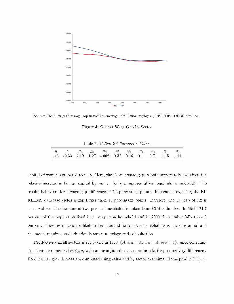
Source: Trends in gender wage gap in median earnings of full-time employees, 1980-2008 - OECD database
Figure 4: Gender Wage Gap by Sector
Table 2: Calibrated Parameter Values
η ε gi gs gn ψ ψs ai as γ σ.45 -2.33 2.12 1.27 -.002 0.32 0.46 0.11 0.71 1.15 4.44
capital of women compared to men. Here, the closing wage gap in both sectors takes as given the
relative increase in human capital by women (only a representative household is modeled). The
results below are for a wage gap di�erence of 7.2 percentage points. In some cases, using the EU
KLEMS database yields a gap larger than 15 percentage points, therefore, the US gap of 7.2 is
conservative. The fraction of two-person households is taken from CPS estimates. In 1960, 71.7
percent of the population lived in a two-person household and in 2000 the number falls to 55.3
percent. These estimates are likely a lower bound for 2000, since cohabitation is substantial and
the model requires no distinction between marriage and cohabitation.
Productivity in all sectors is set to one in 1960, {Ai1960 = As1960 = An1960 = 1}, since consump-
tion share parameters {ψ,ψs, ai, as} can be adjusted to account for relative productivity di�erences.
Productivity growth rates are computed using value add by sector over time. Home productivity gn
17

captures improvements in home technology over time. No good estimates exist on this growth rate
(see for example Ngai and Petrongolo, 2012; Rogerson, 2008). Rogerson (2008) uses gn = −.002
in a similar model. Since, this study is interested in capturing the interaction of taxes, structural
change and female employment, gn is set so as to match the rise in female employment. Results for
both growth rates are given below. The probability that women �nd service sector employment, γ,
is set to match the fraction of women in services in 2000. The probability of �nding a job is allowed
to vary with time, λt = γhi,tht
, consistent with the fact that the service sector is growing and should,
therefore, make it easier for women to �nd the most desirable job. The value for γ being close
to one implies that in 1960, 26 percent of women can only �nd employment in industry (however,
women can choose to work zero hours). In 2000, the share is 14 percent. While this friction might
seem large, it is in fact reasonable given the representative household structure. The remaining
preference parameters {ψ,ψs, as, ai, σ}, the weight on leisure of married and single households, the
relative taste for market services and industry goods, and the curvature on leisure are set in order
to match the following six 1960 and 2000 targets:
• Relative services hours in 1960 and 2000;
• Female market hours in 2000;
• Male market hours in 2000;
• Single female to married female market hours in 2000; and
• A Frisch elasticity of 0.5 for men in 2000.
The model is primarily calibrated to 2000, since hours worked data is not always available for 1960.
5.1 Results
The model does well in matching all targets, with home productivity of gn = −.002. Table 3
shows the US data targets with the model results. Only values labeled with ? were targeted in the
calibration. The Frisch elasticity of labor for males (not reported in the table) is matched perfectly
at 0.5 in 2000. The elasticity is 0.45 in 1960. For women the elasticities are 0.71 in 2000 and 1.03
18

in 1960. Micro estimates for male Frisch elasticities range from 0 to 0.5 for men and 0.5 to 2.2 for
women (for a survey on Frisch elasticities see Reichling and Whalen, 2012) putting the resulting
elasticities of the model within standard estimates.
The calibration underestimates the rise in female hours worked by 2.2 percentage points, and
the fall in male hours by 2.9 percentage points. It explains roughly 77 percent of the rise in female
hours observed in the US and 53 percent of the fall in men's hours. It over estimates married
women's relative market hours in 1960, this is partially due to the simpli�ed modeling of home
production and perfect complementarities in leisure for spouses, and the inability to match the
total rise in hours. In the model, men do no home production, while spouses' leisure are perfect
compliment. Without targeting total hours, the model does well in generating 54 percent of the
total rise observed in the data.
Table 3: US Targets
Hs/H H Hm Hf Hsf/H
mf Hsf/Hf
1960 Data 62.9 23.7 35.8 12.2a 3.2 77.4b
1960 Model 63.9? 25.7 33.0 14.5 1.9 79.0
2000 Data 75.6 26.0 30.4 21.6 1.2 86.92000 Model 73.8? 26.9 30.5? 21.6? 1.2? 86.9?
aHours in 1960 are estimated using employment rates in 1960 and ratio of hours to employment in 1968.bEU KLEMS 1968 value.
Previous research has shown the importance of home technology improvements in pushing women
into the labor market. Since, the paper aims to quantify the importance of structural change,
taxes, and gender wages on female employment and service sector employment, it is important to
match the total rise in female employment with the calibration. A home technology growth rate of
gn = −0.0072 does match the total rise in female employment from 1960 to 2000 in the US. Table 4
provides the estimates from table 3 above. The model now perfectly matches the magnitude of the
rise in total hours worked in the US, allowing for a precise comparison of higher taxes and di�erent
structural change. It also does slightly better in matching the rise in service employment.
19

Table 4: US Targets (Adjusted gn)
Hs/H H Hm Hf Hsf/H
mf Hsf/Hf
1960 Data 62.9 23.7 35.8 12.2 3.2 77.41960 Model 63.3? 24.6 32.8 12.3 2.4 78.7
2000 Data 75.6 26.9 30.4 21.6 1.2 86.92000 Model 74.9? 26.0 30.4? 21.6? 1.2? 86.9?
5.2 Counterfactuals
Counterfactuals to capture the importance of structural change, marketization, the feedback e�ect
of women entering the labor market in service employment, and the changing gender wage gap, are
provided. Table 5 provides estimates of changes in total hours, male hours, and female hours.
The �rst row provides the data equivalent. The second row restates the percentage point
changes from the benchmark model with gn = −0.0072.9 The �rst counterfactual assume only
taxes increased, i.e., gi = gs = gn = 0 and the wage gap remained at the initial 1960 level. This
counterfactual is simply to show the e�ect of the 2000 tax rate on 1960 working time. The second
counterfactual provides estimates for structural changes in the labor market over time. That is,
gs and gi are as-in the benchmark; the growth rate of home technology is set to the growth rate
of market services, gn = gs, to erase any e�ects from marketization of services; and the wage gap
remains at the 1960 level (taxes are set as-in table 1). The third counterfactual estimates structural
change, including marketization of services. Speci�cally, home technology grows at the benchmark
value. The fourth and �nal counterfactual estimates the e�ects of the closing gender wage gap,
while structural change is set to zero, gi = gs = gn = 0. If 2000 tax rates were present in the 1960
economy, total hours would be 127 percent lower, mostly driven by a fall, rather than a rise, in
female hours. Female hours are highly responsive to taxes, given their �exibility of choice in work-
ing at home when living in a two-person household. Single women's hours are rather unresponsive.
Structural change in the labor market without marketization also generates a fall in hours. Goods,
which are substitutable with services, become cheaper. Therefore, households' income goes further
9Appendix A provides, for comparison, the results with gn = −0.002.
20

Table 5: US Hours Counterfactual (Adjusted gn)
∆H ∆Hm ∆Hf
Data 2.3 -5.4 9.3
Benchmark 2.4 -2.4 9.3Explained (%) 102 48 100
2000 Taxes in 1960 -2.9 -2.7 -1.9Explained (%) -127 50 -20
Structural Change -3.7 -2.9 -2.6Explained (%) -161 53 -28
Structural Change and Marketization 0.1 -2.0 4.6Explained (%) 7 38 50
Gap 0.1 -3.1 4.3Explained (%) 2 58 47
in the market and market services can be produced at home instead. Allowing for marketization
and structural change can explain 50 percent of the rise in female hours, but only 7 percent of
the total hours worked di�erence. Similarly, the changing gender wage gap explains 47 percent of
changes in female hours worked, but again, hardly any of change in total hours worked.
Table 6 provides the decomposition of the change in service sector employment for the bench-
mark. These results provide insight into a number of interesting questions, such as: What has
driven the large increase in service employment? How much of the rise in service sector employment
can be explained by working women demanding more market services than stay-at-home women?
How large is the feedback e�ect discussed in the Introduction? This table decomposes the rise
in service sector employment by the portion driven by tax changes (recall taxes went up in all
regions), and the portion driven by women entering the labor force and, therefore, substituting
home for market services. The benchmark accounts for 91 percent of the rise in US service sector
Table 6: US Service Employment (Adjusted gn)
∆Hs/H Tax SC SC plus Home Women
Data 12.7
Benchmark 11.6 -0.6 -1.2 4.8 6.0Explained (%) 91 -4 -9 37 47
21

employment. Decomposing the rise shows that higher taxes decreased service sector employment
by 4 percent. Structural change (SC) in the labor market does not lead to an increase in female
employment and, therefore, the feedback mechanism in table 6 is absent. Including the relative fall
in home productivity, the decomposition for structural change and marketization explains roughly
37 percent. Relatively lower home productivity in the model incentivizes women to enter the labor
market and, therefore, to substitute home for market services. In total, the decomposition on labor
force participation of women shows that 47 percent of the rise in service sector employment, or 6
percentage points of the 11.6, is due to women entering the labor market and substituting home
produced services for market services. The 6 percent are computed assuming the relative share of
market services to home produced services does not change for households (the share in equation
11). There are a few e�ects here, while working women demand more market services, women
working within the service sector in 2000 demand on average 7.7 percent more market services than
women working in the industry sector. Consequently, as the industry sector shrinks, and women
are more likely to �nd work in the service sector, the demand for market services increases even if
women do not increase their intensive margin of work.
In conclusion, women entering the labor force increases service sector employment substantially.
In addition, both structural transformation and changing female wages can account for roughly half
of the increase in female hours. In terms of structural transformation, marketization is the driving
mechanism.
5.3 Germany
As it has been argued, taxes result in less hours worked. If the US were to have had German
tax rates in 2000, the service employment share would have been 1.40 percentage points lower, total
hours worked would have decreased by 4.6 percentage points, with male hours decreasing by an
additional 2.8 and female hours decreasing 6.2 percentage points (see table 7.). The drop is large
both for men and women. Nonetheless, since female employment still rises, 45 percent of the rise
in service employment is explained by the larger demand of market services of working women.
However, as Rogerson (2008) argues, Europe was several years behind the US in terms of produc-
22

Table 7: US Targets (German 2000 Tax)
Hs/H H Hm Hf
2000 Data 75.6 26.9 30.4 21.62000 Model 73.5 22.3 27.7 15.4
2000-1960 Data 12.7 2.3 -5.4 9.32000-1960 Benchmark 11.6 2.4 -2.4 9.32000-1960 Model 10.2 -2.2 -5.1 3.1
tivity levels in 1960. The e�ects of higher taxes and lower structural change on female employment
are studied by setting the initial productivity levels Ai,1960, As,1960, and An,1960 to match the relative
hours in the German service sector, the hours of men in 1960 and the hours of women. Moreover,
the growth rates for sectors are computed using changes in value add for Germany from 1960 to
2000, with annual growth rates of gi = 0.042, gs = 0.033. Home productivity is assumed to grow
as-in the US, at gn = 0.0133 or −0.0199 per annum slower than the service sector. All remaining
preferences parameters are as-in the US. Gender wage gaps are unchanged given the OECD median
wage gap evidence of �gure 4.
Table 8 summarizes the results. The model is unable to match the hours worked of men in 1960.
Table 8: German Targets
Hs/H H Hm Hf
1960 Data 40.2 28.8 35.1 18.9a
1960 Model 40.2? 29.3 31.5? 18.9?
2000 Data 67.0 19.8 21.8 17.82000 Model 50.8 25.6 27.2 19.7
aHours in 1960 are estimated using employment rates in 1960 and ratio of hours to employment in 1968.
However, the model is able to explain 40 percent of the rise in service employment, 41 percent of
the fall in total hours, 33 percent of the fall in male hours, and it only generates a very small rise
in female hours.10 If taxes would have remained at the 1960 level instead, table 9 would look as
10Hours from the data in 1960 are estimated using employment rates by gender in 1960 and the ratio of hoursto employment in 1968. Given the rough estimate of hours in 1960, the di�erence between the model and data isnegligible.
23

follows (see table 9). Under this tax assumption, the model now generates a small rise in hours
Table 9: German Targets (1960 Tax)
Hs/H H Hm Hf
2000 Data 67.0 19.8 21.8 17.82000 Model 52.3 30.8 30.5 25.7
worked comparable to the US, with 1.5 percentage points. Men's hours would only fall slightly by
1.0 percentage point and women's hours would increase 6.7 percentage points. In comparison, the
benchmark �gures of the US are a fall of 2.4 percentage points for male hours and a rise of 9.3
percentage points for women. In summary, taxes can account for the bulk of the di�erence in hours
worked between the US and Germany. Unlike, previous tax and hours studies, this is achieved with
a standard Frisch elasticity of labor.11 This follows from modeling a two-person households where
one spouse can stay home and the household bene�ts from specialization.
5.4 Sweden
Lastly, in comparing the tax policies of the US and Sweden we run a simple welfare experiment.
Preference parameters are as-in the US, since the focus here is simply on comparing the year 2000
and data from the 1960s is mostly missing for Sweden in these data sources. The benchmark model
is estimated using the tax rate of Sweden in 2000. Sweden has higher taxes, but provides large
subsidies, especially in the form of childcare, elderly care, etc. Since there is no good estimate of
the size of φ, the government subsidies tied to female employment, φ is set to match US working
hours in 2000. Two hypothetical �Swedish� economies are computed. First, all women have access
to the subsidy. Second, only married women have access to the subsidy, as the subsidy can be
dominated by childcare-related policies. The two computations provide a rough upper and lower
bound. One is to assume all women have children regardless of their relationship status (i.e., if they
have a partner or not). The other is to assume that only women with a partner have children and
access to the subsidy. The resulting subsidies are φ = 0.3531 if all women bene�t and φ = 0.603 if
11Olovsson (2009) also generates hours di�erences between the US and Sweden with a Frisch elasticity of 0.5.However, he does not explicitly model or study women's labor market choices.
24

only married women bene�t, which correspond to 14 percent and 29 percent of all market services
consumed, respectively. If only married women have access to the subsidy, the subsidy needs to
be larger in order to generate the same female hours. In general, the higher tax-subsidy scheme,
generates similar relative service hours of 74.7 compared to 74.9 in the benchmark. Men, however,
only work 26.70 percent of their time, and total hours are 25.02. This matches well with Swedish
data, where total hours worked was 23.5 in 2000. Hours of men are 29.5, slightly lower than in the
US.
Table 10 summarizes the main welfare results. Welfare is computed as follows: we ask by how
much both market goods and market service consumption would have to increase in the hypothetical
�Swedish� economies to make individuals indi�erent between the benchmark of low taxes and high
taxes but subsidies. The distortions are sizable. If all women can bene�t from the scheme, single
Table 10: Welfare Costs
Married Single Male Single Female Average
All Women 6.3 17.1 -12.9 4.4Married Women 4.1 25.7 18.7 12.2
men pay the largest price. Single men have little bene�ts from the subsidy and simply pay higher
taxes to �nance the subsidy. The bene�t for men is a large service sector and, therefore, slightly
lower prices. Moreover, married households still pay a cost, since dual earners are hit by higher
taxes and only receive a small subsidy. Single women are the only bene�ciaries from the scheme.
Single women have to work regardless of taxes or subsidies. Consequently, a subsidy to hours worked
brings in extra income. In contrast, if only married women bene�t from the scheme, the higher tax
regime is costly for all individuals. Now the average welfare cost rises from 4.4 percent to 12.2
percent in terms of market goods and service consumption loss.
6 Conclusion
To summarize, this paper develops a theory that can explain both a rise in services and a rise
in female labor supply concurrently. The model is consistent with general trends in labor supply
25

(male and female). Moreover, the rise in female employment is a large contributor to the rise
in service employment. Structural change accounts for roughly half of the increase and female
employment generating more market service demand accounts for the other half. The model also
accounts well for di�erences between Germany and the US in the service sector labor share and
female employment over time. A high tax country will have a smaller service sector and lower
female employment by subduing marketization. A simple computation of the social welfare loss of
high taxes and subsidizing female labor force participation in Sweden, compared to an equivalent
outcome in female labor force participation with low taxes and no subsidies, shows a non-negligible
loss. However, while the rise in the service sector is important in explaining part of the rise in
female employment, a striking conclusion is that high taxes are the main cause in generating lower
market hours and lower female employment in Europe compared to the US.
26

References
Aguiar, M., and E. Hurst (2007): �Measuring Trends in Leisure: The Allocation of Time over
Five Decades,� The Quarterly Journal of Economics, 122(3), 969�1006.
Albanesi, S., and C. Olivetti (2006): �Gender Roles and Technological Progress,� 2006 Meeting
Papers 411, Society for Economic Dynamics.
Bick, A., and N. Fuchs-Schündeln (2012): �Taxation and Labor Supply of Married Women
across Countries: A Macroeconomic Analysis,� CEPR Discussion Papers 9115, C.E.P.R. Discus-
sion Papers.
Chang, Y., and F. Schorfheide (2003): �Labor shifts and economic �uctuations,� Working
Paper 03-07, Federal Reserve Bank of Richmond.
Duarte, M., and D. Restuccia (2010): �The Role of the Structural Transformation in Aggregate
Productivity,� The Quarterly Journal of Economics, 125(1), 129�173.
Fernandez, R. (2007): �Culture as Learning: The Evolution of Female Labour Force Participation
Over a Century,� CEPR Discussion Papers 6451, C.E.P.R. Discussion Papers.
Fogli, A., and L. Veldkamp (2007): �Nature or Nurture? Learning and Female Labour Force
Dynamics,� CEPR Discussion Papers 6324, C.E.P.R. Discussion Papers.
Goldin, C. D. (1990): Understanding the Gender Gap : An Economic History of American
Women. NBER Series on Long-term Factors in Economic Development.
Greenwood, J., A. Seshadri, and M. Yorukoglu (2002): �Engines of liberation,� Working
papers 1, Wisconsin Madison - Social Systems.
Ingram, B. F., and G. R. Neumann (2006): �The Returns to Skill,� Labour Economics, 13(1),
35�59.
Jones, L. E., R. E. Manuelli, and E. R. McGrattan (2003): �Why are married women
working so much?,� Sta� Report 317, Federal Reserve Bank of Minneapolis.
27

King, M., S. Ruggles, J. T. Alexander, S. Flood, K. Genadek, M. B. Schroeder,
B. Trampe, and R. Vick (2010): �Integrated Public Use Microdata Series, Current Population
Survey: Version 3.0. [Machine-readable database],� Minneapolis: University of Minnesota.
McDaniel, C. (2007): �Average Tax Rates on Consumption, Investment, Labor and Capital in
the OECD: 1950-2003,� Arizona state university mimeo.
(2010): �A cross country study of trends in time use,� Working paper.
Ngai, L. R., and C. A. Pissarides (2008): �Trends in Hours and Economic Growth,� Review of
Economic Dynamics, 11(2), 239�256.
Ngai, R., and B. Petrongolo (2012): �Structural Transformation, Marketization and Female
Employment,� Discussion paper.
Olivetti, C. (2006): �Changes in Women's Hours of Market Work: The Role of Returns to
Experience,� Review of Economic Dynamics, 9(4), 557�587.
Olovsson, C. (2009): �Why do Europeans Work so Little?,� International Economic Review,
50(1), 39�61.
Prescott, E. C. (2004): �Why do Americans work so much more than Europeans?,� Quarterly
Review, (Jul), 2�13.
Ragan, K. (2006): �Taxes, Transfers, and Time Use: Fiscal Policy in a Model with Household
Production,� University of chicago mimeo.
Reichling, F., and C. Whalen (2012): �Review of Estimates of the Frisch Elasticity of Labor
Supply,� Discussion paper.
Rendall, M. (2010): �Brain versus Brawn: the Realization of Women's Comparative Advantage,�
IEW - Working Papers 491, Institute for Empirical Research in Economics - IEW.
Rogerson, R. (2005): Women at Work: An Economic Perspectivechap. What Policy Should Do:
Comments, pp. 109�114. Oxford University Press, Oxford, edited by tito boeri, daniela del boca,
and christopher pissarides edn.
28

(2008): �Structural Transformation and the Deterioration of European Labor Market
Outcomes,� Journal of Political Economy, 116(2), 235�259.
Ruggles, S., J. T. Alexander, K. Genadek, R. Goeken, M. B. Schroeder, andM. Sobek
(2010): �Integrated Public Use Microdata Series: Version 5.0 [Machine-readable database],� Min-
neapolis: University of Minnesota.
Rupert, P., R. Rogerson, and R. Wright (1995): �Estimating Substitution Elasticities in
Household Production Models,� Economic Theory, 6(1), 179�93.
29

Appendix A
The following table provide the counterfactuals for the case with gn = −0.002. Since, this version
did well in matching most of the trends in hours. The results here are similar to table 5 and 5. That
is women's feedback e�ect can account for 44 percent of the rise in service employment compared
to 47 in the benchmark above. One marked di�erence is marketization has a much smaller e�ect on
Table 11: US Hours Counterfactual (gn = −0.002)
∆H ∆Hm ∆Hf
Data 2.3 -5.4 9.3
Baseline 1.2 -2.5 7.1Explained (%) 54 47 76
2000 Taxes in 1960 -2.9 -2.7 -2.0Explained (%) -127 49 -21
Structural Change -3.8 -2.8 -2.9Explained (%) -165 51 -31
Structural Change and Marketization -1.0 -2.2 2.4Explained (%) -42 40 26
Gap -0.2 -3.0 3.7Explained (%) -8 56 40
women's hours now. Only 26 percent of the total change compared to 50 percent in the benchmark
are explained. The e�ect of male hours is similar in both cases. In contrast, the gender wage gap
e�ect is only slightly smaller 40 percent to 47 percent.
30