The Sign-Definiteness Lemma and Its

Applications to Robust Transceiver

Optimization for Multiuser MIMO Systems

Ebrahim Avazkonandeh Gharavol and Erik G. Larsson

Linköping University Post Print

N.B.: When citing this work, cite the original article.

©2013 IEEE. Personal use of this material is permitted. However, permission to

reprint/republish this material for advertising or promotional purposes or for creating new

collective works for resale or redistribution to servers or lists, or to reuse any copyrighted

component of this work in other works must be obtained from the IEEE.

Ebrahim Avazkonandeh Gharavol and Erik G. Larsson, The Sign-Definiteness Lemma and Its

Applications to Robust Transceiver Optimization for Multiuser MIMO Systems, 2013, IEEE

Transactions on Signal Processing, (61), 2, 238-252.

http://dx.doi.org/10.1109/TSP.2012.2222379

Postprint available at: Linköping University Electronic Press

http://urn.kb.se/resolve?urn=urn:nbn:se:liu:diva-85874

1

The Sign-Definiteness Lemma and its

Applications to Robust Transceiver

Optimization for Multiuser MIMO SystemsEbrahim A. Gharavol and Erik G. Larsson

Division of Communication Systems, Electrical Engineering Department (ISY)

Linkoping University, 581 83 Linkoping, Sweden

Abstract

We formally generalize the sign-definiteness lemma to the case of complex-valued matrices and multiple

norm-bounded uncertainties. This lemma has found many applications in the study of the stability of control

systems, and in the design and optimization of robust transceivers in communications. We then present three

different novel applications of this lemma in the area of multi-user multiple-input multiple-output (MIMO) robust

transceiver optimization. Specifically, the scenarios of interest are: (i) robust linear beamforming in an interfering

adhoc network, (ii) robust design of a general relay network, including the two-way relay channel as a special

case, and (iii) a half-duplex one-way relay system with multiple relays. For these networks, we formulate the

design problems of minimizing the (sum) MSE of the symbol detection subject to different average power budget

constraints. We show that these design problems are non-convex (with bilinear or trilinear constraints) and semi-

infinite in multiple independent uncertainty matrix-valued variables. We propose a two-stage solution where in

the first step the semi-infinite constraints are converted tolinear matrix inequalities using the generalized sign-

definiteness lemma, and in the second step, we use an iterative algorithm based on alternating convex search

(ACS). Via simulations we evaluate the performance of the proposed scheme.

I. I NTRODUCTION

Robust design refers to a design problem in which there is some kind of uncertainty in the problem

data or parameters. In control engineering, this is a well-established discipline and there are many

standard texts on the subject, see, e.g., [1], [2] and the references therein. More recently, the robust

design paradigm has been used for various applications in signal processing and communications,

most notably antenna array beamforming problems. Some pioneering contributions for beamforming

Copyright (c) 2012 IEEE. Personal use of this material is permitted. However, permission to use this material for any other purposes

must be obtained from the IEEE by sending a request to pubs-permissions@ieee.org.

This paper describes work undertaken in the context of the LOLA project - Achieving LOw-LAtency in Wireless Communications

(www.ict-lola.eu). The research leading to these results has received funding from the European Community 7th SeventhFramework

Program under grant agreement No. 248993. E. Larsson is a Royal Swedish Academy of Sciences (KVA) Research Fellow supported by

a grant from the Knut and Alice Wallenberg Foundation. Partsof this paper were presented at the 49th Annual Allerton Conference 2011

[61], at the 45th Annual Asilomar Conference on Signals, Systems and Computers 2011 [62], and at the 4th IEEE International Workshop

on Computational Advances in Multi-Sensor Adaptive Processing (CAMSAP) 2011 [63].

March 7, 2013 DRAFT

2

applications are contained in [3], [4], which introduced the concept of robust beamforming, taking

uncertainties in the array response into account. Further fundamental contributions on robust beam-

forming can be found in, e.g., [5]–[13] (see also the references therein).

Many robust design problems can be cast as semi-infinite optimization problems (optimization

problems with infinitely many constraints). The sign-definiteness lemma which was first proposed by

I.A. Petersen [14] is a tool which reduces such a semi-infinite problem to a much simpler linear matrix

inequality. This lemma was motivated by the study of stability of systems with uncertain parameters

in control theory, and in that field it has also been used for robustH∞ control design. The lemma

is also applicable to the worst-case transceiver optimization designs considered in this paper (which

are completely different problems thanH∞ design). Hence, the lemma as such is extremely versatile

and useful in many different disciplines.

In this paper we generalize the sign-definiteness lemma to the case in which the system has

multiple uncertainties and all variables are complex valued. As we will see, this generalization has

many applications in joint robust transceiver optimization for multiuser multiple-input multiple-output

(MIMO) communication systems. We will present three specific applications: (i) an interfering adhoc

network, (ii) a general amplify-and-forward MIMO relay network (including two-way relaying as a

special case), and (iii) a multi-relay network. However, the applications of the lemma are not limited to

these three cases, and similar analysis and design strategies can be used for many related applications

as well. For example, it is possible to extend our method to “cognitive radio” setups that involve

additional constraints on the interference generated by the transmitters. The optimization variables in

the applications that we consider are the precoder and equalization filters. Specifically, we design a

set of linear precoders and equalizers, optimized under the assumption that only imperfect channel

state information (CSI) is available. We model the CSI uncertainty using a ball-shaped norm bounded

error (NBE) model and adopt a worst-case design methodology, resulting in a system design which

maximizes performance for the worst possible CSI realization as defined by the NBE. We also extend

the design problems to a cognitive radio (CR) setup. In this paper we use (sum) MSE to quantify

performance, see Section II for more details.

The application setups that we consider here represent goodmodels for many practically important

scenarios. For example, the interference channel represented by the interfering adhoc network appli-

cation is a common model for spectrum sharing in wireless networks [43]. The interference relay

channel represented by our general relay network model can model, for example the scenario of a

relay in a wireless system that is shared between multiple operators [45]. The two-way relay channel

using amplify-and-forward processing is known to be an important building block both for future

cellular and wireless sensor networks [44].

A. Related Recent Work

As already noted, robust optimization for beamforming applications has a significant history that

started with the pioneering work of [3] and was followed by several early, important papers [4],

[8], [10]. Later contributions to the topic include [5]–[7], [9], [11]–[13]. Next we will review the

March 7, 2013 DRAFT

3

most recent works which are related to our applications. Related problems have been considered

before for multiple-input single-output (MISO) and MIMO communication systems. For example

in [15]–[19] the transmitters for the MISO broadcast channel (BC) were optimized using different

design criteria including MSE, sum-MSE and signal-to-interference-plus-noise ratio (SINR) subject to

different power constraints in different setups includingCR networks. There are also many papers that

robustly design similar systems with multiple antennas at both ends (i.e., the MIMO case) [20]–[25]

in single-user or multi-user networks. All these problems are such that each semi-infinite constraint

includes only one uncertainty variable, and they mostly resort to the complex-valued version of the

sign-definiteness lemma published in [26] to resolve the semi-infiniteness of the constraints.

Similarly, there are several papers that study various aspects of the capacity and beamforming design

for relay channels, especially for the two-way relay channel (TWRC) [27]–[35] and the interference

relay channel (IRC) [36]–[42] with or without (CSI) uncertainty. In [36] the Gaussian IRC with

different relaying schemes like compress-and-forward, compute-and-forward, and hash-and-forward

is studied. The authors use a new approach to find an upper bound on the sum-rate capacity of such

a system, by studying the strong and the weak interference regimes and establish the sum-capacity,

which, in turn, serves as an upper bound on the sum-capacity of the Gaussian IRC with bounded relay

power. The capacity of a cognitive relay-assisted Gaussianinterference channel is studied in [37]. An

achievable rate region for the system is derived by combining the Han-Kobayashi coding scheme for

the general interference channel with dirty paper coding. Reference [37] also derives outer bounds on

the capacity region and obtains the number of degrees of freedom of the system. A novel sum-rate

outer bound for the Gaussian interference channel with a relay is presented in [38] and [39]. The power

allocation problem for interference relay channels is considered in [40], [41]. Due to the competitive

nature of the multiuser environment, the problem is modeledas a strategic non-cooperative game. It

is shown that this game always has a unique Nash equilibrium.A hash-and-forward relaying scheme

is studied in [42].

B. Contributions

This paper unifies the results presented in our conference papers [61]–[63] in a comprehensive form

and presents additional discussion and comparisons. The specific contributions of the paper are:

• We generalize the sign-definiteness lemma to the case of complex-valued quantities with multiple

uncertainties in each design constraint.

• We formulate and solve the linear beamforming problem in an interfering adhoc network. This

contribution generalizes the method employed in [25] in which the authors assumed that each

MSE constraint is only affected by one single uncertainty source.

• We propose a generalized model for a relaying network, whichincludes the cases of TWRC and

IRC with direct links, and we optimally design precoders andequalizers for this network.

• We show that the theory developed for the aforementioned networks can be applied to a multi-

relay network as well.

March 7, 2013 DRAFT

4

The philosophy of the presentation is to highlight the wide range of the applications of the sign-

definiteness lemma, and to illuminate the similarities in the design methods used for the different

network topologies. The structure of the remainder of this paper is as follows. System models and

problem formulations for robust beamforming in the interfering adhoc network, in the general relay

network, and in the multi-relay network are presented in Sections II-B, II-C and II-D, respectively.

In Section III we present the generalized version of the sign-definiteness lemma and prove it. The

robust solution to the previously introduced problems are given in Section IV. Simulation results are

provided in Section V. Section VI concludes the paper.

Notation: Boldfaced letters are used for vectors or matrices. The fieldof the complex numbers,

the field of n-dimensional complex vectors and the field ofm × n-dimensional complex-valued

matrices are denoted byC, Cn and Cm×n, respectively. For any vectorx or for any matrixX,

‖x‖ and‖X‖F denote the Euclidean and the Frobenius norms of that vector or matrix, respectively.

To denote the transpose and conjugate transpose of a matrix,(·)T and (·)∗ are used.ℜ{·} denotes

the real part of its argument. Positive semi-definiteness ofa matrix X is denoted byX � 0. To

show a vertically concatenated vectorized version of a matrix, we write vec [], and to show the block

diagonal concatenation of a set of matrices we writeblkdiag [. . . ], respectively. Finally,Ex [f(x)] is

the expectation off(x) with respect to the stochastic variablex.

II. SYSTEM MODEL AND PROBLEM FORMULATIONS

In this section we present the system models and problem formulations of the three different

applications. It should be noted that the application of thesign-definiteness lemma, which will be

presented in the next sub-sections is not limited to these three networks. This lemma can be applied

to any general robust mean-squared error estimation in the presence of model uncertainties (see, e.g.,

Section IV of [26]), especially when there are several independent uncertainties associated with each

design constraint.

We will use an MSE based problem formulation. The MSE is a wellestablished measure for the

type of problem we consider [15]–[17], [19]–[25], [27] and in general in the context of severely

delay constrained applications that use short codes or evenuncoded transmission, see for example

[54]–[56]. Note also that short inner codes optimized with respect to MSE may be used as building

blocks in communication systems that have an outer error-correcting code, in a similar spirit to the

way space-time block codes based on signal-space diversitytechniques can be used as inner codes in

coded multiantenna transmissions.1 Unfortunately, extending our framework to using achievable rate

instead of MSE does not appear to be directly possible, and wehave to leave this as an open problem.

It is also noteworthy that throughout this paper we assume that the receivers, where applicable, treat

the interference as noise and do not try to decode it first.

We will first give a brief background on the uncertainty and the model we use to describe it, and

then we will proceed with the applications.

1Strictly speaking, using mutual information as performance metric is better than MSE in this context, e.g., see [57].

March 7, 2013 DRAFT

5

+

+

+

......

......

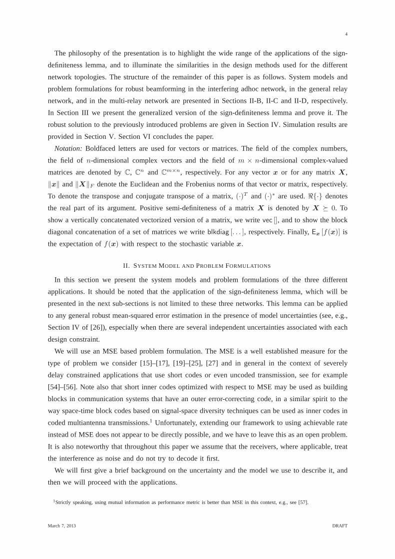
Fig. 1. Signal flow graph of an interfering adhoc network

A. Background

In the following examples, we assume that the model uncertainty is due to uncertainty in the

CSI. Since we are interested in MIMO communications, an uncertain CSI, sayH ∈ Cm×n can be

described using the following NBE model (see, e.g., [4] and the references therein):

H ∈ H , {H +∆ | ‖∆‖F ≤ δ}. (1)

In this notationH is the nominal value of the channel (that is known to the transmitter and receiver)

and∆ is the deterministically unknown perturbation term ofH. The only information that we have

regarding∆ is that it is norm bounded.

The motivation to use a spherical uncertainty region is twofold: (1) with Gaussian distributions, this

is the region with the smallest volume that contains a given probability mass. (2) Given knowledge

only of the error magnitude range but no other information about it, a spherical uncertainty region is

reasonable from a symmetry point of view.

In today’s communication systems, the receiver typically estimates the CSI using pilot symbols sent

from the transmitter side. The receiver usually sends this CSI back to the transmitter side. Because

of estimation errors, the CSI is generally uncertain, and owing to quantization errors the uncertainty

of the CSI at the transmitter could be different from the uncertainty of the CSI at the receiver. In this

paper, however, we use a single model to describe both uncertainties. This is simple, and moreover it

is natural if the design of both the transmitter and receiverfilters is done jointly at a central processing

node, and then both the transmitter and the receiver are informed of the matrices that they should

use. In this case, there is only nominal version of each channel, although the receivers could have

done somewhat better as they would typically have a higher quality CSI.

B. Application 1: Multiuser Interfering Network

1) System Model: The first application is transceiver optimization for an interfering adhoc network,

see Fig. 1. In this network,I independent links (Tx-Rx pairs) are communicating over a shared

channel. In theith link, i = 1, · · · , I; the Tx node aims to sendSi independent data streams using

March 7, 2013 DRAFT

6

Ti antennas towards the destination (Rx node) which is equipped with Ri receive antennas. We

assume that the symbols emitted by the source are zero-mean,independent and have equal energy,

i.e., Esi[si] = 0,Esi

[sis∗i ] = I, wheresi ∈ C

Si is the transmitted vector of the source node. This

information is linearly precoded using the precoding matrix P i ∈ CTi×Si and is sent towards the

destination over a Rayleigh fading wireless MIMO channelHii ∈ CRi×Ti . Each link also interferes

with the other links and the unintended receivers receive the transmitted signal over the channels

Hij ∈ CRj×Ti , j = 1, · · · , I, and j 6= i. In each Rx node, the received data is linearly equalized

using the receive matrixDi ∈ CSi×Ri . The received vector signal at the receiver is equal to

si = Di

H iiP isi +

I∑

j=1j 6=i

HjiP jsj + ni

(2)

whereni ∈ CRi is zero-mean white Gaussian noise with varianceσ2i .

Unlike in conventional design problems, in this paper, the CSI is not assumed to be perfectly

known. We use a NBE model framework [4] to describe the imperfect CSI. More precisely,Hij can

take on values as follows:

Hij ∈ Hij = {Hij +∆ij | ‖∆ij‖F ≤ δij}, (3)

whereHij is the nominal CSI and∆ij denotes the norm-bounded uncertainty. To best design this

network, we can jointly optimize the precoding and equalization matrices in different ways as will

be described in the following sections.

2) Worst-case Problem Formulation: In the problem formulations that we target in this paper, the

MSE of each link (MSEi,∀i) and the transmit power of each Tx node (TxPi,∀i) play important roles.

These quantities are defined as follows:

TxPi , Esi

[

‖P isi‖2]

,∀i, (4a)

MSEi , E{si}∀i

[

‖si − si‖2]

, ∀i, (4b)

= E{si}∀i

∥

∥

∥

∥

∥

∥

∥

∥

(DiHiiP i − ISi)si +

I∑

j=1j 6=i

DiHjiP jsj +Dini

∥

∥

∥

∥

∥

∥

∥

∥

2

, ∀i. (4c)

We will give the exact expressions for these quantities below. In the following problem formulations

we exploit the worst-case methodology, i.e., the constraints of the resulting optimization problems

should be satisfied for all possible channel realizations defined based on the NBE framework of (3),

including the least favorable one. It is clear that the leastfavorable (worst-case) channel realization

results in the largest MSE or transmit power.

One way to formulate the design problem for this network is tominimize the system-wide sum

MSE of the symbol detection subject to an average transmit power constraint for each link. This

March 7, 2013 DRAFT

7

optimization problem in its epigraph form can be written as follows:

minimize{P i,Di,τi≥0}I

i=1

I∑

i=1

τi (MIN-1)

subject to TxPi ≤ γi, ∀i,

MSEi ≤ τi, {∀Hij ∈ Hij}i,j,∀i.

whereγi is the power budget for theith link. An alternative way of formulating the problem is to

minimize the sum-transmit power, subject to MSE constraints (µi), as follows:

minimize{P i,Di,τi≥0}I

i=1

I∑

i=1

τi (MIN-2)

subject to TxPi ≤ τi, ∀i,

MSEi ≤ µi, {∀Hij ∈ Hij}i,j,∀i.

Although both these formulations are useful from the perspective of system design, none of them

will guarantee fairness among the different links. In the designs mentioned above, it is possible that

the link with the best CSI is allocated most of the available resources of the network, which leads

to poor service for the others. To prevent this unwanted event, we propose the following min-max

fairness formulation, in which the network is optimized to guarantee the best possible service for the

weakest link. This min-max fairness problem formulation for the MSE minimization can be written

as follows:

minimize{P i,Di}

max∀Hij∈Hij ,∀i,j

MSEi (MIN-3)

subject to TxPi ≤ γi.

which is equivalent to the following problem:

minimize{P i,Di}I

i=1,τ≥0τ (5a)

subject to TxPi ≤ γi, ∀i, (5b)

MSEi ≤ τ {∀Hij ∈ Hij}i,j,∀i. (5c)

It is clear that despite the different perspectives based onwhich the optimization problem is

formulated, the resulting optimization problems have a similar structure, and it suffices to give solution

details for one of them. By appropriately introducing slackvariables, a similar procedure can be

applied to other formulations.

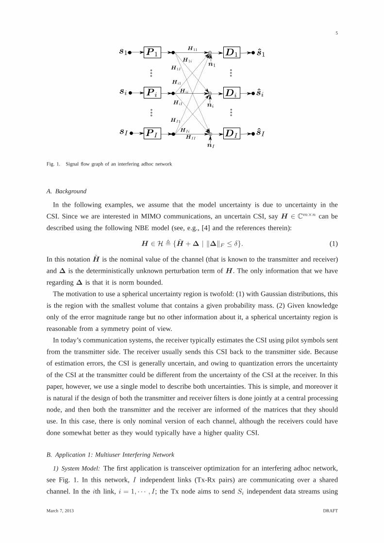
C. Application 2: General Non-Regenerative Amplify and Forward Interfering Relay Network

1) System Model: The signal flow diagram of a general wireless relay system is depicted in Fig. 2.

In this system, two distinct transmitter-receiver pairs simultaneously communicate with each other

in two consecutive time slots. Each pair has its own transmitand receive sides. Unlike the one-way

relay channel in which, to initiate a half-duplex communication service, two distinct time slots are

March 7, 2013 DRAFT

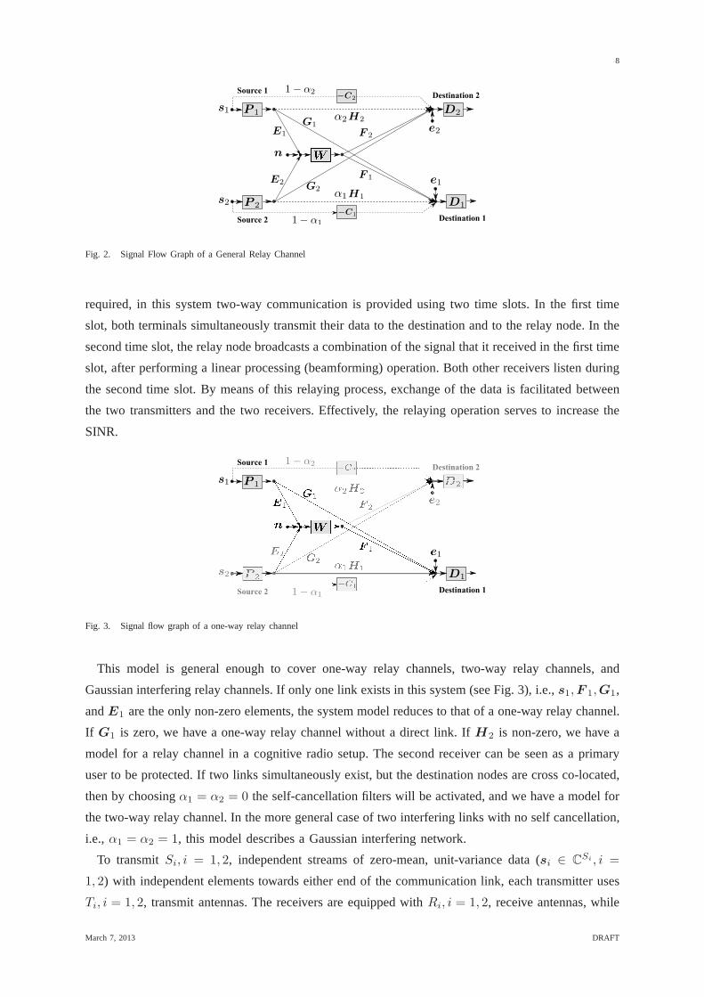
8

Source 1

Source 2 Destination 1

Destination 2

Fig. 2. Signal Flow Graph of a General Relay Channel

required, in this system two-way communication is providedusing two time slots. In the first time

slot, both terminals simultaneously transmit their data tothe destination and to the relay node. In the

second time slot, the relay node broadcasts a combination ofthe signal that it received in the first time

slot, after performing a linear processing (beamforming) operation. Both other receivers listen during

the second time slot. By means of this relaying process, exchange of the data is facilitated between

the two transmitters and the two receivers. Effectively, the relaying operation serves to increase the

SINR.

Source 1

Source 2 Destination 1

Destination 2

Fig. 3. Signal flow graph of a one-way relay channel

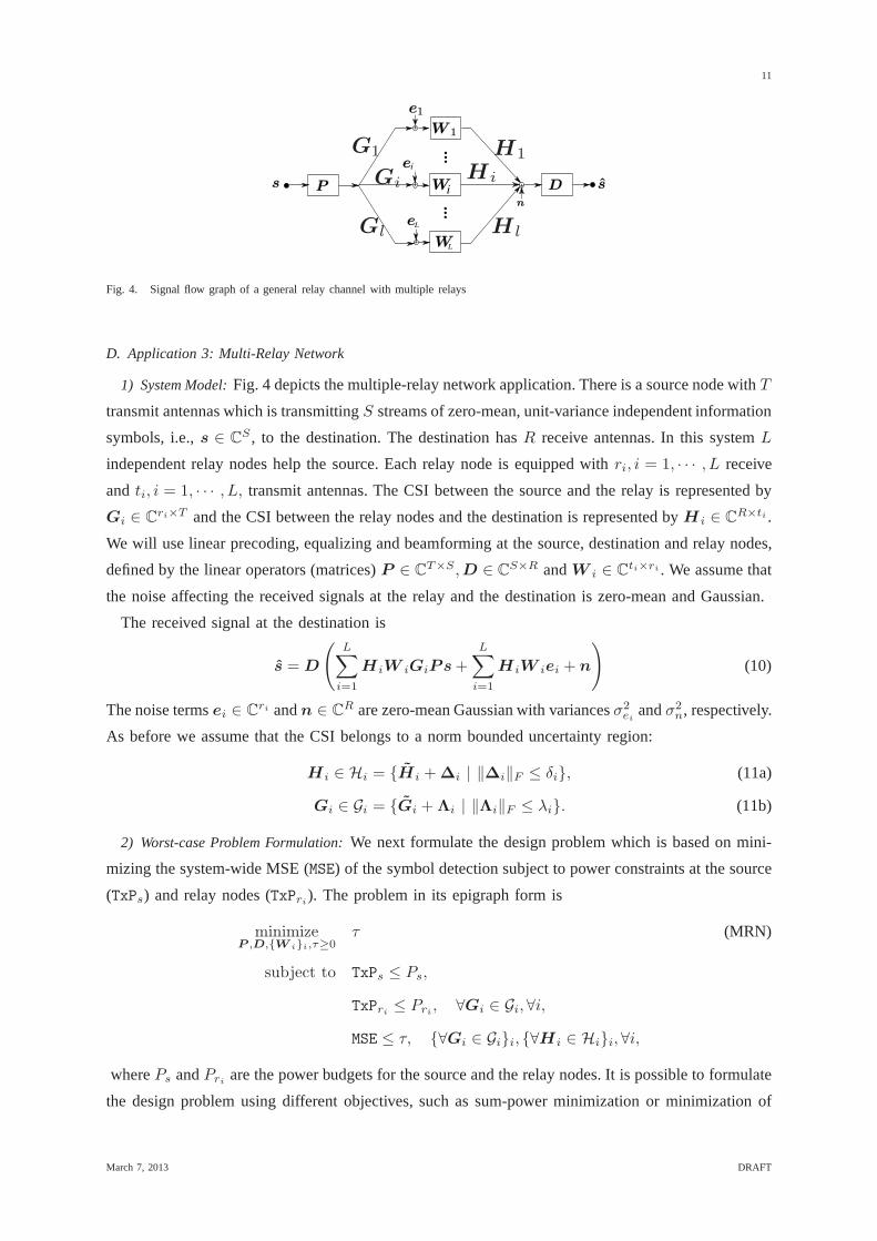
This model is general enough to cover one-way relay channels, two-way relay channels, and

Gaussian interfering relay channels. If only one link exists in this system (see Fig. 3), i.e.,s1,F 1,G1,

andE1 are the only non-zero elements, the system model reduces to that of a one-way relay channel.

If G1 is zero, we have a one-way relay channel without a direct link. If H2 is non-zero, we have a

model for a relay channel in a cognitive radio setup. The second receiver can be seen as a primary

user to be protected. If two links simultaneously exist, butthe destination nodes are cross co-located,

then by choosingα1 = α2 = 0 the self-cancellation filters will be activated, and we havea model for

the two-way relay channel. In the more general case of two interfering links with no self cancellation,

i.e., α1 = α2 = 1, this model describes a Gaussian interfering network.

To transmitSi, i = 1, 2, independent streams of zero-mean, unit-variance data (si ∈ CSi , i =

1, 2) with independent elements towards either end of the communication link, each transmitter uses

Ti, i = 1, 2, transmit antennas. The receivers are equipped withRi, i = 1, 2, receive antennas, while

March 7, 2013 DRAFT

9

the relay hasr andt receive and transmit antennas, respectively. The source nodes precode the data

using the precoding matricesP i ∈ CTi×Si . The precoded data is then sent over the wireless fading

channelsGi ∈ CRi×Ti ,H i ∈ C

Ri×T−i ,Ei ∈ Cr×Ti , i = 1, 2, whereX−i with the subscript−i

refers to a quantity belonging to the other index in the bi-index notation we use here. That is

X−i =

X2, i = 1,

X1, i = 2.(6)

At the relay node, the received signal is amplified usingW ∈ Ct×r. The resulting signal is transmitted

to the destinations in the next time slot over the channelsF i ∈ CRi×t, i = 1, 2.

In the case of a TWRC, we setα1 = α2 = 0, since each terminal knows its own transmitted

signal. Then, first a self-cancellation filter,−Ci ∈ CRi×S−i , is applied to the received signal. The

aim of this filter is to suppress each node’s own signal which has been retransmitted by the relay.

After appropriately combining the received signals and decoding using the linear equalizersDi ∈

CSi×Ri , i = 1, 2, the received signals are as follows:

si = Di(Gi + F iWEi)P isi +Di [(αiHi + F iWE−i)P−i − (1− αi)Ci] s−i

+DiF iWn+Diei. (7)

In this equationn ∈ Cr and ei ∈ C

Ri are additive zero-mean noise signals with independent

elements and variancesσ2u and σ2

ei, respectively. Due to the limited feedback between the nodes,

it is assumed that only the nominal value of the CSI is known tothe system and that the CSI

follows the norm bounded error model. That is, for any complex-valued matrix quantity such as

Ei,−i,F i,−i,Gi,−i,H i,−i, sayX, we have:

X ∈ SX = {X +∆X | ‖∆X‖F ≤ δX}, (8)

where X is the fixed nominal value of the CSI for each of the channels and ∆X is the norm-

bounded variation (uncertainty) around this nominal value. We next use this signal model to formulate

optimization problems.

2) Problem Formulation: Our goal is to jointly optimize the source precoders, the relay beamformer,

and the destination equalizers. To do so, we can formulate our design problem either in terms of

a min-max fairness, relay transmit power minimization, or system-wide sum-MSE (SMSE) mini-

mization. After choosing the performance measure of the system, we can consider the corresponding

optimization problem with the power budgets of both sourcesand the relay node, or the allowed MSE

of each link.

To facilitate the computation of the MSE of each link, and thetransmit powers of the sources and

the relay nodes, we use Lemma 2 presented in Section IV. Basedon this lemma, the MSE of the

links (MSEi, i = 1, 2), and the transmit powers of the source (TxPsi , i = 1, 2) and the relay (TxPr)

March 7, 2013 DRAFT

10

nodes are given as follows:

TxPsi , Esi

[

‖P isi‖22

]

, i = 1, 2 (9a)

= ‖P i‖2F , (9b)

TxPr , Es1,2,u

[

‖W (E1P 1s1 +E2P 2s2) +Wu‖22]

(9c)

= ‖WE1P 1‖2F + ‖WE2P 2‖

2F + σ2

u‖W ‖2F , (9d)

MSEi , Es1,2,u,e1,2

[

‖si − si‖2]

, i = 1, 2 (9e)

= ‖Di(Gi + F iWEi)P i − I‖2F + σ2u‖DiF iW ‖

2F

+ ‖Di [(αiHi + F iWE−i)P−i − (1− αi)Ci] ‖2F + σ2

ei‖Di‖2F (9f)

Using these quantities, the problem formulation in its epigraph form to minimize the SMSE is as

follows:

minimizeP i,W ,Di,Ci,τi≥0

τ1 + τ2 (AFIRN-1)

subject to TxPsi ≤ Psi , i = 1, 2,

TxPr ≤ Pr, ∀(Ei,E−i) ∈ SEi× SE−i

, i = 1, 2,

MSEi ≤ τi, ∀Ei ∈ SEi,E−i ∈ SE−i

,F i ∈ SF i,Gi ∈ SGi

,H i ∈ SHi, i = 1, 2,

wherePsi andPr are the power budgets of the source nodes and the relay node. The design problem

to minimize the transmit power of the relay, and the min-max fairness problem are as follows,

respectively:

minimizeP i,W ,Di,Ci,τ≥0

τ (AFIRN-2)

subject to TxPsi ≤ Psi , i = 1, 2,

TxPr ≤ τ, ∀Ei ∈ SEi,E−i ∈ SE−i

, i = 1, 2

MSEi ≤ γi, ∀Ei ∈ SEi,E−i ∈ SE−i

,F i ∈ SF i,Gi ∈ SGi

,Hi ∈ SHi, i = 1, 2,

and

minimizeP i,W ,Di,Ci,τ≥0

τ (AFIRN-3)

subject to TxPsi ≤ Psi , i = 1, 2,

TxPr ≤ Pr, ∀Ei ∈ SEi,E−i ∈ SE−i

, i = 1, 2,

MSEi ≤ τ, ∀Ei ∈ SEi,E−i ∈ SE−i

,F i ∈ SF i,Gi ∈ SGi

,H i ∈ SHi, i = 1, 2,

wherePsi andPr are the power limits of the source and the relay nodes, andγi, i = 1, 2 are the

MSE targets for each link. All these three variants of the design problem have a similar structure,

and the theory which underlies each of them can be applied to the other two. Therefore, in Section

IV we only give further details on the solution to the SMSE problem formulation.

March 7, 2013 DRAFT

11

...

+

+

+

+

...

i

L

i

L

G1

Gi

Gl

H1

H i

H l

Fig. 4. Signal flow graph of a general relay channel with multiple relays

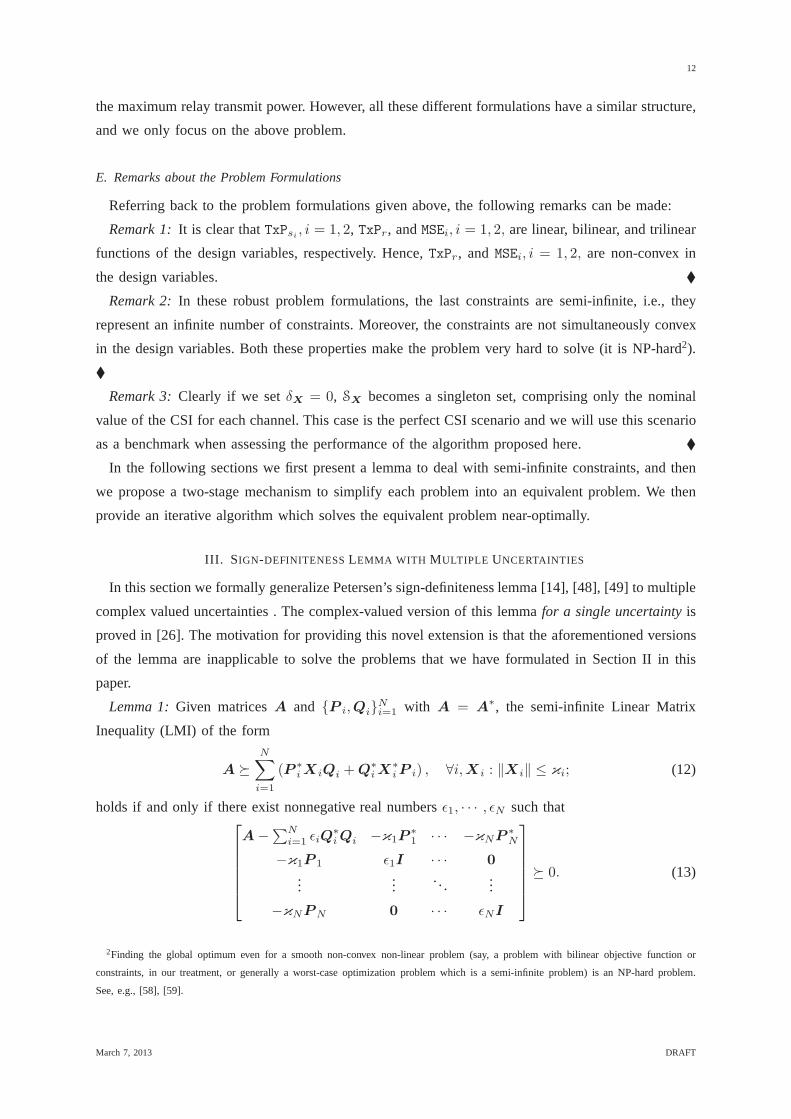
D. Application 3: Multi-Relay Network

1) System Model: Fig. 4 depicts the multiple-relay network application. There is a source node withT

transmit antennas which is transmittingS streams of zero-mean, unit-variance independent information

symbols, i.e.,s ∈ CS , to the destination. The destination hasR receive antennas. In this systemL

independent relay nodes help the source. Each relay node is equipped withri, i = 1, · · · , L receive

andti, i = 1, · · · , L, transmit antennas. The CSI between the source and the relay is represented by

Gi ∈ Cri×T and the CSI between the relay nodes and the destination is represented byH i ∈ CR×ti .

We will use linear precoding, equalizing and beamforming atthe source, destination and relay nodes,

defined by the linear operators (matrices)P ∈ CT×S,D ∈ CS×R andW i ∈ Cti×ri . We assume that

the noise affecting the received signals at the relay and thedestination is zero-mean and Gaussian.

The received signal at the destination is

s = D

(

L∑

i=1

HiW iGiPs+L∑

i=1

HiW iei + n

)

(10)

The noise termsei ∈ Cri andn ∈ C

R are zero-mean Gaussian with variancesσ2ei andσ2

n, respectively.

As before we assume that the CSI belongs to a norm bounded uncertainty region:

Hi ∈ Hi = {Hi +∆i | ‖∆i‖F ≤ δi}, (11a)

Gi ∈ Gi = {Gi +Λi | ‖Λi‖F ≤ λi}. (11b)

2) Worst-case Problem Formulation: We next formulate the design problem which is based on mini-

mizing the system-wide MSE (MSE) of the symbol detection subject to power constraints at thesource

(TxPs) and relay nodes (TxPri). The problem in its epigraph form is

minimizeP ,D,{W i}i,τ≥0

τ (MRN)

subject to TxPs ≤ Ps,

TxPri ≤ Pri , ∀Gi ∈ Gi,∀i,

MSE ≤ τ, {∀Gi ∈ Gi}i, {∀Hi ∈ Hi}i,∀i,

wherePs andPri are the power budgets for the source and the relay nodes. It ispossible to formulate

the design problem using different objectives, such as sum-power minimization or minimization of

March 7, 2013 DRAFT

12

the maximum relay transmit power. However, all these different formulations have a similar structure,

and we only focus on the above problem.

E. Remarks about the Problem Formulations

Referring back to the problem formulations given above, thefollowing remarks can be made:

Remark 1: It is clear thatTxPsi , i = 1, 2, TxPr, andMSEi, i = 1, 2, are linear, bilinear, and trilinear

functions of the design variables, respectively. Hence,TxPr, andMSEi, i = 1, 2, are non-convex in

the design variables. �

Remark 2: In these robust problem formulations, the last constraintsare semi-infinite, i.e., they

represent an infinite number of constraints. Moreover, the constraints are not simultaneously convex

in the design variables. Both these properties make the problem very hard to solve (it is NP-hard2).

�

Remark 3: Clearly if we setδX = 0, SX becomes a singleton set, comprising only the nominal

value of the CSI for each channel. This case is the perfect CSIscenario and we will use this scenario

as a benchmark when assessing the performance of the algorithm proposed here. �

In the following sections we first present a lemma to deal withsemi-infinite constraints, and then

we propose a two-stage mechanism to simplify each problem into an equivalent problem. We then

provide an iterative algorithm which solves the equivalentproblem near-optimally.

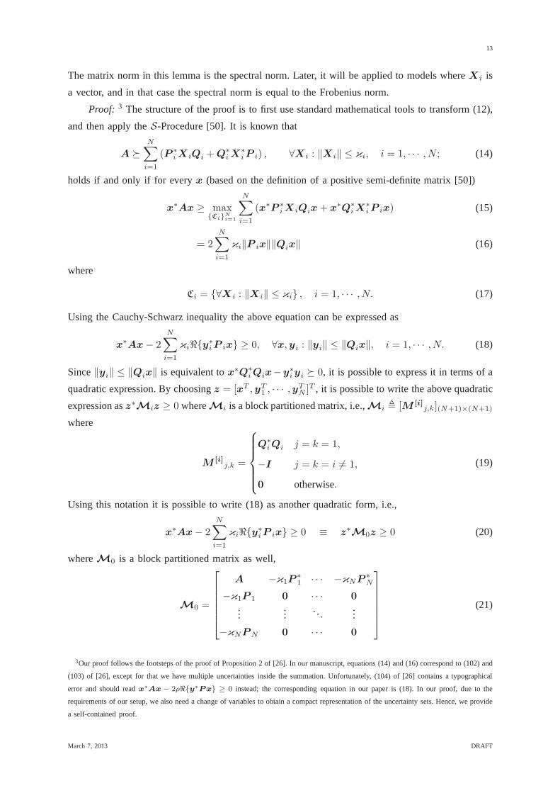
III. S IGN-DEFINITENESSLEMMA WITH MULTIPLE UNCERTAINTIES

In this section we formally generalize Petersen’s sign-definiteness lemma [14], [48], [49] to multiple

complex valued uncertainties . The complex-valued versionof this lemmafor a single uncertainty is

proved in [26]. The motivation for providing this novel extension is that the aforementioned versions

of the lemma are inapplicable to solve the problems that we have formulated in Section II in this

paper.

Lemma 1: Given matricesA and {P i,Qi}Ni=1 with A = A∗, the semi-infinite Linear Matrix

Inequality (LMI) of the form

A �

N∑

i=1

(P ∗iXiQi +Q∗

iX∗iP i) , ∀i,Xi : ‖Xi‖ ≤ κi; (12)

holds if and only if there exist nonnegative real numbersǫ1, · · · , ǫN such that

A−∑N

i=1 ǫiQ∗iQi −κ1P

∗1 · · · −κNP ∗

N

−κ1P 1 ǫ1I · · · 0

......

. . ....

−κNPN 0 · · · ǫNI

� 0. (13)

2Finding the global optimum even for a smooth non-convex non-linear problem (say, a problem with bilinear objective function or

constraints, in our treatment, or generally a worst-case optimization problem which is a semi-infinite problem) is an NP-hard problem.

See, e.g., [58], [59].

March 7, 2013 DRAFT

13

The matrix norm in this lemma is the spectral norm. Later, it will be applied to models whereXi is

a vector, and in that case the spectral norm is equal to the Frobenius norm.

Proof: 3 The structure of the proof is to first use standard mathematical tools to transform (12),

and then apply theS-Procedure [50]. It is known that

A �N∑

i=1

(P ∗iXiQi +Q∗

iX∗iP i) , ∀Xi : ‖Xi‖ ≤ κi, i = 1, · · · ,N ; (14)

holds if and only if for everyx (based on the definition of a positive semi-definite matrix [50])

x∗Ax ≥ max{Ci}N

i=1

N∑

i=1

(x∗P ∗iXiQix+ x∗Q∗

iX∗iP ix) (15)

= 2N∑

i=1

κi‖P ix‖‖Qix‖ (16)

where

Ci = {∀Xi : ‖Xi‖ ≤ κi} , i = 1, · · · ,N. (17)

Using the Cauchy-Schwarz inequality the above equation canbe expressed as

x∗Ax− 2N∑

i=1

κiℜ{y∗iP ix} ≥ 0, ∀x,yi : ‖yi‖ ≤ ‖Qix‖, i = 1, · · · ,N. (18)

Since‖yi‖ ≤ ‖Qix‖ is equivalent tox∗Q∗iQix−y∗

iyi � 0, it is possible to express it in terms of a

quadratic expression. By choosingz = [xT ,yT1 , · · · ,y

TN ]T , it is possible to write the above quadratic

expression asz∗Miz ≥ 0 whereMi is a block partitioned matrix, i.e.,Mi , [M [i]j,k](N+1)×(N+1)

where

M [i]j,k =

Q∗iQi j = k = 1,

−I j = k = i 6= 1,

0 otherwise.

(19)

Using this notation it is possible to write (18) as another quadratic form, i.e.,

x∗Ax− 2N∑

i=1

κiℜ{y∗iP ix} ≥ 0 ≡ z∗

M0z ≥ 0 (20)

whereM0 is a block partitioned matrix as well,

M0 =

A −κ1P∗1 · · · −κNP ∗

N

−κ1P 1 0 · · · 0

......

. . ....

−κNPN 0 · · · 0

(21)

3Our proof follows the footsteps of the proof of Proposition 2of [26]. In our manuscript, equations (14) and (16) correspond to (102) and

(103) of [26], except for that we have multiple uncertainties inside the summation. Unfortunately, (104) of [26] contains a typographical

error and should readx∗Ax − 2ρℜ{y∗Px} ≥ 0 instead; the corresponding equation in our paper is (18). Inour proof, due to the

requirements of our setup, we also need a change of variablesto obtain a compact representation of the uncertainty sets.Hence, we provide

a self-contained proof.

March 7, 2013 DRAFT

14

Using this notation, it is possible to reformulate (18) as the following implication:

z∗Miz ≥ 0, i = 1, · · · ,N ⇒ z∗

M0z ≥ 0 (22)

Using the general form of theS-procedure [50] for quadratic functions and non-strict inequalities,

(22) holds if there existsǫ1, · · · , ǫN ≥ 0 such that the LMI (13) holds and this completes the proof.

IV. ROBUST SOLUTION

In this section we will present the robust solution to the problem formulations for the three different

applications.

A. Preliminaries

Generally we use a two step solution. In the first step, we use the sign-definiteness lemma to convert

the semi-infinite problem to a biconvex approximate versionof that problem, and in the second step,

we use an iterative algorithm to deal with the bi-convexity of that approximate problem. We first

present a handy lemma which is helpful in formulating the performance measures, and then we give

the solutions.

Lemma 2: For any set of zero-mean, independent and identically distributed random vectors with

independent elements and individual covariances matricesExi[xix

∗i ] = σ2

i I we have

E{xi}i

∥

∥

∥

∥

∥

∑

i

Aixi

∥

∥

∥

∥

∥

2

2

=∑

i

σ2i ‖Ai‖

2F (23)

Proof: It is clear that

E{xi}i

∥

∥

∥

∥

∥

∑

i

Aixi

∥

∥

∥

∥

∥

2

2

=∑

i

∑

j

Exi,xj[x∗

iA∗iAjxj ]

=∑

i

∑

j

Exi,xj[tr [A∗

iAjxjx∗i ]]

=∑

i

∑

j

tr[

A∗iAjExi,xj

[xjx∗i ]]

=∑

i

σ2i tr [A

∗iAi] (24)

which proves the lemma.

B. Robust Solution to Application 1

Using Lemma 2,MSEi andTxPi can be written:

TxPi = ‖P i‖2F , ∀i, (25a)

MSEi = ‖DiHiiP i − ISi‖2F +

I∑

j=1j 6=i

‖DiHjiPj‖2F + σ2

ni‖Di‖

2F , ∀i. (25b)

March 7, 2013 DRAFT

15

Note that the MSE terms are norm-squared of matrix expressions that are bilinear in the design

variables. Hence, the MSE constraints are not only semi-infinite with orderI, but also non-convex.

This is what makes the aforementioned problems hard to solve. Stressing on this observation, we

outline our solution methodology as follows:

1) We first show thatMSEi can be represented as the norm-squared of a vector which is affine in

the channel uncertainties. Then using Lemma 1, we find an equivalent SDP formulation for the

problem at hand.

2) We then resort to an iterative algorithm based on the Alternating Convex Search (ACS) algorithm

[52], to overcome the non-convexity of the problem.

In the following we will describe these steps in more detail.

1) Step 1: Using the identity‖X‖F = ‖vec [X] ‖2 for any given matrixX, we can rewriteMSEi

as the norm-squared of a vector:

MSEi = ‖mi‖22 (26)

where

mi ,

vec [DiH1iP 1]...

vec [DiHIiP I ]

σ2nivec [Di]

− ii ∈ CSi(

∑Ij=1

Sj+Ri), (27)

and

ii =

0Si

∑i−1j=1 Sj×1

vec [ISi]

0Si(∑

Ij=i+1

Sj+Ri)×1

. (28)

Using the identityvec [ABC] = (CT ⊗ A)vec [B] for matrices of compatible dimensions, it is

possible to rewritemi as an affine combination of uncertainty terms:

mi = mi +I∑

j=1

M ij vec [∆ji], (29)

where

mi =

vec[

DiH1iP 1

]

...

vec[

DiHIiP I

]

σ2nivec [Di]

− ii ∈ CSi(

∑Ij=1

Sj+Ri) (30a)

and

M ij =

0(Si

∑j−1

k=1Sk)×RiTi

P Tj ⊗Di

0(Si(∑

Ik=j+1

Sk+Ri))×RiTi

. (31)

March 7, 2013 DRAFT

16

We next use the Schur Complement Lemma [50] to recast the MSE constraint as a matrix inequality,

and then we exploit the structure devised above together with Lemma 1. We know that the MSE

constraint, i.e.,‖mi‖22 ≤ τi, can be represented in terms of the following LMI4

[

τi m∗i

mi I

]

� 0, (32)

By inserting the structure of the MSE into the above equationwe have

τi m∗i

mi ISi(Ri+∑

Ij=1

Sj)

� −I∑

j=1

0 (M ijvec [∆ji])∗

M ijvec [∆ji] 0Si(∑

Ij=1

Sj+Ri)

. (33)

By appropriately choosing the the parameters of the sign-definiteness lemma as follows,

Ai =

τi m∗i

mi ISi(Ri+∑

Ij=1

Sj)

, (34a)

Qij =[

−1 01×(Si(Ri+∑

Ij=1

Sj))

]

, (34b)

P ij =[

0RiTj×1 M∗ij

]

, (34c)

we can recast theMSEi constraint as the following matrix inequality:

Ai −∑I

j=1 ǫijQ∗ijQij −δi1P

∗i1 · · · −δiIP

∗iI

−δi1P i1 ǫi1I · · · 0

......

. . ....

−δiIP iI 0 · · · ǫiII

� 0. (35a)

Note that the non-negativity of the slack variables follow from the preceding LMI. By assembling

all components, the sum-MSE minimization problem can now bewritten:

minimize{P i,Di,τi≥0,ǫij}I

i,j=1

I∑

i=1

τi (36a)

subject to TxPi ≤ γi, ∀i, (36b)

(35a) holds, ∀i (36c)

This problem is not semi-infinite anymore, but it is biconvex(due to the underlying structure ofAi

andP ij). Next we propose an iterative algorithm based on the ACS algorithm to solve it numerically.

2) Step 2: In what follows, we minimize the sum-MSE by first fixing a subset of the variables so

that the problem at hand reduces to a convex one in the remaining variables (including the slack

variables). We use interior point methods to solve the resulting convex problem. We then fix the

remaining subset of variables and do the same thing to updatethe first subset of variables. This

process continues until the desired accuracy is reached or until a certain number of iterations has

been carried out. The algorithm is summarized as follows:

4The robust version of a SOCP is generally an SDP (which means the complexity class of a robust problem is increased relative to the

original non-robust problem), see [60] and the references therein. The LMI-based formulation appears to be the most appropriate SDP,

because it is convex, and unlike the vector/matrix lifting process [51] which usually needs the non-convex rank-1 constraint relaxation, the

LMI-based formulation does not need any further assumptions or processing.

March 7, 2013 DRAFT

17

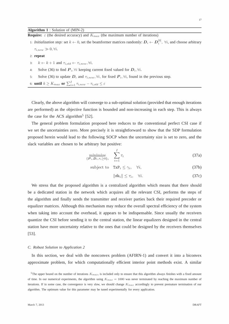
Algorithm 1 : Solution of (MIN-2)Require: ε (the desired accuracy) andKmax (the maximum number of iterations)

1: Initialization step: setk ← 0, set the beamformer matrices randomly:Di ←D[0]i , ∀i, and choose arbitrary

τi,new ≫ 0, ∀i.

2: repeat

3: k ← k + 1 andτi,old ← τi,new , ∀i.

4: Solve (36) to findP i, ∀i keeping current fixed valued forDi, ∀i.

5: Solve (36) to updateDi andτi,new, ∀i, for fixed P i, ∀i, found in the previous step.

6: until k ≥ Kmax or∑I

i=1 τi,new − τi,old ≤ ε

Clearly, the above algorithm will converge to a sub-optimalsolution (provided that enough iterations

are performed) as the objective function is bounded and non-increasing in each step. This is always

the case for the ACS algorithm5 [52].

The general problem formulation proposed here reduces to the conventional perfect CSI case if

we set the uncertainties zero. More precisely it is straightforward to show that the SDP formulation

proposed herein would lead to the following SOCP when the uncertainty size is set to zero, and the

slack variables are chosen to be arbitrary but positive:

minimize{P i,Di,τi≥0}i

I∑

i=1

τi (37a)

subject to TxPi ≤ γi, ∀i, (37b)

‖mi‖ ≤ τi, ∀i. (37c)

We stress that the proposed algorithm is a centralized algorithm which means that there should

be a dedicated station in the network which acquires all the relevant CSI, performs the steps of

the algorithm and finally sends the transmitter and receiverparties back their required precoder or

equalizer matrices. Although this mechanism may reduce theoverall spectral efficiency of the system

when taking into account the overhead, it appears to be indispensable. Since usually the receivers

quantize the CSI before sending it to the central station, the linear equalizers designed in the central

station have more uncertainty relative to the ones that could be designed by the receivers themselves

[53].

C. Robust Solution to Application 2

In this section, we deal with the nonconvex problem (AFIRN-1) and convert it into a biconvex

approximate problem, for which computationally efficient interior point methods exist. A similar

5The upper bound on the number of iterationsKmax, is included only to ensure that this algorithm always finishes with a fixed amount

of time. In our numerical experiments, the algorithm usingKmax = 1000 was never terminated by reaching the maximum number of

iterations. If in some case, the convergence is very slow, weshould changeKmax accordingly to prevent premature termination of our

algorithm. The optimum value for this parameter may be tunedexperimentally for every application.

March 7, 2013 DRAFT

18

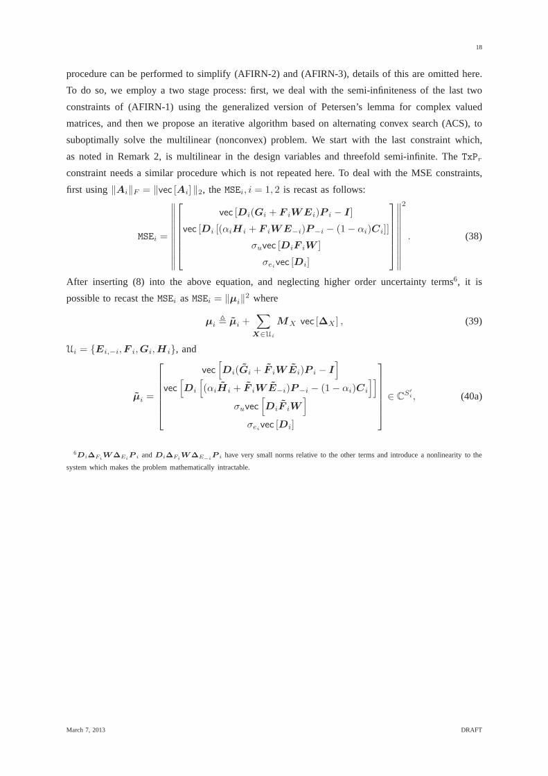
procedure can be performed to simplify (AFIRN-2) and (AFIRN-3), details of this are omitted here.

To do so, we employ a two stage process: first, we deal with the semi-infiniteness of the last two

constraints of (AFIRN-1) using the generalized version of Petersen’s lemma for complex valued

matrices, and then we propose an iterative algorithm based on alternating convex search (ACS), to

suboptimally solve the multilinear (nonconvex) problem. We start with the last constraint which,

as noted in Remark 2, is multilinear in the design variables and threefold semi-infinite. TheTxPr

constraint needs a similar procedure which is not repeated here. To deal with the MSE constraints,

first using‖Ai‖F = ‖vec [Ai] ‖2, the MSEi, i = 1, 2 is recast as follows:

MSEi =

∥

∥

∥

∥

∥

∥

∥

∥

∥

∥

∥

vec [Di(Gi + F iWEi)P i − I]

vec [Di [(αiHi + F iWE−i)P−i − (1− αi)Ci]]

σuvec [DiF iW ]

σeivec [Di]

∥

∥

∥

∥

∥

∥

∥

∥

∥

∥

∥

2

. (38)

After inserting (8) into the above equation, and neglectinghigher order uncertainty terms6, it is

possible to recast theMSEi asMSEi = ‖µi‖2 where

µi , µi +∑

X∈Ui

MX vec [∆X ] , (39)

Ui = {Ei,−i,F i,Gi,H i}, and

µi =

vec[

Di(Gi + F iWEi)P i − I]

vec[

Di

[

(αiHi + F iWE−i)P−i − (1− αi)Ci

]]

σuvec[

DiF iW]

σeivec [Di]

∈ CS′

i , (40a)

6Di∆FiW∆Ei

P i andDi∆FiW∆E−i

P i have very small norms relative to the other terms and introduce a nonlinearity to the

system which makes the problem mathematically intractable.

March 7, 2013 DRAFT

19

and subsequently

MGi=

[

P Ti ⊗Di

0

]

∈ Cm′

i×RiTi , (40b)

MEi=

[

P Ti ⊗DiF iW

0

]

∈ Cm′

i×rTi , (40c)

MHi=

0

αiPT−i ⊗Di

0

∈ Cm′

i×RiT−i , (40d)

ME−i=

0

P T−i ⊗DiF iW

0

∈ Cm′

i×rT−i , (40e)

MFi=

(WEiP i)T ⊗Di

(WE−iP−i)T ⊗Di

σuWT ⊗Di

0

∈ Cm′

i×Rit, (40f)

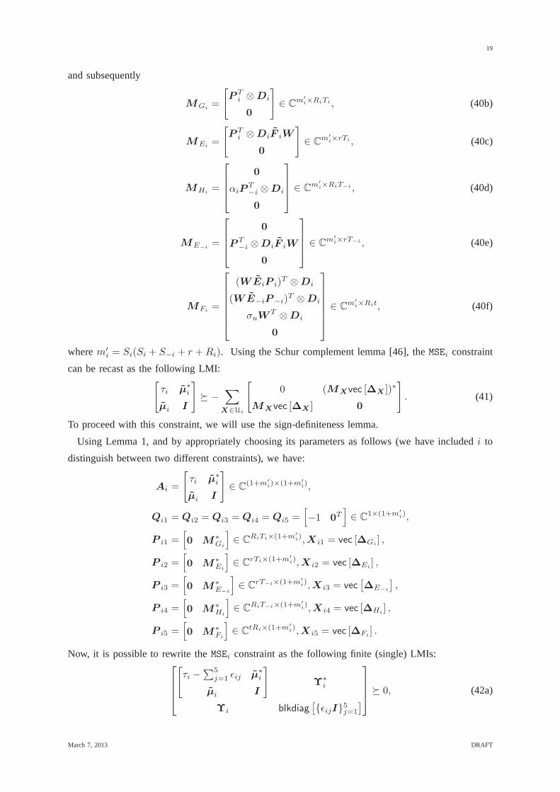
wherem′i = Si(Si + S−i + r + Ri). Using the Schur complement lemma [46], theMSEi constraint

can be recast as the following LMI:[

τi µ∗i

µi I

]

� −∑

X∈Ui

[

0 (MXvec [∆X ])∗

MXvec [∆X ] 0

]

. (41)

To proceed with this constraint, we will use the sign-definiteness lemma.

Using Lemma 1, and by appropriately choosing its parametersas follows (we have includedi to

distinguish between two different constraints), we have:

Ai =

[

τi µ∗i

µi I

]

∈ C(1+m′

i)×(1+m′

i),

Qi1 = Qi2 = Qi3 = Qi4 = Qi5 =[

−1 0T]

∈ C1×(1+m′

i),

P i1 =[

0 M∗Gi

]

∈ CRiTi×(1+m′

i),Xi1 = vec [∆Gi] ,

P i2 =[

0 M∗Ei

]

∈ CrTi×(1+m′

i),Xi2 = vec [∆Ei] ,

P i3 =[

0 M∗E−i

]

∈ CrT−i×(1+m′

i),Xi3 = vec[

∆E−i

]

,

P i4 =[

0 M∗Hi

]

∈ CRiT−i×(1+m′

i),Xi4 = vec [∆Hi] ,

P i5 =[

0 M∗Fi

]

∈ CtRi×(1+m′

i),Xi5 = vec [∆Fi] .

Now, it is possible to rewrite theMSEi constraint as the following finite (single) LMIs:

[

τi −∑5

j=1 ǫij µ∗i

µi I

]

Υ∗i

Υi blkdiag[

{ǫijI}5j=1

]

� 0, (42a)

March 7, 2013 DRAFT

20

where

Υi = −[δGiP T

i1 δEiP T

i2 δE−iP T

i3 δHiP T

i4 δF iP T

i5]T . (42b)

In this formulation, the non-negativity of the slack variables is automatically guaranteed, because the

LMI in (42a) requires that the diagonal elements of the matrix on the left-hand side are positive.

Henceτi also should be greater than or equal to the sum ofǫij which itself is the sum of positive

real numbers.

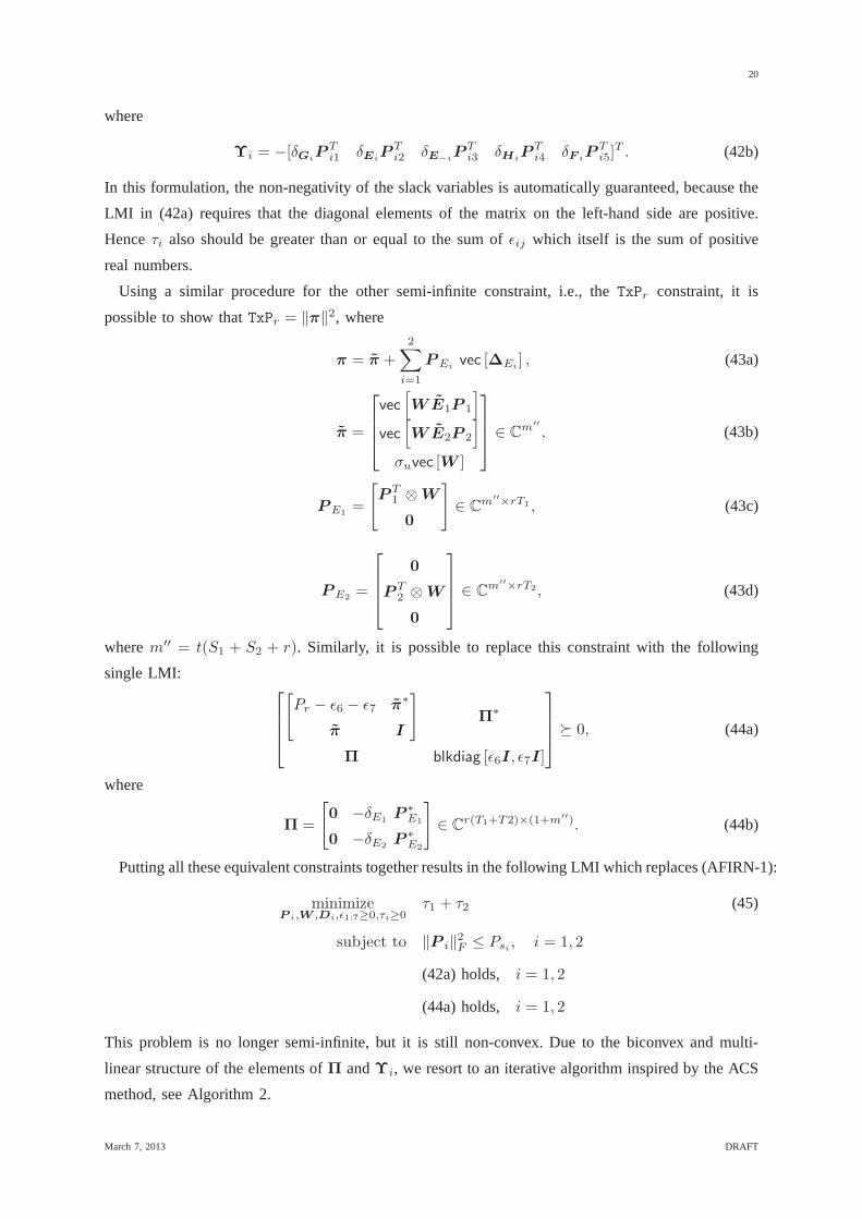
Using a similar procedure for the other semi-infinite constraint, i.e., theTxPr constraint, it is

possible to show thatTxPr = ‖π‖2, where

π = π +2∑

i=1

PEivec [∆Ei

] , (43a)

π =

vec[

WE1P 1

]

vec[

WE2P 2

]

σuvec [W ]

∈ Cm′′

, (43b)

PE1=

[

P T1 ⊗W

0

]

∈ Cm′′×rT1 , (43c)

PE2=

0

P T2 ⊗W

0

∈ Cm′′×rT2 , (43d)

wherem′′ = t(S1 + S2 + r). Similarly, it is possible to replace this constraint with the following

single LMI:

[

Pr − ǫ6 − ǫ7 π∗

π I

]

Π∗

Π blkdiag [ǫ6I, ǫ7I]

� 0, (44a)

where

Π =

[

0 −δE1P ∗

E1

0 −δE2P ∗

E2

]

∈ Cr(T1+T2)×(1+m′′). (44b)

Putting all these equivalent constraints together resultsin the following LMI which replaces (AFIRN-1):

minimizeP i,W ,Di,ǫ1:7≥0,τi≥0

τ1 + τ2 (45)

subject to ‖P i‖2F ≤ Psi , i = 1, 2

(42a) holds, i = 1, 2

(44a) holds, i = 1, 2

This problem is no longer semi-infinite, but it is still non-convex. Due to the biconvex and multi-

linear structure of the elements ofΠ andΥi, we resort to an iterative algorithm inspired by the ACS

method, see Algorithm 2.

March 7, 2013 DRAFT

21

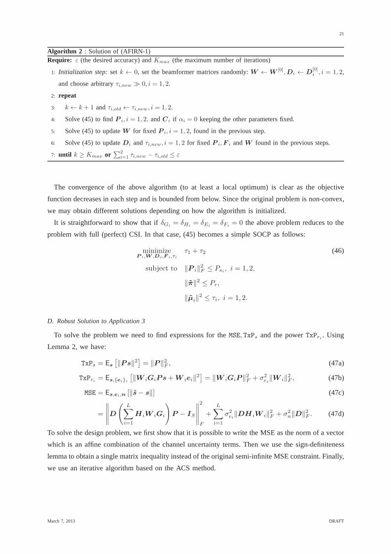
Algorithm 2 : Solution of (AFIRN-1)Require: ε (the desired accuracy) andKmax (the maximum number of iterations)

1: Initialization step: setk ← 0, set the beamformer matrices randomly:W ←W [0],Di ← D[0]i , i = 1, 2,

and choose arbitraryτi,new ≫ 0, i = 1, 2.

2: repeat

3: k ← k + 1 andτi,old ← τi,new , i = 1, 2.

4: Solve (45) to findP i, i = 1, 2, andCi if αi = 0 keeping the other parameters fixed.

5: Solve (45) to updateW for fixed P i, i = 1, 2, found in the previous step.

6: Solve (45) to updateDi andτi,new, i = 1, 2 for fixed P i,F i andW found in the previous steps.

7: until k ≥ Kmax or∑2

i=1 τi,new − τi,old ≤ ε

The convergence of the above algorithm (to at least a local optimum) is clear as the objective

function decreases in each step and is bounded from below. Since the original problem is non-convex,

we may obtain different solutions depending on how the algorithm is initialized.

It is straightforward to show that ifδGi= δHi

= δEi= δFi

= 0 the above problem reduces to the

problem with full (perfect) CSI. In that case, (45) becomes asimple SOCP as follows:

minimizeP i,W ,Di,F i,τi

τ1 + τ2 (46)

subject to ‖P i‖2F ≤ Psi , i = 1, 2,

‖π‖2 ≤ Pr,

‖µi‖2 ≤ τi, i = 1, 2.

D. Robust Solution to Application 3

To solve the problem we need to find expressions for theMSE, TxPs and the powerTxPri . Using

Lemma 2, we have:

TxPs = Es

[

‖Ps‖2]

= ‖P ‖2F , (47a)

TxPri = Es,{ei}i

[

‖W iGiPs+W iei‖2]

= ‖W iGiP ‖2F + σ2

ei‖W i‖

2F , (47b)

MSE = Es,ei,n [‖s− s‖] (47c)

=

∥

∥

∥

∥

∥

D

(

L∑

i=1

HiW iGi

)

P − IS

∥

∥

∥

∥

∥

2

F

+L∑

i=1

σ2ei‖DHiW i‖

2F + σ2

n‖D‖2F . (47d)

To solve the design problem, we first show that it is possible to write the MSE as the norm of a vector

which is an affine combination of the channel uncertainty terms. Then we use the sign-definiteness

lemma to obtain a single matrix inequality instead of the original semi-infinite MSE constraint. Finally,

we use an iterative algorithm based on the ACS method.

March 7, 2013 DRAFT

22

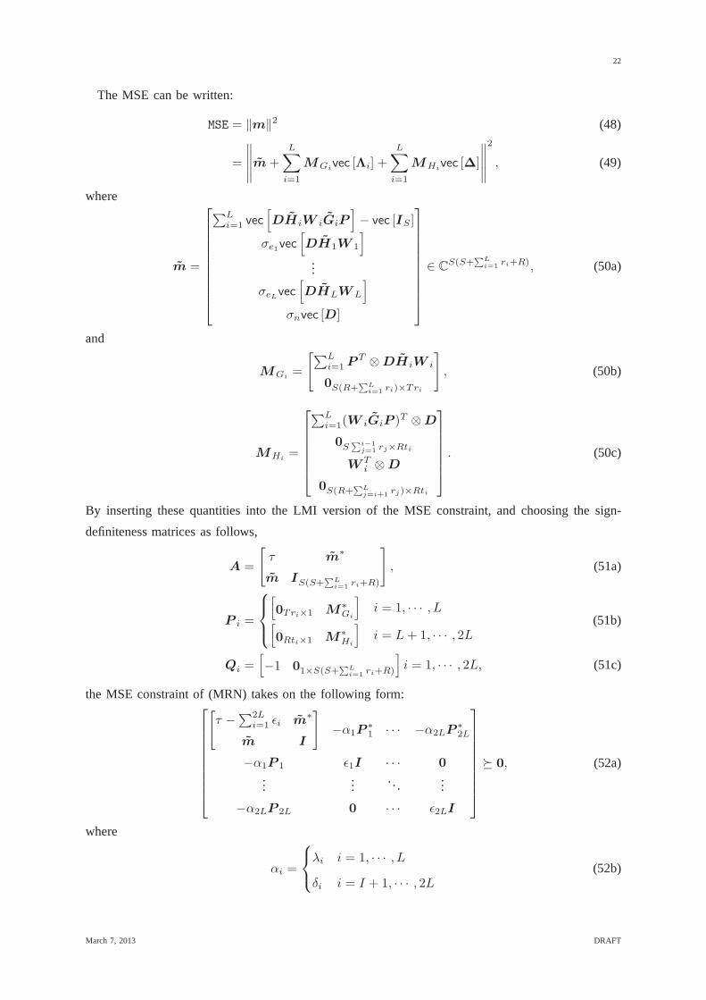
The MSE can be written:

MSE = ‖m‖2 (48)

=

∥

∥

∥

∥

∥

m+L∑

i=1

MGivec [Λi] +

L∑

i=1

MHivec [∆]

∥

∥

∥

∥

∥

2

, (49)

where

m =

∑Li=1 vec

[

DHiW iGiP]

− vec [IS]

σe1vec[

DH1W 1

]

...

σeLvec[

DHLWL

]

σnvec [D]

∈ CS(S+

∑Li=1

ri+R), (50a)

and

MGi=

[

∑Li=1P

T ⊗DHiW i

0S(R+∑

Li=1

ri)×Tri

]

, (50b)

MHi=

∑Li=1(W iGiP )T ⊗D

0S∑i−1

j=1 rj×Rti

W Ti ⊗D

0S(R+∑

Lj=i+1

rj)×Rti

. (50c)

By inserting these quantities into the LMI version of the MSEconstraint, and choosing the sign-

definiteness matrices as follows,

A =

[

τ m∗

m IS(S+∑

Li=1

ri+R)

]

, (51a)

P i =

[

0Tri×1 M∗Gi

]

i = 1, · · · , L[

0Rti×1 M∗Hi

]

i = L+ 1, · · · , 2L(51b)

Qi =[

−1 01×S(S+∑

Li=1

ri+R)

]

i = 1, · · · , 2L, (51c)

the MSE constraint of (MRN) takes on the following form:

[

τ −∑2L

i=1 ǫi m∗

m I

]

−α1P∗1 · · · −α2LP

∗2L

−α1P 1 ǫ1I · · · 0

......

. . ....

−α2LP 2L 0 · · · ǫ2LI

� 0, (52a)

where

αi =

λi i = 1, · · · , L

δi i = I + 1, · · · , 2L(52b)

March 7, 2013 DRAFT

23

Similarly for theTxPri constraint we can write

Pri − ηi p∗i 01×riti

pi I(S+ri)ti −λiΨi

0riti×1 −λiΨ∗i ηiIriti

� 0, (53a)

where

pi =

vec[

W iGiP]

σeivec [W i]

, (53b)

and

Ψi =

[

P T ⊗W i

0riti×Tri

]

. (53c)

By putting all these components together the design problembecomes

minimizeP ,D,{W i,ǫi,ηi}i,τ≥0

τ (54a)

subject to TxPs ≤ Ps, (54b)

(52a) holds,, (54c)

(53a) holds, ∀i. (54d)

Again we resort to an iterative ACS approach, summarized as follows:

Algorithm 3 : Solution of (MRN)Require: ε (the desired accuracy) andKmax (the maximum number of iterations)

1: Initialization step: setk ← 0, set the beamformer matrices randomly:W i ← W[0]i ,D ← D[0], i = 1, 2,

and choose arbitraryτnew ≫ 0.

2: repeat

3: k ← k + 1 andτold ← τnew .

4: Solve (54) to findP , keeping the other parameters fixed.

5: Solve (54) to updateW i for fixed P , found in the previous step.

6: Solve (54) to updateD andτnew for fixed P ,W i found in the previous steps.

7: until k ≥ Kmax or τnew − τold ≤ ε

E. Computational Complexity of the Proposed Algorithms

In this sub-section we give some remarks on the computational complexity of the algorithms

proposed earlier in this section. The proposed algorithms have two or three steps dealing with an

SDP. So we focus on the complexity of each SDP. Consider a real-valued SDP problem in its standard

form, i.e.,

minimizex∈Rn

cTx (55a)

subject to A0 +n∑

i=1

xiAi � 0 (55b)

March 7, 2013 DRAFT

24

whereAi are symmetric block-diagonal matrices withK blocks of dimensionak×ak . The number

of operations required to solve this SDP is upper-bounded by[47]

C

(

1 +

K∑

k=1

ak

)1/2

n

(

n2 + n

K∑

k=1

a2k +

K∑

k=1

a3k

)

, (56)

whereC is a constant that does not depend on the problem size. For example in Algorithm 1, to

compute the optimalP i in each iteration a SDP problem should be solved, for which the number

of diagonal blocksK is equal to2I. For the firstI blocks, the dimension of the block isai =

1 + TiSi; i = 1, · · · , I and for the nextI blocks the dimension of the blocks is equal toai =

1 + Si(Ri +∑I

j=1 Sj) + Ri

∑Ij=1 Tj ; i = 1, · · · , I. In this problem we should determinen =

I2 + I + 2∑I

i=1 SiTi real variables. A similar analysis can be carried out for thenext SDP in

Algorithm 1, and also for the other algorithms.

In order to obtain some insight from (56), let us assume that the network has a large number of

users (I ≫ 1), and that the number of transmit and receive antennas is larger than the number of

independent streams of each link (Ti, Ri ≥ Si). Also assume that we have a fully symmetric network,

i.e., all the nodes have an equal number of antennas and streams (Si = S, Ti = T,Ri = R,∀i). In

this case, the required number of operations to get the precoder matrix is roughly

K × I5 × S × T 4.5 ×R3.5, (57)

where K is a constant. Hence in this example, doubling the number of data streams and trans-

mit/receive antennas, increases the complexity by a factorin the order of29 ∼ 500.

V. SIMULATION RESULTS

To illustrate the performance of the algorithm proposed in Section IV, we present here detailed

numerical results for the interfering relay scenario in Section II-C. The simulation setup is as follows.

The system is used to transferS1 = S2 = 2 streams of independent data symbols between the source

and the destination. The numbers of transmit and receive antennas at the source, relay and destination

nodes are equal toTi = Ri = t = r = 4, i = 1, 2. Both the source and relay power budgets are set

to Pr = Ps1 = Ps2 = 1. The convergence parameters of the algorithm are set toKmax = 1000, and

ε = 10−4. We will present results for the case whenα = 1, i.e., for a Gaussian IRC. The initial value

of the relay precoder and the destination equalizer matrices are chosen at random. Due to the long

computation time, we obtained the results by fixing the channel realization (at random) and averaging

over 10000 perturbations. As for the distribution of the perturbations, we tried both Gaussian random

matrices with a standard deviation proportional to the uncertainty size, and matrices on the sphere of

uncertainty around the nominal value of the channel. These two choices yielded very similar results.

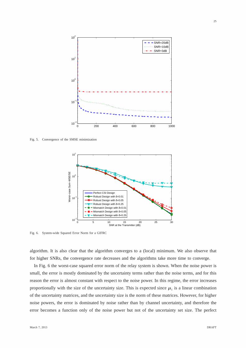
To demonstrate the convergence of the proposed algorithm, the empirical SMSE of the system

as a function of the number of iterations is shown in Fig. 5. This figure shows the convergence of

the algorithm forδGi= δHi

= δEi= δFi

= 0.01 and different SNRs of 3 dB, 10 dB, and 20 dB

(σ2ei = σ2

u = −3 dB,−10 dB,−20 dB). It is clear that at each iteration, the SMSE of the system

decreases. After a few iterations the rate of change of the SMSE is small enough to terminate the

March 7, 2013 DRAFT

25

0 200 400 600 800 100010

−2

10−1

100

101

102

SNR=20dBSNR=10dBSNR=3dB

Fig. 5. Convergence of the SMSE minimization

0 5 10 15 20 25 3010

−2

10−1

100

101

SNR at the Transmitter (dB)

Wor

st−

case

Sum

−M

SE

/SE

Perfect CSI Design

Robust Design with δ=0.01

Robust Design with δ=0.05

Robust Design with δ=0.25

Mismatch Design with δ=0.01

Mismatch Design with δ=0.05

Mismatch Design with δ=0.25

Fig. 6. System-wide Squared Error Norm for a GIFRC

algorithm. It is also clear that the algorithm converges to a(local) minimum. We also observe that

for higher SNRs, the convergence rate decreases and the algorithms take more time to converge.

In Fig. 6 the worst-case squared error norm of the relay system is shown. When the noise power is

small, the error is mostly dominated by the uncertainty terms rather than the noise terms, and for this

reason the error is almost constant with respect to the noisepower. In this regime, the error increases

proportionally with the size of the uncertainty size. This is expected sinceµi is a linear combination

of the uncertainty matrices, and the uncertainty size is thenorm of these matrices. However, for higher

noise powers, the error is dominated by noise rather than by channel uncertainty, and therefore the

error becomes a function only of the noise power but not of theuncertainty set size. The perfect

March 7, 2013 DRAFT

26

0 5 10 15 20 25 3010

−3

10−2

10−1

100

101

SNR at the Transmitter (dB)

Wor

st−

case

Sum

−M

SE

/SE

Perfect CSI Design

Robust Design with δ=0.01

Robust Design with δ=0.05

Robust Design with δ=0.25

Mismatch Design with δ=0.01

Mismatch Design with δ=0.05

Mismatch Design with δ=0.25

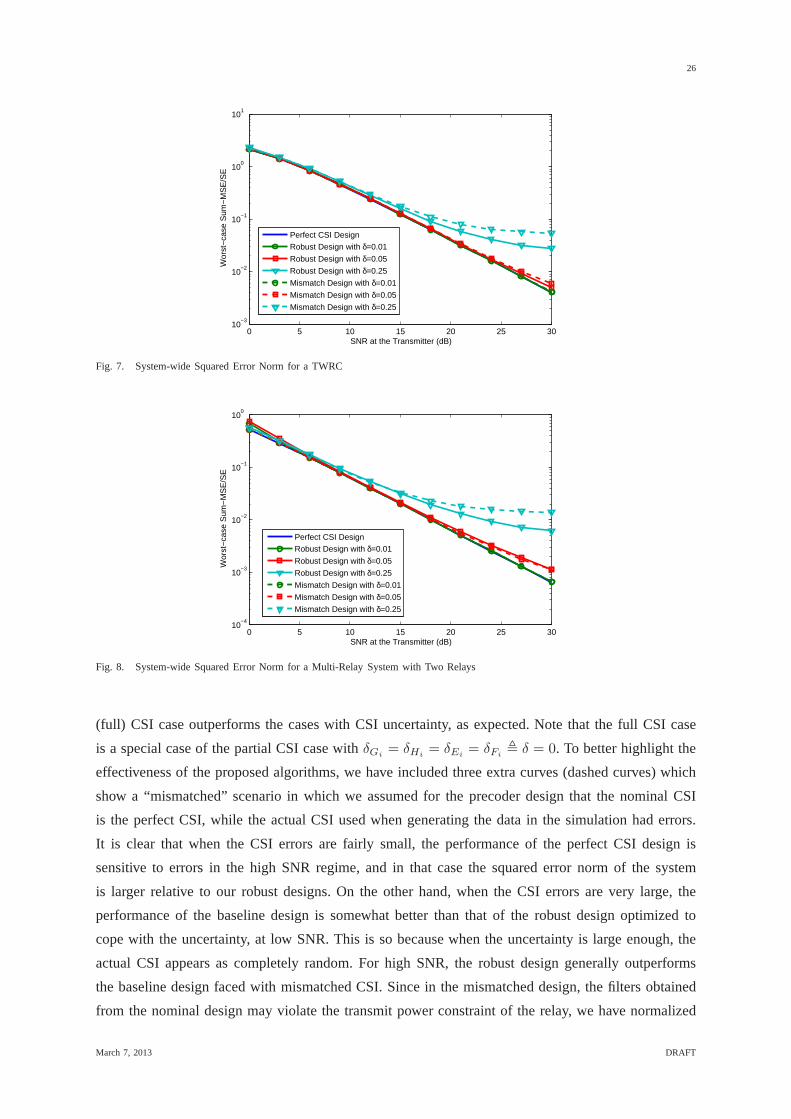
Fig. 7. System-wide Squared Error Norm for a TWRC

0 5 10 15 20 25 3010

−4

10−3

10−2

10−1

100

SNR at the Transmitter (dB)

Wor

st−

case

Sum

−M

SE

/SE

Perfect CSI Design

Robust Design with δ=0.01

Robust Design with δ=0.05

Robust Design with δ=0.25

Mismatch Design with δ=0.01

Mismatch Design with δ=0.05

Mismatch Design with δ=0.25

Fig. 8. System-wide Squared Error Norm for a Multi-Relay System with Two Relays

(full) CSI case outperforms the cases with CSI uncertainty,as expected. Note that the full CSI case

is a special case of the partial CSI case withδGi= δHi

= δEi= δFi

, δ = 0. To better highlight the

effectiveness of the proposed algorithms, we have includedthree extra curves (dashed curves) which

show a “mismatched” scenario in which we assumed for the precoder design that the nominal CSI

is the perfect CSI, while the actual CSI used when generatingthe data in the simulation had errors.

It is clear that when the CSI errors are fairly small, the performance of the perfect CSI design is

sensitive to errors in the high SNR regime, and in that case the squared error norm of the system

is larger relative to our robust designs. On the other hand, when the CSI errors are very large, the

performance of the baseline design is somewhat better than that of the robust design optimized to

cope with the uncertainty, at low SNR. This is so because whenthe uncertainty is large enough, the

actual CSI appears as completely random. For high SNR, the robust design generally outperforms

the baseline design faced with mismatched CSI. Since in the mismatched design, the filters obtained

from the nominal design may violate the transmit power constraint of the relay, we have normalized

March 7, 2013 DRAFT

27

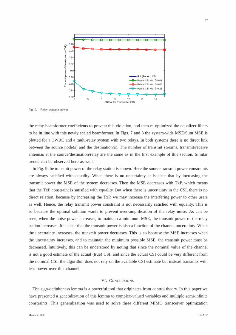
18151296300.82

0.84

0.86

0.88

0.9

0.92

0.94

0.96

0.98

1

SNR at the Transmitter (dB)

Tra

nsm

it po

wer

of t

he r

elay

nod

e (T

xPr)

Full (Perfect) CSI

Partial CSI with δ=0.01

Partial CSI with δ=0.05

Partial CSI with δ=0.25

Fig. 9. Relay transmit power

the relay beamformer coefficients to prevent this violation, and then re-optimized the equalizer filters

to be in line with this newly scaled beamformer. In Figs. 7 and8 the system-wide MSE/Sum MSE is

plotted for a TWRC and a multi-relay system with two relays. In both systems there is no direct link

between the source node(s) and the destination(s). The number of transmit streams, transmit/receive

antennas at the source/destination/relay are the same as inthe first example of this section. Similar

trends can be observed here as well.

In Fig. 9 the transmit power of the relay station is shown. Here the source transmit power constraints

are always satisfied with equality. When there is no uncertainty, it is clear that by increasing the

transmit power the MSE of the system decreases. Then the MSE decreases with TxP, which means

that the TxP constraint is satisfied with equality. But when there is uncertainty in the CSI, there is no

direct relation, because by increasing the TxP, we may increase the interfering power to other users

as well. Hence, the relay transmit power constraint is not necessarily satisfied with equality. This is

so because the optimal solution wants to prevent over-amplification of the relay noise. As can be

seen, when the noise power increases, to maintain a minimum MSE, the transmit power of the relay

station increases. It is clear that the transmit power is also a function of the channel uncertainty. When

the uncertainty increases, the transmit power decreases. This is so because the MSE increases when

the uncertainty increases, and to maintain the minimum possible MSE, the transmit power must be

decreased. Intuitively, this can be understood by noting that since the nominal value of the channel

is not a good estimate of the actual (true) CSI, and since the actual CSI could be very different from

the nominal CSI, the algorithm does not rely on the availableCSI estimate but instead transmits with

less power over this channel.

VI. CONCLUSIONS

The sign-definiteness lemma is a powerful tool that originates from control theory. In this paper we

have presented a generalization of this lemma to complex-valued variables and multiple semi-infinite

constraints. This generalization was used to solve three different MIMO transceiver optimization

March 7, 2013 DRAFT

28

problems, namely that of interfering adhoc networks, general relay networks, and relay networks

with multiple relays. We considered a (sum) MSE problem formulation in all three applications,

and we have seen that the corresponding optimization problems are non-convex and semi-infinite.

We used the sign-definiteness lemma to relax the semi-infiniteness of problems and we resorted to

iterative algorithms based on ACS to devise a practical algorithm for solving the design problems.

Simulation results show that when increasing the noise power and when increasing the size of the

CSI uncertainty set, then the (sum) MSE increases. In the high SNR regime (where the noise power

is low) the SMSE and the optimal transmit power are mainly affected by the CSI uncertainty set

size. By contrast, at low SNR, the uncertainty size does not play an important role for the behavior

of these quantities.

REFERENCES

[1] S. Skogestad, and I. Postlethwaite,Multivariable Feedback Control - Analysis and Design, John Wiley & Sons, 1996.

[2] K. Zhou, Essentials of robust control, Prentice Hall, 1997.

[3] M. Bengtsson and B. Ottersten, “Optimal downlink beamforming using semidefinite optimization,”Proceedings of 37th Annual

Allerton Conference on Communication, Control, and Computing, pp. 987-996, Sep. 1999.

[4] S. A. Vorobyov, A. B. Gershman and Z. -Q. Luo, “Robust adaptive beamforming using worst-case performance optimization: A

solution to the signal mismatch problem,”IEEE Transactions On Signal Processing, vol. 51, no. 2, pp. 313-324, 2003.

[5] S. A. Vorobyov, A. B. Gershman, Z. -Q. Luo and N. Ma, “Adaptive beamforming with joint robustness against mismatched signal

steering vector and interference nonstationarity,”IEEE Signal Processing Letters, vol. 11, no. 2, pp. 108-111, 2004.

[6] S. A. Vorobyov, H. Chen and A. B. Gershman, “On the relationship between robust minimum variance beamformers with probabilistic

and worst-case distortionless response constraints,”IEEE Transactions On Signal Processing, vol. 56, no. 11, pp. 5719-5724, 2008.

[7] V. Sharma, I. Wajid, A. B. Gershman, H. Chen and S. Lambotharan, “Robust downlink beamforming using positive semidefinite

covariance constraints,”Proceedings of 2008 International ITG Workshop on Smart Antenna (WSA 2008), pp. 36-41, Feb. 2008.

[8] J. Li, P. Stoica, and Z. Wang “On robust Capon beamformingand diagonal loading,”IEEE Trans. Signal Processing, vol. 51 , no. 7,

pp. 1702-1715, Jul. 2003.

[9] A.B. Gershman, Z.-Q. Luo, and S. ShahbazPanahi, “Robustadaptive beamforming using worst-case performance optimization,”

chapter in the bookRobust Adaptive Beamforming, P. Stoica and J. Li (Editors), John Wiley & Sons, August 2005.

[10] S. ShahbazPanahi, A.B. Gershman, Z.-Q. Luo, and K.M. Wong, “Robust adaptive beamforming for general-rank signal models,”IEEE

Transactions on Signal Processing, vol. 51, pp. 2257-2269, Sept. 2003.

[11] A. Abdel-Samad, T.N. Davidson, and A.B. Gershman, “Robust transmit eigen beamforming based on imperfect channel state

information,” IEEE Trans. Signal Processing, vol. 54, no. 5, pp. 1596-1609, May 2006

[12] A. Mutapcic, S. -J. Kim and S. Boyd, “A tractable method for robust downlink beamforming in wireless communications,” Proceedings

of 2007 Asilomar Conference on Signals, Systems, and Computers (ACSSC 2007), pp. 1224-1228, Nov. 2007.

[13] S. -J. Kim, A. Magnani, A. Mutapcic, S. P. Boyd and Z. -Q. Luo, “Robust beamforming via worst-case SINR maximization”IEEE

Transactions On Signal Processing, vol. 56, no. 4, pp. 1539-1574, 2008.

[14] I.R. Petersen, “A stabilization algorithm for a class of uncertain linear systems,”Systems & Control Letters, no. 8, pp. 351-357, 1987.

[15] M.B. Shenouda, and T.N. Davidson, “Robust linear precoding for uncertain MISO broadcast channels,”in Proc. ICASSP 2006,

Toulouse, France, May 2006.

[16] M. Payaro, A. Pascual-Iserte, and M.A. Lagunas, “Robust power allocation designs for multiuser and multiantenna downlink

communication systems through convex optimization,”IEEE J. Sel. Areas Commun., vol. 25, no. 7, pp. 1390–1401, Sep. 2007.

[17] N. Vucic and H. Boche, “Robust QoS-constrained optimization of downlink multiuser MISO systems,”IEEE Trans. Signal Process.,

vol. 57, no. 2, pp. 714–725, Feb. 2009.

[18] M.B. Shenouda, and T.N. Davidson, “Convex conic formulations of robust downlink precoder design with quality of service

constraints,”IEEE J. Sel. Topics Signal Process., vol. 1, no. 4, pp. 714–724, Dec. 2007.

[19] E.A. Gharavol, Y.-C. Liang, and K. Mouthaan, “Robust downlink beamforming in multiuser MISO cognitive radio networks with

imperfect channel state information,”IEEE Trans. Vehicular Tech., vol. 59, No. 6, July 2010.

March 7, 2013 DRAFT

29

[20] Y. Guo, and B.C. Levy, “Robust MSE equalizer design for MIMO communication systems in the presence of model uncertainties,

IEEE Trans. Signal Process., vol. 54, no. 5, pp. 1840–1852, May 2006.

[21] N. Vucic, H. Boche, and S. Shi, “Robust transceiver optimization in downlink multiuser MIMO systems,”IEEE Tran. Signal Process.,

vol. 57, no. 9, pp. 3576-3587, Sep. 2009.

[22] P. Ubaidulla, and A. Chockalingam, “Robust transceiver design for multiuser MIMO downlink,”Proc. IEEE Global Telecommunica-

tions Conference, pp.1-5, Nov. 2008.

[23] J. Liu, and Z. Qiu, “Robust sum-MSE transceiver optimisation for multi-user non-regenerative MIMO relay downlinksystems,”

Electronics Letters, vol. 47, no. 6, pp. 411-412, Mar. 2011.

[24] T.E. Bogale, B.K. Chalise, and L. Vandendorpe, “Robusttransceiver optimization for downlink multiuser MIMO systems,” IEEE

Trans. Signal Processing, vol. 59, no. 1, pp. 446-453, Jan. 2011.

[25] E.A.Gharavol, Y.-C- Liang, and K. Mouthaan, “Robust linear transceiver design in MIMO adhoc cognitive radio networks with

imperfect state information,”IEEE Trans. Wireless Comm., vol. 10, No. 5, May 2011.

[26] Y.C. Eldar, A. Ben-Tal, and A. Nemirovski, “Robust mean-squared error estimation in the presence of model uncertainties,” IEEE

Tran. Signal Processing, vol. 53, no. 1, Jan. 2005.

[27] F. Gao, R. Zhang, and Y.-C. Liang, “Optimal channel estimation and training design for two-way relay networks,”IEEE Trans.

Communications, vol. 57, no. 10, pp. 3024-3033, Oct. 2009.

[28] —–, “Channel estimation for OFDM modulated two-way relay networks,” IEEE Trans. Signal Processing, vol. 57, no. 11, pp.

4443-4455, Nov. 2009.

[29] B. Jiang, F. Gao, X. Gao, and A. Nallanathan, “Channel estimation and training design for two-way relay networks with power

allocation,” IEEE Trans. Wireless Communications, vol. 9, no. 6, pp. 2022-2032, Jun. 2010.

[30] T. Cui, F. Gao, T. Ho, and A. Nallanathan, “Distributed space-time coding for two-way wireless relay networks,”IEEE Trans. Signal

Processing, vol. 57, no. 2, pp. 658-671, Feb. 2009.

[31] V. Havary-Nassab, S. Shahbazpanahi, and A. Grami, “Optimal distributed beamforming for two-way relay networks,”IEEE Trans.

Signal Processing, vol.58, no.3, pp.1238-1250, Mar. 2010.

[32] J. Joung, and A.H. Sayed, “Multiuser two-way amplify-and-forward relay processing and power control methods for beamforming

systems,”IEEE Trans. on Signal Processing, vol.58, no.3, pp.1833-1846, Mar. 2010.

[33] I. Krikidis, and J.S Thompson, “MIMO two-way relay channel with superposition coding and imperfect channel estimation,” Proc.

IEEE GLOBECOM Workshops pp. 84-88, Dec. 2010.

[34] A.Y. Panah, and R.W. Heath, “MIMO two-way amplify-and-forward relaying with imperfect receiver CSI,”IEEE. Trans. Vehicular

Technology, vol. 59, no. 9, pp. 4377-4387, Nov. 2010.

[35] —–, “Sum-rate of MIMO two-way relaying with imperfect CSI,” Proc. IEEE Conf. Acoustics Speech and Signal Processing (ICASSP),

pp. 3418-3421, Mar. 2010.

[36] Y. Tian, and A. Yener, “The Gaussian interference relaychannel: improved achievable rates and sum rate upper bounds using a potent

relay,” IEEE Trans. Information Theory, vol. 57, no. 5, pp. 2865-2879, May 2011.

[37] S. Sridharan, S. Vishwanath, S.A. Jafar, and S. Shamai,“On the capacity of cognitive relay assisted Gaussian interference channel,”

Proc. IEEE Information Theory Symp., pp. 549-553, Jul. 2008.

[38] I. Maric, R. Dabora, and A.J. Goldsmith, “An outer boundfor the Gaussian interference channel with a relay,”Proc. IEEE Information

Theory Workshop, pp. 569-573, Oct. 2009.

[39] O. Simeone, O. Sahin, and E. Erkip, “Interference channel aided by an infrastructure relay,”Proc. Information Theory Symp., pp.

2023-2027, Jun. 2009.

[40] Y. Shi, J.H. Wang, W.L. Huang, and K. Ben Letaief, “Powerallocation in Gaussian interference relay channels via game theory,”

Proc. IEEE Global Telecommunications Conf., pp. 1-5, Nov. 2008.

[41] Y. Shi, J. Wang, K. Letaief, and R. Mallik, “A game-theoretic approach for distributed power control in interference relay channels,”

IEEE Trans. Wireless Communications, vol. 8, no. 6, pp. 3151-3161, Jun. 2009.

[42] P. Razaghi, and W. Yu “Universal relaying for the interference channel,”Proc. Information Theory and Applications Workshop, pp.

1-6, Jan. 2010.

[43] E.G. Larsson, E.A. Jorswieck, J. Lindblom, and R. Mochaourab, “Game theory and the flat-fading Gaussian interference channel:

analyzing resource conflicts in wireless networks,”IEEE Signal Processing Magazine, vol. 26, no. 5, pp. 18-27, Sept. 2009.

[44] F. Roemer, and M. Haardt, “Algebraic norm-maximizing (ANOMAX) transmit strategy for two-way relaying with MIMO amplify

and forward relays,”IEEE Signal Processing Letters, vol. 16, pp. 909-912, Oct. 2009.

March 7, 2013 DRAFT

30

[45] J. Li, F. Roemer, and M. Haardt, “Efficient Relay Sharing(EReSh) between multiple operators in amplify-and-forward relaying

systems,”Proc. IEEE 4th Int. Workshop on Computational Advances in Multi-Sensor Adaptive Processing (CAMSAP 2011), pp.

249-252, Dec. 2011.

[46] K. B. Petersen and M. S. Pedersen,The Matrix Cookbook, Technical University of Denmark, Oct. 2008.

[47] A. Ben-Tal, and A. Nemirovski,Lectures on Modern Convex Optimization: Analysis, Algorithms, and Engineering Applications, ser.

MPS-SIAM Series on Optimization, 2001.

[48] W.J. Mao, and J. Chu, “Quadratic stability and stabilization of dynamic interval systems,”IEEE Trans. Automatic Control, vol. 48,

no. 6, Jun. 2003.

[49] M.V. Khlebnikov, and P.S. Shcherbakov, “Petersen’s lemma on matrix uncertainty and its generalizations,”Automation and Remote

Control, vol. 69, no. 11, pp. 1932–1945, 2008.

[50] S. Boyd, L. El Ghaoui, E. Ferron, and V. Balakrishnan,Linear Matrix Inequalities in System and Control Theory, Philadelphia, PA:

SIAM, 1994.

[51] Z.-Q. Luo, W.-K. Ma, A.M.-C. So, Y. Ye, and S. Zhang “Semidefinite relaxation of quadratic optimization problems,”IEEE Signal

Processing Mag., vol. 27, no. 3, pp. 20-34, May 2010.

[52] J. Gorski, F. Pfeuffer, and K. Klamroth, “Biconvex setsand optimization with biconvex functions - a survey and extensions,”

Mathematical Methods of Operations Research, vol. 66, no. 3., pp. 373-408, Dec. 2007.

[53] M. Joham, P.M. Castro, L. Castedo, and W. Utschick, “Robust precoding with Bayesian error modeling for limited feedback MU-MISO

systems,”IEEE Trans. Signal Processing, vol. 48, no. 9, pp. 4954-4960, Sept. 2010.

[54] N. Farvardin, “A study of vector quantization for noisychannels,”IEEE Trans. Information Theory vol. 36 , no. 4, pp. 799-809, 1990.

[55] M. Gastpar, B. Rimoldi, and M. Vetterli, “To code, or notto code: lossy source channel communication revisited,”IEEE Trans.

Information Theory, vol. 49, no. 5, pp. 1147-1158, May 2003.

[56] D. Persson, J. Kron, M. Skoglund, and E.G. Larsson, “Joint source-channel coding for the MIMO broadcast channel,”IEEE Trans.

Signal Processing, vol. 60, no. 4, pp. 2085-2090, Apr. 2012.

[57] A. Lozano, and N. Jindal, “Transmit diversity vs. spatial multiplexing in modern MIMO systems,”IEEE Trans. Wireless

Communications, vol. 9, no. 1, pp. 186-197, Jan. 2010.

[58] K.G. Murty, and S.N. Kabadi, “Some NP-Complete problems in quadratic and nonlinear programming,”Mathematical Programming,

no. 39, pp. 117-129, 1987.

[59] I.G. Akrotiriankis, and C.A. Floudas, “A new class of improved convex under-estimators for twice continuously differentiable

constrained NLPs,”Journal of Global Optimization, no. 20, pp. 367-390, 2004.

[60] D. Bertsimas, and M. Sim, “Tractable approximations torobust conic optimization problems,”Mathematical Programming, vol. 1,

no. 107, pp. 5-36, 2006.

[61] E.A. Gharavol, and E.G. Larsson, “Robust joint optimization of MIMO two-way relay channels with imperfect CSI,”Proc. Allerton

Conf. on Communication, Control, and Computing, pp. 1657 - 1664, Sept. 2011.

[62] E.A. Gharavol, and E.G. Larsson, “Robust joint optimization of non-regenerative MIMO relay channels with imperfect CSI”, Proc.

of the 45th Annual Asilomar Conf. Signals, Systems, and Computers, 2011.

[63] E.A. Gharavol, and E.G. Larsson, “Robust joint optimization of MIMO interfering relay channels with imperfect CSI,” Proc. 4th

IEEE International Workshop on Computational Advances in Multi-Sensor Adaptive Processing, pp. 209-212, Dec. 2011.

March 7, 2013 DRAFT