Embed Size (px)
Citation preview

The Sloan Digital Sky Survey
Robert Lupton
Xiaohui Fan
Jim Gunn
Zeljko Ivezic
Jill Knapp
Michael Strauss
· · ·
University of Chicago,Fermilab,
Institute for Advanced Study,Japanese Participation Group,
Johns Hopkins University,Los Alamos National Laboratory,
Max-Planck Institute (MPIA),Max-Planck Institute (MPA),New Mexico State University
University of PittsburgPrinceton University,
United States Naval Observatory,University of Washington
Irvine, June 2002
1

Objectives
• Map the large scale structure of the Universe
• Survey the Northern Galactic Cap (104 square degrees) in
five bands (u’ g’ r’ i’ z’) to PSF magnitude limits of 22.3,
23.3, 23.1, 22.3, and 20.8
• Obtain astrometry good to ∼ 30mas/coordinate
• Spectroscopic survey at a resolution R ≈ 2000 of
– 106 galaxies:
– 105 QSOs
– few ×104 stars
2

Objectives
• Make images and associated catalogs of 1/4 of the entire sky,namely that part away from the Milky Way, and visible fromthe northern hemisphere. We expect to detect and measurewell over 108 galaxies, and a similar number of stars.
• Try to use all photons that pass through the atmosphere, butnot through silicon; basically 310nm—1050nm. At peak, wedetect about 50% of photons that fall on the primary mirror.
• Obtain images of stars a few million times fainter than thosejust visible to the naked eye on a dark night.
• Obtain spectra for 106 galaxies, 105 quasars, and a few ×104
stars. These spectra tell us the radial velocities (and hencedistances to the galaxies and quasars), but they also tell usa lot about the objects’ physical conditions.
3

Instrumentation
• A telescope (with a 2.5m diameter primary mirror) at ApachePoint, New Mexico
• A camera containing
– 30 2048× 2048 photometric CCDs;∗
u’ g’ r’ i’ z’ filters
– 24 2048× 400 astrometric and focus CCDs
– Lots of Electronics, Quartz, Liquid Nitrogen, and Vacuum
• Two 320-fibre-fed double spectrographs, each with two 2048×2048 CCDs
• Lots of software
∗Charge Coupled Devices
4

Software
The software was a difficult technical challenge on this project;probably harder than building the telescope and camera.∗
• Moderately large data volumes:
– 20Gb/hr when imaging
– 10-15 Tb over the course of the survey
• Data is taken under varying conditions, but the great strengthof a dedicated survey such as SDSS is producing a uniformdataset.
• We are sensitive to the (non-Gaussian) tails of distributions;for example 4 objects with particular properties out of 15million.
∗I don’t count building a functioning collaboration between scientists and institutions as atechnical challenge
5

The spiral galaxy NGC428
The image maps the i-r-g filters to RGB, so what appears as a
tasteful bluish-cyan is really dominated by the strong emission
lines of [OIII] (5007A) and Hα (6563A).
6

A cluster of galaxies
7
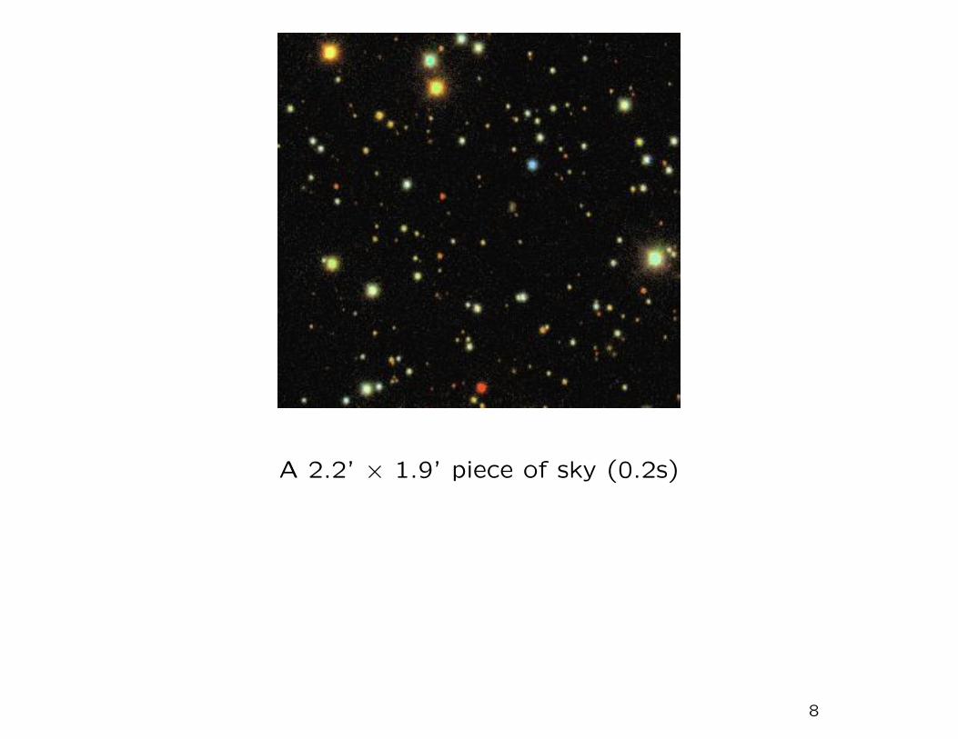
A 2.2’ × 1.9’ piece of sky (0.2s)
8

These are all very nice, but:
Why Bother?
9
Why Bother?
• Doesn’t the Hubble Space Telescope do all this?
10

Why Bother?
• Doesn’t the Hubble Space Telescope do all this?
• No; it produces exquisite images of tiny pieces of the sky.
We produce OK images of large chunks of the sky.
11
Why Bother?
• Doesn’t the Hubble Space Telescope do all this?
• No; it produces exquisite images of tiny pieces of the sky.
We produce OK images of large chunks of the sky.
• What about those enormous telescopes in Hawai‘i and Chile?
12

Why Bother?
• Doesn’t the Hubble Space Telescope do all this?
• No; it produces exquisite images of tiny pieces of the sky.
We produce OK images of large chunks of the sky.
• What about those enormous telescopes in Hawai‘i and Chile?
• They’re great for catching photons, and some of they are
producing images almost as good as HST (maybe better
in the IR); but they’re still looking in great detail at small
patches of the sky.
13

Why Bother?
• Doesn’t the Hubble Space Telescope do all this?
• No; it produces exquisite images of tiny pieces of the sky.
We produce OK images of large chunks of the sky.
• What about those enormous telescopes in Hawai‘i and Chile?
• They’re great for catching photons, and some of they are
producing images almost as good as HST (maybe better
in the IR); but they’re still looking in great detail at small
patches of the sky.
• But the patches are so far away that they represent a large
volume, right?
14

Why Bother?
• Doesn’t the Hubble Space Telescope do all this?
• No; it produces exquisite images of tiny pieces of the sky.We produce OK images of large chunks of the sky.
• What about those enormous telescopes in Hawai‘i and Chile?
• They’re great for catching photons, and some of they areproducing images almost as good as HST (maybe betterin the IR); but they’re still looking in great detail at smallpatches of the sky.
• But the patches are so far away that they represent a largevolume, right?
• Right; but it’s a volume of the Universe that’s only a fewGigayears old. SDSS can tell you what the local Universe isdoing now and we need to know both.
15

OK, so SDSS is unique, but how does it Advance Astronomy?
or
Are Pretty Pictures Science?
16

Stars (and galaxies) lie in quite well-defined parts of colourn
space. In many cases, the colours tell us much of what we want
to know. For example, blue stars are hot; red stars are cool.
All the stellar objects detected in about 2.5 degrees2 of sky;
yellow–red colour v. red–infrared colour
17

Colours are not always good enough...
A-type star White Dwarf
Both of these stars have a similar temperature, but the radii (and
therefore luminosities L ∼ R2T4) are very different.
18

But not all blue point-like objects are stars...
A Quasar at a redshift z of about 3 (i.e. λ = (1 + z)λ0 ≈ 4λ0)
The prominent emission line at ≈ 5000A is Lyα, the fundamental
n = 2→ 1 transition of hydrogen. The spectrum to the blue (i.e.
left) of Lyα shows absorption by neutral hydrogen between us and
the quasar.
19

The yellow represents neutral and the white ionized hydrogen;quasars are magenta and you are sitting at the right-hand-sideof the page. Quasars that are further away (higher z; further tothe left) pass through more hydrogen and therefore more of thelight that they emit to the blueward of Lyα is absorbed.
20

And not all quasars are blue (or bright)
gri (green–red–near infrared) riz (red–near infrared–less nearinfrared)
A quasar at z ≈ 6.28; all the visible and near infrared light is
absorbed by intervening neutral hydrogen.
Hint: Look between the star and the galaxy, and down a little
21

Becker et al.
2001, AJ, 122, 2850
� ��� �
�������� ��������� ��������� � �� � ����! �"$#�% &('�)+*-,.��/�0������ 1��2 ���3� �4657� �08:9 ���;�<�=?>�@2AB�DC �08 E 1��� ���3� �4F"G�����H �I 8 �� � �� � ����J���$�0�K �L8 �� � NM$OP � �RQ� ��TSVU �
22

Not all weird-coloured objects are at cosmological distances;
some are asteroids in our solar system.
The images map the i-r-g filters to RGB. The data is taken in
the order riuzg, i.e. GR··B
23
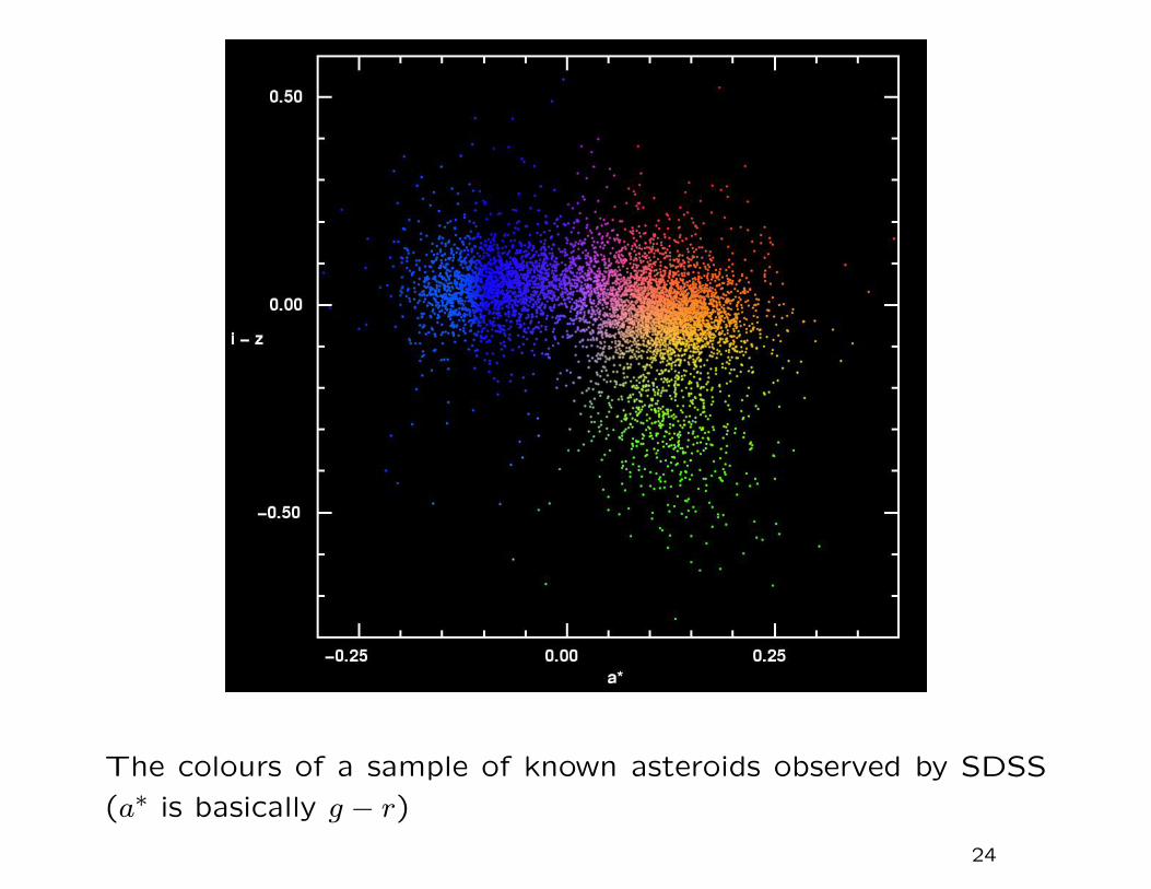
The colours of a sample of known asteroids observed by SDSS
(a∗ is basically g − r)24
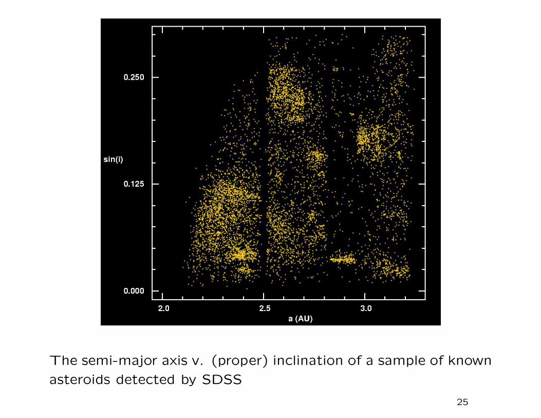
The semi-major axis v. (proper) inclination of a sample of known
asteroids detected by SDSS
25

The semi-major axis v. (proper) inclination of a sample of known
asteroids detected by SDSS
26

The End
or (more accurately)
Time for me to make way for Eva Grebel and Daniel Eisenstein
27

Field 2570 4 194; 10’ × 13’; 7s of SDSS imaging
28
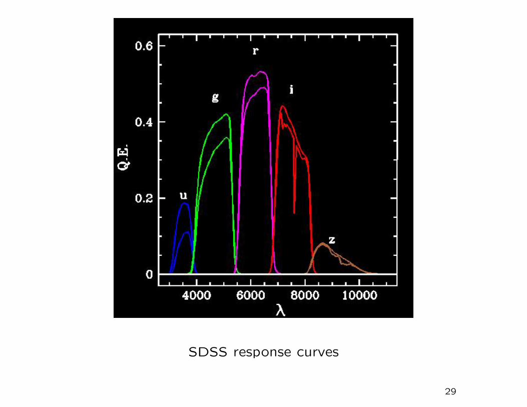
SDSS response curves
29

In each panel, the bottom-left image is the gri colour-composite
of an ‘object’ from the SDSS imaging data. The other two
panels show the decomposition of this composite into objects
that are measured and catalogued by the SDSS software.
An asteroid passing a star A fast asteroid passing a star
The images map the i-r-g filters to RGB. The data is taken in
the order riuzg, i.e. GR··B30

All the stars detected in about 2.5 square degrees of sky;
yellow–red colour v. brightness
31

10� -2 10� -1 10� 0 10� 1 10� 2 10� 3
100
101
102
103
104
105
106
107
108
109
1010
1011
1012
Farinella et al. 92 (1)Farinella et al. 92 (2)Farinella et al. 92 (3)Farinella et al. 92 (4) Galileo teamDavis et al. 94Durda et al 98. ModelSAM99 ModelSDSS 2001
<----
- LARGE SIZEBUMP
<----
SMALL SIZEBUMP
D (km)
CU
MU
LAT
IVE
NU
MB
ER
> D
COMPARISON OF ASTEROID SIZE DISTR� IBUTION: OBSERVATIONS AND MODELS
The asteroid size distribution (Davis 2002, in Asteroids III).
SDSS results:1) Extended the observed range to ∼300m2) Detected the second break at ∼5 km
32

1 101 10
The impact rate for D>1 km: once in a million years
33