arX

iv:a

stro

-ph/

0006

396v

1 2

7 Ju

n 20

00

The Sloan Digital Sky Survey: Technical Summary

Donald G. York1, J. Adelman2, John E. Anderson, Jr.2, Scott F. Anderson3, James Annis2,

Neta A. Bahcall4, J. A. Bakken2, Robert Barkhouser5, Steven Bastian2, Eileen Berman2,

William N. Boroski2, Steve Bracker2, Charlie Briegel2, John W. Briggs6, J. Brinkmann7,

Robert Brunner8, Scott Burles1, Larry Carey3, Michael A. Carr4, Francisco J. Castander1,9,

Bing Chen5, Patrick L. Colestock2, A. J. Connolly10, J. H. Crocker5, Istvan Csabai5,11,

Paul C. Czarapata2, John Eric Davis7, Mamoru Doi12, Tom Dombeck1, Daniel

Eisenstein13,1,14, Nancy Ellman15, Brian R. Elms4,16, Michael L. Evans3, Xiaohui Fan4,

Glenn R. Federwitz2, Larry Fiscelli1, Scott Friedman5, Joshua A. Frieman2,1, Masataka

Fukugita17,13, Bruce Gillespie7, James E. Gunn4, Vijay K. Gurbani2, Ernst de Haas4, Merle

Haldeman2, Frederick H. Harris18, J. Hayes7, Timothy M. Heckman5, G. S. Hennessy19,

Robert B. Hindsley20, Scott Holm2, Donald J. Holmgren2, Chi-hao Huang2, Charles Hull21,

Don Husby2, Shin-Ichi Ichikawa16, Takashi Ichikawa22, Zeljko Ivezic4, Stephen Kent2, Rita

S.J. Kim4, E. Kinney7, Mark Klaene7, A. N. Kleinman7, S. Kleinman7, G. R. Knapp4, John

Korienek2, Richard G. Kron1,2, Peter Z. Kunszt5, D.Q. Lamb1, B. Lee2, R. French Leger3,

Siriluk Limmongkol3, Carl Lindenmeyer2, Daniel C. Long7, Craig Loomis7, Jon Loveday1,

Rich Lucinio7, Robert H. Lupton4, Bryan MacKinnon2,23, Edward J. Mannery3, P. M.

Mantsch2, Bruce Margon3, Peregrine McGehee24, Timothy A. McKay25, Avery Meiksin26,

Aronne Merelli27, David G. Monet18, Jeffrey A. Munn18, Vijay K. Narayanan4, Thomas

Nash2, Eric Neilsen5, Rich Neswold2, Heidi Jo Newberg2,28, R. C. Nichol27, Tom

Nicinski2,29, Mario Nonino30, Norio Okada16, Sadanori Okamura12, Jeremiah P. Ostriker4,

Russell Owen3, A. George Pauls4, John Peoples2, R. L. Peterson2, Donald Petravick2,

Jeffrey R. Pier18, Adrian Pope27, Ruth Pordes2, Angela Prosapio2, Ron Rechenmacher2,

Thomas R. Quinn3, Gordon T. Richards1, Michael W. Richmond31, Claudio H. Rivetta2,

Constance M. Rockosi1, Kurt Ruthmansdorfer2, Dale Sandford6, David J. Schlegel4,

Donald P. Schneider32, Maki Sekiguchi17, Gary Sergey2, Kazuhiro Shimasaku12, Walter A.

Siegmund3, Stephen Smee5, J. Allyn Smith25, S. Snedden7, R. Stone18, Chris Stoughton2,

Michael A. Strauss4, Christopher Stubbs3, Mark SubbaRao1, Alexander S. Szalay5, Istvan

Szapudi33, Gyula P. Szokoly5, Anirudda R. Thakar5, Christy Tremonti5, Douglas L.

Tucker2, Alan Uomoto5, Dan VandenBerk2, Michael S. Vogeley34, Patrick Waddell3, Shu-i

Wang1, Masaru Watanabe35, David H. Weinberg36, Brian Yanny2, and Naoki Yasuda16

(The SDSS Collaboration)

– 2 –

1The University of Chicago, Astronomy & Astrophysics Center, 5640 S. Ellis Ave., Chicago, IL 60637

2Fermi National Accelerator Laboratory, P.O. Box 500, Batavia, IL 60510

3University of Washington, Department of Astronomy, Box 351580, Seattle, WA 98195

4Princeton University Observatory, Princeton, NJ 08544

5 Department of Physics and Astronomy, The Johns Hopkins University, 3701 San Martin Drive, Balti-

more, MD 21218, USA

6Yerkes Observatory, University of Chicago, 373 W. Geneva St. Williams Bay, WI 53191

7Apache Point Observatory, P.O. Box 59, Sunspot, NM 88349-0059

8Department of Astronomy, California Institute of Technology, Pasadena, CA 91125

9Observatoire Midi Pyrenees, 14 ave Edouard Belin, Toulouse, F-31400, France

10Department of Physics and Astronomy, University of Pittsburgh, Pittsburgh, PA 15260

11Department of Physics of Complex Systems, Eotvos University, Pazmany Peter setany 1/A, Budapest,

H-1117, Hungary

12Department of Astronomy and Research Center for the Early Universe, School of Science, University of

Tokyo, Hongo, Bunkyo, Tokyo, 113-0033, Japan

13Institute for Advanced Study, Olden Lane, Princeton, NJ 08540

14Hubble Fellow

15Department of Physics, Yale University, PO Box 208121, New Haven, CT 06520-8121

16National Astronomical Observatory, 2-21-1, Osawa, Mitaka, Tokyo 181-8588, Japan

17Institute for Cosmic Ray Research, University of Tokyo, Midori, Tanashi, Tokyo 188-8502, Japan

18U.S. Naval Observatory, Flagstaff Station, P.O. Box 1149, Flagstaff, AZ 86002-1149

19U.S. Naval Observatory, 3450 Massachusetts Ave., NW, Washington, DC 20392-5420

20Remote Sensing Division, Code 7215, Naval Research Laboratory, 4555 Overlook Ave. SW, Washington,

DC 20375

21The Observatories of the Carnegie Institution of Washington, 813 Santa Barbara St, Pasadena, CA

91101

22Astronomical Institute, Tohoku University, Aoba, Sendai 980-8578 Japan

23Merrill Lynch, 1-1-3 Otemachi, Chiyoda-ku, Tokyo 100, Japan

24Los Alamos National Laboratory, PO Box 1663, Los Alamos, NM 87545

25University of Michigan, Department of Physics, 500 East University, Ann Arbor, MI 48109

26Royal Observatory, Edinburgh, EH9 3HJ, United Kingdom

27Dept. of Physics, Carnegie Mellon University, 5000 Forbes Ave., Pittsburgh, PA-15232

– 3 –

ABSTRACT

The Sloan Digital Sky Survey (SDSS) will provide the data to support de-

tailed investigations of the distribution of luminous and non-luminous matter in

the Universe: a photometrically and astrometrically calibrated digital imaging

survey of π steradians above about Galactic latitude 30◦ in five broad optical

bands to a depth of g′ ∼ 23m, and a spectroscopic survey of the approximately

106 brightest galaxies and 105 brightest quasars found in the photometric object

catalog produced by the imaging survey. This paper summarizes the observa-

tional parameters and data products of the SDSS, and serves as an introduction

to extensive technical on-line documentation.

Subject headings: instrumentation - - - cosmology: observations

1. Introduction

At this writing (May 2000) the Sloan Digital Sky Survey (SDSS) is ending its com-

missioning phase and beginning operations. The purpose of this paper is to provide a

concise summary of the vital statistics of the project, a definition of some of the terms

used in the survey and, via links to documentation in electronic form, access to detailed de-

scriptions of the project’s design, hardware, and software, to serve as technical background

28Physics Department, Rensselaer Polytechnic Institute, SC1C25, Troy, NY 12180

29Lucent Technologies, 2000 N Naperville Rd, Naperville, IL 60566

30Department of Astronomy, Osservatorio Astronomico, via G.B. Tiepolo 11, Trieste 34131, Italy

31Physics Department, Rochester Institute of Technology, 85 Lomb Memorial Drive, Rochester, NY 14623-

5603

32Department of Astronomy and Astrophysics, The Pennsylvania State University, University Park, PA

16802

33Canadian Institute for Theoretical Astrophysics, University of Toronto, 60 St. George Street, Toronto,

Ontario, M5S 3H8, Canada

34Department of Physics, Drexel University, 3141 Chestnut St., Philadelphia, PA 19104

35 Institute of Space and Astronautical Science Sagamihara, Kanagawa 229, Japan

36Ohio State University, Dept. of Astronomy, 140 W. 18th Ave., Columbus, OH 43210

– 4 –

for the project’s science papers. The electronic material is extracted from the text (the

“Project Book”) written to support major funding proposals, and is available at the As-

tronomical Journal web site via the on-line version of this paper. The official SDSS web

site (http://www.sdss.org) also provides links to the on-line Project Book, and it can be

accessed directly at http://www.astro.princeton.edu/PBOOK/welcome.htm. In the dis-

cussion below we reference the chapters in the Project Book by the last part of the URL, i.e.

that following PBOOK/. The versions accessible at the SDSS web sites also contain extensive

discussions and summaries of the scientific goals of the survey, which are not included here.

The text of the on-line Project Book was last updated in August 1997. While there

have been a number of changes in the hardware and software described therein, the material

accurately describes the design goals and the implementation of the major observing subsys-

tems. As the project becomes operational, we will provide a series of formal technical papers

(most still in preparation), which will describe in detail the project hardware and software

in its actual operational state.

Section 2 describes the Survey’s objectives: the imaging depth, sky coverage, and instru-

mentation. Section 3 summarizes the software and data reduction components of the SDSS

and its data products. Section 4 reviews some recent scientific results from the project’s

initial commissioning data runs, which demonstrate the ability of the project to reach its

technical goals. All Celestial coordinates are in epoch J2000.

2. Survey Characteristics

The Sloan Digital Sky Survey will produce both imaging and spectroscopic surveys

over a large area of the sky. The survey uses a dedicated 2.5 m telescope equipped with

a large format mosaic CCD camera to image the sky in five optical bands, and two digital

spectrographs to obtain the spectra of about one million galaxies and 100,000 quasars selected

from the imaging data.

The SDSS calibrates its photometry using observations of a network of standard stars es-

tablished by the United States Naval Observatory (USNO) 1 m telescope, and its astrometry

using observations by an array of astrometric CCDs in the imaging camera.

2.1. Telescope

The SDSS telescope is a 2.5m f/5 modified Ritchey-Chretien wide-field altitude-azimuth

telescope (see telescop/telescop.htm) located at the Apache Point Observatory (APO),

– 5 –

Sunspot, New Mexico (site/site.htm). The telescope achieves a very wide (3◦) distortion-

free field by the use of a large secondary mirror and two corrector lenses. It is equipped

with the photometric/astrometric mosaic camera (camera/camera.htm, Gunn et al. 1998)

and images the sky by scanning along great circles at the sidereal rate. The imaging camera

mounts at the Cassegrain focus. The telescope is also equipped with two double fiber-fed

spectrographs, permanently mounted on the image rotator, since the spectrographs are fiber

fed. This ensures that the fibers do not flex during an exposure. The telescope is changed

from imaging mode to spectroscopic mode by removing the imaging camera and mounting

at the Cassegrain focus a fiber plug plate, individually drilled for each field, which feeds

the spectrographs. In survey operations, it is expected that up to nine spectroscopic plates

per night will be observed, with the necessary plates being plugged with fibers during the

day. The telescope mounting and enclosure allow easy access for rapid changes between fiber

plug plates and between spectroscopic and imaging modes. This strategy allows imaging to

be done in pristine observing conditions (photometric sky, image size ≤ 1.5′′ FWHM) and

spectroscopy to be done during less ideal conditions. All observing will be done in moonless

sky.

Besides the 2.5m telescope, the SDSS makes use of three subsidiary instruments at the

site. The Photometric Telescope (PT) is a 0.5m telescope equipped with a CCD camera and

the SDSS filter set. Its task is to calibrate the photometry. Two instruments, a seeing mon-

itor and a 10µm cloud scanner (Hull et al. 1995; site/site.htm) monitor the astronomical

weather.

2.2. Imaging Camera

The SDSS imaging camera contains two sets of CCD arrays: the imaging array and the

astrometric arrays (camera/camera.htm, Gunn et al. 1998).

The imaging array consists of 30 2048 × 2048 Tektronix CCDs, placed in an array of

six columns and five rows. The telescope scanning is aligned with the columns. Each row

observes the sky through a different filter, in temporal sequence r′, i′, u′, z′, and g′. The

pixel size is 24µm (0.396′′ on the sky). The imaging survey is taken in drift-scan (time-

delay-and-integrate, or TDI) mode, i.e. the camera continually sweeps the sky in great

circles, and a given point on the sky passes through the five filters in succession. The

effective integration time per filter is 54.1 seconds, and the time for passage over the entire

photometric array is about 5.7 minutes (strategy/strategy.htm; Gunn et al. 1998). Since

the camera contains six columns of CCDs, the result is a long strip of six scanlines, containing

almost simultaneously observed five-color data for each of the six CCD columns. Each CCD

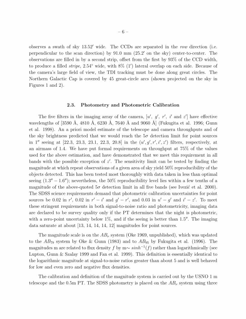
– 6 –

observes a swath of sky 13.52′ wide. The CCDs are separated in the row direction (i.e.

perpendicular to the scan direction) by 91.0 mm (25.2′ on the sky) center-to-center. The

observations are filled in by a second strip, offset from the first by 93% of the CCD width,

to produce a filled stripe, 2.54◦ wide, with 8% (1′) lateral overlap on each side. Because of

the camera’s large field of view, the TDI tracking must be done along great circles. The

Northern Galactic Cap is covered by 45 great-circle arcs (shown projected on the sky in

Figures 1 and 2).

2.3. Photometry and Photometric Calibration

The five filters in the imaging array of the camera, [u′, g′, r′, i′ and z′] have effective

wavelengths of [3590 A, 4810 A, 6230 A, 7640 A and 9060 A] (Fukugita et al. 1996; Gunn

et al. 1998). An a priori model estimate of the telescope and camera throughputs and of

the sky brightness predicted that we would reach the 5σ detection limit for point sources

in 1′′ seeing at [22.3, 23.3, 23.1, 22.3, 20.8] in the (u′, g′, r′, i′, z′) filters, respectively, at

an airmass of 1.4. We have put formal requirements on throughput at 75% of the values

used for the above estimation, and have demonstrated that we meet this requirement in all

bands with the possible exception of z′. The sensitivity limit can be tested by finding the

magnitude at which repeat observations of a given area of sky yield 50% reproducibility of the

objects detected. This has been tested most thoroughly with data taken in less than optimal

seeing (1.3′′ − 1.6′′); nevertheless, the 50% reproducibility level lies within a few tenths of a

magnitude of the above-quoted 5σ detection limit in all five bands (see Ivezic et al. 2000).

The SDSS science requirements demand that photometric calibration uncertainties for point

sources be 0.02 in r′, 0.02 in r′ − i′ and g′ − r′, and 0.03 in u′ − g′ and i′ − z′. To meet

these stringent requirements in both signal-to-noise ratio and photometricity, imaging data

are declared to be survey quality only if the PT determines that the night is photometric,

with a zero-point uncertainty below 1%, and if the seeing is better than 1.5′′. The imaging

data saturate at about [13, 14, 14, 14, 12] magnitudes for point sources.

The magnitude scale is on the ABν system (Oke 1969, unpublished), which was updated

to the AB79 system by Oke & Gunn (1983) and to AB95 by Fukugita et al. (1996). The

magnitudes m are related to flux density f by m∼ sinh−1(f) rather than logarithmically (see

Lupton, Gunn & Szalay 1999 and Fan et al. 1999). This definition is essentially identical to

the logarithmic magnitude at signal-to-noise ratios greater than about 5 and is well behaved

for low and even zero and negative flux densities.

The calibration and definition of the magnitude system is carried out by the USNO 1 m

telescope and the 0.5m PT. The SDSS photometry is placed on the ABν system using three

– 7 –

fundamental standards (BD + 17◦4708, BD + 26◦2606, and BD + 21◦609), whose magnitude

scale is as defined by Fukugita et al. (1996); a set of 157 primary standards, which are

calibrated by the above fundamental standards using the USNO 1m telescope, and which

cover the whole range of right ascension and enable the calibration system to be made

self-consistent; and a set of secondary calibration patches lying across the imaging stripes,

containing stars fainter than 14m whose magnitudes are calibrated by the PT with respect

to those of the primary standards and which transfer that calibration to the imaging survey.

The locations of these patches on the survey stripes are shown in Figure 1. On nights when

the 2.5 m is observing, the PT observes primary standard stars to provide the atmospheric

extinction coefficients over the night and to confirm that the night is photometric. The

standard star network is described in photcal/photcal.htm — note that the telescope

described there has now been replaced by the 0.5m PT.

2.4. Astrometric Calibration

The camera also contains leading and trailing astrometric arrays — narrow (128×2048),

neutral-density-filtered, r′-filtered CCDs covering the entire width of the camera. These

arrays can measure objects in the magnitude range r′ ∼ 8.5 - 16.8, i.e. they cover the dynamic

range between the standard astrometric catalog stars and the brightest unsaturated stars in

the photometric array. The astrometric calibration is thereby referenced to the fundamental

astrometric catalogues (see astrom/astrom.htm), using the Hipparcos and Tycho Catalogues

(ESA 1997) and specially observed equatorial fields (Stone et al. 1999). Comparison with

positions from the FIRST (Becker et al. 1995) and 2MASS (Skrutskie 1999) catalogues

shows that the rms astrometric accuracy is currently better than 150 milliarcseconds (mas)

in each coordinate.

2.5. Imaging Survey: North Galactic Cap

The imaging survey covers about 10,000 contiguous square degrees in the Northern

Galactic Cap. This area lies basically above Galactic latitude 30◦, but its footprint is adjusted

slightly to lie within the minimum of the Galactic extinction contours (Schlegel, Finkbeiner

& Davis 1998), resulting in an elliptical region. The region is centered at α = 12h 20m,

δ = +32.5◦. The minor axis is at an angle 20◦ East of North with extent ±55◦. The major

axis is a great circle perpendicular to the minor axis with extent ±65◦. The survey footprint

with the location of the stripes is shown in Figure 2 — see strategy/strategy.htm for

details.

– 8 –

2.6. Imaging Survey: The South Galactic Cap

In the South Galactic Cap, three stripes will be observed, one along the Celestial Equator

and the other two north and south of the equator (see Figure 2). The equatorial stripe (α

= 20.7h to 4h, δ = 0◦) will be observed repeatedly, both to find variable objects and, when

co-added, to reach magnitude limits about 2m deeper than the Northern imaging survey.

The other two stripes will cover great circles lying between α, δ of (20.7h, -5.8◦ → 4.0h,

-5.8◦) and (22.4h, 8.7◦ → 2.3h, 13.2◦).

2.7. The Spectroscopic Survey

Objects are detected in the imaging survey, classified as point source or extended, and

measured, by the image analysis software (see below). These imaging data are used to select

in a uniform way different classes of objects whose spectra will be taken. The final details of

this target selection will be described once the survey is well underway; the criteria discussed

here are likely to be very close to those finally used.

Two samples of galaxies are selected from the objects classified as “extended”. About

9 × 105 galaxies will be selected to have Petrosian (1976) magnitudes r′P ≤ 17.7. Galax-

ies with a mean r′ band surface brightness within the half light radius fainter than 24

magnitudes/arc second2 will be removed, since spectroscopic observations are unlikely to

produce a redshift. For illustrative purposes, a simulation of a slice of the SDSS redshift

survey is shown in Figure 3 (from Colley et al. 2000). Galaxies in this CDM simulation

are ‘selected’ by the SDSS selection criteria. As Figure 3 demonstrates, the SDSS volume is

large enough to contain a statistically significant sample of the largest structures predicted.

The second sample, of approximately 105 galaxies, exploits the characteristic very red

color and high metallicity (producing strong absorption lines) of the most luminous galaxies:

the “Brightest Cluster Galaxies” or “Bright Red Galaxies” (BRGs); redshifts can be well

measured with the SDSS spectra for these galaxies to about r′ = 19.5. Galaxies located

at the dynamical centers of nearby dense clusters often have these properties. Reasonably

accurate photometric redshifts (Connolly et al. 1995) can be determined for these galaxies,

allowing the selection by magnitude and g′r′i′ color of an essentially distance limited sample

of the highest-density regions of the Universe to a redshift of about 0.45 (see Figure 4 for a

simulation).

With their power-law continua and the influence of Lyman-α emission and the Lyman-α

forest, quasars have u′g′r′i′z′ colors quite distinct from those of the vastly more numerous

– 9 –

stars over most of their redshift range (Fan 1999). Thus about 1.5 × 105 quasar candidates

are selected for spectroscopic observations as outliers from the stellar locus (cf., Krisciunas

et al. 1998; Lenz et al. 1998; Newberg et al. 1999; Figure 5 below) in color-color space. At

the cost of some loss of efficiency, selection is allowed closer to the stellar locus around z =

2.8, where quasar colors approach those of early F and late A stars (Newberg & Yanny 1997;

Fan 1999). Some further regions of color-color space outside the main part of the stellar

locus where quasars are very rarely found are also excluded, including the regions containing

M dwarf-white dwarf pairs, early A stars, and white dwarfs (see Figure 5). The SDSS will

compile a sample of quasars brighter than i′ ≈ 19 at z < 3.0; at redshifts between 3.0 and

about 5.2, the limiting magnitude will be about i′ = 20. Objects are also required to be point

sources, except in the region of color-color space where low-redshift quasars are expected to

be found. Stellar objects brighter than i′ =20 which are FIRST sources (Becker, White and

Helfand 1995) are also selected. Based on early spectroscopy, we estimate that roughly 65%

of our quasar candidates are genuine quasars; comparison with samples of known quasars

indicates that our completeness is of order 90%.

In all cases, the magnitudes of the objects are corrected for Galactic extinction before

selection, using extinction in the SDSS bands calculated from the reddening map of Schlegel,

Finkbeiner & Davis (1998). Objects are then selected to have a magnitude limit outside the

Galaxy. If this correction were not made, the systematic effects of Galactic extinction over

the survey area would overwhelm the statistical uncertainties in the SDSS data set. After

the imaging and spectroscopic survey is completed in a given part of the sky, the reddening

and extinction will be recalculated using internal standards extracted from the imaging data.

The SDSS plans to use a variety of extinction probes, including very hot halo subdwarfs,

halo turnoff stars, and elliptical galaxies whose intrinsic colors can be estimated from their

line indices.

Together with various classes of calibration stars and fibers which observe blank sky to

measure the sky spectrum, the selected galaxies and quasars are mapped onto the sky, and

‘tiled’, i.e. their location on a 3◦ diameter plug plate determined (tiling/tiling.htm). The

centers of the tiles are adjusted to provide closer coverage of regions of high galactic surface

density, to make the spectroscopic coverage optimally uniform. Excess fibers are allocated to

several classes of rare or peculiar objects (for example objects which are positionally matched

with ROSAT sources, or those whose parameters lie outside any known range – these are

serendipitous objects) and to samples of stars. The spectra are observed, 640 at a time (with

a total integration time of 45 - 60 minutes depending on observing conditions) using a pair

of fiber-fed double spectrographs (spectro/spectro.htm). The wavelength coverage of the

spectrographs is continuous from about 3800 A to 9200 A, and the wavelength resolution,

λ/δλ, is 1800 (Uomoto et al. 1999). The fibers are located at the focal plane via plug

– 10 –

plates constructed for each area of sky. The fiber diameter is 0.2 mm (3′′ on the sky), and

adjacent fibers cannot be located more closely than 55′′ on the sky. Both members of a pair

of objects closer than this separation can be observed spectroscopically if they are located

in the overlapping regions of adjacent tiles.

Tests of the redshift accuracy using observations of stars in M67 whose radial velocities

are accurately known (Mathieu et al. 1986) show that the SDSS radial velocity measurements

for stars have a scatter of about 3.5 km s−1.

3. Software and Data Products

The operational software is described in datasys/datasys.htm. The data are obtained

using the Data Acquisition (DA) system at APO (Petravick et al. 1994) and recorded on DLT

tape. The imaging data consist of full images from all CCDs of the imaging array, cut-outs

of detected objects from the astrometric array, and bookkeeping information. These tapes

are shipped to Fermilab by express courier and the data are automatically reduced through

an interoperating set of software pipelines operating in a common computing environment.

The photometric pipeline reduces the imaging data; it corrects the data for data de-

fects (interpolation over bad columns and bleed trails, finding and interpolating over ‘cosmic

rays’, etc), calculates overscan (bias), sky and flat field values, calculates the point spread

functions (psf) as a function of time and location on the CCD array, finds objects, com-

bines the data from the five bands, carries out simple model fits to the images of each

object, deblends overlapping objects, and measures positions, magnitudes (including psf and

Petrosian magnitudes) and shape parameters. The photometric pipeline uses position cali-

bration information from the astrometric array reduced through the astrometric pipeline and

photometric calibration data from the photometric telescope (reduced through the photomet-

ric telescope pipeline). Final calibrations are applied by the final calibration pipeline, which

allows refinements in the positional and photometric calibration as the survey progresses.

The photometric pipeline is extensively tested using repeat observations, examination of the

outputs, observations of regions of the sky previously observed by other telescopes (HST

fields, for example) and a set of simulations, described in detail in simul/simul.htm. For

an example of the repeatability of SDSS photometry over several timescales, see Ivezic et al.

(2000). These repeat observations show that the mean errors (for point sources) are about

0.03m to 20m, increasing to about 0.05m at 21m and to 0.12m at 22m. These observed errors

are in good agreement with those quoted by the photometric pipeline. They apply only to

the g′, r′ and i′ bands – in the less sensitive u′ and z′ bands, the errors at the bright end are

about the same as those in g′r′i′, but increase to 0.05m at 20m and 0.12m at 21m.

– 11 –

The outputs, together with all the observing and processing information, are loaded

into the operational data base which is the central collection of scientific and bookkeeping

data used to run the survey. To select the spectroscopic targets, objects are run through

the target selection pipeline and flagged if they meet the spectroscopic selection criteria for

a particular type of object. The criteria for the primary objects (quasars, galaxies and

BRGs) will not be changed once the survey is underway. Those for serendipitous objects

and samples of interesting stars can be changed throughout the survey. A given object can in

principle receive several target flags. The selected objects are tiled as described above, plug

plates are drilled, and the spectroscopic observations are made. The spectroscopic data are

automatically reduced by the spectroscopic pipeline, which extracts, corrects and calibrates

the spectra, determines the spectral types, and measures the redshifts. The reduced spectra

are then stored in the operational data base. The contents of the operational data base are

copied at regular intervals into the science data base for retrieval and scientific analysis (see

appsoft/appsoft.htm). The science data base is indexed in a hierarchical manner: the

data and other information are linked into ‘containers’ that can be divided and subdivided

as necessary, to define easily searchable regions with approximately the same data content.

This hierarchical scheme is consistent with those being adopted by other large surveys, to

allow cross referencing of multiple surveys. The science data base also incorporates a set of

query tools and is designed for easy portability.

The photometric data products of the SDSS include: a catalog of all detected objects,

with measured positions, magnitudes, shape parameters, model fits and processing flags;

atlas images (i.e. cutouts from the imaging data in all five bands) of all detected objects

and of objects from the FIRST and ROSAT catalogs; a 4× 4 binned image of the corrected

images with the objects removed: and a mask of the areas of sky not processed (because of

saturated stars, for example) and of corrected pixels (e.g. those from which cosmic rays were

removed). The atlas images are sized to enclose the area occupied by each object plus the

PSF width, or the object size given in the ROSAT or FIRST catalogues. The photometric

outputs are described in http://www.astro.princeton.edu/SDSS/photo.html. The data

base will also contain the calibrated 1D spectra, the derived redshift and spectral type, and the

bookkeeping information related to the spectroscopic observations. In addition, the positions

of astrometric calibration stars measured by the astrometric pipeline and the magnitudes

of the faint photometric standards measured by the photometric telescope pipeline will be

published at regular intervals.

– 12 –

4. Early Science from the SDSS Commissioning Data

The goal of the SDSS is to provide the data necessary for studies of the large scale

structure of the Universe on a wide range of scales. The imaging survey should detect ∼ 5×

107 galaxies, ∼ 106 quasars and ∼ 8×107 stars to the survey limits. These photometric data,

via photometric redshifts and various statistical techniques such as the angular correlation

function, support studies of large scale structure well past the limit of the spectroscopic

survey. On even larger scales, information on structure will come from quasars.

The science justification for the SDSS is discussed in several conference papers (e.g.

Gunn & Weinberg 1995; Fukugita 1998; Margon 1999). The Project Book science sec-

tions can be accessed at http://www.astro.princeton.edu/PBOOK/science/science.htm.

Much of the science for which the SDSS was built, the study of large scale structure, will

come when the survey is complete, but the initial test data have already led to significant

scientific discoveries in many fields. In this section, we show examples of the first test data

and some initial results. To date (May 2000), the SDSS has obtained test imaging data for

some 2000 square degrees of sky and about 20,000 spectra. Examples of these data are shown

in Figures 5 (sample color-color and color-magnitude diagrams of point-source objects), 6

(sample spectra) and 7 (a composite color image of a piece of the sky which contains the

cluster Abell 267),

Fischer et al. (2000) have detected the signature of the weak lensing of background

galaxies by foreground galaxies, allowing the halos and total masses of the foreground galaxies

to be measured.

The searches by Fan et al. (1999a,b; 2000a,c), Schneider et al. (2000) and Zheng et

al. (2000) have greatly increased the number of known high redshift (z>3.6) quasars and

include several quasars with z > 5. Fan et al. (1999b) have found the first example of a new

kind of quasar: a high redshift object with a featureless spectrum and without the radio

emission and polarization characteristics of BL Lac objects. The redshift for this object (z

= 4.6) is found from the Lyman-α forest absorption in the spectrum.

Some 150 distant probable RR Lyrae stars have been found in the Galactic halo, enabling

the halo stellar density to be mapped; the distribution may have located the edge of the halo

at approximately 60 kpc (Ivezic et al. 2000). The distribution of RR Lyrae stars and other

horizontal branch stars is very clumped, showing the presence of possible tidal streamers in

the halo (Ivezic et al. 2000; Yanny et al. 2000). Margon et al. (1999) describe the discovery

of faint high latitude carbon stars in the SDSS data.

Strauss et al. (1999), Schneider et al. (2000), Fan et al. (2000b), Tsvetanov et al.

(2000), Pier et al. (2000) and Leggett et al. (2000) report the discovery of a number of

– 13 –

very low mass stars or substellar objects, those of type ‘L’ or ‘T’, including the first field

methane (‘T’) dwarfs and the first stars of spectral type intermediate between ‘L’ and ‘T’.

The detection rate to date shows that the SDSS is likely to identify several thousand L and

T dwarfs. These objects are found to occupy very distinct regions of color-color and color-

magnitude space, which will enable the completeness of the samples to be well characterized.

Measurements of the psf diameter variations and the image wander allow variations

in the turbulence in the Earth’s atmosphere to be tracked. These data demonstrate the

presence of anomalous refraction on scales at least as large as the 2.3◦ field of view of the

camera (Pier et al. 1999).

Of course the most exciting possibility for any large survey which probes new regions

of sensitivity or wavelength is the discovery of exceedingly rare or entirely new classes of

objects. The SDSS has already found a number of very unusual objects; the nature of some

of these remains unknown (Fan et al. 1999c). These and other investigations in progress

show the promise of SDSS for greatly advancing astronomical work in fields ranging from the

behavior of the Earth’s atmosphere to structure on the scale of the horizon of the Universe.

The Sloan Digital Sky Survey (SDSS) is a joint project of The University of Chicago,

Fermilab, the Institute for Advanced Study, the Japan Participation Group, The Johns Hop-

kins University, the Max-Planck-Institute for Astronomy, Princeton University, the United

States Naval Observatory, and the University of Washington. Apache Point Observatory,

site of the SDSS, is operated by the Astrophysical Research Consortium. Funding for the

project has been provided by the Alfred P. Sloan Foundation, the SDSS member institutions,

the National Aeronautics and Space Administration, the National Science Foundation, the

U.S. Department of Energy, and Monbusho. The official SDSS web site is www.sdss.org.

REFERENCES

Bade, N., Engels, D., Voges, W., et al. 1998, A&AS, 127, 145

Becker, R.H., White, R.L., & Helfand, D.J. 1995, ApJ, 450, 559

Berger, J., & Fringant, A.-M., 1985, A&AS, 61, 191

Colley, W. N., Gott, J. R., Weinberg, D. H., Park, C., & Berlind, A. A. 2000, ApJ, 529, 795

Connolly, A.J., Csabai, I., Szalay, A.S., Koo, D.C., Kron, R.G., & Munn, J.A. 1995, AJ,

110, 2655

Crawford, C.S., Allen, S.W., Ebeling, H., A.C., & Fabian, A.C. 1999, MNRAS, 306, 857

– 14 –

ESA 1997, The Hipparcos and Tycho Catalogues, ESA SP-1020

Fan, X. 1999, AJ, 117, 2528

Fan, X., Strauss, M. A., Schneider, D.P., et al. 1999a, AJ, 118, 1

Fan, X., Strauss, M.A., Gunn, J.E. et al. 1999b, ApJ 526, L57

Fan, X., Strauss, M.A., Schneider, D.P., Gunn, J.E., Lupton, R.L., Knapp, G.R., & Yanny,

B. 1999c, AAS, 73.15

Fan, X., Strauss, M. A., Schneider, D.P., et al. 2000a, AJ, 119, 1

Fan, X., Knapp, G.R., Strauss, M.A., et al. 2000b, AJ, 119, 928

Fan, X., White, R.L., Davis, M., et al. 2000c, submitted to AJ

Fischer, P., McKay, T., Sheldon, E. et al. 2000, submitted to AJ (astro-ph/9912119)

Fukugita, M. 1998, in Highlights of Astronomy, 11A, ed. J Andersen, 449.

Fukugita, M., Ichikawa, T., Gunn, J.E., Doi, M., Shimasaku, K., & Schneider, D.P. 1996,

AJ, 111, 1748

Gunn, J.E., Carr, M.A., Rockosi, C.M., Sekiguchi, M., et al. 1998, AJ, 116, 3040

Gunn, J.E., & Weinberg, D.H. 1995, in “Wide Field Spectroscopy and the Distant Universe”,

ed. S. Maddox & A. Aragon-Salamanca, World Scientific (Singapore), 3

Hull, C., Limmongkol, S., & Siegmund, W. 1994, Proc. S.P.I.E., 2199

Ivezic, Z., Goldston, J., Finlator, K., et al. 2000, AJ (in press: astro-ph/0004130)

Krisciunas, K., Margon, B., & Szkody, P. 1998, PASP, 110, 1342

Lenz, D.D., Newberg, H.J., Rosner, R., Richards, G.T., & Stoughton, C. 1998, ApJS, 119,

121

Lupton, R.H., Gunn, J.E., & Szalay, A. 1999, AJ, 118, 1406

Mathieu, R.D., Latham, D.W., Griffin, R.F., & Gunn, J.E. 1986, AJ, 92, 1100

Margon, B. 1999, Philosophical Transactions of the Royal Society of London A, 357, 93.

Margon, B., Anderson, S.F., Deutsch, E., & Harris, H. 1999, BAAS 195.8006

Morris, S.L., Weymann, R.J., Anderson, S.F., Hewett, P.C., Foltz, C.B., Chaffee, F.H.,

Francis, P.J., & MacAlpine, G.M. 1991, AJ, 102, 1627

Newberg, H.J., & Yanny, B. 1997, ApJS, 113, 89

Newberg, H.H., Richards, G.T., Richmond, M.W., & Fan, X. 1999, ApJS, 123, 377

Oke, J.B., & Gunn, J.E. 1983, ApJ, 266, 713

– 15 –

Petravick, D., et al. 1994, S.P.I.E., 2198, 935

Petrosian, V. 1976, ApJ, 209, L1

Pier, J.R., Leggett, S.K., Strauss, M.A., et al. 2000, in “From Giant Planets to Cool Stars”,

ed.C. Griffith & M. Marley, ASP Conf. Ser., in press

Pier, J.R., Munn, J.A., Hennessy, G.S., Hindsley, R.H., & Kent, S.M. 1999, AAS, 195, 81.04

Schlegel, D.J., Finkbeiner, D.P., & Davis, M. 1998, ApJ, 500, 525

Schneider, D.P., Hill, G.J., Fan, X., et al. 2000, PASP, 112, 6

Skrutskie, M.F. 1999, AAS, 195, 34.01

Strauss, M.A., Fan, X., Gunn, J.E., et al., 1999, ApJ, 522, L61

Stone, R.C., Pier, J.R., & Monet, D.G. 1999, AJ, 118, 2488

Tsvetanov, Z.I., Golimowski, D., Zheng, W., et al. 2000, ApJ, 513, L61

Uomoto, A., Smee, S., Rockosi, C., Burles, S., Pope, A., Friedman, S., Brinkmann, J., Gunn,

J.E., & Nichol, R, 1999, AAS, 195.87.01

Yanny, B., Newberg, H., Kent, S., et al. 2000, AJ (in press: astro-ph/0004128)

Zheng, W., Tsvetanov, Z.I., Schneider, D.P., et al. 2000, submitted to AJ (astro-ph/0005247)

This preprint was prepared with the AAS LATEX macros v4.0.

– 16 –

Figure 1. Projection on the sky of the northern SDSS survey area. The positions of the Yale

Bright Star Catalogue stars are shown. The largest symbols are stars of 0m and the smallest

stars of 5m – 7m. The secondary calibration patches are shown by squares.

– 17 –

Figure 2. Projection on the sky (Galactic coordinates) of the Northern and Southern SDSS

surveys. The lines show the individual stripes to be scanned by the imaging camera. These

are overlaid on the extinction contours of Schlegel, Finkbeiner and Davis (1998). The Survey

pole is marked by the ‘X’.

– 18 –

Figure 3. A six-degree wide slice of the Simulated Sloan Digital Sky Survey (from Colley et

al. 2000), showing about 1/20 of the survey.

– 19 –

Figure 4. Simulated redshift distribution in a 6◦ slice of the SDSS. Small dots: main galaxy

sample (cf. Figure 3). Large dots: the BRG sample, showing about 1/30 of the survey.

– 20 –

Figure 5. Color-color and color-magnitude plots of about 117,000 point sources brighter

than 21m at i∗ and detected at greater than 5σ in each band from 25 square degrees of SDSS

imaging data, reduced by the photometric pipeline (the i∗ designation is used for preliminary

SDSS photometry). The contours are drawn at intervals of 10% of the peak density of points.

The redder stars extend to fainter magnitudes than do the bluer stars, due to the i∗ limit.

– 21 –

Figure 6. Representative SDSS spectra taken from a single spectroscopic plate observed

on 4 October 1999 for a total of one hour of integration time, processed by the SDSS

spectroscopic pipeline. For display purposes, all spectra have been smoothed with a 3-pixel

boxcar function. All spectra show significant residuals due to the strong sky line at 5577A.

The objects depicted are: a. An r∗P = 18.00 galaxy; z = 0.1913. This object is slightly fainter

than the main galaxy target selection limit. Note the Hα/[N II] emission at ∼ 7800A, [OII]

emission at ∼ 4450A, and Ca II H and K absorption at ∼ 4700A. b. An r∗P = 19.41 galaxy,

z = 0.3735. This object is close to the photometric limit of the Bright Red Galaxy sample.

The H and K lines are particularly strong. c. A star-forming galaxy with r∗P = 16.88, at

z = 0.1582. d. A z = 0.3162 quasar, with r∗psf = 16.67. Note the unusual profile shape of the

Balmer lines. This quasar is LBQS 0004+0036 (Morris et al. 1991). e. A z = 2.575 quasar

with r∗psf = 19.04; note the resolution of the Lyman-α forest. This quasar was discovered by

Berger & Fringant (1985). f. A hot white dwarf, with r∗psf = 18.09.

– 22 –

Figure 7. A sample frame (13′×9′) from the SDSS imaging commissioning data. The image,

a color composite made from the g′, r′, and i′ data, shows a field containing the distant

cluster Abell 267 (α = 01h 52m 41.0s, δ = + 01◦ 00′ 24.7′′, redshift z = 0.23, Crawford

et al. 1999); this is the cluster of galaxies with yellow colors in the lower center of the

frame. The frame also contains, in the upper center, the nearby cluster RX J0153.2+0102,

estimated redshift ∼ 0.07 (Bade et al. 1998) (α = 01h 53m 15.15s, δ = + 01◦ 02′ 18.8′′).

The psf (optics plus seeing) was about 1.6′′. Right ascension increases from bottom to top

of the frame, declination from left to right.