The stability of dual-PSD based calibration system without

The stability of dual-PSD based calibration system without its relativelocation to 3D forming of carbon fiber

Chengzhi Su1, a *, Lei Zhong1, b, Chengyun Wang1, c,Huzaifa Khalid1, d, Fangchao Shao1

1College of Mechanical and Electric Engineering, Changchun University of Science and Technology,Jilin Changchun 130022, China

[email protected], [email protected], [email protected],[email protected]

Keywords: Carbon fiber, 3D forming robot, Calibration, Dual-PSD, Alignment, Lyapunov method

Abstract. The trajectory accuracy of the carbon fiber 3D forming robots is one of the key factors toensure the quality of forming. It is well known that carbon fiber 3D forming robots have highrepeatability but low accuracy. Compared to conventionally used calibration methods, dual-PSDbased methods provide a more efficient way to accurately calibrate the joint offsets of industrialrobots. But the stability of dual-PSD calibration system requires a strict proof in mathematics whenthe relationship between the robot base frame and the PSD frame is unknown. In this paper, byusing an adaptive algorithm based on Lyapunov function, we can estimate the unknown parametersonline without the parameters of the relationship. It is proved that the laser spots were stable to thedesired positions on the dual-PSD plane. The performance is confirmed by the simulations at last.The carbon fiber 3D forming robots positioning accuracy can reach 0.0222mm when the methodproposed in this paper is used successfully. In this case, the quality of the forming can be assured.

Introduction

Carbon fiber is a new type of industrial material and has been applied in many fields. The carbonfiber 3D forming robots can print various precise parts, so its’ accuracy is of critical importance.The high precision automatic calibration system is a hot research topic to improve the precision of3D forming robot localization. Dual-PSD based robot calibration system has been proposed inreference [1]. Due to that the position of the dual-PSD in the robot's task space is unknown, thestudy on the stability of the unknown system is the primary problem of the calibration method. Forthe study on the stability of robot system, models and control approaches based on dual-PSD havebeen proposed by Yunyi Jia, Chengzhi Su, et al. [2, 3] and the simulation experiments have beencarried out. Zhihui Deng, Yunyi Jia, et al. [4] have designed the dual-PSD based adaptive alignmentalgorithm and have given a conclusion that the system is stable by simulation. Yantao Shen,Guoliang Xiang, et al. [5] have adopted visual servo control on a planar robot when thetransformation matrix between the CCD camera frame and the robot base frame is unknown andhave proved the stability of the system by Lyapunov method. In literature [6], Yantao Shen, NingXi, et al. have proposed the adaptive algorithm when the position of the PSD array is unknown inthe robot task space, eventually have reached the conclusion that the laser spots were stable to thedesired positions. For the stability of the system, in the literature [2-4], the corresponding controlalgorithms have been proposed, and the simulation results have been demostrated, however, thetheoretical proof has not been discussed. In literature [5, 6], the discussion of the system stabilitywas only on planar robots. There is no theoretical proof about the stability of the space robotcalibration system based on dual-PSD. The Lyapunov function based adaptive estimation law isdesigned and the large scale asymptotic stability of the calibration method have been proved in thispaper, which lays a theoretical foundation for the study of the calibration system.

International Symposium on Mechanical Engineering and Material Science (ISMEMS 2016)

Copyright © 2016, the Authors. Published by Atlantis Press. This is an open access article under the CC BY-NC license (http://creativecommons.org/licenses/by-nc/4.0/).

Advances in Engineering Research, volume 93

444

The Dual PSD Calibration System Overview

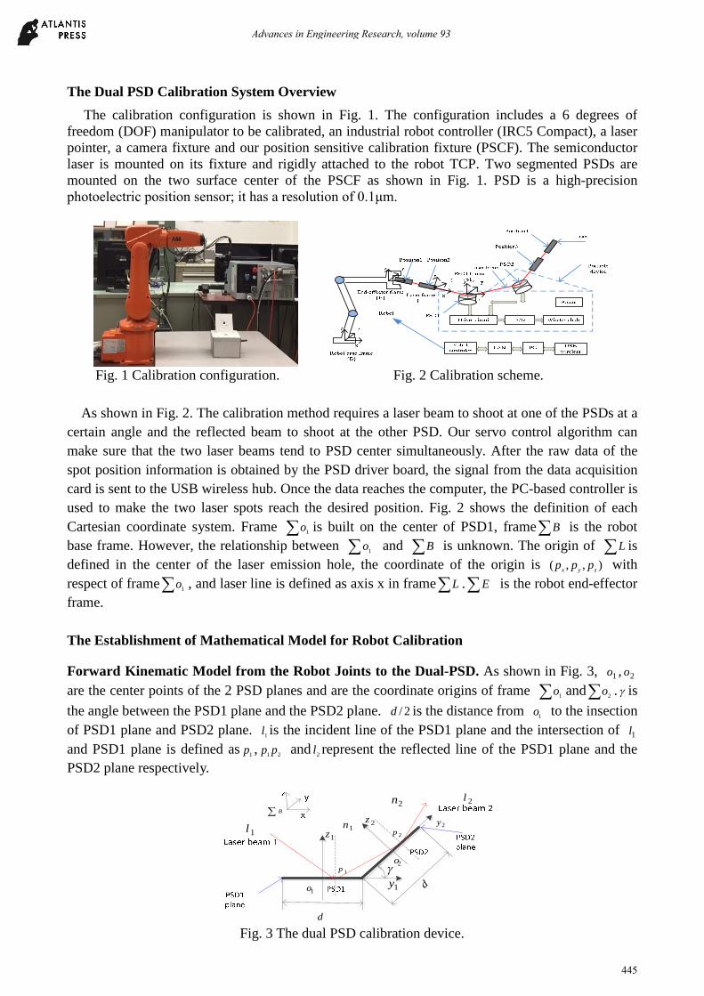
The calibration configuration is shown in Fig. 1. The configuration includes a 6 degrees offreedom (DOF) manipulator to be calibrated, an industrial robot controller (IRC5 Compact), a laserpointer, a camera fixture and our position sensitive calibration fixture (PSCF). The semiconductorlaser is mounted on its fixture and rigidly attached to the robot TCP. Two segmented PSDs aremounted on the two surface center of the PSCF as shown in Fig. 1. PSD is a high-precisionphotoelectric position sensor; it has a resolution of 0.1μm.

Fig. 1 Calibration configuration. Fig. 2 Calibration scheme.

As shown in Fig. 2. The calibration method requires a laser beam to shoot at one of the PSDs at a

certain angle and the reflected beam to shoot at the other PSD. Our servo control algorithm can

make sure that the two laser beams tend to PSD center simultaneously. After the raw data of the

spot position information is obtained by the PSD driver board, the signal from the data acquisition

card is sent to the USB wireless hub. Once the data reaches the computer, the PC-based controller is

used to make the two laser spots reach the desired position. Fig. 2 shows the definition of each

Cartesian coordinate system. Frame ∑ 1o is built on the center of PSD1, frame∑B is the robot

base frame. However, the relationship between ∑ 1o and ∑B is unknown. The origin of ∑L is

defined in the center of the laser emission hole, the coordinate of the origin is ),,( zyx ppp with

respect of frame∑ 1o , and laser line is defined as axis x in frame∑L .∑E is the robot end-effector

frame.

The Establishment of Mathematical Model for Robot Calibration

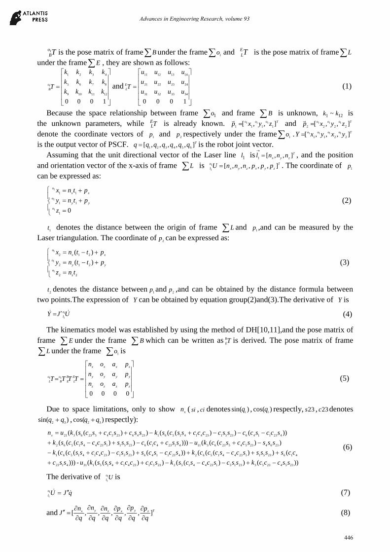
Forward Kinematic Model from the Robot Joints to the Dual-PSD. As shown in Fig. 3, 1o , 2o

are the center points of the 2 PSD planes and are the coordinate origins of frame ∑ 1o and∑ 2o . γ is

the angle between the PSD1 plane and the PSD2 plane. 2/d is the distance from1

o to the insection

of PSD1 plane and PSD2 plane.1

l is the incident line of the PSD1 plane and the intersection of 1l

and PSD1 plane is defined as1

p ,21

pp and2

l represent the reflected line of the PSD1 plane and the

PSD2 plane respectively.

1o

2o

1y

1z2z

2y1n

2n

γ

1l

2l

∑ B

d

d

1p

2p

Fig. 3 The dual PSD calibration device.


445

ToB1 is the pose matrix of frame∑B under the frame∑ 1o and TE

L is the pose matrix of frame∑L

under the frame∑E , they are shown as follows:

=

1000

1211109

8765

4321

1

kkkk

kkkk

kkkk

To

Band

=

1000

34333231

24232221

14131211

uuuu

uuuu

uuuu

TE

L(1)

Because the space relationship between frame ∑ 1o and frame ∑B is unknown, 121 ~ kk is

the unknown parameters, while TEL is already known. Tooo zyxp ],,[

1111111=

rand Tooo zyxp ],,[

2222111=

r

denote the coordinate vectors of1

p and2

p respectively under the frame∑ 1o . Toooo yxyxY ],,,[2211

1111=

is the output vector of PSCF. Tqqqqqqq ],,,,,[654321

= is the robot joint vector.

Assuming that the unit directional vector of the Laser line 1l is T

zyxnnnl ],,[

1=

→

, and the position

and orientation vector of the x-axis of frame ∑L is T

zyxzyx

o

l pppnnnU ],,,,,[1

1= . The coordinate of

1p

can be expressed as:

=

+=

+=

01

11

11

1

1

1

z

ptny

ptnx

o

yy

o

xx

o

(2)

1t denotes the distance between the origin of frame ∑L and

1p ,and can be measured by the

Laser triangulation. The coordinate of2

p can be expressed as:

=

+−=

+−=

22

212

212

1

1

1

)(

)(

tnz

pttny

pttnx

z

o

yy

o

xx

o

(3)

2t denotes the distance between

1p and

2p ,and can be obtained by the distance formula between

two points.The expression of Y can be obtained by equation group(2)and(3).The derivative of Y is

UJY o

l&& 1

1′= (4)

The kinematics model was established by using the method of DH[10,11],and the pose matrix of

frame ∑E under the frame ∑B which can be written as TB

E is derived. The pose matrix of frame

∑L under the frame ∑ 1o is

==

0000

11

zzzz

yyyy

xxxx

E

L

B

E

o

B

o

Lpaon

paon

paon

TTTT (5)

Due to space limitations, only to show xn ( si , ci denotes )sin(

iq , )cos(

iq respectly, 23s , 23c denotes

)sin(32

qq + , )cos(32

qq + respectly):

))())(())(((-)))

())((())())(((

))((()))())(((

))())((())(((

23542353231512344152235123414151314123

416235112344156242311462351234141561

23642354523631141234162351123441562

42311462351234141561234623545236321

sscccksscsccscskscccccssskussc

ccsssssccscccksccscsssccccsscck

ssssccscckussccccssssccsccsk

sccsccssccccsscsksscsccscskunx

−+−−−+++

++−+−+−+−

−+−+−+−+

−−−+−++=

(6)

The derivative of Uo

l1

1is

qJUo

l&& ′′=1

1(7)

and Tzyxzyx

q

p

q

p

q

p

q

n

q

n

q

nJ ],,,,,[

∂

∂

∂

∂

∂

∂

∂

∂

∂

∂

∂

∂=′′ (8)


446

Combining Eq. (4) and (7), the forward kinematics model from the robot joints to the dual-PSDis derived:

qJJqJY &&& ′′⋅′== (9)

The unknown parameters of the formula (9) are placed in the 12×1 column vectorθ , so that theknown partial and unknown parameters are completely separated. That is

θ1DqJY == && (10)

Robotic Dynamic Model. The dynamic model of the robot with 6 degrees of freedom is estimated

using Newton-Euler method; it follows the robot dynamics equation:

τ=++ )(),()( qGqqqCqqH &&&& (11)

where, )(qH is the symmetric and positive definite inertia matrix. ),( qqC & denotes a skew-symmetric

matrix. )(qG is the gravity force. The τ represents the joint input of the manipulator.

The Proof of Asymptotic Stability based on the Lyapunov Equation

The Establishment of the Lyapunov Equation. In order to prove that the laser spots tend to the

desired positions on the double PSD plane, the Lyapunov function is defined based on energy

method:

})({2

11

YKYBqqHqVp

TTT ∆∆+∆∆+∆∆= θθ&& (12)

1B ,

pK is positive constant, θ is an estimated value of θ and θθθ ˆ−=∆ ; dqqq −=∆ represents

the joint vector errors;d

Y represents the desired positions, dYYY −=∆ represents the position errors of

laser spots, at this point YY && =∆ ;also, we have qq && =∆ .

The derivative of Eq. (12) is:

YKYBqHqqHqVp

TTTT ∆∆+∆∆++= &&&&&&&&& θθ1

2

1(13)

According to the characteristics of robot dynamics, CH 2−& is skew-symmetric matrix, namelyCH 2=& , so we have:

θθ

θθ

&&&&&&

&&&&&&&&&

∆∆+∆++=

∆+∆∆++=

1

1

]),([

)(),(

BYJKqqqCqHq

YKqJBqqqCqqHqV

TT

p

T

p

TTTT

(14)

Combining (11) we have: θθτ &&& ∆∆+∆+−=1

])([ BYJKqGqV TT

p

T (15)

The Design of Adaptive Control Law. The control problem belongs to the fixed point control, we

can adopt PD plus gravity compensation algorithm to design the adaptive control law:

YJKqKqG T

pv∆−−= ˆ)( &τ (16)

vK is the positive constant, TJ represents the estimated matrix of TJ .Substituting the adaptive

control law (16) into the robot dynamics Eq. (11), closed-loop dynamics equation is derived:

YJKqKqqqCqqH T

pv∆−−=+ ˆ),()( &&&&& (17)

The error between the real and the estimated value of the spot speeds:

θ∆=−=−1

)ˆ(ˆ DqJJYY &&& (18)

The Design of Adaptive Parameter Estimation Law. Substituting the designed control law (16)

into Eq. (15), and combining Eq. (10), we can derive that


447

θθθ &&&& ∆∆+∆∆+−=11

BYDKqKqV TTT

pv

T (19)

To get a stable system and make q& and θ∆ asymptotically stable to the desired value, an

adaptively estimated law is designed as

θθθθθ ∆∆−=∆∆+∆∆2111

BBBYDK TTTT

p& (20)

2B is a positive constant. Simplifying Eq. (20), the adaptively estimated law can be written as:

YDB

KB

dt

d Tp∆∆=

∆1

1

2 -- θθ

(21)

The Proof of Asymptotic Convergence. The expression (21) is first order differential equation

group with constant coefficients，set YDB

Kta Tp ∆−= 1

1

)( , then the solution of the equation group is:

ττθθ τ daeet

tAAt )(0

)(

0 ∫−+∆=∆ (22)

0θ∆ is the initial value of θ∆ , 12122 ×

−= EBA , 1212×E is 12 order unit matrix. When ∞→t , in

expression (22), 00→∆θAte ;so

200

)( )(lim)(lim)(limlim

B

tadaeedae

t

tAAt

t

ttA

tt ∞→

−

∞→

−

∞→∞→===∆ ∫∫ ττττθ ττ (23)

The stability condition of estimation law: we can see from formula (10) that when 0=q& , each

element of matrix 1D equals0, namely 0)( =ta , at this point θ∆ asymptotically stable to 0.

Substituting Eq. (20) into Eq. (19),we can get:

θθ ∆∆−= 21- BBqKqV T

v

T &&& (24)

It is proved that there are global positive-definite Lyapunov function V , the differential of

which is nonpositive. Set 0≡V& , at this point, 0≡q& , 0≡∆θ and only the zero solution satisfies the

equation. According to LaSalle theorem, 0=q& is asymptotically stable, namely each element of

matrix 1D asymptotically stable to 0, so θ is bounded; so the derived stable value of q& and θ∆

is consistent with the stability condition of estimation law we have obtained. Combining Eq. (16),

the conclusion is reached that the laser spot position error Y∆ on dual-PSD plane asymptotically

stable to 0 when time tends to infinity.

Simulation Experiments

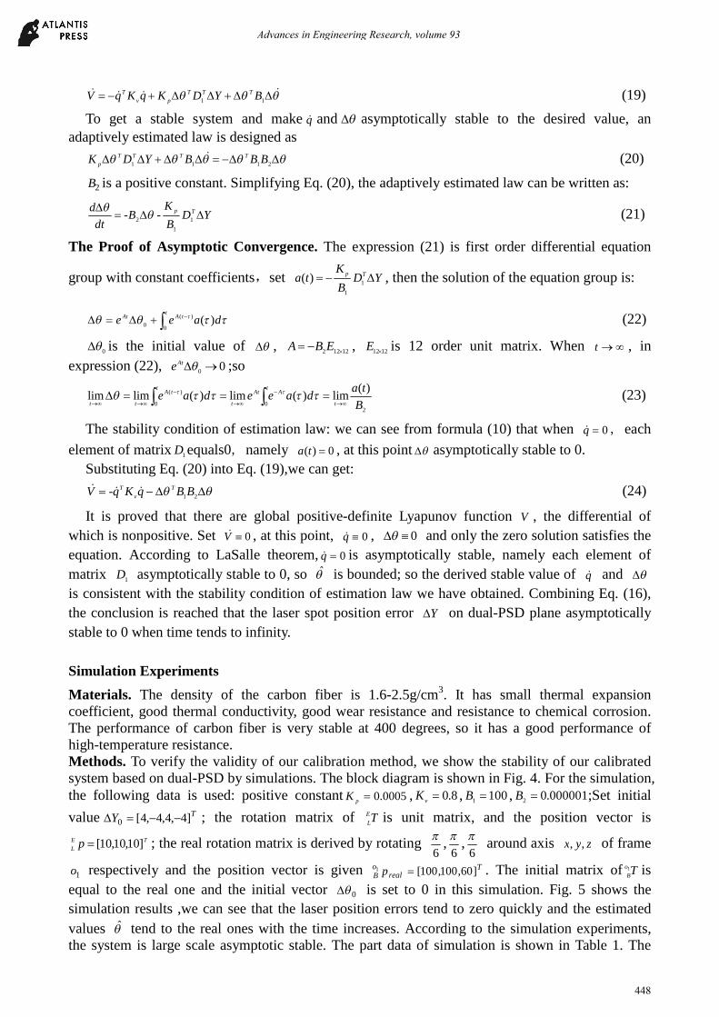
Materials. The density of the carbon fiber is 1.6-2.5g/cm3. It has small thermal expansioncoefficient, good thermal conductivity, good wear resistance and resistance to chemical corrosion.The performance of carbon fiber is very stable at 400 degrees, so it has a good performance ofhigh-temperature resistance.Methods. To verify the validity of our calibration method, we show the stability of our calibratedsystem based on dual-PSD by simulations. The block diagram is shown in Fig. 4. For the simulation,the following data is used: positive constant 0005.0=pK , 8.0=

vK , 100

1=B , 000001.0

2=B ;Set initial

value TY ]4,4,4,4[0 −−=∆ ; the rotation matrix of TE

L is unit matrix, and the position vector is

TE

Lp ]10,10,10[= ; the real rotation matrix is derived by rotating

6

π,

6

π,

6

πaround axis zyx ,, of frame

1o respectively and the position vector is given Treal

oB p ]60,100,100[1 = . The initial matrix of To

B1 is

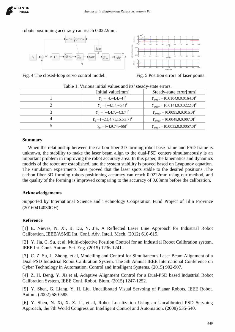
equal to the real one and the initial vector 0θ∆ is set to 0 in this simulation. Fig. 5 shows the

simulation results ,we can see that the laser position errors tend to zero quickly and the estimated

values θ tend to the real ones with the time increases. According to the simulation experiments,the system is large scale asymptotic stable. The part data of simulation is shown in Table 1. The


448

robots positioning accuracy can reach 0.0222mm.

1−JdY Y∆esti

boT

1 realo

bT1

Y0qq +∫ dt&

τθθ τ YdDeB

Ke T

ttApAt ∆−∆=∆ ∫−

10

)(

1

0

Robot )(qfY =dY

ikine

Fig. 4 The closed-loop servo control model. Fig. 5 Position errors of laser points.

Table 1. Various initial values and its’ steady-state errors.Initial value[mm] Steady-state error[mm]

1 TY ]4,4,4,4[0 −−= TerrorY ]0,0164.0,0,0104.0[=

2 TY ]4,5,4,1.4[0 −−= TerrorY ]0,0222.0,0,0141.0[=

3 TY ]7.3,4,7.4,4[0 −−= TerrorY ]0,015.0,0,0095.0[=

4 TY ]7.3,5.15,75.4,1.2[0 −= TerrorY ]0,007.0,0,0048.0[=

5 TY ]66,74,9,1[0 −−= TerrorY ]0,0057.0,0,0032.0[=

Summary

When the relationship between the carbon fiber 3D forming robot base frame and PSD frame isunknown, the stability to make the laser beam align to the dual-PSD centers simultaneously is animportant problem in improving the robot accuracy area. In this paper, the kinematics and dynamicsmodels of the robot are established, and the system stability is proved based on Lyapunov equation.The simulation experiments have proved that the laser spots stable to the desired positions .Thecarbon fiber 3D forming robots positioning accuracy can reach 0.0222mm using our method, andthe quality of the forming is improved comparing to the accuracy of 0.08mm before the calibration.

Acknowledgements

Supported by International Science and Technology Cooperation Fund Project of Jilin Province

(20160414030GH)

Reference

[1] E. Nieves, N. Xi, B. Du, Y. Jia, A Reflected Laser Line Approach for Industrial RobotCalibration, IEEE/ASME Int. Conf. Adv. Intell. Mech. (2012) 610-615.

[2] Y. Jia, C. Su, et al. Multi-objective Position Control for an Industrial Robot Calibration system,IEEE Int. Conf. Autom. Sci. Eng. (2015) 1236-1241.

[3] C. Z. Su, L. Zhong, et al, Modelling and Control for Simultaneous Laser Beam Alignment of aDual-PSD Industrial Robot Calibration System. The 5th Annual IEEE International Conference onCyber Technology in Automation, Control and Intelligent Systems. (2015) 902-907.

[4] Z. H. Deng, Y. Jia.et al, Adaptive Alignment Control for a Dual-PSD based Industrial RobotCalibration System, IEEE Conf. Robot. Biom. (2015) 1247-1252.

[5] Y. Shen, G. Liang, Y. H. Liu, Uncalibrated Visual Servoing of Planar Robots, IEEE Robot.Autom. (2002) 580-585.

[6] Y. Shen, N. Xi, X. Z. Li, et al, Robot Localization Using an Uncalibrated PSD ServoingApproach, the 7th World Congress on Intelligent Control and Automation. (2008) 535-540.

0 10 20 30 40 50 60 70 80 90 100-5

0

5x 10

-4

time(s)

deltath

eta

0 10 20 30 40 50 60 70 80 90 100-100

0

100

time(s)estimate

dvalue

ofth

eta

0 10 20 30 40 50 60 70 80 90 100-5

0

5

times(s)

delta

Y


449

Documents

The stability of dual-PSD based calibration system without