Eleventh Floor, Menzies Building Monash University, Wellington Road CLAYTON Vic 3800 AUSTRALIA Telephone: from overseas: (03) 9905 2398, (03) 9905 5112 61 3 9905 2398 or 61 3 9905 5112 Fax: (03) 9905 2426 61 3 9905 2426 e-mail: impact@buseco.monash.edu.au Internet home page: http//www.monash.edu.au/policy/

The Sydney Olympics, Seven Years On: An Ex-Post Dynamic CGE Assessment

by

JAMES GIESECKE and

JOHN MADDEN

Centre of Policy Studies Monash University

General Paper No. G-168 September 2007

ISSN 1 031 9034 ISBN 0 7326 1575 5

The Centre of Policy Studies (COPS) is a research centre at Monash University devoted to quantitative analysis of issues relevant to Australian economic policy.

i 

 

Contents Abstract 1

1. Introduction 1 2. Historical modelling to uncover the legacy of the Games 3 3. The Olympic simulations 6 4. The Olympic economic impact: simulation results 8

4.1 Foreign tourism 8 4.2 Interstate tourism 8 4.3 Construction and financing 9 4.4 Olympic Operations 9

5. Conclusions 10

References 22

Tables and Figures Table 1: Australian Macroeconomic Variables, Foreign Tourism Only 12 Table 2: State GDP Outcomes, Foreign Tourism Only 12 Table 3: NSW Macroeconomic Variables, Foreign Tourism Only 12 Table 4: National Industry Outputs, Foreign Tourism Only 13 Table 5: NSW Industry Outputs, Foreign Tourism Only 13 Table 6: Australian Macroeconomic Variables, Interstate Tourism Only 14 Table 7: State GDP Outcomes, Interstate Tourism Only 14 Table 8: NSW Macroeconomic Variables, Interstate Tourism Only 14 Table 9: National Industry Outputs, Interstate Tourism Only 15 Table 10: NSW Industry Outputs, Interstate Tourism Only 15 Table 11: Australian Macroeconomic Variables, Construction and Financing Only 16 Table 12: State GDP Outcomes, Construction and Financing Only 16 Table 13: NSW Macroeconomic Variables, Construction and Financing Only 16 Table 14: National Industry Outputs, Construction and Financing Only 17 Table 15: NSW Industry Outputs, Construction and Financing Only 17 Table 16: Australian Macroeconomic Variables, Operations Only 18 Table 17: State GDP Outcomes, Operations Only 18 Table 18: NSW Macroeconomic Variables, Operations Only 18 Table 19: National Industry Outputs, Operations Only 19 Table 20: NSW Industry Outputs, Operations Only 19 Table 21: Australian Macroeconomic Variables, Total 20 Table 22: State GDP Outcomes, Total 20 Table 23: NSW Macroeconomic Variables, Total 20 Table 24: National Industry Outputs, Total 21 Table 25: NSW Industry Outputs, Total 21 Figure 1: Foreign willingness to pay for Australian tourism 6 Figure 2: Olympics-related Direct Expenditure 7

i 

 

1

The Sydney Olympics, seven years on: an ex-post dynamic CGE assessment James A Giesecke1, John R Madden2

1 Centre of Policy Studies, Monash University, Clayton, Victoria, 3800,

james.giesecke@buseco.monash.edu.au 2 Centre of Policy Studies, Monash University, Clayton, Victoria, 3800,

john.madden@buseco.monash.edu.au

Abstract A recent development in ex-ante analysis of mega events is the use of computable general equilibrium (CGE) models. CGE models improve greatly on the input-output model, which they have largely displaced, since they incorporate fixed factors and substitution effects. However, like input-output, the method is still subject to the risk of over-optimistic estimation of benefits. We see three sources of such risk: (i) failure to treat public inputs as costs; (ii) elastic factor supply assumptions; and (iii) overestimation of foreign demand shocks via inclusion of “induced tourism” expenditure. In this paper, we undertake an ex-post analysis of the Olympics that addresses each of these risks. We handle the first two directly: public services used to support the Games (such as security services) are treated as Games-specific inputs, and we model the national labour market in full employment. For the third risk, we undertake an historical simulation to uncover the extent, if any, of induced tourism. We find no evidence of an induced tourism effect, and so exclude it from our analysis. With these assumptions, we find the Sydney Olympics generated a net consumption loss of approximately $2.1 billion.

Key words: Olympics economic impact, major projects, regional dynamic CGE. JEL Classification: R13, H43, C68.

1. Introduction

Over the past decade or two it has become commonplace for Olympic Games bids to be backed up by an economic impact study, generally aimed at highlighting the economic stimulus from the Games, as a counter to what appears to be an increasingly costly exercise. Kasimati (2003) reviews 13 studies which estimate the economic impact of Summer Olympic Games. All but one of these are ex-ante studies, with input-output (I/O) being the main vehicle of analysis. Typically, ex-ante economic impact studies project large impacts for mega-events (see Table 1 of Matheson, 2006)1.

However, such ex-ante studies have been subject to considerable criticism in the sports economics literature (see Porter, 199, Baade and Matheson, 2002, Owen, 2005 and Matheson, 2006). This is in line with a common criticism of ex-ante economic impact studies of sports operations (events, facilities and franchises) in general. As Coates & Humphreys (2003, p. 336) note, such economic impact studies are “prospective studies”. They need to be compared with “retrospective econometric studies”, which as Coates & Humphreys point out, tell quite a different story. Porter (1999, p. 61) states that “the projected spending and spillover benefits of regional impact models never materialize”. Indeed, as Siegfried & Zimbalist (2000, p.103) note, there is remarkable uniformity in the econometric results (of which they cite seven) that find no statistically significant evidence that constructing sports facilities generates economic development. Crompton (1995) discusses 11 typical problems 1 Estimated GDP impacts in the billions of dollars are not untypical for an Olympics Games or a Soccer World Cup.

2

with ex-ante studies of sports facilities and events. These problems range from incorrect use of the I/O method or misrepresentation of its results, through to omission of substitution effects and opportunity costs. Porter (1999) also lists some common errors in the use of I/O analysis. He considers there are systematic errors that lead to an overestimation of economic impacts. He undertook regression analysis of a number of mega events (Super Bowls) and found little impact on real sales in the host counties.

Some of the problems associated with ex-ante impact studies have been overcome in recent computable general equilibrium (CGE) impact studies of the Olympics and other mega sporting events. Examples are studies of the Sydney Olympics (Madden, 2002 and 2006), the London Olympics (Blake, 2005) and the Melbourne Commonwealth Games (KPMG, 2006). One advantage of a CGE model is that it automatically handles many of the displacement effects that arise from sports-related spending2. However, ex-ante CGE studies still face a number of problems. Even when such studies are conducted close enough to the Games so that the cost of staging the Games are reasonably well-known and revenue from TV rights, tickets, etc can be gauged with some degree of accuracy, the modeller still must make assumptions regarding certain factors which are likely to be key drivers of the results. Madden (2006) demonstrates that the estimated effects of the Sydney Games are very responsive to two factors. The first is the degree of induced tourism arising from the Games3. The second is the assumed degree of labour market responsiveness. Madden (2006) conducted sensitivity analysis and found large variations in the results. His standard scenario assumes induced tourism expenditure of just over 2.7 billion Australian dollars (1996 prices) and some degree of slackness in the labour market4. Under this standard scenario the present values (in 1996) of the impacts on Australian real consumption and real GDP were $2.5 billion and $6.5 billion respectively. However, if the assumed induced tourism is halved, these estimated effects are reduced to $1.4 billion and $4.9 billion respectively. Another scenario assumed the higher induced tourism, but assumed a very much tighter labour market5. Under this scenario the impacts on national real consumption and GDP are -$28 million and $1.5 billion respectively. Thus, under one very plausible assumption, we see that the impact on national real consumption (which, as Madden (2006) is at pains to point out, is the relevant variable for welfare analysis purposes) can be negative6. Indeed the effect on welfare (public and private real consumption) computed under this scenario is considerably negative, since an estimated $600 million in government expenditure is diverted to operating the Games. Of course, this does not mean that Australian households suffered a contraction in 2 Failure to incorporate such displacement effects is often pointed to (for instance, by Coates & Humphreys 2003, and by Matheson & Baade 2004) as a source of overly-optimistic estimates. CGE models, however, handle displacement effects by households by modelling their choice of goods as income constrained. Similarly, resource scarcities are taken into account by CGE models, so that some of the resources spent on the event and event-related activities (including associated tourism) are drawn from uses in other activities. Furthermore, the economic modeller is able to set up model simulations, in which governments neutralise the effect the event has on their own budgetary position, and, in the case of a national government, on the country’s external debt. 3 Induced-tourism expenditure (in Sydney and other Australian destinations) was included as a direct expenditure shock in the analysis of the Sydney Olympics. It was assumed that there would be generated by heightened international awareness of Australia by mechanisms (principally international media coverage of the Games and pre-Games stories) not present in the MMRF model. 4 Both Madden (2004) and Madden (2006) use the results from CREA/Arthur Andersen (1999) of which Madden was the author. Madden was also the author, together with Matt Crowe, of CREA/NSW Treasury (1997). 5 Under the standard scenario, one-quarter of the Olympics-induced labour demand acts to increase employment and the other three-quarters acts to increase real wages. Under the tighter labour-market scenario, only 5 per cent of the extra labour demand acts to increase national employment. 6 Most of the increase in GDP from the expenditure side is in sporting stadiums and the like which are assumed to have no value after the Games (an assumption which post-Games operating losses indicate mirrors reality).

3

economic welfare as a result of the Games, since there is likely to be other significant positive effects on welfare from an Olympic Games such as national-pride benefits, consumer surplus on Games tickets, better TV watching times, etc. Atkinson, et al. (2005), estimate, via contingency evaluation, that Britons would be willing to pay £2 billion for the intangible benefits associated with hosting the 2012 Games in London.

Thus, ex-ante results are subject to a good deal of uncertainty. In this paper we take up the question of whether we can use CGE modelling to make a more accurate estimate after the Games. A survey of the effects of the Sydney Olympics on foreign attitudes to Australia (Rivenburgh, 2004) casts some doubt as to how successful the Games might have been in inducing an increase in inbound tourism. There are no statistics available that directly show the degree of Games-induced tourism. To overcome this we turn to recent advances in dynamic CGE models that allow historical modelling to be undertaken. We demonstrate in this paper how we use historical modelling to uncover the movement in export demand curves in New South Wales and the rest of Australia in the relevant period. We are thus able to re-run our Olympics simulation with an induced tourism shock that is based on an estimate from historical data.

In the next section we provide an overview of our CGE model, historical modelling and the key results from our historical modelling exercise. We then discuss our approach to modelling the Olympics, before reporting the simulation results for the Olympics.

2. Historical modelling to uncover the legacy of the Games

The MMRF model in Brief MMRF models the behaviour of the key economic agents in eight regions of Australia –

the six states and two territories. In each region there are 15 industries, a representative household, importers and exporters, and a regional government. The model also has a federal government which interacts with economic agents in each region. Production by industries, consumption by householders, and investment are modelled in accordance with conventional economic theory. The eight regions are linked via interstate movements of commodities and factors of production (particularly labour).

Readers interested in a detailed description of MMRF should consult Adams, et al (2003). For a briefer overview, see Adams et al. (2000)7. Here we note just a few features of the model’s theory relevant to the present discussion.

MMRF treats producers as operating in a competitive market. Producers choose their inputs so as to minimize the costs of producing a particular quantity of output, subject to a given production technology. Substitution is allowed between commodity inputs from different geographical sources, and between labour, capital and land. If there is no change in relative prices, producers will vary their inputs in direct proportion to their output. However if a particular input becomes relatively expensive compared to substitutable inputs, producers will substitute towards the cheaper inputs.

Consumers in MMRF are also assumed to be optimising agents. They choose goods according to their preference pattern and relative prices, but are constrained by their amount of disposable income. If consumers switch their preferences towards attending a mega event, then in the absence of any increase in their income that might result from the event, they will reduce their spending on other goods. 7 The above references are for the dynamic version of MMRF. For an extended overview of the original model with only minimal dynamics, see Naqvi & Peter (1996).

4

MMRF provides results for economic variables on a year-on-year basis. It employs dynamic properties that have been styled on the national CGE model MONASH (Dixon and Rimmer, 2002). It is a recursive-dynamic multiregional CGE model, linking a sequence of single-period equilibria via stock-flow relationships. The equilibria thus computed change through time as the values for the model's stock variables change. Flows in previous periods (such as investment, inter-regional migration, and government borrowings) influence the values for the endogenous variables computed in each period through their contribution to the values of the model's stock variables (such as capital, population, and government debt) in each period.

Historical modelling A feature of MMRF, like its national counterpart MONASH, is its capacity for

sophisticated closure options. There are four major closure options that allow MONASH-style models to be run in four modes: historical, decomposition, forecasting and policy deviation. Our interest in this paper is the closure for the historical and policy modes, which we briefly outline below8:

Historical mode – is used to uncover the movement in certain unobservable variables during a period of (recent) history. This requires a closure that is very different from that normally employed in CGE models. Various variables (such as: real private consumption by commodity; real investment; output, employment and capital usage by industry; commodity exports and imports) that are normally endogenous, are reassigned to the exogenous category and shocked by historical values recorded in statistical sources. Corresponding normally-exogenous variables (such as: shifts in household preferences; investment/capital ratios; various technical change variables; shifts in foreign demand curves and domestic/import preferences) are swapped to the endogenous category.

Policy-deviation mode – In general, this mode is used for a forecast period (see Giesecke and Madden, 2007), but it can also be used to examine the effects of an historical period. The closure is changed to one suitable for modelling the particular policy scenario under consideration. Thus macroeconomic variables are reassigned to the endogenous category and the corresponding macroeconomic structural variables swapped into the exogenous category are shocked with their results from the historical simulation. The results deviate from the baseline, however, by the imposition of the policy shock under examination. This deviation gives the effect of implementing the policy.

The Olympics’ tourism legacy In the sports economics literature an induced tourism effect is often listed as a possible

legacy of a mega-event. In previous modelling of the Sydney Games this “legacy” is assumed to build up from the time of the announcement that Sydney would be the year 2000 host city, building to a peak the year after the Games, then falling away over the next four years until the effect disappears in 2006/07.

We now undertake an historical simulation to help uncover the extent of this “legacy”. That is, the historical simulations are used to elucidate the extent to which observed changes in tourism and sports related exports are due to the Games, and the extent to which they are due to unrelated factors, such as movements in national and regional real exchange rates.

8 Readers interested in decomposition and forecast closures should consult Dixon and Rimmer (2002) or Giesecke and Madden (2007).

5

As foreshadowed in the previous section, we exogenously determine macroeconomic variables for each state at their observed values, allowing the model to endogenously determine values for relevant structural variables. The key closure swaps are as follows. Real investment at the state level is determined exogenously via the endogenous determination of the positions of schedules linking investment at the regional industry level with rates of return. Private consumption spending in each state is determined exogenously via endogenous determination of region-specific average propensities to consume. Regional consumption spending by state and federal governments is naturally exogenous. Volumes of foreign imports into each region are determined exogenously via endogenous determination of region-specific import preference twists. State export volumes are exogenously determined via endogenous determination of primary factor technical change by state. Real state GDP is determined exogenously via endogenous determination of inter-regional sourcing preference twists. For the present simulation, the most important aspect of the historical closure relates to international visitor arrivals. We determine international visitor arrivals to each state exogenously at historically observed values by endogenously determining vertical positions of state-specific foreign tourism demand schedules. We conjecture that evidence of an induced visitor effect should be apparent in the revealed shifts in foreign willingness to pay for NSW and Australian tourism exports.

Figure 1 reports results for the vertical positions (willingness to pay shifts) of foreign demands for NSW tourism exports. For comparison, we also report the export-value weighted average of all states. The Australian average shows an upward trend over the study period, consistent with rapidly rising incomes in Australia’s foreign tourist origin countries. Dips attributable to the Asian financial crisis (1998/99), SARS and terrorist attacks in the US (2001/02) and high fuel prices (2005/06) are apparent. Only in the Olympics year (2000/01) did foreign demand for NSW tourism grow substantially faster than foreign demand for tourism to Australia in general. We would argue that the 2000/01 gap between the NSW and Australian lines is due entirely to foreign visitors attending the games in that year (indeed the vertical shift in foreign tourism demand above the other states in the Olympic year translates, with an export demand elasticity of 4, into a quantity demand increase of 12 per cent – approximately the value of tourism spending by foreign Olympic spectators). Our conjecture is that induced tourism should appear in Figure 1 as stronger growth in demand for NSW tourism than that for Australia as a whole. We find the reverse. For the three years immediately after the games, foreign willingness to pay for NSW tourism grew by an average 2.2 percentage points less than for Australia as a whole. Only by 2005/06 did the rate of growth in demand for NSW tourism match the Australian average. These results lend no support to the existence of an induced tourism effect.

6

Figure 1: Foreign willingness to pay for Australian tourism (% change on previous year)

-10

-5

0

5

10

15

20

1997/98 1998/99 1999/00 2000/01 2001/02 2002/03 2003/04 2004/05 2005/06% c

hang

e on

pre

viou

s ye

ar

.

Australia NSW

3. The Olympic simulations The CREA/Arthur Andersen (1999) study9 used an estimate of $8.4 billion (Australian

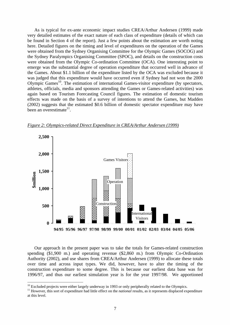
dollars in 1996 prices) as the direct expenditure on the Olympics and related activities. This formed their economic shock. While the Sydney Olympics occupied less than three weeks in the spring of 2000, the total period in which Olympics-related expenditure occurred was one of at least 7 years duration starting in 1994/95, the first full financial year following Sydney’s successful bid. CREA/Arthur Andersen assumed an Olympics period of 12 years, with the Games assuming to have an effect on tourism and debt repayment for 5 years after the event year. Figure 2 shows the time pattern of the direct Olympics-related expenditure. As can be seen in Figure 2, the Olympic expenditure shocks are classified into four main types:

• Operation of the Games;

• Construction of the Games site;

• Games-visitor expenditure; and

• Induced-tourism expenditure.

Thus induced-tourism expenditure is included as a shock because it does not arise through any model mechanism, but is supposedly generated by heightened international awareness of Australia, principally international media coverage of the Games and pre-Games stories. The estimate of this assumed expenditure was done largely on the basis of projections by the Tourism Forecasting Council (1998), but as we found in Section 2.3, ex-post analysis does not support this class of expenditure actually occurring.

9 It will be recalled from an earlier footnote that this report was written by Madden, and its results were used in Madden (2002) and Madden (2006).

7

As is typical for ex-ante economic impact studies CREA/Arthur Andersen (1999) made very detailed estimates of the exact nature of each class of expenditure (details of which can be found in Section 4 of the report). Just a few points about the estimation are worth noting here. Detailed figures on the timing and level of expenditures on the operation of the Games were obtained from the Sydney Organising Committee for the Olympic Games (SOCOG) and the Sydney Paralympics Organising Committee (SPOC), and details on the construction costs were obtained from the Olympic Co-ordination Committee (OCA). One interesting point to emerge was the substantial degree of operation expenditure that occurred well in advance of the Games. About $1.1 billion of the expenditure listed by the OCA was excluded because it was judged that this expenditure would have occurred even if Sydney had not won the 2000 Olympic Games10. The estimation of international Games-visitor expenditure (by spectators, athletes, officials, media and sponsors attending the Games or Games-related activities) was again based on Tourism Forecasting Council figures. The estimation of domestic tourism effects was made on the basis of a survey of intentions to attend the Games, but Madden (2002) suggests that the estimated $0.6 billion of domestic spectator expenditure may have been an overestimate11.

Figure 2: Olympics-related Direct Expenditure in CREA/Arthur Andersen (1999)

International Visitors

Construction

Operation

Games Visitors

0

500

1,000

1,500

2,000

2,500

94/95 95/96 96/97 97/98 98/99 99/00 00/01 01/02 02/03 03/04 04/05 05/06

$mill

ion

Our approach in the present paper was to take the totals for Games-related construction spending ($1,900 m.) and operating revenue ($2,860 m.) from Olympic Co-Ordination Authority (2002), and use shares from CREA/Arthur Andersen (1999) to allocate these totals over time and across input types. We did, however, have to alter the timing of the construction expenditure to some degree. This is because our earliest data base was for 1996/97, and thus our earliest simulation year is for the year 1997/98. We apportioned 10 Excluded projects were either largely underway in 1993 or only peripherally related to the Olympics. 11 However, this sort of expenditure had little effect on the national results, as it represents displaced expenditure at this level.

8

construction expenditure across the following years in proportion to the construction expenditure shown in Figure 2.

One advantage of using a dynamic CGE model, compared with the earlier comparative-static modelling of the Sydney Olympics, is that our shocks can be imposed in a genuine year-on-year manner. The earlier studies merely broke the shocks up into three phases and then distributed the results across each year of a phase in proportion to direct expenditure.

4. The Olympic economic impact: simulation results

4.1 Foreign tourism Foreign tourists spent $358 (excluding Games tickets) during the Olympics year. Table 1

reports national results. The simulation showed that the increase in foreign tourist spending lifted Australia’s terms of trade (row 12) by 0.09 per cent in 2000/01, allowing real consumption to be 0.02 per cent higher than basecase (row 1). The rise in the terms of trade allowed export volumes to be lower than basecase (row 5), hence the real exchange rate appreciated (row 13). As discussed in Section 2.3, our inspection of Figure 1 leads us to exclude the possibility of an induced tourism effect. Hence 2000/1 is the only year for which an increase in foreign tourist spending is modelled. As is clear from Table 1, this produces no enduring macro effects at the national level.

Table 3 reports macro results for NSW. The rise in tourism spending appears as a 0.5 per cent increase in foreign exports (row 6). Rates of return on capital in the tourism sector deviate above the baseline, leading to a small increase in investment (row 2). Labour is attracted from other states, causing a small rise in employment and real GDP in NSW (rows 9 and 10). However this causes real GDP in other states to contract (rows 2-8, Table 2).

Tables 4 and 5 report sectoral results for NSW and Australia. The sectors that gained most are those that sell tourism-related goods: Trade, Accommodation, cafes and restaurants, and Transport. Other trade-exposed sectors such as Agriculture, Mining and Manufacturing are projected to have contracted as a result of the real appreciation (row 13, table 1).

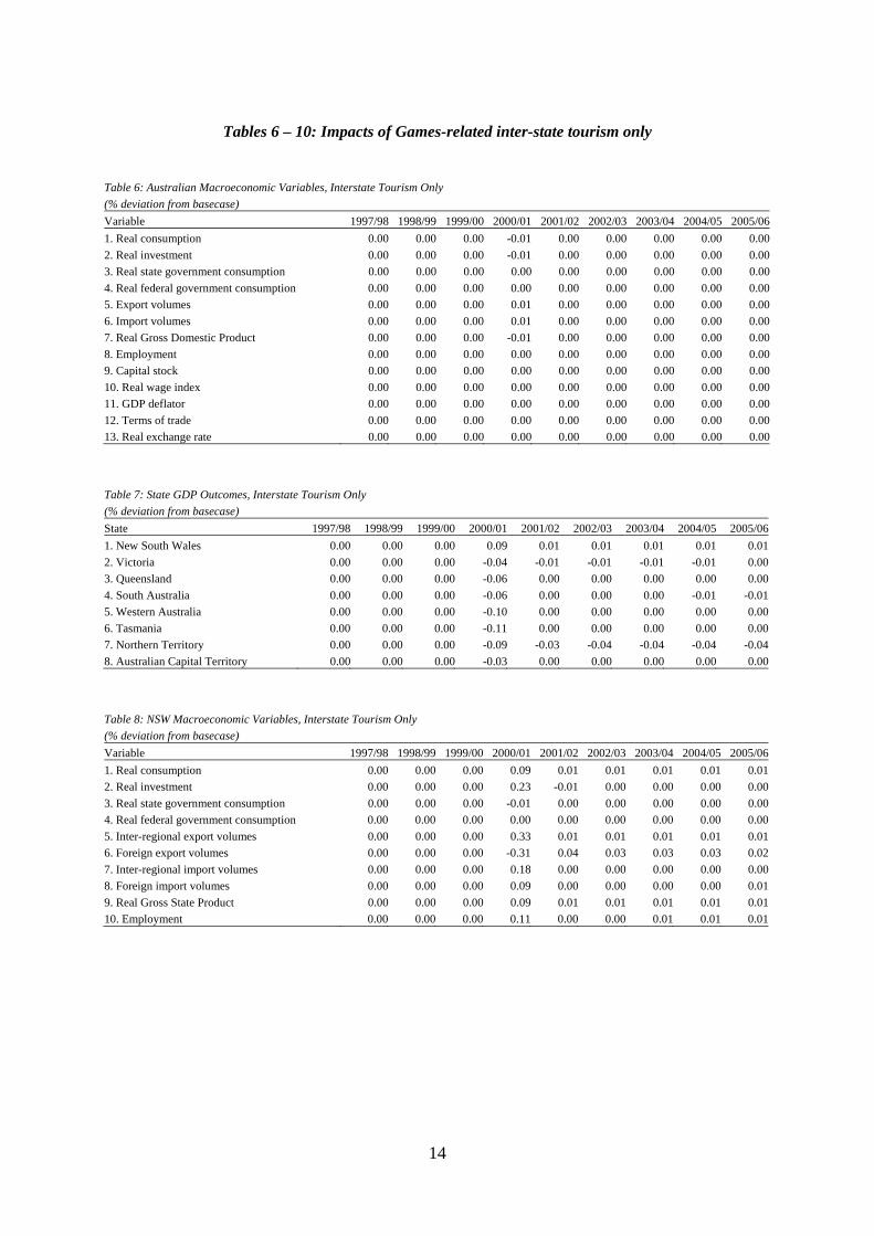
4.2 Interstate tourism Tables 6 – 10 report the effects of interstate tourism spending during the Olympics year,

independently of other Olympics-related shocks. Spending by interstate visitors to NSW during the Olympics year is modelled as a cost-neutral shift in household spending on tourism related commodities. For example, an additional $1 of spending by Victorian households on NSW tourism is matched by a $1 reduction in tourism spending by Victorians in all other Australian states. Since this just shifts final demand across Australia’s regions, there is essentially no impact on the national macro aggregates (Table 6). However the regional distribution of activity does change (Table 7). Real GDP rises in NSW (row 1, Table 7) but this is at the expense of other Australian states (rows 2-8, Table 7). Naturally, the industries that do well in NSW are those that supply goods associated with interstate tourism: Accommodation, cafes and restaurants; Transport; Cultural and recreational services; and Personal and other services (rows 7, 8, 15 and 16 of Table 10).

4.3 Construction and financing Tables 11 – 15 report the macroeconomic and sectoral effects of the Olympics

construction program. Construction spending is higher throughout 1997/98 – 2000/01. This causes real investment spending at the national and state level to be higher than basecase. At the national level, investment is approximately 0.25 per cent above basecase over the construction period (row 2, Table 1). For NSW, Olympics-related construction spending lifts aggregate NSW investment by approximately 0.75 per cent relative to basecase throughout

9

the construction phase (row 2, table 13). We assume that the NSW government finances the investment via direct taxation of NSW households. This accounts for the fall in real private consumption spending in NSW. The Olympics construction financing requirement causes NSW real private consumption spending to be approximately 0.3 per cent lower than basecase in each year leading up to and including the Olympics year.

Tables 14 and 15 report sectoral results. These reflect the shift in aggregate demand away from private consumption and towards investment. Output of the Construction sector (row 5 of Tables 14 and 15) expands as a result of Olympics-related construction activity. Sectors that sell a high proportion of their output to households (sectors 4, 7, 9, 10, 14-17) are adversely affected by Olympics financing, which requires a negative deviation in NSW consumption spending.

4.4 Olympic Operations The Olympics are initially introduced to the model as a miniature industry with a sales and

cost structure reflecting that of the actual Olympics. To get this miniature industry to its true size, we shock structural features of the model relating to demand for the sector’s output. These structural features are industry input proportions, variables relating to household tastes, and the position of the foreign demand schedule for Olympics exports.

Total Olympics sales amounted to approximately $2,860 million. Of this, approximately $730 million represented sales to firms for advertising and sponsorship rights. We model this as an intermediate input sale to Australian businesses. We assume that firms treat this as a substitute for traditional forms of marketing. As such, we simultaneously reduce demand by Australian businesses for marketing services by $730 million. Approximately $560 million of Olympics revenue comes from Australian households in the form of ticket and merchandise sales. We model this as a taste shift by Australian households towards Olympics output. This preference shift towards Olympics is matched by a shift away from consumption of other goods. Broadly, households reduce spending on other goods by $560 million, allocating this reduction across demand in proportion with household budget shares. The remaining $1,570 million of Olympics sales is to the export market (i.e. foreign purchases of tickets, the vast bulk of the TV rights, and international sponsorship). We model this as a shift in the foreign demand schedule of the Olympics industry.

The cost-side of the Olympics operations are complicated by off-SOCOG-budget items. Putting these aside for a moment, the Games use approximately $2,480 million of intermediate inputs and $370 million of labour, leaving a return to capital of $10 million. However the Games also used substantial public resources in the form of government administration, police, health and security services. These amounted to approximately $600m. While treated off-budget for accounting purposes, from an economic perspective these items should be included among the intermediate inputs used by the Olympics industry. As such, they no longer form part of public consumption spending. We model this as a reduction in public consumption spending on these services of $600m. This leaves the net output of the Public Administration sector unchanged (the sector now sells $600m. of services to the Olympics industry, but reduces its sales to public consumption by $600m). This additional $600m in intermediate inputs to the Olympics industry is paid for by the state government. We model this via a $600 million production subsidy to the industry.

Tables 16 – 20 report the macroeconomic and sectoral impacts of Olympics operations. Foreign demand for Olympics output causes a positive deviation in the terms of trade (row 12, Table 16). This accounts for the positive deviation in real national private consumption spending (row 1). However there is a negative deviation in real state government consumption (row 3). This represents the diversion of public services, such as policing, away from service

10

to households and towards input to Olympics operations. There is a small negative deviation in national real GDP (row 7), despite a small positive deviation in capital stock (row 9). This reflects the inefficiency we have built into the Olympics industry. The industry produces output worth $2.86 billion, but requires inputs of $3.46 billion. This creates an allocative efficiency loss.

NSW macro results are reported in Table 18. NSW output (row 9) expands, reflecting interstate and foreign demand for Olympics. Interstate and international sales of Olympics services are reflected in the positive deviations for NSW interstate (row 5) and international (row 6) export volumes.

Tables 19 and 20 report Australian and NSW sectoral results. The main feature of the Australian sectoral results is the fall in output of Property and business services. This reflects our assumption that businesses reduce their demand for traditional advertising services by the same amount as their sponsorship of the Olympics. In NSW, the largest expansion in industry output is experienced by Cultural and recreational services (row 15). This reflects our allocation of the Olympics industry to this sector for reporting purposes. There is no deviation in total output of Public Administration: $600 m. of government service output is diverted from public consumption to input to the Olympics industry.

5. Conclusions A summer or winter Olympic Games is a great international sporting event that brings

much enjoyment to a large number of people around the globe. For the population of the host nation increased utility arises from national-pride effects, consumer surplus on local ticket sales, the advantages of a Games being held in one's own time zone (an advantage shared by countries with a similar longitude), and so on12. As noted earlier, Atkinson (2005), found that Britons would be willing to pay £2 billion towards the cost of hosting the Games in order to obtain such intangible benefits.

The results for all of the Olympic effects in total are shown in Tables 21 to 25. This is essentially an add-up of the four groups of shocks discussed separately in Section 413. These tables clearly suggest that, in terms of purely measurable economic variables, that the Sydney Olympics had a negative effect on New South Wales and Australia as a whole. New South Wales GDP is positively affected, but not their real private and public consumption, as it is that state which covers the construction costs of the Games.

In present value terms the loss in Australian real private and public consumption shown in Table 21 is $2.1 billion. We have no estimate of willingness to pay for the Sydney Olympics by Australians. However, taking into account a possibly higher preference for sport by Australians, lower population, and making the necessary price conversion (for inflation and exchange rate), it is feasible that Australians were willing to cover this loss. However, it now seems equally unlikely that the Games produced a double dividend of intangible benefits and an economic boost of the sort previously thought. Voters were not asked if they were willing to pay (via higher taxes and/or foregone public consumption) for a loss-making Games.

As Madden (2006) warns one should be careful about translating estimates of the economic impact from one particular Olympic Games to all Games or even all mega-events. However, the results in this paper do throw the question into a different light. It is important that similar ex-post CGE modelling is performed for other Games. This should be supported by further ex-post econometric studies. Hotchkiss, et al. (2003) report econometric results 12 There might also have been some negative effects on utility such as increased congestion effects during the fortnight or so in which the Games were held. 13 It is not an exact aggregation due to the non-linearity of the MMRF model.

11

which do suggest local stimulus during the Atlanta Olympics, but there have been few such studies of Olympics (but quite a large number for other sporting operations).

Finally, as Madden (2006) argues, it is probably not possible to gauge even after the event the full extent of the labour market reaction. However, with the benefit of hindsight in the form of statistical information, our judgement is that the labour market was much tighter in the Olympics year than was formerly thought. While the question of skill shortages was raised well in advance of the Games, it was ignored in the modelling. In this paper, we make the strong assumption that there was no affect on overall Australian employment, although aggregate employment at the state level was assumed endogenous. We think there are three good reasons for doing this: (i) as Madden (2006) notes, there was a substantial elapse of time from the bid announcement to the time the bulk of the expenditure occurred, and thus anticipated labour demand increases were likely at the national level to transfer simply into a real wage rise; (ii) there are plenty of other options for fiscal stimulus if it is deemed required and thus, to consider properly the welfare effects of the Olympics, it would seem appropriate to sterilize the results from overall macroeconomic effects; and (iii) as argued above, a tight labour market would appear grounded in reality.

12

Tables 1 – 5: Impacts of Games-related foreign tourism only

Table 1: Australian Macroeconomic Variables, Foreign Tourism Only (% deviation from basecase) Variable 1997/98 1998/99 1999/00 2000/01 2001/02 2002/03 2003/04 2004/05 2005/061. Real consumption 0.00 0.00 0.00 0.02 0.00 0.00 0.00 0.00 0.002. Real investment 0.00 0.00 0.00 0.04 0.00 0.00 0.00 0.00 0.003. Real state government consumption 0.00 0.00 0.00 -0.01 0.00 0.00 0.00 0.00 0.004. Real federal government consumption 0.00 0.00 0.00 0.00 0.00 0.00 0.00 0.00 0.005. Export volumes 0.00 0.00 0.00 -0.03 0.00 0.00 0.00 0.00 0.006. Import volumes 0.00 0.00 0.00 0.07 0.00 0.00 0.00 0.00 0.007. Real Gross Domestic Product 0.00 0.00 0.00 0.00 0.00 0.00 0.00 0.00 0.008. Employment 0.00 0.00 0.00 0.00 0.00 0.00 0.00 0.00 0.009. Capital stock 0.00 0.00 0.00 0.00 0.00 0.00 0.00 0.00 0.0010. Real wage index 0.00 0.00 0.00 0.05 0.00 0.00 0.00 0.00 0.0011. GDP deflator 0.00 0.00 0.00 0.02 0.00 0.00 0.00 0.00 0.0012. Terms of trade 0.00 0.00 0.00 0.09 0.00 0.00 0.00 0.00 0.0013. Real exchange rate 0.00 0.00 0.00 0.15 0.00 0.00 0.00 0.00 0.00 Table 2: State GDP Outcomes, Foreign Tourism Only (% deviation from basecase) State 1997/98 1998/99 1999/00 2000/01 2001/02 2002/03 2003/04 2004/05 2005/061. New South Wales 0.00 0.00 0.00 0.09 0.01 0.01 0.01 0.01 0.012. Victoria 0.00 0.00 0.00 -0.05 0.00 0.00 0.00 0.00 0.003. Queensland 0.00 0.00 0.00 -0.05 0.00 0.00 0.00 0.00 0.004. South Australia 0.00 0.00 0.00 -0.06 0.00 0.00 0.00 0.00 0.005. Western Australia 0.00 0.00 0.00 -0.05 0.00 0.00 0.00 0.00 0.006. Tasmania 0.00 0.00 0.00 -0.05 0.00 0.00 0.00 0.00 0.007. Northern Territory 0.00 0.00 0.00 -0.05 0.01 0.01 0.01 0.01 0.018. Australian Capital Territory 0.00 0.00 0.00 0.00 0.00 0.00 0.00 0.00 0.00 Table 3: NSW Macroeconomic Variables, Foreign Tourism Only (% deviation from basecase) Variable 1997/98 1998/99 1999/00 2000/01 2001/02 2002/03 2003/04 2004/05 2005/061. Real consumption 0.00 0.00 0.00 0.11 0.00 0.00 0.00 0.00 0.002. Real investment 0.00 0.00 0.00 0.27 -0.01 -0.01 0.00 0.00 0.003. Real state government consumption 0.00 0.00 0.00 -0.02 0.00 0.00 0.00 0.00 0.004. Real federal government consumption 0.00 0.00 0.00 0.00 0.00 0.00 0.00 0.00 0.005. Inter-regional export volumes 0.00 0.00 0.00 -0.16 0.01 0.01 0.01 0.01 0.016. Foreign export volumes 0.00 0.00 0.00 0.52 0.04 0.03 0.03 0.02 0.027. Inter-regional import volumes 0.00 0.00 0.00 0.15 0.00 0.00 0.00 0.00 0.008. Foreign import volumes 0.00 0.00 0.00 0.16 0.00 0.00 0.00 0.00 0.009. Real Gross State Product 0.00 0.00 0.00 0.09 0.01 0.01 0.01 0.01 0.0110. Employment 0.00 0.00 0.00 0.11 0.00 0.00 0.00 0.00 0.00

13

Table 4: National Industry Outputs (% deviation from basecase), Foreign Tourism Only Australian industries 1997/98 1998/99 1999/00 2000/01 2001/02 2002/03 2003/04 2004/05 2005/061. Agriculture 0.00 0.00 0.00 -0.10 0.00 0.00 0.00 0.00 0.002. Mining 0.00 0.00 0.00 -0.06 0.00 0.00 0.00 0.00 0.003. Manufacturing 0.00 0.00 0.00 -0.12 0.00 0.00 0.00 0.00 0.004. Utilities 0.00 0.00 0.00 -0.01 0.00 0.00 0.00 0.00 0.005. Construction 0.00 0.00 0.00 0.06 0.00 0.00 0.00 0.00 0.006. Trade 0.00 0.00 0.00 -0.04 0.00 0.00 0.00 0.00 0.007. Accommodation, cafes, restaurants 0.00 0.00 0.00 0.30 0.00 0.00 0.00 0.00 0.008. Transport 0.00 0.00 0.00 0.35 0.00 -0.01 -0.01 -0.01 -0.019. Communications 0.00 0.00 0.00 0.01 0.00 0.00 0.00 0.00 0.0010. Finance 0.00 0.00 0.00 -0.02 0.00 0.00 0.00 0.00 0.0011. Property & business services 0.00 0.00 0.00 -0.02 0.00 0.00 0.00 0.00 0.0012. Public administration and defence 0.00 0.00 0.00 0.00 0.00 0.00 0.00 0.00 0.0013. Education 0.00 0.00 0.00 -0.06 0.00 0.00 0.00 0.00 0.0014. Community services 0.00 0.00 0.00 -0.01 0.00 0.00 0.00 0.00 0.0015. Cultural and recreational services 0.00 0.00 0.00 -0.01 0.00 0.00 0.00 0.00 0.0016. Personal and other services 0.00 0.00 0.00 0.02 0.00 0.00 0.00 0.00 0.0017. Ownership of dwellings 0.00 0.00 0.00 0.00 0.01 0.01 0.01 0.01 0.01 Table 5: NSW Industry Outputs (% deviation from basecase), Foreign Tourism Only Western Australian industries 1997/98 1998/99 1999/00 2000/01 2001/02 2002/03 2003/04 2004/05 2005/061. Agriculture 0.00 0.00 0.00 -0.15 0.01 0.01 0.01 0.01 0.012. Mining 0.00 0.00 0.00 -0.09 0.00 0.00 0.00 0.00 0.003. Manufacturing 0.00 0.00 0.00 -0.22 0.01 0.01 0.02 0.02 0.024. Utilities 0.00 0.00 0.00 0.03 0.00 0.00 0.00 0.00 0.005. Construction 0.00 0.00 0.00 0.22 -0.01 -0.01 -0.01 -0.01 0.006. Trade 0.00 0.00 0.00 0.04 0.01 0.01 0.01 0.01 0.017. Accommodation, cafes, restaurants 0.00 0.00 0.00 0.80 0.01 0.00 0.00 0.00 0.008. Transport 0.00 0.00 0.00 1.01 0.02 0.02 0.01 0.01 0.009. Communications 0.00 0.00 0.00 0.09 0.01 0.00 0.00 0.00 0.0010. Finance 0.00 0.00 0.00 0.02 0.01 0.01 0.00 0.00 0.0011. Property & business services 0.00 0.00 0.00 -0.01 0.00 0.00 0.00 0.00 0.0012. Public administration and defence 0.00 0.00 0.00 0.00 0.00 0.00 0.00 0.00 0.0013. Education 0.00 0.00 0.00 -0.06 0.01 0.01 0.01 0.01 0.0014. Community services 0.00 0.00 0.00 0.03 0.00 0.00 0.00 0.00 0.0015. Cultural and recreational services 0.00 0.00 0.00 0.02 0.00 0.00 0.00 0.00 0.0016. Personal and other services 0.00 0.00 0.00 0.06 0.00 0.00 0.00 0.00 0.0017. Ownership of dwellings 0.00 0.00 0.00 0.00 0.02 0.02 0.02 0.01 0.01

14

Tables 6 – 10: Impacts of Games-related inter-state tourism only

Table 6: Australian Macroeconomic Variables, Interstate Tourism Only (% deviation from basecase) Variable 1997/98 1998/99 1999/00 2000/01 2001/02 2002/03 2003/04 2004/05 2005/061. Real consumption 0.00 0.00 0.00 -0.01 0.00 0.00 0.00 0.00 0.002. Real investment 0.00 0.00 0.00 -0.01 0.00 0.00 0.00 0.00 0.003. Real state government consumption 0.00 0.00 0.00 0.00 0.00 0.00 0.00 0.00 0.004. Real federal government consumption 0.00 0.00 0.00 0.00 0.00 0.00 0.00 0.00 0.005. Export volumes 0.00 0.00 0.00 0.01 0.00 0.00 0.00 0.00 0.006. Import volumes 0.00 0.00 0.00 0.01 0.00 0.00 0.00 0.00 0.007. Real Gross Domestic Product 0.00 0.00 0.00 -0.01 0.00 0.00 0.00 0.00 0.008. Employment 0.00 0.00 0.00 0.00 0.00 0.00 0.00 0.00 0.009. Capital stock 0.00 0.00 0.00 0.00 0.00 0.00 0.00 0.00 0.0010. Real wage index 0.00 0.00 0.00 0.00 0.00 0.00 0.00 0.00 0.0011. GDP deflator 0.00 0.00 0.00 0.00 0.00 0.00 0.00 0.00 0.0012. Terms of trade 0.00 0.00 0.00 0.00 0.00 0.00 0.00 0.00 0.0013. Real exchange rate 0.00 0.00 0.00 0.00 0.00 0.00 0.00 0.00 0.00 Table 7: State GDP Outcomes, Interstate Tourism Only (% deviation from basecase) State 1997/98 1998/99 1999/00 2000/01 2001/02 2002/03 2003/04 2004/05 2005/061. New South Wales 0.00 0.00 0.00 0.09 0.01 0.01 0.01 0.01 0.012. Victoria 0.00 0.00 0.00 -0.04 -0.01 -0.01 -0.01 -0.01 0.003. Queensland 0.00 0.00 0.00 -0.06 0.00 0.00 0.00 0.00 0.004. South Australia 0.00 0.00 0.00 -0.06 0.00 0.00 0.00 -0.01 -0.015. Western Australia 0.00 0.00 0.00 -0.10 0.00 0.00 0.00 0.00 0.006. Tasmania 0.00 0.00 0.00 -0.11 0.00 0.00 0.00 0.00 0.007. Northern Territory 0.00 0.00 0.00 -0.09 -0.03 -0.04 -0.04 -0.04 -0.048. Australian Capital Territory 0.00 0.00 0.00 -0.03 0.00 0.00 0.00 0.00 0.00 Table 8: NSW Macroeconomic Variables, Interstate Tourism Only (% deviation from basecase) Variable 1997/98 1998/99 1999/00 2000/01 2001/02 2002/03 2003/04 2004/05 2005/061. Real consumption 0.00 0.00 0.00 0.09 0.01 0.01 0.01 0.01 0.012. Real investment 0.00 0.00 0.00 0.23 -0.01 0.00 0.00 0.00 0.003. Real state government consumption 0.00 0.00 0.00 -0.01 0.00 0.00 0.00 0.00 0.004. Real federal government consumption 0.00 0.00 0.00 0.00 0.00 0.00 0.00 0.00 0.005. Inter-regional export volumes 0.00 0.00 0.00 0.33 0.01 0.01 0.01 0.01 0.016. Foreign export volumes 0.00 0.00 0.00 -0.31 0.04 0.03 0.03 0.03 0.027. Inter-regional import volumes 0.00 0.00 0.00 0.18 0.00 0.00 0.00 0.00 0.008. Foreign import volumes 0.00 0.00 0.00 0.09 0.00 0.00 0.00 0.00 0.019. Real Gross State Product 0.00 0.00 0.00 0.09 0.01 0.01 0.01 0.01 0.0110. Employment 0.00 0.00 0.00 0.11 0.00 0.00 0.01 0.01 0.01

15

Table 9: National Industry Outputs (% deviation from basecase), Interstate Tourism Only Australian industries 1997/98 1998/99 1999/00 2000/01 2001/02 2002/03 2003/04 2004/05 2005/061. Agriculture 0.00 0.00 0.00 0.01 0.00 0.00 0.00 0.00 0.002. Mining 0.00 0.00 0.00 0.03 0.00 0.00 0.00 0.00 0.003. Manufacturing 0.00 0.00 0.00 -0.01 0.00 0.00 0.00 0.00 0.004. Utilities 0.00 0.00 0.00 -0.01 0.00 0.00 0.00 0.00 0.005. Construction 0.00 0.00 0.00 -0.01 -0.01 -0.01 -0.01 -0.01 -0.016. Trade 0.00 0.00 0.00 -0.01 0.00 0.00 0.00 0.00 0.007. Accommodation, cafes, restaurants 0.00 0.00 0.00 0.03 0.01 0.01 0.01 0.01 0.018. Transport 0.00 0.00 0.00 0.09 0.01 0.01 0.01 0.01 0.019. Communications 0.00 0.00 0.00 -0.01 0.00 0.00 0.00 0.00 0.0010. Finance 0.00 0.00 0.00 -0.02 0.00 0.00 0.00 0.00 0.0011. Property & business services 0.00 0.00 0.00 0.00 0.00 0.00 0.00 0.00 0.0012. Public administration and defence 0.00 0.00 0.00 0.00 0.00 0.00 0.00 0.00 0.0013. Education 0.00 0.00 0.00 -0.01 0.00 0.00 0.00 0.00 0.0014. Community services 0.00 0.00 0.00 -0.01 0.00 0.00 0.00 0.00 0.0015. Cultural and recreational services 0.00 0.00 0.00 -0.02 0.01 0.01 0.01 0.02 0.0216. Personal and other services 0.00 0.00 0.00 -0.05 0.01 0.01 0.01 0.01 0.0117. Ownership of dwellings 0.00 0.00 0.00 0.00 0.00 0.00 0.00 0.00 0.00 Table 10: NSW Industry Outputs (% deviation from basecase), Interstate Tourism Only Western Australian industries 1997/98 1998/99 1999/00 2000/01 2001/02 2002/03 2003/04 2004/05 2005/061. Agriculture 0.00 0.00 0.00 -0.07 0.01 0.01 0.00 0.00 0.002. Mining 0.00 0.00 0.00 -0.04 0.00 0.00 0.00 0.00 0.003. Manufacturing 0.00 0.00 0.00 -0.14 0.01 0.01 0.01 0.01 0.014. Utilities 0.00 0.00 0.00 0.03 0.00 0.00 0.00 0.00 0.005. Construction 0.00 0.00 0.00 0.15 -0.01 -0.01 0.00 0.00 0.006. Trade 0.00 0.00 0.00 0.06 0.01 0.01 0.01 0.01 0.017. Accommodation, cafes, restaurants 0.00 0.00 0.00 0.71 0.02 0.02 0.02 0.02 0.028. Transport 0.00 0.00 0.00 0.32 0.04 0.04 0.03 0.03 0.039. Communications 0.00 0.00 0.00 0.08 0.01 0.01 0.01 0.01 0.0010. Finance 0.00 0.00 0.00 0.03 0.01 0.00 0.00 0.00 0.0011. Property & business services 0.00 0.00 0.00 0.00 0.00 0.00 0.00 0.00 0.0012. Public administration and defence 0.00 0.00 0.00 0.00 0.00 0.00 0.00 0.00 0.0013. Education 0.00 0.00 0.00 -0.01 0.01 0.01 0.00 0.00 0.0014. Community services 0.00 0.00 0.00 0.04 0.00 0.00 0.00 0.00 0.0015. Cultural and recreational services 0.00 0.00 0.00 0.75 0.03 0.03 0.03 0.02 0.0216. Personal and other services 0.00 0.00 0.00 0.81 0.01 0.01 0.01 0.01 0.0117. Ownership of dwellings 0.00 0.00 0.00 0.00 0.02 0.02 0.02 0.02 0.01

16

Tables 11 – 15: Impacts of Games construction and construction financing only

Table 11: Australian Macroeconomic Variables, Construction and Financing Only (% deviation from basecase) Variable 1997/98 1998/99 1999/00 2000/01 2001/02 2002/03 2003/04 2004/05 2005/061. Real consumption -0.14 -0.16 -0.10 -0.05 -0.03 -0.03 -0.03 -0.02 -0.022. Real investment 0.32 0.36 0.18 0.07 0.01 0.01 0.01 0.01 0.003. Real state government consumption 0.00 0.00 0.00 0.00 0.00 0.00 0.00 0.00 0.004. Real federal government consumption 0.00 0.00 0.00 0.00 0.00 0.00 0.00 0.00 0.005. Export volumes -0.07 -0.08 -0.04 -0.02 0.00 0.00 0.00 0.00 0.006. Import volumes -0.05 -0.06 -0.03 -0.01 0.00 0.00 0.00 0.00 0.007. Real Gross Domestic Product -0.01 -0.02 -0.02 -0.02 -0.02 -0.01 -0.01 -0.01 -0.018. Employment 0.00 0.00 0.00 0.00 0.00 0.00 0.00 0.00 0.009. Capital stock 0.00 -0.02 -0.04 -0.06 -0.06 -0.06 -0.05 -0.05 -0.0410. Real wage index 0.15 0.15 0.06 0.00 -0.04 -0.04 -0.03 -0.03 -0.0311. GDP deflator 0.04 0.04 0.01 0.00 -0.01 -0.01 -0.01 -0.01 -0.0112. Terms of trade 0.02 0.02 0.01 0.00 0.00 0.00 0.00 0.00 0.0013. Real exchange rate -0.03 -0.02 -0.01 0.00 0.02 0.02 0.02 0.01 0.01 Table 12: State GDP Outcomes, Construction and Financing Only (% deviation from basecase) State 1997/98 1998/99 1999/00 2000/01 2001/02 2002/03 2003/04 2004/05 2005/061. New South Wales 0.18 0.17 0.05 -0.03 -0.08 -0.07 -0.07 -0.06 -0.062. Victoria -0.13 -0.14 -0.07 -0.02 0.02 0.02 0.02 0.02 0.023. Queensland -0.11 -0.12 -0.04 0.01 0.02 0.02 0.02 0.02 0.024. South Australia -0.11 -0.12 -0.06 -0.02 0.01 0.01 0.02 0.02 0.025. Western Australia -0.09 -0.09 -0.04 -0.01 0.02 0.02 0.02 0.02 0.026. Tasmania -0.09 -0.10 -0.04 0.01 0.02 0.02 0.02 0.02 0.027. Northern Territory -0.06 -0.06 -0.02 0.01 0.02 0.01 0.01 0.01 0.018. Australian Capital Territory -0.04 -0.05 0.01 0.05 0.00 0.00 0.00 0.00 0.00 Table 13: NSW Macroeconomic Variables, Construction and Financing Only (% deviation from basecase) Variable 1997/98 1998/99 1999/00 2000/01 2001/02 2002/03 2003/04 2004/05 2005/061. Real consumption -0.26 -0.28 -0.33 -0.37 -0.08 -0.07 -0.07 -0.07 -0.062. Real investment 1.20 1.34 0.51 -0.05 0.07 0.03 0.02 0.01 -0.013. Real state government consumption 0.00 0.00 0.00 0.00 0.00 0.00 0.00 0.00 0.004. Real federal government consumption 0.00 0.00 0.00 0.00 0.00 0.00 0.00 0.00 0.005. Inter-regional export volumes 0.05 0.02 0.15 0.25 -0.04 -0.04 -0.03 -0.03 -0.036. Foreign export volumes 0.29 0.21 0.33 0.42 -0.22 -0.20 -0.19 -0.18 -0.167. Inter-regional import volumes -0.16 -0.14 -0.23 -0.29 0.02 0.02 0.02 0.02 0.018. Foreign import volumes 0.03 0.03 -0.05 -0.10 -0.03 -0.03 -0.03 -0.03 -0.039. Real Gross State Product 0.18 0.17 0.05 -0.03 -0.08 -0.07 -0.07 -0.06 -0.0610. Employment 0.25 0.26 0.11 0.02 -0.04 -0.04 -0.04 -0.04 -0.04

17

Table 14: National Industry Outputs (% deviation from basecase), Construction and Financing Only Australian industries 1997/98 1998/99 1999/00 2000/01 2001/02 2002/03 2003/04 2004/05 2005/061. Agriculture -0.07 -0.07 -0.04 -0.02 0.00 0.00 0.00 0.00 0.002. Mining -0.05 -0.04 -0.03 -0.03 0.01 0.01 0.01 0.01 0.013. Manufacturing -0.04 -0.05 -0.02 0.00 -0.01 -0.01 0.00 0.00 0.004. Utilities -0.07 -0.08 -0.04 -0.01 0.00 0.00 0.00 0.00 0.005. Construction 0.67 0.73 0.36 0.13 0.01 0.01 0.01 0.00 0.006. Trade -0.06 -0.07 -0.04 -0.01 -0.01 -0.01 -0.01 -0.01 -0.017. Accommodation, cafes, restaurants -0.13 -0.15 -0.08 -0.07 0.02 0.02 0.02 0.02 0.028. Transport -0.06 -0.07 -0.03 -0.01 0.00 0.01 0.01 0.01 0.019. Communications -0.08 -0.09 -0.05 -0.01 -0.01 -0.01 -0.01 -0.01 -0.0110. Finance -0.09 -0.11 -0.06 -0.02 -0.03 -0.02 -0.02 -0.02 -0.0211. Property & business services -0.02 -0.02 -0.01 0.00 0.00 0.00 -0.01 -0.01 -0.0112. Public administration and defence -0.01 -0.01 0.00 0.00 0.00 0.00 0.00 0.00 0.0013. Education -0.06 -0.07 -0.03 0.00 0.00 0.00 0.00 0.00 0.0014. Community services -0.08 -0.08 -0.04 -0.01 0.00 0.00 0.00 0.00 0.0015. Cultural and recreational services -0.10 -0.12 -0.05 -0.05 0.01 0.02 0.02 0.02 0.0216. Personal and other services -0.12 -0.13 -0.06 -0.06 0.01 0.01 0.01 0.01 0.0117. Ownership of dwellings 0.00 -0.05 -0.10 -0.13 -0.14 -0.13 -0.12 -0.11 -0.10 Table 15: NSW Industry Outputs (% deviation from basecase), Construction and Financing Only Western Australian industries 1997/98 1998/99 1999/00 2000/01 2001/02 2002/03 2003/04 2004/05 2005/061. Agriculture 0.07 0.05 0.08 0.11 -0.07 -0.06 -0.06 -0.06 -0.052. Mining 0.07 0.07 0.08 0.09 -0.03 -0.03 -0.03 -0.03 -0.033. Manufacturing 0.26 0.25 0.26 0.28 -0.09 -0.10 -0.11 -0.11 -0.114. Utilities -0.07 -0.08 -0.07 -0.05 -0.01 -0.01 -0.01 -0.01 -0.015. Construction 2.15 2.33 1.04 0.21 0.12 0.09 0.08 0.07 0.066. Trade 0.06 0.05 -0.02 -0.06 -0.05 -0.04 -0.04 -0.04 -0.047. Accommodation, cafes, restaurants -0.16 -0.18 -0.17 -0.16 -0.03 -0.02 -0.02 -0.02 -0.028. Transport 0.10 0.07 0.09 0.10 -0.06 -0.06 -0.05 -0.05 -0.049. Communications -0.07 -0.09 -0.10 -0.10 -0.03 -0.02 -0.02 -0.02 -0.0210. Finance -0.09 -0.11 -0.12 -0.11 -0.05 -0.05 -0.04 -0.04 -0.0411. Property & business services -0.01 -0.01 -0.01 0.00 -0.01 -0.01 -0.01 -0.01 -0.0112. Public administration and defence 0.00 0.00 0.00 0.00 0.00 0.00 0.00 0.00 0.0013. Education -0.04 -0.06 -0.04 -0.03 -0.04 -0.04 -0.04 -0.03 -0.0314. Community services -0.13 -0.13 -0.13 -0.13 -0.01 -0.01 -0.01 -0.01 -0.0115. Cultural and recreational services -0.13 -0.14 -0.14 -0.13 -0.03 -0.02 -0.02 -0.02 -0.0216. Personal and other services -0.20 -0.20 -0.20 -0.20 -0.01 -0.01 -0.01 -0.01 -0.0117. Ownership of dwellings 0.00 -0.11 -0.22 -0.30 -0.36 -0.31 -0.28 -0.25 -0.22

18

Tables 16 – 20: Impacts of Games operations only

Table 16: Australian Macroeconomic Variables, Operations Only (% deviation from basecase) Variable 1997/98 1998/99 1999/00 2000/01 2001/02 2002/03 2003/04 2004/05 2005/061. Real consumption 0.02 0.01 0.03 0.02 0.00 0.00 0.00 0.00 0.002. Real investment 0.00 0.00 -0.01 -0.01 0.01 0.01 0.01 0.01 0.013. Real state government consumption -0.22 -0.16 -0.33 -0.28 0.00 0.00 0.00 0.00 0.004. Real federal government consumption 0.00 0.00 0.00 0.00 0.00 0.00 0.00 0.00 0.005. Export volumes 0.01 0.01 0.03 0.02 0.01 0.01 0.01 0.01 0.016. Import volumes 0.08 0.07 0.13 0.11 0.01 0.01 0.01 0.01 0.017. Real Gross Domestic Product -0.03 -0.02 -0.04 -0.04 0.00 0.00 0.00 0.00 0.008. Employment 0.00 0.00 0.00 0.00 0.00 0.00 0.00 0.00 0.009. Capital stock 0.00 0.00 0.00 0.00 0.00 0.00 0.00 0.01 0.0110. Real wage index 0.04 0.03 0.07 0.05 -0.01 -0.01 0.00 0.00 0.0011. GDP deflator 0.02 0.01 0.03 0.02 0.00 0.00 0.00 0.00 0.0012. Terms of trade 0.08 0.06 0.11 0.09 0.00 0.00 0.00 0.00 0.0013. Real exchange rate 0.12 0.08 0.16 0.12 -0.01 -0.01 -0.01 -0.01 0.00 Table 17: State GDP Outcomes, Operations Only (% deviation from basecase) State 1997/98 1998/99 1999/00 2000/01 2001/02 2002/03 2003/04 2004/05 2005/061. New South Wales 0.01 0.02 0.03 0.04 0.04 0.04 0.04 0.04 0.042. Victoria -0.05 -0.04 -0.09 -0.08 -0.02 -0.02 -0.02 -0.02 -0.023. Queensland -0.05 -0.04 -0.08 -0.08 -0.01 -0.01 -0.01 -0.01 -0.014. South Australia -0.05 -0.04 -0.09 -0.08 -0.02 -0.02 -0.02 -0.02 -0.025. Western Australia -0.05 -0.04 -0.08 -0.07 -0.01 -0.01 -0.01 -0.01 -0.016. Tasmania -0.05 -0.04 -0.07 -0.07 -0.01 -0.01 -0.01 -0.01 -0.017. Northern Territory -0.04 -0.03 -0.07 -0.08 -0.01 -0.01 -0.01 -0.01 -0.028. Australian Capital Territory 0.01 0.01 0.00 0.00 0.00 0.00 0.00 0.00 0.00 Table 18: NSW Macroeconomic Variables, Operations Only (% deviation from basecase) Variable 1997/98 1998/99 1999/00 2000/01 2001/02 2002/03 2003/04 2004/05 2005/061. Real consumption 0.10 0.08 0.16 0.14 0.02 0.02 0.02 0.02 0.022. Real investment 0.11 0.09 0.16 0.16 0.00 0.01 0.02 0.02 0.033. Real state government consumption -0.64 -0.46 -0.98 -0.83 0.00 0.00 0.00 0.00 0.004. Real federal government consumption 0.00 0.00 0.00 0.00 0.00 0.00 0.00 0.00 0.005. Inter-regional export volumes 0.07 0.06 0.13 0.10 0.02 0.02 0.02 0.02 0.026. Foreign export volumes 0.64 0.54 1.00 0.86 0.15 0.14 0.13 0.13 0.127. Inter-regional import volumes 0.35 0.26 0.51 0.45 -0.01 -0.01 -0.01 -0.01 -0.018. Foreign import volumes 0.26 0.20 0.38 0.33 0.03 0.03 0.02 0.03 0.039. Real Gross State Product 0.01 0.02 0.03 0.04 0.04 0.04 0.04 0.04 0.0410. Employment 0.11 0.09 0.17 0.15 0.02 0.02 0.02 0.02 0.02

19

Table 19: National Industry Outputs (% deviation from basecase), Operations Only Australian industries 1997/98 1998/99 1999/00 2000/01 2001/02 2002/03 2003/04 2004/05 2005/061. Agriculture -0.03 -0.02 -0.03 -0.02 0.00 0.00 0.00 0.00 0.002. Mining -0.04 -0.04 -0.07 -0.05 -0.01 -0.01 -0.01 -0.01 -0.013. Manufacturing -0.08 -0.06 -0.12 -0.10 0.00 0.01 0.01 0.01 0.014. Utilities 0.02 0.01 0.03 0.02 0.00 0.00 0.00 0.00 0.005. Construction 0.00 0.00 -0.01 -0.01 0.01 0.01 0.01 0.01 0.016. Trade 0.00 0.00 0.00 0.00 0.01 0.01 0.01 0.01 0.017. Accommodation, cafes, restaurants 0.00 0.00 0.00 -0.01 -0.04 -0.04 -0.04 -0.04 -0.048. Transport -0.04 -0.03 -0.05 -0.04 -0.01 -0.01 -0.01 -0.01 -0.019. Communications 0.09 0.07 0.13 0.12 0.01 0.01 0.01 0.01 0.0110. Finance 0.00 0.00 0.00 0.01 0.01 0.01 0.01 0.01 0.0111. Property & business services -0.04 -0.04 -0.08 -0.08 -0.02 -0.02 -0.02 -0.02 -0.0212. Public administration and defence -0.01 0.00 -0.01 -0.01 0.00 0.00 0.00 0.00 0.0013. Education -0.05 -0.04 -0.07 -0.06 0.01 0.01 0.01 0.01 0.0114. Community services -0.01 -0.01 -0.02 -0.01 0.01 0.01 0.01 0.01 0.0115. Cultural and recreational services 1.01 0.74 1.55 1.28 -0.10 -0.10 -0.10 -0.10 -0.1016. Personal and other services -0.02 -0.01 -0.03 -0.03 -0.05 -0.05 -0.05 -0.05 -0.0517. Ownership of dwellings 0.00 0.00 0.00 0.00 0.01 0.01 0.01 0.01 0.01 Table 20: NSW Industry Outputs (% deviation from basecase), Operations Only Western Australian industries 1997/98 1998/99 1999/00 2000/01 2001/02 2002/03 2003/04 2004/05 2005/061. Agriculture -0.05 -0.03 -0.06 -0.03 0.04 0.04 0.04 0.04 0.032. Mining -0.06 -0.05 -0.09 -0.06 0.01 0.01 0.01 0.01 0.013. Manufacturing -0.12 -0.08 -0.16 -0.12 0.07 0.08 0.08 0.09 0.094. Utilities 0.08 0.06 0.12 0.09 0.01 0.01 0.01 0.01 0.015. Construction 0.08 0.06 0.11 0.10 0.00 0.01 0.01 0.02 0.026. Trade 0.12 0.11 0.21 0.19 0.04 0.04 0.04 0.04 0.047. Accommodation, cafes, restaurants 0.10 0.08 0.15 0.13 0.02 0.02 0.02 0.02 0.028. Transport 0.00 0.01 0.02 0.03 0.05 0.05 0.04 0.04 0.049. Communications 0.27 0.21 0.43 0.37 0.04 0.03 0.03 0.02 0.0210. Finance 0.07 0.06 0.11 0.10 0.03 0.03 0.03 0.02 0.0211. Property & business services -0.04 -0.04 -0.10 -0.09 -0.04 -0.04 -0.04 -0.04 -0.0412. Public administration and defence 0.00 0.00 0.00 0.00 0.00 0.00 0.00 0.00 0.0013. Education -0.05 -0.03 -0.06 -0.04 0.03 0.03 0.03 0.02 0.0214. Community services 0.03 0.02 0.04 0.04 0.01 0.01 0.01 0.01 0.0115. Cultural and recreational services 2.81 2.09 4.35 3.58 -0.12 -0.13 -0.13 -0.13 -0.1316. Personal and other services 0.05 0.04 0.08 0.07 0.01 0.01 0.01 0.01 0.0117. Ownership of dwellings 0.00 0.01 0.02 0.03 0.04 0.04 0.04 0.04 0.03

20

Tables 21 – 25: Olympics, total impacts

Table 21: Australian Macroeconomic Variables, Total (% deviation from basecase) Variable 1997/98 1998/99 1999/00 2000/01 2001/02 2002/03 2003/04 2004/05 2005/061. Real consumption -0.12 -0.15 -0.07 -0.01 -0.03 -0.02 -0.02 -0.02 -0.012. Real investment 0.31 0.35 0.17 0.09 0.02 0.01 0.01 0.01 0.013. Real state government consumption -0.22 -0.16 -0.33 -0.29 0.01 0.01 0.01 0.01 0.014. Real federal government consumption 0.00 0.00 0.00 0.00 0.00 0.00 0.00 0.00 0.005. Export volumes -0.06 -0.07 -0.02 -0.01 0.01 0.01 0.01 0.01 0.016. Import volumes 0.03 0.01 0.10 0.18 0.01 0.01 0.01 0.01 0.017. Real Gross Domestic Product -0.04 -0.04 -0.06 -0.06 -0.01 -0.01 -0.01 -0.01 -0.018. Employment 0.00 0.00 0.00 0.00 0.00 0.00 0.00 0.00 0.009. Capital stock 0.00 -0.02 -0.04 -0.05 -0.06 -0.05 -0.04 -0.04 -0.0310. Real wage index 0.19 0.18 0.13 0.10 -0.04 -0.04 -0.03 -0.03 -0.0211. GDP deflator 0.06 0.05 0.04 0.04 -0.01 -0.01 -0.01 -0.01 -0.0112. Terms of trade 0.10 0.08 0.12 0.18 0.00 0.00 0.00 0.00 0.0013. Real exchange rate 0.09 0.06 0.15 0.27 0.00 0.00 0.00 0.00 0.00 Table 22: State GDP Outcomes, Total (% deviation from basecase) State 1997/98 1998/99 1999/00 2000/01 2001/02 2002/03 2003/04 2004/05 2005/061. New South Wales 0.19 0.19 0.08 0.19 -0.02 -0.02 -0.01 -0.01 -0.012. Victoria -0.18 -0.18 -0.16 -0.19 -0.01 -0.01 -0.01 0.00 0.003. Queensland -0.16 -0.16 -0.12 -0.17 0.00 0.00 0.00 0.00 0.004. South Australia -0.15 -0.16 -0.15 -0.21 -0.01 -0.01 -0.01 -0.01 -0.015. Western Australia -0.14 -0.13 -0.12 -0.23 0.00 0.00 0.00 0.01 0.016. Tasmania -0.15 -0.14 -0.11 -0.22 0.00 0.01 0.01 0.01 0.017. Northern Territory -0.10 -0.09 -0.08 -0.21 -0.01 -0.02 -0.03 -0.03 -0.038. Australian Capital Territory -0.03 -0.04 0.01 0.01 0.00 0.00 0.00 0.00 0.00 Table 23: NSW Macroeconomic Variables, Total (% deviation from basecase) Variable 1997/98 1998/99 1999/00 2000/01 2001/02 2002/03 2003/04 2004/05 2005/061. Real consumption -0.16 -0.20 -0.18 -0.02 -0.05 -0.04 -0.04 -0.03 -0.032. Real investment 1.32 1.43 0.67 0.60 0.05 0.04 0.03 0.03 0.023. Real state government consumption -0.64 -0.47 -0.98 -0.85 0.00 0.00 0.00 0.00 0.004. Real federal government consumption 0.00 0.00 0.00 0.00 0.00 0.00 0.00 0.00 0.005. Inter-regional export volumes 0.12 0.08 0.28 0.53 0.01 0.01 0.01 0.01 0.016. Foreign export volumes 0.93 0.75 1.33 1.48 0.01 0.00 0.00 0.00 0.007. Inter-regional import volumes 0.19 0.11 0.28 0.49 0.01 0.01 0.01 0.01 0.018. Foreign import volumes 0.29 0.23 0.33 0.48 0.01 0.01 0.01 0.00 0.009. Real Gross State Product 0.19 0.19 0.08 0.19 -0.02 -0.02 -0.01 -0.01 -0.0110. Employment 0.35 0.34 0.28 0.38 -0.02 -0.01 -0.01 -0.01 -0.01

21

Table 24: National Industry Outputs (% deviation from basecase), Total Australian industries 1997/98 1998/99 1999/00 2000/01 2001/02 2002/03 2003/04 2004/05 2005/061. Agriculture -0.09 -0.09 -0.07 -0.13 0.01 0.01 0.01 0.01 0.012. Mining -0.09 -0.08 -0.10 -0.11 0.00 0.00 0.00 0.00 0.003. Manufacturing -0.11 -0.10 -0.14 -0.24 0.00 0.00 0.00 0.00 0.014. Utilities -0.05 -0.06 -0.01 0.01 -0.01 -0.01 -0.01 -0.01 -0.015. Construction 0.67 0.73 0.35 0.17 0.01 0.01 0.01 0.01 0.016. Trade -0.07 -0.07 -0.04 -0.05 0.00 0.00 0.00 0.00 0.007. Accommodation, cafes, restaurants -0.13 -0.15 -0.08 0.25 -0.02 -0.02 -0.01 -0.01 -0.018. Transport -0.10 -0.10 -0.08 0.38 0.00 0.00 0.00 0.00 0.009. Communications 0.01 -0.03 0.08 0.10 0.00 0.00 0.00 0.00 0.0110. Finance -0.09 -0.11 -0.06 -0.05 -0.01 -0.01 -0.01 -0.01 0.0011. Property & business services -0.06 -0.05 -0.09 -0.09 -0.02 -0.02 -0.02 -0.02 -0.0212. Public administration and defence -0.02 -0.02 -0.01 -0.01 0.00 0.00 0.00 0.00 0.0013. Education -0.11 -0.10 -0.11 -0.13 0.01 0.01 0.01 0.01 0.0114. Community services -0.09 -0.09 -0.06 -0.04 0.00 0.00 0.00 0.00 0.0015. Cultural and recreational services 0.91 0.63 1.50 1.20 -0.08 -0.08 -0.07 -0.07 -0.0716. Personal and other services -0.14 -0.15 -0.09 -0.13 -0.03 -0.03 -0.02 -0.02 -0.0217. Ownership of dwellings 0.00 -0.05 -0.10 -0.12 -0.13 -0.11 -0.10 -0.09 -0.08 Table 25: NSW Industry Outputs (% deviation from basecase), Total Western Australian industries 1997/98 1998/99 1999/00 2000/01 2001/02 2002/03 2003/04 2004/05 2005/061. Agriculture 0.03 0.02 0.03 -0.15 -0.01 -0.01 -0.01 -0.01 -0.012. Mining 0.01 0.02 -0.01 -0.11 -0.01 -0.01 -0.01 -0.01 -0.013. Manufacturing 0.14 0.17 0.10 -0.19 0.01 0.00 0.00 0.00 0.004. Utilities 0.01 -0.02 0.05 0.11 0.00 0.00 0.00 0.00 0.005. Construction 2.23 2.40 1.15 0.68 0.10 0.09 0.09 0.08 0.076. Trade 0.18 0.16 0.19 0.23 0.01 0.01 0.01 0.01 0.017. Accommodation, cafes, restaurants -0.07 -0.10 -0.02 1.48 0.02 0.02 0.02 0.01 0.018. Transport 0.09 0.09 0.11 1.46 0.05 0.05 0.04 0.03 0.039. Communications 0.20 0.13 0.33 0.43 0.02 0.02 0.01 0.01 0.0110. Finance -0.02 -0.05 0.00 0.04 -0.01 -0.01 -0.01 -0.01 -0.0111. Property & business services -0.05 -0.05 -0.10 -0.11 -0.05 -0.05 -0.05 -0.05 -0.0512. Public administration and defence 0.00 0.00 0.00 0.00 0.00 0.00 0.00 0.00 0.0013. Education -0.09 -0.08 -0.10 -0.15 0.00 0.00 0.00 0.00 0.0014. Community services -0.10 -0.11 -0.09 -0.02 0.00 0.00 0.00 0.00 0.0015. Cultural and recreational services 2.69 1.94 4.22 4.23 -0.10 -0.11 -0.11 -0.12 -0.1216. Personal and other services -0.15 -0.16 -0.12 0.74 0.01 0.01 0.01 0.01 0.0117. Ownership of dwellings 0.00 -0.11 -0.21 -0.27 -0.27 -0.24 -0.21 -0.18 -0.16

22

References

Adams, P.D., B.R. Parmenter and J.M Horridge (2000), MMRF-GREEN: A dynamic, multi-Sectoral, multi-regional model of Australia, CoPS/IMPACT Working paper No. OP-94, October, pp. 26, available from the Centre of Policy Studies, Monash University, Melbourne.

Adams, P.D., M.J. Horridge, G. Wittwer (2003), “MMRF-GREEN: A Dynamic Multi-Regional Applied General Equilibrium Model of the Australian Economy, Based on the MMR and MONASH Models”, CoPS Working Paper G-140, Centre of Policy Studies and Impact Project, Monash University, Melbourne, pp. 70.

Atkinson, Giles; Mourato, S.; Szymanski, S. (2005) Are we willing to pay enough to 'back the bid'? Valuing the intangible impacts of hosting the Summer Olympic Games, Working Paper, Tanaka Business School, Imperial College London.

Baade, R.A. and Matheson, V.A. (2002), Bidding for the Olympics: Fool’s Gold? In C Barros, M Ibrahimo and S Szymanski (eds) Transatlantic Sport: The Comparative Economics of North American and European Sports, Edward Elgar, London.

Blake, A. (2005), The economic impact of the London 2012 Olympics, Discussion paper 2005/05, Christel DeHaan Tourism and Travel Research Institute, Nottingham University.

CREA/Arthur Andersen (1999). Economic impact study of the Sydney 2000 Olympic Games. Sydney: Arthur Andersen.

CREA/NSW Treasury (1997). The economic impact of the Sydney Olympic Games (New South Wales Treasury Research and Information Paper TRP97-10). Sydney: NSW Office of Financial Management. Retrieved October 22, 2005, from http://www.treasury.nsw.gov.au /pubs/trp97_10/index.htm

Coates, D. & Humphreys, B.R. (2003). Professional sports facilities, franchises and urban economic development. Public Finance and Management, 3(3), 335-357.

Crompton, J.L. (1995). Economic impact analysis of sports facilities and events: Eleven sources of misapplication. Journal of Sports Management, 9: 14-35.

Dixon, P.B. and M.T. Rimmer (2002), Dynamic general equilibrium modelling for forecasting and policy: a practical guide and documentation of MONASH, Contributions to Economic Analysis 256, North-Holland Publishing Company, Amsterdam, pp. xiv+338.

Giesecke, J.A. & Madden, J.R. (1996) The economic impact of hallmark events: a multiregional computable general equilibrium approach. Paper presented at the 5th World Congress of the Regional Science Association International, Rissho University, Tokyo.

Giesecke, J.A. & Madden, J.R. (2007) Regional adjustment to globalization: developing a CGE analytical framework. In RJ Cooper, KP Donaghy and GJD Hewings (eds) Globalization and Regional Economic Modeling. Springer-Verlag, Berlin.

Hotchkiss, J.L., Moore, R.E. & Zobay, S.M. (2003) Impact of the 1996 Summer Olympic Games on employment and wages in Georgia. Southern Economic Journal, 69(3), 691-704.

Kasimati, E. (2003) Economic aspects and the Summer Olympics: a review of related research. International Journal of Tourism Research, 5: 433-444.

23

KPMG (2006) Economic impact study of the Melbourne 2006 Commonwealth Games, Office of Commonwealth Games Co-ordination, Melbourne.

Madden, J.R. (2002) The economic consequences of the Sydney Olympics: The CREA/Arthur Andersen study. Current Issues in Tourism, 5(1): 7-21.

Madden, J.R. (2006) Economic and Fiscal Impacts of Mega Sporting Events: A General Equilibrium Assessment, Public Finance and Management, 6(3): 346-394, 2006.

Matheson, V.A. (2006) Mega-events: the effects of the world’s biggest sporting events on local, regional, and national economies. Working paper

Matheson, V.A. & Baade, R.A. (2004). Mega-sporting events in developing nations: Playing the way to prosperity? South African Journal of Economics, 72(5): 1084-1095.

Naqvi, F. and M. Peter (1996), A multiregional, multisectoral model of the Australian economy with an illustrative application, Australian Economic Papers, Vol. 35(66), pp. 94-113.

Olympic Co-Ordination Authority (2002) The Sydney 2000 Olympic and Paralympic Games: A report on the financial contribution by the New South Wales Government to the Sydney 2000 Games<http://www.ausport.gov.au/fulltext/2002/nsw/fin_cont_report.pdf>.

Owen, J.G. (2005) Estimating the cost and benefit of hosting Olympic Games: what can Beijing expect from its 2008 Games? Industrial Geographer, 3(1), 1-18.

Porter, P.K. (1999) Mega-sports events as municipal investments: a critique of impact analysis, in J. Fitzel, J. Gustafson and G. Hadley (eds), Sports Economics: Current Research, Praeger, Westport CT.

Rivenburgh, N., Louw, E., Loo, E. & Mersham, G. (2004) The Sydney Olympics and foreign attitudes towards Australia (Report SD0002). Gold Coast, Qld.: Sustainable Tourism Cooperative Research Centre.

Siegfried, J. & Zimbalist, A. (2000) The economics of sport teams and their communities. Journal of Economic Perspectives, 14(3):95-114.

Tourism Forecasting Council (1998) The Olympic effect: A report on the potential tourism impacts of the Sydney 2000 Games. Canberra: Commonwealth of Australia.