The Term Structure of Expected Quadratic Loss and Gain

Bruno Feunou∗ Ricardo Lopez Aliouchkin

Bank of Canada Syracuse University

Romeo Tedongap Lai Xu

ESSEC Business School Syracuse University

August 2019

Abstract

We document that the term structures of risk-neutral expected squared negative (quadraticloss) and positive (quadratic gain) returns on the S&P 500 are upward sloping on average.These shapes mainly reflect the higher premium required by investors to hedge downside risk,and the belief that potential gains will increase in the long-run. The term structures exhibitsubstantial time series variation with large negative slopes during crisis periods. Through thelens of Andersen et al. (2015)’s framework, we evaluate the ability of existing reduced-formoption pricing models to replicate these term structures. We stress that three ingredients areparticularly important: (1) the inclusion of jumps; (2) disentangling the price of negative jumprisk from its positive analog in the stochastic discount factor specification; (3) specifying threelatent factors.

Keywords: Quadratic risk premium, loss uncertainty, gain uncertainty, term structure

JEL Classification: G12

∗Corresponding Author: Bank of Canada, 234 Wellington St., Ottawa, Ontario, Canada K1A 0G9. Tel: +1 613782 8302. Email: feun@bankofcanada.ca. Feunou gratefully acknowledges financial support from the IFSID. Theviews expressed in this paper are those of the authors and do not necessarily reflect those of the Bank of Canada.

1 Introduction

The quadratic risk premium (QRP) is a measure of risk compensation used to gauge investors’

sentiments on uncertainty. The QRP is the difference between the risk-neutral and physical ex-

pected squared returns (quadratic payoff) on a stock. Yet, while the QRP can be a valuable tool

to appraise the uncertainty, it does not take into consideration the differences in various types of

uncertainty. Intuitively, investors like quadratic gains (squared positive returns)-the so-called good

uncertainty, but dislike quadratic losses (squared negative returns) -the so-called bad uncertainty.

To improve our understanding of the distribution of future stock returns and the different associated

risk compensations for the loss and gain, there is a need to further dissect the QRP.

The loss QRP, defined as the risk-neutral minus physical expectation of quadratic loss, is the

premium paid to hedge downside risk. On the other hand, the gain QRP, defined as the physical mi-

nus risk-neutral expectation of quadratic gain, is the premium received for upside risk. Essentially,

this means that a small positive QRP does not necessarily suggest that the market is less concerned

with future uncertainty. Rather, it only reflect a small asymmetry in the market’s assessment of the

gain versus loss uncertainty. In other words, in highly uncertain times with large swings in returns,

the magnitude of the loss QRP could be sizeable, yet just slightly higher than the magnitude of

its gain counterpart. Consequently, the (net) QRP, which nets up the two components will yield a

small positive value.

In this paper we investigate the term structure of the risk-neutral expected quadratic loss and

gain. We ask to what extent variations in these term structures reflect changes in the expected

path of future negative or positive squared returns and, conversely, the extent to which they reflect

changes in the risk premia. Similar questions have been investigated in the literature, but focusing

on the total variance. We extend these studies by investigating the term structure of the risk-neutral

expected quadratic loss and gain. There are two complementary explanations for an upward sloping

risk-neutral expected quadratic loss: either the market expects an increase in loss risk, or exposure

to short-term loss risk commands a lower risk premium than exposure to long-term loss risk. A

similar reasoning can be applied for an upward sloping term structure for the risk-neutral expected

quadratic gain.

Using a large panel of S&P 500 index options data with time-to-maturity ranging from 1 to

12 months, we build a model-free risk-neutral expected quadratic loss and gain term structure.

Our methodology is similar to that used to compute the VIX index. Further, using state-of-the art

1

models based on high frequency realized semi-variances, we build physical expectation counterparts.

This allows us to reveal new important findings. First, on average, the term structure of the risk-

neutral expected quadratic payoff and its loss and gain components are all upward sloping. Second,

the term structure of physical expected quadratic payoff and quadratic gain are also upward sloping,

while the physical expected quadratic loss exhibits a downward sloping term structure. This implies

that on average, investors expect total uncertainty to increase with the horizon, but also, they expect

the gain potentials to increase and the loss risk to decrease with the horizon. At the same time,

investor’s demand for insurance against negative outcomes increases with the horizon. Finally, we

find that all the term structures display important time series variations. Both the net and loss

QRP term structures invert during crises, which indicates investors’ belief in the long-term recovery.

We evaluate whether the recent state-of-the-art option pricing model of Andersen et al. (2015)

(henceforth AFT) is able to replicate the observed term structures of risk-neutral expected quadratic

payoff, its components and premia. Key features of the three-factor AFT model are its flexibility

and its ability to completely disentangle the negative from positive jump dynamics. To better

understand the statistical properties of the quadratic loss and gain, we also estimate several re-

stricted variants of the AFT model. These include, among others, the two-factor diffusion model of

Christoffersen et al. (2009) (denoted as the baseline model AFT0), and a version where the negative

jump dynamic equals its positive counterpart (denoted by AFT3). The AFT3 model essentially

represents the vast majority of option and variance swaps models studied in the literature so far

(see e.g. Bates, 2012, Christoffersen et al., 2012, Eraker, 2004, Chernov et al., 2003, Huang and

Wu, 2004, Amengual and Xiu, 2018, and Ait-Sahalia et al., 2015).1 We find that including jumps is

essential to fit the term structure of the risk-neutral expected quadratic loss and gain. The AFT0

model overestimates the risk-neutral expected quadratic gain and underestimates the risk-neutral

expected quadratic loss, but is able to fit the term structure of the risk-neutral expected quadratic

payoff. We also find that having a pure jump process is essential to fit the term structure of the

risk-neutral expected quadratic loss, while a pure diffusion process is a key ingredient for the term

structure of the risk-neutral expected quadratic gain.

In addition, we study various pricing kernel specifications required for matching the observed

dynamic term structures of the loss and gain QRP. Our general pricing kernel specification allows

for disentangling the pricing of negative and positive jumps. We estimate several restricted variants

1Some authors have considered asymmetry in the jump size distribution (see e.g. Amengual and Xiu, 2018)However, the jump size distribution is assumed to be constant and the time variation in jumps come through theintensity which is assumed to be the same regardless of the sign of the jump.

2

of the pricing kernel. Our results unequivocally point to the importance of disentangling the price

of negative jumps from the price of positive jumps. In other words, a restricted version of the

pricing kernel imposing the same price for the negative and positive jump risk (denote by RND1) is

unable to match the dynamics of the loss and gain QRP together. This restricted version represents

the vast majority of pricing kernels studied in the literature so far, and highlights its inability to

account for the joint observed dynamics of the loss and gain QRP.2

The recent growing literature on variance and variance risk premium (VRP) decomposition

into loss and gain components (referred to in the literature as bad and good, respectively) finds

that the loss VRP is almost always positive and is the main driving component of the total VRP

(see Feunou et al., 2017), while the gain VRP is positive and rather small.3 Furthermore, the loss

VRP is strongly positively related to the equity risk premium while the gain component is weakly

positively related (see Feunou et al., 2017; Kilic and Shaliastovich, 2019, and Feunou et al., 2019).

Our approach differs from this literature in two important dimensions: (1) First, our focus is on

QRP instead of VRP. We choose QRP because there is lack of consistency on how the literature

measures the VRP pertaining a premium definition. We discuss these issues and bias in depth in

Feunou et al. (2019); (2) In general, the literature focuses on a single maturity for VRP (1 month).

In this paper, we construct and study the term structure of risk-neutral expected quadratic loss

and gain, and their associated risk premiums.

Our paper is related to the recent literature that analyses the term structure of variance swaps.

Ait-Sahalia et al. (2015) and Amengual and Xiu (2018) specify reduced-form models for the term

structure of total variance. Dew-Becker et al. (2017) investigates the ability of existing structural

models in fitting the observed term structure of variance swaps. We contribute to this literature by

investigating the term structures of the two variance components. Our paper also relates to another

strand of the literature documenting the importance of analyzing loss and gain components of

variance (risk-neutral or physical) and VRP. Barndorff-Nielsen et al. (2010) provide the theoretical

arguments supporting the splitting of the total realized variance into a loss and gain components.

The remainder of the paper is organized as follows. Section 2 introduces definitions and nota-

tions of all quantities, the data, and the methodology for constructing the risk-neutral and physical

term structure of expected quadratic loss and gain, and presents key empirical facts that any eco-

2See for instance, Eraker (2004), Santa-Clara and Yan (2010), Christoffersen et al. (2012) and Bates (2012).3To the contrary of Feunou et al. (2017) and Kilic and Shaliastovich (2019) we define the gain VRP as the physical

minus the risk-neutral expectations of gain realized variance. With this definition, we interpret the gain VRP as anamount earned instead of an amount paid.

3

nomically sound model should be able to replicate. Section 3 introduces and estimates the AFT

model and provides some details on its properties, including the implied closed-form for both the

risk-neutral and physical expectation of the quadratic loss and gain. Section 4 evaluates the ability

of the AFT model and its variants in fitting the empirical facts. Section 5 concludes.

2 Methodology, Data and Preliminary Analysis

In this section we start by defining the quadratic payoff and the quadratic risk premium and its loss

and gain components. Next, we discuss the methodology to measure the term structure of the risk-

neutral and physical expectations of quadratic payoff and the term structure of the quadratic risk

premium (and its loss and gain components). For the purpose of computing these term structures,

we present the data and provide descriptive statistics. Finally, we provide a preliminary analysis

by extracting principal components of these term structures.

2.1 Definitions

Let St denote the S&P 500 index price at the end of day t and rt,t+τ denote its (log) return from

end of day t to end of day t+τ (rt,t+τ = ln (St+τ/St)). Both the log return rt,t+τ and the quadratic

payoff r2t,t+τ are subject to a gain-loss decomposition as follows:

rt,t+τ = gt,t+τ − lt,t+τ and r2t,t+τ = g2

t,t+τ + l2t,t+τ , (1)

where the gain gt,t+τ = max (rt,t+τ , 0) and the loss lt,t+τ = max (−rt,t+τ , 0), represent the positive

and negative parts of the asset payoff, respectively. In other words, the gain and the loss are

nonnegative amounts flowing in and out of an average investor’s wealth, respectively. Since the

positive gain and the positive loss cannot occur simultaneously, for any given τ, we observe that

gt,t+τ · lt,t+τ = 0. This gain loss decomposition of an asset’s payoff is exploited as an asset pricing

approach by Bernardo and Ledoit (2000).

Following Feunou et al. (2019), we define the difference between the risk-neutral and physical

expectations of quadratic payoff as QRPt and its loss and gain components QRP lt (τ) and QRP gt (τ)

as following:

QRP lt (τ) ≡ EQt

[l2t,t+τ

]− EP

t

[l2t,t+τ

]and QRP gt (τ) ≡ EP

t

[g2t,t+τ

]− EQ

t

[g2t,t+τ

], (2)

4

where P stands for the physical measure. Equation (2) shows that loss QRP (QRP l) represents

the premium paid for the insurance against fluctuations in loss uncertainty, while the gain QRP

(QRP g) is the premium earned to compensate for the fluctuations in gain uncertainty. Thus,

the (net) QRP (QRP ≡ QRP l − QRP g) represents the net cost of insuring fluctuations in loss

uncertainty, that is the premium paid for the insurance against fluctuations in loss uncertainty net

of the premium earned to compensate for the fluctuations in gain uncertainty.

2.2 Constructing Expectations

2.2.1 Inferring the Risk-neutral Expectation from Option Prices

In practice, previous literature estimates the risk-neutral conditional expectation of quadratic

payoff directly from a cross-section of option prices. Bakshi et al. (2003) provide model-free formulas

linking the risk-neutral moments of stock returns to explicit portfolios of options. These formulas

are based on the basic notion, first presented in Bakshi and Madan (2000), that any payoff over a

time horizon can be spanned by a set of options with different strikes with the same maturity as

the investment horizon.

We adopt the notation in Bakshi et al. (2003), and define Vt (τ) as the time-t price of the τ -

maturity quadratic payoff on the underlying stock. Bakshi et al. (2003) show that Vt (τ) can be

recovered from the market prices of out-of-the-money (OTM) call and put options as follows:

Vt (τ) =

∫ ∞St

1− ln (K/St)

K2/2Ct (τ ;K) dK +

∫ St

0

1 + ln (St/K)

K2/2Pt (τ ;K) dK, (3)

where St is the time-t price of underlying stock, and Ct (τ ;K) and Pt (τ ;K) are time-t option prices

with maturity τ and strike K, respectively. The risk-neutral expectation of the quadratic payoff is

then

EQt

[r2t,t+τ

]= erf τVt (τ) , (4)

where rf is the continuously compounded interest rate.

We compute Vt (τ) on each day and maturity. In theory, computing Vt (τ) requires a continuum

of strike prices, while in practice we only observe a discrete and finite set of them. Following Jiang

and Tian (2005) and others, we discretize the integrals in equation (3) by setting up a total of 1001

grid points in the moneyness (K/St) range from 1/3 to 3. First, we use cubic splines to interpolate

the implied volatility inside the available moneyness range. Second, we extrapolate the implied

5

volatility using the boundary values to fill the rest of the grid points. Third, we calculate option

prices from these 1001 implied volatilities using the Black-Scholes formula proposed by Black and

Scholes (1973).4 Next, we compute Vt (τ) if there are four or more OTM option implied volatilities

(e.g. Conrad et al., 2013 and others). Lastly, for example, to obtain Vt (30) on a given day, we

interpolate and extrapolate Vt (τ) with different τ . This process yields a daily time series of the

risk-neutral expected quadratic payoff for each maturity such as 30, 60, 90, ..., 360 days.

Note that the price of the quadratic payoff Vt (τ) in equation (3) is the sum of a portfolio of

OTM call options and a portfolio of OTM put options:

Vt (τ) = V gt (τ) + V l

t (τ) , (5)

where:

V lt (τ) =

∫ St

0

1 + ln (St/K)

K2/2Pt (τ ;K) dK and V g

t (τ) =

∫ ∞St

1− ln (K/St)

K2/2Ct (τ ;K) dK. (6)

Feunou et al. (2019) analytically prove that V lt (τ) is the price of the quadratic loss, and V g

t (τ) is

the price of the quadratic gain. Hence, the risk-neutral expectation of quadratic loss and gain are:

EQt

[l2t,t+τ

]= erf τV l

t (τ) and EQt

[g2t,t+τ

]= erf τV g

t (τ) . (7)

2.2.2 Estimating the Physical Conditional Expected Quadratic Payoff

A regression model can be used to estimate the expectations of the quadratic payoff and trun-

cated returns over different periods using actual returns data. To compute these expectations, we

assume that, conditional on time-t information, log returns rt,t+τ have a normal distribution with

mean µt,τ = Et [rt,t+τ ] = Z>t βµ and variance σ2t,τ = Et [RVt,t+τ ], where Et [RVt,t+τ ] = Z>t βσ and

RVt,t+τ is the realized variance between end of day t and end of day t+ τ . We have then:

Et[r2t,t+τ

]= µ2

t,τ + σ2t,τ and

Et[l2t,t+τ

]=

(µ2t,τ + σ2

t,τ

)Φ(−µt,τσt,τ

)− µt,τσt,τφ

(µt,τσt,τ

)Et[g2t,t+τ

]=

(µ2t,τ + σ2

t,τ

)Φ(µt,τσt,τ

)+ µt,τσt,τφ

(µt,τσt,τ

),

(8)

under the log-normality assumption, where Φ (·) and φ (·) are the standard normal cumulative

distribution functions and density, respectively. An estimate of µt,τ is obtained as the fitted value

4Since the S&P 500 options are European, we do not have issues with the early exercise premium.

6

from a linear regression of returns onto the vector of predictors, while an estimate of σ2t,τ is obtained

as the fitted value from a linear regression of the total realized variance onto the same predictors.

Those estimates are further plugged into the formulas in equation (8) to obtain estimates of the

physical expectations of the squared returns and truncated returns.

The specification of predictors in Z has been documented in a long list of previous literature. It

is now widely accepted that models based on high frequency realized variance dominates standard

GARCH-type models (e.g., Chen and Ghysels, 2011) and thus, we follow this literature. Bekaert

and Hoerova (2014) examine state-of-the-art models in the literature and consider the most general

specification, where Z is a combination of a forward-looking volatility measure, the continuous

variations, and the jump variations and negative returns in the last day, last week or last month:

RVt,t+τ = c+ αV IX2t + βmCt−21,t + βwCt−5,t + βdCt

+γmJt−21,t + γwJt−5,t + γdJt

+δmr−t−21,t + δwr−t−5,t + δdr−t + ε(τ)t+τ , (9)

where Ct and Jt are respectively the daily continuous and discontinuous component of RVt, Ct,t+l

and Jt,t+l aggregate Ct and Jt over the horizon l, r−t,t+l = min (rt,t+l, 0) where rt,t+l aggregates the

daily log-return rt. Bekaert and Hoerova (2014) focus on one month horizon τ = 21. We are also

interested in the term structure of the expected realized variance over two-month to twelve-month

horizon, τ = 21 × 2, ..., 21 × 12. To obtain a conditional term structure of the expected realized

variance, we run twelve regressions where the right hand side is identical to that of equation (9)

and the left hand side is the realized variance RVt,t+τ with different values of τ .

We also use accumulated returns rt,t+τ on the left hand side of (9) to estimate the mean value

µt,τ . Unlike the log returns and the realized variance which are both aggregatable in the time

dimension, the quadratic payoff or its loss and gain components are not. This suggests that the

term structure of physical expectations of the quadratic payoff and its components are unlikely to

be a flat line unless the mean µt,τ is negligible for all considered horizons.

7

2.3 Data

2.3.1 Option Data

For the estimation of the S&P 500 risk-neutral quadratic payoff, we rely on S&P 500 option

prices obtained from the IvyDB OptionMetrics database for the January 1996 to December 2015

period. We exclude options with missing bid-ask prices, missing implied volatility, zero bids, neg-

ative bid-ask spreads, and options with zero open interest (e.g, Carr and Wu, 2009). Following

Bakshi et al. (2003), we restrict the sample to out-of-the-money options. We further remove op-

tions with moneyness lower than 0.2 or higher than 1.8. To ensure that our results are not driven

by misleading prices, we follow Conrad et al. (2013) and exclude options that do not satisfy the

usual option price bounds e.g. call options with a price higher than the underlying, and options

with less than 7 days to maturity.

2.3.2 Return Data

To construct the physical realized variance and perform volatility forecasts, we obtain intradaily

S&P 500 cash index data spanning the period from January 1990 to December 2015 from Tick-

Data.com, for a total of 6, 542 trading days. On a given day, we use the last record in each

five-minute interval to build a grid of five-minute equity index log-returns. Following Andersen et

al. (2001, 2003) and Barndorff-Nielsen et al. (2010), we construct the realized variance on any given

trading day t, where rj,t is the jth five-minute log-return, and nt is the number of (five-minute)

intradaily returns recorded on that day.5 We add the squared overnight log-return to the realized

variance. The realized variance between day t and t + τ are computed by accumulating the daily

realized variances.

2.4 Preliminary analysis

2.4.1 The Term Structure of the Risk-Neutral Expected Quadratic Payoff

To estimate EQt

[l2t,t+τ

]or EQ

t

[g2t,t+τ

]for each maturity τ , we use options with maturity close

to τ and do interpolations.6 In Figure 1, we plot the time series average of risk-neutral expected

5On a typical trading day, we observe nt = 78 five-minute returns.6In the data, we do not always observe options with the exact maturity τ . In order to find EQ

t

[l2t,t+τ

]or EQ

t

[g2t,t+τ

]at the exact maturity τ we either interpolate or extrapolate to find the exact value. For example, if we wish to findEQt

[l2t,t+30

], i.e. with maturity τ = 30 days, we interpolate between EQ

t

[l2t,t+τ1

]and EQ

t

[l2t,t+τ2

]to obtain EQ

t

[l2t,t+30

],

where τ1 is the closest observed maturity below 30 days, and τ2 is the closest observed maturity over 30 days. Incases where we do not observe τ2 in the data, we extrapolate τ1 to obtain the exact maturity.

8

quadratic payoff and its loss and gain components for maturities of 1, 3, 6, 9 and 12 months. We find

that the average term structures of the risk-neutral expected quadratic payoff and its components

are, in general, all upward sloping.

Dew-Becker et al. (2017) compute the term structure of forward variance prices as F rv,τt ≡

EQt [RVt+τ−1,t+τ ]. The forward variance price F rv,τt is essentially the month t risk-neutral ex-

pectation of realized variance from end of month t + τ − 1 to end of month t + τ . Similarly,

we compute the term structure of forward prices for the quadratic payoff and its components as

F r,τt ≡ EQt

[r2t+τ−1,t+τ

], F l,τt ≡ EQ

t

[l2t+τ−1,t+τ

]and F g,τt ≡ EQ

t

[g2t+τ−1,t+τ

], respectively. The risk-

neutral expectations of the loss and gain components are computed following Equation (6) and

(7).

In Figure 2, we plot the term structure of average forward prices for the quadratic payoff and

its loss and gain components. These forward prices are in annualized percentage volatility units:

100 ×√

12× F τt . In Panel A, we find that the estimated term structure of forward prices for the

quadratic payoff is concave with both the level and slope similar to the forward prices in Dew-

Becker et al. (2017). Despite the differences in the sample period, our forward prices is for the

quadratic payoff while the forward prices in Dew-Becker et al. (2017) are computed from traded

variance swaps. Compared to Dew-Becker et al. (2017), we are able to separately estimate the

forward prices for the quadratic loss and gain while the loss and gain variance swaps do not exist.

In panel B and C of Figure 2, we see that the term structure of average forward prices for the

quadratic loss and gain are in general upward sloping. We also find that, across all horizons, the

quadratic loss forward prices are higher than the quadratic gain forward prices.

To investigate time variations in these term structures, Figure 3 plots the 6-month (the level) and

the 12- minus 2-month (the slope) for the risk-neutral expected quadratic payoff and its components.

We find that both the level and the slope display important time variations, and have spikes and

troughs during crises. We also notice that, although the slopes are mostly positive, they are negative

during crises. These observed patterns are in line with the fact that during crises investors expect

a recovery in the long-run rather than the short-run.

2.4.2 The Term Structure of the Physical Expected Quadratic Payoff

In Figure 4, we plot the time series average of the term structure of physical expected quadratic

payoff and its loss and gain components for maturities of 1, 3, 6, 9 and 12 months. In Panel B,

we find that the term structure of the expected quadratic loss is downward sloping. Since the

9

quadratic loss is a measure of loss uncertainty, this suggests that investors face more uncertainty

about losses in the short-run vs. the long-run. On the other hand, in Panel C, we find that the

term structure of the expected quadratic gain is upward sloping. Since the expected quadratic gain

is a measure of the gain uncertainty, this suggests that investors face more uncertainty about gains

in the long-run vs. short-run. Comparing Panel C with Panel B, we observe that the level of the

expected quadratic gain dominates the level of the expected quadratic loss across all horizons, and

even more so in the long-run, leading to the upward sloping pattern in the total expected quadratic

payoff in Panel A. The relatively larger values of the expected quadratic gain are consistent with

the fact that the S&P 500 cash index has historically yielded a positive annual return of 7%.

To evaluate the time variation in these term structures, Figure 5 plots the 6-month maturity

(the level) and the 12- minus 2-month maturity (the slope) for the expected quadratic payoff and

its components. We find substantial variations in both the level and the slope. In Panel A and C,

we find that the expected quadratic payoff and expected quadratic gain have in general positive

and occasionally negative slopes. On the other hand, the expected quadratic loss slopes in Panel

B are almost always negative and very negative during the 2008 financial crisis. These observed

patterns are in line with the fact that investors expect a growth opportunity in the long-run rather

than the short-run.

In Figure 1 and Figure 4, we observe a common upward sloping pattern for the term structures

of the risk-neutral and physical expected quadratic payoff and its components. The only exception

is the physical expected quadratic loss which is downward sloping. Bakshi et al. (2003) show that

under certain conditions, the risk-neutral distribution can be obtained by exponentially tilting the

real-world density, with the tilt determined by the risk-aversion of investors. This means that

the observed upward sloping risk-neutral expected quadratic loss vs. the downward sloping term

structure of the physical quadratic loss may be explained by investors’ increasing risk-aversion as

the investment horizon increases.

2.4.3 The Term Structure of the Quadratic Risk Premium

Next, we turn to study the term structure of the quadratic risk premium. In Figure 6, we

plot the time series average of the term structure of quadratic risk premium and its loss and gain

components for maturities of 1, 3, 6, 9 and 12 months. The loss QRP is the price investors’ pay

to hedge extreme losses during bad times. On the other hand, the gain QRP is the compensation

investors demand for weak upside potential during bad times. We find that the loss, gain and net

10

QRP are all positive across all maturities. This suggests that regardless of the investment horizon,

investors are always averse to fluctuating loss or gain uncertainty. Furthermore, we find that the

term structures of the loss and gain QRP are upward sloping. This suggests that investors are

willing to pay ( demand to earn) a higher premium to insure against strong downside risk (weak

upside potential) in the long-run. The term structure of net QRP is also upward sloping. Since

the net QRP represents the net cost of insuring fluctuations in loss uncertainty, the observed term

structure pattern suggests that this cost is increasing with the investment horizon.

In Figure 7, we plot the 6-month (the level) and the 12- minus 2-month (the slope) of the QRP

(net, loss and gain). In Panel B, the level of the loss QRP is positive in 98% of the sample. This

implies that regardless of the economic conditions, investors always seek to hedge extreme losses.

The level of loss QRP spikes in periods of high uncertainty. The slopes of the loss QRP fluctuate

and are, in general, positive (75% of the sample), but become negative, especially during crises.

This implies that during calm periods, investors are willing to pay more to hedge against downside

risk in the long-run vs. the short-run. However, during crises they are much more concerned about

hedging short-term downside risks. In Panel C, we find that the level and the slope of the gain

QRP are positive in general (85% and 88% of the sample, respectively). Hence, investors are averse

to fluctuating quadratic gain and demand a higher premium for fluctuations in gain uncertainty in

the long-run vs. short-run.

In Table 1, we present time series means and standard deviations of the risk-neutral and phys-

ical expected quadratic payoff and the quadratic risk premium together with their loss and gain

components. The mean values for the risk-neutral expected quadratic payoff increase as the matu-

rity horizon increases from 45.30 at 1 month to 49.94 at 12 months in monthly percentage squared

unites. The mean values for the physical expected quadratic payoff are much lower but also increase

as the maturity horizon increases from 26.28 at 1 month to 28.64 at 12 months. The risk-neutral

expected quadratic loss are much higher than the risk-neutral expected quadratic gain for any given

horizon and the wedge is the same for different maturity horizons. For example, at 2 months, the

risk-neutral expected quadratic loss is 33.03 and the risk-neutral expected quadratic gain is 14.84;

the wedge is about 18 which is similar to the the wedge at 4, 6, 8 and 12 months. However, the

physical expected quadratic loss are much lower than the physical expected quadratic gain for any

given horizon and this wedge is increasing as the horizon increases. For example, at 2 months,

the risk-neutral expected quadratic loss is 10.05 and the risk-neutral expected quadratic gain is

16.45; the wedge is about 6 and this wedge is strictly increasing to 16 at 12 months. Turning to

11

the quadratic risk premium and its components, on average, the quadratic risk premiums are all

positive, equal to 19.61, 20.01 and 21.32 at 1, 6, 12 months, respectively. Both the loss quadratic

risk premium and the gain quadratic risk premium are positive. However, the loss quadratic risk

premium is dominating the gain quadratic risk premium at all horizons. For example, QRP l is

21.98 while QRP g is 2.05 at 3 months; QRP l is 26.89 while QRP g is 5.78 at 9 months. These

statistics corroborate the findings on the level and the slope for all term structures previously

discussed. We also observe, for all the physical and risk-neutral expected quadratic payoffs, the

standard deviations are decreasing as the investment horizon increases. On the other hand, the

quadratic risk premium (and its components), which represent the insurance cost (either against

downside risk, upside risk or the net cost of hedging downside risk), has a similar standard deviation

in the long-run vs short-run.

2.4.4 Principal Component Analysis

In general, structural and reduced form asset pricing models have a very tight factor structure,

implying that different expectations (whether risk-neutral or physical) are all driven by a very

low number of factors (e.g., in reduced-form option pricing models the largest number of factors

considered in the literature so far is three). Nevertheless, our analysis deals with the joint term

structures of two uncertainty components (loss and gain) under two different probability measures

(Q and P). To pin down the number of factors observed in the data, we run a principal component

analysis of the term structure of four quantities: the loss and gain components of the physical

and risk-neutral expected quadratic payoff. Alternatively, one can choose to use the loss and gain

components of the physical expected quadratic payoff and the QRP or the loss and gain components

of the risk-neutral expected quadratic payoff and the QRP. There is no difference between these

three choices.

Table 2 shows the explanatory powers of the first 3 principle components. We find that the

first 3 principal components are enough to explain 91.39% of the variation of the term structure of

the loss and gain physical expected quadratic payoff and the QRP (there are 48 variables because

we include four quantities with 12 maturities). The first principal component explains 56.76%, the

second explains 26.29% and the third explains 7.98% of the variations. In Figure 8, we plot the

time series of these 3 principal components. The immediate implication of these findings is that any

model (whether reduced-form or structural) that aims to jointly fit these various terms structures

should include at least three factors.

12

3 A Model for the Joint Term Structure of Quadratic Loss and

Gain

In this section, we introduce a heuristic theoretical framework to understand the difference between

the quadratic loss and the quadratic gain. Next, we discuss the Andersen et al. (2015) model and

some variants of this three-factor model. We use the two-factor diffusion model of Christoffersen

et al. (2009) as the baseline model. Finally, we introduce a set of different specifications for the

pricing kernel, including the baseline specification in which jumps are not priced.

3.1 Dissecting the Quadratic Payoff into Loss and Gain: A Theory

For simplicity, let us denote the risk-neutral and physical expectations as the following:

µQ+n (t, τ) ≡ EQ

t

[gnt,t+τ

], µQ−n (t, τ) ≡ EQ

t

[lnt,t+τ

], and µQn (t, τ) ≡ EQ

t

[rnt,t+τ

], (10)

µP+n (t, τ) ≡ EP

t

[gnt,t+τ

], µP−n (t, τ) ≡ EP

t

[lnt,t+τ

], and µPn (t, τ) ≡ EP

t

[rnt,t+τ

], (11)

To understand the difference between µQ+2 (t, τ) and µQ−2 (t, τ), we follow Duffie et al. (2000),

µQ−2 (t, τ) =EQt

[r2t,t+τ

]+ ΛQ (t, τ)

2

µQ+2 (t, τ) =

EQt

[r2t,t+τ

]− ΛQ (t, τ)

2, (12)

where ΛQ (t, τ) , the wedge between the risk-neutral expected quadratic loss and gain, is given by:

ΛQ (t, τ) =2

π

∫ +∞

0

Im(ϕ

(2)t,τ (−iv)

)v

dv (13)

with ϕt,τ (·) being the time t conditional risk-neutral moment-generating function of rt,t+τ , and

ϕ(2)t,τ (·) its second order derivative and Im() refers to the imaginary coefficient of a complex number.

From equation (12), it is apparent that, studying the term structure of µQ−2 (t, τ) and µQ+2 (t, τ)

amounts to studying the term structure of the quadratic payoff EQt

[r2t,t+τ

]and the term structure of

ΛQ (t, τ) . Several papers in the literature have already dealt successfully with EQt

[r2t,t+τ

], and the

consensus seems to be that a two-factor diffusion model provide a good statistical representation

(see Christoffersen et al., 2009). We now try to understand conceptually the potential drivers of

the wedge ΛQ (t, τ) .

13

We use the following power series expansion of the moment generating function ϕt,τ (·):

ϕt,τ (v) =

∞∑n=0

vn

n!µQn (t, τ) ,

to establish that

ΛQ (t, τ) = limv→∞

∞∑j=1

(−1)j v2j−1

(2j − 1)(2j − 1)!µQ2j+1 (t, τ)

. (14)

which is a weighted average of odd high order non-central moments. Since only the odd high

moments are included, the wedge ΛQ (t, τ) is closely related to the asymmetry in the distribution

of rt,t+τ . In the summation, when focusing on j = 1, it is apparent that ΛQ (t, τ) is the opposite

of the third order non-central moment µQ3 (t, τ) (up to a positive multiplicative constant). Recall

that µQ3 (t, τ) is related to the first three central moments as following:

µQ3 (t, τ) = κQ3 (t, τ) + 3µQ1 (t, τ)κQ2 (t, τ) +[µQ1 (t, τ)

]3,

were κQn (t, τ) ≡ EQt

[(rt,t+τ − µQ1 (t, τ)

)n]. Hence, we conclude that the wedge between the risk-

neutral expected quadratic loss and gain increases with the asymmetry in the risk-neutral distri-

bution. A negative skewness implies larger risk-neutral expected quadratic losses, while a positive

skewness yields the opposite effect. The wedge between the risk-neutral expected quadratic loss

and gain still exist and always negative when the distribution is symmetric (all odd order central

moments for a symmetric distribution are zero). In that case, the wedge increases in absolute value

as the volatility increases.

In search of a flexible reduced form model to accommodate different kinds of distribution asym-

metry and the term structure of µQ−2 (t, τ) and µQ+2 (t, τ), we study the recent model proposed by

Andersen et al. (2015). This model is ideal for our analysis (1) it is built to disentangle the dy-

namic of the positive and negative jumps; (2) it is a three-factor framework which would maximize

the model chances of fitting the term structure of expected quadratic loss and gain and their risk

premium since we find three principal components are needed to fit the targeted term structures

in section 2.4.4; (3) Since it is an affine model, it is tractable and enables us to compute all the

quantities of interest in closed-form.

14

3.2 The Andersen et al. (2015)’s Risk-neutral Specification

In the three-factor jump-diffusive stochastic volatility model of Andersen et al. (2015), the under-

lying asset price evolves according to the following general dynamics (under Q):

dStSt−

= (rf,t − δt) dt+√V1tdW

Q1t +

√V2tdW

Q2t + η

√V3tdW

Q3t +

∫R2

(ex − 1)µQ (dt, dx, dy)

dV1t = κ1 (v1 − V1t) dt+ σ1

√V1tdB

Q1t + µ1

∫R2

x21x<0µ (dt, dx, dy)

dV2t = κ2 (v2 − V2t) dt+ σ2

√V2tdB

Q2t

dV3t = −κ3V3tdt+ µ3

∫R2

[(1− ρ3)x21x<0 + ρ3y

2]µ (dt, dx, dy) ,

where rf,t and δt refer to the instantaneous risk-free rate and the dividend yield, respectively,(WQ

1t ,WQ2t ,W

Q3t , B

Q1t, B

Q2t

)is a five-dimensional Brownian motion with corr

(WQ

1t , BQ1t

)= ρ1 and

corr(WQ

2t , BQ2t

)= ρ2, while the remaining Brownian motions are mutually independent, µQ (dt, dx, dy) ≡

µ (dt, dx, dy)− νQt (dx, dy) dt, where νQt (dx, dy) is the risk-neutral compensator for the jump mea-

sure µ, and is assumed to be

νQt (dx, dy) =(c−t 1x<0λ−e

−λ−|x| + c+t 1x>0λ+e

−λ+|x|)

1y=0

+c−t 1x=0,y<0λ−e−λ−|y|

dx⊗ dy,

(15)

where time-varying negative and positive jumps are governed by distinct coefficients: c−t and c+t ,

respectively. These coefficients evolve as affine functions of the state vectors

c−t = c−0 + c−1 V1t− + c−2 V2t− + c−3 V3t−, c+t = c+

0 + c+1 V1t− + c+

2 V2t− + c+3 V3t−.

These three factors have distinctive features: V2t is a pure diffusion process, V3t is a pure jump

process, while innovation in V1t combine a diffusion and a jump component. Furthermore, one of

the key features of the AFT model is its ability to break the tight link between expected negative

and positive jump variation imposed by other traditional jump diffusion models. More precisely,

the AFT model implies that

EQt [NJt,t+τ ] =

2

λ2−τ

EQt

[∫ t+τ

tc−s ds

], EQ

t [PJt,t+τ ] =2

λ2+τ

EQt

[∫ t+τ

tc+s ds

], (16)

15

where PJt,t+τ and NJt,t+τ are the positive and negative jump variations between t and t + τ ,

respectively.

To better understand the key features of this general model to match the observed term struc-

tures of risk-neutral expected quadratic loss and gain, we focus on two dimensions: (1) The number

of factors. Compared to the three-factor framework, we ask if two factors are enough and which

two-factor alternatives generate the best fit; (2) The model’s ability to differentiate between the

negative and positive jump distribution. We ask if the symmetric jump distribution can still fit the

term structures. We label the unrestricted general model AFT4 and consider the following nested

specifications:

• AFT0, there is no jumps. This corresponds to the two-factor diffusion model studied exten-

sively in Christoffersen et al. (2009). This is equivalent to suppressing all the jumps related

components (η = 0 and µ1 = 0) and the third factor V3t.

• AFT1, there is no pure-jump process. This corresponds to suppressing V3t.

• AFT2, there is no pure-diffusion process. This corresponds to suppressing V2t.

• AFT3, the expected negative jump variation equals the expected positive jump variation.

This corresponds to a three-factor model which assumes the same distribution for positive

and negative jumps. It is equivalent to imposing that λ− = λ+, and c−t = c+t .

The AFT3 model covers the vast majority of option and variance swaps pricing models (see e.g.

Bates, 2012, Christoffersen et al., 2012, Eraker, 2004, Chernov et al., 2003, Huang and Wu, 2004,

Amengual and Xiu, 2018, and Ait-Sahalia et al., 2015). We evaluate the impact of this assumption

not only in fitting the expected negative and positive variance, but also the observed conditional

risk-neutral skewness and kurtosis. It has been shown in previous studies (see for e.g., Feunou et

al., 2016 and Feunou et al., 2017) that the wedge between positive and negative variance is an

important driver of the conditional skewness.

3.3 The Physical Dynamic

In this paper, our goal is to understand statistical properties of stock returns distribution that

are essential to reproduce the observed term structures of µQ+2 (t, τ), µQ−2 (t, τ), µP+

2 (t, τ) and

µP−2 (t, τ), and the stochastic discount factor specifications which can replicate the observed spreads

16

µQ−2 (t, τ)− µP−2 (t, τ) and µQ+2 (t, τ)− µP+

2 (t, τ) . To do that, we next need to specify the following

physical (denote by P) dynamic for St:

dStSt−

= (rf,t − δt + erpt) dt+√V1tdW

P1t +

√V2tdW

P2t + η

√V3tdW

P3t +

∫R2

(ex − 1)µP (dt, dx, dy)

erpt = γ0 + γ1V1t + γ2V2t + γ3V3t,

where erpt refers to the instantaneous equity risk-premium, the P−dynamic of factors is:

dV1t = κP1

(vP1 − V1t

)dt+ σ1

√V1tdB

P1t + µ1

∫R2

x21x<0µ (dt, dx, dy)

dV2t = κP2

(vP2 − V2t

)dt+ σ2

√V2tdB

P2t

dV3t = −κ3V3tdt+ µ3

∫R2

[(1− ρ3)x21x<0 + ρ3y

2]µ (dt, dx, dy) ,

where(W P

1t,WP2t,W

P3t, B

P1t, B

P2t

)is a five-dimensional Brownian motion with corr

(W P

1t, BP1t

)= ρ1

and corr(W P

2t, BP2t

)= ρ2, while the remaining Brownian motions are mutually independent. Fur-

thermore, we have µP (dt, dx, dy) = µ (dt, dx, dy) − νPt (dx, dy) dt, where νPt (dx, dy) is the physical

compensator for the jump measure µ and is given by:

νPt (dx, dy) =(cP−t 1x<0λ

P−e−λP−|x| + cP+

t 1x>0λP+e−λP+|x|

)1y=0

+cP−t 1x=0,y<0λP−e−λP−|y|

dx⊗ dy,

with cP−t = cP−0 + cP−1 V1t− + cP−2 V2t− + cP−3 V3t−, cP+t = cP+

0 + cP+1 V1t− + cP+

2 V2t− + cP+3 V3t−.

The links between risk-neutral and physical shocks are dW Pjt = dWQ

jt + θrt (j) dt, for j = 1, 2, 3, and

dBPjt = dBQ

jt + θvt (j) dt, for j = 1, 2, where θvt (j) =κj(vj−Vjt)−κPj(vPj−Vjt)

σj√Vjt

, and

θrt (j) =

[(c−j

1 + λ−+

c+j

1− λ+

)−

(γj +

cP−j

1 + λP−+

cP+j

1− λP+

)]√Vjt for j = 1, 2.

θrt (3) =

[(c−3

1 + λ−+

c+3

1− λ+

)−

(γ3 +

cP−31 + λP−

+cP+

3

1− λP+

)] √V3t

η.

Given that dBQjt = ρjdW

Qjt +

√1− ρ2

jdBQjt, we have dBP

jt = ρjdWPjt +

√1− ρ2

jdBPjt, with dBP

jt =

dBQjt+θ

vt (j) dt and θvt (j) =

θvt (j)−ρjθrt (j)√1−ρ2j

. Finally, the location (γ0) in the equity risk-premium (erpt)

is γ0 =(

c−01+λ−

+c+0

1−λ+

)−(

cP−01+λP−

+cP+0

1−λP+

).

17

3.4 The Radon-Nikodym Derivative

Finally, we wrap up this section by presenting the implied Radon-Nikodym derivative (the law of

change of measure) as the product of the two derivatives separately governing the compensation of

continuous variations and jump variations:

(dQ

dP

)t

=

(dQ

dP

)ct

(dQ

dP

)jt

,

where (dQ

dP

)ct

= exp

∫ t

0θr>s dW P

s +

∫ t

0θv>s dBP

s −1

2

∫ t

0

(θr>s θrs + θv>s θvs

)ds

,

and (dQ

dP

)jt

= E(∫ t

0

∫R2

Ψs (x, y)µP (ds, dx, dy)

),

with E referring to the stochastic exponential. We also have:

Ψt (x, y) ≡ νQt (dx, dy)

νPt (dx, dy)− 1, θrs = (θrt (1) , θrt (2) , θrt (3))> , θvt =

(θvt (1) , θvt (2)

)>and

νQt (dx, dy)

νPt (dx, dy)=

c+tcP+t

λ+λP+

exp(−(λ+ − λP+

)x)

x > 0 y = 0

c−tcP−t

λ−λP−

exp((λ− − λP−

)x)

x < 0 y = 0

c−tcP−t

λ−λP−

exp((λ− − λP−

)y)

x = 0 y < 0

.

Is the premium inherent in hedging bad shocks substantially different from the one required to be

exposed to good shocks? The evidence presented in Section 2 overwhelmingly points to two very

different premia. Another more challenging question is if we need to specify a maximum flexible

pricing kernel where all the parameters for jumps intensities are shifted from Q-measure to P-

measure by different amounts, or if there is a parsimonious specification (imposes more restrictions

between the Q- and P-dynamics) that is able to simultaneously replicate the observed dynamic

of the term structures of the loss and gain QRP. To shed light on these issues, in the estimation

investigation we distinguish between the following restrictions on the Radon-Nikodym derivative

(where the unrestricted specification is labeled RND4):

1. RND0: Jumps are not priced, this is equivalent to imposing cP+j = c+

j , cP−j = c−j , for j =

0, 1, 2, 3 λP− = λ− and λP+ = λ+. Note that this is the equivalent of setting Ψt (x, y) = 0, or

equivalently(dQdP

)jt

= 1.

18

2. RND1: The price of positive jumps equals the price of negative jumps, or more formally

Ψt (x, y) is independent of the sign of x. Note that this is the implicit restriction imposed by

traditional affine jump diffusion option pricing models, e.g. Eraker (2004),Santa-Clara and

Yan (2010), Christoffersen et al. (2012) and Bates (2012).

3. RND2: Negative jumps are not priced ⇐⇒ λP− = λ−, cP−j = c−j , for j = 0, 1, 2, 3,.

4. RND3: Positive jumps are not priced ⇐⇒ λP+ = λ+, cP+j = c+

j , for j = 0, 1, 2, 3,.

4 Estimation

We largely rely on the recent paper Feunou and Okou (2018) which proposes to estimate affine

option pricing models using risk-neutral moments instead of raw option prices. Unlike option prices,

cumulants (central moments) are linear functions of unobserved factors. Hence using cumulants

enables us to circumvent major challenges usually encountered in the estimation of latent factor

option pricing models.

Given that the AFT model is affine, the linear Kalman filter appears as a natural estimation

technique. The AFT model can easily be casted in a (linear) state-space form where the measure-

ment equations relate the observed or model-free risk-neutral cumulants to the latent factors (state

variables), and the transition equations describe the dynamic of these factors. However, unlike

the setup in Feunou and Okou (2018), we are mainly interested in the term structures of expected

quadratic loss and gain which turn out to be non-linear functions of the factors. Hence we will have

two sets of measurement equations: (1) linear, which relate the risk-neutral variances and third

order cumulants to the factors; (2) non-linear, which relate the risk-neutral expected quadratic

loss and gain to the factors. We will use only the first set of measurement equations in the linear

Kalman filtering step, and conditional on the filtered factors we will compute the likelihood of the

risk-neutral expected quadratic loss and gain.

4.1 Risk-neutral Cumulants Likelihood

On a given day t, we stack together the nth-order risk-neutral cumulant observed at distinct matu-

rities in a vector denoted by CUM(n)Qt = (CUM

(n)Qt,τ1

, ..., CUM(n)Qt,τJ

)>, where n ∈ 2, 3. We further

stack the second and third cumulant vector in CUMQt =

(CUM

(2)Q>t , CUM

(3)Q>t

)>to build a

19

2J × 1 vector. This implies the following linear measurement equation:

CUMQt = Γcum0 + Γcum1 Vt + Ω1/2

cumϑcumt , (17)

where the dimension of the unobserved state vector (Vt) is 3. Notably, Γcum0 and Γcum1 are 2J × 1

and 2J × 3 matrices of coefficients whose analytical expressions depend explicitly on Q-parameters

as shown in Feunou and Okou (2018). The last term in Equation 17 is a vector of observation

errors, where Ωcum is a 2J × 2J diagonal covariance matrix, and ϑcumt denotes a 2J × 1 vector of

independent and identically distributed (i.i.d.) standard Gaussian disturbances.

As shown in Feunou and Okou (2018), the transition equations for the three factors in the AFT

model is:

Vt+1 = Φ0 + Φ1Vt + εt+1, (18)

where

Φ0 ≡ ∆tKP0 , KP

0 =

κP1 v

P1 + µ1λ

P−c

P−0

κP2 vP2

µ3λP−c

P−0

Φ1 ≡ I3 + ∆tKP1 , KP

1 =

−κP1 + µ1λ

P−c

P−1 µ1λ

P−c

P−2 µ1λ

P−c

P−3

0 −κP2 0

µ3λP−c

P−1 µ3λ

P−c

P−2 −κP3 + µ3λ

P−c

P−3

,

I3 is a 3 × 3 identity matrix, λP− = 2/(λP−)2

, and ∆t is set to 1/252 to reflect a daily time step.

Moreover, the transition noise is εt+1 ≡ (ε1t+1, ε2t+1, ε3t+1)>, with a conditional covariance matrix

V arPt (εt+1) = ∆tΣ (Vt) , where

Σ (Vt) =

σ2

1V1t + µ21λ

P∗− c

P−t 0 µ1µ3 (1− ρ3)λP∗− c

P−t

0 σ22V2t 0

µ1µ3 (1− ρ3)λP∗− cP−t 0 µ2

3

[(1− ρ3)2 + ρ2

3

]λP∗− c

P−t

,

where λP∗− = 24/(λP−)4

.

The system (17)-(18) gives the state-space representation of the AFT model. The marginal

moments (mean and variance) of the latent vector are used to initialize the filter, by setting V0|0 =

−(KP

1

)−1KP

0 , and vec(P0|0

)= ∆t (I9 − Φ1 ⊗ Φ1)−1 vec

(Σ(V0|0

)), where I9 is a 9 × 9 identity

20

matrix, and ⊗ is the Kronecker product. Now, consider that Vt|t and Pt|t are available at a generic

iteration t. Then, the filter proceeds recursively through the forecasting step:

Vt+1|t = Φ0 + Φ1Vt|t

Pt+1|t = Φ1Pt|tΦ>1 + ∆tΣ

(Vt|t)

CUMQt+1|t = Γ0 + Γ1Vt+1|t

Mt+1|t = Γ1Pt+1|tΓ>1 + Ωcum,

(19)

and the updating step:

Vt+1|t+1 =[Vt+1|t + Pt+1|tΓ

>1 M

−1t+1|t

(CUMQ

t+1 − CUMQt+1|t

)]+,

Pt+1|t+1 = Pt+1|t − Pt+1|tΓ>1 M

−1t+1|tΓ1Pt+1|t,

(20)

where [V ]+ returns a vector whose ith element is max (Vi, 0). This additional condition ensures that

latent factor estimates remain positive for all iterations — a crucial property for stochastic volatility

factors that cannot assume negative values. Finally, we construct a Gaussian quasi log-likelihood

for the cumulants:

LikCUM = −1

2

T∑t=1

[ln(

(2π)2J det(Mt|t−1

))+ ξ>t,cumM

−1t|t−1ξt,cum

], (21)

where ξt,cum ≡ CUMQt − CUM

Qt|t−1.

4.2 Risk-neutral Expected Quadratic Loss and Gain Likelihood

We use equation (12) to compute model implied µQ+2 (t, τ) and µQ−2 (t, τ) . Note that EQ

t

[r2t,t+τ

]=

CUM(2)Qt,τ +

(CUM

(1)Qt,τ

)2and both CUM

(2)Qt,τ and CUM

(1)Qt,τ are computed analytically within the

AFT framework following Feunou and Okou (2018). We follow Fang and Oosterlee (2008) and

compute ΛQ (t, τ) as:

ΛQ (t, τ) =

N−1∑k=0

Re

ϕt,τ

(ikπ

b− a

)exp

(−i kπab− a

)ωk,

21

where i stands for the imaginary unit, ω0 =

− b3−a33(b−a) if a ≥ 0

− b3+a3

3(b−a) if a < 0, and for k > 0

ωk =

−4(b−a)(b(−1)k−a)

(kπ)2if a ≥ 0

−4(b−a)(b(−1)k+a)(kπ)2

+ 8(b−a)2

(kπ)3sin(kπ a

b−a

)if a < 0

.

In the implementation phase, we set a = ln(0.01), b = −a, and N = 100. Recall that within the AFT

framework, the risk-neutral moment generation function ϕt,τ (·) is an exponential linear function of

the factor Vt.7 Hence, both µQ+

2 (t, τ) and µQ−2 (t, τ) are non-linear functions of the factor Vt:

µQ+2 (t, τ) = µQ+

2,τ (Vt) , µQ−2 (t, τ) = µQ−2,τ (Vt)

Tmom+t =

(µQ+

2,τ1, · · · , µQ+

2,τJ

)>, Tmom−t =

(µQ−2,τ1

, · · · , µQ−2,τJ

)>Tmomt =

(Tmom+>

t , Tmom−>t

)>.

We construct a Gaussian quasi log-likelihood for the truncated moments Tmomt

LikTmom = −1

2

T∑t=1

[ln(

(2π)2J det (ΩTmom))

+ ξ>t,TmomΩ−1Tmomξt,Tmom

], (22)

where ξt,Tmom = Tmom(Obs)t − Tmomt

(Vt|t), ΩTmom denotes the measurement error variance,

Tmom(Obs)t is the time t observed risk-neutral truncated moments (computed model-free using

(5)), and Vt|t is obtained through the filtering procedure (see Equation (19) and (20)). Different

models’ parameters are estimated via a maximisation of LikCUM + LikTmom.

5 Results

In this section, we evaluate the ability of different models to fit the term structure of the expected

quadratic payoff and its loss and gain components. We use Christoffersen et al. (2009) (AFT0) as

our baseline model. We compare this baseline model with two other two-factor alternatives AFT1

and AFT2 and two more three-factor models AFT3 with symmetric jump distribution and AFT4

in Andersen et al. (2015). Finally, we evaluate the ability of different pricing kernels with various

7The coefficients relating ln (ϕt,τ (·)) are a solution to Ordinary Differential Equations (ODEs) that can only besolved numerically (see the Online appendix of Andersen et al., 2015 for more details). We thank Nicola Fusari forsharing the estimation code.

22

flexibility in fitting the QRP and its loss and gain components.

5.1 Fitting the Risk-neutral Expectations

We examine the performance of different models by relying on the root-mean-squared error:

RMSE ≡

√√√√ 1

T

T∑t=1

(MomMkt

t −MomModt

)2,

where MomMktt is the time t observed risk-neutral moment and MomMod

t is the model-implied

equivalent. Results are reported in Table 3 where several conclusions can be drawn. Overall,

regarding the fitting of the term structure of the risk-neutral expected gain and loss, the benchmark

two-factors diffusion model (AFT0) is outperformed by all the other variants.

With respect to the risk neutral quadratic loss fit, the AFT0 model’s RMSE increases with

horizon and ranges from 1% at two months to 2.15% at one year. The average RMSE is 1.73%

which is far higher than other models’ RMSEs. The best performer is the AFT4 model with an

average error of 0.77% which offers approximately 56% improvement over the benchmark AFT0

model. This performance of the AFT4 model is robust across horizon, with a RMSE as low as

0.45% around horizons 4 to 5 months, which is an improvement of nearly 75% over the benchmark

AFT0 model. The three-factor models (AFT3 and AFT4) outperform the other two-factor models

(AFT1 and AFT2). The AFT4 model offers an improvement of approximately 15% over the AFT3

model, which underscores the importance of accounting for asymmetry in the jump distribution.

Turning to the risk-neutral quadratic gain fit, the AFT0 model’s average RMSE is 2.19%, which

is roughly 50% higher than other variants RMSEs. The best performing model on this front is the

AFT1 model with an average RMSE of 0.98%, while the performances of the AFT2, AFT3 and

AFT4 models are similar. However, the AFT0 model fits the term structure of the total risk-neutral

quadratic payoff remarkably well with an average RMSE of 0.44%, which confirms the findings of

Christoffersen et al. (2009). The best performer for the term structure of the total quadratic payoff

is again the AFT4 model with a RMSE of about 0.19%, which offers an improvement of about 57%

over the benchmarks AFT0 and AFT3. In accordance with our findings regarding the quadratic

loss, this result highlights the importance of asymmetry in the jump distribution for fitting the

term structure of risk-neutral variance.

On the term structure of risk-neutral skewness dimension, the benchmark AFT0 is the worst

23

performer with an average RMSE of 0.85, whereas all the other variants have similar fit, with an

average RMSE of approximately 0.15, which is almost 80% improvement over the benchmark the

benchmark AFT0. This results underscores the importance of jumps when fitting the term structure

of risk-neutral skewness. To better understand our findings, we plot in Figure 9 the observed and

models implied average term structure of risk-neutral moments. The AFT0 model is clearly unable

to fit the average term structure of risk-neutral expected quadratic gain or loss. It overestimates the

risk-neutral expected quadratic gain and underestimates the risk-neutral expected quadratic loss,

which explains why it is able to fit the term structure of the total risk-neutral expected quadratic

payoff well. Not surprisingly, the AFT0 model is outperformed by all the other variants when it

comes to fitting the term structure of skewness. The most likely explanation is that jumps are

essential to generate skewness, only accounting for the leverage effect is not enough.

The ranking between two-factor models (AFT1 and AFT2) is mixed. The model without pure

jump process (AFT1) dominates the one without pure diffusion process (AFT2) when fitting the

term structure of the risk-neutral expected quadratic loss and gain in the short end. However, this

result is reversed in the long end. Figure 9 shows that, on average, the AFT1 model fits the term

structure of the risk-neutral expected quadratic gain remarkably well, while the AFT2 model fits

the term structure of risk-neutral expected quadratic loss very well. These results suggest that

incorporating a pure jump process seems to be essential for the distribution of the loss uncertainty,

while a pure diffusion process is a key ingredient for the distribution of the gain uncertainty.

Both of the two-factor variants are outperformed by the most general specification (AFT4) which

overall is able to reproduce the term structure of the truncated and total risk-neutral moments

remarkably well. Comparing the two three-factors models (AFT3 and AFT4), we evaluate the

importance of introducing a wedge between the negative and positive jump distribution. The

results are mixed on this front. For the term structure of the risk-neutral expected quadratic loss

and the risk-neutral expected quadratic payoff, the AFT4 model clearly outperforms the AFT3

model (which has no asymmetry in the jump distribution). However, there is no clear winner for

the gain uncertainty and skewness. The AFT4 model fits better the short-end of the risk-neutral

expected quadratic gain, while the AFT3 is preferred on the long-end.

5.2 Fitting the QRPs

We focus on the most flexible specification of the AFT model (AFT4) and evaluate the fitting ability

of different pricing kernel specifications discussed in section 3.4. Figure 10 plots the observed and

24

models’ implied average term structure of the quadratic risk premium. It is readily apparent that

the most flexible Radon-Nikodym derivative (RND4) is the only one which is able to fit adequately

the average term structure of the quadratic risk premium and its loss and gain components. The

worst performer is RND0 which assumes that jumps are not priced. Not pricing jumps generates

a negative average term structure of the net and loss quadratic risk premium. Not pricing either

positive jumps (RND2) or negative jumps (RND3) is also strongly rejected. Finally, even though

a symmetric Radon-Nikodym derivative (RND1) which gives the same price to both the positive

and negative jumps, is able to replicate the positive sign for all the three term structures, it fells

short to capture the right level. Overall, it is imperative to price jumps asymmetrically in the

pricing kernel.

To confirm these visual findings, we report the root mean squared error in Table 4. The root

mean squared error (denoted by RMSE) is computed as:

RMSE ≡

√√√√ 1

T

T∑t=1

(QRPMkt

t −QRPModt

)2,

where QRPMktt is the time t observed quadratic risk premium value and QRPMod

t is the model-

implied equivalent. In addition to the Loss and Gain QRP RMSEs reported in the top panels, we

have also reported the total QRP (denote Net QRP in table, because it is the difference between

Loss and Gain QRP) in the bottom left panel and the skewness risk-premium (which is defined as

the sum of the Loss and Gain QRP) in the bottom right panel.

The numbers are roughly in line with the Figure 10’s visual findings. Except for the very short

maturity (3 month), RND4 yields the smallest RMSE across maturities and for different types of

risk premium. RND0 is the worst performer, which implies that pricing jumps is important for

the dynamic of the quadratic risk premium and its components. The average RMSE for the RND4

model is 3.5%, 1.2%, 1.4% and 3.2% for the Loss, gain, net and the sum QRP respectively. These

numbers are substantial improvements over the benchmarks RND0 (which assumes that jumps

are not priced) and RND1 (which gives the same price to both the positive and negative jumps).

To be more specific, on one hand the RND4 model offers approximately 70%, 30%, 80% and 72%

improvements over RND0 for the fitting of the Loss, gain, net and the sum QRP respectively. On

the other hand, the RND4 model offers approximately 62%, 33%, 75% and 66% improvement over

RND1 for the fitting of the Loss, gain, net and the sum QRP respectively.

25

We can further scrutinize the overall performance results by maturity. Table 4 reveals that the

superiority of the RND4 pricing kernel holds across the maturity spectrum. For the Loss, net and

sum QRP, the relative improvement increases with the maturity, and reaches 80% at the one year

horizon.

6 Conclusion

In this paper we investigate how the amount of money paid by investors to hedge negative spikes in

the stock market changes with the investment horizon. For this purpose, we estimate the quadratic

payoff and its loss and gain components across time and horizon. We uncover new empirical facts

which challenge most of the existing option and variance swaps pricing models. Among these facts,

we find an average upward sloping term structure for the risk-neutral expected quadratic payoff and

its components. We also find upward sloping term structures for the physical expected quadratic

payoff and quadratic gain but a downward sloping term structure for the physical expected quadratic

loss. There is significant time variation in the slopes of these term structures, and we observe that

they are negative and spike during financial downturns. Finally, we find that at least three principal

components are required to explain the cross-section (across maturity or horizon) of the risk-neutral

and physical expected quadratic payoff and its components.

To replicate these empirical facts we focus on the Andersen et al. (2015) model and some of its

restricted variants. This model is particularly appealing as it completely disentangles the dynamics

of negative and positive jumps. In addition, the model has three factors which is an essential

ingredient as suggested by our principal component analysis. We find that models without an

asymmetric treatment of positive and negative jumps are overall rejected as they are unable to fit

the term structure of the risk-neutral expected quadratic loss. Notably, this category of models

covers most of the existing option and variance swap pricing models found in the literature. We

also present and discuss extensively about the different pricing kernel specifications. We find that

disentangling the price of negative jumps from its positive counterpart is essential for replicating

the observed dynamic of the term structure of the loss and gain quadratic risk premium.

26

References

Ait-Sahalia, Yacine, Karaman, Mustafa, and Mancini, Loriano (2015), “The term structure ofvariance swaps and risk premia,” Working Paper, Princeton University, University of Zurichand University of Lugano .

Amengual, Dante, and Xiu, Dacheng (2018), “Resolution of policy uncertainty and sudden declinesin volatility,” Journal of Econometrics, 203(2), 297 – 315.

Andersen, Torben, Fusari, Nicola, and Todorov, Viktor (2015), “The risk premia embedded in indexoptions,” Journal of Financial Economics, 117(3), 558–584.

Andersen, Torben G., Bollerslev, Tim, Diebold, Francis X., and Ebens, Heiko (2001), “The distri-bution of realized stock return volatility,” Journal of Financial Economics, 61, 43–76.

Andersen, Torben G., Bollerslev, Tim, Diebold, Francis X., and Labys, Paul (2003), “Modeling andforecasting realized volatility,” Econometrica, 71(2), 579–625.

Bakshi, G., and Madan, D. (2000), “Spanning and Derivative-security Valuation,” Journal of Fi-nancial Economics, 55, 205–238.

Bakshi, Gurdip, Kapadia, N., and Madan, Dilip (2003), “Stock return characteristics, skew laws andthe differential pricing of individual equity options,” Review of Financial Studies, 16(1), 101–143.

Barndorff-Nielsen, Ole E., Kinnebrock, Silja, and Shephard, Neil (2010) “Measuring downside risk:realised semivariance,” in Volatility and Time Series Econometrics: Essays in Honor of RobertF. Engle, eds. T. Bollerslev, and J. Russell, and M. Watson, Oxford: Oxford University Press,pp. 117-136.

Bates, David S. (2012), “U.s. stock market crash risk, 19262010,” Journal of Financial Economics,105(2), 229 – 259.

Bekaert, Geert, and Hoerova, Marie (2014), “The vix, the variance premium and stock marketvolatility,” Journal of Econometrics, 183(2), 181 – 192. Analysis of Financial Data.

Bernardo, Antonio E., and Ledoit, Olivier (2000), “Gain, loss, and asset pricing,” Journal ofPolitical Economy, 108(1), 144–172.

Black, F., and Scholes, M. (1973), “The Pricing of Options and Corporate Liabilities,” Journal ofPolitical Economy, 81(3), 637–654.

Carr, Peter, and Wu, Liuren (2009), “Variance risk premiums,” Review Financial Studies, 22, 1311–1341.

Chen, Xilong, and Ghysels, Eric (2011), “News good or bad and its impact on volatility predictionsover multiple horizons,” The Review of Financial Studies, 24(1), 46–81.

Chernov, Mikhail, Gallant, Ronald, Ghysels, Eric, and Tauchen, George (2003), “Alternative mod-els for stock price dynamics,” Journal of Econometrics, 116, 225–257.

Christoffersen, Peter, Heston, Steven, and Jacobs, Kris (2009), “The shape and term structure ofthe index option smirk: Why multifactor stochastic volatility models work so well,” ManagementScience, 55(12), 1914–1932.

27

Christoffersen, Peter, Jacobs, Kris, and Ornthanalai, Chayawat (2012), “Dynamic jump intensitiesand risk premiums: Evidence from s&p500 returns and options,” Journal of Financial Economics,106(3), 447 – 472.

Conrad, Jennifer, Dittmar, Robert F., and Ghysels, Eric (2013), “Ex ante skewness and expectedstock returns,” The Journal of Finance, 68(1), 85–124.

Dew-Becker, Ian, Giglio, Stefano, Le, Anh, and Rodriguez, Marius (2017), “The price of variancerisk,” Journal of Financial Economics, 123(2), 225 – 250.

Duffie, Darrell, Pan, Jun, and Singleton, Kenneth (2000), “Transform analysis and option pricingfor affine jump-diffusions,” Econometrica, 68, 1343–1377.

Eraker, Bjørn (2004), “Do stock prices and volatility jump? Reconciling evidence from spot andoption prices” Journal of Finance, 59(3), 1367–1404.

Fang, Fang, and Oosterlee, Cornelis (2008), “A novel pricing method for european options basedon fourier-cosine series expansions,” SIAM J. Scientific Computing, 31, 826–848.

Feunou, Bruno, and Okou, Cedric (2018), “Risk-neutral moment-based estimation of affine optionpricing models,” Journal of Applied Econometrics, 33(7), 1007–1025.

Feunou, Bruno, Jahan-Parvar, Mohammad R., and Okou, Cedric (2017), “Downside Variance RiskPremium,” Journal of Financial Econometrics, 16(3), 341–383.

Feunou, Bruno, Jahan-Parvar, Mohammad R., and Tedongap, Romeo (2016), “Which parametricmodel for conditional skewness?” The European Journal of Finance, 22(13), 1237–1271.

Feunou, Bruno, Lopez Aliouchkin, Ricardo, Tedongap, Romeo, and Xu, Lai (2019), “Loss uncer-tainty, gain uncertainty, and expected stock returns,” Working Paper, Bank of Canada, SyracuseUniversity and ESSEC Business School.

Huang, Jing-Zhi, and Wu, Liuren (2004), “Specification analysis of option pricing models based ontime-changed levy processes,” Journal of Finance, 59(3), 1405–1439.

Jiang, G. J., and Tian, Y. S. (2005), “The Model-Free Implied Volatility and Its InformationContent,” Review of Financial Studies, 18(4), 1305–1342.

Kilic, Mete, and Shaliastovich, Ivan (2019), “Good and bad variance premia and expected returns,”Management Science, 65(6), 2522–2544.

Santa-Clara, Pedro, and Yan, Shu (2010), “Crashes, volatility, and the equity premium: Lessonsfrom s&p 500 options,” The Review of Economics and Statistics, 92(2), 435–451.

28

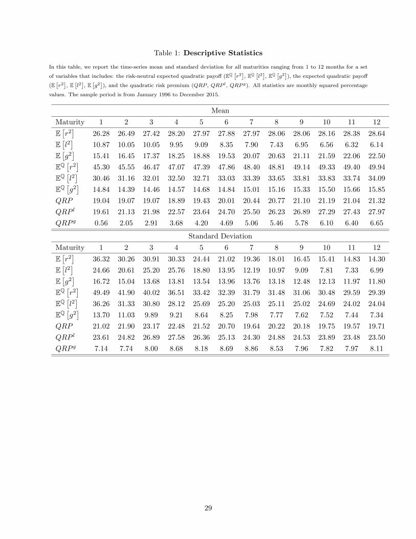
Table 1: Descriptive Statistics

In this table, we report the time-series mean and standard deviation for all maturities ranging from 1 to 12 months for a set

of variables that includes: the risk-neutral expected quadratic payoff (EQ [r2], EQ [l2], EQ [g2]), the expected quadratic payoff

(E[r2], E[l2], E[g2]), and the quadratic risk premium (QRP , QRP l, QRP g). All statistics are monthly squared percentage

values. The sample period is from January 1996 to December 2015.

Mean

Maturity 1 2 3 4 5 6 7 8 9 10 11 12

E[r2]

26.28 26.49 27.42 28.20 27.97 27.88 27.97 28.06 28.06 28.16 28.38 28.64

E[l2]

10.87 10.05 10.05 9.95 9.09 8.35 7.90 7.43 6.95 6.56 6.32 6.14

E[g2]

15.41 16.45 17.37 18.25 18.88 19.53 20.07 20.63 21.11 21.59 22.06 22.50

EQ [r2]

45.30 45.55 46.47 47.07 47.39 47.86 48.40 48.81 49.14 49.33 49.40 49.94

EQ [l2] 30.46 31.16 32.01 32.50 32.71 33.03 33.39 33.65 33.81 33.83 33.74 34.09

EQ [g2]

14.84 14.39 14.46 14.57 14.68 14.84 15.01 15.16 15.33 15.50 15.66 15.85

QRP 19.04 19.07 19.07 18.89 19.43 20.01 20.44 20.77 21.10 21.19 21.04 21.32

QRP l 19.61 21.13 21.98 22.57 23.64 24.70 25.50 26.23 26.89 27.29 27.43 27.97

QRP g 0.56 2.05 2.91 3.68 4.20 4.69 5.06 5.46 5.78 6.10 6.40 6.65

Standard Deviation

Maturity 1 2 3 4 5 6 7 8 9 10 11 12

E[r2]

36.32 30.26 30.91 30.33 24.44 21.02 19.36 18.01 16.45 15.41 14.83 14.30

E[l2]

24.66 20.61 25.20 25.76 18.80 13.95 12.19 10.97 9.09 7.81 7.33 6.99

E[g2]

16.72 15.04 13.68 13.81 13.54 13.96 13.76 13.18 12.48 12.13 11.97 11.80

EQ [r2]

49.49 41.90 40.02 36.51 33.42 32.39 31.79 31.48 31.06 30.48 29.59 29.39

EQ [l2] 36.26 31.33 30.80 28.12 25.69 25.20 25.03 25.11 25.02 24.69 24.02 24.04

EQ [g2]

13.70 11.03 9.89 9.21 8.64 8.25 7.98 7.77 7.62 7.52 7.44 7.34

QRP 21.02 21.90 23.17 22.48 21.52 20.70 19.64 20.22 20.18 19.75 19.57 19.71

QRP l 23.61 24.82 26.89 27.58 26.36 25.13 24.30 24.88 24.53 23.89 23.48 23.50

QRP g 7.14 7.74 8.00 8.68 8.18 8.69 8.86 8.53 7.96 7.82 7.97 8.11

29

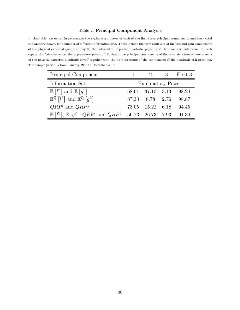
Table 2: Principal Component Analysis

In this table, we report in percentage the explanatory power of each of the first three principal components, and their total

explanatory power, for a number of different information sets. These include the term structure of the loss and gain components

of the physical expected quadratic payoff, the risk-neutral expected quadratic payoff, and the quadratic risk premium, each

separately. We also report the explanatory power of the first three principal components of the term structure of components

of the physical expected quadratic payoff together with the term structure of the components of the quadratic risk premium.

The sample period is from January 1996 to December 2015.

Principal Component 1 2 3 First 3

Information Sets Explanatory Power

E[l2]

and E[g2]

58.01 37.10 3.13 98.24

EQ [l2] and EQ [g2]

87.33 8.78 2.76 98.87

QRP l and QRP g 73.05 15.22 6.18 94.45

E[l2], E[g2], QRP l and QRP g 56.73 26.73 7.93 91.39

30

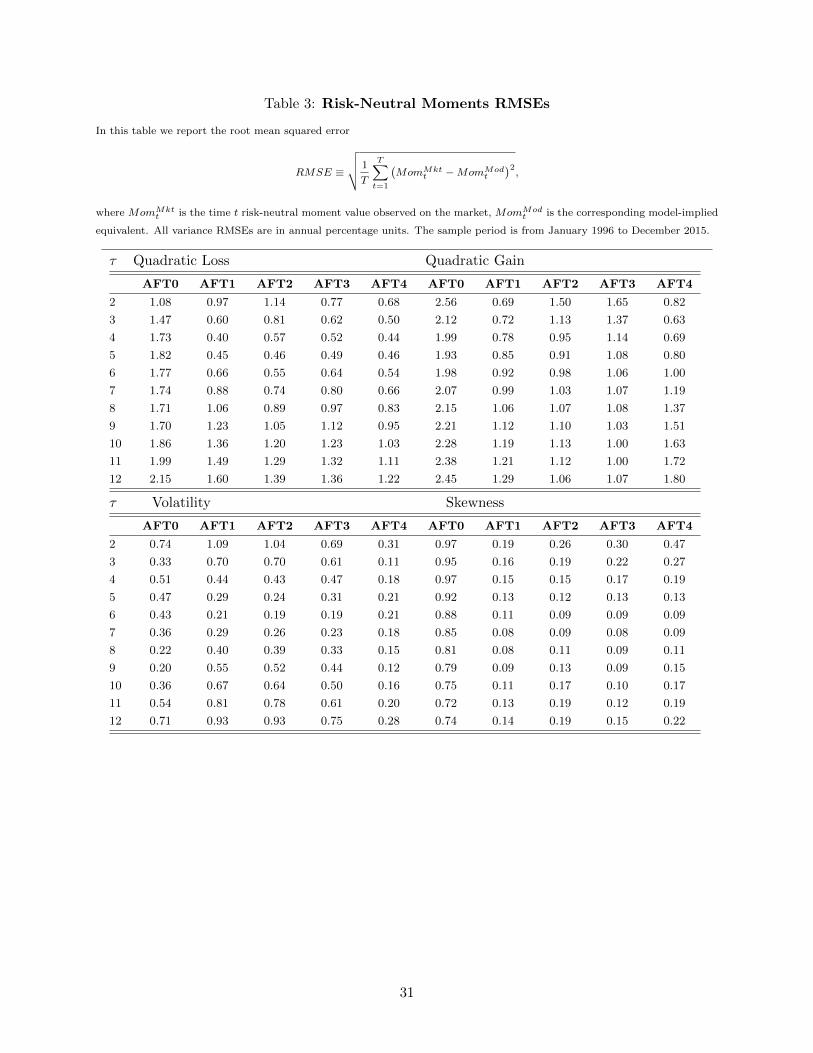
Table 3: Risk-Neutral Moments RMSEs

In this table we report the root mean squared error

RMSE ≡

√√√√ 1

T

T∑t=1

(MomMkt

t −MomModt

)2,

where MomMktt is the time t risk-neutral moment value observed on the market, MomMod

t is the corresponding model-implied

equivalent. All variance RMSEs are in annual percentage units. The sample period is from January 1996 to December 2015.

τ Quadratic Loss Quadratic Gain

AFT0 AFT1 AFT2 AFT3 AFT4 AFT0 AFT1 AFT2 AFT3 AFT4

2 1.08 0.97 1.14 0.77 0.68 2.56 0.69 1.50 1.65 0.82

3 1.47 0.60 0.81 0.62 0.50 2.12 0.72 1.13 1.37 0.63

4 1.73 0.40 0.57 0.52 0.44 1.99 0.78 0.95 1.14 0.69

5 1.82 0.45 0.46 0.49 0.46 1.93 0.85 0.91 1.08 0.80

6 1.77 0.66 0.55 0.64 0.54 1.98 0.92 0.98 1.06 1.00

7 1.74 0.88 0.74 0.80 0.66 2.07 0.99 1.03 1.07 1.19

8 1.71 1.06 0.89 0.97 0.83 2.15 1.06 1.07 1.08 1.37

9 1.70 1.23 1.05 1.12 0.95 2.21 1.12 1.10 1.03 1.51

10 1.86 1.36 1.20 1.23 1.03 2.28 1.19 1.13 1.00 1.63

11 1.99 1.49 1.29 1.32 1.11 2.38 1.21 1.12 1.00 1.72

12 2.15 1.60 1.39 1.36 1.22 2.45 1.29 1.06 1.07 1.80

τ Volatility Skewness

AFT0 AFT1 AFT2 AFT3 AFT4 AFT0 AFT1 AFT2 AFT3 AFT4

2 0.74 1.09 1.04 0.69 0.31 0.97 0.19 0.26 0.30 0.47

3 0.33 0.70 0.70 0.61 0.11 0.95 0.16 0.19 0.22 0.27

4 0.51 0.44 0.43 0.47 0.18 0.97 0.15 0.15 0.17 0.19

5 0.47 0.29 0.24 0.31 0.21 0.92 0.13 0.12 0.13 0.13

6 0.43 0.21 0.19 0.19 0.21 0.88 0.11 0.09 0.09 0.09

7 0.36 0.29 0.26 0.23 0.18 0.85 0.08 0.09 0.08 0.09

8 0.22 0.40 0.39 0.33 0.15 0.81 0.08 0.11 0.09 0.11

9 0.20 0.55 0.52 0.44 0.12 0.79 0.09 0.13 0.09 0.15

10 0.36 0.67 0.64 0.50 0.16 0.75 0.11 0.17 0.10 0.17

11 0.54 0.81 0.78 0.61 0.20 0.72 0.13 0.19 0.12 0.19

12 0.71 0.93 0.93 0.75 0.28 0.74 0.14 0.19 0.15 0.22

31

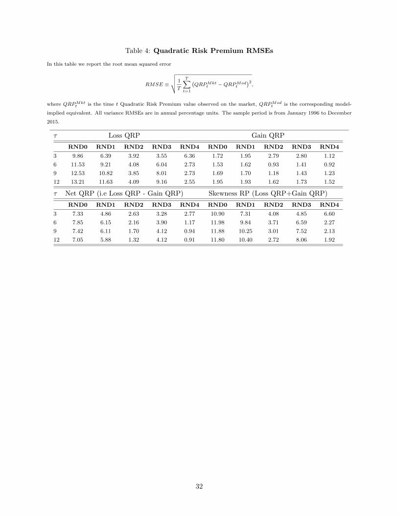
Table 4: Quadratic Risk Premium RMSEs

In this table we report the root mean squared error

RMSE ≡

√√√√ 1

T

T∑t=1

(QRPMkt

t −QRPModt

)2,

where QRPMktt is the time t Quadratic Risk Premium value observed on the market, QRPMod

t is the corresponding model-

implied equivalent. All variance RMSEs are in annual percentage units. The sample period is from January 1996 to December

2015.

τ Loss QRP Gain QRP

RND0 RND1 RND2 RND3 RND4 RND0 RND1 RND2 RND3 RND4

3 9.86 6.39 3.92 3.55 6.36 1.72 1.95 2.79 2.80 1.12

6 11.53 9.21 4.08 6.04 2.73 1.53 1.62 0.93 1.41 0.92

9 12.53 10.82 3.85 8.01 2.73 1.69 1.70 1.18 1.43 1.23

12 13.21 11.63 4.09 9.16 2.55 1.95 1.93 1.62 1.73 1.52

τ Net QRP (i.e Loss QRP - Gain QRP) Skewness RP (Loss QRP+Gain QRP)

RND0 RND1 RND2 RND3 RND4 RND0 RND1 RND2 RND3 RND4

3 7.33 4.86 2.63 3.28 2.77 10.90 7.31 4.08 4.85 6.60

6 7.85 6.15 2.16 3.90 1.17 11.98 9.84 3.71 6.59 2.27

9 7.42 6.11 1.70 4.12 0.94 11.88 10.25 3.01 7.52 2.13

12 7.05 5.88 1.32 4.12 0.91 11.80 10.40 2.72 8.06 1.92

32

Figure 1: Term Structure of Risk-Neutral Expected Quadratic Payoff

In this figure we plot the mean S&P 500 risk-neutral expected quadratic payoff in Panel A, and its loss and gain components,

in Panel B and C respectively, for maturities of 1, 3, 6, 9 and 12 months. The sample period is from January 1996 to December

2015.

1 2 3 4 5 6 7 8 9 10 11 1245

46

47

48

49

50

51

Tot

al Q

P

Panel A: Risk-Neutral Expected Quadratic Payoff

1 2 3 4 5 6 7 8 9 10 11 1230

31

32

33

34

35

Loss

QP

Panel B: Risk-Neutral Expected Loss Quadratic Payoff

1 2 3 4 5 6 7 8 9 10 11 12

Maturity (months)

14

14.5

15

15.5

16

Gai

n Q

P

Panel C: Risk-Neutral Expected Gain Quadratic Payoff

33

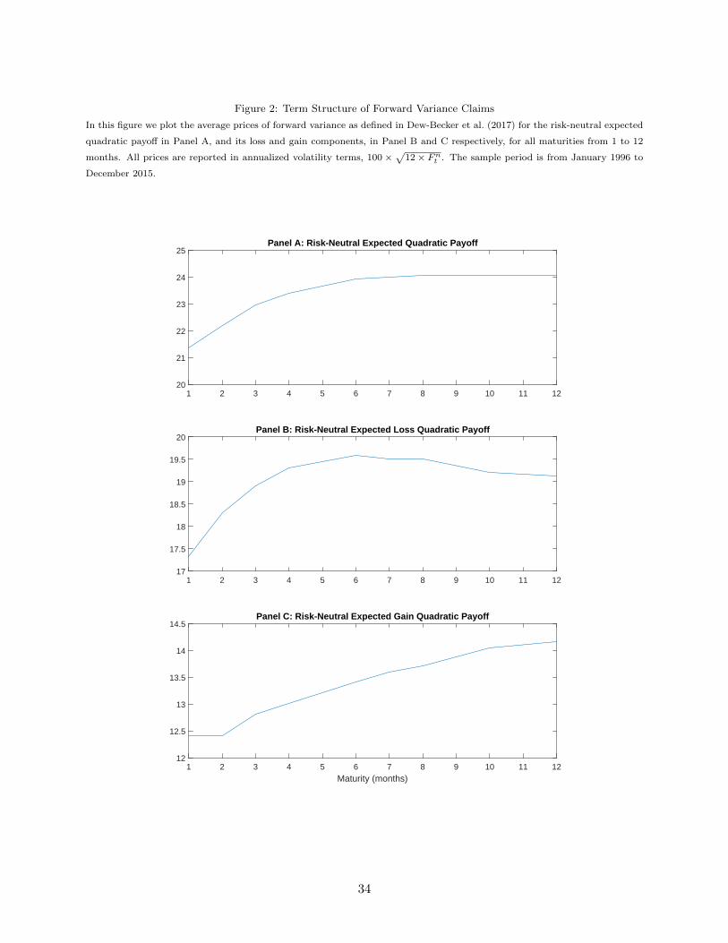
Figure 2: Term Structure of Forward Variance Claims

In this figure we plot the average prices of forward variance as defined in Dew-Becker et al. (2017) for the risk-neutral expected

quadratic payoff in Panel A, and its loss and gain components, in Panel B and C respectively, for all maturities from 1 to 12

months. All prices are reported in annualized volatility terms, 100 ×√

12× Fnt . The sample period is from January 1996 to

December 2015.

1 2 3 4 5 6 7 8 9 10 11 1220

21

22

23

24

25Panel A: Risk-Neutral Expected Quadratic Payoff

1 2 3 4 5 6 7 8 9 10 11 1217

17.5

18

18.5

19

19.5

20Panel B: Risk-Neutral Expected Loss Quadratic Payoff

1 2 3 4 5 6 7 8 9 10 11 12

Maturity (months)

12

12.5

13

13.5

14

14.5Panel C: Risk-Neutral Expected Gain Quadratic Payoff

34

Figure 3: Risk-neutral Expected Quadratic Payoff Different Maturities

In this figure we plot the 6-month and the 12- minus 2-month maturity S&P500 risk-neutral expected quadratic payoff in Panel

A, and its loss and gain components in Panel B and C, respectively. The sample period is from January 1996 to December

2015.

1996 1998 2000 2002 2004 2006 2008 2010 2012 2014 2016

-200

-100

0

100

200

300

Tot

al Q

P

Panel A: Risk-Neutral Expected Quadratic Payoff

6-month maturity12 minus 2 month maturity

1996 1998 2000 2002 2004 2006 2008 2010 2012 2014 2016

-100

0

100

200

Loss

QP

Panel B: Risk-Neutral Expected Loss Quadratic Payoff

6-month maturity12 minus 2 month maturity

1996 1998 2000 2002 2004 2006 2008 2010 2012 2014 2016

Date

-60

-40

-20

0

20

40

60

80

Gai

n Q

P

Panel C: Risk-Neutral Expected Gain Quadratic Payoff

6-month maturity12 minus 2 month maturity

35

Figure 4: Term Structure of Physical Expected Quadratic Payoff

In this figure we plot the mean S&P 500 physical expected quadratic payoff in Panel A, and its loss and gain components, in

Panel B and C respectively, for maturities of 1, 3, 6, 9 and 12 months. The sample period is from January 1996 to December

2015.

1 2 3 4 5 6 7 8 9 10 11 1225

26

27

28

29

30

Tot

al Q

P

Panel A: Physical Expected Quadratic Payoff

1 2 3 4 5 6 7 8 9 10 11 125

7

9

11

13

15

Loss

QP

Panel B: Physical Expected Loss Quadratic Payoff

1 2 3 4 5 6 7 8 9 10 11 12

Maturity (months)

15

17

19

21

23

25

Gai

n Q

P

Panel C: Physical Expected Gain Quadratic Payoff

36

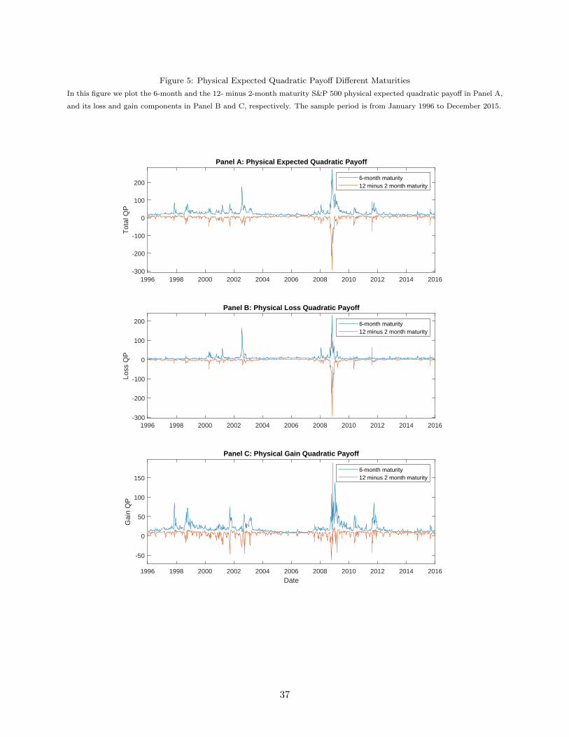
Figure 5: Physical Expected Quadratic Payoff Different Maturities

In this figure we plot the 6-month and the 12- minus 2-month maturity S&P 500 physical expected quadratic payoff in Panel A,

and its loss and gain components in Panel B and C, respectively. The sample period is from January 1996 to December 2015.

1996 1998 2000 2002 2004 2006 2008 2010 2012 2014 2016-300

-200

-100

0

100

200

Tot

al Q

P

Panel A: Physical Expected Quadratic Payoff

6-month maturity12 minus 2 month maturity

1996 1998 2000 2002 2004 2006 2008 2010 2012 2014 2016-300

-200

-100

0

100

200

Loss

QP

Panel B: Physical Loss Quadratic Payoff

6-month maturity12 minus 2 month maturity

1996 1998 2000 2002 2004 2006 2008 2010 2012 2014 2016

Date

-50

0

50

100

150

Gai

n Q

P

Panel C: Physical Gain Quadratic Payoff

6-month maturity12 minus 2 month maturity

37

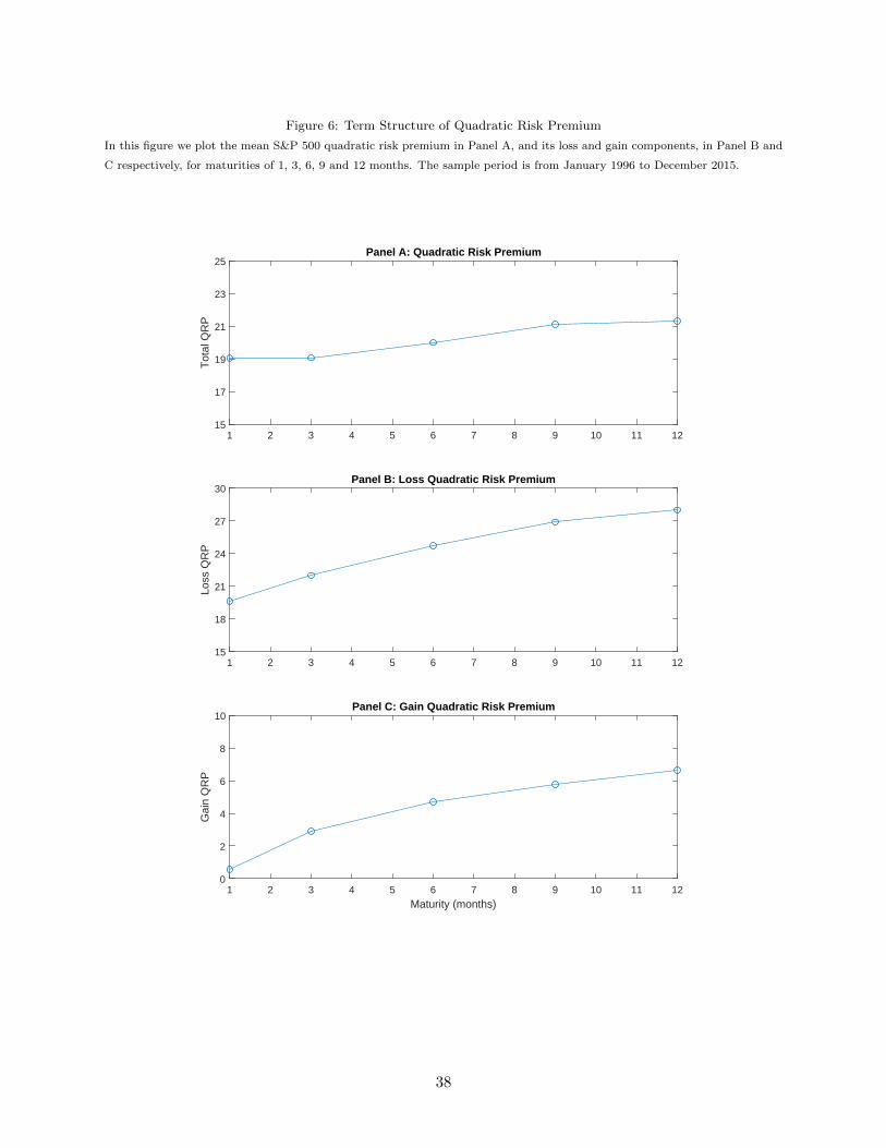
Figure 6: Term Structure of Quadratic Risk Premium

In this figure we plot the mean S&P 500 quadratic risk premium in Panel A, and its loss and gain components, in Panel B and

C respectively, for maturities of 1, 3, 6, 9 and 12 months. The sample period is from January 1996 to December 2015.

1 2 3 4 5 6 7 8 9 10 11 1215

17

19

21

23

25

Tot

al Q

RP

Panel A: Quadratic Risk Premium

1 2 3 4 5 6 7 8 9 10 11 1215

18

21

24

27

30

Loss

QR

P

Panel B: Loss Quadratic Risk Premium

1 2 3 4 5 6 7 8 9 10 11 12

Maturity (months)

0

2

4

6

8

10

Gai

n Q

RP

Panel C: Gain Quadratic Risk Premium

38

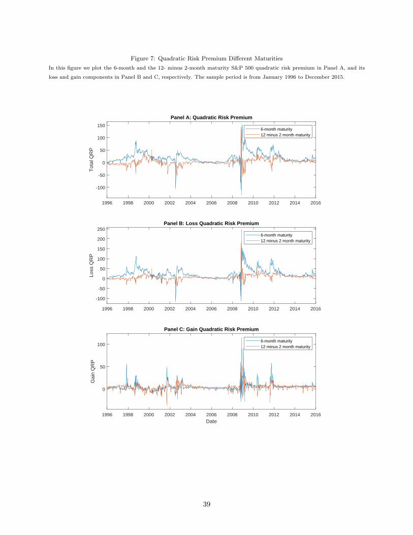
Figure 7: Quadratic Risk Premium Different Maturities

In this figure we plot the 6-month and the 12- minus 2-month maturity S&P 500 quadratic risk premium in Panel A, and its

loss and gain components in Panel B and C, respectively. The sample period is from January 1996 to December 2015.

1996 1998 2000 2002 2004 2006 2008 2010 2012 2014 2016

-100

-50

0

50

100

150

Tot

al Q

RP

Panel A: Quadratic Risk Premium

6-month maturity12 minus 2 month maturity

1996 1998 2000 2002 2004 2006 2008 2010 2012 2014 2016

-100

-50

0

50

100

150

200

250

Loss

QR

P

Panel B: Loss Quadratic Risk Premium

6-month maturity12 minus 2 month maturity

1996 1998 2000 2002 2004 2006 2008 2010 2012 2014 2016

Date

0

50

100

Gai

n Q

RP

Panel C: Gain Quadratic Risk Premium

6-month maturity12 minus 2 month maturity

39

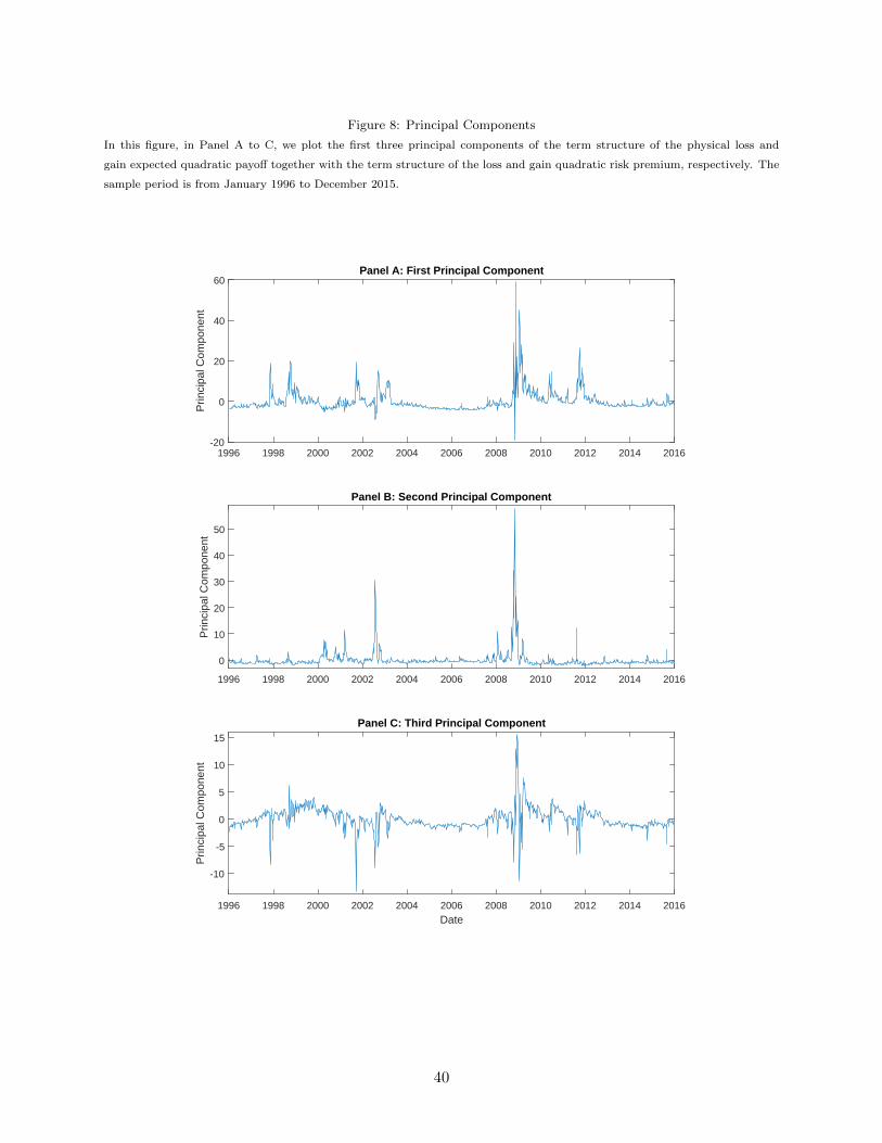
Figure 8: Principal Components

In this figure, in Panel A to C, we plot the first three principal components of the term structure of the physical loss and

gain expected quadratic payoff together with the term structure of the loss and gain quadratic risk premium, respectively. The

sample period is from January 1996 to December 2015.

1996 1998 2000 2002 2004 2006 2008 2010 2012 2014 2016-20

0

20

40

60

Prin

cipa

l Com

pone

nt

Panel A: First Principal Component

1996 1998 2000 2002 2004 2006 2008 2010 2012 2014 2016

0

10

20

30

40

50

Prin

cipa

l Com

pone

nt

Panel B: Second Principal Component

1996 1998 2000 2002 2004 2006 2008 2010 2012 2014 2016

Date

-10

-5

0

5

10

15

Prin

cipa

l Com

pone

nt

Panel C: Third Principal Component

40

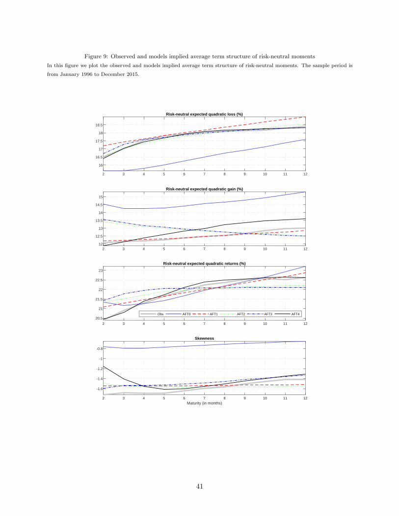
Figure 9: Observed and models implied average term structure of risk-neutral moments

In this figure we plot the observed and models implied average term structure of risk-neutral moments. The sample period is

from January 1996 to December 2015.

2 3 4 5 6 7 8 9 10 11 12

16

16.5

17

17.5

18

18.5

Risk-neutral expected quadratic loss (%)

2 3 4 5 6 7 8 9 10 11 1212

12.5

13

13.5

14

14.5

15

Risk-neutral expected quadratic gain (%)

2 3 4 5 6 7 8 9 10 11 12

20.5

21

21.5

22

22.5

23

Risk-neutral expected quadratic returns (%)

Obs AFT0 AFT1 AFT2 AFT3 AFT4

2 3 4 5 6 7 8 9 10 11 12Maturity (in months)

-1.6

-1.4

-1.2

-1

-0.8

Skewness

41

Figure 10: Observed and models implied average term structure of QRP

Using the most flexible specification of the AFT model (AFT4), in this figure we plot observed and models implied average

loss, gain and total quadratic risk premium. The sample period is from January 1996 to December 2015.

3 6 9 12

-0.02

0

0.02

0.04

0.06

0.08

0.1

Loss QRP

3 6 9 12

-0.01

0

0.01

0.02

0.03

Gain QRP

Obs RND0 RND1 RND2 RND3 RND4

3 6 9 12Maturity (in months)

-0.02

-0.01

0

0.01

0.02

0.03

0.04

0.05

0.06Total QRP

42