Embed Size (px)
Citation preview
THE THEORY OF DEMAND &
SUPPLY
1
DEMAND
Demands for a commodity refers to the quantity of the commodity which an individual consumer is willing to and able to purchase per unit of time at a particular price.
2
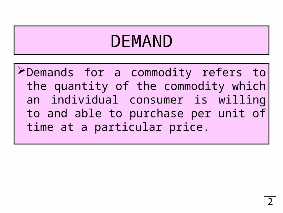
DETERMINANTS OF DEMAND Price of the commodity Price of Related Goods and Services Consumer’s Income Consumer’s Taste & Preferences Distribution of Income Expectations Sociological Variables Demonstration Effect & Band –Wagon Effect
3
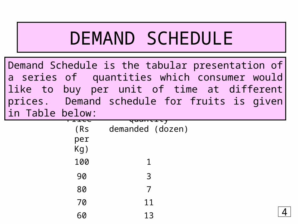
Demand Schedule for Fruit by an Individual
Price (Rs per
Kg)
Quantitydemanded (dozen)
100 1
90 3
80 7
70 11
60 13
Demand Schedule is the tabular presentation of a series of quantities which consumer would like to buy per unit of time at different prices. Demand schedule for fruits is given in Table below:
DEMAND SCHEDULE
4
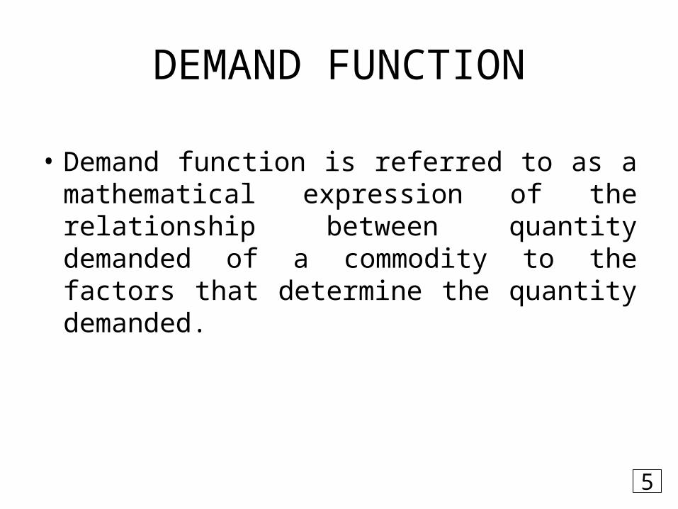
DEMAND FUNCTION
• Demand function is referred to as a mathematical expression of the relationship between quantity demanded of a commodity to the factors that determine the quantity demanded.
5
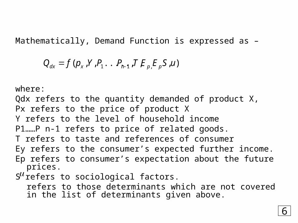
Mathematically, Demand Function is expressed as –
where:Qdx refers to the quantity demanded of product X,Px refers to the price of product XY refers to the level of household incomeP1……P n-1 refers to price of related goods.T refers to taste and references of consumerEy refers to the consumer’s expected further income.Ep refers to consumer’s expectation about the future prices.S refers to sociological factors.
refers to those determinants which are not covered in the list of determinants given above.
),,,......,,( ,11 uSEETPPYpfQ ppnxdx
6
THE LAW OF DEMAND
• The law of demand holds that other things equal, as the price of a good or service rises, its quantity demanded falls.– The reverse is also true: as the price of a
good or service falls, its quantity demanded increases.
7
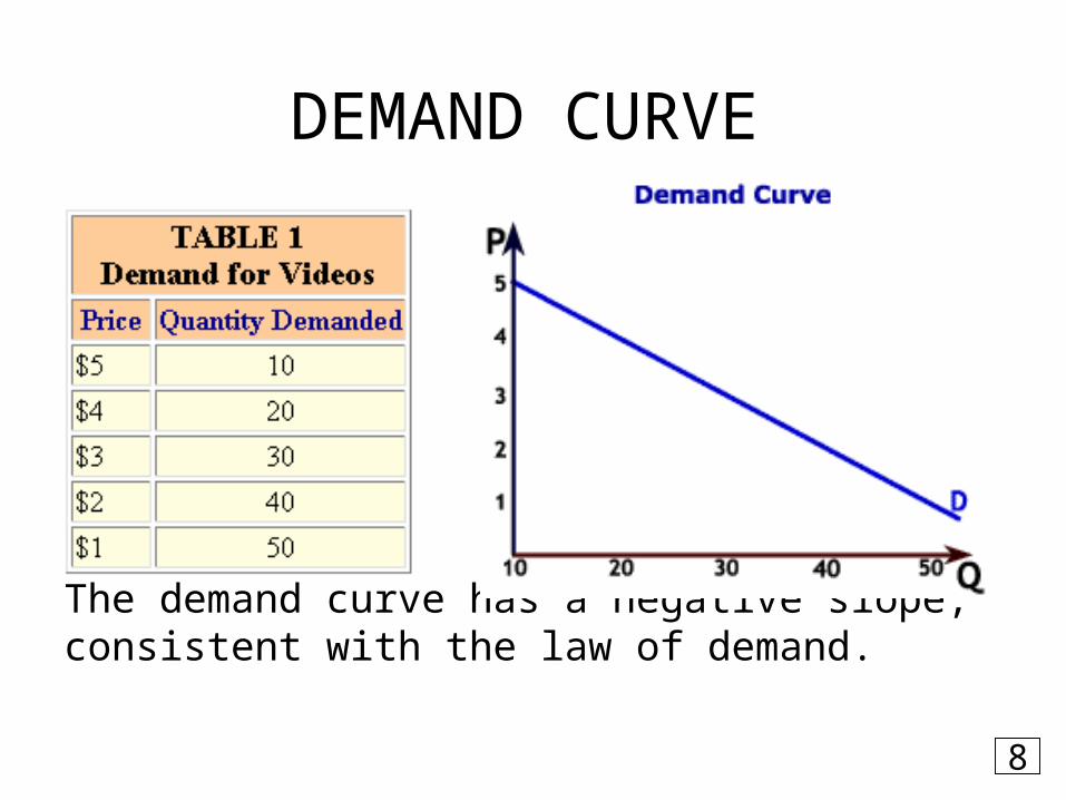
DEMAND CURVE
The demand curve has a negative slope, consistent with the law of demand.
8
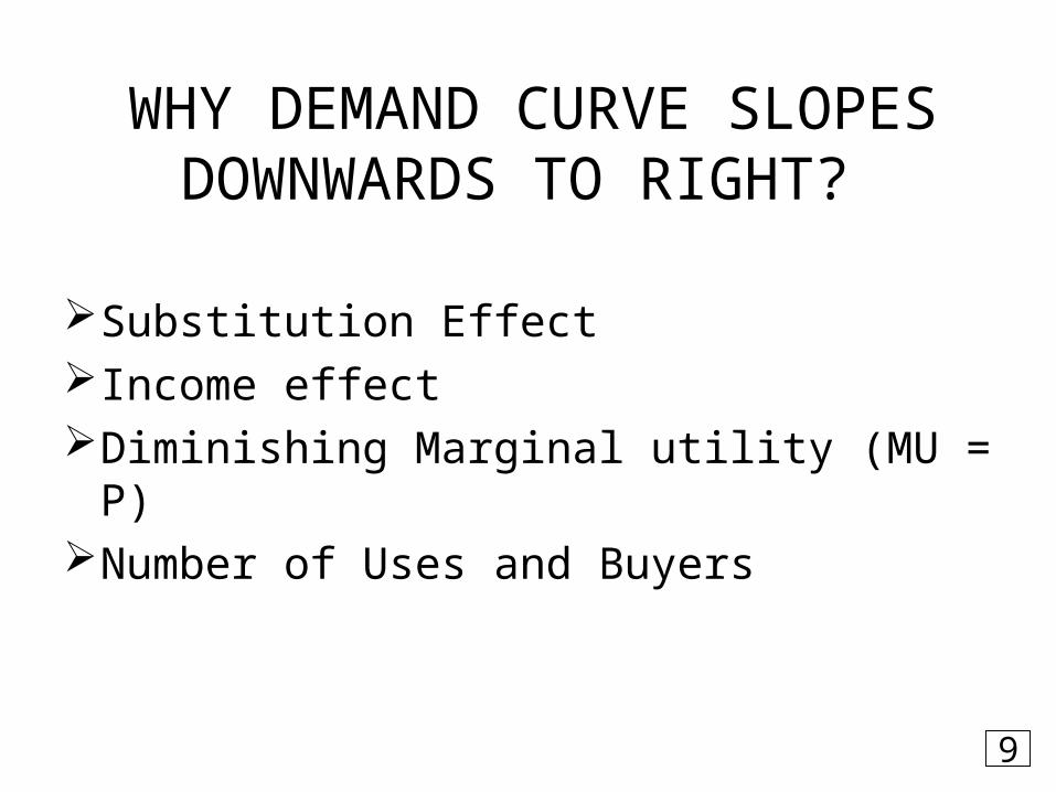
WHY DEMAND CURVE SLOPES DOWNWARDS TO RIGHT?
Substitution Effect Income effect Diminishing Marginal utility (MU = P)Number of Uses and Buyers
9

EXCEPTIONS TO LAW OF DEMAND
Giffen Goods Status Goods Expectation of future price Emergencies Ignorance
10
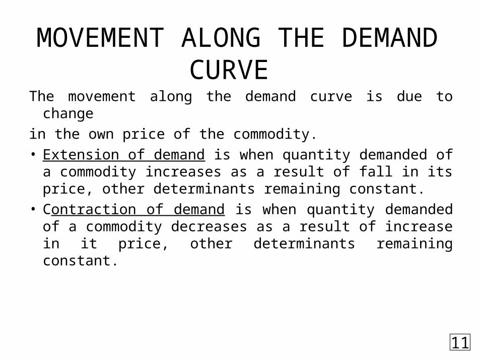
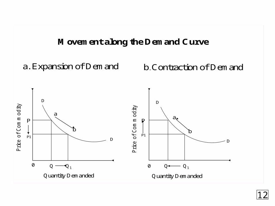
MOVEMENT ALONG THE DEMAND CURVE
The movement along the demand curve is due to change
in the own price of the commodity.• Extension of demand is when quantity demanded of
a commodity increases as a result of fall in its price, other determinants remaining constant.
• Contraction of demand is when quantity demanded of a commodity decreases as a result of increase in it price, other determinants remaining constant.
11
D
D
0 Q Q1
a
b
Price
of Com
modity
P
P1
Quantity Demanded
Movement along the Demand Curve
a. Expansion of Demand b. Contraction of Demand
Quantity Demanded
D
D
Price
of Com
modity
P
P1
a
b
0 Q Q1
12

SHIFT IN THE DEMAND CURVE• A change in any variable other than price that
influences quantity demanded produces a shift in the demand curve or a change in demand.
• Factors that shift the demand curve include:– Change in consumer incomes– Population change– Consumer preferences– Prices of related goods:
• Substitutes: goods consumed in place of one another• Complements: goods consumed jointly
13
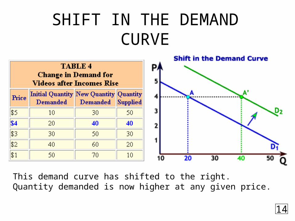
SHIFT IN THE DEMAND CURVE
This demand curve has shifted to the right. Quantity demanded is now higher at any given price.
14
TYPES OF DEMAND
• Direct/Autonomous Demand and Derived Demand
• Non Durables Goods Demand and Durable Goods Demand
• Industry Demand and Individual Firm Demand
• Short Run Demand and Long-Run Demand
15

SUPPLY
Supply of a commodity refers to the various quantities of the commodity which a seller is willing and able to sell at different prices, in a given market, at a point of time, other things remaining the same.
16
DETERMINANTS OF SUPPLY
Price Price of related goods Cost of Production/Factors of Production State of Technology Goal of Producer Natural factors Other Factors
17
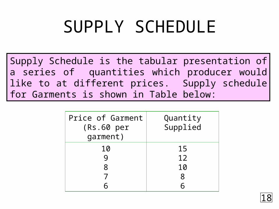
SUPPLY SCHEDULE
Supply Schedule is the tabular presentation of a series of quantities which producer would like to at different prices. Supply schedule for Garments is shown in Table below:
Price of Garment(Rs.60 per garment)
Quantity Supplied
109876
15121086
18
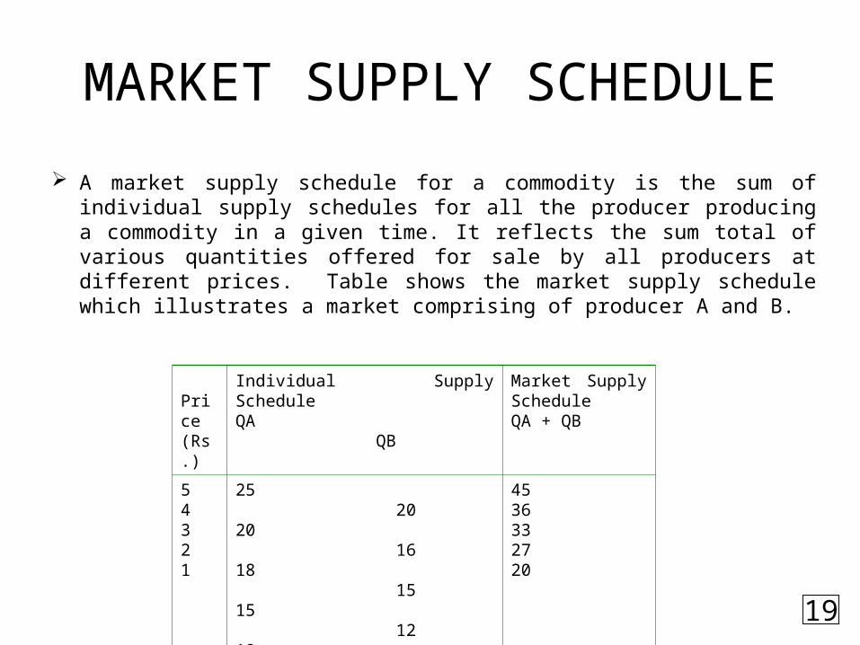
MARKET SUPPLY SCHEDULE
A market supply schedule for a commodity is the sum of individual supply schedules for all the producer producing a commodity in a given time. It reflects the sum total of various quantities offered for sale by all producers at different prices. Table shows the market supply schedule which illustrates a market comprising of producer A and B.
Price (Rs.)
Individual Supply ScheduleQA QB
Market Supply ScheduleQA + QB
54321
25 2020 1618 1515 1210 10
4536332720
19
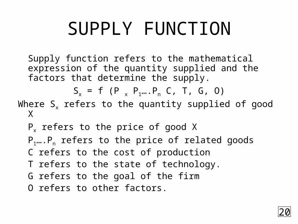
SUPPLY FUNCTION
Supply function refers to the mathematical expression of the quantity supplied and the factors that determine the supply.
Sx = f (P x P1….Pn C, T, G, O)
Where Sx refers to the quantity supplied of good X
Px refers to the price of good X
P1….Pn refers to the price of related goodsC refers to the cost of productionT refers to the state of technology.G refers to the goal of the firmO refers to other factors.
20
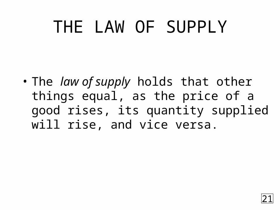
THE LAW OF SUPPLY
• The law of supply holds that other things equal, as the price of a good rises, its quantity supplied will rise, and vice versa.
21

WHY IS SUPPLY CURVE AN UPWARD SLOPING CURVE?
• Profit Maximization
• The Law of Diminishing Marginal Productivity
22
23
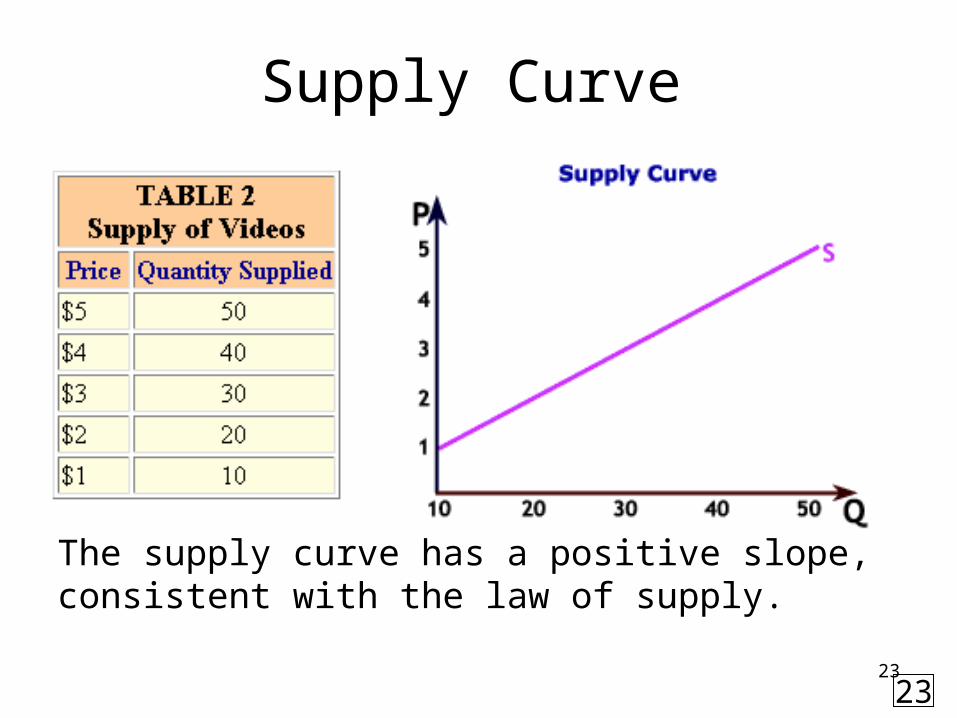
Supply Curve
The supply curve has a positive slope, consistent with the law of supply.
23
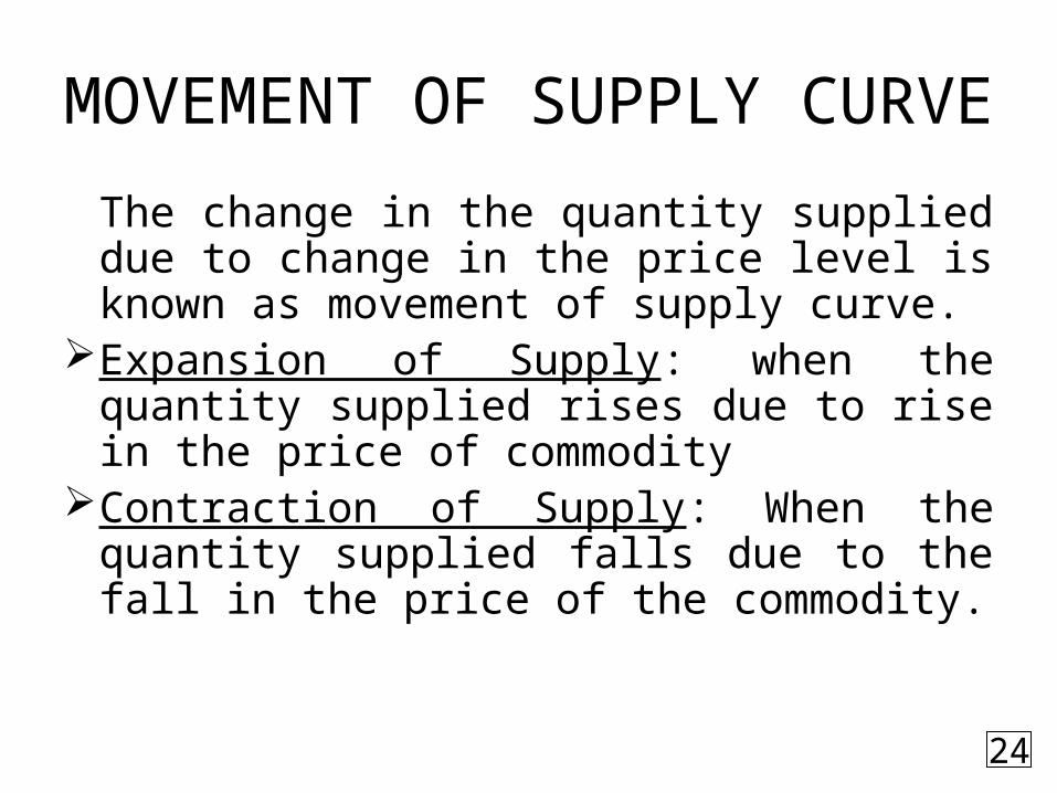
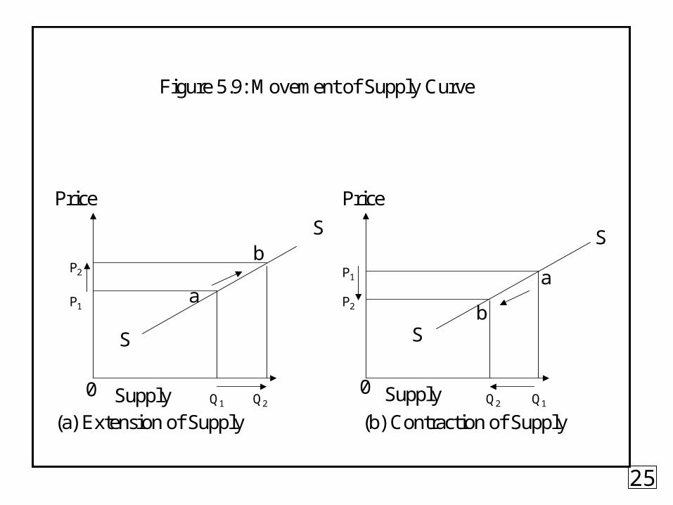
MOVEMENT OF SUPPLY CURVE
The change in the quantity supplied due to change in the price level is known as movement of supply curve.
Expansion of Supply: when the quantity supplied rises due to rise in the price of commodity
Contraction of Supply: When the quantity supplied falls due to the fall in the price of the commodity.
24
S S
SS
P2
P1
Price
b
a P2
Q2 Q2
P1
Q1 Q1
a
b
Price
0 0
Figure 5.9: Movement of Supply Curve
(a) Extension of Supply (b) Contraction of SupplySupply Supply
25
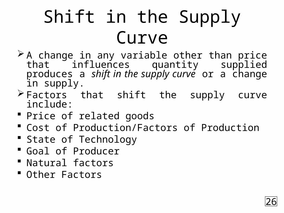
Shift in the Supply Curve
A change in any variable other than price that influences quantity supplied produces a shift in the supply curve or a change in supply.
Factors that shift the supply curve include: Price of related goods Cost of Production/Factors of Production State of Technology Goal of Producer Natural factors Other Factors
26
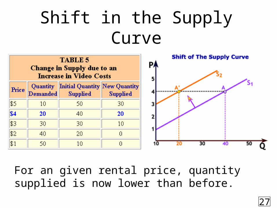
Shift in the Supply Curve
For an given rental price, quantity supplied is now lower than before.
27
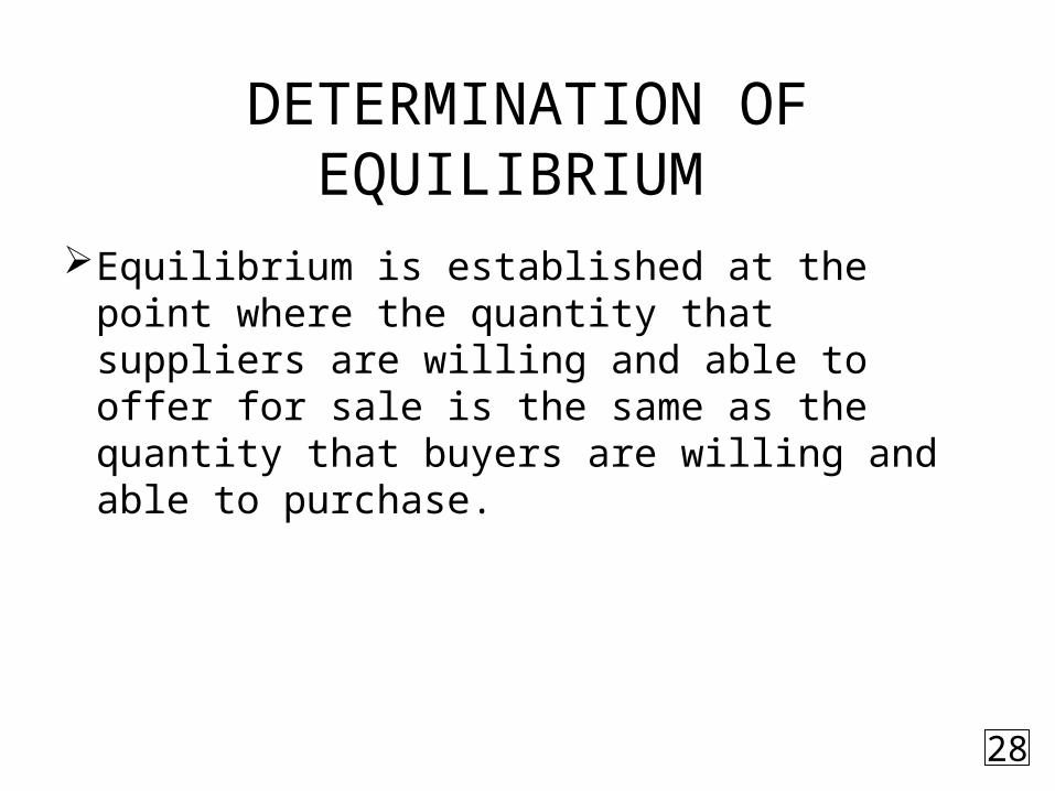
DETERMINATION OF EQUILIBRIUM
Equilibrium is established at the point where the quantity that suppliers are willing and able to offer for sale is the same as the quantity that buyers are willing and able to purchase.
28

EQUILIBRIUM
Equilibrium occurs at a price of $3 and a quantity of 30 units.
29
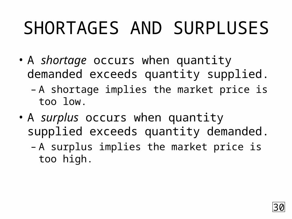
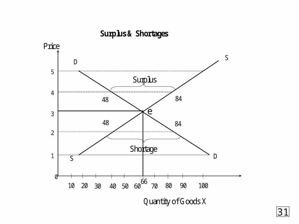
SHORTAGES AND SURPLUSES
• A shortage occurs when quantity demanded exceeds quantity supplied.– A shortage implies the market price is too low.
• A surplus occurs when quantity supplied exceeds quantity demanded. – A surplus implies the market price is too high.
30
0
Surplus
Shortage
Surplus & Shortages
Price
Quantity of Goods X
1
2
3
4
5
10 7066
80 90 10020 30 40 50 60
48
48
84
84
e
S
S
D
D
31
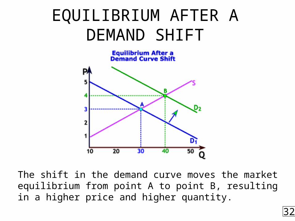
EQUILIBRIUM AFTER A DEMAND SHIFT
The shift in the demand curve moves the market equilibrium from point A to point B, resulting in a higher price and higher quantity.
32
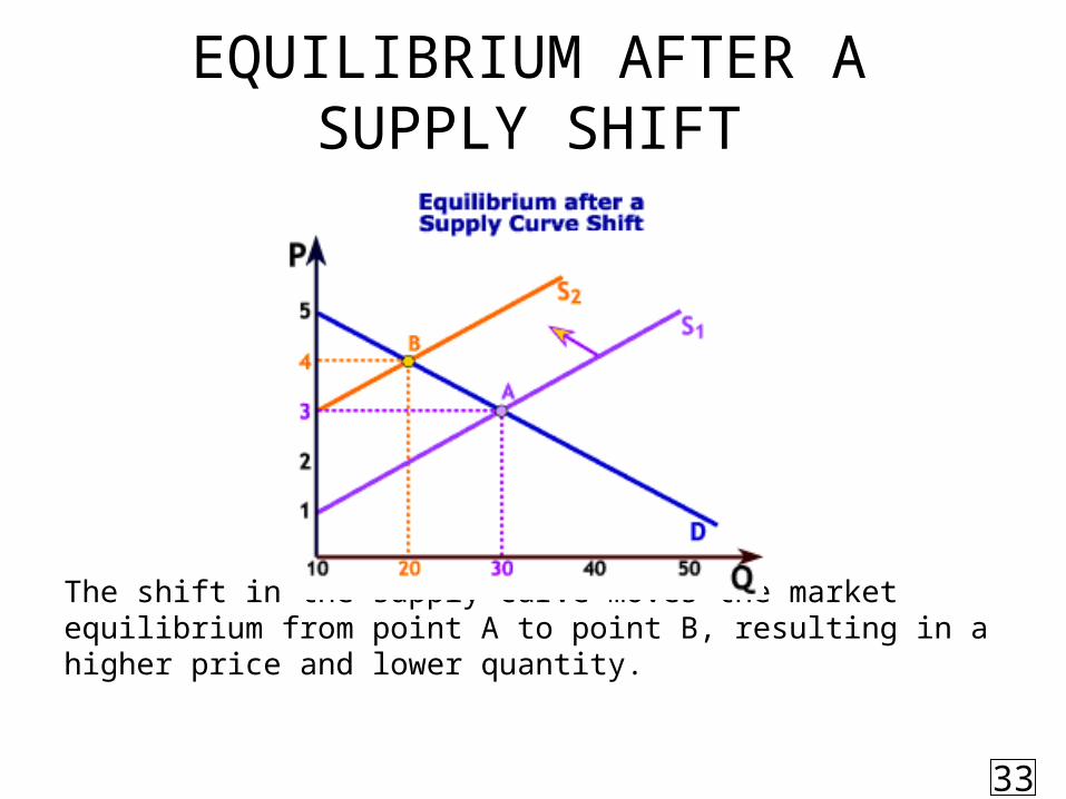
EQUILIBRIUM AFTER A SUPPLY SHIFT
The shift in the supply curve moves the market equilibrium from point A to point B, resulting in a higher price and lower quantity.
33
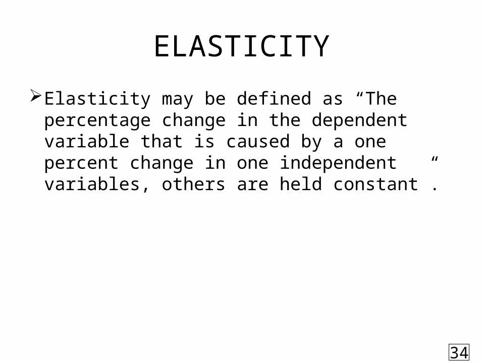
ELASTICITY
Elasticity may be defined as “The percentage change in the dependent variable that is caused by a one percent change in one independent variables, others are held constant”.
34

ELASTICITY OF DEMAND
Elasticity of demand measures degree of responsiveness of the quantity demanded to change in any one of the factors that influence it.
Ed = Percentage change in quantity demanded of good X
Percentage change in determinant Y
35
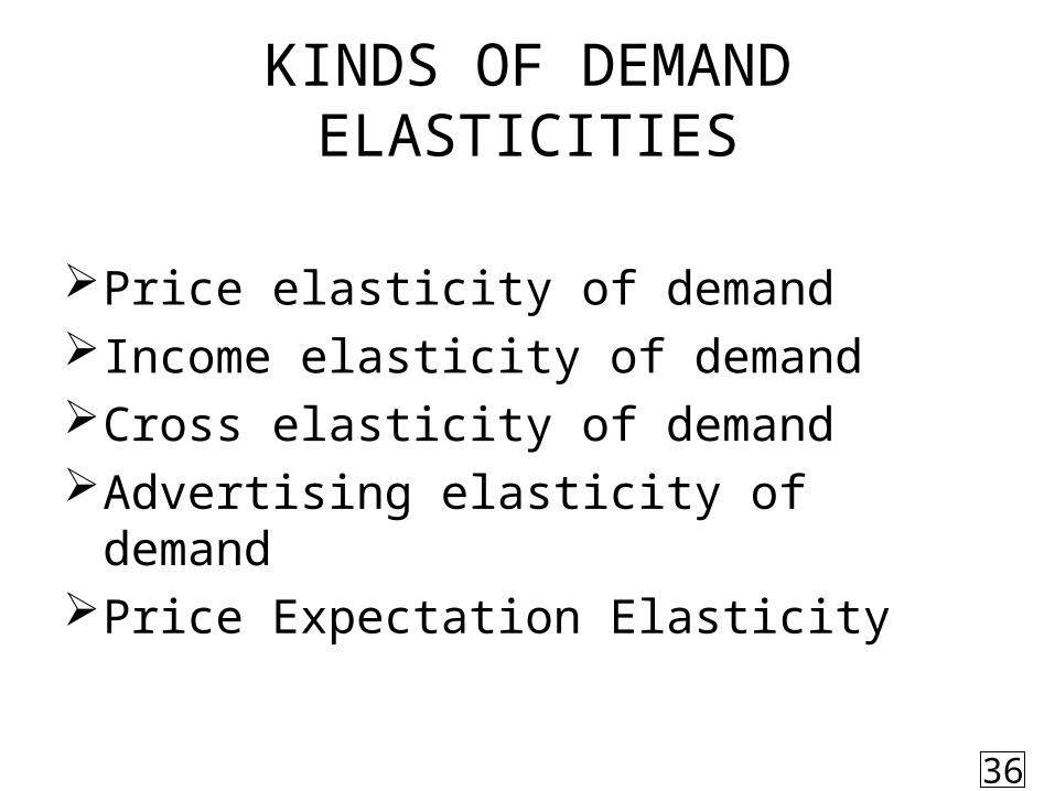
KINDS OF DEMAND ELASTICITIES
Price elasticity of demandIncome elasticity of demandCross elasticity of demandAdvertising elasticity of demandPrice Expectation Elasticity
36
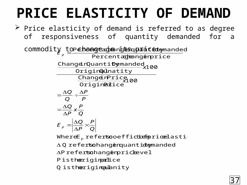
PRICE ELASTICITY OF DEMAND Price elasticity of demand is referred to as degree of responsiveness
of quantity demanded for a commodity to change in its price
quanity original theis Q
price original theis P
level pricein change torefers P
demandedquantity in change torefers Q
elasticity price oft coefficien torefers E Where
100 Price Original
Pricein Change
100Qunatity Original
DemandedQuantity in Change
pricein change Percentage
demandedquantity in change Percentage
p
Q
P
P
QE
Q
Px
P
Q
P
P
Q
Q
x
x
E
p
p
37
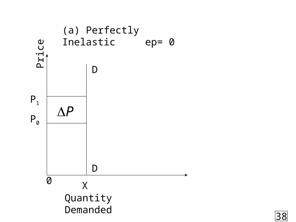
0
D
Quantity Demanded
Pri
ce
PP0
X
P1
D
(a) Perfectly Inelastic ep= 0
38
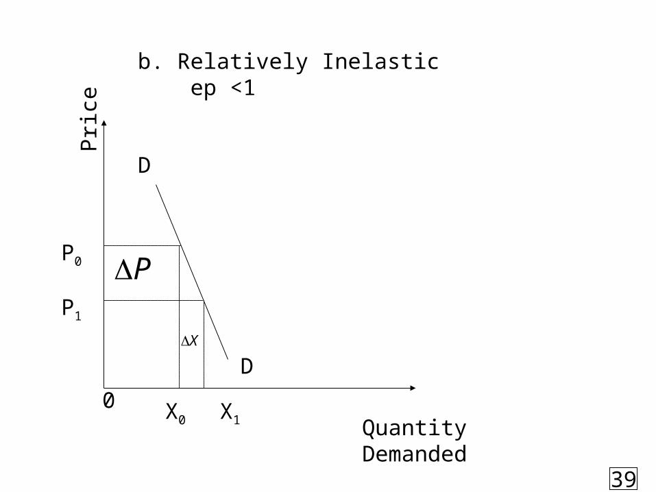
0 X0
D
Quantity Demanded
Pri
ce
P
D
P1
P0
X1
X
b. Relatively Inelastic ep <1
39
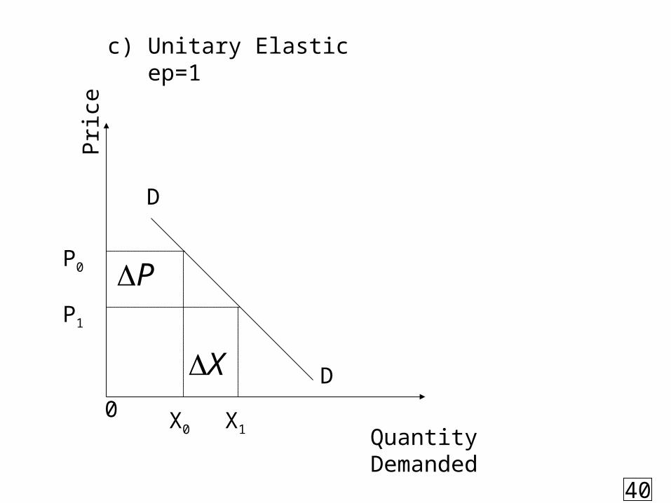
0 X0
D
Quantity Demanded
Pri
ce
P
X D
P1
P0
X1
c) Unitary Elastic ep=1
40
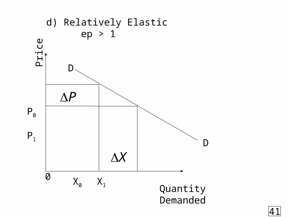
0 X0
D
Quantity Demanded
Pri
ce
P1
P0
X1
D
P
X
d) Relatively Elastic ep > 1
41
0 X0
D
Quantity Demanded
Pri
ce
X
P0
X1
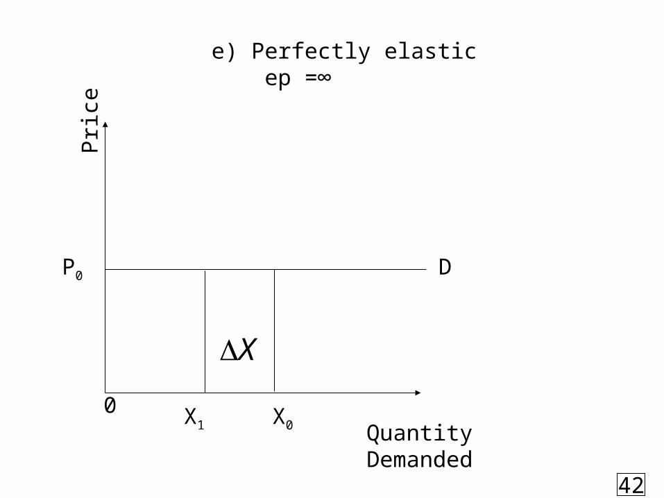
e) Perfectly elastic ep =∞
42
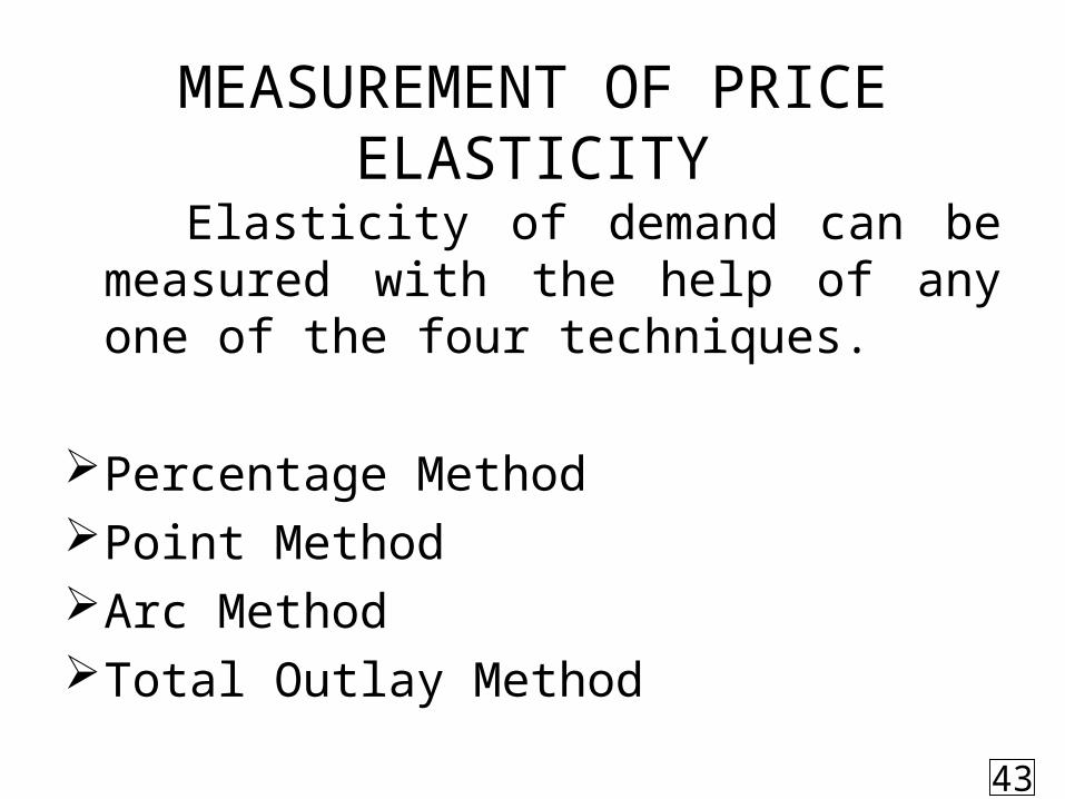
MEASUREMENT OF PRICE ELASTICITY
Elasticity of demand can be measured with the help of any one of the four techniques.
Percentage MethodPoint MethodArc MethodTotal Outlay Method
43
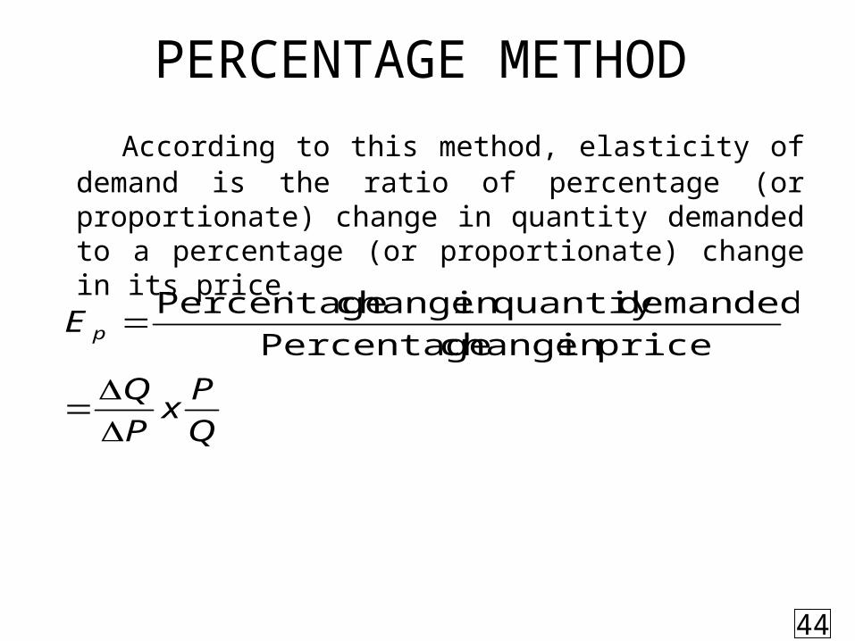
PERCENTAGE METHOD
According to this method, elasticity of demand is the ratio of percentage (or proportionate) change in quantity demanded to a percentage (or proportionate) change in its price.
Q
Px
P
Q
E p
pricein change Percentage
demandedquantiy in change Percentage
44
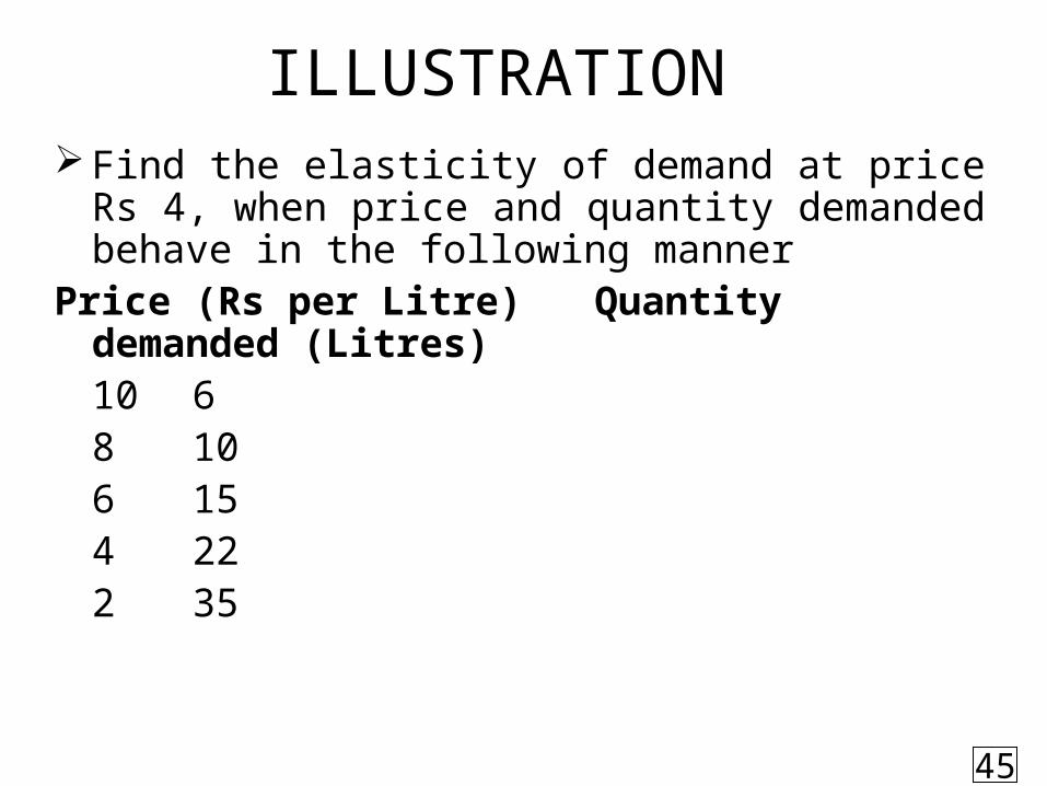
ILLUSTRATION Find the elasticity of demand at price Rs 4, when
price and quantity demanded behave in the following manner
Price (Rs per Litre) Quantity demanded (Litres)
10 68 106 154 222 35
45
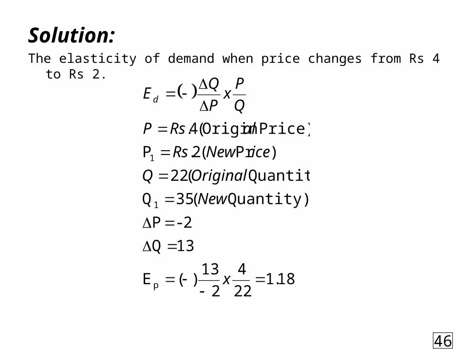
Solution:The elasticity of demand when price changes from Rs 4 to Rs 2.
18.122
4
2
13)(E
13 Q
2- P
Quantity) (35Q
Quantity) (22
)Pr(2.P
Price) Origin(4.
p
1
1
x
New
OriginalQ
iceNewRs
alRsP
Q
Px
P
QEd
46
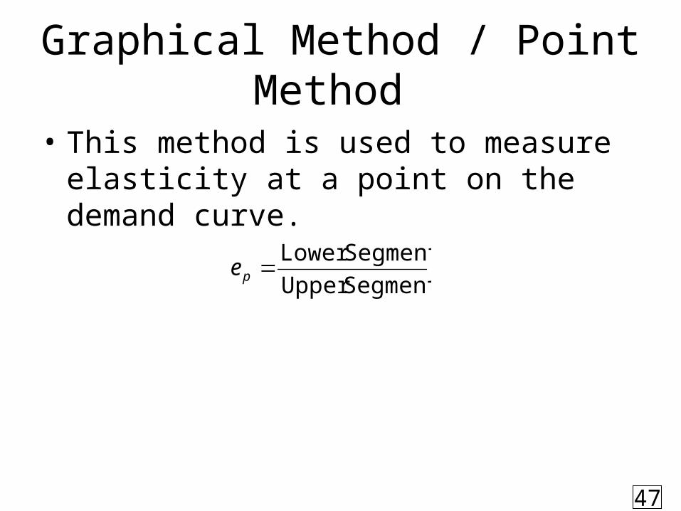
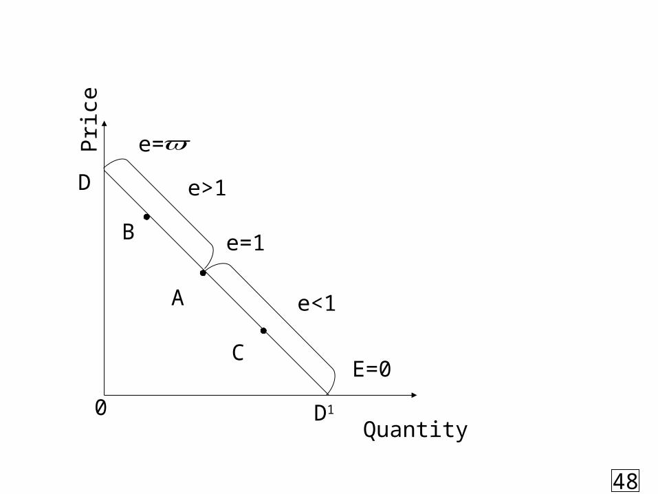
Graphical Method / Point Method
• This method is used to measure elasticity at a point on the demand curve.
SegmentUpper
SegmentLower pe
47
0 D1
D
Quantity
Pri
ce
e=
e=1
e<1
E=0
B
A
C
e>1
48
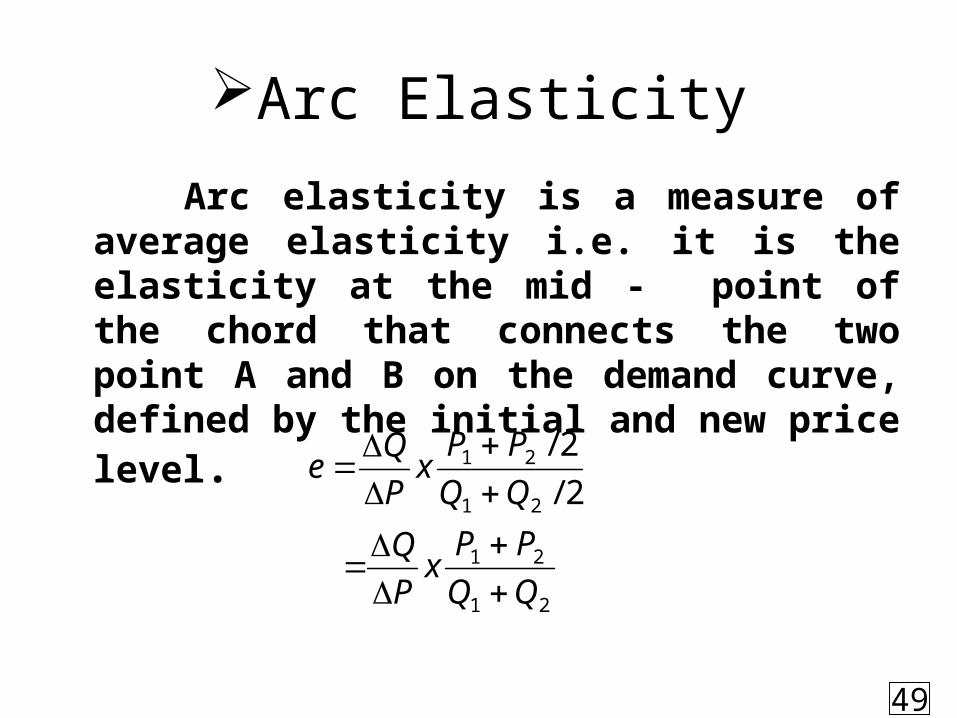
Arc Elasticity
Arc elasticity is a measure of average elasticity i.e. it is the elasticity at the mid - point of the chord that connects the two point A and B on the demand curve, defined by the initial and new price level.
21
21
21
21
2/
2/
PPx
P
Q
PPx
P
Qe
49
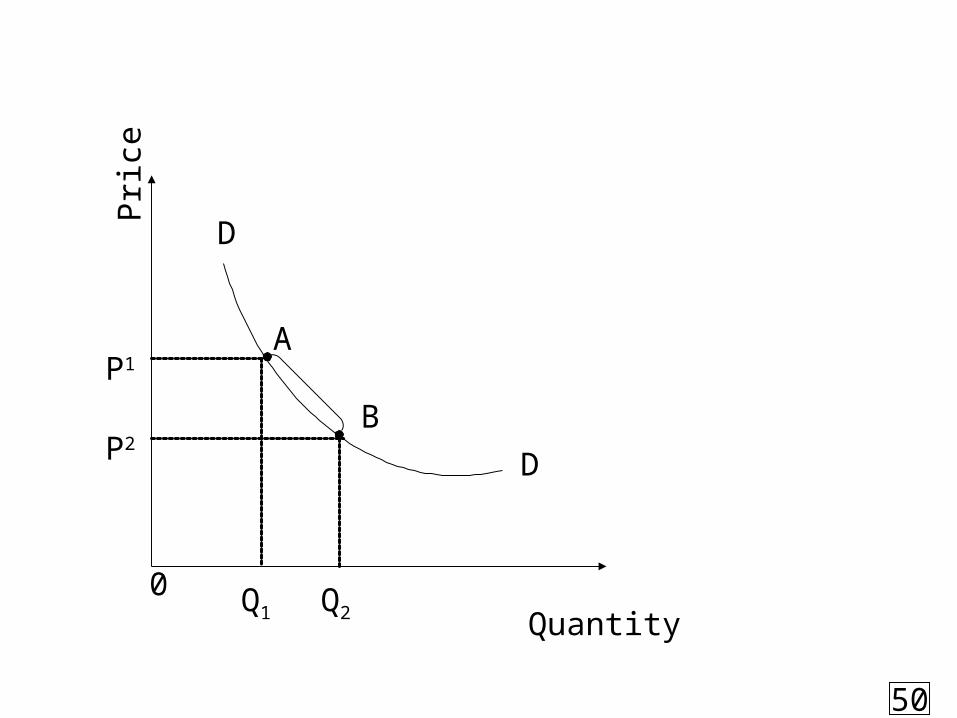
A
B
P1
0 Q1 Q2 Quantity
Pri
ce
D
D
P2
50
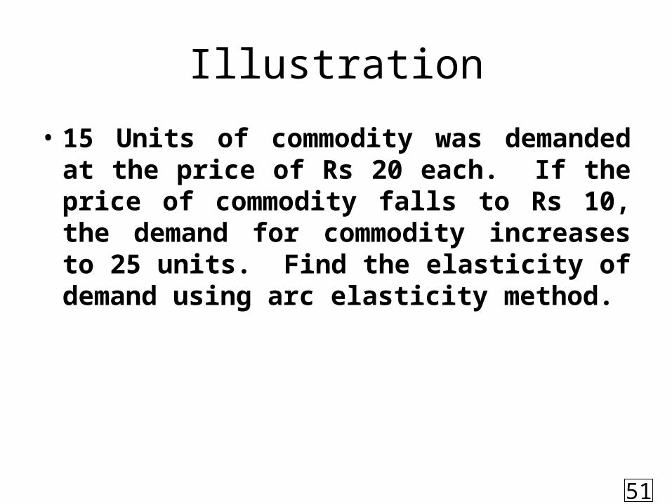
Illustration
• 15 Units of commodity was demanded at the price of Rs 20 each. If the price of commodity falls to Rs 10, the demand for commodity increases to 25 units. Find the elasticity of demand using arc elasticity method.
51
• Solution:
75.4
3
40
30
10
10e
10 Q 10- P
25 Q 10
15Q 20P
p
22
11
21
21
P
units
PP
P
Qe p
52
TOTAL OUTLAY METHOD/EXPRENDITURE METHOD
In this method, we study the elasticity of demand in relation to change in total outlay (expenditure) as a result of change in price and the consequent change in demand for a product.
Limitation: It does not give the precise value of the elasticity of demand, rather it only tells whether the elasticity is equal to one, greater than one or less than one.
53
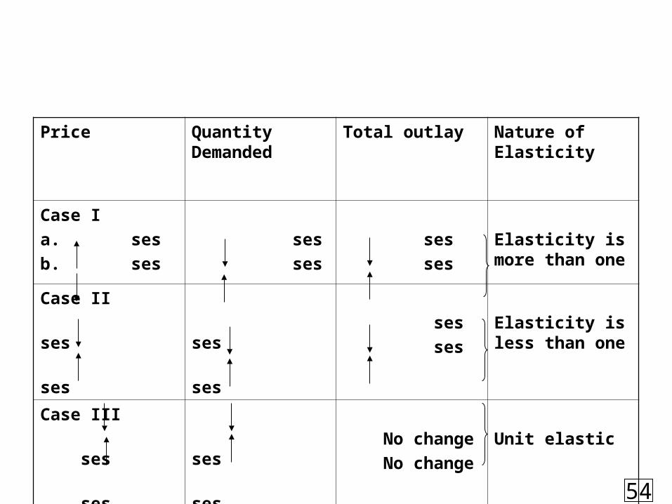
Price Quantity Demanded
Total outlay Nature of Elasticity
Case I
a. ses
b. ses
ses
ses
ses
ses
Elasticity is more than one
Case II
ses
ses
ses
ses
ses
ses
Elasticity is less than one
Case III
ses
ses
ses
ses
No change
No change
Unit elastic
54
FACTORS AFFECTING ELASTICITY OF DEMAND
• Nature of Commodity
• Number of close substitutes available
• The Proportion of Buyer’s Budget
• Number of uses of Commodity
• Consumer’s Behaviour
• Price Level of the Commodity
• Time Period
55
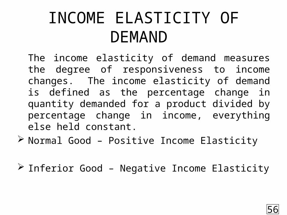
INCOME ELASTICITY OF DEMAND
The income elasticity of demand measures the degree of responsiveness to income changes. The income elasticity of demand is defined as the percentage change in quantity demanded for a product divided by percentage change in income, everything else held constant.
Normal Good – Positive Income Elasticity
Inferior Good – Negative Income Elasticity
56
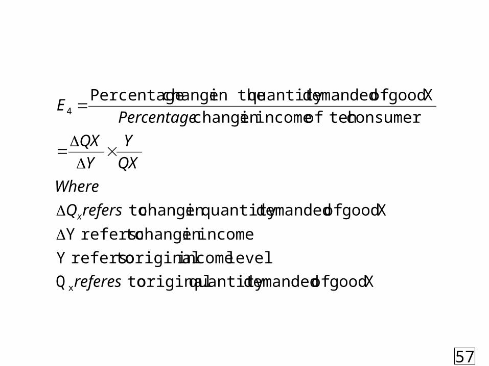
X good of demandedquantity original toQ
level income original torefers Y
incomein change torefers Y
X good of demandedquantity in change to
consumer teh of incomein change
X good of demandedquantity in the change Percentage
x
4
referes
refersQ
Where
QX
Y
Y
QX
PercentageE
x
57
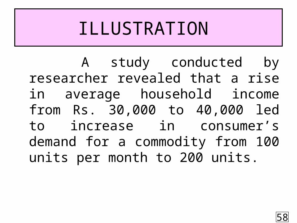
A study conducted by researcher revealed that a rise in average household income from Rs. 30,000 to 40,000 led to increase in consumer’s demand for a commodity from 100 units per month to 200 units.
ILLUSTRATION
58
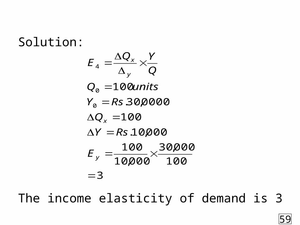
Solution:
The income elasticity of demand is 3
3
100
000,30
000,10
100
000,10.
100
0000,30.
100
0
0
4
y
x
y
x
E
RsY
Q
RsY
unitsQ
Q
YQE
59
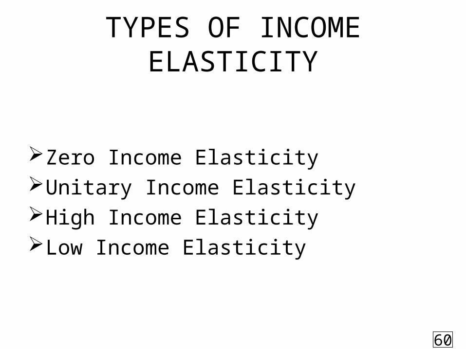
TYPES OF INCOME ELASTICITY
Zero Income ElasticityUnitary Income ElasticityHigh Income ElasticityLow Income Elasticity
60
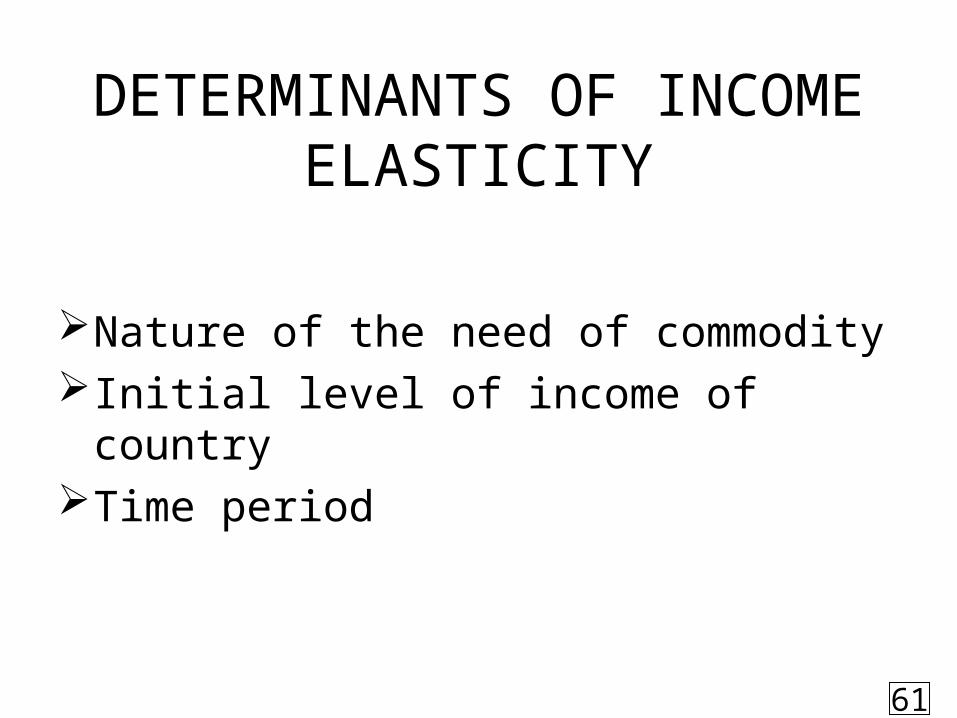
DETERMINANTS OF INCOME ELASTICITY
Nature of the need of commodityInitial level of income of countryTime period
61
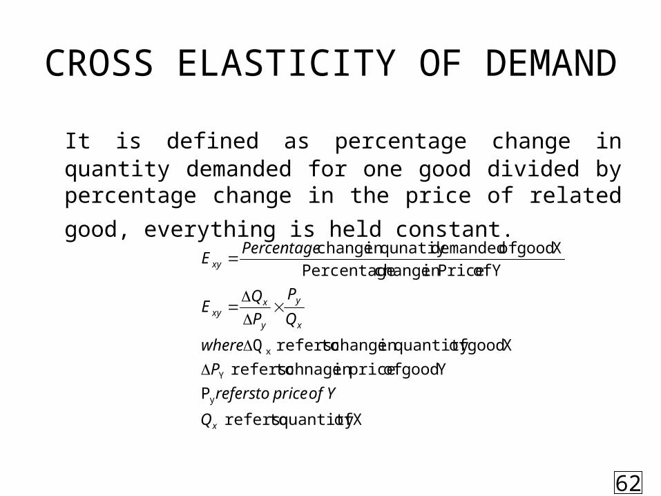
CROSS ELASTICITY OF DEMAND
It is defined as percentage change in quantity demanded for one good divided by percentage change in the price
of related good, everything is held constant.
X ofquantity torefers
P
Y good of pricein chnage torefers
X good ofquantity in change torefers Q
Y of Pricein change Percentage
X good of demandedqunatiy in change
y
Y
x
x
x
y
y
xxy
xy
Q
Yofpricetorefers
P
where
Q
P
P
QE
PercentageE
62
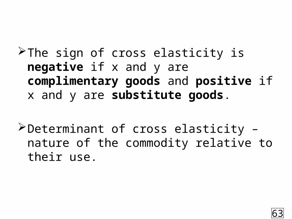
The sign of cross elasticity is negative if x and y are complimentary goods and positive if x and y are substitute goods.
Determinant of cross elasticity – nature of the commodity relative to their use.
63
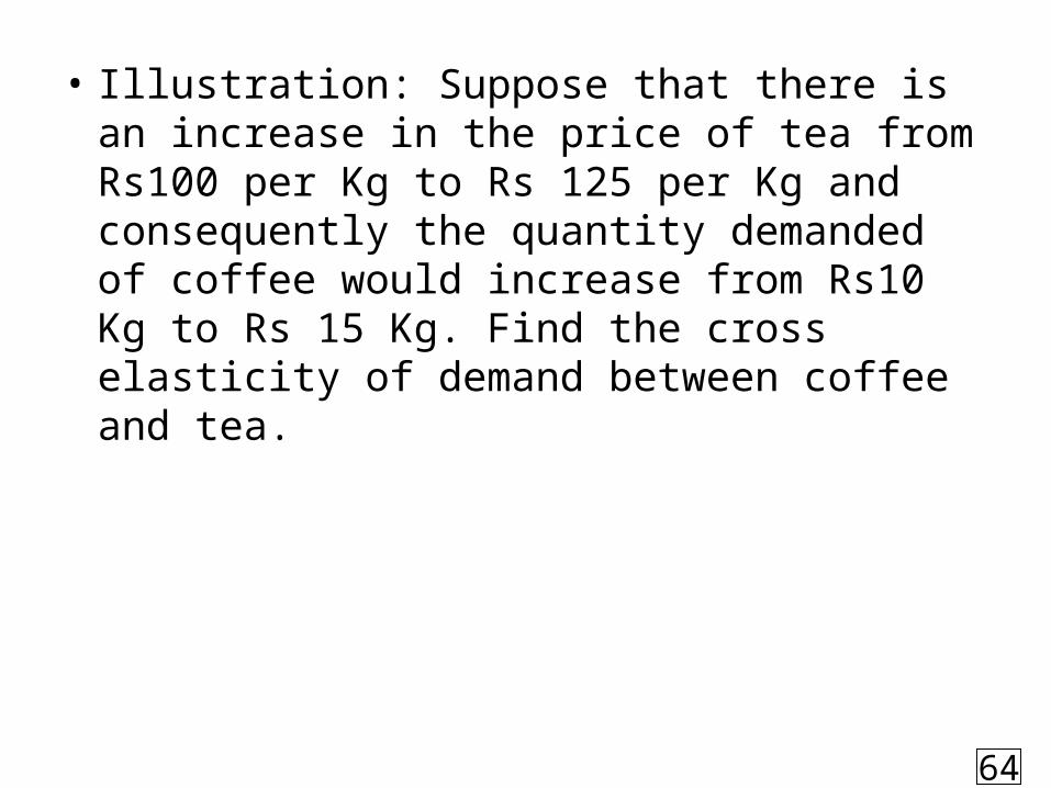
• Illustration: Suppose that there is an increase in the price of tea from Rs100 per Kg to Rs 125 per Kg and consequently the quantity demanded of coffee would increase from Rs10 Kg to Rs 15 Kg. Find the cross elasticity of demand between coffee and tea.
64
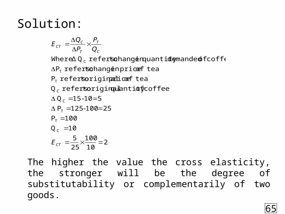
Solution:
The higher the value the cross elasticity, the stronger will be the degree of substitutability or complementarily of two goods.
210
100
25
5
10 Q
100 P
25 100-125 P
5 10-15 Q
coffee ofquantity original torefers Q
teaof price original torefers P
teaof pricein change torefers P
coffee of demandedquantity in change torefers Q Δ Where
C
T
T
C
C
T
T
C
CT
C
T
T
CCT
E
Q
P
P
QE
65
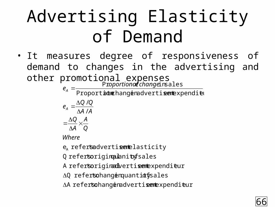
Advertising Elasticity of Demand
• It measures degree of responsiveness of demand to changes in the advertising and other promotional expenses
eexpenditurent advertisemin change torefersA
sales ofquantity in change torefers Q
eexpenditurent advertisem original torefersA
sales ofquanity original torefers Q
elasticityent advertisem torefers e
/
/
eexpenditurent advertisemin change ateProportion
salesin Pr
A
Where
Q
A
A
QAA
QQe
changeeoportionate
A
A
66

Determinants of advertisement elasticity
Kind of productStage of product’s developmentTarget customersQuantity and quality of advertisementReaction of rival firm
67
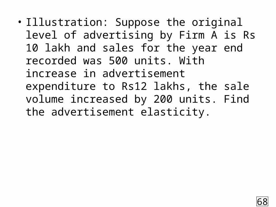
• Illustration: Suppose the original level of advertising by Firm A is Rs 10 lakh and sales for the year end recorded was 500 units. With increase in advertisement expenditure to Rs12 lakhs, the sale volume increased by 200 units. Find the advertisement elasticity.
68
Solution
Original level of advertising = Rs. 10 Lakh
Original quantity = 500 units
New level of addressing = Rs. 12 lakh
New Quantity = 700 units
Therefore, the advertising elasticity of demand is 2, which is termed as relatively elastic. In other words, a 1% increase in the level of advertising will cause a 2 % increase in quantity demanded.
2500
10
2
200
Q
A
A
QeA
69
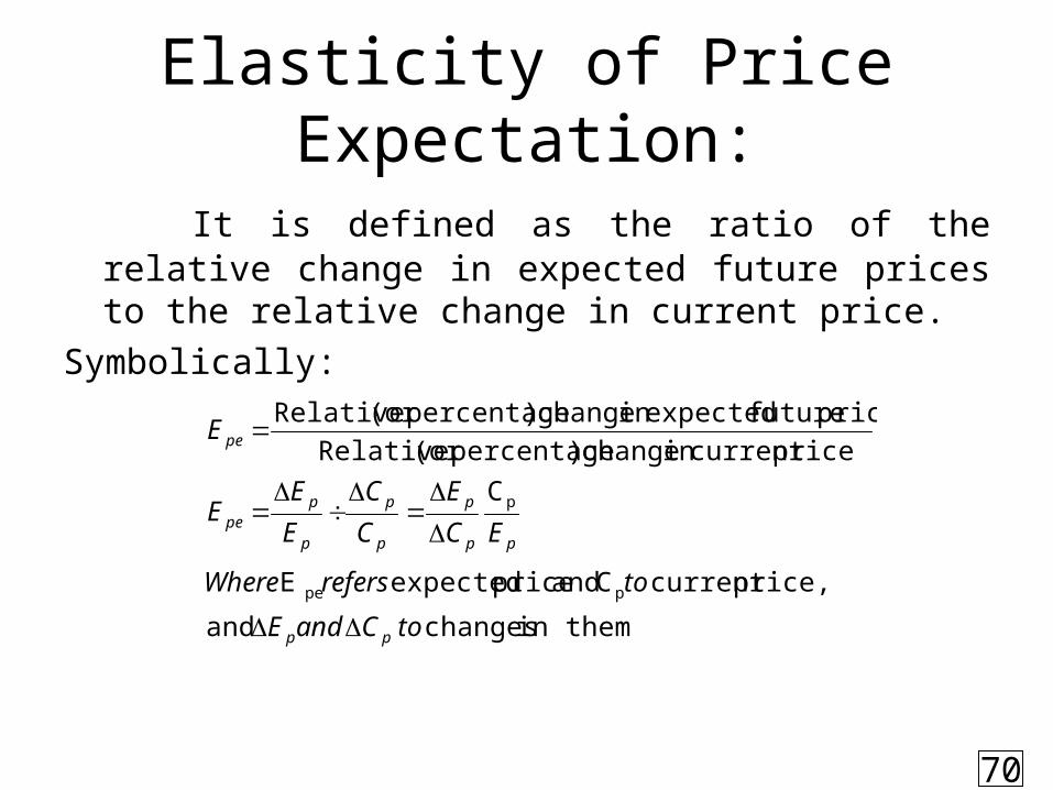
Elasticity of Price Expectation:
It is defined as the ratio of the relative change in expected future prices to the relative change in current price.
Symbolically:
in them changes and
price,current C and price expected E
C
pricecurrent in change )percentage(or Relative
price future expectedin change )percentage(or Relative
ppe
p
toCandE
torefersWhere
EC
E
C
C
E
EE
E
pp
pp
p
p
p
p
ppe
pe
70
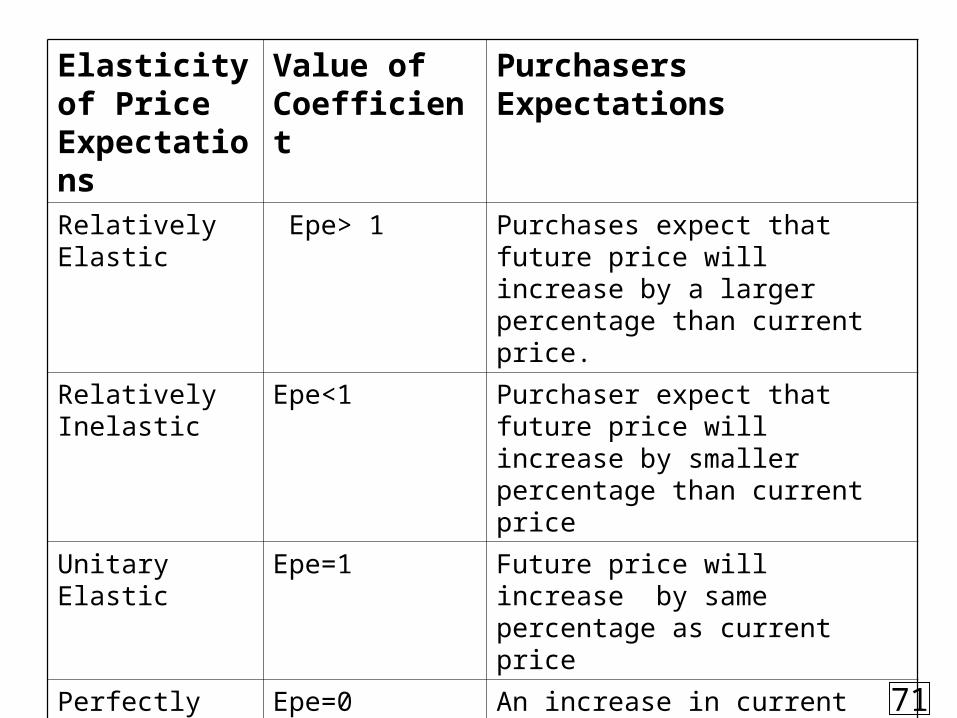
Elasticity of Price Expectations
Value of Coefficient
Purchasers Expectations
Relatively Elastic
Epe> 1 Purchases expect that future price will increase by a larger percentage than current price.
Relatively Inelastic
Epe<1 Purchaser expect that future price will increase by smaller percentage than current price
Unitary Elastic Epe=1 Future price will increase by same percentage as current price
Perfectly Inelastic
Epe=0 An increase in current price will have no effect on future price
Perfectly Elastic Epe=∞ Increase in current price will be followed by decrease in future price
71
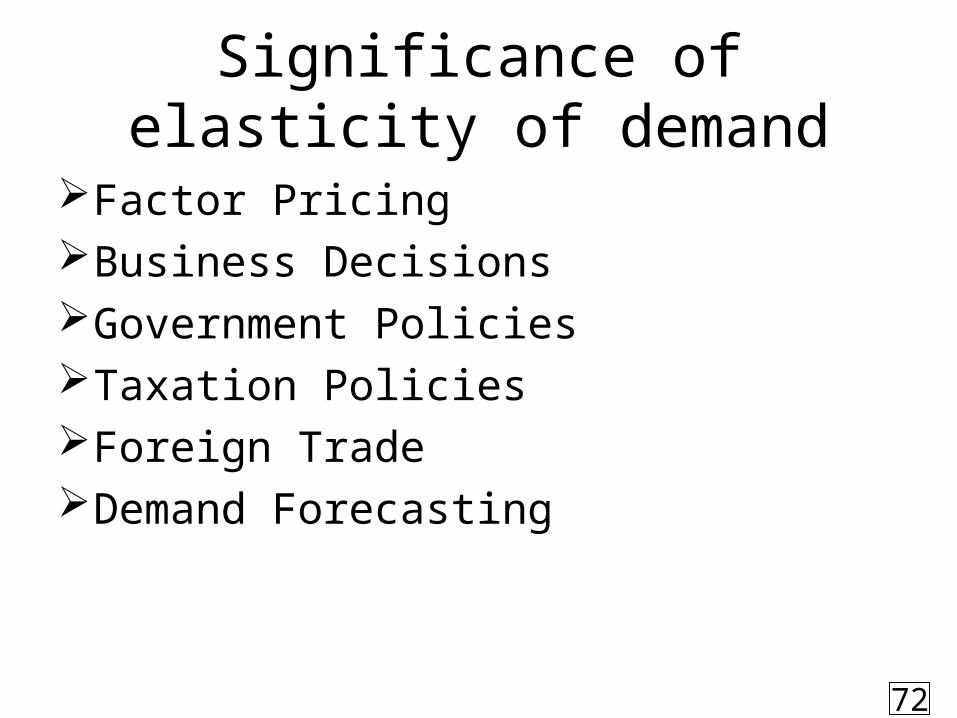
Significance of elasticity of demand
Factor PricingBusiness DecisionsGovernment PoliciesTaxation PoliciesForeign TradeDemand Forecasting
72
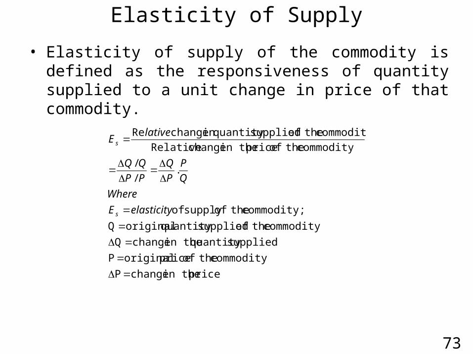
Elasticity of Supply
• Elasticity of supply of the commodity is defined as the responsiveness of quantity supplied to a unit change in price of that commodity.
73
price in the change P
commodity theof price original P
suppliedquantity in the change Q
commodity theof suppliedquantity original Q
commodity; theofsupply of
./
/
commodity theof price in the change Relative
commodity theof suppliedquantity in change Re
elasticityE
Where
Q
P
P
Q
PP
lativeE
s
s
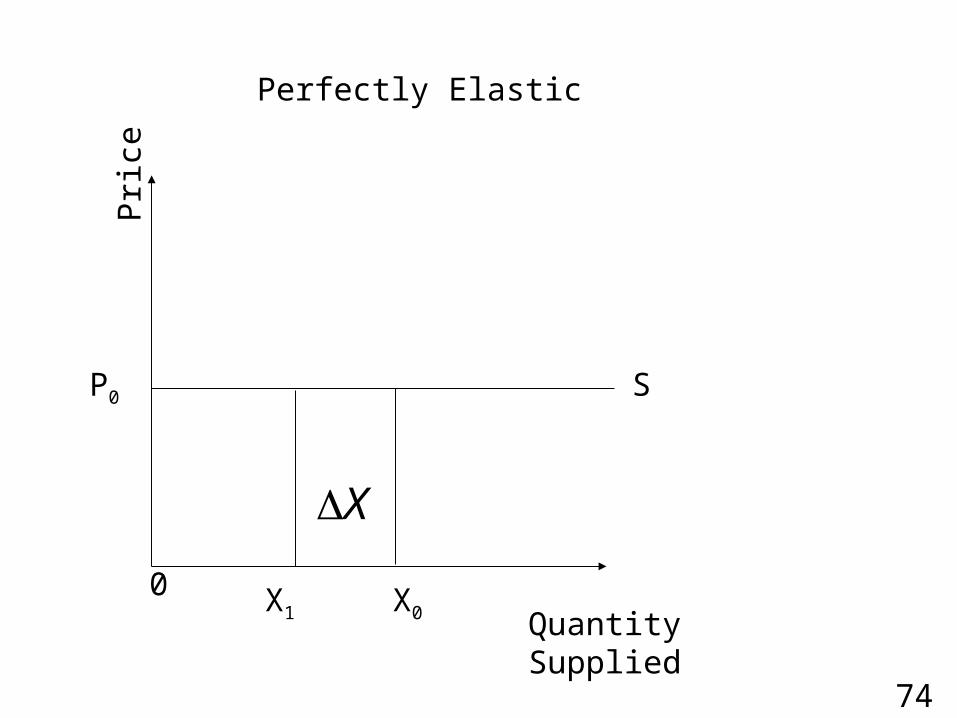
0 X0
S
Quantity Supplied
Pri
ce
X
P0
X1
Perfectly Elastic
74
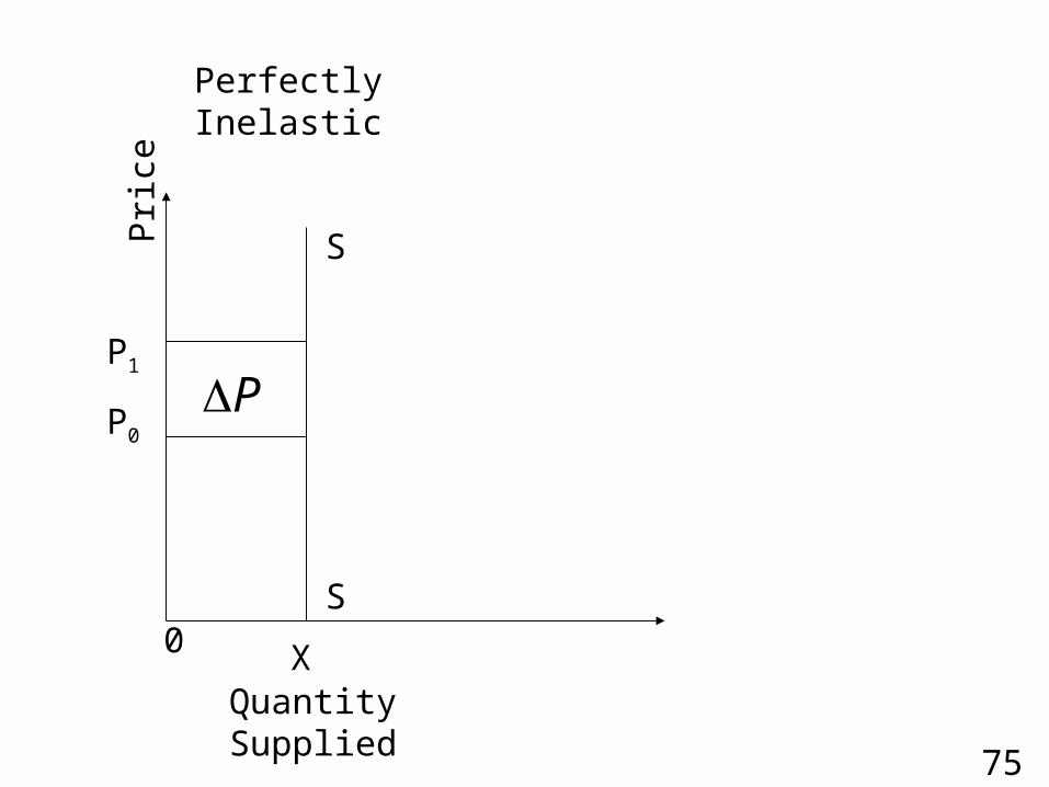
0
S
Quantity Supplied
Pri
ce
PP0
X
P1
S
Perfectly Inelastic
75

0 X0
S
Quantity Supplied
Pri
ce
P1
P0
X1
D
P
X
Relatively Inelastic
76
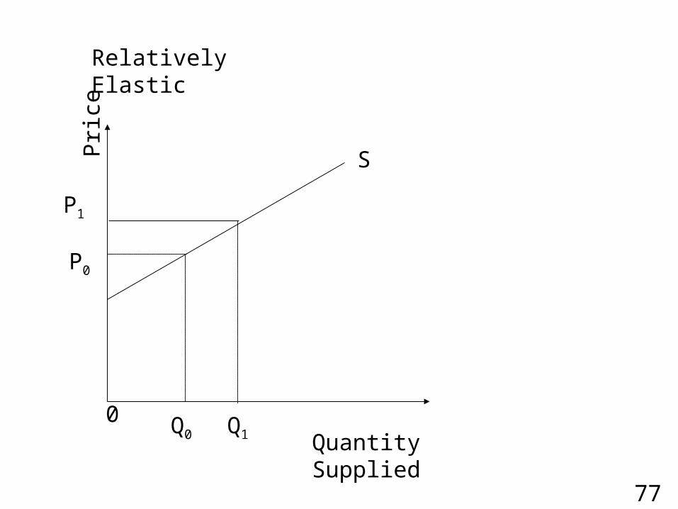
P1
0 Q0 Q1
S
Quantity Supplied
Pri
ce
P0
Relatively Elastic
77
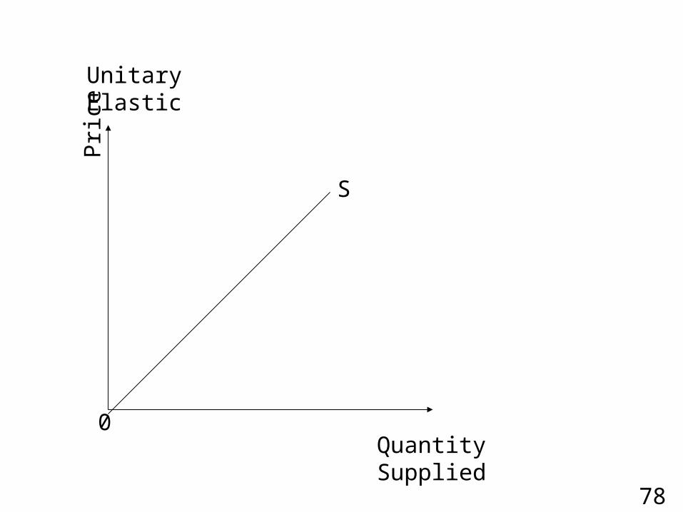
S
0Quantity Supplied
Pri
ceUnitary Elastic
78
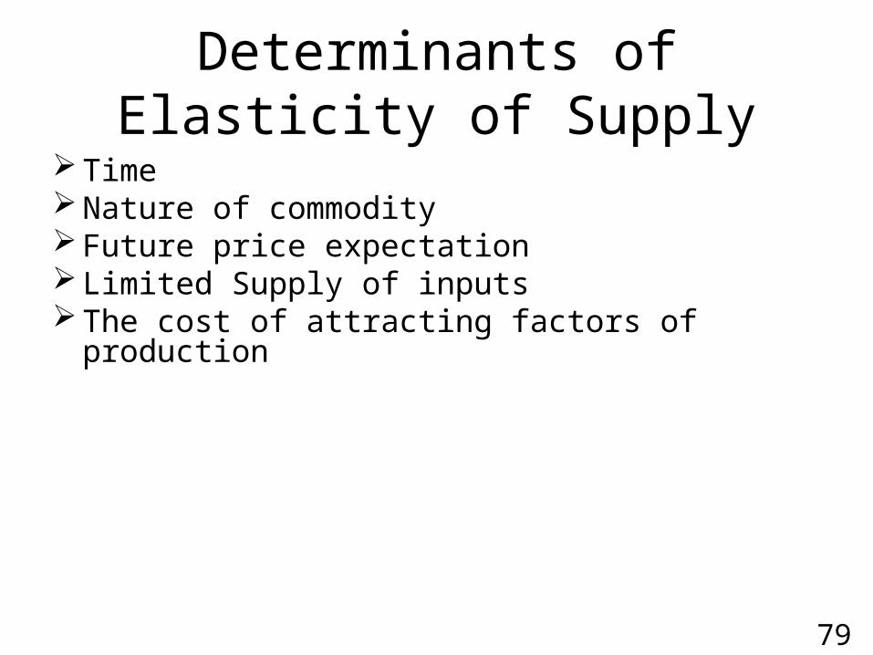
Determinants of Elasticity of Supply
Time Nature of commodity Future price expectation Limited Supply of inputs The cost of attracting factors of production
79