Journal of Geophysical Research: Planets

RESEARCH ARTICLE10.1002/2013JE004459

Key Points:• We present models of the tidal

deformation of Mercury based onMESSENGER results

• Tides are sensitive to size and den-sity of the core and rheology ofouter shell

• The presence of a FeS layer wouldincrease the tidal response

Correspondence to:S. Padovan,sebastiano.padovan@ucla.edu

Citation:Padovan, S., J.-L. Margot, S. A. Hauck II,W. B. Moore, and S. C. Solomon (2014),The tides of Mercury and possibleimplications for its interior structure,J. Geophys. Res. Planets, 119, 850–866,doi:10.1002/2013JE004459.

Received 12 JUN 2013

Accepted 12 MAR 2014

Accepted article online 18 MAR 2014

Published online 21 APR 2014

The tides of Mercury and possible implicationsfor its interior structureSebastiano Padovan1, Jean-Luc Margot1,2, Steven A. Hauck, II3,William B. Moore4,5, and Sean C. Solomon6,7

1Department of Earth, Planetary, and Space Sciences, University of California, Los Angeles, California, USA, 2Departmentof Physics and Astronomy, University of California, Los Angeles, California, USA, 3Department of Earth, Environmental, andPlanetary Sciences, Case Western Reserve University, Cleveland, Ohio, USA, 4Department of Atmospheric and PlanetarySciences, Hampton University, Hampton, Virginia, USA, 5National Institute of Aerospace, Hampton, Virginia, USA,6Lamont-Doherty Earth Observatory, Columbia University, Palisades, New York, USA, 7Department of TerrestrialMagnetism, Carnegie Institution of Washington, Washington, District of Columbia, USA

Abstract The combination of the radio tracking of the MErcury Surface, Space ENvironment,GEochemistry, and Ranging spacecraft and Earth-based radar measurements of the planet’s spin state givesthree fundamental quantities for the determination of the interior structure of Mercury: mean density 𝜌,moment of inertia C, and moment of inertia of the outer solid shell Cm. This work focuses on the additionalinformation that can be gained by a determination of the change in gravitational potential due toplanetary tides, as parameterized by the tidal potential Love number k2. We investigate the tidal responsefor sets of interior models that are compatible with the available constraints (𝜌, C, and Cm). We show that thetidal response correlates with the size of the liquid core and the mean density of material below the outersolid shell and that it is affected by the rheology of the outer solid shell of the planet, which depends onits temperature and mineralogy. For a mantle grain size of 1 cm, we calculate that the tidal k2 of Mercury isin the range 0.45 to 0.52. Some of the current models for the interior structure of Mercury are compatiblewith the existence of a solid FeS layer at the top of the core. Such a layer, if present, would increase the tidalresponse of the planet.

1. Introduction

In the absence of an in situ geophysical network, what we know of the interior of Mercury is based on acombination of Earth-based observations, spacecraft exploration, and theoretical insight. Earth-based radarobservations provide measurements of the obliquity of Mercury and the amplitude of its forced libration[Margot et al., 2007, 2012]. Through radio tracking of the MErcury Surface, Space ENvironment, GEochem-istry, and Ranging (MESSENGER) spacecraft, the gravitational field of the planet has been determined[Smith et al., 2012]. Given that Mercury is in a Cassini state [Colombo, 1966; Peale, 1969], the spin parameters(obliquity 𝜃 and angle of forced libration in longitude 𝛾), when combined with the second harmonic degreecomponents of the gravity field (J2 and C22), provide two important integral constraints for the interior ofMercury: the moment of inertia C [Peale, 1969] and, in the presence of a global liquid layer, the moment ofinertia of the outer solid shell Cm [Peale, 1976]. These two moments, along with the mean density 𝜌, are threeconstraints that any model of the interior of Mercury must satisfy [Hauck et al., 2013].

The measurement of the deformation of a planet due to periodic tidal forcing can be used to place addi-tional bounds on the interior structure, because the tidal response is a function of the density, rigidity, andviscosity of the subsurface materials. This property has been applied in the past to support the hypothesisof a liquid core in Venus [Konopliv and Yoder, 1996] and a global liquid ocean in Titan [Iess et al., 2012]. Yoderet al. [2003] used the measurement of the tides to reveal the liquid state of the Martian core and to estimateits radius. It is interesting to note that the interior structures of Venus and Mars are currently less well charac-terized than that of Mercury, since for Mars the moment of inertia of the outer solid shell is not known, andfor Venus only the mean density and k2 tidal deformation are known, but no moment of inertia informationis available.

The motivation for this paper is to explore the information that can be gained about the interior of Mercuryby the combination of the determinations of 𝜌, C, and Cm with the measurement of k2, which will indicatethe 88 day annual tidal k2.

PADOVAN ET AL. ©2014. American Geophysical Union. All Rights Reserved. 850

Journal of Geophysical Research: Planets 10.1002/2013JE004459

We model the tidal response of Mercury for a range of interior structures that are compatible with themean density 𝜌 and the moments of inertia C and Cm [Hauck et al., 2013]. The formalism that we employ isdescribed in section 2, and section 3 describes the interior models that we use and the assumptions that wemake in the evaluation of the tidal response. The rheology of the outer solid shell is discussed in section 4.The results of our simulations are presented in section 5 (the minor effects of the properties of the inner coreon the tidal response are explored in Appendix A). We discuss the implications of the detection of the tidalresponse for the physical characterization of the interior of Mercury in section 6.

2. Planetary Tidal Deformation

Mercury’s solar tides are caused by the difference in the gravitational attraction of the Sun across the planet.Denoting the mass of the Sun by MS, the expression for the solar tide-generating potential Φ at a point Pinside the planet is

Φ =GMS

d=

GMS

rS

[ ∞∑n = 2

(r′

rS

)n

Pn

(cos𝜓P

)]=

∞∑n = 2

Φn, (1)

where the summation follows from the expansion for (1∕d), and d is the distance between P and the Sun[e.g., Arfken and Weber, 2005]. The angle 𝜓P is the angle between r′ and rS, the distances from the center ofmass of the body to P and to the Sun, respectively. Pn indicates the Legendre polynomial of degree n. G is thegravitational constant. We introduce Φn to highlight the dependence of Φ on the nth power of the factor(r′∕rS) ≪ 1. For a point on the surface, we set r′ = RM, the radius of Mercury, and rS equal to aM, the semi-major axis of Mercury’s orbit, and we can express the largest component of the potential as g𝜁P2(cos𝜓P),where g = (GMM∕R2

M) is the gravitational acceleration at the surface, MM is the mass of Mercury, 𝜁P2(cos𝜓P)is the height of the equilibrium tide [Murray and Dermott, 1999], and

𝜁 =MS

MM

(RM

aM

)3

RM. (2)

Among the terrestrial planets, 𝜁 is the largest for Mercury, with a value of ∼1.10 m (for comparison 𝜁Venus ∼0.43 m, 𝜁Earth ∼ 0.16 m, and 𝜁Mars ∼ 0.03 m).

The harmonic expansion of the tide-generating potential in equation (1) can be used to identify all thedifferent tidal components (in period and amplitude) generated by the Sun at Mercury [Van Hoolst andJacobs, 2003]. The largest component has a timescale equal to the orbital period of Mercury around the Sun(∼ 88 days). This annual tidal perturbation periodically modifies the shape of Mercury and thus the dis-tribution of matter inside the planet, with an accompanying modification of its gravitational field. Thismodification is parameterized with the potential Love number k2, which relates the additional potential 𝜙2t

due to the deformation of the planet to the tide-generating potential Φ2 due to the Sun:

𝜙2t = k2(𝜔) Φ2. (3)

The subscript 2 indicates that the main deformation is generated by the largest term of the expansion,which corresponds to n = 2. The frequency 𝜔 indicates that the response of the body, described by k2,

depends on the period (i.e., frequency) of the applied forcing, which for the case considered here is the 88day period solar tide.

The study of the deformation of a planet under the perturbation of an external potential requires the solu-tion of the equations of motion inside the body. Using a spherical harmonic decomposition in latitude andlongitude, we transform these three second-order ordinary differential equations into six first-order lineardifferential equations in radius [Alterman et al., 1959]. The motion is controlled both by material stresses(elastic or viscoelastic) and gravitational forces, the latter originating from a gravitational potential that is thesum of the self-gravitation of the planet and the external tidal potential. The framework for the solution isformally the same both for elastic rheologies and for viscoelastic rheologies, thanks to the correspondenceprinciple [Biot, 1954]. The results presented in the following sections are obtained by modeling Mercury as

PADOVAN ET AL. ©2014. American Geophysical Union. All Rights Reserved. 851

Journal of Geophysical Research: Planets 10.1002/2013JE004459

a series of homogeneous incompressible layers. Each layer is characterized by thickness, density, rigidity,and viscosity [Wolf, 1994]. In evaluating the tidal response, we use the formalism developed by Moore andSchubert [2000].

The possible values for the k2 of a planet range between 0 for a perfectly rigid body that does not deform,and 1.5, the value for a homogeneous fluid body (for these idealized bodies the limits are independent ofthe forcing frequency). Values for k2 have been determined for Venus [Konopliv and Yoder, 1996], the Moon[Konopliv et al., 2013; Lemoine et al., 2013], Mars [Konopliv et al., 2011], and Titan [Iess et al., 2012]. The k2 ofthe Moon is uncertain at the ∼ 0.5% level, a result of the high-quality data obtained with the Gravity Recov-ery and Interior Laboratory mission [Zuber et al., 2013]. For Mars the estimate is uncertain at the ∼ 5% level,a result obtained by combining data from a large number of spacecraft missions, including a lander and twoyears of tracking data from the low-altitude, nearly circular orbital phase of the Mars Reconnaissance Orbiter.For Venus and Titan the estimates have an uncertainty ≳ 10%. A numerical simulation of the determina-tion of Mercury’s k2 with BepiColombo, the future dual orbiter mission to Mercury by the European SpaceAgency and the Japan Aerospace Exploration Agency, indicates an expected accuracy of ∼ 1% [Milani et al.,2001]. This figure represents a lower bound for MESSENGER, because its eccentric orbit makes the detec-tion of k2 more challenging. The uncertainty on the determination of the k2 of Mercury as obtained fromMESSENGER is expected to be ∼ 10% [Mazarico et al., 2014].

The mantle of Earth responds elastically on the short timescales associated with the waves generated byearthquakes but flows like a fluid on the geologically long timescales of mantle convection. The Maxwellrheological model is the simplest model that captures this short- and long-timescale behavior. It is com-pletely defined by two parameters: the unrelaxed (infinite-frequency) rigidity 𝜇U and the dynamic viscosity𝜈. The Maxwell time, defined as

𝜏M = 𝜈

𝜇U, (4)

is a timescale that separates the elastic regime (forcing period ≪ 𝜏M) from the fluid regime (forcing period≫ 𝜏M). This simple rheological model is sufficiently accurate for the crust, which is cold and responds elasti-cally, and the liquid core, which has zero rigidity and therefore a fluid response. The inner core, if present, hasa negligible effect on the tidal response (Appendix A), so for simplicity we use a Maxwell model to describeits rheology. Nevertheless, the Maxwell model does not provide a good fit to laboratory and field data in thelow-frequency seismological range, and thus it should not be used to model the response of the mantle attidal frequencies [e.g., Efroimsky and Lainey, 2007; Nimmo et al., 2012].

Jackson et al. [2010] explored three different parameterizations (Burgers, extended Burgers, and Andradepseudoperiod) to fit torsional oscillation data from a set of melt-free olivine samples. Both the Burgers mod-els and the Andrade model provide a good fit for the low-frequency data. The small number of parametersrequired for the Andrade model makes it more attractive to model the rheology of Mercury, for which welack any ground-truth data. Note, however, that both the Burgers models and the Andrade model havenot been tested at periods longer than 103 s, so when applied to the study of planetary tidal deformation(period > 106 s), they both need to be extrapolated (for an application of the extended Burgers model tothe mantle of the Moon and Mars, see Nimmo et al. [2012] and Nimmo and Faul [2013], respectively).

We report here the expressions for the real and imaginary part of the dynamic compliance J(𝜔) for theAndrade-pseudoperiod model, as described by Jackson et al. [2010]:

JR(𝜔) =1𝜇U

{1 + 𝛽∗Γ(1 + n)𝜔−n cos

(nπ2

)}, (5)

JI(𝜔) =1𝜇U

{𝛽∗Γ(1 + n)𝜔−n sin

(nπ2

)+ 1𝜔𝜏M

}(6)

The unrelaxed rigidity is 𝜇U and 𝛽∗ =𝛽𝜇U. The coefficient 𝛽 , along with n, appears in the expression ofthe Andrade creep J(t)=1∕𝜇U +𝛽tn + t∕𝜈, where Γ is the gamma function and 𝜏M the Maxwell time. The

PADOVAN ET AL. ©2014. American Geophysical Union. All Rights Reserved. 852

Journal of Geophysical Research: Planets 10.1002/2013JE004459

Table 1. Rheological Models for the Interior of Mercurya

Layer Model Parameter Definition Value Notes

Crust Maxwell section 4.3𝜇U Unrelaxed rigidity 55 GPa𝜈 Dynamic viscosity 1023 Pa s

Mantle Andradeb section 2𝜇U Unrelaxed rigidity 59–71 GPa section 4.2Tb Mantle basal temperaturec 1600–1850 K section 3.2n Andrade creep coefficient 0.3𝛽∗ Andrade creep parameter 0.02PR Reference pressure 0.2 GPaTR Reference temperature 1173 KdR Reference grain-size 3.1 μmd Grain size 1 mm–1 cmm Grain size exponent 1.31V Activation volume 10−5 m3 mol−1

EB Activation energy 303 × 103 kJ mol−1

FeS Andraded section 4.4Outer core Maxwell section 2

𝜇U Unrelaxed rigidity 0 Gpa𝜈 Dynamic viscosity 0 Pa s

Inner core Maxwell Appendix A𝜇U Unrelaxed rigidity 1011 Pa𝜈 Dynamic viscosity 1020 Pa s

aThe models are introduced in section 2.bThe fixed parameters of the Andrade model are based on the results of Jackson et al. [2010].cHere we report Tb because the temperature T in equation (7) depends on the temperature profile,

which is controlled by Tb.dThe FeS layer is assumed to have the same rheology as that of the base of the mantle.

frequency 𝜔 is obtained from 𝜔 = 2π∕XB, where XB is the pseudoperiod master variable introduced byJackson et al. [2010]:

XB = T0

(d

dR

)−m

exp[(

−EB

R

)(1T− 1

TR

)]exp

[(−VR

)(PT−

PR

TR

)], (7)

which takes into account the effects of pressure P, temperature T , and grain size d. The subscript R indi-cates reference value. T0 is the forcing period (for Mercury ∼ 88 days). The exponent m characterizes thedependence on the grain size, which in principle can be different for anelastic processes (ma) and for viscousrelaxation (mv). We tested that at the frequency of the Mercury tide, the effect is minor, and we assumedma = mv = m. The other quantities are defined in Table 1. The dynamic compliance was evaluated by set-ting the value of 𝜏M in equation (6) equal to the reference value (𝜏MR = 105.3 s) reported by [Jackson et al.,2010] and including the effects of T , P, and d through the pseudoperiod master variable defined in equation(7). The dynamic compliance is related to the inverse quality factor Q−1 and the rigidity 𝜇 by

Q−1(𝜔) =JI(𝜔)JR(𝜔)

, (8)

𝜇(𝜔) =[

J2R(𝜔) + J2

I (𝜔)]−1∕2

. (9)

To illustrate the importance of choosing a realistic rheological model, in Figure 1 we show how the rigidityof a material with 𝜇U = 65 GPa varies as a function of the forcing frequency for two temperatures, at a pres-sure of 5.5 GPa, representative of conditions at the base of the mantle of Mercury [Hauck et al., 2013]. Boththe Maxwell rheological model and the Andrade model are plotted. They both predict a fluid response (i.e.,zero rigidity) at high temperatures and/or long forcing frequencies, but the Maxwell model underestimatesnonelastic effects at forcing periods that are shorter than the Maxwell time. This effect is particularly rele-vant for Mercury, for which the core-mantle boundary temperature may be above 1600 K [Rivoldini and VanHoolst, 2013; Tosi et al., 2013].

PADOVAN ET AL. ©2014. American Geophysical Union. All Rights Reserved. 853

Journal of Geophysical Research: Planets 10.1002/2013JE004459

Figure 1. Comparison of the Andrade (solid lines) and Maxwell(dashed lines) rheological models at a pressure of 5.5 GPa for twodifferent temperatures: T = 1400 K (red) and T = 1800 K (green).The solid colored vertical lines represent the Maxwell times. Thedash-dotted line indicates the forcing frequency of Mercury’s tide.Note that at T = 1800 K the Maxwell model overestimates the rigid-ity at the tidal frequency by about 35% compared with the Andrademodel. The unrelaxed modulus used in these example is 65 GPa.

3. Methods

Throughout this work (except section 3.1),we use models compatible with the avail-able constraints, i.e., mean density 𝜌,moment of inertia C, and moment of iner-tia of the solid outer shell Cm (section 1).By compatible we mean that the distribu-tions of 𝜌, C, and Cm in the set of interiormodels considered here are approxi-mately Gaussian with means and standarddeviations that match the nominal valuesof the observables and their 1 standarddeviation errors. The mean density 𝜌 hasa Gaussian distribution with mean andstandard deviation equal to 5430 kg/m3

and 10 kg/m3, respectively. For C andCm, we choose Gaussian distributionswith means and standard deviationsdefined by the observed values and errorsreported by Margot et al. [2012]. Accord-ingly, C∕MMR2

M = 0.346 ± 0.014 andCm∕C = 0.431±0.025 [Margot et al., 2012].

The small abundance of Fe and relatively large abundance of S at the surface of Mercury imply stronglyreducing conditions within the planet [Nittler et al., 2011]. Under these conditions both silicon and sulfurlikely partitioned into the core during Mercury’s formation and differentiation [Hauck et al., 2013]. Of thefive compositional models for the interior of Mercury analyzed by Hauck et al. [2013], we focus on two setsthat have a Si-bearing core, because they are consistent with the inferred reducing conditions. The majordifference between the two sets is the presence or absence of a solid FeS layer at the top of the core. Welabel these two sets the FeS set and NoFeS set, respectively.

The possible presence of an FeS layer was initially predicated on the basis of the inferred highly reducingconditions and the then-best estimate of the high mean density of the outer solid shell [Smith et al., 2012].Improved values of the obliquity 𝜃 [Margot et al., 2012] led to a revised value for the mean density of theouter solid shell [Hauck et al., 2013] and made the density argument for the presence of the FeS layerless compelling. Nevertheless, the geochemical argument supporting the presence of the FeS layer is stillvalid [Hauck et al., 2013], and a conductive layer above the convective liquid core is one of the possibleexplanations for Mercury’s weak magnetic field [Christensen, 2006; Anderson et al., 2012].

3.1. Radial Density ProfileThe radial density profiles that we used as input [Hauck et al., 2013] are given as series of constant-propertylayers, going from the center to the surface. The crust, mantle, and FeS layer are modeled asconstant-density shells. This simplification is justified by the small thickness of the outer solid shell ofMercury and by the relatively low surface gravitational acceleration, but does not affect the characterizationof the interior of the planet on the basis of the measured values of 𝜌, C, and Cm [Hauck et al., 2013]. The core(inner + outer) is represented with ∼1000 layers in order to take into account the effects of self-compressionand temperature in the equation of state for core materials, as was done by Hauck et al. [2013]. However, theLove number k2 is a global parameter, summarizing the response of the planet to tidal forcing, and it is notvery sensitive to the fine density structure. We verified that k2 calculations can be performed accurately withsimplified, 4- or 5-layer models instead of the original ∼ 1000-layer models. In order to establish this point,we used a random sample of 100 models drawn from the FeS set and constrained only by the mean density𝜌 of Mercury. For this test we did not apply the moment of inertia constraints (C and Cm), as this allowed usto explore a larger parameter space and resulted in a more robust test. For each one of the 100 models wecomputed an averaged version, characterized by five constant-density layers. Computed k2 values for the

PADOVAN ET AL. ©2014. American Geophysical Union. All Rights Reserved. 854

Journal of Geophysical Research: Planets 10.1002/2013JE004459

0.980.991.001.01

0 20 40 60 80 100

0.2

0.3

0.4

0.5

0.6

0.7

Figure 2. Effect of the radial density profile on the magnitude of k2. (top)For each of a set of 100 models, the value of k2 has been calculated bothfor the ∼1000 layer version (k2(M)) and for the five-layer version (k2(Av)).(bottom) The ratio of the two determinations, which in most cases iswithin 2% of unity. The models used for this plot are constrained only bythe mean density of Mercury.

∼1000 layer models and the corre-sponding 5-layer models are shownin Figure 2 (top). Their ratio (Figure 2,bottom) indicates that errors intro-duced by using the simplified modelsare ≲ 2%. In view of this result and ofthe ∼10% accuracy of MESSENGER’s k2

determination (section 2), in what fol-lows we show results obtained withthe simplified 4- or 5-layer models. Thisapproach reduces the computationalcost by ∼3 orders of magnitude.

3.2. Pressure and TemperatureProfiles in the MantleTo calculate a rheological profilefor the mantle of Mercury with theAndrade rheological model describedin section 2, the pressure and tem-perature as a function of depth mustbe calculated.

At the radius r in the mantle the pressure is simply obtained as an overburden load P(r) = g[𝜌chc + 𝜌mhm(r)],where the subscripts “c” and “m” refer to the crust and mantle, respectively. The crustal thickness is hc, andhm(r) is the thickness of the mantle above r (i.e., r + hm(r) + hc = RM).

We obtained the temperature profile by solving the static heat conduction equation with heat sources inspherical coordinates [e.g., Turcotte and Schubert, 2002] in the mantle and crust:

k1r2

ddr

(r2 dT

dr

)+ 𝜌H = 0. (10)

In equation (10) k is the thermal conductivity, 𝜌 is the density, and H is the heat production rate.

We assumed a homogeneous distribution of heat sources in the crust and in the mantle. The distribution inthe crust might be exponential as in the crust of the Earth, but we verified that this would only marginallyaffect the deep mantle temperature profile. The value of H at the surface, H0, has been inferred from MES-SENGER measurements and is equal to H0 = 2.2 × 10−11 W kg−1 [Peplowski et al., 2011]. We adopted thesurface value H0 for the heat production rate in the crust, Hc =H0. For the distribution of heat sources in themantle we used Hm =H0 ∕2.5, which is compatible with the enrichment factor derived by Tosi et al. [2013].The value of k is set to 3.3 W m−1 K−1.

As boundary conditions, we applied the surface temperature TS and the temperature at the base of the man-tle Tb. TS is set to 440 K, a value obtained with a simple equilibrium temperature calculation. Therefore, inour models the temperature profile is controlled by the temperature Tb. There are currently few constraintson Tb, but two independent sets of workers [Rivoldini and Van Hoolst, 2013; Tosi et al., 2013] point to therange 1600–1900 K. We defined two end-member profiles: a cold mantle with Tb = 1600 K and a hot man-tle with Tb = 1850 K. We consider Tb = 1850 K as our hot mantle case, since, from the peridotite solidus ofHirschmann [2000], Tb = 1900 K would result in partial melting at the base of the mantle (Figure 3). We didnot consider in this work the presence of partial melting.

The rheological models described in section 2 strongly depend on the temperature. Our end-member tem-perature profiles are obtained under the assumption of a conductive mantle. This assumption is consistentwith the results of Tosi et al. [2013], which indicate that the mantle of Mercury is most likely conductive atthe present time. Nevertheless, a present-day convective mantle is not excluded [Michel et al., 2013; Tosiet al., 2013]. A convective mantle for the Tb =1850 K case would result in partial melting (Figure 3). A con-vective profile with Tb =1600 K would be more dissipative and deformable than the conductive case (sincein the convective envelope the temperature is approximately constant and equal to Tb), but this effect is

PADOVAN ET AL. ©2014. American Geophysical Union. All Rights Reserved. 855

Journal of Geophysical Research: Planets 10.1002/2013JE004459

Figure 3. Temperature (solid line) as a function of depth for a model witha 2020 km radius core and a 50 km thick crust. The values for the heat pro-duction rate in the crust and mantle are indicated. The dots represent themidpoint of each mantle sublayer, for which the temperature and pressureare used to derive a rheology for the sublayer. The peridotite solidus ofHirschmann [2000] is also shown.

similar to a conductive case with ahigher Tb. Our two end-member tem-perature profiles thus capture thepossible effects of temperature varia-tions in the mantle of Mercury, underthe assumption that there is no partialmelting in the mantle.

To model the rheology of the man-tle as a function of depth, we dividedit into sublayers. Starting from thecore-mantle boundary, we dividedthe mantle in 40 km thick sublayers,as illustrated in Figure 3. For eachsublayer the pressure and the temper-ature at the midpoint were calculated.The complex compliance for eachsublayer was obtained with equations(5) and (6) of section 2. The rigiditywas calculated with equation (9). Theviscosity is then given by the expres-sion 𝜈 = 1∕(JI𝜔). It is the viscosity of

a Maxwell model with the same complex compliance, i.e., with the same rheology. The value of rigidity andviscosity so calculated were taken as representative of the full sublayer.

The Andrade rheological model has been successfully applied to the description of dissipation in rocks,ices, and metals [i.e., Efroimsky, 2012, and references therein]. The model described in section 2 currentlyrepresents the best available Andrade model parameterization that incorporates the effects of temperature,pressure, and grain size on the rheology. However, the parameters that are kept fixed in the model (listedin Table 1) are based on laboratory data on olivine [Jackson et al., 2010]. In what follows we apply theAndrade model of section 2 to different mineralogical models for the mantle of Mercury. We thus assumethat the fixed parameters of olivine can be applied to other minerals. This assumption is not strictly correct,especially for mantle models in which olivine is not the dominant phase, but the broad applicability of theAndrade model to describe materials as chemically and physically different as ices and silicates indicatesthat the model we use should provide a good description of the rheology of silicate minerals.

4. Assessment of the Rheology of the Outer Solid Shell

The unrelaxed rigidity is a parameter required to characterize the rheology and thus the response to thetidal forcing. Different minerals have different rigidity values, so the mineral assemblages of the mantle andcrust determine their rigidities. In this section we assess the impact of the composition on the rigidity ofthe mantle and the crust. Table 2 contains data for minerals that are used below in modeling the rigidity ofthe mantle and crust of Mercury. In addition, we describe our assumptions in modeling the response of theFeS layer.

4.1. Mineralogical Models for the MantleFor the mineralogy of the mantle, we use the works of Rivoldini et al. [2009] and Malavergne et al. [2010]as references. Malavergne et al. [2010] calculated the expected mineralogy of the mantle of Mercury as afunction of pressure, given two different assumed bulk compositions for the whole planet, an enstatitechondrite (EH) and a Bencubbin-like chondrite (CB). The EH chondrite provides a good compositional andmineralogical match to the data of the X-Ray Spectrometer (XRS) on MESSENGER [Weider et al., 2012], whichare compatible with the data from the Gamma-Ray Spectrometer (GRS) [Evans et al., 2012]. The XRS and theGRS are sensitive to the top tens of micrometers and centimeters of near-surface material, respectively, andthe consistency between the results of the two instruments indicates that the top tens of centimeters ofMercury’s regolith are vertically homogeneous [Evans et al., 2012]. Despite the apparent good agreementbetween XRS and GRS results and enstatite chondrite compositions, the metal fraction in EH chondrites is

PADOVAN ET AL. ©2014. American Geophysical Union. All Rights Reserved. 856

Journal of Geophysical Research: Planets 10.1002/2013JE004459

Table 2. Minerals Relevant to the Mantle and Crust of Mercurya

Abbr. 𝜌0 𝜇0 𝜇′R|||0 𝜇′T

|||0(kg/m3) (GPa) (GPa/K)

Garnet Grt 3565 + 760𝜒Fe 92 + 7𝜒Fe 1.4 −0.010Orthopyroxene Opx 3194 + 799𝜒Fe 78 + 10𝜒Fe 1.6 −0.012Clinopyroxene Cpx 3277 + 380𝜒Fe 67 − 6 𝜒Fe 1.7 −0.010Quartz Qtz 2650 44.5 0.4 −0.001Spinel Spl 3580 + 700𝜒Fe 108 − 24 𝜒Fe 0.5 −0.009Plagioclase Pl 2750 40.4 2.5 −0.002Merwinite Mw 3330 81 1.4 −0.014Olivine Ol 3222 + 1182𝜒Fe 81 − 31 𝜒Fe 1.4 −0.014

aAbbr. denotes mineral abbreviation [Siivola and Schmid, 2007]. A subscript“0” indicates standard ambient temperature and pressure (298 K, 105 Pa); densityis 𝜌; 𝜇, 𝜇′

P, and 𝜇′T are the rigidity and its pressure and temperature deriva-

tives, respectively; and 𝜒Fe is the mole fraction of iron. Data in this table aretaken from the compilations of Sobolev and Babeyko [1994], Vacher et al. [1998],Cammarano et al. [2003], Verhoeven et al. [2005], and Rivoldini et al. [2009].

lower than the bulk value for Mercury. The CB chondrites analyzed by Malavergne et al. [2010] have a highermetallic component and thus might represent another possible building block for Mercury. Rivoldini et al.[2009] calculated the expected mineralogy for a set of five models of the mantle of Mercury. These includedthe following: an enstatite chondrite model (EC), similar to the EH case of Malavergne et al. [2010]; a modelin which the building blocks for Mercury are matched compositionally by the chondrules of two metal-richchondrites (MC) [Taylor and Scott, 2005]; a model based on fractionation processes in the solar nebula (MA)[Morgan and Anders, 1980]; the refractory-volatile model (TS) of Taylor and Scott [2005]; and the evaporationmodel of Fegley and Cameron [1987]. The latter is not consistent with the high abundance of sulfur, potas-sium, and sodium in Mercury’s surface materials [Nittler et al., 2011; Peplowski et al., 2011; Evans et al., 2012].We used the composition of these six models to estimate a range for the rigidity of the mantle of Mercury.The mineralogical composition of these models is listed in Table 3.

4.2. Rigidity of the MantleMESSENGER confirmed that the surface of Mercury has an extremely low iron abundance [Nittler et al., 2011;Evans et al., 2012] and showed that a substantial fraction of the surface is volcanic in origin [Denevi et al.,2013]. The low surface abundance of FeO is an indication that the source regions of volcanic material arealso FeO poor, since FeO does not undergo major fractionation during partial melting [Taylor and Scott,2005]. However, under the highly reducing conditions inferred for Mercury, part of the iron in the silicateshell is present as sulfides and metal [Zolotov et al., 2013]. In calculating the rigidity of the mantle, we assumethat the silicate minerals contain no iron. In other words, we assume that 𝜒Fe = 0 in Table 2. The effects ofsmall amounts of iron-rich minerals are small compared with the uncertainties introduced by the unknownmineralogy of the mantle of Mercury. It should be noted, however, that at least for olivine the rheological

Table 3. Models for the Mantle of Mercurya

Model Grt Opx Cpx Qtz Spl Pl Mw Ol 𝜇c (GPa)CB - 66 4 22 4 4 - - 59EH - 78 2 8 - 12 - - 65MA 23 32 15 - - - - 30 69TS 25 - - - 8 - 2 65 71MC 15 50 9 - - - - 26 68EC 1 75 7 17 - - - - 60

aTwo capital letters identify the model (details in section 4.1). CB and EH: Malavergneet al. [2010], MA: Morgan and Anders [1980], TS and MC: Taylor and Scott [2005], and EC:Wasson [1988]. The central part of the table gives the mineralogical content in terms of thevol % of its components [after Malavergne et al., 2010; Rivoldini et al., 2009]. Mineral abbre-viations are defined in Table 2. A dash indicates that the mineral is absent. The compositerigidity 𝜇c is evaluated as the Hill rigidity at T = 1173 K and P = 0.2 GPa.

PADOVAN ET AL. ©2014. American Geophysical Union. All Rights Reserved. 857

Journal of Geophysical Research: Planets 10.1002/2013JE004459

Table 4. Composition and Rigidity of the Crust ofMercurya

Model Ol Opx Pl Spl Qz 𝜇c (GPa)

SP 2 44 26 6 22 53 − 58SPNa 8 30 57 5 - 51 − 53IcP-HCT 2 59 29 1 9 57 − 60

a“Model” column: SP stands for smooth plainsand IcP-HCT stands for intercrater plains and heavilycratered terrain. SPNa takes into account the differ-ence that might arise with a different Na abundance[see Stockstill-Cahill et al., 2012]. The central partof the table gives the mineralogical compositionin weight percent. In the last column the compos-ite rigidity is calculated with Hill’s expression. Therange in 𝜇c for each model is given by the differentamounts of end-members (i.e., forsterite and fayalitein the olivine solid-solution series).

properties show a strong dependence on the ironcontent [Zhao et al., 2009].

For each mineralogical model of the mantle in Table 3,we calculate the composite rigidity at the referenceconditions of TR = 1173 K and PR = 0.2 GPa, requiredfor the Andrade model (equation (7)). First, for eachmineral the rigidity at TR and PR is obtained from theparameters in Table 2 with the expression

𝜇U(TR, PR) =[𝜇0 + (T − TR)

d𝜇dT

+ (P − PR)d𝜇dP

]. (11)

The composite rigidity is obtained with Hill’s expres-sion, which is an average between the Reuss and theVoigt rigidities [Watt et al., 1976]. Table 3 lists the com-posite rigidities so derived for the mantle models. Therange is 59–71 GPa.

4.3. Rigidity and Viscosity of the CrustThe surface of Mercury presents a compositional and morphological dichotomy between the youngersmooth plains (SP) and the older intercrater plains and heavily cratered terrain (IcP-HCT) [Peplowski et al.,2011; Weider et al., 2012]. The majority of the SP, which cover ∼ 27% of the surface of Mercury, is volcanicin origin [Denevi et al., 2013]. From the surface compositional data returned by MESSENGER, Stockstill-Cahillet al. [2012] modeled the expected mineralogy of the IcP-HCT and the northern volcanic plains (NVP). TheNVP is a large contiguous area of volcanic smooth plains [Head et al., 2011] that shows similar compositionto other smooth plains (i.e., Caloris basin interior) [Weider et al., 2012]. Therefore, the mineralogy of the NVPcan be taken as representative of other smooth plains areas. The results of Stockstill-Cahill et al. [2012] aresummarized in Table 4. The table also includes the mineralogy for smooth plains when the effect of uncer-tainties in the Na abundance are taken into account (SPNa). These three mineralogies are used to estimatethe rigidity of the crust of Mercury.

Variations in the temperature and pressure of the crust with depth have negligible effects on the rigidities ofthe individual minerals. Therefore, the composite rigidity is obtained with Hill’s expression using 𝜇0 (Table 2)as the rigidity for each mineral.

The range in crustal rigidity is 51–60 GPa and will likely encompass the actual rigidity of the crust if theIcP-HCT represents the older crust and the SP are representative of the younger crust produced by the mostrecent widespread episodes of partial melting of the mantle. We use the central value of 55 GPa as the rigid-ity of the crust. Its viscosity is set at 1023 Pa s. This choice is not critical since the crust is cold and respondselastically at the forcing frequency of the tide.

4.4. Rheology of the FeS LayerThe procedure used to calculate the rigidity of the mantle minerals cannot be used for the FeS layer becauseof a lack of laboratory data. At the relevant pressures and temperatures of the outer core of Mercury, the FeSwould be in the FeS V phase [Fei et al., 1995]. For FeS V the bulk modulus and its pressure and temperaturederivatives have been measured [Urakawa et al., 2004]. There is no rigidity determination, however. Eventhe rigidity of troilite (or FeS I, the phase at standard pressure and temperature) has never been measured[Hofmeister and Mao, 2003]. Nevertheless, an argument illustrated by Hofmeister and Mao [2003, Figure 7]sets 𝜇FeS I =31.5 GPa. From the phase diagram of FeS [Fei et al., 1995], the conditions at the base of themantle (P ∼5.5 GPa) are close to the melting curve for FeS V. The corresponding homologous temperatureTH, the ratio of the temperature of the material to the solidus temperature, is TH > 0.85. It is often assumedthat the viscosity is proportional to the exponential of the inverse of the homologous temperature [e.g.,Borch and Green, 1987]. Therefore, the viscosity of the FeS layer at the top of the core would be close to thelow viscosity of the melt. These considerations indicate that the FeS layer, if present, is weak.

We consider the effects of the FeS layer only in the cold mantle case (Tb = 1600 K), since for higher tem-peratures the FeS would be liquid (see the phase diagram in Fei et al. [1995]). We assume that the FeS willhave the same rheological properties as the base of the mantle. This assumption is conservative because at

PADOVAN ET AL. ©2014. American Geophysical Union. All Rights Reserved. 858

Journal of Geophysical Research: Planets 10.1002/2013JE004459

Figure 4. The value of k2 as a function of the radius of the liquid core for the NoFeS set. For these data the temperatureat the base of the core is Tb = 1725 K, and the mantle unrelaxed rigidity is 𝜇U = 65 GPa. (left) Colors indicate the meandensity of material below the outer solid shell (OSS). The arrows indicate how the data points would shift with a changein the rheological properties of the OSS. (right) Same as for left panel, but here colors indicate the mean density ofthe OSS.

T = 1600 K, the TH of FeS is larger than TH of the silicates, and from the value of 𝜇FeS I, the unrelaxed rigidityof FeS V is likely to be smaller than that for the silicates.

5. Results: Tidal Response and Interior Properties

The results illustrated below show that models of Mercury with a liquid outer core have k2 ≳ 0.3. For a com-pletely solid model of Mercury (i.e., a model devoid of a liquid outer core), the value of k2 would be reducedby approximately an order of magnitude. Given this variation in the magnitude of k2 between a completelysolid interior and one with a liquid (outer) core, a measurement of the tidal response would provide a con-firmation of the presence of a liquid (outer) core. Its existence has already been inferred from Earth-basedradar measurements [Margot et al., 2007] and also from the interpretation of the magnetic field detected bythe MESSENGER Magnetometer [Anderson et al., 2012]. Therefore, the results presented below focus on themodels of Mercury with a liquid (outer) core that have been described in section 3.

5.1. The Main Parameters Controlling the Tidal DeformationThe tidal response of Mercury is largely controlled by the strength and thickness of the outer solid shell(OSS), much like the similar case for Europa’s ice shell [Moore and Schubert, 2000]. This result is a conse-quence of the presence of a liquid (outer) core, which decouples the shell from the deformation of thedeeper interior. Due to the combined mass and moments of inertia constraints, the thickness of the OSSdepends on the density of the core. This outcome is shown in Figure 4 (left), where the trade-off betweencore density and liquid core radius (i.e., OSS thickness) is seen in the color scale that strongly correlates bothwith the radius of the liquid core and k2. For these models, 𝜇U = 65 GPa, and Tb = 1725 K. A modificationof the rheological properties of the OSS, through a variation of the temperature at the base of the mantleTb and/or of the unrelaxed rigidity 𝜇U, would modify the response as indicated by the arrows in the figure.Note, however, that there is only a weak dependence on the density of the OSS itself, as seen in Figure 4(right), where the colors show the density of the OSS and span nearly the entire range of the response. Thesmall effects of a solid inner core on the tidal response are discussed in Appendix A.

The same set of models used in Figure 4 are shown in Figure 5 in the form of a plot showing how the com-patible models (section 3) are distributed. The availability for Mercury of the three constraints 𝜌, C, and Cm

results in a distribution of the data that is relatively narrow, which makes the determination of k2 in principlevery useful. It has the potential for improving the determination of the location of the radius of the outerliquid core and the mean density of the material below the outer solid shell and of providing insights intothe rheological properties (temperature and rigidity) of the outer solid shell. This improved knowledgewill depend both on the precision of the k2 determination and on the effects of the uncertainties in thetemperature and rigidity of the outer solid shell.

PADOVAN ET AL. ©2014. American Geophysical Union. All Rights Reserved. 859

Journal of Geophysical Research: Planets 10.1002/2013JE004459

Figure 5. Same data as in Figure 4, here plotted using the normalizedpopulation based on the C and Cm determinations.

5.2. Effects of the Mantle Rheologyon the Tidal ResponseIn our models the rheology of theouter shell is controlled by the tem-perature at the base of the mantle Tb

and the unrelaxed rigidity of the man-tle 𝜇U. Figure 6 illustrates the effectson the tidal response of a variation inTb between 1600 K and 1850 K. Forthis case we assumed an unrelaxedmantle rigidity of 𝜇U = 65 GPa. Asexpected, on the basis of the influ-ence of temperature on rheology(Figure 1), a higher Tb correspondsto a weaker outer solid shell, whichin turn has a larger tidal response.In terms of the central values of themodel populations, k2 varies in therange 0.47–0.50.

Basal mantle temperature and unrelaxed rigidity have similar, if opposite, effects on the tidal response,which is enhanced by a higher Tb and/or lower 𝜇U and is diminished by a lower Tb and/or higher 𝜇U. There-fore, there is a trade-off between these two parameters. The full range of tidal responses for the NoFeSmodels is illustrated in Figure 7. The variation in k2 is in the range 0.45–0.52, the former value correspond-ing to the stiff mantle (Tb = 1600 K and 𝜇U = 71 GPa) and the latter to the weak mantle (Tb = 1850 K and

Figure 6. Effect of the mantle basal temperature on the tidal response. Predicted values of k2 for models with unre-laxed rigidity 𝜇U = 65 GPa and two different values of temperature at the base of the mantle Tb = 1600 K (dark blue) andTb = 1850 K (brown). (left) The value of k2 as a function of the radius of the liquid core. (right) Histogram of k2 for the twosets of models.

PADOVAN ET AL. ©2014. American Geophysical Union. All Rights Reserved. 860

Journal of Geophysical Research: Planets 10.1002/2013JE004459

Figure 7. Predicted values of k2 for the two end-member NoFeS sets of models. Golden: weak outer solid shell withmantle basal temperature Tb = 1850 K and unrelaxed rigidity 𝜇U = 59 GPa. Indigo: stiff outer solid shell with Tb = 1600 Kand 𝜇U = 71 GPa. (left) The value of k2 as a function of the radius of the liquid core. (right) Histogram of k2 for the twosets of models.

Figure 8. Effect of a solid FeS layer on the tidal response. Predicted values of k2 for models with mantle basal tempera-ture Tb = 1600 K and unrelaxed mantle rigidity 𝜇U = 65 GPa, with (green) and without (dark blue) an FeS layer at the baseof the mantle. (left) The value of k2 as a function of the radius of the liquid core. (right) Histogram of k2 for the two setsof models.

PADOVAN ET AL. ©2014. American Geophysical Union. All Rights Reserved. 861

Journal of Geophysical Research: Planets 10.1002/2013JE004459

Figure 9. Predicted values of k2 for two sets of NoFeS models with the same mantle basal temperature Tb = 1725 K andthe same mantle unrelaxed rigidity 𝜇U = 59 GPa. The two sets differ in the assumed mantle grain size d. Blue: d = 1 cm.Orange: d = 1 mm. (left) The value of k2 as a function of the radius of the liquid core. (right) Histogram of k2 for the twosets of models.

𝜇U = 59 GPa). The values of 𝜇U that we use, 59 GPa and 71 GPa, represent the largest and smallest valuesderived from the mantle mineralogies analyzed in section 4.1 and listed in Table 3.

A solid FeS layer can exist only in the Tb = 1600 K case (section 4.4). Under the assumptions for the rheologyof solid FeS at the base of the mantle of Mercury described in section 4.4, we tested for the effect of thepresence of an FeS layer on the tidal response for the case of Tb = 1600 K. Results are shown in Figure 8.The effect of the weak FeS layer is to increase the tidal response. In other words, it has the same effect as ahigher Tb or a lower 𝜇U. In terms of the central k2 values of the model populations, the presence of the FeSlayer increases the tidal response by ∼ 6%.

The models presented are for a mantle grain size d = 1 cm. A smaller grain size, d = 1 mm, corresponds toa more dissipative rheology, which induces a larger tidal response. This effect is illustrated in Figure 9. Theeffect is substantial, since in this case k2 varies between 0.48 and 0.52, a larger range than the one resultingfrom the variation of Tb illustrated in Figure 6.

6. Summary and Conclusions

We performed simulations of the tidal response of Mercury, as parameterized by the tidal Love number k2,for two sets of models of Mercury that are compatible with the currently available constraints on the inte-rior structure of the planet, i.e., the mean density 𝜌, the moment of inertia C, and the moment of inertia ofthe outer solid shell Cm. The two sets of models differ in the presence or absence of a solid FeS layer at thetop of the core (section 3). The response of the materials is modeled with viscoelastic rheologies (section 2).The Maxwell rheological model is used for the crust, the liquid outer core, and the solid inner core. TheAndrade rheological model is used for the mantle, where the high temperature and relatively low pressureinduce large nonelastic effects (Figure 1 and Table 1). For the FeS layer we assumed an Andrade rheologythat matches the basal mantle layer. We investigated the effects on the tidal response of the unknown

PADOVAN ET AL. ©2014. American Geophysical Union. All Rights Reserved. 862

Journal of Geophysical Research: Planets 10.1002/2013JE004459

mantle mineralogy (which determines the unrelaxed rigidity 𝜇U), temperature profile in the outer solid shell(controlled by the mantle basal temperature Tb), and mantle grain size.

The main findings of the paper can be summarized as follows:

1. The presence of a liquid outer core makes the value of k2 dependent mainly on three parameters:the radius of the liquid core (Figure 5), the mean density of material below the outer solid shell(Figure 4, left), and the rheology of the outer solid shell (Figures 6–9). Since the first two have beendetermined with a precision of better than 5% from 𝜌, C, and Cm [Hauck et al., 2013; Rivoldini andVan Hoolst, 2013], a measurement of k2 is informative with regard to the rheology of the outersolid shell.

2. With available estimates for the temperature at the base of the mantle Tb [Rivoldini and Van Hoolst,2013; Tosi et al., 2013], for an unrelaxed rigidity 𝜇U of the mantle appropriate for mineralogicalmodels compatible with MESSENGER observations (Table 3), and with a mantle grain size d = 1 cm,we find that for the NoFeS set, k2 varies in the range 0.45–0.52. This range is expressed in termsof the central values of the model populations shown in Figure 7 (right) and corresponds tomodels with (Tb, 𝜇U)= (1600 K,71 GPa) and (Tb, 𝜇U)= (1850 K,59 GPa), respectively. An order ofmagnitude reduction in the grain size would result in a ≳10% increase in the tidal response(Figure 9).

3. The presence of a solid FeS layer is possible only if Tb≲1600 K (section 4.4). Its effect is to increasethe tidal response by ∼6% (Figure 8). This result is obtained under the conservative assumptionthat the FeS layer has the same rheological properties as the base of the mantle (section 4.4).The solid FeS may be weaker, in which case its effect would be larger than the estimate shownin Figure 8.

The possibility of improving our understanding of the interior of Mercury through the interpretation of ameasurement of k2 depends on the precision of the determination obtained by the radio tracking of theMESSENGER spacecraft (or BepiColombo in the future) and on the uncertainties in the parameters that affectthe tidal response of the planet.

As mentioned in section 2, the highly eccentric orbit of MESSENGER makes the determination of k2 verychallenging. Nevertheless, there are indications that the solution will converge to a value of ∼ 0.45 ± 0.05[Mazarico et al., 2014]. If confirmed, such a result would fall in the lower range of our model responses.With the preliminary estimate of k2 = 0.45, Figures 6–8 suggest that a cold mantle model, without an FeSlayer, is preferred. For the results presented in these figures, a mantle grain size d = 1 cm was assumed, avalue compatible with the estimated grain size for the mantles of the Moon and Mars [Nimmo et al., 2012;Nimmo and Faul, 2013]. A smaller grain size would result in a increased tidal deformation (Figure 9) andwould strengthen the preference for a cold mantle model, without and FeS layer. Nevertheless, the uncer-tainties associated both with the k2 determination and with the modeled distributions are too large to makea conclusive statement.

Future improvements in the interpretation of k2 can be expected. Our modeling of the tidal responsewould benefit from improvements in the mineralogical models of the silicate part (which would reducethe range in the unrelaxed rigidity 𝜇U). No meteorites from Mercury have yet been identified, and thereare currently no plans for a lander or sample return mission to Mercury, so improvements in compositionalmodels will be based on additional remote sensing measurements, cosmochemical analogs, experimen-tal petrological observations [e.g., McCoy et al., 1999; Charlier et al., 2013], and numerical simulations [e.g.,Stockstill-Cahill et al., 2012]. Updates in the estimates of the amount of global contraction of Mercurywill inform thermal history models, which in turn put constraints on the basal mantle temperature[e.g., Tosi et al., 2013].

Appendix A: Effect of the Inner Core on the Tidal Response

The effect of the inner core density on the magnitude of k2 is shown in Figure A1. The relatively weak trendindicates that the Love number k2 is not very sensitive to the density of the inner core. A similar plot for k2

as a function of the ratio of the inner core radius, ric, to the radius of the outer core, roc, is shown in FigureA2 (bottom). The results show that k2 is independent of the ratio of inner-core radius to outer-core radius as

PADOVAN ET AL. ©2014. American Geophysical Union. All Rights Reserved. 863

Journal of Geophysical Research: Planets 10.1002/2013JE004459

NoFeS-setFeS-set

Figure A1. The value of k2 as a function of the inner core density. Blue and red points correspond to models with andwithout an FeS layer at the top of the core, respectively.

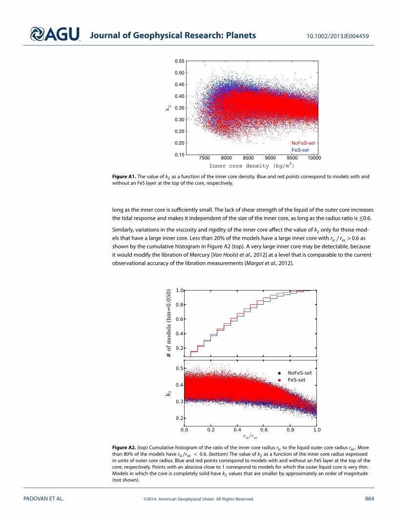
long as the inner core is sufficiently small. The lack of shear strength of the liquid of the outer core increases

the tidal response and makes it independent of the size of the inner core, as long as the radius ratio is ≲0.6.

Similarly, variations in the viscosity and rigidity of the inner core affect the value of k2 only for those mod-

els that have a large inner core. Less than 20% of the models have a large inner core with ric ∕ roc>0.6 as

shown by the cumulative histogram in Figure A2 (top). A very large inner core may be detectable, because

it would modify the libration of Mercury [Van Hoolst et al., 2012] at a level that is comparable to the current

observational accuracy of the libration measurements [Margot et al., 2012].

Figure A2. (top) Cumulative histogram of the ratio of the inner core radius ric to the liquid outer core radius roc. Morethan 80% of the models have ric∕roc < 0.6. (bottom) The value of k2 as a function of the inner core radius expressedin units of outer core radius. Blue and red points correspond to models with and without an FeS layer at the top of thecore, respectively. Points with an abscissa close to 1 correspond to models for which the outer liquid core is very thin.Models in which the core is completely solid have k2 values that are smaller by approximately an order of magnitude(not shown).

PADOVAN ET AL. ©2014. American Geophysical Union. All Rights Reserved. 864

Journal of Geophysical Research: Planets 10.1002/2013JE004459

ReferencesAlterman, Z., H. Jarosch, and C. L. Pekeris (1959), Oscillations of the Earth, Proc. Roy. Soc. London, Ser. A, 252, 80–95,

doi:10.1098/rspa.1959.0138.Anderson, B. J., C. L. Johnson, H. Korth, R. M. Winslow, J. E. Borovsky, M. E. Purucker, J. A. Slavin, S. C. Solomon, M. T. Zuber,

and R. L. McNutt Jr. (2012), Low-degree structure in Mercury’s planetary magnetic field, J. Geophys. Res., 117, E00L12,doi:10.1029/2012JE004159.

Arfken, G. B., and H. J. Weber (2005), Mathematical Methods for Physicists: A Comprehensive Guide, 6th ed., Academic Press, Waltham,Mass.

Biot, M. A. (1954), Theory of stress-strain relations in anisotropic viscoelasticity and relaxation phenomena, J. Appl. Phys., 25, 1385–1391,doi:10.1063/1.1721573.

Borch, R. S., and H. W. Green (1987), Dependence of creep in olivine on homologous temperature and its implications for flow in themantle, Nature, 330, 345–348, doi:10.1038/330345a0.

Cammarano, F., S. Goes, P. Vacher, and D. Giardini (2003), Inferring upper-mantle temperatures from seismic velocities, Phys. Earth Planet.Inter., 138, 197–222, doi:10.1016/S0031-9201(03)00156-0.

Charlier, B., T. L. Grove, and M. T. Zuber (2013), Phase equilibria of ultramafic compositions on Mercury and the origin of thecompositional dichotomy, Earth Planet. Sci. Lett., 363, 50–60, doi:10.1016/j.epsl.2012.12.021.

Christensen, U. R. (2006), A deep dynamo generating Mercury’s magnetic field, Nature, 444, 1056–1058, doi:10.1038/nature05342.Colombo, G. (1966), Cassini’s second and third laws, Astron. J., 71, 891–896, doi:10.1086/109983.Denevi, B. W., et al. (2013), The distribution and origin of smooth plains on Mercury, J. Geophys. Res. Planets, 118, 891–907,

doi:10.1002/jgre.20075.Efroimsky, M. (2012), Bodily tides near spin-orbit resonances, Celestial Mech. Dyn. Astron., 112, 283–330, doi:10.1007/s10569-011-9397-4.Efroimsky, M., and V. Lainey (2007), Physics of bodily tides in terrestrial planets and the appropriate scales of dynamical evolution, J.

Geophys. Res., 112, E12003, doi:10.1029/2007JE002908.Evans, L. G., et al. (2012), Major-element abundances on the surface of Mercury: Results from the MESSENGER Gamma-Ray Spectrometer,

J. Geophys. Res., 117, E00L07, doi:10.1029/2012JE004178.Fegley, B., and A. G. W. Cameron (1987), A vaporization model for iron/silicate fractionation in the Mercury protoplanet, Earth Planet. Sci.

Lett., 82, 207–222, doi:10.1016/0012-821X(87)90196-8.Fei, Y., C. T. Prewitt, H.-K. Mao, and C. M. Bertka (1995), Structure and density of FeS at high pressure and high temperature and the

internal structure of Mars, Science, 268, 1892–1894, doi:10.1126/science.268.5219.1892.Hauck, S. A., II et al. (2013), The curious case of Mercury’s internal structure, J. Geophys. Res. Planets, 118, 1204–1220,

doi:10.1002/jgre.20091.Head, J. W., et al. (2011), Flood volcanism in the northern high latitudes of Mercury revealed by MESSENGER, Science, 333, 1853–1856,

doi:10.1126/science.1211997.Hirschmann, M. M. (2000), Mantle solidus: Experimental constraints and the effects of peridotite composition, Geochem. Geophys.

Geosyst., 1, 1042–1068, doi:10.1029/2000GC000070.Hofmeister, A., and H. Mao (2003), Pressure derivatives of shear and bulk moduli from the thermal Gruneisen parameter and

volume-pressure data, Geochim. Cosmochim. Acta, 67, 1207–1227, doi:10.1016/S0016-7037(02)01289-9.Iess, L., R. A. Jacobson, M. Ducci, D. J. Stevenson, J. I. Lunine, J. W. Armstrong, S. W. Asmar, P. Racioppa, N. J. Rappaport, and P. Tortora

(2012), The tides of Titan, Science, 337, 457–459, doi:10.1126/science.1219631.Jackson, I., U. H. Faul, D. Suetsugu, C. Bina, T. Inoue, and M. Jellinek (2010), Grainsize-sensitive viscoelastic relaxation in olivine: Towards a

robust laboratory-based model for seismological application, Phys. Earth Planet. Inter., 183, 151–163, doi:10.1016/j.pepi.2010.09.005.Konopliv, A. S., and C. F. Yoder (1996), Venusian k2 tidal Love number from Magellan and PVO tracking data, Geophys. Res. Lett., 23,

1857–1860.Konopliv, A. S., S. W. Asmar, W. M. Folkner, Ö. Karatekin, D. C. Nunes, S. E. Smrekar, C. F. Yoder, and M. T. Zuber (2011), Mars

high resolution gravity fields from MRO, Mars seasonal gravity, and other dynamical parameters, Icarus, 211, 401–428,doi:10.1016/j.icarus.2010.10.004.

Konopliv, A. S., et al. (2013), The JPL lunar gravity field to spherical harmonic degree 660 from the GRAIL Primary Mission, J. Geophys. Res.Planets, 118, 1415–1434, doi:10.1002/jgre.20097.

Lemoine, F. G., et al. (2013), High-degree gravity models from GRAIL primary mission data, J. Geophys. Res. Planets, 118, 1676–1698,doi:10.1002/jgre.20118.

Malavergne, V., M. J. Toplis, S. Berthet, and J. Jones (2010), Highly reducing conditions during core formation on Mercury: Implicationsfor internal structure and the origin of a magnetic field, Icarus, 206, 199–209, doi:10.1016/j.icarus.2009.09.001.

Margot, J.-L., S. J. Peale, R. F. Jurgens, M. A. Slade, and I. V. Holin (2007), Large longitude libration of Mercury reveals a molten core,Science, 316, 710–714, doi:10.1126/science.1140514.

Margot, J.-L., S. J. Peale, S. C. Solomon, S. A. Hauck II, F. D. Ghigo, R. F. Jurgens, M. Yseboodt, J. D. Giorgini, S. Padovan, and D. B. Campbell(2012), Mercury’s moment of inertia from spin and gravity data, J. Geophys. Res., 117, E00L09, doi:10.1029/2012JE004161.

Mazarico, E., A. Genova, S. J. Goossens, F. G. Lemoine, D. E. Smith, M. T. Zuber, G. A. Neumann, and S. C. Solomon (2014), The gravity fieldof Mercury from MESSENGER, Lunar Planet. Sci., 45, abstract 1863.

McCoy, T. J., T. L. Dickinson, and G. E. Lofgren (1999), Partial melting of the Indarch (EH4) meteorite: A textural, chemical and phaserelations view of melting and melt migration, Meteorit. Planet. Sci., 34, 735–746, doi:10.1111/j.1945-5100.1999.tb01386.x.

Michel, N. C., S. A. Hauck II, S. C. Solomon, R. J. Phillips, J. H. Roberts, and M. T. Zuber (2013), Thermal evolution of Mercury as constrainedby MESSENGER observations, J. Geophys. Res. Planets, 118, 1033–1044, doi:10.1002/jgre.20049.

Milani, A., A. Rossi, D. Vokrouhlicky, D. Villani, and C. Bonanno (2001), Gravity field and rotation state of Mercury from the BepiColomboRadio Science Experiments, Planet. Space Sci., 49, 1579–1596, doi:10.1016/S0032-0633(01)00095-2.

Moore, W. B., and G. Schubert (2000), Note: The tidal response of Europa, Icarus, 147, 317–319, doi:10.1006/icar.2000.6460.Morgan, J. W., and E. Anders (1980), Chemical composition of Earth, Venus, and Mercury, Proc. Nat. Acad. Sci., 77, 6973–6977,

doi:10.1073/pnas.77.12.6973.Murray, C. D., and S. F. Dermott (1999), Solar System Dynamics, Cambridge Univ. Press, Cambridge, U. K.Nimmo, F., and U. H. Faul (2013), Dissipation at tidal and seismic frequencies in a melt-free, anhydrous Mars, J. Geophys. Res. Planets, 118,

2558–2569, doi:10.1002/2013JE004499.Nimmo, F., U. H. Faul, and E. J. Garnero (2012), Dissipation at tidal and seismic frequencies in a melt-free Moon, J. Geophys. Res., 117,

E09005, doi:10.1029/2012JE004160.

AcknowledgmentsWe thank all the individuals whomade the MESSENGER missionpossible. S.P. and J.-L.M. were par-tially supported by MESSENGERParticipating Scientist Program undergrant NNX09AR45G and by the UCLADivision of Physical Sciences. TheMESSENGER project is supportedby the NASA Discovery Programunder contracts NAS5-97271 to theJohns Hopkins University AppliedPhysics Laboratory and NASW-00002to the Carnegie Institution ofWashington. The comments of theassociate editor Dr. F. Nimmo, of Dr.J. Roberts, and of an anonymousreviewer improved the quality ofthis paper. We thank A. Kavner, J.Mitchell, and G. Schubert for fruitfuland informative discussions.

PADOVAN ET AL. ©2014. American Geophysical Union. All Rights Reserved. 865

Journal of Geophysical Research: Planets 10.1002/2013JE004459

Nittler, L. R., et al. (2011), The major-element composition of Mercury’s surface from MESSENGER X-ray spectrometry, Science, 333,1847–1850, doi:10.1126/science.1211567.

Peale, S. J. (1969), Generalized Cassini’s laws, Astron. J., 74, 483–489, doi:10.1086/110825.Peale, S. J. (1976), Does Mercury have a molten core? Nature, 262, 765–766, doi:10.1038/262765a0.Peplowski, P. N., et al. (2011), Radioactive elements on Mercury’s surface from MESSENGER: Implications for the planet’s formation and

evolution, Science, 333, 1850–1852, doi:10.1126/science.1211576.Rivoldini, A., and T. Van Hoolst (2013), The interior structure of Mercury constrained by the low-degree gravity field and the rotation of

Mercury, Earth Planet. Sci. Lett., 377, 62–72, doi:10.1016/j.epsl.2013.07.021.Rivoldini, A., T. van Hoolst, and O. Verhoeven (2009), The interior structure of Mercury and its core sulfur content, Icarus, 201, 12–30,

doi:10.1016/j.icarus.2008.12.020.Siivola, J., and R. Schmid (2007), List of mineral abbreviations, recommendations by the IUGS subcommission on the systematics of

metamorphic rocks. [Available at Electronic Source: http://www.bgs.ac.uk/scmr/docs/papers/paper_12.pdf.]Smith, D. E., et al. (2012), Gravity field and internal structure of Mercury from MESSENGER, Science, 336, 214–217, doi:10.1126/sci-

ence.1218809.Sobolev, S. V., and A. Y. Babeyko (1994), Modeling of mineralogical composition, density and elastic wave velocities in anhydrous

magmatic rocks, Surv. Geophys., 15, 515–544, doi:10.1007/BF00690173.Stockstill-Cahill, K. R., T. J. McCoy, L. R. Nittler, S. Z. Weider, and S. A. Hauck II (2012), Magnesium-rich crustal compositions on Mercury:

Implications for magmatism from petrologic modeling, J. Geophys. Res., 117, E00L15, doi:10.1029/2012JE004140.Taylor, G. J., and E. R. D. Scott (2005), Mercury, in Treatise on Geochemistry, Vol. 1: Meteorites, Comets and Planets, edited by A. M. Davis, H.

D. Holland, and K. K. Turekian, pp. 477–485, Elsevier, Amsterdam, The Netherlands, doi:10.1016/B0-08-043751-6/01071-9.Tosi, N., M. Grott, A.-C. Plesa, and D. Breuer (2013), Thermochemical evolution of Mercury’s interior, J. Geophys. Res. Planets, 118,

2474–2487, doi:10.1002/jgre.20168.Turcotte, D. L., and G. Schubert (2002), Geodynamics, 2nd ed., Cambridge Univ. Press, Cambridge, U. K., doi:10.2277/0521661862.Urakawa, S., K. Someya, H. Terasaki, T. Katsura, S. Yokoshi, K.-I. Funakoshi, W. Utsumi, Y. Katayama, Y.-I. Sueda, and T. Irifune (2004), Phase

relationships and equations of state for FeS at high pressures and temperatures and implications for the internal structure of Mars,Phys. Earth Planet. Inter., 143, 469–479, doi:10.1016/j.pepi.2003.12.015.

Vacher, P., A. Mocquet, and C. Sotin (1998), Computation of seismic profiles from mineral physics: The importance of the non-olivinecomponents for explaining the 660 km depth discontinuity, Phys. Earth Planet. Inter., 106, 277–300.

Van Hoolst, T., and C. Jacobs (2003), Mercury’s tides and interior structure, J. Geophys. Res., 108, 5121, doi:10.1029/2003JE002126.Van Hoolst, T., A. Rivoldini, R.-M. Baland, and M. Yseboodt (2012), The effect of tides and an inner core on the forced longitudinal libration

of Mercury, Earth Planet. Sci. Lett., 333, 83–90, doi:10.1016/j.epsl.2012.04.014.Verhoeven, O., et al. (2005), Interior structure of terrestrial planets: Modeling Mars’ mantle and its electromagnetic, geodetic, and seismic

properties, J. Geophys. Res., 110, E04009, doi:10.1029/2004JE002271.Wasson, J. T. (1988), The building stones of the planets, in Mercury, edited by F. Vilas, C. R. Chapman, and M. S. Matthews, pp. 622–650,

Univ. of Ariz. Press, Tucson, Ariz.Watt, J. P., G. F. Davies, and R. J. O’Connell (1976), The elastic properties of composite materials, Rev. Geophys. Space Phys., 14, 541–563,

doi:10.1029/RG014i004p00541.Weider, S. Z., L. R. Nittler, R. D. Starr, T. J. McCoy, K. R. Stockstill-Cahill, P. K. Byrne, B. W. Denevi, J. W. Head, and S. C. Solomon (2012),

Chemical heterogeneity on Mercury’s surface revealed by the MESSENGER X-Ray Spectrometer, J. Geophys. Res., 117, E00L05,doi:10.1029/2012JE004153.

Wolf, D. (1994), Lamé’s problem of gravitational viscoelasticity: The isochemical, incompressible planet, Geophys. J. Int., 116, 321–348,doi:10.1111/j.1365-246X.1994.tb01801.x.

Yoder, C. F., A. S. Konopliv, D. N. Yuan, E. M. Standish, and W. M. Folkner (2003), Fluid core size of Mars from detection of the solar tide,Science, 300, 299–303, doi:10.1126/science.1079645.

Zhao, Y.-H., M. E. Zimmerman, and D. L. Kohlstedt (2009), Effect of iron content on the creep behavior of olivine: 1. Anhydrous conditions,Earth Planet. Sci. Lett., 287, 229–240, doi:10.1016/j.epsl.2009.08.006.

Zolotov, M. Y., A. L. Sprague, S. A. Hauck II, L. R. Nittler, S. C. Solomon, and S. Z. Weider (2013), The redox state, FeO content, and originof sulfur-rich magmas on Mercury, J. Geophys. Res. Planets, 118, 138–146, doi:10.1029/2012JE004274.

Zuber, M. T., D. E. Smith, D. H. Lehman, T. L. Hoffman, S. W. Asmar, and M. M. Watkins (2013), Gravity Recovery and Interior Laboratory(GRAIL): Mapping the lunar interior from crust to core, Space Sci. Rev., 178, 3–24, doi:10.1007/s11214-012-9952-7.

PADOVAN ET AL. ©2014. American Geophysical Union. All Rights Reserved. 866