The Time for Austerity: Estimating the Average Treatment ...faculty.smu.edu/millimet/classes/eco7377/papers/jorda taylor 2015.pdf · THE TIME FOR AUSTERITY: ESTIMATING THE AVERAGE

THE TIME FOR AUSTERITY: ESTIMATING THE AVERAGETREATMENT EFFECT OF FISCAL POLICY*

�Oscar Jord�a and Alan M. Taylor

After the Global Financial Crisis, a controversial rush to fiscal austerity followed in many countries.Yet research on the effects of austerity on macroeconomic aggregates was and still is unsettled, miredby the difficulty of identifying multipliers from observational data. This article, reconciles seeminglydisparate estimates of multipliers within a unified and state-contingent framework. We achieveidentification of causal effects with new propensity-score based methods for time series data. Usingthis novel approach, we show that austerity is always a drag on growth, and especially so in depressedeconomies: a 1% of GDP fiscal consolidation translates into a loss of 3.5% of real GDP over five yearswhen implemented in a slump, rather than just 1.8% in a boom.

I solemnly affirm and believe, if a hundred or a thousand men of the same age,same temperament and habits, together with the same surroundings, wereattacked at the same time by the same disease, that if one half followed theprescriptions of the doctors of the variety of those practising at the presentday, and that the other half took no medicine but relied on Nature’s instincts,I have no doubt as to which half would escape. – A doctor, quoted by Petrarchin his letter to Boccaccio, 1364 (Donaldson, 2016).

The boom, not the slump, is the right time for austerity at the Treasury.– J. M. Keynes (1937)

In 1809 on a battlefield in Portugal, in a defining experiment in epidemiologicalhistory, a Scottish surgeon and his colleagues attempted what some believe to havebeen the first recognisable medical trial, a test of the effectiveness of bloodletting on asample of 366 soldiers allocated into treatment and control groups by alternation. Thecure was shown to be bogus. Tests of this sort heralded the beginning of the end ofpremodern medicine, vindicating sceptics like Petrarch for whom the idea of a fair trialwas a mere thought experiment. Yet, even with alternation, allocation bias – i.e.‘insufficient randomisation’ – remained pervasive in poor experimental designs (e.g.via foreknowledge of assignment) and the intellectual journey was only completed inthe 1940s with the landmark British Medical Research Council trials of patulin and

* Corresponding author: Alan M. Taylor, Department of Economics and Graduate School of Management,University of California, Davis, CA 95616, USA. Email: [email protected].

The views expressed herein are solely the responsibility of the authors and should not be interpreted asreflecting the views of the Federal Reserve Bank of San Francisco or the Board of Governors of the FederalReserve System. We thank three referees and the editor as well as seminar participants at the Federal ReserveBank of San Francisco, the Swiss National Bank, the NBER Summer Institute, the Bank for InternationalSettlements, the European Commission and HM Treasury for helpful comments and suggestions. We areparticularly grateful to Daniel Leigh for sharing data and Early Elias for outstanding research assistance. Allerrors are ours.

[ 219 ]

The Economic Journal, 126 (February), 219–255. Doi: 10.1111/ecoj.12332 © 2015 Royal Economic Society. Published by John Wiley & Sons, 9600

Garsington Road, Oxford OX4 2DQ, UK and 350 Main Street, Malden, MA 02148, USA.

streptomycin. Ever since the randomised controlled trial has been the foundation ofevidence-based medicine.1

Is a similar evidence-based macroeconomics possible and what can it learn from thisnoble scientific tradition? Ideas from the experimental approach bridge medicine,epidemiology, and statistics, and they have slowly infected empirical economics,although mostly on the micro side.2 In this article, we delve into the experimentaltoolkit so as to re-examine a key issue for macroeconomics, the need to ensuretreatments are somehow re-randomised in non-experimental data. We do this in thecontext of the foremost academic and policy dispute of the day – the effects of fiscalpolicy shocks on output; see, in particular, Alesina and Ardagna (2010) and Guajardoet al. (2014).3

Identification of the effects of fiscal consolidation in empirical studies has broadlytaken one of two forms. In the context of a vector autoregression, one option is toachieve identification based on exclusion restrictions. In practice, these restrictions areroughly equivalent to a regression-control strategy based on a limited number ofobservable controls and (usually) a linear conditional mean assumption. Examples ofthis strand of the literature include Alesina and Perotti (1995), Perotti (1999) andMountford and Uhlig (2009). The other strand of the literature has approached theidentification problem through instrumental variables. Examples of this approachinclude Auerbach and Gorodnichenko (2012, 2013), Mertens and Ravn (2013, 2014)and Owyang et al. (2013).

Following a new and arguably more promising direction, we take a third fork on theroad to identification based on the Rubin Causal Model. This approach has theattractive features of being semi-parametric (and hence flexible with respect to thefunctional form), providing better control for observables, and offering a more reliablealternative when the putative instrumental variables for policy action are themselvespossibly endogenous. Tests of instrument validity are well-known to have low power(Cameron and Trivedi, 2005) but, more importantly, formal testing is not an optionwhen we are in the case of exact identification.

We find that, on average, fiscal consolidations generate a drag on GDP growth. Theeffect is also state dependent: if a 1% of GDP fiscal consolidation is imposed in a slumpthen it results in a real GDP loss of around 3.5% over five years, rather than just 1.8% ina boom. We arrive at this conclusion by carefully constructing an encompassingframework that allows us to evaluate the type of approach followed by several recentarticles in the literature (to be discussed in detail shortly) to improve comparability

1 See Chalmers (2005, 2011), who discusses Petrarch, bloodletting and the MRC clinical trials.2 Angrist and Pischke (2010, p. 5) judge that ‘progress has been slower in empirical macro’. The fear that

standard empirical practices would not work, especially for aggregate economic questions, goes back a longway, at least to J. S. Mill (1836, p. 18), who favoured a priori reasoning alone, arguing that: ‘There is a propertycommon to almost all the moral sciences, and by which they are distinguished from many of the physical; thisis, that it is seldom in our power to make experiments in them’.

3 Ironically enough, fiscal policy debates are now littered with medical metaphors. In 2011 GermanFinance Minister Wolfgang Sch€auble wrote in The Financial Times, that ‘austerity is the only cure for theEurozone’; while Paul Krugman, at The New York Times, likened it to ‘economic bloodletting’. In the FT,Martin Wolf, cautioned that ‘the idea that treatment is right irrespective of what happens to the patient fallsinto the realm of witch-doctoring, not science’. Martin Taylor, former head of Barclays, put it bluntly:‘Countries are being enrolled, like it or not, in the economic equivalent of clinical trials’.

© 2015 Royal Economic Society.

220 TH E E CONOM I C J O U RN A L [ F E B R U A R Y

with the methods we introduce in this article. In addition to accommodating existingmethods, the framework allows us to address the identification concerns we uncover viathe application of an estimator from the family of ‘doubly robust’ augmented inverse-propensity-score weighted regression adjustment methods (Robins et al., 1994;Scharfstein et al., 1999; Robins, 2000; Hirano et al., 2003; Imbens, 2004; Luncefordand Davidian, 2004; Glynn and Quinn, 2010).

To provide more texture to our results, we evaluate the UK austerity programmeimplemented by the Coalition Government after the 2010 election. The GlobalFinancial Crisis struck the US and the UK in a similar way and these economies ran onparallel trajectories until 2010. Thereafter the UK experienced a second slowdownwhile the US continued to grow. Using our estimates we compute how much of theslowdown could be attributed to the austerity programme; we find it to be a verysignificant contribution (rising to 3.1% of GDP in 2013) and larger than officialestimates. Thus, better models, with state-dependent features, could improve officialfiscal policy analyses going forward.

1. The Austerity Debate: A Road Map

Are fiscal consolidations expansionary, neutral, or contractionary? In order to answerthis question and understand the different answers the literature has arrived at so far,we proceed in a series of incremental stages.

First, we use the OECD annual panel data set adopted in two recent high-profile yetseemingly irreconcilable studies. The ‘expansionary austerity’ idea has come to beassociated with the paper by Alesina and Ardagna (2010, henceforth AA) an ideaperhaps dating back to at least Giavazzi and Pagano (1990). On the opposite side, theIMF team of Guajardo et al. (2014, henceforth GLP) reached the opposite conclusionof ‘contractionary austerity’. By juxtaposing these two papers we are not implying thatthe literature falls evenly or comprehensively within these two camps. We use thecontraposition as a rhetorical device much like Perotti (2013), who presents a luciddiscussion of the empirical pitfalls in this research area.

Second, we use Jord�a (2005) local projections (LPs), rather than structural vectorauto regressions (SVARs). The reason is that, among other advantages that we willdiscuss momentarily, LPs are a convenient pedestal on which all extensions of existingestimation methods can rest. The unified framework provides the reader a way tocompare the results across a set of nested estimation strategies.

LPs provide a flexible semi-parametric regression control strategy to estimatedynamic multipliers and include, as a special case, impulse responses calculated withan SVAR. LPs accommodate possibly non-linear, or state-dependent responses easily,and indeed we find that the effects of fiscal policy can be very different in the boomand the slump, as emphasised by Keynes in the 1930s. State-dependent multipliersbased on LPs have been taken up in some very recent papers (Auerbach andGorodnichenko, 2012, 2013, for the US and OECD; Owyang et al., 2013, for the USand Canada). Other recent papers on state-dependent multipliers, using variousmeasures of slack, include Barro and Redlick (2011) and Nakamura and Steinsson(2014). For a critical survey see Parker (2011). Long ago, Perotti (1999) explored theidea of ‘expansionary austerity’ with state-dependent multipliers.


2016] T H E T I M E F O R AU S T E R I T Y 221

We calculate the impact of fiscal policy shocks based on LPs using the AA measure ofpolicy, the change in the cyclically-adjusted primary balance (d.CAPB).4 When werestrict attention to ‘large’ shocks (changes in CAPB larger in magnitude than 1.5% ofGDP, which is the benchmark cutoff value used by AA and proposed earlier by Alesinaand Perotti, 1995), we replicate the ‘expansionary austerity’ result. However, when wecondition on the state of the economy, we find that this result is driven entirely by whathappens during a boom. The expansionary effects of fiscal consolidation evaporatewhen the economy is in a slump.

Third, we then use instrumental variable (IV) estimation of the LPs to account forunobserved confounders. Specifically, we instrument the cyclically-adjusted primarybalance using the IMF’s narrative measure of an exogenous fiscal consolidation inGLP. This type of ‘narrative-based identification’ has been applied by, e.g. Romer andRomer (1989, 1997), Ramey and Shapiro (1998) and Mertens and Ravn (2013, 2014).Our IV estimation then turns out to replicate the flavour of the GLP results: austerity iscontractionary, and strongly so in slumps.

Fourth, we show that the proposed IMF narrative instrumental variable has asignificant forecastable element driven by plausible state variables, such as the debt-to-GDP level, the cyclical level or rate of growth of real GDP, and the lagged treatmentindicator itself (since austerity programmes are typically persistent, multi-year affairs).5

Formal testing of instrument validity is not possible since we have exact (not over-)identification. However, the evidence that we provide calls into question the validity ofthe narrative instrumental variable. As noted above in the history of medicine and aswith any efforts to construct a narrative policy variable that is exogenous, one has toworry about the possibility that treatment is still contaminated by endogeneity, whichwould impart allocation bias to any estimates.6

Fifth, in order to purge the remaining allocation bias, we use inverse probabilityweighting (IPW) estimation based on a prediction model of the narrative policyvariable to estimate the LP responses. We consider the IMF narrative policy variable asa ‘fiscal treatment’ – i.e. a binary indicator rather than a continuous variable – and weare interested in characterising a dynamic average treatment effect (ATE). In newwork, Angrist et al. (2013) introduce IPW estimators in a time series context tocalculate the dynamic ATE responses to policy interventions. We follow a slightlydifferent approach using augmented regression-adjusted estimation instead, denotedAIPW, which combines IPW with regression control and adjusts the estimator toachieve semi-parametric efficiency (Lunceford and Davidian, 2004). Our AIPWestimator falls into the broad class of ‘doubly robust’ estimators of which Robins et al.(1994) is perhaps the earliest reference (Scharfstein et al., 1999; Robins, 2000; Hiranoet al., 2003; Imbens, 2004; Lunceford and Davidian, 2004; Glynn and Quinn, 2010).

4 The d.CAPB measure used by AA is based on Blanchard (1993). The construction of this variable consistsof adjusting for cyclical fluctuations using the unemployment rate.

5 The potential endogeneity of fiscal consolidation episodes has been noted by other authors. Forexample, Ardagna (2004) uses political variables as an exogenous driver for consolidation in a GLSsimultaneous equation model of growth and consolidation for the period 1975–2002. Hern�andez de Cos andMoral-Benito (2013) use economic variables as instruments.

6 For example, in the debate over the use of narrative methods to assess monetary policy, see the exchangebetween Leeper (1997) and Romer and Romer (1997).



The ‘doubly robust’ property means that consistency of the estimated ATE can beproved in the special cases where either the propensity score model and/or theconditional mean is correctly specified; Monte Carlo evidence also suggests that theestimator performs better than alternatives even in more general cases too.

The remainder of the article expands on each of these stages in turn.

2. Replicating Expansionary Austerity: OLS Results

Our first estimates use OLS estimation with the LP method, based on what is thetraditional variable in the literature, the change in the cyclically adjusted primarybalance (denoted d.CAPB), the same variable used by Alesina and Perotti (1995) andby AA, and used as a reference point by GLP in the IMF study. The local projection isdone from year 0, when a policy change is assumed to be announced, with the fiscalimpacts first felt in year 1, consistent with the timing in GLP. The LP output forecastpath is constructed out to year 5, deviations from year 0 levels are shown and also thesum of these deviations, or ‘lost output’, across all of those five years.

To create a benchmark estimating equation that mimics the standard setup in theliterature, the typical LP equation that we estimate has the form:

yi;tþh � yi;t ¼ ahi þ KhDi;tþ1 þ bhL0Dyi;t þ bhL1Dyi;t�1 þ bhCyCi;t þ vi;tþh; (1)

for h = 1, . . . , 5, and where yi;tþh � yi;t denotes the cumulative change from time t tot + h in 100 times the log of real GDP, the ahi are country-fixed effects, and Di;t denotesthe d.CAPB policy variable (measured from time t to time t + 1 given the assumedtiming of the announcement and implementation of fiscal plans). Finally, to controlfor reversion to the potential output trend, the term yCi;t is the output gap, denoting thecyclical component of GDP, and it is proxied here by deviations of log real GDP froman HP trend estimated with a smoothing parameter of k = 100. We use the subscriptsL0 and L1 for the b parameters associated to Dyi;t�l for l = 0, 1 so as not to confusethem with the j = 1, 0 treatment-control index that we will use later.

Our choice of using the HP filter with k = 100 was justified by a series of experimentsundertaken with US postwar data (from FRED) which showed that a relatively highsmoothing parameter was needed if the proposed proxy series (HP filtered log realGDP) was to come close to matching the official CBO output gap series. We alsoreplicated this type of analysis using a bandpass filter tuned to various frequencies andthe conclusions were very similar. That is to say, we found that the conventional filterfrequencies typically used in the business cycle literature are too low to provide a goodmatch with the output gap, which is what we want in our model so as to control forreversion to trend. These experiments are available from the authors upon request.

The specification (1) nests themain elements in AA andGLP to facilitate comparisonsof our results with theirs. The coefficient Kh from expression (1) is the parametergoverning the impact of the continuous policy treatment measured by d.CAPB andcorresponds to the constrained version of expression (7) below in Section 5, where wehave rearranged that expression to get a direct estimate of the average response to policyintervention Kh from the regression output, but it is otherwise specified the same way.

Table 1 reports estimates based on expression (1). Estimated log real GDP impacts(9 100) for each year are reported in columns 1–5 and the five-year sum of the



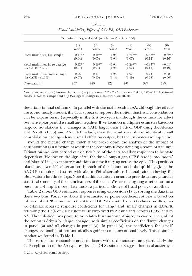
deviations in final column 6. In parallel with the main result in AA, although the effectsare economically modest, the data appear to support the notion that fiscal consolidationcan be expansionary (especially in the first two years), although the cumulative effectover a five year period is small and negative. If we focus on multiplier estimates based onlarge consolidations (i.e. changes in CAPB larger than 1.5% of GDP using the Alesinaand Perotti (1995) and AA cutoff value), then the results are almost identical. Smallconsolidation packages have a small effect on output, but the estimates are imprecise.

Would the picture change much if we broke down the analysis of the impact ofconsolidation as a function of whether the economy is experiencing a boom or a slump?Estimation was next carried out on two bins of the data to allow responses to be statedependent. We sort on the sign of yC , the time-0 output gap (HP filtered) into ‘boom’and ‘slump’ bins, to capture conditions at time 0 varying across the cycle. This partitionplaces just over 200 observations in each of the ‘boom’ and ‘slump’ bins, given theAA-GLP combined data set with about 450 observations in total, after allowing forobservations lost due to lags. Note that this partition is meant to provide amore granularstatistical summary of the main features of the data. We are not arguing whether or not aboom or a slump is more likely under a particular choice of fiscal policy or another.

Table 2 shows OLS estimated responses using expression (1) by sorting the data intothese two bins. Panel (a) shows the estimated response coefficient at year h based onvalues of d.CAPB common to the AA and GLP data sets. Panel (b) shows results whenwe estimate separate response coefficients for ‘large’ and ‘small’ changes in d.CAPB,following the 1.5% of GDP cutoff value employed by Alesina and Perotti (1995) and byAA. These distinctions prove to be relatively unimportant since, as can be seen, all ofthe action is driven by ‘large’ changes, with similar coefficients on the ‘large’ changesin panel (b) and all changes in panel (a). In panel (b), the coefficients for ‘small’changes are small and not statistically significant at conventional levels. This is similarto what we found in Table 1.

The results are reasonable and consistent with the literature, and particularly theGLP replication of the AA-type results. The OLS estimates suggest that fiscal austerity is

Table 1

Fiscal Multiplier, Effect of d.CAPB, OLS Estimates

Deviation in log real GDP (relative to Year 0, 9 100)

(1) (2) (3) (4) (5) (6)Year 1 Year 2 Year 3 Year 4 Year 5 Sum

Fiscal multiplier, full sample 0.11** 0.12** �0.04 �0.21*** �0.32** �0.42**(0.04) (0.05) (0.04) (0.07) (0.12) (0.16)

Fiscal multiplier, large changein CAPB (>1.5%)

0.12** 0.13** �0.04 �0.23*** �0.33** �0.41*(0.04) (0.05) (0.04) (0.07) (0.12) (0.19)

Fiscal multiplier, small changein CAPB (≤1.5%)

0.06 0.11 0.03 �0.07 �0.23 �0.53(0.07) (0.15) (0.14) (0.19) (0.28) (0.50)

Observations 457 440 423 406 389 389

Notes. Standarderrors (clusteredby country) inparentheses. ***/**/* Indicatep < 0.01/0.05/0.10.Additionalcontrols: cyclical component of y, two lags of change in y, country fixed effects.



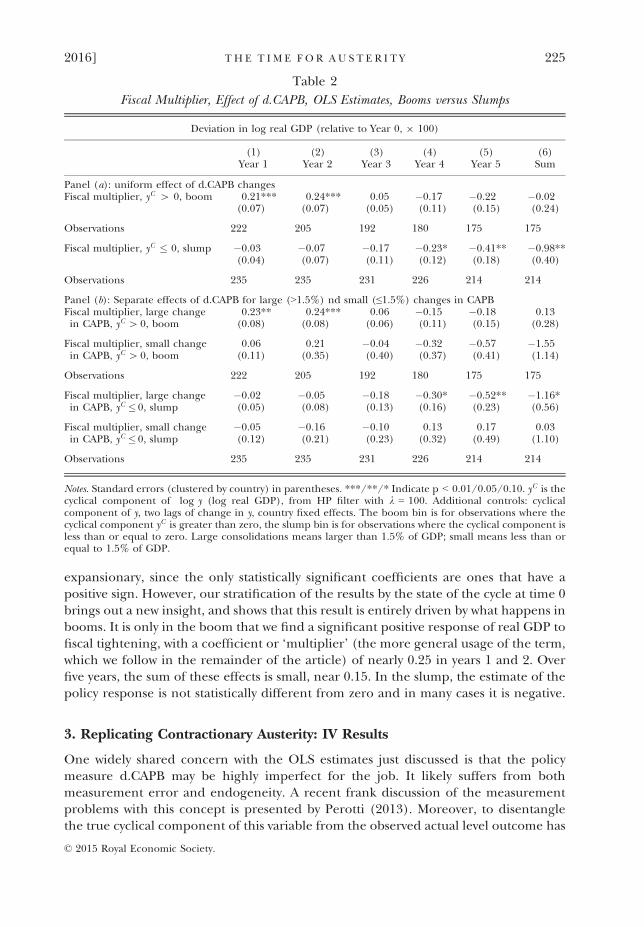
expansionary, since the only statistically significant coefficients are ones that have apositive sign. However, our stratification of the results by the state of the cycle at time 0brings out a new insight, and shows that this result is entirely driven by what happens inbooms. It is only in the boom that we find a significant positive response of real GDP tofiscal tightening, with a coefficient or ‘multiplier’ (the more general usage of the term,which we follow in the remainder of the article) of nearly 0.25 in years 1 and 2. Overfive years, the sum of these effects is small, near 0.15. In the slump, the estimate of thepolicy response is not statistically different from zero and in many cases it is negative.

3. Replicating Contractionary Austerity: IV Results

One widely shared concern with the OLS estimates just discussed is that the policymeasure d.CAPB may be highly imperfect for the job. It likely suffers from bothmeasurement error and endogeneity. A recent frank discussion of the measurementproblems with this concept is presented by Perotti (2013). Moreover, to disentanglethe true cyclical component of this variable from the observed actual level outcome has

Table 2

Fiscal Multiplier, Effect of d.CAPB, OLS Estimates, Booms versus Slumps



Panel (a): uniform effect of d.CAPB changesFiscal multiplier, yC [ 0, boom 0.21*** 0.24*** 0.05 �0.17 �0.22 �0.02

(0.07) (0.07) (0.05) (0.11) (0.15) (0.24)

Observations 222 205 192 180 175 175

Fiscal multiplier, yC � 0, slump �0.03 �0.07 �0.17 �0.23* �0.41** �0.98**(0.04) (0.07) (0.11) (0.12) (0.18) (0.40)

Observations 235 235 231 226 214 214

Panel (b): Separate effects of d.CAPB for large (>1.5%) nd small (≤1.5%) changes in CAPBFiscal multiplier, large changein CAPB, yC [ 0, boom

0.23** 0.24*** 0.06 �0.15 �0.18 0.13(0.08) (0.08) (0.06) (0.11) (0.15) (0.28)

Fiscal multiplier, small changein CAPB, yC [ 0, boom

0.06 0.21 �0.04 �0.32 �0.57 �1.55(0.11) (0.35) (0.40) (0.37) (0.41) (1.14)

Observations 222 205 192 180 175 175

Fiscal multiplier, large changein CAPB, yC � 0, slump

�0.02 �0.05 �0.18 �0.30* �0.52** �1.16*(0.05) (0.08) (0.13) (0.16) (0.23) (0.56)

Fiscal multiplier, small changein CAPB, yC � 0, slump

�0.05 �0.16 �0.10 0.13 0.17 0.03(0.12) (0.21) (0.23) (0.32) (0.49) (1.10)

Observations 235 235 231 226 214 214

Notes. Standard errors (clustered by country) in parentheses. ***/**/* Indicate p < 0.01/0.05/0.10. yC is thecyclical component of log y (log real GDP), from HP filter with k = 100. Additional controls: cyclicalcomponent of y, two lags of change in y, country fixed effects. The boom bin is for observations where thecyclical component yC is greater than zero, the slump bin is for observations where the cyclical component isless than or equal to zero. Large consolidations means larger than 1.5% of GDP; small means less than orequal to 1.5% of GDP.



to rely on modelling assumptions about the sensitivity of taxes and revenues to thecycle – effects which may be only imprecisely estimated and which may not be stableover time or across countries. If that attempt at purging the cyclical part of the variablestill leaves some endogenous variation in d.CAPB, then the implicit assumption ofexogeneity needed for a causal estimate and policy analysis would be violated.

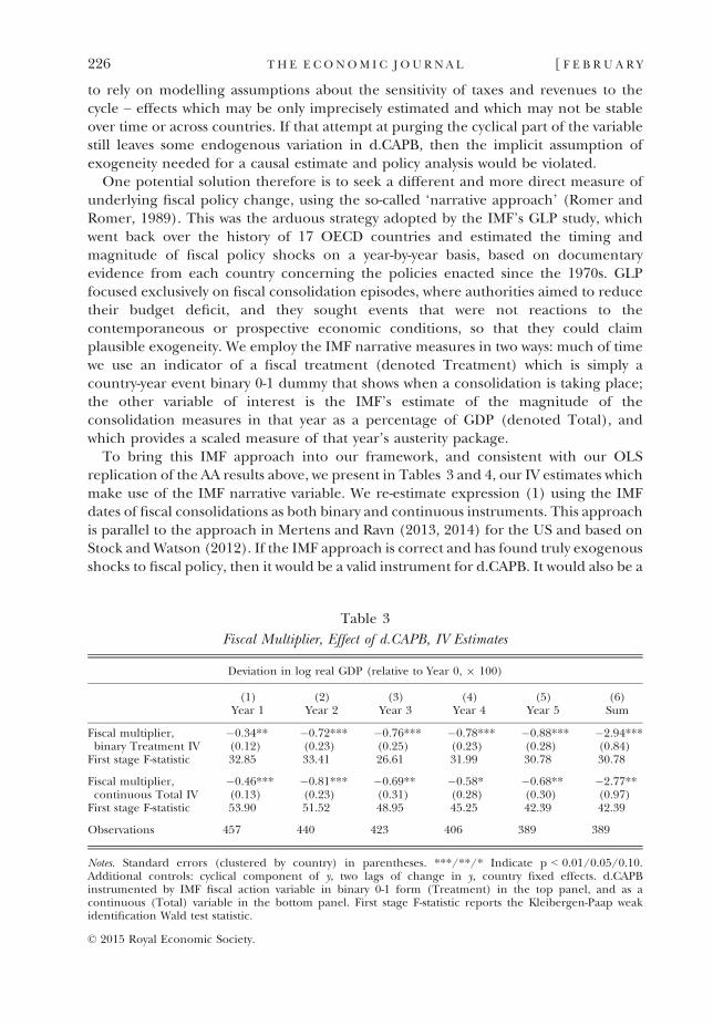
One potential solution therefore is to seek a different and more direct measure ofunderlying fiscal policy change, using the so-called ‘narrative approach’ (Romer andRomer, 1989). This was the arduous strategy adopted by the IMF’s GLP study, whichwent back over the history of 17 OECD countries and estimated the timing andmagnitude of fiscal policy shocks on a year-by-year basis, based on documentaryevidence from each country concerning the policies enacted since the 1970s. GLPfocused exclusively on fiscal consolidation episodes, where authorities aimed to reducetheir budget deficit, and they sought events that were not reactions to thecontemporaneous or prospective economic conditions, so that they could claimplausible exogeneity. We employ the IMF narrative measures in two ways: much of timewe use an indicator of a fiscal treatment (denoted Treatment) which is simply acountry-year event binary 0-1 dummy that shows when a consolidation is taking place;the other variable of interest is the IMF’s estimate of the magnitude of theconsolidation measures in that year as a percentage of GDP (denoted Total), andwhich provides a scaled measure of that year’s austerity package.

To bring this IMF approach into our framework, and consistent with our OLSreplication of the AA results above, we present in Tables 3 and 4, our IV estimates whichmake use of the IMF narrative variable. We re-estimate expression (1) using the IMFdates of fiscal consolidations as both binary and continuous instruments. This approachis parallel to the approach in Mertens and Ravn (2013, 2014) for the US and based onStock andWatson (2012). If the IMF approach is correct and has found truly exogenousshocks to fiscal policy, then it would be a valid instrument for d.CAPB. It would also be a

Table 3

Fiscal Multiplier, Effect of d.CAPB, IV Estimates



Fiscal multiplier,binary Treatment IV

�0.34** �0.72*** �0.76*** �0.78*** �0.88*** �2.94***(0.12) (0.23) (0.25) (0.23) (0.28) (0.84)

First stage F-statistic 32.85 33.41 26.61 31.99 30.78 30.78

Fiscal multiplier,continuous Total IV

�0.46*** �0.81*** �0.69** �0.58* �0.68** �2.77**(0.13) (0.23) (0.31) (0.28) (0.30) (0.97)


Observations 457 440 423 406 389 389

Notes. Standard errors (clustered by country) in parentheses. ***/**/* Indicate p < 0.01/0.05/0.10.Additional controls: cyclical component of y, two lags of change in y, country fixed effects. d.CAPBinstrumented by IMF fiscal action variable in binary 0-1 form (Treatment) in the top panel, and as acontinuous (Total) variable in the bottom panel. First stage F-statistic reports the Kleibergen-Paap weakidentification Wald test statistic.



potentially strong instrument: the raw correlation between d.CAPB (year 1 versus year 0)and Treatment (in year 1) is 0.31 and a bivariate regression has an F-statistic of over 50;the same applies when Treatment is replaced by Total (in year 1).

We begin by re-estimating the full sample specification reported in the top panel ofTable 1 using instrumental variables in two ways. First we use the IMF narrativevariables on dates of fiscal consolidation as a binary instrument (first row). Second, fora continuous IV we use the size of the consolidation identified by the IMF (secondrow). The results are reported in Table 3. Strikingly, the message here completelyoverturns the findings in Table 1. This is of course a well known problem, consistentwith the pronounced divergence between the AA and GLP results. Fiscal consolidationis unambiguously contractionary. Using the sum of coefficients reported in column (6)of Table 3, for every 1% in fiscal consolidation, the path of real GDP is pushed down byover 0.57% each year on average over the five subsequent years. This result is notsensitive to whether we use the binary or continuous instrument.

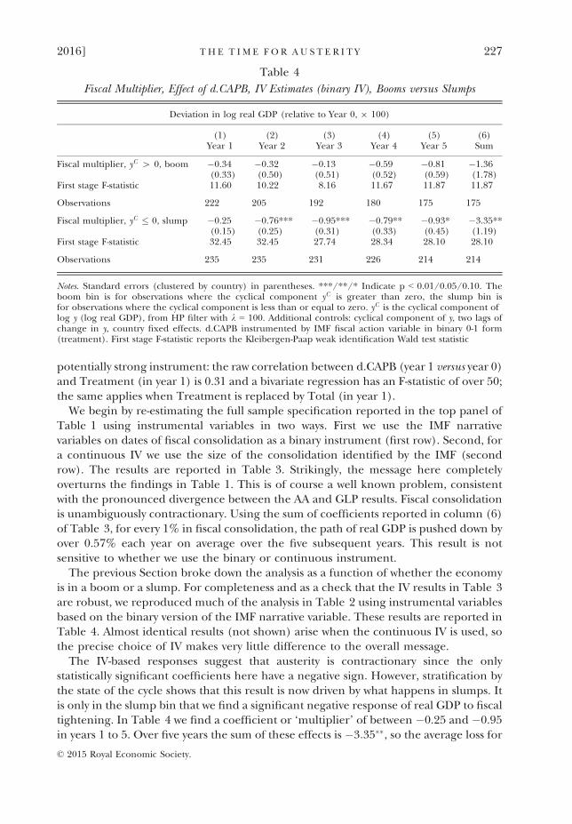
The previous Section broke down the analysis as a function of whether the economyis in a boom or a slump. For completeness and as a check that the IV results in Table 3are robust, we reproduced much of the analysis in Table 2 using instrumental variablesbased on the binary version of the IMF narrative variable. These results are reported inTable 4. Almost identical results (not shown) arise when the continuous IV is used, sothe precise choice of IV makes very little difference to the overall message.

The IV-based responses suggest that austerity is contractionary since the onlystatistically significant coefficients here have a negative sign. However, stratification bythe state of the cycle shows that this result is now driven by what happens in slumps. Itis only in the slump bin that we find a significant negative response of real GDP to fiscaltightening. In Table 4 we find a coefficient or ‘multiplier’ of between �0.25 and �0.95in years 1 to 5. Over five years the sum of these effects is �3:35��, so the average loss for

Table 4

Fiscal Multiplier, Effect of d.CAPB, IV Estimates (binary IV), Booms versus Slumps



Fiscal multiplier, yC [ 0, boom �0.34 �0.32 �0.13 �0.59 �0.81 �1.36(0.33) (0.50) (0.51) (0.52) (0.59) (1.78)


Observations 222 205 192 180 175 175

Fiscal multiplier, yC � 0, slump �0.25 �0.76*** �0.95*** �0.79** �0.93* �3.35**(0.15) (0.25) (0.31) (0.33) (0.45) (1.19)


Observations 235 235 231 226 214 214

Notes. Standard errors (clustered by country) in parentheses. ***/**/* Indicate p < 0.01/0.05/0.10. Theboom bin is for observations where the cyclical component yC is greater than zero, the slump bin isfor observations where the cyclical component is less than or equal to zero. yC is the cyclical component oflog y (log real GDP), from HP filter with k = 100. Additional controls: cyclical component of y, two lags ofchange in y, country fixed effects. d.CAPB instrumented by IMF fiscal action variable in binary 0-1 form(treatment). First stage F-statistic reports the Kleibergen-Paap weak identification Wald test statistic



a 1% of GDP fiscal consolidation is to depress the output level by about �0.67% peryear over this horizon.

4. Endogenous Austerity: Is the Narrative Instrument Valid?

So far we have briefly replicated the current state of the literature but this is not entirelypointless. It serves to show that the LP framework can capture different sides of thedebate in a uniform empirical design, on a consistent data sample, allowing us to focuson how differences in estimation and identification assumptions lead to different results.It also shows how the LP estimation method makes it very easy to allow for non-linearityand do a stratification of results; here we found significant variations in responses acrossbins designed to capture variations in the state of the economy from boom to slump. Wefound that indeed fiscal impacts vary considerably across these states in a manner that isintuitive and not unexpected: the output response to fiscal austerity is less favourable theweaker is the economy. Does this mean that Keynes was right?

Before drawing any conclusions we evaluate whether the IMF narrative variablemight be a legitimate instrument. Have we identified the causal effect of fiscalconsolidations on output? We cannot formally test the validity of the IMF narrativeinstrument since the LPs are just identified. However, if the IMF’s narrative variablecan be predicted by excluded controls and those controls are correlated with theoutcome, at a minimum the excluded controls should be added to the regression. Atworst, predictability points to having failed to resolve the allocation bias in ourestimates – episodes of consolidation identified by the IMF might be simply anendogenous response by the fiscal authority. This possible shortcoming of the‘narrative identification’ strategy has been noted before in the context of monetarypolicy (Leeper, 1997) and we have the same concern here. To address this issue wereport three diagnostic tests in this Section in Tables 5, 6 and 7.

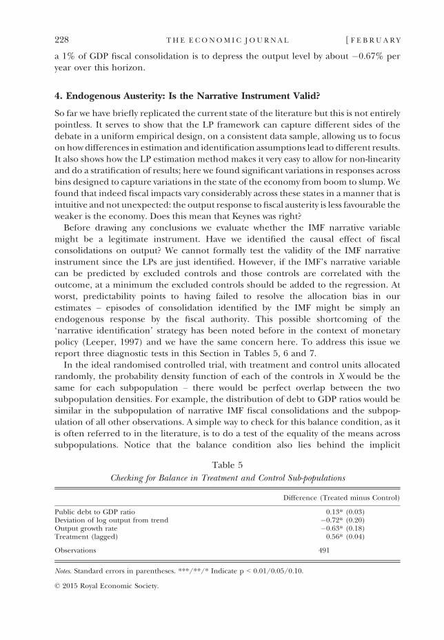
In the ideal randomised controlled trial, with treatment and control units allocatedrandomly, the probability density function of each of the controls in X would be thesame for each subpopulation – there would be perfect overlap between the twosubpopulation densities. For example, the distribution of debt to GDP ratios would besimilar in the subpopulation of narrative IMF fiscal consolidations and the subpop-ulation of all other observations. A simple way to check for this balance condition, as itis often referred to in the literature, is to do a test of the equality of the means acrosssubpopulations. Notice that the balance condition also lies behind the implicit

Table 5

Checking for Balance in Treatment and Control Sub-populations

Difference (Treated minus Control)

Public debt to GDP ratio 0.13* (0.03)Deviation of log output from trend �0.72* (0.20)Output growth rate �0.63* (0.18)Treatment (lagged) 0.56* (0.04)

Observations 491

Notes. Standard errors in parentheses. ***/**/* Indicate p < 0.01/0.05/0.10.



assumption that one can estimate the LP by restricting the coefficient of the controls tobe the same for the treatment and control groups, an observation that we discuss indetail in Section 5. The balance condition is evaluated in Table 5 for several potentiallyimportant macroeconomic control variables included in expression (1). The nullhypothesis of balance is rejected for all of them, strongly suggesting that the IMFnarrative dates are not truly exogenous events.

We go beyond this simple check and perform two additional tests. First, we check ifthe outcome is predictable by a set of available controls not yet included in the analysis.To be clear, the original AA and GLP papers do include in their analysis a robustnesscheck that includes other controls. However, the controls they consider are typicallyrelated fiscal variables rather than the set of macroeconomic controls we consider here.

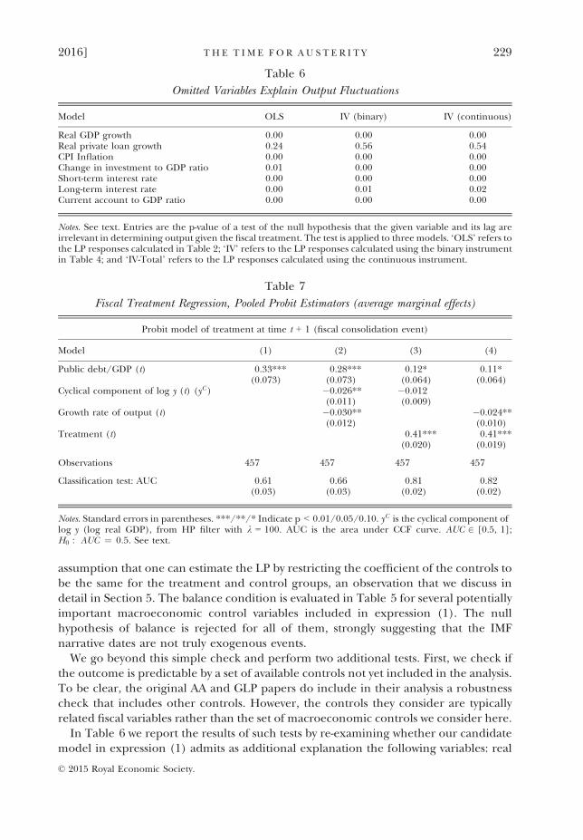
In Table 6 we report the results of such tests by re-examining whether our candidatemodel in expression (1) admits as additional explanation the following variables: real

Table 7

Fiscal Treatment Regression, Pooled Probit Estimators (average marginal effects)

Probit model of treatment at time t + 1 (fiscal consolidation event)

Model (1) (2) (3) (4)

Public debt/GDP (t) 0.33*** 0.28*** 0.12* 0.11*(0.073) (0.073) (0.064) (0.064)

Cyclical component of log y (t) (yC ) �0.026** �0.012(0.011) (0.009)

Growth rate of output (t) �0.030** �0.024**(0.012) (0.010)

Treatment (t) 0.41*** 0.41***(0.020) (0.019)

Observations 457 457 457 457

Classification test: AUC 0.61 0.66 0.81 0.82(0.03) (0.03) (0.02) (0.02)

Notes. Standard errors in parentheses. ***/**/* Indicate p < 0.01/0.05/0.10. yC is the cyclical component oflog y (log real GDP), from HP filter with k = 100. AUC is the area under CCF curve. AUC 2 [0.5, 1];H0 : AUC ¼ 0:5. See text.

Table 6

Omitted Variables Explain Output Fluctuations

Model OLS IV (binary) IV (continuous)

Real GDP growth 0.00 0.00 0.00Real private loan growth 0.24 0.56 0.54CPI Inflation 0.00 0.00 0.00Change in investment to GDP ratio 0.01 0.00 0.00Short-term interest rate 0.00 0.00 0.00Long-term interest rate 0.00 0.01 0.02Current account to GDP ratio 0.00 0.00 0.00

Notes. See text. Entries are the p-value of a test of the null hypothesis that the given variable and its lag areirrelevant in determining output given the fiscal treatment. The test is applied to three models. ‘OLS’ refers tothe LP responses calculated in Table 2; ‘IV’ refers to the LP responses calculated using the binary instrumentin Table 4; and ‘IV-Total’ refers to the LP responses calculated using the continuous instrument.



GDPgrowth; real private loan growth; CPI inflation; the change in the investment toGDPratio; the short-term interest rate on government securities (usually three-months inmaturity); the long-term rate on government securities (usually 5–10 year bonds); andthe current account to GDP ratio. The first three variables are expressed as 100 times thelog difference. In all cases, we consider the value of the variable and one lag. The tests areconducted with the one-period ahead local projection (the equivalent of thecorresponding equation in a VAR) using the full sample according to expression (1).

The objective is to set a higher bar for the possibly omitted regressors to be significant.Partitioning the sample into the growth bins we used earlier could generate spuriousfindings since the tests would rely on a smaller sample. Table 6 reports the p-valueassociated with the joint null that the candidate variable and its lag are not significant. Arejection means that output fluctuations could be due to reasons other than the fiscaltreatment variable. The message is clear: most of the excluded controls are highlysignificant. For now, a cautious interpretation is to view these findings as a source ofconcern rather thanconclusive evidence that themultipliers reportedearlier are incorrect.

Next we check for another condition: do excluded controls predict fiscal consol-idations? Table 7 asks whether variation in the IMF binary treatment variable identifiedby GLP can be predicted. The results indicate that we have a reasonable basis for thisconcern. This is a set of estimated treatment equations, where we use a pooled probitestimator to predict the IMF fiscal consolidation variable in year 1, presumptivelyannounced at year 0, based on state variables at time 0. As shown in the Appendix, ourlater results are robust to alternative binary classification models such as pooled logit,and fixed-effects probit and logit with controls for global time-varying trends.

Table 7 shows in column (1) that treatment is more likely, as expected, when publicdebt to GDP is high: the coefficient is positive, meaning that governments tend topursue austerity when debt has run up. In column (2) we add yC (the output gap) andthe growth rate of y to further condition on the state of the economy: when theeconomy is growing below potential, there is an increase in the likelihood ofconsolidation. Moreover, austerity is more likely to be pursued when growth slows, instark contrast to what common-sense textbook countercyclical policy suggests. But thisfinding is in line with contemporary experience in Europe and the UK, although all ofthe sample data we use here are pre-crisis. Thus, the act of engaging in pro-cyclicalfiscal policy is not a new-fangled craze but more of a chronic tendency in advancedcountries. Finally, columns (3) and (4) add the lag of the dependent variableTreatment and this has a highly significant coefficient: as we know from the raw dataseries generated by the IMF study, the fiscal consolidation episodes are typically long,drawn-out affairs, so once such a programme is started it tends to run for several years.Being in treatment today is thus a good predictor of being in treatment tomorrow. Inthese last two columns the lagged growth rate rather than the cyclical level of outputemerges as the slightly better predictor of treatment.

Further confirmation of the predictive ability of these treatment regressions isprovided by the AUC statistic.7 The AUC is commonly used in biostatistics and machinelearning to evaluate classification ability (Jord�a and Taylor, 2011). Under the null that

7 AUC stands for area under the curve. The curve usually refers to the Receiver Operating Characteristiccurve or ROC curve. It also refers to the Correct Classification Frontier, as in Jord�a and Taylor (2011).



the covariates have no classification ability, AUC = 0.5. Perfect classification abilitycorresponds to AUC = 1. The AUC has an approximate Gaussian distribution in largesamples. Table 7 measures the classification ability of each specification. The AUCstatistics show that the probits have very good predictive ability, with AUC around 0.65when lagged treatment is omitted (Column 2), and over 0.8 when lagged treatment isincluded (Columns (3) and (4)). The AUCs are all significantly different from 0.5.

The key lesson from Table 7 is simply that the IMF variable has a significantforecastable component.8 The question, then, is how to deal with the problem ofpotentially endogenous instruments. The remainder of this article provides one answer.

5. Statistical Design

The previous Section raises concerns that the narrative IMF variable could be aninvalid instrument using three different checks. The empirical strategy that we proposeis based on taking triple insurance against this potential endogeneity. First, we take theepisodes of consolidation from the IMF narrative variable as the subset of allconsolidation episodes that are a candidate for random allocation. Think of it as apseudo-IV step. Second, we include the extended set of covariates from Tables 6 and 7and add them as right hand side variables in the LP of expression (1). Third, we useinverse propensity score weighting on this LP to re-randomise allocation of the IMFfiscal consolidation events.

In order to facilitate the exposition we momentarily drop the cross-sectional countryindex in the panel. Denote, as before, yt the outcome variable of interest, the log ofreal GDP. In other applications yt could be a ky -dimensional vector. Let Dt denote thefiscal policy variable. Dt will now be a discrete random variable Dt 2 f0; 1g based on theIMF narrative indicator of exogenous fiscal consolidations, although earlier it was thecontinuous d.CAPB variable. The methods that we present next can be extended tosettings in which the policy variable takes on a small number of discrete values. Next weallow for a kw -dimensional vector of variables, wt that are not included in the vector yt ;but which could be relevant predictors of the policy variable Dt . Finally, denote Xt therich conditioning set given by Dyt�1; Dyt�2; . . .; Dt�1; Dt�2; . . .; and wt .

We assume that policy is determined by Dt ¼ DðXt ;w; etÞ where w refers to theparameters of the implied policy function and et is an idiosyncratic source of randomvariation. Therefore, DðXt ;w; :Þ refers to the systematic component of policy determi-nation.

To make further progress at this point, we will borrow from definition 1 in Angristet al. (2013, henceforth AJK). This defines potential outcomes given by ywt;hðdÞ � yt as

8 Hern�andez de Cos and Moral-Benito (2013) have arrived at a similar conclusion. Their proposedsolution to the lack of exogeneity problem is to use an instrumental variable approach. Instruments rely ondata for predetermined controls and on past consolidations. Since data on predetermined controls alreadyappear in the specification of previous studies (AA, GLP, etc.), the key question is whether past consolidationdata predict current consolidation episodes. Fixed-effect panel estimation already takes into accountheterogeneity in the unconditional probability of consolidation across countries. Take Australia as anexample, it is unlikely that the consolidation observed in 1985 helps determine the likelihood ofconsolidation in the year 1994 beyond the observation that Australia may consolidate more or less often thanthe typical country (already captured by the fixed effect). There may be little gained from the point of view ofstrengthening the identification.



the value that the observed outcome variable ytþh � yt would have taken if Dt ¼ d forall w 2 Ψ and d 2 D. In our application, the difference ytþh � yt refers to thecumulative change in the outcome from t to t + h and d = 0,1. The horizon h can beany positive integer.

The causal effect of a policy intervention is defined as the unobservable randomvariable given by the difference ½yt;hð1Þ � yt � � ½yt;hð0Þ � yt �: Notice that yt is only usedto benchmark the cumulative change and it is observed at time t. We assume that theparameters of the policy function do not change.

Following AJK, we can state the selection-on-observables assumption (or theconditional ignorability or conditional independence assumption as it is sometimescalled) as:

½ywt;hðdÞ � yt � ?Dt jXt ;w for all h[ 0; and for d 2 D and w 2 W: (2)

That is, the treatment-control allocation is independent of potential outcomes, giventhe variables or controls Xt . This condition does not imply that there is no effect of policyon the outcome given controls. We are simply stating that conditional on controls, policyallocation is independent of the potential outcome, whatever that might be.

Consider the ideal randomised experiment to understand the role that theconditional independence assumption plays. The average causal effect of policyintervention on the outcome at time t + h given by:

Ef½yt;hð1Þ � yt � � ½yt;hð0Þ � yt �g;could be simply calculated using group means as:

KhGroupMean ¼ 1

n1

Xt

Dtðytþh � ytÞ � 1

n0

Xt

ð1� DtÞðytþh � ytÞ for all h[ 0; (3)

where n1 ¼ Rt Dt and n0 ¼ Rtð1 � DtÞ are the number of observations in treatmentand control groups, respectively.

Alternatively, the ATE, Kh , could be calculated from the auxiliary regression:

ðytþh � ytÞ ¼ Dtah1 þ ð1� DtÞah0 þ vtþh for all h[ 0: (4)

The difference in the OLS estimates of the intercepts ah1 � ah0 ¼ Kh in expression(4) is equivalent to that in expression (3). More conveniently, one could estimate theATE directly from the regression:

ðytþh � ytÞ ¼ ah0 þ DtKh þ vtþh for all h[ 0: (5)

Even when data are randomly allocated across the treatment and control subpopu-lations, it would be natural to condition on the Xt to adjust for small-sample differencesin subpopulation characteristics and therefore to gain in efficiency. The estimator isconsistent for the ATE whether or not regressors are included. Notice that themodel forthe outcomes is unspecified. The estimate of the ATE does not depend on specificassumptions about this model if the conditional ignobility assumption is met.

Allocation to treatment and control groups is not usually random in observationaldata. To appreciate the role of the selection-on-observables assumption in (2),consider elaborating on the example. First, by the law of iterated expectations, we canwrite:



Ef½yt;hð1Þ� yt � � ½yt;hð0Þ� yt �g ¼ E½Eðytþh � yt jDt ¼ 1;XtÞ�Eðytþh � yt jDt ¼ 0;XtÞ�¼Kh for all h[0: (6)

Assume that a linear regression control strategy suffices to do the appropriateconditioning for the Xt and hence obtain a consistent estimate of E½ytþh � yt jDt ;Xt �.This is a big assumption that we relax later on in the article. Note this is the assumptionof studies based on VARs where identification does not rely on external information.Then the average causal effect of a policy intervention on the outcome variable at timet+h in the maintained example, can be calculated by expanding expression (4) with

ytþh � yt ¼ Dtah1 þ ð1� DtÞah0 þ DtXtb

h1 þ ð1� DtÞXtb

h0 þ vtþh for all h[ 0: (7)

If one imposes the constraint bh1 ¼ bh0, then expression (7) is nothing more than astandard LP of expression (1) andKh ¼ ah1 � ah0 is the policy response at horizon h. Thestandard linear LP is a direct estimate of the typical impulse response derived from atraditional VAR, as Jord�a (2005) shows. This na€ıve constrained specification, whichcharacterises responses derived from a VAR, imposes two implicit assumptions. First, theeffect of the controls Xt on the outcomes is assumed to be stable across the treated andcontrol subpopulations. Second, the expected value of Xt in each subpopulation isassumed to be the same. The first assumption is potentially defensible. The economicmechanism describing the transmission of interest rates on real GDP could be the samewhether or not there is a fiscal consolidation, for example. The second assumption ismore difficult to defend. It is unlikely that, say, government debt levels are the same in thetreated and control groups. Fiscal consolidations are often driven by high levels of debt.

This is a good place to make a connection with structural VAR identification. Whenh = 1, the LP is equivalent to the corresponding equation in a VAR. A specification thatincludes all contemporaneous variables as controls (in addition to their lags) could beseen as equivalent to imposing the Choleski ordering in which the policy variable isordered last. However, unlike a VAR, there is no need to impose exclusion restrictionson the remaining variables in the system if the focus shifts to a different response/intervention pair. Practically speaking it would be advisable not to impose suchconstraints but rather include all available observable controls again and let the datachoose which variables are appropriate conditioning information. The larger principleis to ensure that fluctuations in the shocked variable cannot be explained by anyobservable information. In that respect, it is perhaps useful to remember that the truesquare-root of the reduced-form residual covariance matrix need not be upper-triangular or even have any zero entries for that matter.

When instruments are available one can further achieve identification usinginstrumental variable methods as in Stock and Watson (2012) and Mertens and Ravn(2013, 2014). We have shown above how IV methods can be used with the LP approachin a more natural way. However, it is important to recall several features required toresolve the identification puzzle. These are:

(i) the instrument is relevant, which appears to be the case as we discussed earlier;(ii) the instrument is valid, which is untestable given just-identification and for

which the analysis of the previous Section raises concerns; and



(iii) predetermined and exogenous controls are not omitted from the specifica-tion.

This latter requirement is not resolved by the use of the instrument, especially whenthere is substantial evidence that the controls are predictive for the instrument, asshown here.

Taking up our earlier discussion once more, using expressions (6) and (7), noticethat:

EðEf½yt;hð1Þ � yt � � ½yt;hð0Þ � yt �jXtgÞ¼ E E ½Dtða1 þ Xt b

h1Þ� � ½ð1� DtÞða0 þ Xt b

h0Þ�jXt

n o� �¼ Eðah1 � ah0Þ¼ EðKhÞ ¼ Kh;

under the maintained assumptions of the example that EðXt jDt ¼ 1Þ ¼ EðXt jDt ¼ 0Þand b1 ¼ b0 and noticing that EðDt jDt ¼ 1Þ ¼ E½ð1� DtÞjDt ¼ 0� ¼ 1.

More generally, if we do not impose the implicit assumptions of the na€ıve LPspecification, the analogous representation to the group means expression (3) is:

KhRA ¼ 1

n1

Xt

Dt ½mh1 ðX t ; h

h1Þ� �

1

n0

Xt

ð1� DtÞ½mh0ðX t ; h

h0Þ� for all h[ 0; (8)

where mhj ð:Þ is a generic specification of the conditional mean of ðytþh � ytÞ in each

subpopulation j = 1,0 and hhj ¼ ðahj bhj Þ0for the regression example in (7). The n1

and n0 have been defined earlier. Note that this more general form of regressionadjustment allows the conditional means to be different for the treated and controlsubpopulations and allows their effect on the outcome to differ as well.

5.1. Re-randomisation Through the Propensity Score

Recall that the critical assumption is the conditional ignorability or selection-on-observables condition (2). Rosenbaum and Rubin (1983) show that:

Xt ?Dt jpðDt ¼ 1jXt ;wÞ;that is, the propensity score pðDt ¼ 1jXt ;wÞ is all that is needed to capture the effect ofthe Xt in the selection-on-observables condition.9 This result provides further supportfor the IPW estimator. Recall the ATE is, by definition:

Kh ¼ Ef½yt;hð1Þ � yt � � ½yt;hð0Þ � yt �g ¼ EðEf½yt;hð1Þ � yt � � ½yt;hð0Þ � yt �jXtgÞ; (9)

using the law of iterated expectations. Looking inside the expectations in the final termabove, the average policy response conditional on Xt , in terms of observable data, is:

9 Correction of incidental truncation with IPW has a long history in statistics (Horvitz and Thompson,1952) and is generally viewed as more general than Heckman’s (1976) selection model. Heckman’s (1976)approach corrects for incidental truncation using the inverse Mills ratio, requires specific distributionalassumptions, and at least one selection variable not affecting the structural equation. Heckman’s approach isonly known to work for special non-linear models, such as an exponential regression model (Wooldridge,1997). See Wooldridge (2010) for a more general discussion.



Ef½yt;hð1Þ � yt � � ½yt;hð0Þ � yt �jXtg¼ E½yt;h � yt jDt ¼ 1;Xt � � E½yt;h � yt jDt ¼ 0;Xt �; for all h[ 0; (10)

where it is assumed that the policy environment characterised by w 2 Ψ remainsconstant. Estimation of these conditional expectations can be simplified considerablywhen a model for the policy variable Dt is available.

Angrist and Kuersteiner (2004, 2011) refer to the predicted value from such apolicy model as the policy propensity score. The policy propensity score is meant toensure the estimation of the policy response (the ATE in the microeconomicsparlance) is consistent under the main assumption. In addition, it acts as adimension-reduction device. Ideally, any predictor of policy should be included,regardless of whether that predictor is a fundamental variable in a macroeconomicmodel. The probit results reported in Table 7 can be seen as candidate estimatesof this policy propensity score. We instead construct the policy propensityscore using a richer specification that includes all the controls used in Table 6 aswell.

Denote the policy propensity score PðDt ¼ j jXtÞ ¼ pjðXt ;wÞ for j = 1,0. Clearlyp1ðXt ;wÞ ¼ 1 � p0ðXt ;wÞ. Using the selection-on-observables condition in expression(2) shown earlier, then:

E½ðyt;h � ytÞ1fDt ¼ jgjXt � ¼ Ef½yt;hðjÞ � yt �jXtgpjðXt ;wÞ for j ¼ 1; 0: (11)

Solving for Ef½yt;hðjÞ � yt �jXtg and taking unconditional expectations, by integratingover Xt , the ATE in (9) can be calculated as:

Kh ¼ Ef½yt;hð1Þ � yt � � ½yt;hð0Þ � yt �g

¼ E ðyt;h � ytÞ 1fDt ¼ 1gp1ðXt ;wÞ � 1fDt ¼ 0g

p0ðXt ;wÞ� ��

for all h[ 0:(12)

Under standard regularity conditions (detailed in AJK) an estimate of expression (12)can be obtained using sample moments which generalise the sample momentspresented earlier in expression (3) for the OLS case.

Suppose that the first-stage treatment model takes the form of a probability oftreatment at time t given by the estimated model pt ¼ p1ðX t ; wÞ, where w is theestimated parameter vector, and 1 � pt ¼ p0ðX t ; wÞ. The inverse propensity scoreweighted (IPW) ‘ratio estimator’ of the ATE is:

KIPW ¼ 1

n

Xt

Dtðytþh � ytÞpt

� �� 1

n

Xt

ð1� DtÞðytþh � ytÞ1� pt

� �: (13)

Some improvements can be made to this expression. Imbens (2004) and Luncefordand Davidian (2004) suggest renormalising the weights so that they sum up to one insmall samples. Hence expression (13) becomes:

KIPW ¼ 1

n�1

Xt


� �� 1

n�0

Xt

ð1� DtÞðytþh � ytÞ1� pt

� �; (14)



where

n�1 ¼

Xt

Dt

pt

!n�0 ¼

Xt

ð1� DtÞð1� ptÞ

" #; (15)

and the notation n�j parallels the notation nj for j = 1,0 in (3). Note that

EðDt=ptÞ ¼ E½EðDt jXtÞ�=pt ¼ 1; similarly E½ð1 � DtÞ=ð1 � ptÞ� ¼ EfE½ð1 � DtÞjXt �g=ð1 � ptÞ ¼ 1; and hence it follows that in large samples expressions (13) and (14)apply the same weighting, since Eðn�

1Þ ¼ Eðn�0Þ ¼ n. These expressions are natural

analogs of the Group Mean estimator in (3), with inverse propensity-score weighting tocorrect for allocation bias and to achieve a quasi-random distribution of treatment andcontrol observations via reweighting.

5.2. Regression Adjustment (IPWRA) and Augmented IPW (AIPW)

As a way to enhance robustness, researchers have derived estimators with a regressionadjustment component added to the standard IPW estimator presented above. Thisestimator parallels that in expression (8) but using IPW. To further enhance efficiency,the augmented IPW or AIPW estimator combines the IPW and IPWRA estimators in amanner to be discussed shortly.

It is natural to consider extending the estimator in expression (8) using thepropensity score. Formally, the basis for such an estimator would be to transition fromexpression (11) to (12) in the following manner:

Kh ¼ E ðytþh � yt jXtÞ 1fDt ¼ 1gp1ðXt ;wÞ � 1fDt ¼ 0g

p0ðXt ;wÞ� ��

for all h[ 0; (16)

which can be implemented by first projecting the outcome variable on the set ofcontrol variables (Robins and Rotnitzky, 1995; Robins et al., 1995; Wooldridge, 2007).The inverse propensity score weighted estimator with regression adjustment (IPWRA)is then given by:

KhIPWRA ¼ 1

n�1

X Dtmh1ðX t ; h1

hÞpt

" #� 1

n�0

X ð1� DtÞmh0ðX t ; h0

hÞ1� pt

" #; (17)

where again mhj ðX t ; hj

hÞ for j = 1,0 is the conditional mean from the first-stepregression of ðytþh � ytÞ on Xt as in expression (8) in Section 5. The n�

j for j = 1,0 arethe same as in expression (15). It is clear that (17) nests all the previous estimators, theGroup Mean (3), the RA (8) and the IPW (14) as special cases.

The estimator in expression (17) falls into the class of doubly robust estimators(Imbens, 2004; Lunceford andDavidian, 2004;Wooldridge, 2007; Kreif et al., 2013). Theintuition behind the estimator is to use the regression model as a way to ‘predict’ theunobserved potential outcomes. Consistency of the estimated ATE only requires eitherthe conditional mean model or the propensity score model to be correctly specified.

However, although (17) is one of a large class of unbiased IPWRA estimators of ATE,it is not the most efficient in this class. Starting with Robins et al. (1994) and morerecently, Lunceford and Davidian (2004), the estimator within the doubly-robust classhaving the smallest asymptotic variance, is the (locally) semi-parametric efficient



estimator:

KhAIPW ¼ 1

n

Xt


� ð1� DtÞðytþh � ytÞð1� ptÞ

� ��

� ðDt � ptÞptð1� ptÞ

ð1� ptÞmh1ðXt ; h

h1Þ þ ptm

h0 ðXt ; h

h0Þ

h i�: (18)

Thus, the estimator in (18) can be seen as the basic IPW estimator plus anadjustment consisting of the weighted average of the two regression estimators. Theadjustment term has expectation zero when the estimated propensity scores andregression models are replaced by their population counterparts. Moreover, theadjustment term stabilises the estimator when the propensity scores get close to zero orone (Glynn and Quinn, 2010) and this alleviates the need to truncate the propensityscore weights as suggested in Imbens (2004). Another way to interpret the AIPWestimator is to realise that:

KhAIPW ¼ Kh

IPW þ ðKhRA � Kh

IPWRAÞ: (19)

Readers familiar with the bootstrap will notice the similarities between the bootstrapbias correction formula and (19).

The AIPW has a number of attractive theoretical properties. Using the theory of M-estimation, Lunceford and Davidian (2004) show that the estimator is asymptoticallynormally distributed. In addition, they show that the variance can be calculated usingthe empirical sandwich estimator V ðKh

AIPW Þ ¼ 1n2

PtðI ht Þ2, where:

I ht ¼ Dtðytþh � ytÞpt

� ð1� DtÞðytþh � ytÞð1� ptÞ

� ��

� ðDt � ptÞptð1� ptÞ

ð1� ptÞmh1ðXt ; h

h1Þ þ ptm

h0 ðXt ; h

h0Þ

h i�� Kh

AIPW :

(20)

Later we allow for the possibility that the I ht are not a martingale difference sequenceand calculate standard errors using cluster robust methods. When the propensity scoreand the regression function are modelled correctly, the AIPW achieves the semi-parametric efficiency bound. Alternatively, Imbens (2004) shows that standard errorsfor Kh

AIPW can be calculated with the bootstrap.

5.3. Intuition

Although these techniques are relatively new to macroeconomics, matchingestimators using inverse propensity score weighting have been frequently implemen-ted in applied microeconomics with cross-sectional data. Matching methods moregenerally constitute a benchmark within the medical research literature when trialsare suspected of being contaminated by allocation bias. The provenance of theparticular inverse propensity score weighting method we employ is thus wellestablished.

Figure 1 provides intuition for the methods that we just described and exemplifiesthe perils of allocation bias with a simple bivariate manufactured example based oneobservable confounder. Panel (a) displays the hypothetical frequencies of observing



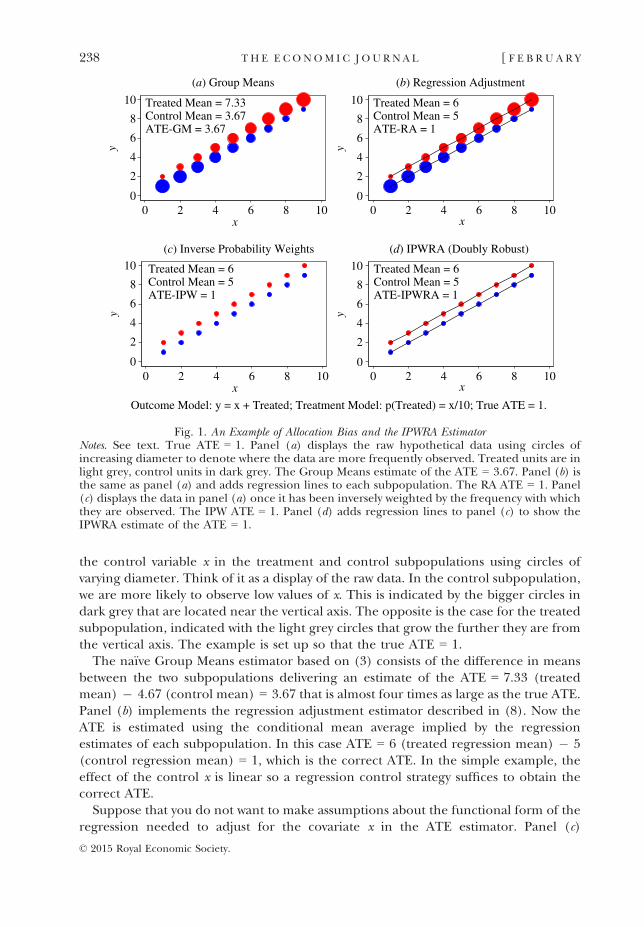
the control variable x in the treatment and control subpopulations using circles ofvarying diameter. Think of it as a display of the raw data. In the control subpopulation,we are more likely to observe low values of x. This is indicated by the bigger circles indark grey that are located near the vertical axis. The opposite is the case for the treatedsubpopulation, indicated with the light grey circles that grow the further they are fromthe vertical axis. The example is set up so that the true ATE = 1.

The na€ıve Group Means estimator based on (3) consists of the difference in meansbetween the two subpopulations delivering an estimate of the ATE = 7.33 (treatedmean) � 4.67 (control mean) = 3.67 that is almost four times as large as the true ATE.Panel (b) implements the regression adjustment estimator described in (8). Now theATE is estimated using the conditional mean average implied by the regressionestimates of each subpopulation. In this case ATE = 6 (treated regression mean) � 5(control regression mean) = 1, which is the correct ATE. In the simple example, theeffect of the control x is linear so a regression control strategy suffices to obtain thecorrect ATE.

Suppose that you do not want to make assumptions about the functional form of theregression needed to adjust for the covariate x in the ATE estimator. Panel (c)

Treated Mean = 7.33Control Mean = 3.67ATE-GM = 3.67

0

2

4

6

8

10y

0

2

4

6

8

10

y

0

2

4

6

8

10

y

0

2

4

6

8

10

y

0 2 4 6 8 10x

(a) Group Means

Treated Mean = 6Control Mean = 5ATE-RA = 1

0 2 4 6 8 10x

(b) Regression Adjustment

Treated Mean = 6Control Mean = 5ATE-IPW = 1

0 2 4 6 8 10x

(c) Inverse Probability Weights

Treated Mean = 6Control Mean = 5ATE-IPWRA = 1

0 2 4 6 8 10x

(d) IPWRA (Doubly Robust)

Outcome Model: y = x + Treated; Treatment Model: p(Treated) = x/10; True ATE = 1.

Fig. 1. An Example of Allocation Bias and the IPWRA EstimatorNotes. See text. True ATE = 1. Panel (a) displays the raw hypothetical data using circles ofincreasing diameter to denote where the data are more frequently observed. Treated units are inlight grey, control units in dark grey. The Group Means estimate of the ATE = 3.67. Panel (b) isthe same as panel (a) and adds regression lines to each subpopulation. The RA ATE = 1. Panel(c) displays the data in panel (a) once it has been inversely weighted by the frequency with whichthey are observed. The IPW ATE = 1. Panel (d) adds regression lines to panel (c) to show theIPWRA estimate of the ATE = 1.



implements the IPW estimator in (17). Using weights based on the inverse frequencywith which the data are observed for each value of x in each subpopulation generates a‘pseudo-randomised’ sample from which the simple difference in mean estimatordelivers the correct answer. In this case ATE = 6 (treatment mean using inverseweights) � 5 (control mean using inverse weights) = 1, again the correct value.

In practice, one may be unsure about the correct specification of either theregression or the propensity score describing the appropriate reweighing scheme.Panel (d) combines the two approaches (IPW and regression adjustment) based onexpression (17). This estimator is ‘doubly robust’ meaning that either the propensityscore or the regression may be incorrectly specified and yet still deliver the correctestimate of the ATE. In the example there is no gain from using this procedure butone can still verify that ATE = 6 (conditional regression mean for treated using inverseweighting) � 5 (conditional regression mean for control using inverse weighting) = 1.Again, the correct ATE.

When policy interventions are mostly driven by the endogenous response to controls,we can think of the observable treatment/control subpopulations as being oversampledfrom the regionof thedistribution inwhich thepropensity score attains its highest values.Moments calculated with this raw empirical distribution will therefore be biased: notenoughprobabilitymass is given to observations with lowpropensity scores.Weighting bythe inverse of the propensity score shifts weight away from the oversampled toward theundersampled region of the distribution. This shift of probability mass reconstructs theappropriate frequency weights of the underlying true distribution of outcomes undertreatment and control so that the means estimated from each subpopulation are nolonger biased and their difference is an unbiased estimate of the ATE.

5.4. What We Do

The next Section reports the results of applying the AIPW estimator (18) to measurethe ATE of fiscal consolidations as a counterpoint to the conventional OLS and IVresults reported earlier. As a way to understand where the differences come from, wefirst implement the AIPW estimator by restricting the parameters of the regression(based on LPs) to be the same in the treated and control subpopulations, as is implicitin the OLS and IV approaches. Under that constraint, the results from the AIPWestimator are close to the IV results seen earlier. Next we allow for the parameters tovary across subpopulations, adhering to the way expression (18) is typically applied inthe policy evaluation literature. These results deliver the same qualitative implicationof contractionary austerity but show that the effects of consolidations are quantitativelyeven more painful.

6. Contractionary Austerity Revisited: Estimates of the Average Effect of FiscalConsolidations

This Section presents AIPW estimates of the ATE of fiscal consolidations. Followingstandard procedures, the propensity score used here is based on a saturated probitmodel that extends the set of controls used in Table 7 with the current and laggedvalues of the controls in Table 6. The saturated probit also includes country fixed



effects. Although we do not report the coefficient estimates of this more saturatedmodel, it is worth mentioning that the AUC in this treatment model rises to 0.86.

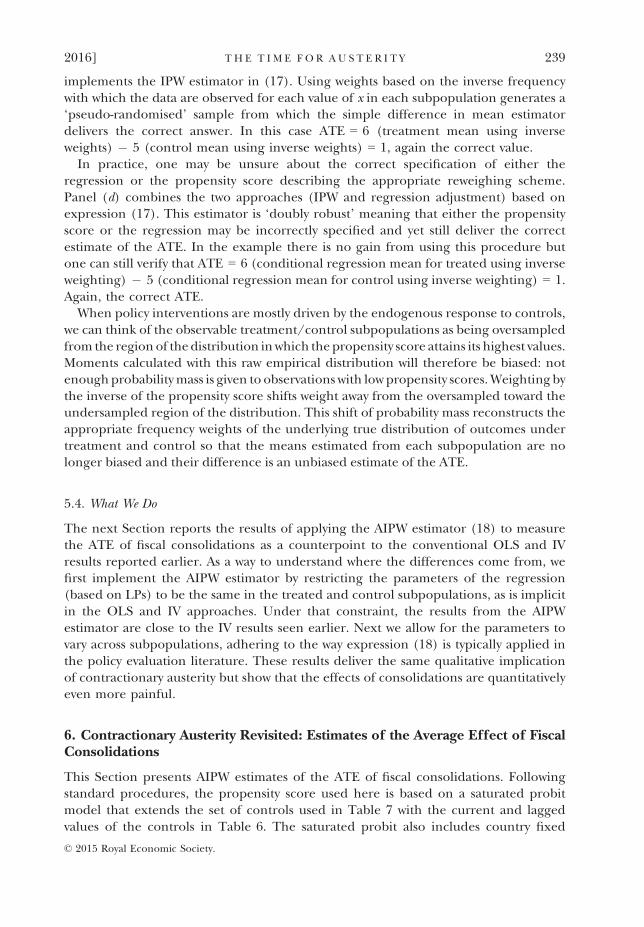
Figure 2 provides smooth kernel density estimates of the distribution of thepropensity score for the treated and control units to check for overlap. One way tothink of overlap is to consider what overlap would be in the ideal RCT. The empiricaldistributions of the propensity score for treated and control units would be uniformand identical to each other. At the other extreme, suppose that treatment is allocatedmechanically on the basis of controls. Then the distribution of treated units wouldspike at one and be zero elsewhere and the distribution of control units would spike atzero and be zero elsewhere. Despite the high AUC, the Figure indicates considerableoverlap between the distributions, which indicates we have a satisfactory first-stagemodel with which to identify the ATE properly using IPW methods.

However, the Figure also indicates that there are some observations likely to get veryhigh weights. Specifically, there are control (treated) units whose propensity score isnear zero (one) and hence who get weights in the IPW in excess of 10. In general, it isoften recommended to truncate the maximum weights in the IPW to 10 (Imbens,2004; Cole and Hern�an, 2008). However, the AIPW has the property that high weightsin the IPW are compensated at the same rate by the augmentation term. Experimentsnot reported here indicate that this is indeed what happens in practice and thattruncation is unnecessary in our application (see Appendix A.3).

Using the more saturated probit, we then estimate cumulated responses and theirsum to the five-year horizon as before. Our indicator of a fiscal consolidation is thenarrative IMF indicator, the Treatment variable. Since Treatment is binary, we areestimating average effects only. However, coincidentally, the average treatment size (or

Distribution for Control Units

Distribution for Treated Units

0

1

2

3

4

Freq

uenc

y

0 1Estimated Probability of Treatment

Fig. 2. Overlap Check: Empirical Distributions of the Treatment Propensity ScoreNotes. See text. The propensity score is estimated using the saturated probit specificationdiscussed in the text, which includes country fixed effects. The Figure displays the predictedprobabilities of treatment with a dashed line for the treatment observations and with a solid linefor the control observations.



dose) is close to 1% of GDP in these data (the exact value is 0.97, with a standarddeviation of 0.07 in the full sample and is not significantly different in booms andslumps), so the interpretation of these responses is directly comparable to aconventional multiplier, with only a small upscaling (of 1/0.97) for strict accuracy.We can return to this rescaling issue in a moment when we make a formal comparisonwith the previous OLS and IV results.

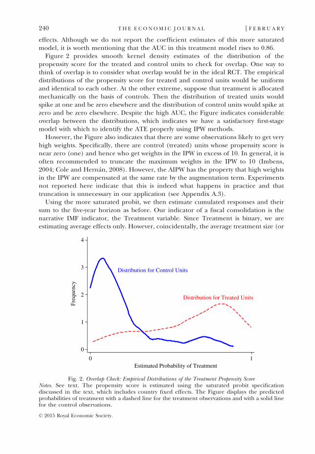
We begin by discussing Table 8, which is the direct counterpart to the OLS and IVresult presentations in Tables 1 and 3. Here we show the ATE of fiscal consolidationusing the AIPW estimator (18), for the full sample (i.e. no use of boom and slump bins,yet) and using the propensity score estimates based on the saturated probit. Both thetreatment equation probit model and the outcome-equation AIPW model includecountry-fixed effects.

Table 8 is organised into two rows. The first row reports the results based onimposing the restriction hh1 ¼ hh0, the usual implicit restriction used without hesitationin the macro-VAR empirical literature and is the same restriction we imposed inreporting the results of Tables 1 and 3. The second row reports the results that do notimpose the hh1 ¼ hh0 restriction. The results are qualitatively similar to those reported inTable 3 in that we still find that austerity is contractionary. However, the estimatedimpacts of fiscal consolidations on output are now even bigger.

Recall that according to the IV estimates, the accumulated loss over five years was�2:94��. This would imply an average annual real GDP loss of about 0.59% of GDP per1% of fiscal consolidation over each of the five years. Here our AIPW estimate withunrestricted coefficients has a sum effect of�3:61�� over five years. This would imply anaverage annual real GDP loss of about 0.74% of GDP per 1% of fiscal consolidation overeachof thefive years (using a 1/0.97 rescaling factor). Thus the implied output losses dueto austerity are about 20% larger under our AIPW estimation than with IV estimation.

Next we once again explore the same partition of the data into booms and slumps,allocating to the bins according to whether output is above or below trend as in earlier

Table 8

Average Treatment Effect of Fiscal Consolidation, AIPW Estimates, Full Sample

Deviations of log real GDP (relative to Year 0, 9 100)


Fiscal ATE, restricted (hh1 ¼ hh0) �0.17 �0.55** �0.61*** �0.88** �1.14** �3.22***(0.17) (0.23) (0.20) (0.32) (0.42) (0.89)

Fiscal ATE, unrestricted (hh1 6¼ hh0) �0.24 �0.70** �0.75*** �0.93** �1.23** �3.61***(0.16) (0.26) (0.25) (0.33) (0.47) (1.06)

Observations 456 439 423 406 389 389

Notes. Empirical sandwich standard errors (clustered by country) in parentheses (see expression (20)).***/**/* Indicate p < 0.01/0.05/0.10. Conditional mean controls: cyclical component of y, two lags ofchange in y, country fixed effects. yC is the cyclical component of log y (log real GDP), from HP filterwith k = 100. Specification includes country fixed effects in the propensity score model and in the AIPWmodel. Propensity score based on the saturated probit model as described in the text. AIPW estimates donot impose restrictions on the weights of the propensity score. Truncated results not reported here butavailable upon request. See text.



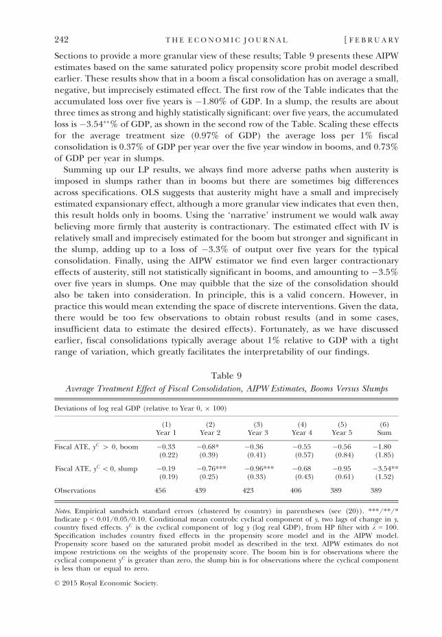
Sections to provide a more granular view of these results; Table 9 presents these AIPWestimates based on the same saturated policy propensity score probit model describedearlier. These results show that in a boom a fiscal consolidation has on average a small,negative, but imprecisely estimated effect. The first row of the Table indicates that theaccumulated loss over five years is �1.80% of GDP. In a slump, the results are aboutthree times as strong and highly statistically significant: over five years, the accumulatedloss is �3:54��% of GDP, as shown in the second row of the Table. Scaling these effectsfor the average treatment size (0.97% of GDP) the average loss per 1% fiscalconsolidation is 0.37% of GDP per year over the five year window in booms, and 0.73%of GDP per year in slumps.

Summing up our LP results, we always find more adverse paths when austerity isimposed in slumps rather than in booms but there are sometimes big differencesacross specifications. OLS suggests that austerity might have a small and impreciselyestimated expansionary effect, although a more granular view indicates that even then,this result holds only in booms. Using the ‘narrative’ instrument we would walk awaybelieving more firmly that austerity is contractionary. The estimated effect with IV isrelatively small and imprecisely estimated for the boom but stronger and significant inthe slump, adding up to a loss of �3.3% of output over five years for the typicalconsolidation. Finally, using the AIPW estimator we find even larger contractionaryeffects of austerity, still not statistically significant in booms, and amounting to �3.5%over five years in slumps. One may quibble that the size of the consolidation shouldalso be taken into consideration. In principle, this is a valid concern. However, inpractice this would mean extending the space of discrete interventions. Given the data,there would be too few observations to obtain robust results (and in some cases,insufficient data to estimate the desired effects). Fortunately, as we have discussedearlier, fiscal consolidations typically average about 1% relative to GDP with a tightrange of variation, which greatly facilitates the interpretability of our findings.

Table 9

Average Treatment Effect of Fiscal Consolidation, AIPW Estimates, Booms Versus Slumps

Deviations of log real GDP (relative to Year 0, 9 100)


Fiscal ATE, yC [ 0, boom �0.33 �0.68* �0.36 �0.55 �0.56 �1.80(0.22) (0.39) (0.41) (0.57) (0.84) (1.85)

Fiscal ATE, yC \ 0, slump �0.19 �0.76*** �0.96*** �0.68 �0.95 �3.54**(0.19) (0.25) (0.33) (0.43) (0.61) (1.52)

Observations 456 439 423 406 389 389

Notes. Empirical sandwich standard errors (clustered by country) in parentheses (see (20)). ***/**/*Indicate p < 0.01/0.05/0.10. Conditional mean controls: cyclical component of y, two lags of change in y,country fixed effects. yC is the cyclical component of log y (log real GDP), from HP filter with k = 100.Specification includes country fixed effects in the propensity score model and in the AIPW model.Propensity score based on the saturated probit model as described in the text. AIPW estimates do notimpose restrictions on the weights of the propensity score. The boom bin is for observations where thecyclical component yC is greater than zero, the slump bin is for observations where the cyclical componentis less than or equal to zero.



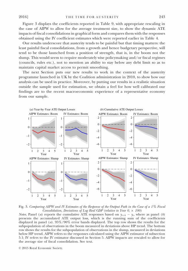
Figure 3 displays the coefficients reported in Table 9, with appropriate rescaling inthe case of AIPW to allow for the average treatment size, to show the dynamic ATEimpacts of fiscal consolidations in graphical form and compares themwith the responsesobtained using the IV coefficient estimates which were reported earlier in Table 4.

Our results underscore that austerity tends to be painful but that timing matters: theleast painful fiscal consolidations, from a growth and hence budgetary perspective, willtend to be those launched from a position of strength, that is, in the boom not theslump. This would seem to require moderately wise policymaking and/or fiscal regimes(councils, rules etc.), not to mention an ability to stay below any debt limit so as tomaintain capital market access to permit smoothing.

The next Section puts our new results to work in the context of the austerityprogramme launched in UK by the Coalition administration in 2010, to show how ouranalysis can be used in practice. Moreover, by putting our results in a realistic situationoutside the sample used for estimation, we obtain a feel for how well calibrated ourfindings are to the recent macroeconomic experience of a representative economyfrom our sample.

–2

–1

0

1

–2

–1

0

1

–2

–1

0

1

–2

–1

0

1

1 2 3 4 5Year

AIPW Estimates: Boom

1 2 3 4 5Year

IV Estimates: Boom

1 2 3 4 5Year

AIPW Estimates: Slump

1 2 3 4 5Year

IV Estimates: Slump

(a) Year-by-Year ATE Output Losses

–6

–4

–2

0

2

–6

–4

–2

0

2

–6

–4

–2

0

2

–6

–4

–2

0

2

1 2 3 4 5Year

AIPW Estimates: Boom

1 2 3 4 5Year

IV Estimates: Boom

1 2 3 4 5Year

AIPW Estimates: Slump

1 2 3 4 5Year

IV Estimates: Slump

(b) Cumulative ATE Output Losses

Fig. 3. Comparing AIPW and IV Estimates of the Response of the Output Path in the Case of a 1% FiscalConsolidation, Deviations of Log Real GDP (relative to Year 0, 9 100)

Notes. Panel (a) reports the cumulative ATE responses based on ytþh � yt , where as panel (b)presents the accumulated ATE output loss, which is the running sum of the coefficientsdisplayed in panel (a). 95%/90% error bands displayed. The top row shows the results for thesubpopulation of observations in the boom measured in deviations above HP trend. The bottomrow shows the results for the subpopulation of observations in the slump, measured in deviationsbelow HP trend. AIPW refers to the responses calculated using the AIPW estimator of subsection5.1; IV refers to the IV estimator discussed in Section 5. AIPW impacts are rescaled to allow forthe average size of fiscal consolidation. See text.



7. Counterfactual: Coalition Austerity and the UK Recession

This Section makes a counterfactual forecast of the post-2007 path of the UK economywithout the fiscal austerity policies imposed by the Coalition Government after the2010 election. These estimates are based on a sample that excludes the GlobalFinancial Crisis. Therefore, the exercise has the flavour of an out-of-sample evaluation.

We need to be very clear about the assumptions, explicit or implicit, in ourcounterfactual. We assume that zero fiscal consolidation was done in the years 2010–3 asthe counterfactual, that this was feasible, and would have not caused other possiblyadverse outcomes. Most crucially we assume that this would have had no damagingeffect on UK government debt yields, or country risk, in the relevant time frame. Weassume, in other words, that the UK had the fiscal space to follow a counterfactual pathfor those years. Critics may question this assumption but no evidence has been adducedto support their view. First, without a model on their part of the determinants of UKsovereign risk showing such a spike, the point is not well supported. In fact, to the extentthat we have any cross-country evidence on the impact of fiscal consolidations onsovereign yields it shows that austerity tends to worsen sovereign spreads, or has a smalland often non-significant efffect (Born et al., 2015, Figure 4). Second, the evidencefrom UK longer-run history is even less favourable: the country emerged from theNapoleonic Wars and the two World Wars with debt ratios higher than current levelsrelative to GDP (and tax revenues much lower) and yet never defaulted on market debtor lost capital market access. So there is no within-country evidence of this link either.Third, recent UK history also goes against this argument: despite public debt levelsrising under the Coalition (mainly because a slow recoverymeant poor tax revenues) theUK gilt yield has fallen to its lowest level in centuries. Indeed, with stronger outputgrowth under the counterfactual, tax revenues would have been higher, a factor thatwould have alleviated debt build up, all else equal.10

The UK experienced amuch weaker recovery than in the US, where nothing close to adouble dip took place. The divergence between the two recovery paths began in 2010(Schularick and Taylor, 2012). Since both countries’ central banks acted with aggressiveeasing, by going to the zero bound and pursuing quantitative easing policies thereafter,explanations for the differences have focused elsewhere. Various explanations havebeen offered, ranging from tighter UK fiscal policy, to spillovers from the Eurozone andweak trade links with fast-growth emerging markets. Other stories have invokedcontractions in oversized UK sectors such as finance and North Sea oil and gas, theextent of non-bank finance and differential energy costs (Davies, 2012; Posen, 2012).

To gain quantitative traction on the share of responsibility that should be borne byfiscal policy we use our AIPW estimates. We scale, and assign the impacts of fiscalshocks as follows. As a measure of the change in fiscal stance we use the change in the

10 Low yields have been evident throughout the advanced economies in recent years, outside the Eurozonecrisis countries. Though outside the scope of our article, the main explanations for these trends would seemto be a strong medium-run flight to safety since 2008 and a longer-run drift to lower real rates globally overtwo decades driven by global demography and/or EM precautionary saving motives. An additional factor isthat having its own central bank means that the UK cannot suffer a sudden stop or a self-fulfilling run on thesovereign like, say, countries in the Eurozone periphery. Together, these factors appear have contributed toenlarged fiscal space in the form of a massive absorption potential for UK gilts.



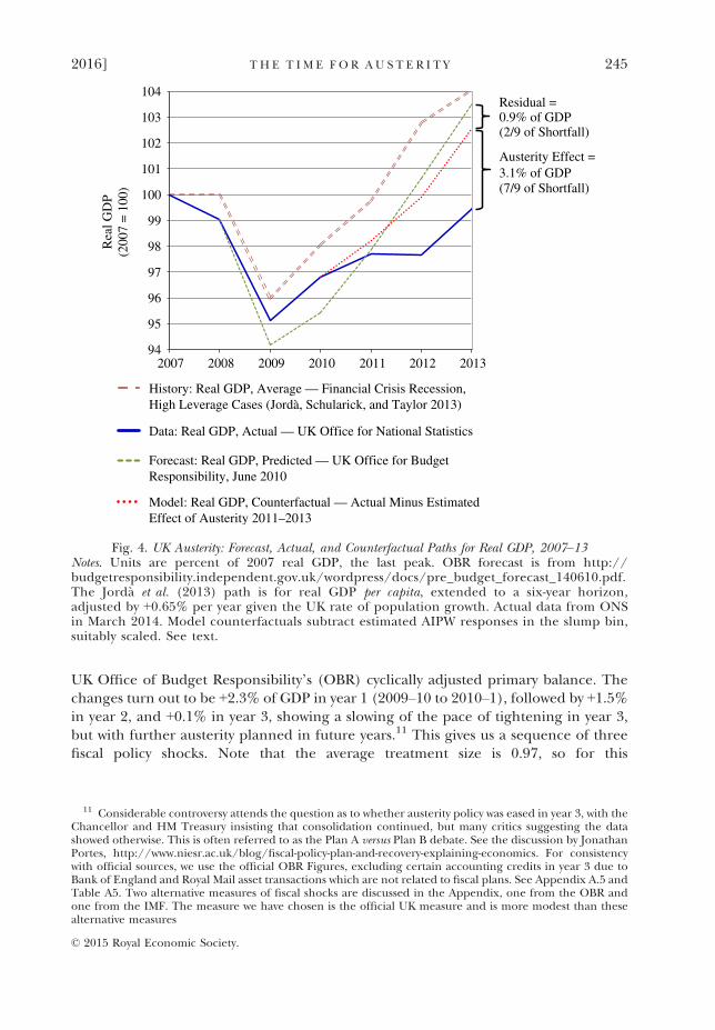
UK Office of Budget Responsibility’s (OBR) cyclically adjusted primary balance. Thechanges turn out to be +2.3% of GDP in year 1 (2009–10 to 2010–1), followed by +1.5%in year 2, and +0.1% in year 3, showing a slowing of the pace of tightening in year 3,but with further austerity planned in future years.11 This gives us a sequence of threefiscal policy shocks. Note that the average treatment size is 0.97, so for this

Austerity Effect =3.1% of GDP (7/9 of Shortfall)

Residual = 0.9% of GDP(2/9 of Shortfall)

94

Model: Real GDP, Counterfactual — Actual Minus EstimatedEffect of Austerity 2011–2013

95

96

97

98

99

100

101

102

103

104

Data: Real GDP, Actual — UK Office for National Statistics

History: Real GDP, Average — Financial Crisis Recession, High Leverage Cases (Jordà, Schularick, and Taylor 2013)

Forecast: Real GDP, Predicted — UK Office for BudgetResponsibility, June 2010

20082007 2009 2010 2011 2012 2013

Rea

l GD

P(2

007

= 1

00)

Fig. 4. UK Austerity: Forecast, Actual, and Counterfactual Paths for Real GDP, 2007–13Notes. Units are percent of 2007 real GDP, the last peak. OBR forecast is from http://budgetresponsibility.independent.gov.uk/wordpress/docs/pre_budget_forecast_140610.pdf.The Jord�a et al. (2013) path is for real GDP per capita, extended to a six-year horizon,adjusted by +0.65% per year given the UK rate of population growth. Actual data from ONSin March 2014. Model counterfactuals subtract estimated AIPW responses in the slump bin,suitably scaled. See text.

11 Considerable controversy attends the question as to whether austerity policy was eased in year 3, with theChancellor and HM Treasury insisting that consolidation continued, but many critics suggesting the datashowed otherwise. This is often referred to as the Plan A versus Plan B debate. See the discussion by JonathanPortes, http://www.niesr.ac.uk/blog/fiscal-policy-plan-and-recovery-explaining-economics. For consistencywith official sources, we use the official OBR Figures, excluding certain accounting credits in year 3 due toBank of England and Royal Mail asset transactions which are not related to fiscal plans. See Appendix A.5 andTable A5. Two alternative measures of fiscal shocks are discussed in the Appendix, one from the OBR andone from the IMF. The measure we have chosen is the official UK measure and is more modest than thesealternative measures



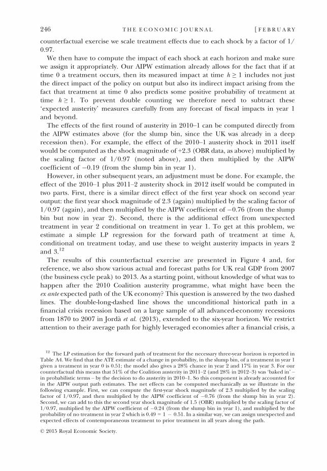
counterfactual exercise we scale treatment effects due to each shock by a factor of 1/0.97.

We then have to compute the impact of each shock at each horizon and make surewe assign it appropriately. Our AIPW estimation already allows for the fact that if attime 0 a treatment occurs, then its measured impact at time h ≥ 1 includes not justthe direct impact of the policy on output but also its indirect impact arising from thefact that treatment at time 0 also predicts some positive probability of treatment attime h ≥ 1. To prevent double counting we therefore need to subtract these‘expected austerity’ measures carefully from any forecast of fiscal impacts in year 1and beyond.

The effects of the first round of austerity in 2010–1 can be computed directly fromthe AIPW estimates above (for the slump bin, since the UK was already in a deeprecession then). For example, the effect of the 2010–1 austerity shock in 2011 itselfwould be computed as the shock magnitude of +2.3 (OBR data, as above) multiplied bythe scaling factor of 1/0.97 (noted above), and then multiplied by the AIPWcoefficient of �0.19 (from the slump bin in year 1).

However, in other subsequent years, an adjustment must be done. For example, theeffect of the 2010–1 plus 2011–2 austerity shock in 2012 itself would be computed intwo parts. First, there is a similar direct effect of the first year shock on second yearoutput: the first year shock magnitude of 2.3 (again) multiplied by the scaling factor of1/0.97 (again), and then multiplied by the AIPW coefficient of �0.76 (from the slumpbin but now in year 2). Second, there is the additional effect from unexpectedtreatment in year 2 conditional on treatment in year 1. To get at this problem, weestimate a simple LP regression for the forward path of treatment at time h,conditional on treatment today, and use these to weight austerity impacts in years 2and 3.12

The results of this counterfactual exercise are presented in Figure 4 and, forreference, we also show various actual and forecast paths for UK real GDP from 2007(the business cycle peak) to 2013. As a starting point, without knowledge of what was tohappen after the 2010 Coalition austerity programme, what might have been theex ante expected path of the UK economy? This question is answered by the two dashedlines. The double-long-dashed line shows the unconditional historical path in afinancial crisis recession based on a large sample of all advanced-economy recessionsfrom 1870 to 2007 in Jord�a et al. (2013), extended to the six-year horizon. We restrictattention to their average path for highly leveraged economies after a financial crisis, a

12 The LP estimation for the forward path of treatment for the necessary three-year horizon is reported inTable A4. We find that the ATE estimate of a change in probability, in the slump bin, of a treatment in year 1given a treatment in year 0 is 0.51; the model also gives a 28% chance in year 2 and 17% in year 3. For ourcounterfactual this means that 51% of the Coalition austerity in 2011–2 (and 28% in 2012–3) was ‘baked in’ –in probabilistic terms – by the decision to do austerity in 2010–1. So this component is already accounted forin the AIPW output path estimates. The net effects can be computed mechanically as we illustrate in thefollowing example. First, we can compute the first-year shock magnitude of 2.3 multiplied by the scalingfactor of 1/0.97, and then multiplied by the AIPW coefficient of �0.76 (from the slump bin in year 2).Second, we can add to this the second year shock magnitude of 1.5 (OBR) multiplied by the scaling factor of1/0.97, multiplied by the AIPW coefficient of �0.24 (from the slump bin in year 1), and multiplied by theprobability of no treatment in year 2 which is 0.49 = 1 � 0.51. In a similar way, we can assign unexpected andexpected effects of contemporaneous treatment to prior treatment in all years along the path.



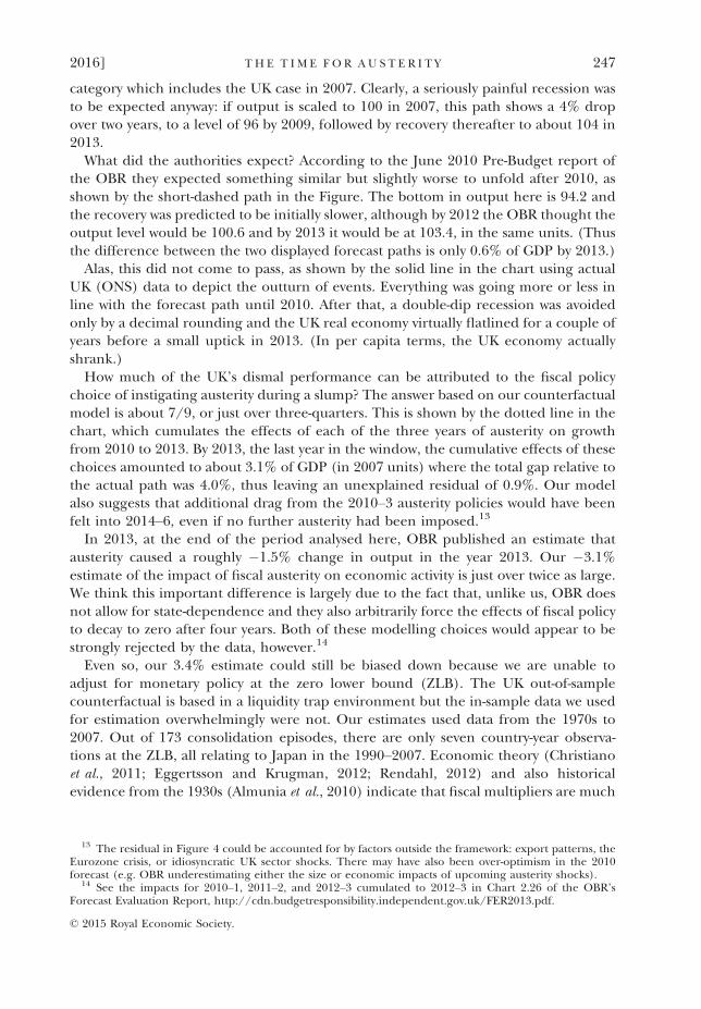
category which includes the UK case in 2007. Clearly, a seriously painful recession wasto be expected anyway: if output is scaled to 100 in 2007, this path shows a 4% dropover two years, to a level of 96 by 2009, followed by recovery thereafter to about 104 in2013.

What did the authorities expect? According to the June 2010 Pre-Budget report ofthe OBR they expected something similar but slightly worse to unfold after 2010, asshown by the short-dashed path in the Figure. The bottom in output here is 94.2 andthe recovery was predicted to be initially slower, although by 2012 the OBR thought theoutput level would be 100.6 and by 2013 it would be at 103.4, in the same units. (Thusthe difference between the two displayed forecast paths is only 0.6% of GDP by 2013.)

Alas, this did not come to pass, as shown by the solid line in the chart using actualUK (ONS) data to depict the outturn of events. Everything was going more or less inline with the forecast path until 2010. After that, a double-dip recession was avoidedonly by a decimal rounding and the UK real economy virtually flatlined for a couple ofyears before a small uptick in 2013. (In per capita terms, the UK economy actuallyshrank.)

How much of the UK’s dismal performance can be attributed to the fiscal policychoice of instigating austerity during a slump? The answer based on our counterfactualmodel is about 7/9, or just over three-quarters. This is shown by the dotted line in thechart, which cumulates the effects of each of the three years of austerity on growthfrom 2010 to 2013. By 2013, the last year in the window, the cumulative effects of thesechoices amounted to about 3.1% of GDP (in 2007 units) where the total gap relative tothe actual path was 4.0%, thus leaving an unexplained residual of 0.9%. Our modelalso suggests that additional drag from the 2010–3 austerity policies would have beenfelt into 2014–6, even if no further austerity had been imposed.13

In 2013, at the end of the period analysed here, OBR published an estimate thatausterity caused a roughly �1.5% change in output in the year 2013. Our �3.1%estimate of the impact of fiscal austerity on economic activity is just over twice as large.We think this important difference is largely due to the fact that, unlike us, OBR doesnot allow for state-dependence and they also arbitrarily force the effects of fiscal policyto decay to zero after four years. Both of these modelling choices would appear to bestrongly rejected by the data, however.14

Even so, our 3.4% estimate could still be biased down because we are unable toadjust for monetary policy at the zero lower bound (ZLB). The UK out-of-samplecounterfactual is based in a liquidity trap environment but the in-sample data we usedfor estimation overwhelmingly were not. Our estimates used data from the 1970s to2007. Out of 173 consolidation episodes, there are only seven country-year observa-tions at the ZLB, all relating to Japan in the 1990–2007. Economic theory (Christianoet al., 2011; Eggertsson and Krugman, 2012; Rendahl, 2012) and also historicalevidence from the 1930s (Almunia et al., 2010) indicate that fiscal multipliers are much

13 The residual in Figure 4 could be accounted for by factors outside the framework: export patterns, theEurozone crisis, or idiosyncratic UK sector shocks. There may have also been over-optimism in the 2010forecast (e.g. OBR underestimating either the size or economic impacts of upcoming austerity shocks).

14 See the impacts for 2010–1, 2011–2, and 2012–3 cumulated to 2012–3 in Chart 2.26 of the OBR’sForecast Evaluation Report, http://cdn.budgetresponsibility.independent.gov.uk/FER2013.pdf.



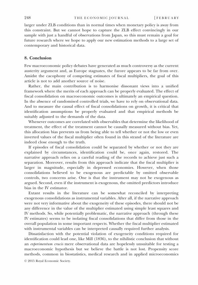
larger under ZLB conditions than in normal times when monetary policy is away fromthis constraint. But we cannot hope to capture the ZLB effect convincingly in oursample with just a handful of observations from Japan, so this must remain a goal forfuture research where we hope to apply our new estimation methods to a large set ofcontemporary and historical data.

8. Conclusion

Few macroeconomic policy debates have generated as much controversy as the currentausterity argument and, as Europe stagnates, the furore appears to be far from over.Amidst the cacophony of competing estimates of fiscal multipliers, the goal of thisarticle is not to add another source of noise.

Rather, the main contribution is to harmonise dissonant views into a unifiedframework where the merits of each approach can be properly evaluated. The effect offiscal consolidation on macroeconomic outcomes is ultimately an empirical question.In the absence of randomised controlled trials, we have to rely on observational data.And to measure the causal effect of fiscal consolidations on growth, it is critical thatidentification assumptions be properly evaluated and that empirical methods besuitably adjusted to the demands of the data.

Whenever outcomes are correlated with observables that determine the likelihood oftreatment, the effect of the treatment cannot be causally measured without bias. Yet,this allocation bias prevents us from being able to tell whether or not the low or eveninverted values of the fiscal multiplier often found in this strand of the literature areindeed close enough to the truth.

If episodes of fiscal consolidation could be separated by whether or not they areexplained by circumstances, identification could be, once again, restored. Thenarrative approach relies on a careful reading of the records to achieve just such aseparation. Moreover, results from this approach indicate that the fiscal multiplier islarger in magnitude, especially in depressed economies. However, when thoseconsolidations believed to be exogenous are predictable by omitted observablecontrols, two concerns arise. One is that the instrument may not be exogenous asargued. Second, even if the instrument is exogenous, the omitted predictors introducebias in the IV estimator.

Extant results in the literature can be somewhat reconciled by interpretingexogenous consolidations as instrumental variables. After all, if the narrative approachwere not very informative about the exogeneity of these episodes, there should not beany difference in the value of the multiplier estimated using simple least squares andIV methods. So, while potentially problematic, the narrative approach (through theseIV estimates) seems to be isolating fiscal consolidations that differ from those in theoverall population in some important respects. Whether the fiscal multiplier estimatedwith instrumental variables can be interpreted causally required further analysis.

Dissatisfaction with the potential violation of exogeneity conditions required foridentification could lead one, like Mill (1836), to the nihilistic conclusion that withoutan experimentum crucis mere observational data are hopelessly unsuitable for testing amacroeconomic hypothesis but we believe the battle is not lost. Propensity scoremethods, common in biostatistics, medical research and in applied microeconomics



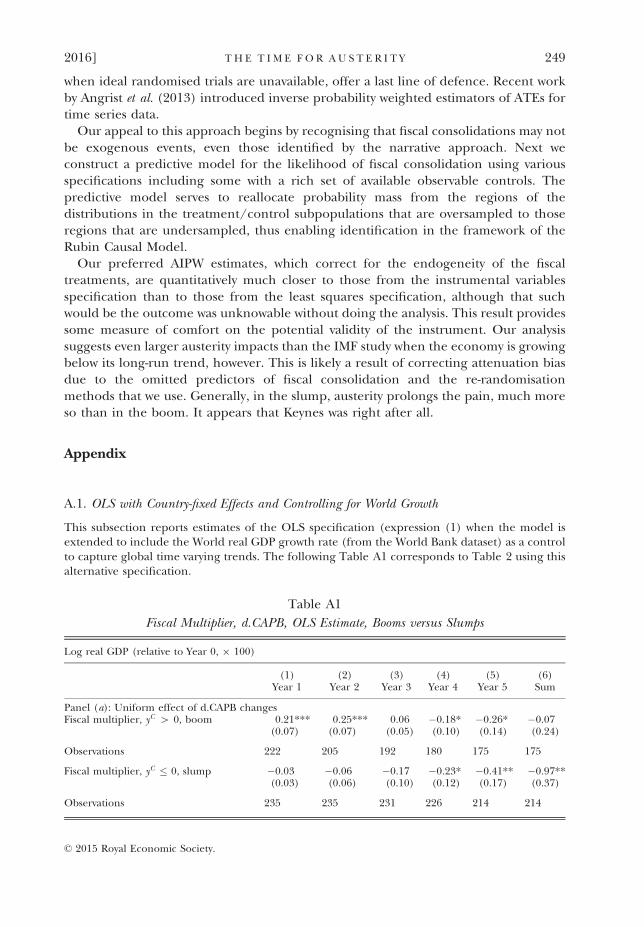
when ideal randomised trials are unavailable, offer a last line of defence. Recent workby Angrist et al. (2013) introduced inverse probability weighted estimators of ATEs fortime series data.

Our appeal to this approach begins by recognising that fiscal consolidations may notbe exogenous events, even those identified by the narrative approach. Next weconstruct a predictive model for the likelihood of fiscal consolidation using variousspecifications including some with a rich set of available observable controls. Thepredictive model serves to reallocate probability mass from the regions of thedistributions in the treatment/control subpopulations that are oversampled to thoseregions that are undersampled, thus enabling identification in the framework of theRubin Causal Model.

Our preferred AIPW estimates, which correct for the endogeneity of the fiscaltreatments, are quantitatively much closer to those from the instrumental variablesspecification than to those from the least squares specification, although that suchwould be the outcome was unknowable without doing the analysis. This result providessome measure of comfort on the potential validity of the instrument. Our analysissuggests even larger austerity impacts than the IMF study when the economy is growingbelow its long-run trend, however. This is likely a result of correcting attenuation biasdue to the omitted predictors of fiscal consolidation and the re-randomisationmethods that we use. Generally, in the slump, austerity prolongs the pain, much moreso than in the boom. It appears that Keynes was right after all.

Appendix

A.1. OLS with Country-fixed Effects and Controlling for World Growth

This subsection reports estimates of the OLS specification (expression (1) when the model isextended to include the World real GDP growth rate (from the World Bank dataset) as a controlto capture global time varying trends. The following Table A1 corresponds to Table 2 using thisalternative specification.

Table A1

Fiscal Multiplier, d.CAPB, OLS Estimate, Booms versus Slumps

Log real GDP (relative to Year 0, 9 100)


Panel (a): Uniform effect of d.CAPB changesFiscal multiplier, yC [ 0, boom 0.21*** 0.25*** 0.06 �0.18* �0.26* �0.07

(0.07) (0.07) (0.05) (0.10) (0.14) (0.24)

Observations 222 205 192 180 175 175

Fiscal multiplier, yC � 0, slump �0.03 �0.06 �0.17 �0.23* �0.41** �0.97**(0.03) (0.06) (0.10) (0.12) (0.17) (0.37)

Observations 235 235 231 226 214 214



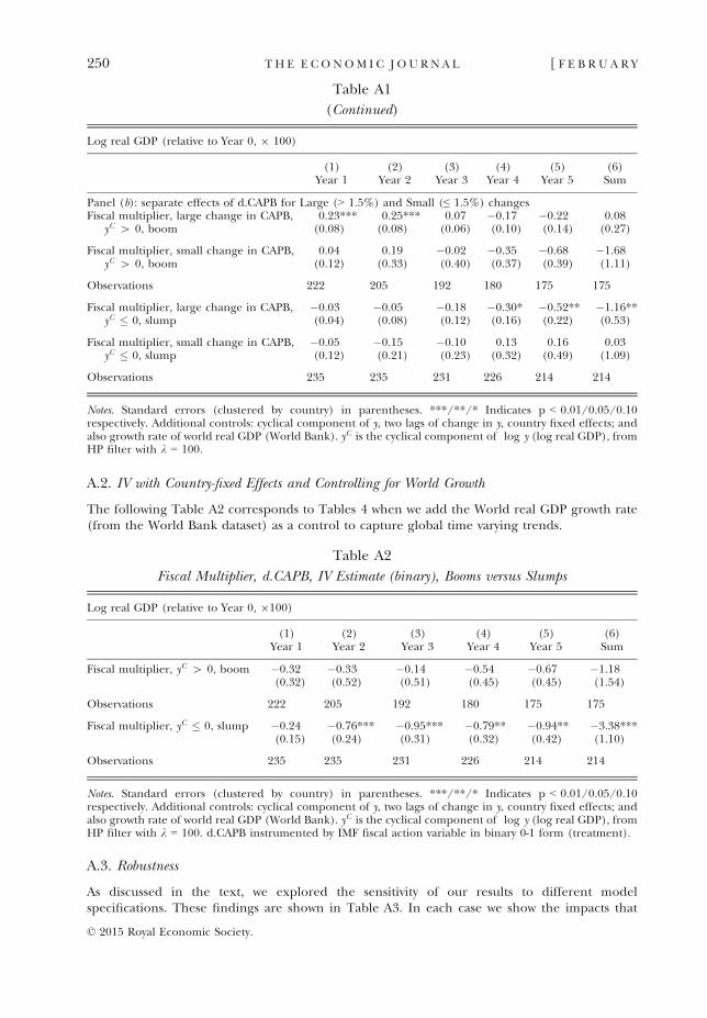
A.2. IV with Country-fixed Effects and Controlling for World Growth

The following Table A2 corresponds to Tables 4 when we add the World real GDP growth rate(from the World Bank dataset) as a control to capture global time varying trends.

A.3. Robustness

As discussed in the text, we explored the sensitivity of our results to different modelspecifications. These findings are shown in Table A3. In each case we show the impacts that

Table A1

(Continued)

Log real GDP (relative to Year 0, 9 100)


Panel (b): separate effects of d.CAPB for Large (> 1.5%) and Small (≤ 1.5%) changesFiscal multiplier, large change in CAPB,

yC [ 0, boom0.23*** 0.25*** 0.07 �0.17 �0.22 0.08(0.08) (0.08) (0.06) (0.10) (0.14) (0.27)

Fiscal multiplier, small change in CAPB,yC [ 0, boom

0.04 0.19 �0.02 �0.35 �0.68 �1.68(0.12) (0.33) (0.40) (0.37) (0.39) (1.11)

Observations 222 205 192 180 175 175

Fiscal multiplier, large change in CAPB,yC � 0, slump

�0.03 �0.05 �0.18 �0.30* �0.52** �1.16**(0.04) (0.08) (0.12) (0.16) (0.22) (0.53)

Fiscal multiplier, small change in CAPB,yC � 0, slump

�0.05 �0.15 �0.10 0.13 0.16 0.03(0.12) (0.21) (0.23) (0.32) (0.49) (1.09)

Observations 235 235 231 226 214 214

Notes. Standard errors (clustered by country) in parentheses. ***/**/* Indicates p < 0.01/0.05/0.10respectively. Additional controls: cyclical component of y, two lags of change in y, country fixed effects; andalso growth rate of world real GDP (World Bank). yC is the cyclical component of log y (log real GDP), fromHP filter with k = 100.

Table A2

Fiscal Multiplier, d.CAPB, IV Estimate (binary), Booms versus Slumps

Log real GDP (relative to Year 0, 9100)


Fiscal multiplier, yC [ 0, boom �0.32 �0.33 �0.14 �0.54 �0.67 �1.18(0.32) (0.52) (0.51) (0.45) (0.45) (1.54)

Observations 222 205 192 180 175 175

Fiscal multiplier, yC � 0, slump �0.24 �0.76*** �0.95*** �0.79** �0.94** �3.38***(0.15) (0.24) (0.31) (0.32) (0.42) (1.10)

Observations 235 235 231 226 214 214

Notes. Standard errors (clustered by country) in parentheses. ***/**/* Indicates p < 0.01/0.05/0.10respectively. Additional controls: cyclical component of y, two lags of change in y, country fixed effects; andalso growth rate of world real GDP (World Bank). yC is the cyclical component of log y (log real GDP), fromHP filter with k = 100. d.CAPB instrumented by IMF fiscal action variable in binary 0-1 form (treatment).



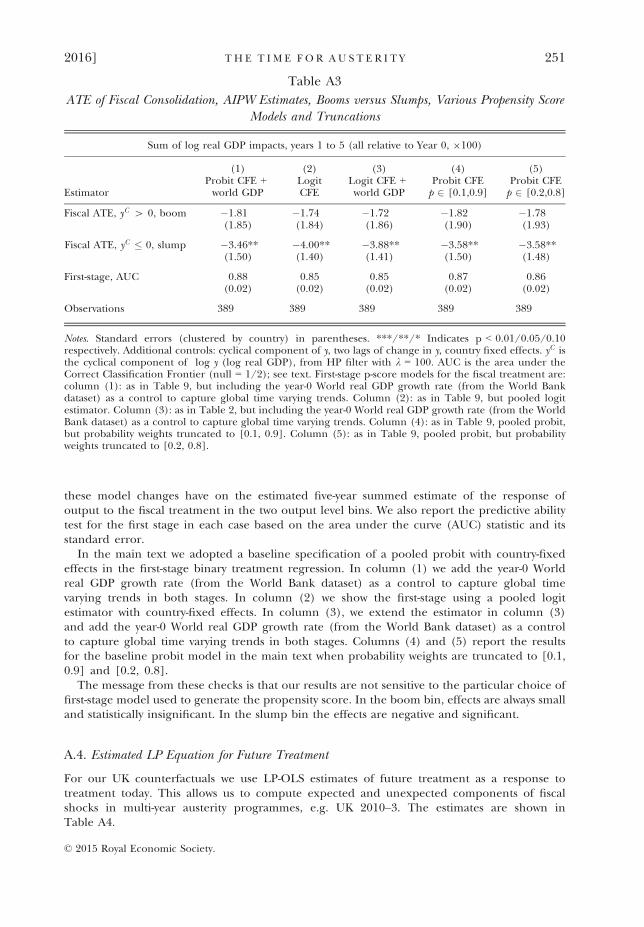
these model changes have on the estimated five-year summed estimate of the response ofoutput to the fiscal treatment in the two output level bins. We also report the predictive abilitytest for the first stage in each case based on the area under the curve (AUC) statistic and itsstandard error.

In the main text we adopted a baseline specification of a pooled probit with country-fixedeffects in the first-stage binary treatment regression. In column (1) we add the year-0 Worldreal GDP growth rate (from the World Bank dataset) as a control to capture global timevarying trends in both stages. In column (2) we show the first-stage using a pooled logitestimator with country-fixed effects. In column (3), we extend the estimator in column (3)and add the year-0 World real GDP growth rate (from the World Bank dataset) as a controlto capture global time varying trends in both stages. Columns (4) and (5) report the resultsfor the baseline probit model in the main text when probability weights are truncated to [0.1,0.9] and [0.2, 0.8].

The message from these checks is that our results are not sensitive to the particular choice offirst-stage model used to generate the propensity score. In the boom bin, effects are always smalland statistically insignificant. In the slump bin the effects are negative and significant.

A.4. Estimated LP Equation for Future Treatment

For our UK counterfactuals we use LP-OLS estimates of future treatment as a response totreatment today. This allows us to compute expected and unexpected components of fiscalshocks in multi-year austerity programmes, e.g. UK 2010–3. The estimates are shown inTable A4.

Table A3

ATE of Fiscal Consolidation, AIPW Estimates, Booms versus Slumps, Various Propensity ScoreModels and Truncations

Sum of log real GDP impacts, years 1 to 5 (all relative to Year 0, 9100)

Estimator

(1) (2) (3) (4) (5)Probit CFE +world GDP

LogitCFE

Logit CFE +world GDP

Probit CFEp 2 [0.1,0.9]

Probit CFEp 2 [0.2,0.8]

Fiscal ATE, yC [ 0, boom �1.81 �1.74 �1.72 �1.82 �1.78(1.85) (1.84) (1.86) (1.90) (1.93)

Fiscal ATE, yC � 0, slump �3.46** �4.00** �3.88** �3.58** �3.58**(1.50) (1.40) (1.41) (1.50) (1.48)

First-stage, AUC 0.88 0.85 0.85 0.87 0.86(0.02) (0.02) (0.02) (0.02) (0.02)

Observations 389 389 389 389 389

Notes. Standard errors (clustered by country) in parentheses. ***/**/* Indicates p < 0.01/0.05/0.10respectively. Additional controls: cyclical component of y, two lags of change in y, country fixed effects. yC isthe cyclical component of log y (log real GDP), from HP filter with k = 100. AUC is the area under theCorrect Classification Frontier (null = 1/2); see text. First-stage p-score models for the fiscal treatment are:column (1): as in Table 9, but including the year-0 World real GDP growth rate (from the World Bankdataset) as a control to capture global time varying trends. Column (2): as in Table 9, but pooled logitestimator. Column (3): as in Table 2, but including the year-0 World real GDP growth rate (from the WorldBank dataset) as a control to capture global time varying trends. Column (4): as in Table 9, pooled probit,but probability weights truncated to [0.1, 0.9]. Column (5): as in Table 9, pooled probit, but probabilityweights truncated to [0.2, 0.8].



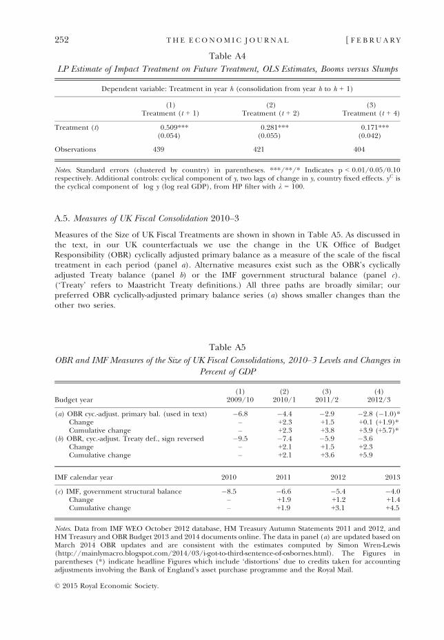
A.5. Measures of UK Fiscal Consolidation 2010–3

Measures of the Size of UK Fiscal Treatments are shown in shown in Table A5. As discussed inthe text, in our UK counterfactuals we use the change in the UK Office of BudgetResponsibility (OBR) cyclically adjusted primary balance as a measure of the scale of the fiscaltreatment in each period (panel a). Alternative measures exist such as the OBR’s cyclicallyadjusted Treaty balance (panel b) or the IMF government structural balance (panel c).(‘Treaty’ refers to Maastricht Treaty definitions.) All three paths are broadly similar; ourpreferred OBR cyclically-adjusted primary balance series (a) shows smaller changes than theother two series.

Table A4

LP Estimate of Impact Treatment on Future Treatment, OLS Estimates, Booms versus Slumps

Dependent variable: Treatment in year h (consolidation from year h to h + 1)

(1) (2) (3)Treatment (t + 1) Treatment (t + 2) Treatment (t + 4)

Treatment (t) 0.509*** 0.281*** 0.171***(0.054) (0.055) (0.042)

Observations 439 421 404

Notes. Standard errors (clustered by country) in parentheses. ***/**/* Indicates p < 0.01/0.05/0.10respectively. Additional controls: cyclical component of y, two lags of change in y, country fixed effects. yC isthe cyclical component of log y (log real GDP), from HP filter with k = 100.

Table A5

OBR and IMF Measures of the Size of UK Fiscal Consolidations, 2010–3 Levels and Changes inPercent of GDP

Budget year(1) (2) (3) (4)

2009/10 2010/1 2011/2 2012/3

(a) OBR cyc.-adjust. primary bal. (used in text) �6.8 �4.4 �2.9 �2.8 (�1.0)*Change – +2.3 +1.5 +0.1 (+1.9)*Cumulative change – +2.3 +3.8 +3.9 (+5.7)*

(b) OBR, cyc.-adjust. Treaty def., sign reversed �9.5 �7.4 �5.9 �3.6Change – +2.1 +1.5 +2.3Cumulative change – +2.1 +3.6 +5.9

IMF calendar year 2010 2011 2012 2013

(c) IMF, government structural balance �8.5 �6.6 �5.4 �4.0Change – +1.9 +1.2 +1.4Cumulative change – +1.9 +3.1 +4.5

Notes. Data from IMF WEO October 2012 database, HM Treasury Autumn Statements 2011 and 2012, andHM Treasury and OBR Budget 2013 and 2014 documents online. The data in panel (a) are updated based onMarch 2014 OBR updates and are consistent with the estimates computed by Simon Wren-Lewis(http://mainlymacro.blogspot.com/2014/03/i-got-to-third-sentence-of-osbornes.html). The Figures inparentheses (*) indicate headline Figures which include ‘distortions’ due to credits taken for accountingadjustments involving the Bank of England’s asset purchase programme and the Royal Mail.



Federal Reserve Bank of San Francisco and University of California, DavisUniversity of California, Davis, NBER, and CEPR

Submitted: 3 November 2014Accepted: 15 July 2015

Additional Supporting Information may be found in the online version of this article:

Data S1.

ReferencesAlesina, A. and Ardagna, S. (2010). ‘Large changes in fiscal policy: taxes versus spending’, in (J.R. Brown,

ed.), Tax Policy and the Economy, pp. 35–68, Chicago, IL: University of Chicago Press.Alesina, A. and Perotti, R. (1995). ‘Fiscal expansions and adjustments in OECD economies’, Economic Policy,

vol. 10(21), pp. 207–47.Almunia, M., B�en�etrix, A., Eichengreen, B., O’Rourke, K.H. and Rua, G. (2010). ‘From great depression to

great credit crisis: similarities, differences and lessons’, Economic Policy, vol. 25(62), pp. 219–65.Angrist, J.D., Jord�a, O. and Kuersteiner, G.M. (2013). ‘Semiparametric estimates of monetary policy effects:

string theory revisited’, NBER Working Paper No. 19355.Angrist, J.D., and Kuersteiner, G.M. (2004). ‘Semiparametric causality tests using the policy propensity score’,

NBER Working Paper No. 10975.Angrist, J.D., and Kuersteiner, G.M. (2011). ‘Causal effects of monetary shocks: semiparametric conditional

independence tests with a multinomial propensity score’, Review of Economics and Statistics, vol. 93(3),pp. 725–47.

Angrist, J.D., and Pischke, J. (2010). ‘The credibility revolution in empirical economics: how better researchdesign is taking the con out of econometrics’, Journal of Economic Perspectives, vol. 24(2), pp. 3–30.

Ardagna, S. (2004). ‘Fiscal stabilizations: when do they work and why’, European Economic Review, vol. 48(5),pp. 1047–74.

Auerbach, A.J. and Gorodnichenko, Y. (2012). ‘Measuring the output responses to fiscal policy’, AmericanEconomic Journal: Economic Policy, vol. 4(2), pp. 1–27.

Auerbach, A.J. and Gorodnichenko, Y. (2013). ‘Fiscal multipliers in recession and expansion’, in (A. Alesinaand F. Giavazzi, eds.), Fiscal Policy after the Financial Crisis, pp. 98–102, Chicago, IL: University of ChicagoPress.

Barro, R.J. and Redlick, C.J. (2011). ‘Macroeconomic effects from government purchases and taxes’, QuarterlyJournal of Economics, vol. 126(1), pp. 51–102.

Blanchard, O.J. (1993). ‘Suggestion for a new set of fiscal indicators’, OECD Economics DepartmentWorking Paper No. 79.

Born, B., M€uller, G. and Pfeifer, G. (2015). ‘Does austerity pay off?’ CEPR Discussion Paper No. 10425.Cameron, C.A. and Trivedi P.K. (2005). Microeconometrics: Methods and Applications, Cambridge: Cambridge

University Press.Chalmers, I. (2005). ‘Statistical theory was not the reason that randomisation was used in the British Medical

Research Council’s clinical trial of streptomycin for pulmonary tuberculosis’, in (G. Jorland, A. Opinel,and G. Weisz, eds.), Body Counts: Medical Quantification in Historical and Sociological Perspectives, pp. 309–34,Montreal: McGill-Queens University Press.

Chalmers, I. (2011). ‘Why the 1948 MRC trial of streptomycin used treatment allocation based on randomnumbers’, Journal of the Royal Society of Medicine, vol. 104(9), pp. 383–86.

Christiano, L., Eichenbaum, M. and Rebelo, S. (2011). ‘When is the government spending multiplier large?’,Journal of Political Economy, vol. 119(1), pp. 78–121.

Cole, S.R. and Hern�an, M.A. (2008). ‘Constructing inverse probability weights for marginal structuralmodels’, American Journal of Epidemiology, vol. 186(6), pp. 656–64.

Davies, G. (2012). ‘Why is the UK recovery weaker than the US?’, Financial Times, November 14. Available at:http://blogs.ft.com/gavyndavies/2012/11/14/why-is-the-uk-recovery-weaker-than-the-us/ (last accessed:4 November 2015).

Donaldson, I.M.L. (2016). ‘Petrarch’s letter to Boccaccio “on the proud and presumptuous behaviour ofphysicians”’, JLL Bulletin: Commentaries on the history of treatment evaluation. Available at: http://www.jameslindlibrary.org/articles/petrarchs-letter-to-boccaccio-on-the-proud-and-presumptuous-behaviour-of-physicians/.



Eggertsson, G.B., and Krugman, P. (2012). ‘Debt, deleveraging, and the liquidity trap: a Fisher-Minsky-Kooapproach’, Quarterly Journal of Economics, vol. 127(3), pp. 1469–513.

Giavazzi, F. and Pagano, M. (1990). ‘Can severe fiscal contractions be expansionary? Tales of two smalleuropean countries’, in (O.J. Blanchard and S. Fischer, eds.), NBER Macroeconomics Annual 1990, pp. 75–122, Cambridge, MA: MIT Press.

Glynn, A.N., and Quinn, K.M. (2010). ‘An introduction to the augmented inverse propensity weightedestimator’, Political Analysis, vol. 18(1), pp. 36–56.

Guajardo, J., Leigh, D. and Pescatori, A. (2014). ‘Expansionary austerity: new international evidence’, Journalof the European Economic Association, vol. 12(4), pp. 949–68.

Heckman, J.J. (1976). ‘The common structure of statistical models of truncation, sample selection, andlimited dependent variables and a simple estimator for such models’, Annals of Economic and SocialMeasurement, vol. 5(4), pp. 475–92.

Hern�andez de Cos, P. and Moral-Benito, E. (2013). ‘Fiscal consolidations and economic growth’, FiscalStudies, vol. 34(4), pp. 491–515.

Hirano, K., Imbens, G.W. and Ridder, G. (2003). ‘Efficient estimation of average treatment effects using theestimated propensity score’, Econometrica, vol. 71(4), pp. 1161–89.

Horvitz, D.G. and Thompson, D.J. (1952). ‘A generalization of sampling without replacement from a finitepopulation’, Journal of the American Statistical Association, vol. 47(260), pp. 663–85.

Imbens, G.W. (2004). ‘Nonparametric estimation of average treatment effects under exogeneity: a review’,Review of Economics and Statistics, vol. 86(1), pp. 4–29.

Jord�a, O. (2005). ‘Estimation and inference of impulse responses by local projections’, American EconomicReview, vol. 95(1), pp. 161–82.

Jord�a, O., Schularick, M. and Taylor A.M. (2013). ‘When credit bites back’, Journal of Money, Credit andBanking, vol. 45(s2), pp. 3–28.

Jord�a, O. and Taylor, A.M. (2011). ‘Performance evaluation of zero net-investment strategies’, NBERWorking Paper No. 17150.

Keynes, J.M. (1937). ‘How to avoid a slump’, The Times, 12–14th January.Kreif, N., Grieve, R., Radice, R.and Sekhon, J.S. (2013). ‘Regression-adjusted matching and double-robust

methods for estimating average treatment effects in health economic evaluation’, Health Services andOutcomes Research Methodology, vol. 13(2–4), pp. 174–202.

Leeper, E.M. (1997). ‘Narrative and VAR approaches to monetary policy: common identification problems’,Journal of Monetary Economics, vol. 40(3), pp. 641–57.

Lunceford, J.K. and Davidian, M. (2004). ‘Stratification and weighting via the propensity score in estimationof causal treatment effects: a comparative study’, Statistics in Medicine, vol. 23(19), pp. 2937–60.

Mertens, K. and Ravn, M.O. (2013). ‘The dynamic effects of personal and corporate income tax changes inthe United States’, American Economic Review, vol. 103(4), pp. 1212–47.

Mertens, K. and Ravn, M.O. (2014). ‘A reconciliation of SVAR and narrative estimates of tax multipliers’,Journal of Monetary Economics, vol. 68(S), pp. S1–19.

Mill, J. (1836). ‘On the definition of political economy; and on the method of philosophical investigation inthat science’, London and Westminster Review, vol. 26(1), pp. 1–29.

Mountford, A. and Uhlig, H. (2009). ‘What are the effects of fiscal policy shocks?’, Journal of AppliedEconometrics, vol. 24(6), pp. 960–92.

Nakamura, E. and Steinsson, J. (2014). ‘Fiscal stimulus in a monetary union: evidence from US regions’,American Economic Review, vol. 104(3), pp. 753–92.

Owyang, M.T., Ramey, V.A. and Zubairy, S. (2013). ‘Are government spending multipliers greater duringperiods of slack? Evidence from twentieth-century historical data’, American Economic Review, vol. 103(3),pp. 129–34.

Parker, J.A. (2011). ‘On measuring the effects of fiscal policy in recessions’, Journal of Economic Literature, vol.49(3), pp. 703–18.

Perotti, R. (1999). ‘Fiscal policy in good times and bad’,Quarterly Journal of Economics, vol. 114(4), pp. 1399–436.Perotti, R. (2013). ‘The austerity myth: gain without pain?’, in (A. Alesina and F. Giavazzi, eds.), Fiscal Policy

after the Financial Crisis, pp. 307–54, Chicago, IL: University of Chicago Press.Posen, A. (2012). Why is their recovery better than ours? (Even though neither is good enough.) Speech at

the National Institute of Economic and Social Research, London, 27 March. Available at: http://www.bankofengland.co.uk/publications/Documents/speeches/2012/speech560.pdf (last accessed: 4November 2015).

Ramey, V.A. and Shapiro, M.D. (1998). ‘Costly capital reallocation and the effects of government spending’,Carnegie-Rochester Conference Series on Public Policy, vol. 48(1), pp. 145–94.

Rendahl, P. (2012). ‘Fiscal policy in an unemployment crisis’, Cambridge Working Papers in Economics1211.

Robins, J.M. (2000). ‘Robust estimation in sequentially ignorable missing data and causal inference models’,Proceedings of the American Statistical Association Section on Bayesian Statistical Science 1999, pp. 6–10,Alexandria, VA: American Statistical Association.



Robins, J.M. and Rotnitzky, A. (1995). ‘Semiparametric efficiency in multivariate regression models’, Journalof the American Statistical Association, vol. 90(429), pp. 122–9.

Robins, J.M., Rotnitzky, A. and Zhao, L.P. (1994). ‘Estimation of regression coefficients when some regressorsare not always observed’, Journal of the American Statistical Association, vol. 89(427), pp. 846–66.

Robins, J.M., Rotnitzky, A. and Zhao, L.P. (1995). ‘Analysis of semiparametric regression models for repeatedoutcomes in the presence of missing data’, Journal of the American Statistical Association, vol. 90(429), pp.106–21.

Romer, C.D. and Romer, D.H. (1989). ‘Does monetary policy matter? A new test in the spirit of Friedman andSchwartz’, in (O.J. Blanchard and S. Fischer, eds.), NBER Macroeconomics Annual 1989, pp. 121–70,Cambridge, MA: MIT Press.

Romer, C.D. and Romer, D.H. (1997). ‘Identification and the narrative approach: a reply to Leeper’, Journalof Monetary Economics, vol. 40(3), pp. 659–65.

Rosenbaum, P.R. and Rubin, D.B. (1983). ‘The central role of the propensity score in observational studiesfor causal effects’, Biometrika, vol. 70(1), pp. 41–55.

Scharfstein, D.O., Rotnitzky, A. and Robins, J.M. (1999). ‘Adjusting for nonignorable drop-out usingsemiparametric nonresponse models: rejoinder’, Journal of the American Statistical Association, vol. 94(448),pp. 1135–46.

Schularick, M. and Taylor, A.M. (2012). ‘Fact-checking financial recessions: US-UK update’, VoxEU, October24. Available at: http://www.voxeu.org/article/fact-checking-financial-recessions-us-uk-update (lastaccessed: 4 November 2015).

Stock, J.H. and Watson, M.W. (2012). ‘Disentangling the channels of the 2007–09 recession’, Brookings Paperson Economic Activity, Spring, pp. 81–156.

Wooldridge, J.M. (1997). ‘Quasi-likelihood methods for count data’, in (M. H. Pesaran and P. Schmidt, eds.),Handbook of Applied Econometrics, vol. 2, pp. 352–406, Oxford: Blackwell.

Wooldridge, J.M. (2007). ‘Inverse probability weighted M-estimation for general missing data problems’,Journal of Econometrics, vol. 141(2), pp. 1281–301.

Wooldridge, J.M. (2010). Econometric Analysis of Cross Section and Panel Data, 2nd edn, Cambridge, MA: MITPress.



Copyright of Economic Journal is the property of Wiley-Blackwell and its content may not becopied or emailed to multiple sites or posted to a listserv without the copyright holder'sexpress written permission. However, users may print, download, or email articles forindividual use.