Embed Size (px)
Citation preview
The College of Wooster LibrariesOpen Works
Senior Independent Study Theses
2013
The Truth About Lie Symmetries: SolvingDifferential Equations With Symmetry MethodsRuth A. SteinhourThe College of Wooster, [email protected]
Follow this and additional works at: https://openworks.wooster.edu/independentstudy
Part of the Applied Mathematics Commons
This Senior Independent Study Thesis Exemplar is brought to you by Open Works, a service of The College of Wooster Libraries. It has been acceptedfor inclusion in Senior Independent Study Theses by an authorized administrator of Open Works. For more information, please [email protected].
© Copyright 2013 Ruth A. Steinhour
Recommended CitationSteinhour, Ruth A., "The Truth About Lie Symmetries: Solving Differential Equations With Symmetry Methods" (2013). SeniorIndependent Study Theses. Paper 949.https://openworks.wooster.edu/independentstudy/949
The Truth About Lie SymmetriesSolving Differential EquationsWith
SymmetryMethods
Independent Study Thesis
Presented in Partial Fulfillment of the Requirements forthe Degree Bachelor of Arts in the
Department of Mathematics and Computer Scienceat The College of Wooster
byRuth Steinhour
The College of Wooster2013
Advised by:
Dr. Jennifer Bowen and Dr. Robert Wooster


c© 2013 by Ruth Steinhour

iv
Abstract
Differential equations are vitally important in numerous scientific fields.
Oftentimes, they are quite challenging to solve. This Independent Study examines
one method for solving differential equations. Norwegian mathematician Sophus
Lie developed this method, which uses groups of symmetries, called Lie groups.
These symmetries map one solution curve to another. They can be used to
determine a canonical coordinate system for a given differential equation. Writing
the differential equation in terms of a different coordinate system can make the
equation simpler to solve. This I.S. explores techniques for finding a canonical
coordinate system and using it to solve a given differential equation. Several
examples are presented.
v

vi

Acknowledgments
First and foremost I would like to thank Professor Jennifer Bowen and Professor
Robert Wooster for their advice and support. I would also like to thank my parents,
Sarah and Wayne Steinhour, my sister, Elizabeth Steinhour, and my friends, both on
campus and off, for their continued encouragement.
vii

viii
Contents
Abstract v
Acknowledgments vii
Contents ix
CHAPTER PAGE
1 Introduction and Symmetries 11.1 Introduction . . . . . . . . . . . . . . . . . . . . . . . . . . . . . . . . . 11.2 Symmetries . . . . . . . . . . . . . . . . . . . . . . . . . . . . . . . . . 21.3 Lie Groups . . . . . . . . . . . . . . . . . . . . . . . . . . . . . . . . . . 51.4 The Symmetry Condition . . . . . . . . . . . . . . . . . . . . . . . . . 101.5 A Change in Coordinates . . . . . . . . . . . . . . . . . . . . . . . . . 151.6 Orbits . . . . . . . . . . . . . . . . . . . . . . . . . . . . . . . . . . . . . 20
2 Unearthing New Coordinates 232.1 The Tangent Vectors . . . . . . . . . . . . . . . . . . . . . . . . . . . . . 232.2 Canonical Coordinates . . . . . . . . . . . . . . . . . . . . . . . . . . . 272.3 A New Way to Solve Differential Equations . . . . . . . . . . . . . . . 342.4 The Linearized Symmetry Condition . . . . . . . . . . . . . . . . . . . 39
3 Infinitesimal Generators 513.1 Infinitesimal Generator . . . . . . . . . . . . . . . . . . . . . . . . . . . 513.2 Infinitesimal Generator in Canonical Coordinates . . . . . . . . . . . 57
4 Higher Order Differential Equations 614.1 The Symmetry Condition for Higher Order Differential Equations . . 614.2 The Linearized Symmetry Condition, Revisited . . . . . . . . . . . . . 64
5 Conclusion 73
References 75
ix

x
CHAPTER 1
Introduction and Symmetries
1.1 Introduction
Differential equations are used to model numerous phenomenon in our world, from
the spread of infectious diseases to the behavior of tidal waves. Naturally, the study
of differential equations plays a vital role in the physical sciences. These equations
are often non-linear and solving them requires unique and creative methods.
This Independent Study will explore the use of Lie symmetry groups for solving
differential equations. Sophus Lie (pronounced Lee), a Norwegian mathematician
born in 1842, developed these techniques [3]. He was the first to discover the
relationship between group theory and traditional methods for finding solution
curves [3]. His ground-breaking discovery involved using groups of point
transformations to solve differential equations [3].
This IS is the culmination of a two-semester exploration of Lie symmetry groups
and their role in solving differential equations. Chapters 1, 2, and 3 explore first
order differential equations. In Chapter 1, we define some basic terminology and
familiarize the reader with a few examples. Chapter 2 includes a variety of
1
2 1. Introduction and Symmetries
examples that illustrate how Lie Symmetries are utilized to solve both linear and
non-linear first order differential equations. The third chapter will define the
infinitesimal generator and discuss its role. The information presented in Chapter 3
can be extended for working with higher order differential equations. Chapter 4
discusses higher order differential equations and uses Lie Symmetry groups in a
preliminary example.
1.2 Symmetries
The information in this chapter is adapted from Hydon’s Symmetry Methods for
Differential Equations: A Beginner’s Guide [2] and Starrett’s “Solving Differential
Equations by Symmetry Groups" [5]. Material presented includes an introduction
to symmetry and Lie groups, along with preliminary examples. These examples
come from both sources.
The properties of symmetries provide a unique tool for solving differential
equations. A symmetry is a rigid mapping from an object to itself or another object.
It must preserve the structural properties of the original item. These mappings
include rotations, translations, and reflections. One simple example is S3, the group
of symmetries of a triangle. A group is a set that is closed under a binary operation.
Groups are associative under the operation, contain an identity element, and
inverses. The group S3 is a group of permutations that is closed under composition.
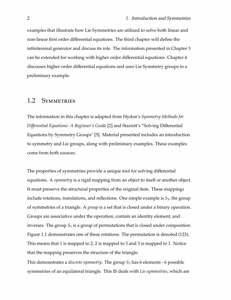
Figure 1.1 demonstrates one of these rotations. The permutation is denoted (123).
This means that 1 is mapped to 2, 2 is mapped to 3 and 3 is mapped to 1. Notice
that the mapping preserves the structure of the triangle.
This demonstrates a discrete symmetry. The group S3 has 6 elements - 6 possible
symmetries of an equilateral triangle. This IS deals with Lie symmetries, which are

1.2. Symmetries 3
Figure 1.1: Rotating symmetry of a triangle
not discrete.
Symmetries preserve structure. In other words, they must satisfy the symmetry
condition. In the previous example, satisfying the symmetry condition means that
the mapping is a bijection from an equilateral triangle to itself. Applied to the
solution curves of a differential equation, satisfying the symmetry condition
requires that a symmetry maps one solution curve to another. The resulting
solution curve must also satisfy the original differential equation. The symmetry
condition is crucial to solving differential equations with symmetry methods. We
will discuss this in greater detail in Section 1.4.
As a simple example of symmetry in differential equations, consider the following
ordinary differential equation (ODE),
dydx= 0. (1.1)
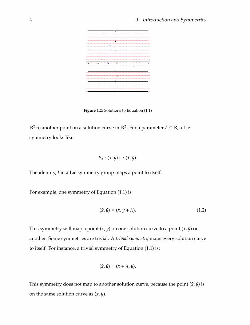
As one would expect the solutions to this equation are horizontal lines, seen in
Figure 1.2.
Lie symmetries are point transformations [6] that map a point on a solution curve in
4 1. Introduction and Symmetries
Figure 1.2: Solutions to Equation (1.1)
R2 to another point on a solution curve in R2. For a parameter λ ∈ R, a Lie
symmetry looks like:
Pλ : (x, y) #→ (x, y).
The identity, I in a Lie symmetry group maps a point to itself.
For example, one symmetry of Equation (1.1) is
(x, y) = (x, y + λ). (1.2)
This symmetry will map a point (x, y) on one solution curve to a point (x, y) on
another. Some symmetries are trivial. A trivial symmetry maps every solution curve
to itself. For instance, a trivial symmetry of Equation (1.1) is:
(x, y) = (x + λ, y).
This symmetry does not map to another solution curve, because the point (x, y) is
on the same solution curve as (x, y).
1.3. Lie Groups 5
1.3 Lie Groups
A Lie group is a group of symmetries with a parameter λ ∈ R. Lie group symmetries
are functions from R2 to R2. Let A be a set of points (x, y) ∈ R2 and let B be a set of
points (x, y) ∈ R2. A Lie group Pλ maps A to B:
Pλ : A #→ B.
Here, x is a function of x, y, and λ and y is also a function of x, y, and λ. Therefore,
a Lie group can also be written as
Pλ : (x, y) #→ ( f (x, y,λ), g(x, y,λ)).
Lie groups must meet the following restrictions:
1) Pλ is one-to-one and onto
2) Pλ2 ◦ Pλ1 = Pλ2+λ1
3) P0 = I
4) ∀λ1 ∈ R,∃λ2 = −λ1 such that Pλ2 ◦ Pλ1 = P0 = I
Equation (1.2) furnishes a simple example of a Lie group. The following is another
example of a Lie group that is a symmetry for Equation (1.1):
Pλ : (x, y) #→ (x, y) = (x, eλy). (1.3)
This is a symmetry because it maps a point on one solution curve of Equation (1.1)
to a point on another solution curve of Equation (1.1). We will show that it is a
symmetry for each fixed λ. It satisfies all of the properties of Lie symmetry groups:
1) The mapping (1.3) is one-to-one and onto.
This means that if two points (x1, y1) and (x2, y2) map to the same (x, y) then
(x1, y1) = (x2, y2) and for every (x, y) on the interval that (1.3) is defined (in this case,

6 1. Introduction and Symmetries
the entirety of R2), there is a point (x, y) that maps to (x, y). Consider the mapping
(1.3) for a fixed λ.We can clearly see that it is both one-to-one and onto for x
because x = x. This is the identity mapping. Now consider y = eλy. If we have
eλy1 = eλy2 = y, we can divide by eλ to see that y1 = y2. To show that there is a y
that corresponds with every y in R, we can divide y by eλ. Then y = e−λ y.
Therefore, the mapping (1.3) is one-to-one and onto.
2) The group satisfies the composition property of Lie groups.
Suppose we take Pλ2 ◦ Pλ1 . Apply Pλ1 to the point (x, y) to get
(x1, y1) = (x, eλ1 y).
Then apply Pλ2 to (x, eλ1 y) to get
(x2, y2) = (x, eλ2eλ1 y)
= (x, eλ2+λ1 y).
This is what we get when we apply Pλ2+λ1 , and therefore the composition property
is satisfied.
3) P0 is the identity:
(x, y) = (x, e0y) = (x, y).
4) For all λ1 ∈ R there is an inverse. When we apply P−λ1 ◦ Pλ1 , we get
(x, y) = (x, e−λ1(eλ1 y))
= (x, eλ1−λ1 y)
= (x, y).
1.3. Lie Groups 7
Therefore, all of the Lie group properties are satisfied, and the mapping (1.3) is a
symmetry group for Equation (1.1).
Lie groups might not necessarily be defined over the entire real number plane. We
will be dealing with local groups. The group action of a local group is not necessarily
defined over the entire real number plane [5]. Consider the next example.
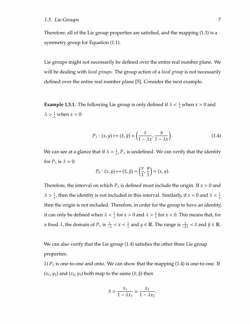
Example 1.3.1. The following Lie group is only defined if λ < 1x when x > 0 and
λ > 1x when x < 0:
Pλ : (x, y) #→ (x, y) =( x1 − λx
,y
1 − λx
). (1.4)
We can see at a glance that if λ = 1x , Pλ is undefined. We can verify that the identity
for Pλ is λ = 0:
P0 : (x, y) #→ (x, y) =(x1,
y1
)= (x, y).
Therefore, the interval on which Pλ is defined must include the origin. If x > 0 and
λ > 1x , then the identity is not included in this interval. Similarly, if x < 0 and λ < 1
x
then the origin is not included. Therefore, in order for the group to have an identity,
it can only be defined when λ < 1x for x > 0 and λ > 1
x for x < 0. This means that, for
a fixed λ, the domain of Pλ is 1−λ < x < 1
λ and y ∈ R. The range is 1−2λ < x and y ∈ R.
We can also verify that the Lie group (1.4) satisfies the other three Lie group
properties.
1) Pλ is one-to-one and onto. We can show that the mapping (1.4) is one-to-one. If
(x1, y2) and (x2, y2) both map to the same (x, y) then
x =x1
1 − λx1=
x2
1 − λx2.
8 1. Introduction and Symmetries
When we cross multiply we get
x1 − λx1x2 = x2 − λx1x2.
And therefore, x1 = x2. Similarly,
y =y1
1 − λx1=
y2
1 − λx2.
We have already shown that x1 = x2 therefore, y1 = y2. Thus (1.4) is one-to-one.
Now we can show that (1.4) is onto. Consider x:
x =x
1 − λx.
We can rewrite this equation as:
x = (1 − λx)x
x − λxx = x
x =x
1 − λx.
Now consider y:
y =y
1 − λx.
We can rewrite this as
y = (1 − λx)y = y − λxy
= y − λy( x1 − λx
)=
y1 − λx
.
Therefore, there is a point (x, y) that corresponds to every point (x, y) so the
1.3. Lie Groups 9
mapping is onto.
2) The group satisfies the composition property.
Suppose we take Pλ2 ◦ Pλ1 . The domain of this composition is 1−(λ1+λ2) < x < 1
(λ1+λ2)
and y ∈ R. The range is 1−2(λ1+λ2) < x and y ∈ R. Apply Pλ1 to (x, y) to get
(x1, y1) =( x1 − λ1x
,y
1 − λ1x
).
Then we can apply Pλ2 to (x1, y1) to find (x2, y2). For simplicity, we will compute x2
first:
x2 =x1
1 − λ2(x1)=
x1−λ1x
1 − λ2
(x
1−λ1x
)
=x
1 − λ1x· 1
1−λ1x−λ2x1−λ1x
=x
1 − λ1x· 1 − λ1x
1 − λ1x − λ2x
=x
1 − (λ1 + λ2)x.
Then we will compute y2:
y2 =y1
1 − λ2(x1)=
y1−λ1x
1 − λ2
(x
1−λ1x
)
=y
1 − λ1x· 1
1−λ1x−λ2x1−λ1x
=y
1 − λ1x· 1 − λ1x
1 − λ1x − λ2x
=y
1 − (λ1 + λ2)x.
Therefore, Pλ2 ◦ Pλ1 yields
(x2, y2) =(
x1 − (λ1 + λ2)x
,y
1 − (λ1 + λ2)x
).

10 1. Introduction and Symmetries
Similarly, if we apply Pλ1+λ2 to (x, y), we get
(x, y) =(
x1 − (λ1 + λ2)x
,y
1 − (λ1 + λ2)x
).
Therefore, the second Lie group property is satisfied.
3) We have already verified that P0 = I, the identity.
4) For all λ1 ∈ R, there exists an inverse. When we apply P−λ1 ◦ Pλ1 , we get
(x, y) =(
x1 − (λ1 − λ1)x
,y
1 − (λ1 − λ1)x
)= (x, y).
Therefore, the mapping (1.4) is a Lie group, defined only when λ < 1x when x > 0
and λ > 1x when x < 0.
1.4 The Symmetry Condition
The total derivative operator is important for understanding the symmetry condition.
The total derivative operator is:
Dx =∂∂x+
dydx∂∂y+
d2ydx2
∂∂y′.
First, consider an example that demonstrates how the total derivative operator
works.
Example 1.4.1. We will use the derivative operator to show that the family of
ellipsesx2
a2 +y2
b2 = c2 (1.5)
satisfies the differential equation
y′′ =y′(y − y′x)
yx. (1.6)
1.4. The Symmetry Condition 11
First, apply the total derivative operator to Equation (1.5):
2xa2 + y′
(2yb2
)= 0.
Then divide by 2, and rewrite the equation:
(1x
) (x2
a2
)+ y′( yb2
)= 0.
From Equation (1.5), we know that x2
a2 = c2 − y2
b2 . When we substitute this in, we get
(1x
) (c2 − y2
b2
)+ y′( yb2
)= 0.
Next, multiply by x
c2 − y2
b2 + y′( yx
b2
)= 0.
Next, apply the total derivative operator again:
y′yb2 + y′
(−2yb2 +
y′xb2
)+ y′′
( yxb2
)= 0.
Then multiply by b2:
y′y + y′(−2y + y′x) + y′′(yx) = 0.
From here, we can simplify to get
y′′ =y′(y − y′x)
yx.
In general, we are working with differential equations of the form:
dydx= ω(x, y). (1.7)
12 1. Introduction and Symmetries
In order to satisfy the symmetry condition, the point (x, y) must also be on a
solution curve to the differential equation (1.7):
dydx= ω(x, y). (1.8)
Written with the derivative operator, this looks like:
dydx=
DxyDxx
=yx +
dydx yy
xx +dydx xy
= ω(x, y).
From Equation (1.7), we know that dydx = ω(x, y). Therefore:
yx + ω(x, y)yy
xx + ω(x, y)xy= ω(x, y). (1.9)
Example 1.4.2. We will show that the differential equation
dydx=
1 − y2
x(1.10)
has a symmetry
(x, y) = (eλx, y). (1.11)
Substituting this into the symmetry condition, we want to get:
yx +dydx yy
xx +dydx xy
=1 − y2
x
oryx +
1−y2
x yy
xx +1−y2
x xy
=1 − y2
x. (1.12)
1.4. The Symmetry Condition 13
On the right side of Equation (1.12), we get:
1 − y2
x=
1 − y2
eλx.
On the left side, because yx = 0 and xy = 0, we get:
yx +1−y2
x yy
xx +1−y2
x xy
=
1−y2
x
eλ
=1 − y2
eλx.
Therefore, the symmetry condition is satisfied and (1.11) is a symmetry of (1.10).
Example 1.4.3. In the following example, we will demonstrate that the symmetry
(x, y) = (x, y + λe∫
F(x)dx) (1.13)
satisfies the differential equation
dydx= F(x)y + G(x).
We can test that the symmetry (1.13) meets the symmetry condition. First, we must
calculate yx, yy, xx, and yx:
yx = F(x)λe∫
F(x)dx
yy = 1
xx = 1
and
xy = 0.
Beginning with the left side of equation (1.9) and using the partial derivatives

14 1. Introduction and Symmetries
calculated above, we obtain
dydx= F(x)λe
∫F(x)dx + F(x)y + G(x)
= F(x)(y + λe
∫F(x)dx)+ G(x).
On the right side, we get
ω(x, y) = F(x)y + G(x)
= F(x)(y + λe
∫F(x)dx)+ G(x).
Example 1.4.4. In some cases, it is possible to use Equation (1.9) to determine the
symmetries of a differential equation. For example, consider
dydx= y. (1.14)
We want to find a symmetry of this equation that satisfies Equation (1.9). In other
words, the symmetry should satisfy the following:
yx + yyy
xx + yxy= y.
In order to find the symmetry, one can solve this equation for x and y. To make this
easier, one can make assumptions about x and y. Let’s assume that x is a function of
x and y and y maps to y
(x, y) = (x(x, y), y).
Then Equation (1.9) looks like:
yxx + yxy
= y.

1.5. A Change in Coordinates 15
Multiply by xx + yxy on both sides to get
y = y(xx + yxy).
As long as y ! 0, then
1 = xx + yxy.
We want to find a symmetry that will satisfy Equation (1.9). The following
symmetry does so:
(x, y) = (x + λ, y),λ ∈ R
because xx = 1 and xy = 0.
1.5 A Change in Coordinates
Oftentimes, a differential equation that is difficult to solve in Cartesian coordinates
becomes simpler in a different coordinate system. Any ODE that has a symmetry of
the form:
(x, y) = (x, y + λ) (1.15)
can be reduced to quadrature. This means that the differential equation can be
solved by an integrating technique. For all λ in some neighborhood of zero, the
symmetry condition reduces to:
ω(x, y) = ω(x, y + λ). (1.16)
We will differentiate Equation (1.16) with respect to λ at λ = 0. On the left side of
16 1. Introduction and Symmetries
the equation, we get ∂∂λω(x, y) = 0. On the right side, we can use the chain rule to
differentiate ω(x, y + λ) with respect to λ and therefore,
0 =∂ω∂x∂x∂λ+∂ω∂y∂y∂λ.
From Equation (1.16),∂x∂λ= 0
and∂y∂λ= 1.
Therefore, we have:
0 =∂ω∂y.
Thus the original ODE is a function of x only and then
dydx= ω(x)
and
y =∫ω(x)dx + c.
While a symmetry of the form in Equation (1.16) does not exist in Cartesian
coordinates for all differential equations (that would be nice!), it is possible to find
such a symmetry in a different coordinate system.
Example 1.5.1. The following differential equation becomes much simpler to
integrate when written in polar coordinates
dydx=
y3 + x2y − x − yx3 + xy2 − x + y
. (1.17)

1.5. A Change in Coordinates 17
If we let
x = r cosθ, y = r sinθ (1.18)
then
dx =∂x∂r
dr +∂x∂θ
dθ = cosθdr − r sinθdθ
and
dy =∂y∂r
dr +∂y∂θ
dθ = sinθdr + r cosθdθ.
We will simplify the right side of Equation (1.17) first, then substitute dydx on the left.
Substituting with Equations (1.18) to the right side, we get:
dydx=
r3 sin3 θ + r3 cos2 θ sinθ − r sinθ − r cosθr3 cos3 θ + r3 cosθ sin2 θ − r cosθ + r sinθ
.
This simplifies to:
dydx=
r3 sinθ(sin2 θ + cos2 θ) − r(cosθ + sinθ)r3 cosθ(cos2 θ + sin2 θ) + r(sinθ − cosθ)
=r2 sinθ − cosθ − sinθr2 cosθ + sinθ − cosθ
=sinθ(r2 − 1) − cosθcosθ(r2 − 1) + sinθ
. (1.19)
Now substitute dydx from Equation (1.19) above. The goal is to write the equation in
terms of drdθ :
dydx=
sinθdr + r cosθdθcosθdr − r sinθdθ
=sinθ(r2 − 1) − cosθcosθ(r2 − 1) + sinθ
.
Now one can cross multiply and solve the equation for drdθ :
(cosθ(r2 − 1)+ sinθ)(sinθdr+ r cosθdθ) = (sinθ(r2 − 1)− cosθ)(cosθdr− r sinθdθ).
18 1. Introduction and Symmetries
When we multiply through, we get
sinθ cosθ(r2 − 1)dr + r cos2 θ(r2 − 1)dθ + sin2 θdr + r cosθ sinθdθ
= sinθ cosθ(r2 − 1)dr − r sin2 θ(r2 − 1)dθ − cos2 θdr + r sinθ cosθ.
The sinθ cosθ(r2 − 1)dr term cancels, as well as the r cosθ sinθdθ term, to get:
r cos2 θ(r2 − 1)dθ + sin2 θdr = −r sin2 θ(r2 − 1)dθ − cos2 θdr.
This simplifies further:
dr = −r cos2 θ(r2 − 1)dθ − r sin2 θ(r2 − 1)dθ
which impliesdrdθ= −(r2 − 1)r(cos2 θ + sin2 θ)
and therefore:drdθ= r(1 − r2). (1.20)
This equation is separable in this coordinate system:
drr(1 − r2)
= dθ.
This requires the method of partial fractions to integrate:
∫1r
dr − 12
∫1
1 + rdr +
12
∫1
1 − rdr = θ.
When we integrate we get:
ln r − 12
ln(1 + r) − 12
ln(1 − r) = θ.
1.5. A Change in Coordinates 19
and
lnr√
1 − r2= θ.
Equation (1.20) has the symmetry
(r, θ) = (r,θ + λ)
which can be verified with the symmetry condition:
drdθ=
rθ + drdθ rr
θθ + drdθθr
= r(1 − r2).
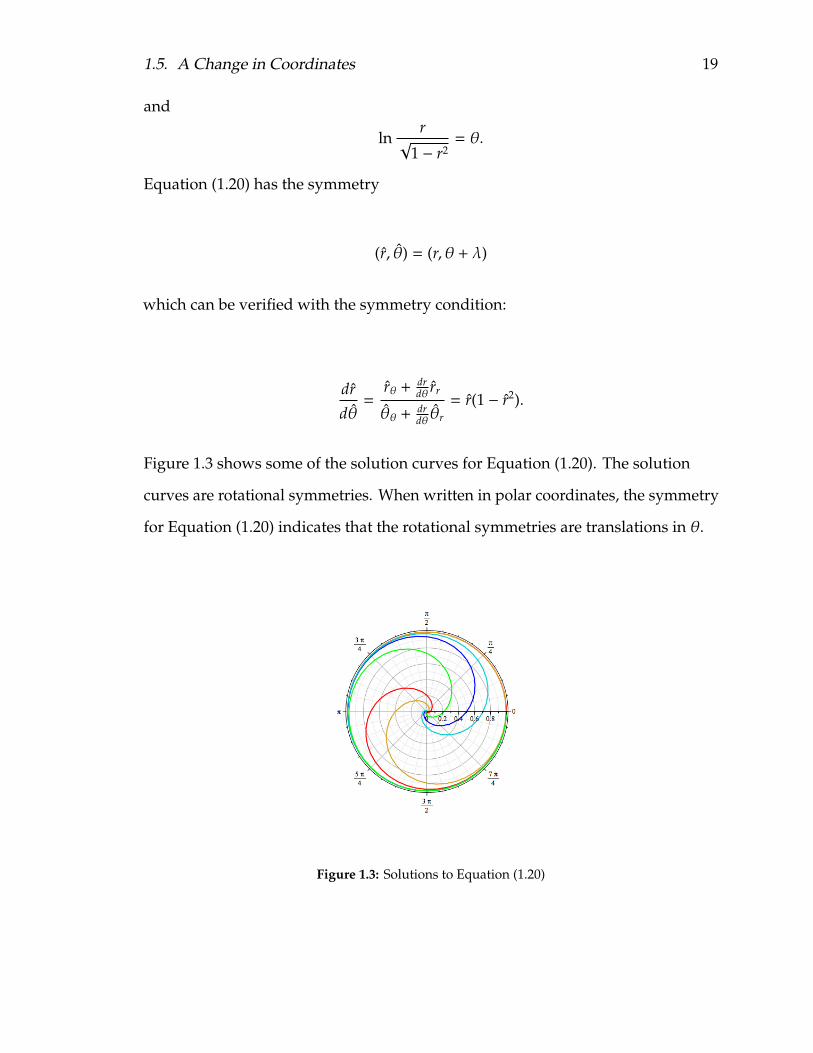
Figure 1.3 shows some of the solution curves for Equation (1.20). The solution
curves are rotational symmetries. When written in polar coordinates, the symmetry
for Equation (1.20) indicates that the rotational symmetries are translations in θ.
Figure 1.3: Solutions to Equation (1.20)

20 1. Introduction and Symmetries
1.6 Orbits
Orbits are an essential tool for solving differential equations using symmetry
methods. Suppose there is a point A on a solution curve to a differential equation.
Under a given symmetry, the orbit of A is the set of all points that A can be mapped
to for all possible values of λ.
Example 1.6.1. Consider the differential equation discussed in Section 1.2:
dydx= 0.
The orbits for the points on the solution curves of this differential equation are
vertical lines under the symmetry
(x, y) = (x, y + λ).
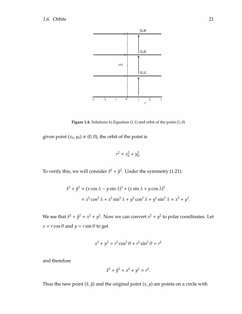
For instance, under the symmetry, the orbit of the point (1, 0) includes
{(1, 1), (1, 2), (1, 3), ...}.
Figure 1.4 shows the orbit of the point (1, 0) under the symmetry (x, y) = (x, y + λ).
Example 1.6.2. We have already seen a symmetry of Equation (1.17) when the
equation is expressed in polar coordinates. In Cartesian coordinates, one symmetry
of Equation (1.17) is
(x, y) = (x cosλ − y sinλ, x sinλ + y cosλ). (1.21)
The orbits of the points on the solution curves of Equation (1.17) are circles. For a
1.6. Orbits 21
Figure 1.4: Solutions to Equation (1.1) and orbit of the point (1, 0)
given point (x0, y0) ! (0, 0), the orbit of the point is
r2 = x20 + y2
0.
To verify this, we will consider x2 + y2. Under the symmetry (1.21):
x2 + y2 = (x cosλ − y sinλ)2 + (x sinλ + y cosλ)2
= x2 cos2 λ + x2 sin2 λ + y2 cos2 λ + y2 sin2 λ = x2 + y2.
We see that x2 + y2 = x2 + y2. Now we can convert x2 + y2 to polar coordinates. Let
x = r cosθ and y = r sinθ to get
x2 + y2 = r2 cos2 θ + r2 sin2 θ = r2
and therefore
x2 + y2 = x2 + y2 = r2.
Thus the new point (x, y) and the original point (x, y) are points on a circle with
22 1. Introduction and Symmetries
radius r. We can also see that the orbits of the points on the solution curves of
Equation (1.17) are circles by looking at a symmetry of Equation (1.17) in polar
coordinates. We saw in Section 1.5 that one symmetry is
(r, θ) = (r,θ + λ).
The radius remains constant as the symmetry takes one solution curve to another.
In Chapter 1 we have seen several examples of Lie symmetry groups and discussed
the significance of using a canonical coordinate system to solve first order
differential equations. An ODE that has a symmetry of the form
(x, y) = (x, y + λ)
can be reduced to quadrature. However, a symmetry of this form does not
necessarily exist in Cartesian coordinates for a given differential equation, hence
the importance of a canonical coordinate system. The next chapter will explain how
to find a new coordinate system and how to use it to solve first order ODE’s.
CHAPTER 2
UnearthingNew Coordinates
The material presented in this chapter is adapted from Chapter Two of Symmetry
Methods for Differential Equations: A Beginner’s Guide [2] and “Solving Differential
Equations by Symmetry Groups" [5]. The definitions and examples presented are
adapted from these sources. This chapter will explain how to find canonical
coordinates and how to use them to solve an ordinary differential equation.
As λ ∈ R varies under a given symmetry Pλ : (x, y) #→ (x, y), a point A travels along
its orbit. The tangent vectors to an orbit under a given symmetry are crucial to
determining the new coordinate system (r(x, y), s(x, y)). This chapter explains how
to find these tangent vectors, their importance, and how to use them to solve a
differential equation by symmetry methods.
2.1 The Tangent Vectors
The tangents to the orbit at any point (x, y) are described by the tangent vector in
the x direction, denoted ξ(x, y) and the tangent vector in the y direction, denoted
η(x, y). Thus
dxdλ= ξ(x, y)
23
24 2. Unearthing New Coordinates
anddydλ= η(x, y).
At the initial point (x, y), λ is equal to 0. Therefore
( dxdλ
∣∣∣∣∣λ=0,
dydλ
∣∣∣∣∣λ=0
)= (ξ(x, y), η(x, y)).
As we will demonstrate in Section 2.2, the tangent vectors ξ(x, y) and η(x, y) can be
used to find a simplifying coordinate system. However, ξ(x, y) and η(x, y) can
sometimes be used to find solution curves without the use of different coordinates.
The tangent vectors are useful for finding invariant solution curves. An invariant
solution curve is always mapped to itself under a symmetry. The points on an
invariant solution curve are mapped either to themselves or to another point on the
same curve [2]. Therefore, the orbit of a noninvariant point on an invariant solution
curve is the solution curve itself. If a solution curve is invariant that means that the
derivative at the point (x, y) will point in the same direction as the tangent vectors
to the orbit [2]. As λ varies, the point is mapped to another point on the same
solution curve, rather than a different solution curve. Therefore
dydx= ω(x, y) =
η(x, y)ξ(x, y)
.
The characteristic, Q is defined by Hydon [2] as
Q(x, y, y′) = η(x, y) − y′ξ(x, y). (2.1)
Because dydx = ω(x, y), we can rewrite Equation (2.1) as the reduced characteristic Q:
Q(x, y) = η(x, y) − ω(x, y)ξ(x, y). (2.2)

2.1. The Tangent Vectors 25
If, under a given symmetry, the reduced characteristic equals 0, then the solution
curve is invariant under that symmetry.
Example 2.1.1. The symmetry
(x, y) = (eλx, e(eλ−1)xy) (2.3)
acts trivially ondydx= y. (2.4)
In other words, every solution curve is invariant under the symmetry (2.3). To
show this, we will use the reduced characteristic, Equation (2.2). First we must find
ξ(x, y) and η(x, y). To get ξ(x, y), take the derivative of x with respect to λ:
ξ(x, y) = eλx.
To find ξ(x, y), evaluate ξ(x, y) at λ = 0 :
ξ(x, y) = x.
To obtain η(x, y) take the derivative of y with respect to λ:
η(x, y) = eλxe(eλ−1)xy.
To find η(x, y), evaluate η(x, y) at λ = 0 :
η(x, y) = xy.
Substituting these into the reduced characteristic, Q, we get
26 2. Unearthing New Coordinates
xy − xy = 0.
Therefore, the symmetry (2.3) acts trivially on Equation (2.4) because the reduced
characteristic equals 0.
Example 2.1.2. Consider the Riccati equation:
dydx= xy2 − 2y
x− 1
x3 , x ! 0. (2.5)
It has the following symmetry:
(x, y) = (eλx, e−2λy). (2.6)
The tangent vectors are
ξ(x, y) = x
and
η(x, y) = −2y.
The reduced characteristic is
Q(x, y) = −2y −(xy2 − 2y
x− 1
x3
)x
= −x2y2 +1x2 . (2.7)
Equation (2.7) is equal to 0 when y = ±x−2. Therefore, the symmetry (2.6) acts
nontrivially on all the solution curves of (2.5) except for y = x−2 and y = −x−2. This
example will be revisited in Section 2.3.
2.2. Canonical Coordinates 27
2.2 Canonical Coordinates
The goal of changing to a different coordinate system is to make a differential
equation easier to solve. As demonstrated in Section 1.3, if a differential equation
has a symmetry of the form
(x, y) = (x, y + λ),
then it can be reduced to quadrature and can be solved by an integrating technique.
However, not all differential equations have a symmetry of this form in Cartesian
coordinates. Therefore, one can change to a new coordinate system in
(r(x, y), s(x, y)) to obtain a symmetry:
Pλ : (r, s) #→ (r, s) = (r, s + λ).
The tangent vectors at (r, s) when λ = 0 are
drdλ
∣∣∣∣∣λ=0= 0 (2.8)
anddsdλ
∣∣∣∣∣λ=0= 1. (2.9)
Applying the chain rule to Equation (2.8) and Equation (2.9), we get
drdλ
∣∣∣∣∣λ=0=
drdx
dxdλ
∣∣∣∣∣λ=0+
drdy
dydλ
∣∣∣∣∣λ=0=
drdxξ(x, y) +
drdyη(x, y) = 0 (2.10)
anddsdλ
∣∣∣∣∣λ=0=
dsdx
dxdλ
∣∣∣∣∣λ=0+
dsdy
dydλ
∣∣∣∣∣λ=0=
dsdxξ(x, y) +
dsdyη(x, y) = 1. (2.11)
28 2. Unearthing New Coordinates
Equations (2.10) and (2.11) can also be written as [5]
rxξ(x, y) + ryη(x, y) = 0 (2.12)
and
sxξ(x, y) + syη(x, y) = 1. (2.13)
Equations (2.12) and (2.13) can be solved using the method of characteristics [5]. The
solutions to Equations (2.12) and (2.13), can be represented as surfaces, r(x, y) and
s(x, y), respectively. First consider Equation (2.12). This equation satisfies:
〈rx, ry,−1〉 ·〈 ξ, η, 0〉 = 0.
We know that the gradient of r(x, y) = z is 〈rx, ry,−1〉 and therefore, 〈rx, ry,−1〉 is a
normal vector to the surface r(x, y). Since the dot product 〈rx, ry,−1〉 ·〈 ξ, η, 0〉 = 0,
the vector 〈ξ(x, y), η(x, y), 0〉 is orthogonal to the normal vector. Thus
〈ξ(x, y), η(x, y), 0〉 is in the tangent plane to r(x, y).
Consider a parameterized curve, C on the surface r(x, y). Because 〈ξ(x, y), η(x, y), 0〉is in the tangent plane to the surface r(x, y), 〈ξ(x(t), y(t)), η(x(t), y(t)), 0〉 is tangent to
C. Therefore, we can write the symmetric equations as
dxdt= ξ,
dydt= η,
dzdt= 0.
These can also be written:dxξ=
dyη.
We can go through a similar process to find the symmetric equations for Equation
2.2. Canonical Coordinates 29
(2.13):dxdt= ξ,
dydt= η,
dzdt= 1
and thereforedxξ=
dyη= dz.
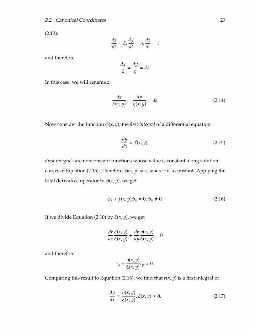
In this case, we will rename z:
dxξ(x, y)
=dyη(x, y)
= ds. (2.14)
Now consider the function φ(x, y), the first integral of a differential equation:
dydx= f (x, y). (2.15)
First integrals are nonconstant functions whose value is constant along solution
curves of Equation (2.15). Therefore, φ(x, y) = c, where c is a constant. Applying the
total derivative operator to φ(x, y), we get
φx + f (x, y)φy = 0,φy ! 0. (2.16)
If we divide Equation (2.10) by ξ(x, y), we get
drdxξ(x, y)ξ(x, y)
+drdyη(x, y)ξ(x, y)
= 0
and therefore
rx +η(x, y)ξ(x, y)
ry = 0.
Comparing this result to Equation (2.16), we find that r(x, y) is a first integral of
dydx=η(x, y)ξ(x, y)
, ξ(x, y) ! 0. (2.17)
30 2. Unearthing New Coordinates
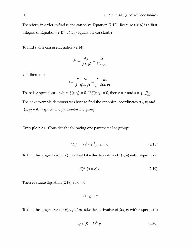
Therefore, in order to find r, one can solve Equation (2.17). Because r(x, y) is a first
integral of Equation (2.17), r(x, y) equals the constant, c.
To find s, one can use Equation (2.14):
ds =dyη(x, y)
=dxξ(x, y)
and therefore
s =∫
dyη(x, y)
=
∫dxξ(x, y)
.
There is a special case when ξ(x, y) = 0. If ξ(x, y) = 0, then r = x and s =∫ dyη(x,y) .
The next example demonstrates how to find the canonical coordinates r(x, y) and
s(x, y) with a given one parameter Lie group.
Example 2.2.1. Consider the following one parameter Lie group:
(x, y) = (eλx, ekλy), k > 0. (2.18)
To find the tangent vector ξ(x, y), first take the derivative of x(x, y) with respect to λ:
ξ(x, y) = eλx. (2.19)
Then evaluate Equation (2.19) at λ = 0:
ξ(x, y) = x.
To find the tangent vector η(x, y), first take the derivative of y(x, y) with respect to λ:
η(x, y) = kekλy. (2.20)

2.2. Canonical Coordinates 31
Then evaluate Equation (2.20) at λ = 0:
η(x, y) = ky.
Next, we use ξ(x, y) and η(x, y) to find r(x, y). Remember that r(x, y) is the first
integral ofdydx=η(x, y)ξ(x, y)
=kyx.
This equation is separable: ∫dyy= k∫
dxx.
Integrating this we get
ln y = ln xk + c0
which simplifies to
y = cxk.
When we solve for c, we get r(x, y) = yxk .
To find s, use Equation (2.14) to get
s =∫
dxξ(x, y)
=
∫dxx.
Therefore s = ln x. So the canonical coordinates are
(r, s) =( yxk , ln x
).
Example 2.2.2. Consider the following one parameter Lie group:
(x, y) =(
x(1 − λx)
,y
(1 − λx)
). (2.21)

32 2. Unearthing New Coordinates
We can start by finding the tangent vectors:
ξ(x, y) =x2
(1 − λx)2 (2.22)
and
η(x, y) =xy
(1 − λx)2 . (2.23)
Evaluating Equation (2.22) and (2.23) at λ = 0 results in:
(ξ(x, y), η(x, y)) = (x2, xy).
Therefore, we can integrate Equation (2.17) to find r(x, y):
dydx=η(x, y)ξ(x, y)
=yx.
This equation is separable: ∫dyy=
∫dxx.
When we integrate, we get:
ln y = ln x + c0.
Exponentiating and solving for r yields:
y = cx, c = r =yx.
To find s:
s =∫
dxx2 =
−1x.
Therefore, the canonical coordinates are
(r, s) =( y
x,−1x
).

2.2. Canonical Coordinates 33
The reader can see that the tangent vectors, rather than the symmetries themselves,
are used to find the canonical coordinates. This section and Section 2.1 explain how
to find the tangent vectors and use them when one knows the symmetry for a
differential equation. In practice the symmetry is often unknown. Section 2.4 will
explain how to find ξ(x, y) and η(x, y) without knowing the symmetry itself. Once
the tangent vectors and canonical coordinate system are determined, symmetries
can be reconstructed from the canonical coordinates. First, solve the canonical
coordinates r(x, y) and s(x, y) for x and y to get
x = f (r, s), y = g(r, s).
Then, x and y are
x = f (r, s) = f (r(x, y), s(x, y) + λ) (2.24)
and
y = g(r, s) = g(r(x, y), s(x, y) + λ). (2.25)
Example 2.2.3. We can find the symmetry associated with the following canonical
coordinates:
(r, s) =(y
x,−1x
).
Solving r and s for x and y, we get
x =−1s, y =
−rs.
34 2. Unearthing New Coordinates
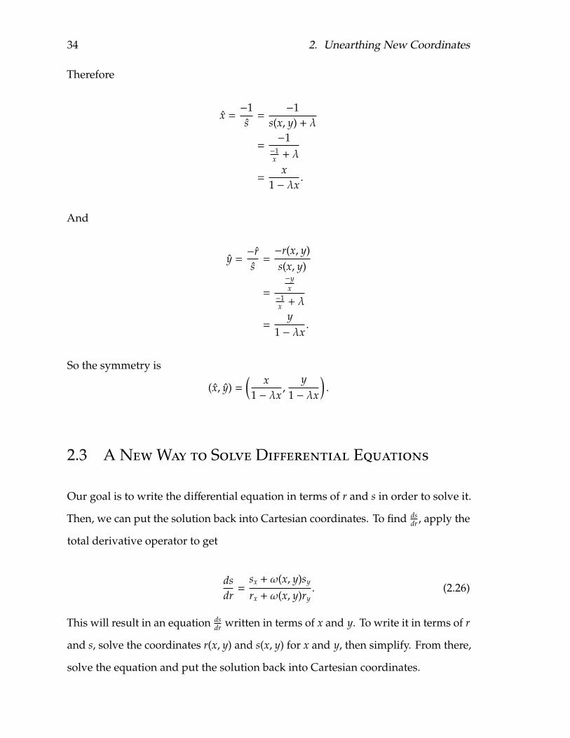
Therefore
x =−1s=
−1s(x, y) + λ
=−1
−1x + λ
=x
1 − λx.
And
y =−rs=−r(x, y)s(x, y)
=
−yx
−1x + λ
=y
1 − λx.
So the symmetry is
(x, y) =( x1 − λx
,y
1 − λx
).
2.3 A NewWay to Solve Differential Equations
Our goal is to write the differential equation in terms of r and s in order to solve it.
Then, we can put the solution back into Cartesian coordinates. To find dsdr , apply the
total derivative operator to get
dsdr=
sx + ω(x, y)sy
rx + ω(x, y)ry. (2.26)
This will result in an equation dsdr written in terms of x and y. To write it in terms of r
and s, solve the coordinates r(x, y) and s(x, y) for x and y, then simplify. From there,
solve the equation and put the solution back into Cartesian coordinates.

2.3. A New Way to Solve Differential Equations 35
Example 2.3.1. Again, consider the Riccati Equation:
dydx= xy2 − 2y
x− 1
x3 , x ! 0. (2.27)
It has the following symmetry:
(x, y) = (eλx, e−2λy).
This can be verified with the symmetry condition, Equation (1.9). First we will
calculate:
yx = 0, yy = e−2λ
and
xx = eλ, xy = 0.
Evaluating the left side of Equation (1.9) we get:
dydx=
e−2λ(xy2 − 2yx − 1
x3 )eλ
=1
e3λ
(xy2 − 2y
x− 1
x3
)
Evaluating the right side of Equation (1.9), we get:
dydx= eλx(e−2λy)2 − 2e−2λy
eλx− 1
(eλx)3 = e−3λxy2 − e−3λ(
2yx
)− e−3λ
( 1x3
)
=1
e3λ
(xy2 − 2y
x− 1
x3
).
Thus the symmetry condition is satisfied for the symmetry (x, y) = (eλx, e−2λy) of the
Riccati Equation. The tangent vectors for this symmetry are
ξ(x, y) = eλx, ξ(x, y) = x
36 2. Unearthing New Coordinates
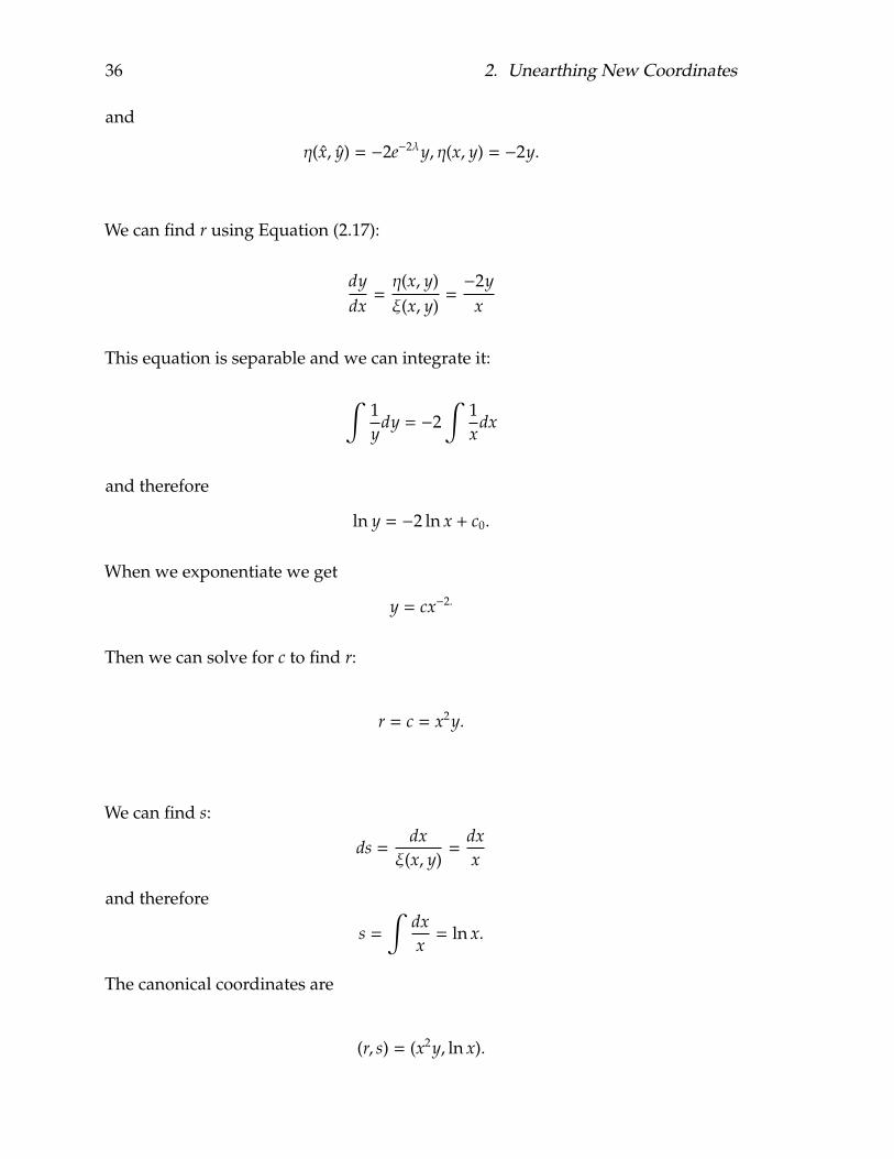
and
η(x, y) = −2e−2λy, η(x, y) = −2y.
We can find r using Equation (2.17):
dydx=η(x, y)ξ(x, y)
=−2y
x
This equation is separable and we can integrate it:
∫1y
dy = −2∫
1x
dx
and therefore
ln y = −2 ln x + c0.
When we exponentiate we get
y = cx−2.
Then we can solve for c to find r:
r = c = x2y.
We can find s:
ds =dxξ(x, y)
=dxx
and therefore
s =∫
dxx= ln x.
The canonical coordinates are
(r, s) = (x2y, ln x).
2.3. A New Way to Solve Differential Equations 37
We can write x and y in terms of r and s:
x = es
and
y = re−2s.
When we substitute the canonical coordinates into Equation (2.26), we get
dsdr=
1x
2xy + dydx x2
=1x
2xy + x3y2 − 2xy − 1x
=1
x4y2 − 1.
Then substitute in x = es and y = re−2s:
dsdr=
1e4sr2e−4s − 1
=1
r2 − 1.
Then we can integrate. The equation
dsdr=
1r2 − 1
is separable:
ds =dr
r2 − 1
and therefore
s =∫
drr2 − 1
.
38 2. Unearthing New Coordinates
We can integrate this using partial fractions:
s =12
∫1
r − 1dr − 1
2
∫1
r + 1dr
=12
(ln(r − 1) − ln(r + 1)) + k0
=12
ln(r − 1r + 1
)+ k0.
Then substitute r = x2y and s = ln x:
ln x =12
ln(x2y − 1x2y + 1
)+ k0.
We can exponentiate to get
x = k
√x2y − 1x2y + 1
.
Then we square both sides:
x2 = kx2y − 1x2y + 1
.
Simplification yields:
x2(x2y + 1) = k(x2y − 1)
x4y + x2 = kx2y − k
x4y − kx2y = −k − x2.
The solution to Equation (2.27) is
y =−k − x2
x4 − kx2 .
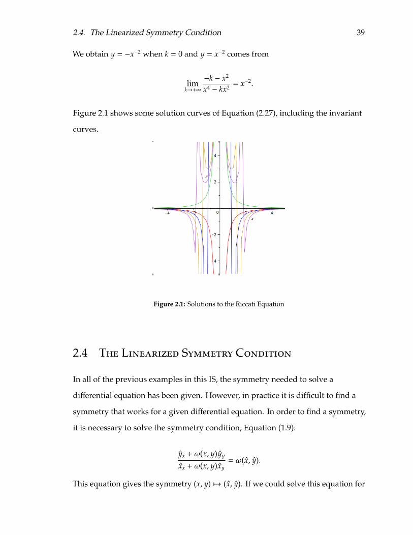
Recall from Section 2.1 that there are two invariant solution curves to the Riccati
equation under the symmetry (x, y) = (eλx, e−2λy). They are y = x−2 and y = −x−2.
2.4. The Linearized Symmetry Condition 39
We obtain y = −x−2 when k = 0 and y = x−2 comes from
limk→+∞
−k − x2
x4 − kx2 = x−2.
Figure 2.1 shows some solution curves of Equation (2.27), including the invariant
curves.
Figure 2.1: Solutions to the Riccati Equation
2.4 The Linearized Symmetry Condition
In all of the previous examples in this IS, the symmetry needed to solve a
differential equation has been given. However, in practice it is difficult to find a
symmetry that works for a given differential equation. In order to find a symmetry,
it is necessary to solve the symmetry condition, Equation (1.9):
yx + ω(x, y)yy
xx + ω(x, y)xy= ω(x, y).
This equation gives the symmetry (x, y) #→ (x, y). If we could solve this equation for
40 2. Unearthing New Coordinates
x and y then we could find the tangent vectors ξ and η and use them to find new
coordinates. However, this equation is often very difficult or impossible to solve.
Therefore, it is necessary to use a linearized symmetry condition to find ξ(x, y) and
η(x, y).
We can linearize the symmetry condition using a Taylor series expansion. We can
expand x, y and ω(x, y) around λ = 0.
x = x + λξ(x, y) +O(λ2) (2.28)
y = y + λη(x, y) +O(λ2) (2.29)
ω(x, y) = ω(x, y) + λ(ωx(x, y)ξ(x, y) + ωy(x, y)η(x, y)) +O(λ2) (2.30)
Here, O(λ2) describes the error function for the Taylor series expansions of x, y, and
ω(x, y). Consider an error function for one of the Taylor series expansions above.
We will denote it e(λ). As λ gets closer to 0, the ratio e(λ)λ2 approaches a constant, c. A
function e(λ) is O(λ2) if:
limλ→0
e(λ)λ2 = c.
We ignore terms of (λ)2 or higher. For simplicity, ξ(x, y) will be denoted merely as ξ
and η(x, y) as η.
To obtain the linearized symmetry condition, substitute Equations (2.28), (2.29),
(2.30) into the symmetry condition, Equation (1.9). For simplicity purposes, we will
compute the numerator, dy, first, then the denominator, dx, before simplifying the
entire equation. From Equation (2.29), we compute
yx = ληx
2.4. The Linearized Symmetry Condition 41
and
yy = 1 + ληy.
Therefore,
dy = ληx + ω(x, y) + ω(x, y)ληy
= ω + λ(ηx + ωηy)
And from Equation (2.28), we compute
xx = 1 + λξx
and
xy = λξy.
Therefore,
dx = 1 + λξx + ω(x, y)λξy
= 1 + λ(ξx + ωξy).
Now, we obtain that
dydx=ω + λ(ηx + ωηy)1 + λ(ξx + ωξy)
= ω(x, y).
Substitute Equation (2.30) for ω(x, y):
ω + λ(ηx + ωηy)1 + λ(ξx + ωξy)
= ω + λ(ωxξ + ωyη).
42 2. Unearthing New Coordinates
Then we multiply by the denominator to get:
ω + λ(ηx + ωηy) = (1 + λ(ξx + ωξy))(ω + λ(ωxξ + ωyη)).
Disregarding terms of λ2 or higher yields:
ω + λ(ηx + ωηy) = ω + λ(ωxξ + ωyη) + ωλ(ξx + ωξy).
Simplify further:
ηx + ωηy = ωxξ + ωyη + ωξx + ω2ξy.
This is the linearized symmetry condition:
ηx + (ηy − ξx)ω − ξyω2 = ξωx + ηωy. (2.31)
The next three examples demonstrate how to use the linearized symmetry
condition.
Example 2.4.1. Consider the equation,
dydx=
yx+ x. (2.32)
Substitute Equation (2.32) into the linearized symmetry condition, Equation (2.31)
to get
ηx + (ηy − ξx)ω − ξyω2 − (ξωx + ηωy) = 0
ηx − ξy
( yx+ x)2+(ηy − ξx
) ( yx+ x)−(ξ(1 − y
x2
)+ η(1x
))= 0.
It is necessary to solve this equation for ξ and η. In its current form, this is a very

2.4. The Linearized Symmetry Condition 43
difficult task. Therefore, we can make an ansatz (ansatz!) about ξ and η. Suppose
that ξ = 0 and η is a function of x only. Then we get
ηx −ηx= 0.
This differential equation is easily solved:
∫dηη=
∫dxx
ln η = ln x + c0
η = cx.
Now we can find the canonical coordinates r and s. Recall from Section 2.2 that
when ξ(x, y) = 0, r = x. To find s we can solve
ds =dyη.
Therefore
s =∫
dycx=
ycx.
Now set c = 1 to get
(r(x, y), s(x, y)) =(x,
yx
)
and
sx =−yx2 , sy =
1x.
Now we can substitute r and s into Equation (2.26) to obtain
dsdr=
−yx2 +
1x ( y
x + x)1
= 1.
44 2. Unearthing New Coordinates
Therefore, s = r + k, where k is a constant. Substituting x and y back in, we get
yx= x + k.
and the general solution to Equation (2.32) is
y = x2 + kx.
Example 2.4.2. Consider the differential equation:
dydx= e−xy2 + y + ex. (2.33)
We will use the linearized symmetry condition, Equation (2.31), to find the tangent
vectors ξ(x, y) and η(x, y). First, keep in mind that
ωx = −e−xy2 + ex
and
ωy = 2e−xy + 1.
We will make an ansatz about the form of ξ(x, y) and η(x, y). Suppose ξ = 1 and η is
a function of y only. Therefore, Equation (2.31) looks like
ηyω − ξωx − ηωy = 0
ηy(e−xy2 + y + ex) − (−e−xy2 + ex) − η(2e−xy + 1) = 0. (2.34)
Simplifying Equation (2.34) yields
e−xy(ηyy + y − 2η) + ex(ηy − 1) + ηyy − η = 0.
2.4. The Linearized Symmetry Condition 45
Therefore, we know that
ηyy + y − 2η = 0, (2.35)
ηyy − η = 0, (2.36)
and
ηy − 1 = 0. (2.37)
Solving Equation (2.37),dydη= 1
we get η = y. This is consistent with the Equations (2.35) and (2.36). Now we can
find the canonical coordinates. To find r, solve
dydx=ηξ= y.
This is separable. Integrating, we get ln y = x + c0 which simplifies to
y = cex
and therefore,
r =yex .
To find s:
s =∫
dx = x.
Therefore, the canonical coordinates are
(r, s) =( yex , x).
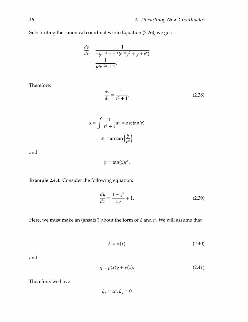
46 2. Unearthing New Coordinates
Substituting the canonical coordinates into Equation (2.26), we get:
dsdr=
1−ye−x + e−x(e−xy2 + y + ex)
=1
y2e−2x + 1.
Therefore:dsdr=
1r2 + 1
. (2.38)
s =∫
1r2 + 1
dr = arctan(r)
x = arctan( yex
)
and
y = tan(x)ex.
Example 2.4.3. Consider the following equation:
dydx=
1 − y2
xy+ 1. (2.39)
Here, we must make an (ansatz!) about the form of ξ and η. We will assume that
ξ = α(x) (2.40)
and
η = β(x)y + γ(x). (2.41)
Therefore, we have
ξx = α′, ξy = 0

2.4. The Linearized Symmetry Condition 47
and
ηx = β′y + γ′, ηy = β.
We can substitute these assumptions into the linearized symmetry condition (2.31).
First compute ωx and ωy :
ωx =y2 − 1
x2y
and
ωy =(−2y)(xy) − x(1 − y2)
(xy)2 =−2xy2 − x + xy2
(x2y2)
=−x(1 + y2)
x2y2 =−(1 + y2)
xy2 .
Then substitute Equation (2.40) and Equation (2.41) into Equation (2.31).
β′y + γ′ + (β − α′)(
1 − y2
xy+ 1)= α
(y2 − 1
x2y
)− (βy + γ)
(1 + y2
xy2
)(2.42)
Expanding and simplifying Equation (2.42) yields the following:
β′y + γ′ +β − α′
xy− (β − α′)y2
xy+ β − α′ = αy2
x2y− α
x2y− (βy + γ)
xy2 − (βy + γ)y2
xy2
β′y + γ′ +β − α′
xy+
(α′ − β)yx
+ β − α′ = αyx2 −
αx2y− βy
xy2 −γ
xy2 −βy3
xy2 −γy2
xy2
β′y + γ′ +β − α′
xy+
(α′ − β)yx
+ β − α′ = αyx2 −
αx2y− β
xy− βy
x− γ
xy2 −γx.
In comparing the powers of y, we get
y−2 : γ = 0
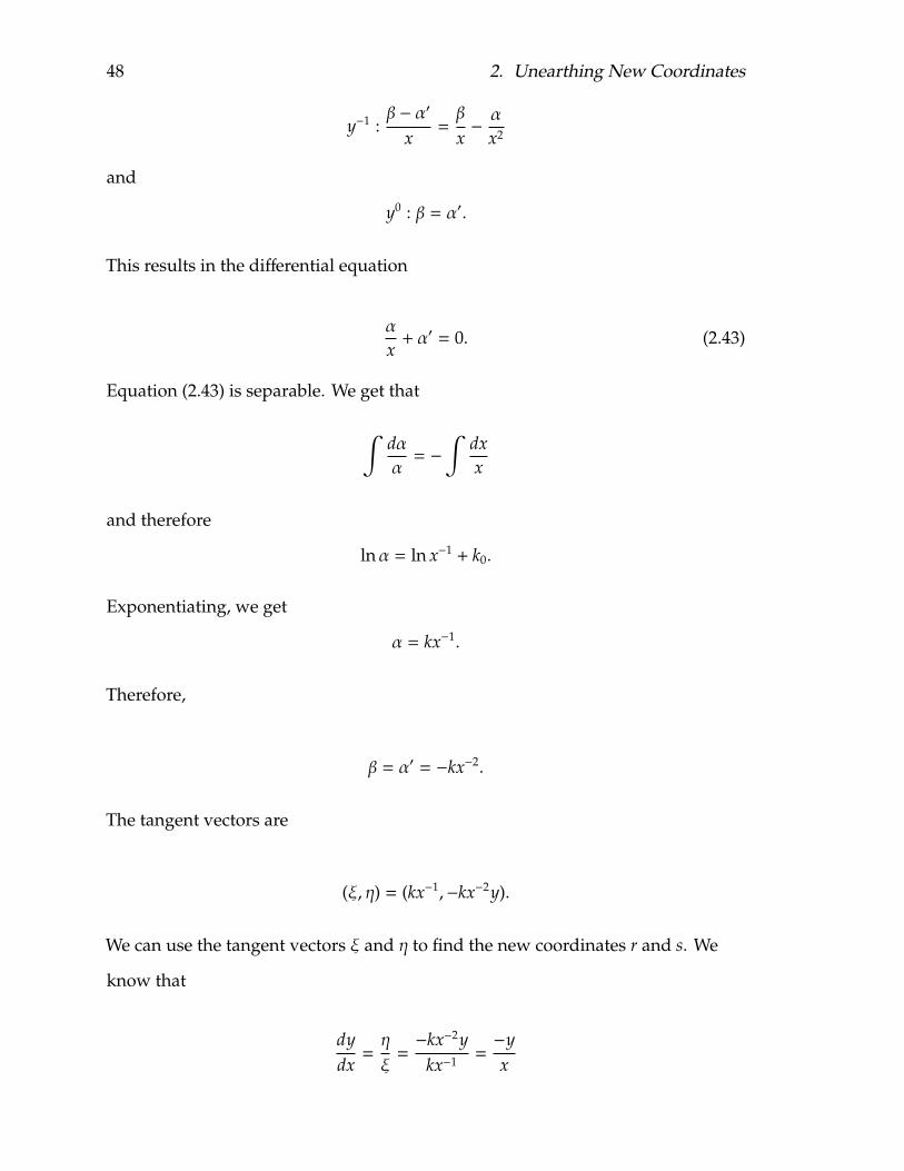
48 2. Unearthing New Coordinates
y−1 :β − α′
x=β
x− α
x2
and
y0 : β = α′.
This results in the differential equation
αx+ α′ = 0. (2.43)
Equation (2.43) is separable. We get that
∫dαα= −∫
dxx
and therefore
lnα = ln x−1 + k0.
Exponentiating, we get
α = kx−1.
Therefore,
β = α′ = −kx−2.
The tangent vectors are
(ξ, η) = (kx−1,−kx−2y).
We can use the tangent vectors ξ and η to find the new coordinates r and s. We
know that
dydx=ηξ=−kx−2y
kx−1 =−yx

2.4. The Linearized Symmetry Condition 49
Integrating, we get
ln y = − ln x + c0
and
y =cx.
Therefore
r = c = xy.
We can also find s:
s =∫
dxξ=
∫xdx =
12
x2.
The new coordinates are
(r, s) =(xy,
12
x2).
Solving these for x and y, we get x =√
2s and y = r√2s
.
To get the differential equation written in the new coordinates, we will use the total
derivative operator:
dsdr=
sx + ωsy
rx + ωry
=x
y + ( 1−y2+xyxy )x
=xy
1 + xy.
Substituting in x =√
2s and y = r√2s
yields the following result:
dsdr=
r1 + r
= 1 − 1r + 1
.
50 2. Unearthing New Coordinates
When we integrate this, we get
s =∫
1dr −∫
11 + r
= r − ln(1 + r).
Substituting s = 12x2 and r = xy, we find that the solution to Equation (2.39) is
12
x2 = xy − ln(1 + xy).
In this chapter, we have seen several examples illustrating how to find and use a
canonical coordinate system to solve first order differential equations. In the next
chapter, we will explore another tool, one that is useful for working with higher
order differential equations.
CHAPTER 3
Infinitesimal Generators
The material presented in this chapter is adapted from Differential Equations: Their
Solution Using Symmetries by Hans Stephani [6] and from Symmetry Methods for
Differential Equations: A Beginner’s Guide by Peter Hydon [2].
3.1 Infinitesimal Generator
The method described in Chapters 1 and 2 can be used to solve first order
differential equations. Many higher order differential equations can be reduced in
order with the use of infinitesimal generators [2]. For a one parameter Lie
symmetry group Pλ : (x, y) #→ (x, y) there exists the tangent vectors dxdλ |λ=0 = ξ(x, y)
and dydλ |λ=0 = η(x, y). The infinitesimal generator for the symmetry is the partial
differential operator
X = ξ∂∂x+ η∂∂y. (3.1)
Example 3.1.1. The following symmetry:
(x, y) = (x + λ, y + λ)
has an infinitesimal generator
X =∂∂x+∂∂y
51

52 3. Infinitesimal Generators
because ξ(x, y) = 1 and η(x, y) = 1.
Example 3.1.2. Consider the symmetry:
(x, y) =(
x1 − λy
,y
1 − λy
).
It has the tangent vectors
ξ(x, y) = xy
and
η(x, y) = y2.
The infinitesimal generator for this symmetry is
X = xy∂∂x+ y2 ∂∂y.
In most cases, it is not necessary to determine the symmetry based on the
infinitesimal generator. However, symmetries can be reconstructed from the
infinitesimal generators.
Example 3.1.3. Consider the following infinitesimal generator:
X =∂∂x+ y∂∂y. (3.2)
We can see that the tangent vectors are
ξ(x, y) = 1
and
η(x, y) = y.
Remember that ξ(x, y) is the derivative of x with respect to λ, evaluated at λ = 0.
3.1. Infinitesimal Generator 53
Similarly, η(x, y) is the derivative of y with respect to λ, evaluated at λ = 0. In this
example, ξ(x, y) = 1 so we could say that
ξ(x, y) = 1.
One equation for x that satisfies ξ(x, y) = 1 is
x = x + λ.
Because η(x, y) = y, one possible equation for η(x, y) is:
η(x, y) = eλy
and y can be written as
y = eλy.
Therefore, the symmetry corresponding to this infinitesimal generator is
(x, y) = (x + λ, eλy).
Other possibilities exist for symmetries that satisfy Equation (3.2). For example,
(x, y) = (2x + λ, eλy) would also satisfy (3.2).
The next example is more challenging. In the previous example, we can determine
the symmetries simply by looking at ξ(x, y) and η(x, y). This is not obvious in the
following example. One must use ξ(x, y) and η(x, y) to find the canonical
coordinates. Using the canonical coordinates, one can reconstruct the symmetry by
the method described in Section 2.2.
Example 3.1.4. We will reconstruct the symmetry that corresponds to the following
54 3. Infinitesimal Generators
infinitesimal generator:
X = (1 + x2)∂∂x+ xy
∂∂y. (3.3)
We know that ξ(x, y) = 1 + x2 and η(x, y) = xy. Now one can find the canonical
coordinates. To find r(x, y), solve
dydx=ηξ=
xy1 + x2 .
We getdyy=
xdx1 + x2 .
To integrate, it is necessary to do a u-substitution:
u = 1 + x2
and
du = 2x.
Now we can solve ∫dyy=
12
∫duu
to get
ln y =12
ln u + c.
This becomes
ln y = ln√
1 + x2 + c0.
When we exponentiate both sides, we get
y = c√
1 + x2.
3.1. Infinitesimal Generator 55
And then we can solve for r:
r =y√
1 + x2.
Now one can determine s using:
ds =dxξ(x, y)
,
and therefore
s =∫
dx1 + x2 .
Integrating, we get
s = arctan x + c.
We can solve r(x, y) and s(x, y) for x and y:
x = tan s
and
y = r√
1 + tan2 s.
Now we use the following equations from Section 2.2, Equations (2.24) and (2.25):
x = f (r, s) = f (r(x, y), s(x, y) + λ)
y = g(r, s) = g(r(x, y), s(x, y) + λ).
For this generator, Equation (3.3), x looks like:
x = tan s = tan(s + λ) = tan((arctan x) + λ).
Here, it can be shown that the addition formula for tan(a + b) is (Stewart front
56 3. Infinitesimal Generators
cover!):
tan(a + b) =tan a + tan b
1 − tan a tan b. (3.4)
Therefore,
x =x + sinλ
cosλ
1 − x(
sinλcosλ
) .
We can simplify this fraction to get
x =x cosλ + sinλcosλ − x sinλ
.
Similarly, we can find y using Equation (2.25):
y = r√
1 + tan2 s
= r√
1 + tan2(s + λ)
=y√
1 + x2·√
1 + tan2(arctan x + λ).
Now we will use Equation (3.4) to simplify this fraction:
y =y√
1 + x2·
√
1 +( x + tanλ1 − x tanλ
)2.
When we expand and simplify, we get
y =y√
1 + x2·√
1 + x2 tan2 λ + x2 + tan2 λ1 − 2x tanλ + x2 tan2 λ
= y ·√
(1 + x2)(1 + tan2 λ)(1 + x2)(1 − x tanλ)2 =
y√
1 + tan2 λ1 − x tanλ
=y√
1 + sin2 λcos2 λ
1 − x(
sinλcosλ
) =y√
1cos2 λ
cosλ−x sinλcosλ
.
3.2. Infinitesimal Generator in Canonical Coordinates 57
Therefore
y =y
cosλ − x sinλ.
And the symmetry is
(x, y) =(x cosλ + sinλcosλ − x sinλ
,y
cosλ − x sinλ
).
3.2 Infinitesimal Generator in Canonical
Coordinates
The infinitesimal generator can be written in the coordinates (u(x, y)) and (v(x, y)).
Let F(u, v) be an arbitrary smooth function. The infinitesimal generator acts on F:
XF(u, v) = XF(u(x, y), v(x, y)).
By the chain rule, we get
X = ξ(uxFu + vxFv) + η(uyFu + vyFv).
Simplifying this, we get
X = Fu(ξux + ηuy) + Fv(ξvx + ηvy).
Therefore
X = XuFu + XvFv.
58 3. Infinitesimal Generators
We know that F is an arbitrary function, so the infinitesimal generator in the
coordinates u(x, y) and v(x, y) is
X = Xu∂∂u+ Xv
∂∂v. (3.5)
Now consider the infinitesimal generator for the canonical coordinates r and s.
From Equation (3.5) we get
X = (Xr)∂∂r+ (Xs)
∂∂s
(3.6)
and
Xr = ξ(x, y)drdx+ η(x, y)
drdy.
This is Equation (2.10), which we have already dealt with in Chapter 2. Therefore,
we know that Xr = 0.
Similarly, from Equation (2.11) we get:
Xs = ξ(x, y)dsdx+ η(x, y)
dsdy,
which we have already dealt with in Chapter 2. Therefore, we know that Xs = 1.
Therefore, we know that Equation (3.6) is
X =∂∂s
in the canonical coordinates r(x, y) and s(x, y).
Infinitesimal generators make it possible to characterize the action of Lie
symmetries on functions without using canonical coordinates. This means that they
3.2. Infinitesimal Generator in Canonical Coordinates 59
can be extended to equations with more variables. First consider the situation in
two variables:
F(x, y) = G(r(x, y), s(x, y))
and therefore
F(x, y) = G(r, s) = G(r, s + λ).
We can expand this using the Taylor Series. At first glance, this seems to be a two
variable problem, but we know from Equation (2.10) that Xr = 0. The derivative
operator on r is 0. We also know that r = r. Now consider the Taylor Series for
F(x, y) = G(r, s) centered at s:
F(x, y) = G(r, s) + Gs(r, s)(s + λ − s) +Gss(r, s)
2!(s + λ − s)2 +
Gsss(r, s)3!
(s + λ − s)3 + ...
=∞∑
j=0
λ j
j!∂ j
∂sj G(r, s).
Because X = ∂∂s in the canonical coordinates r(x, y) and s(x, y), we can write:
F(x, y) =∞∑
j=0
λ j
j!XjG(r, s).
We know that G(r, s) = F(x, y) so
F(x, y) =∞∑
j=0
λ j
j!XjF(x, y). (3.7)
We know that the Taylor series expansion for ex is
ex =∞∑
j−0
xj
j!.
60 3. Infinitesimal Generators
Therefore, Equation (3.7) can be rewritten as
F(x, y) = eλXF(x, y). (3.8)
This notation is useful for studying the symmetries associated with higher order
differential equations [2].
The information in this chapter can be expanded to any number of variables.
Suppose a function has L variables, z1, z2, ..., zL. Then, the Taylor expansion for zs is
zs(z1, z2, ...zL;λ) = zs + λζs(z1, ...zL) +O(λ2)
where
ζs =dzs
dλ|λ=0.
The infinitesimal generator is
X = ζs(z1, z2, ..., zL)∂∂zs .
The material presented in this chapter can be used with higher order differential
equations. We will see a preliminary example in the next chapter.

CHAPTER 4
Higher Order Differential Equations
This chapter will extend the use of the infinitesimal generator for higher order
differential equations. The material presented in this chapter comes from Symmetry
Methods for Differential Equations: A Beginner’s Guide by Peter Hydon [2] and from
Differential Equations: Their Solutions Using Symmetries by Hans Stephani [6].
4.1 The Symmetry Condition for Higher Order
Differential Equations
In this chapter we will consider higher order differential equations of the form
y(k) = ω(x, y, y′, ..., y(k−1)). (4.1)
Symmetries for higher order differential equations work similarly to symmetries for
first order differential equations. The symmetry must map one solution curve to
another. The mapping takes x to x, y to y, y′ to y′ and so forth, where y(k) is defined
as
y(k) =dkydxk . (4.2)
The kth derivative of y is calculated recursively. Remember that the kth derivative of
61

62 4. Higher Order Differential Equations
y is the derivative of the (k − 1)st derivative of y. Therefore
yk =dy(k−1)
dx=
Dxy(k−1)
Dxx. (4.3)
The symmetry condition for first order differential equations requires that a
mapping P : (x, y) #→ (x, y) take one solution curve to another. Thus the symmetry
condition for a first order differential equation is
dydx= ω(x, y). (4.4)
It works in the same fashion for higher order differential equations- a mapping
takes a solution curve to another solution curve. Therefore, the symmetry condition
for higher order differential equations is
dnydxn = y(n) = ω(x, y, y′, ..., y(n−1)). (4.5)
The following example demonstrates how to verify the symmetry condition, and
demonstrates how to compute y(k).
Example 4.1.1. Consider the following differential equation:
y′′ = 0. (4.6)
In this example, we will verify that the following symmetry holds for Equation (4.6):
(x, y) =(1x,
yx
).
In other words, we will show that y′′ = 0 under this symmetry. In order to calculate
y′′, we must first calculate y′ using y and x. To begin, we take the partial
4.1. The Symmetry Condition for Higher Order Differential Equations 63
derivatives of y and x in order to take the total derivative operator:
yx =−yx2 , yy =
1x
and
xx =−1x2 , xy = 0.
Then we can use Equation (4.3) to find y′:
y′ =dydx=
Dx
( yx
)
Dx
(1x
)
=
−yx2 +
y′
x−1x2
= y − y′x.
Then we can use Equation (4.3) and y′ to find y′′, thus verifying that y′′ is equal to 0:
y′′ =dy′
dx=
Dx(y − y′x)Dx( 1
x )
= (−y′ + y′ + y′′(−x))(−x2) = x3y′′.
Therefore, the symmetry condition is satisfied because y′′ = 0. We have just shown
that y′′ = 0.
The symmetry (x, y) =(
1x ,
yx
)for Equation (4.6) is actually a discrete symmetry,
rather than a continuous symmetry. The general solution to y′′ = 0 is
y = c1x + c2.
When one applies the symmetry, the result is
y = c1x + c2,

64 4. Higher Order Differential Equations
and thereforeyx=
c1
x+ c2.
When we multiply by x we get
y = c1 + c2x.
This symmetry is its own inverse. Applied once, it maps to y = c1 + c2x. Applied a
second time, it maps back to y = c1x + c2.
4.2 The Linearized Symmetry Condition, Revisited
In Section 2.4, we worked with the linearized symmetry condition for first order
differential equations. One can use the linearized symmetry condition to determine
the tangent vectors ξ(x, y) and η(x, y). Similarly, one can use a linearized symmetry
condition for higher order differential equations as well. As demonstrated in the
next example, the linearized symmetry condition can be used to find the
infinitesimal generator for a given symmetry. First we will demonstrate how to find
the linearized symmetry condition for higher order differential equations. To begin,
here are the Taylor series expansions for x, y, and y(k):
x = x + λξ +O(λ2), (4.7)
y = y + λη +O(λ2), (4.8)
y(k) = y(k) + λ(
(k)η)+O(λ2). (4.9)
Here, (k)η denotes the tangent vector that corresponds to the kth derivative of y [6]:
(k)η =∂y(k)
∂λ
∣∣∣∣∣λ=0.
4.2. The Linearized Symmetry Condition, Revisited 65
If we substitute Equations (4.7), (4.8), and (4.9) into Equation (4.5), we get
y(n) = ω(x + λξ +O(λ2), y + λη +O(λ2), y′ + λ′η +O(λ2), ...y(n−1) + λ(
(n−1)η)+O(λ2)).
(4.10)
Using the chain rule to take the derivative of Equation (4.10) with respect to λ
(evaluated at λ = 0), we get the linearized symmetry condition:
(n)η = ξωx + ηωy +(
(1)η)ωy(1) + ... +
((n−1)η
)ωy(n−1) . (4.11)
We can calculate (n)η recursively. Consider, (1)η. By definition:
y′ =DxyDxx.
First compute Dxy using the Taylor series expansion of y:
Dxy = ληx + y′(1 + ληy) +O(λ2)
= y′ + ληx + λy′ηy
= y′ + λDxη +O(λ2).
Then compute Dxx using the Taylor series expansion of x:
Dxx = 1 + λξx + y′(λξy)
= 1 + λDxξ +O(λ2).
Therefore
y′ =DxyDxx
=y′ + λDxη +O(λ2)1 + λDxξ +O(λ2)
. (4.12)

66 4. Higher Order Differential Equations
Now multiply Equation (4.12) by
1 − λDxξ1 − λDxξ
and ignore terms of λ2 or higher, as we did while calculating the linearized
symmetry condition for first order differential equations in Section 2.4. We get:
y′ = (y′ + λDxη)(1 − λDxξ) +O(λ2)
= y′ + λ(Dxη − y′Dxξ) +O(λ2).
When we compare this with Equation (4.9), we find that
(1)η = Dxη − y′Dxξ.
We can generalize this for (k)η. From Equation (4.3), we know that
y(k) =Dxy(k−1)
Dxx.
We have already computed Dxx. Now we will compute Dxy(k−1). First remember
that
y(k−1) = y(k−1) + λ(
(k−1)η)+O(λ2).
Therefore,
Dxy(k−1) = λ(
(k−1)ηx
)+ y′λ
((k−1)ηy
)+ y′′λ
((k−1)ηy′
)+ ... + y(k)
(1 + λ
((k−1)ηy(k−1)
))+O(λ2)
= y(k) + λ(
(k−1)ηx
)+ y′λ
((k−1)ηy
)+ y′′λ
((k−1)ηy′
)+ ... + y(k)λ
((k−1)ηy(k−1)
)O(λ2)
= y(k) + λDx
((k−1)η
)+O(λ2).

4.2. The Linearized Symmetry Condition, Revisited 67
Thus,
y(k) =Dxy(k−1)
Dxx(4.13)
=y(k) + λDx
((k−1)η
)+O(λ2)
1 + λDxξ +O(λ2). (4.14)
When we multiply Equation (4.13) by
1 − λDxξ1 − λDxξ
we get
y(k) = y(k) − y(k)λDxξ + λD(k−1)x η +O(λ2)
= y(k) + λ(D(k−1)x η − y(k)Dxξ) +O(λ2).
Comparing this result with Equation (4.9), we get
(k)η = D(k−1)x η − y(k)Dxξ. (4.15)
As k increases, the number of terms in (k)η increases exponentially [2]. For this
reason, we will only compute (1)η and (2)η in this IS. The computation for (1)η goes as
follows:
(1)η = ηx + ηy(y′) − y′(ξx + ξyy′)
= ηx + ηyy′ − y′ξx − ξy(y′)2
= ηx + y′(ηy − ξx) − ξy(y′)2.

68 4. Higher Order Differential Equations
And then we can use (1)η to compute (2)η:
(2)η = D(1)x η − y′′Dxξ
= ηxx + y′ηyx − y′ξxx − ξyx(y′)2 + y′(ηxy + y′ηyy − y′ξxy − ξyy(y′)2)
+ y′′(ηy − ξx − 2ξyy′) − y′′(ξx + ξyy′)
= ηxx + y′(2ηxy − ξxx) + (y′)2(ηyy − 2ξxy) − ξyy(y′)3 + (ηy − 2ξx − 3ξyy′)y′′
Substituting (2)η into Equation (4.11), we find that the the linearized symmetry
condition for second order differential equations is
(2)η = ηxx + y′(2ηxy − ξxx) + (y′)2(ηyy − 2ξxy) − ξyy(y′)3 + (ηy − 2ξx − 3ξyy′)y′′
= ξωx + ηωy +(1) ηωy′ . (4.16)
We will use Equation (4.16) to determine the infinitesimal generator for the
following example.
Example 4.2.1. Again, consider the following second order differential equation:
y′′ = 0. (4.17)
Because y′′ = ω(x, y) = 0, we know that (2)η = 0. That leaves us with:
ηxx + y′(2ηxy − ξxx) + (y′)2(ηyy − 2ξxy) − ξyy(y′)3 = 0. (4.18)
Equation (4.18) can be split into a system of four equations, called the determining
equations:
ηxx = 0 (4.19)
2ηxy − ξxx = 0 (4.20)

4.2. The Linearized Symmetry Condition, Revisited 69
ηyy − 2ξxy = 0 (4.21)
and
ξyy = 0. (4.22)
Integrating Equation (4.22) with respect to y twice results in
ξ(x, y) = A(x)y + B(x).
Then substitute ξ(x, y) into Equation (4.21):
ηyy = 2A′(x). (4.23)
When we integrate Equation (4.23) with respect to y, we get
ηy = 2A′(x)y + C(x).
Then integrate with respect to y again to get:
η(x, y) = A′(x)y2 + C(x)y +D(x).
Now we can substitute ξ(x, y) and η(x, y) into Equations (4.20) and (4.19). First, we
must compute ηxy, ξxx, and ηxx:
ηxy = 2A′′(x)y + C′(x)
ξxx = A′′(x)y + B′′(x)
and
ηxx = A′′′(x)y2 + C′′(x)y +D′′(x) = 0. (4.24)
70 4. Higher Order Differential Equations
Therefore, Equation (4.20) yields:
2ηxy − ξxx = 2(2A′′(x)y + C′(x)) − (A′′(x)y + B′′(x)) (4.25)
= 3A′′′(x)y + 2C′(x) − B′′(x) = 0.
From Equations (4.24) and (4.25), we can determine that A′′(x) = 0, C′′(x) = 0,
D′′(x) = 0 and B′′(x) = 2C′(x). The general solutions for A(x), B(x), and C(x) are
A(x) = c1x + c2
C(x) = c3x + c4
and
D(x) = c5x + c6
where c1, c2, c3, c4, c5, and c6 are constants. We can solve for B(x):
B′′(x) = 2C′(x) = 2c3
B′(x) = 2c3x + c7
B(x) = c3x2 + c7x + c8.
When we substitute A(x), B(x), C(x), and D(x) back into ξ(x, y) and η(x, y), we get:
ξ(x, y) = A(x)y + B(x)
= c1xy + c2y + c3x2 + c7x + c8
4.2. The Linearized Symmetry Condition, Revisited 71
and
η(x, y) = A′(x)y2 + C(x)y +D(x)
= c1y2 + c3xy + c4y + c5x + c6.
Therefore, the infinitesimal generator for y′′ = 0 is:
X = (c1xy + c2y + c3x2 + c7x + c8)∂x + (c1y2 + c3xy + c4y + c5x + c6)∂y.
In this chapter, we have illustrated how symmetry methods for higher order
equations work with one example - the simplest 2nd order differential equation,
y′′ = 0. There are numerous possibilities for using symmetry methods to solve
higher order differential equations or to obtain a reduction in order. Several
resources for further study of symmetry methods are presented in the conclusion
chapter.

72 4. Higher Order Differential Equations
CHAPTER 5
Conclusion
This Independent Study has demonstrated just a small portion of the possibilities
for using Lie symmetry groups to solve differential equations. Chapters 1 and 2
explained the fundamentals of this method for first order ODEs, while Chapters 3
and 4 described some of the tools necessary to extend the work in Chapters 1 and 2
to higher order differential equations. These tools have applications in a variety of
disciplines.
We have only explored a small sampling of the resources available for studying Lie
symmetry methods. The main sources for this I.S. offer several more chapters of
information pertaining to these methods. Hydon’s, Symmetry Methods for
Differential Equations: A Beginner’s Guide explains how to use Lie symmetries with
several parameters and also includes methods for solving partial differential
equations (PDEs) [2]. Stephani’s Differential Equations: Their Solution Using
Symmetries offers a detailed explanation of symmetry methods for both ODEs and
PDEs. Stephani also includes a chapter on solving systems of differential equations
[6]. Ibragimov’s Elementary Lie Group Analysis and Ordinary Differential Equations is
another highly relevant resource for anyone wishing to study the applications of
Lie symmetry methods and other tools for solving differential equations [3]. This
book has a wealth of information on the application of these methods to physics
and engineering.
73
74 5. Conclusion
This project proved challenging in a variety of ways. The selection of the topic
resulted from a desire to utilize knowledge from multiple mathematics courses at
The College of Wooster, particularly Abstract Algebra and Differential Equations.
Basic comprehension of the mathematics involved took a significant amount of
time and dedication. Starrett’s “Solving Differential Equations by Symmetry
Groups" provided a basis for understand the fundamental techniques of Lie
symmetry methods [5]. His explanations and examples became useful for further
study and for learning the first two chapters of Hydon. Much of this I.S. combines
these two sources.
The challenge acquired a new dimension in November, when writing commenced.
Some difficulty stemmed from communicating the mathematics clearly and
effectively while adhering to the constraints of mathematical and scientific writing.
In addition, incorporating equations into proper English prose seemed
unexpectedly difficult. This resulted in a number of period placement catastrophes
in primitive drafts of Chapter 2.
Finishing this project required skills not only from several math classes but also
from quite a few other Wooster classes. This included everything from outlining
methods learned in First Year Seminar to drafting strategies developed in writing
intensive courses to stress management techniques (and increased familiarity with
the Greek alphabet!) acquired during study abroad. Overall, the scope of this
project has made it a fitting conclusion to my Wooster career.
References
1. R.L. Burden and J.D. Faires, Numerical analysis, Brooks/Cole, 2011.
2. Peter E. Hydon, Symmetry methods for differential equations, Cambridge Texts inApplied Mathematics, Cambridge University Press, Cambridge, 2000, Abeginner’s guide. MR 1741548 (2001c:58036)
3. Nail H. Ibragimov, Elementary Lie group analysis and ordinary differential equations,Wiley Series in Mathematical Methods in Practice, vol. 4, John Wiley & Sons Ltd.,Chichester, 1999. MR 1679646 (2000f:34007)
4. D. Poole, Linear algebra: A modern introduction, Available 2011 Titles EnhancedWeb Assign Series, Brooks/Cole, 2010.
5. John Starrett, Solving differential equations by symmetry groups, Amer. Math.Monthly 114 (2007), no. 9, 778–792. MR 2360906 (2008i:34072)
6. Hans Stephani, Differential equations, Cambridge University Press, Cambridge,1989, Their solution using symmetries. MR 1041800 (91a:58001)
7. J. Stewart, Calculus, Stewart’s Calculus Series, Brooks/Cole, 2008.
8. D.G. Zill, A first course in differential equations: With modeling applications,Brooks/Cole, 2008.
75


![Truth About a Lie (v2) [English]](https://img.pdfslide.net/doc/110x75/577cdddc1a28ab9e78adeaa4/truth-about-a-lie-v2-english.jpg)