Embed Size (px)
Citation preview
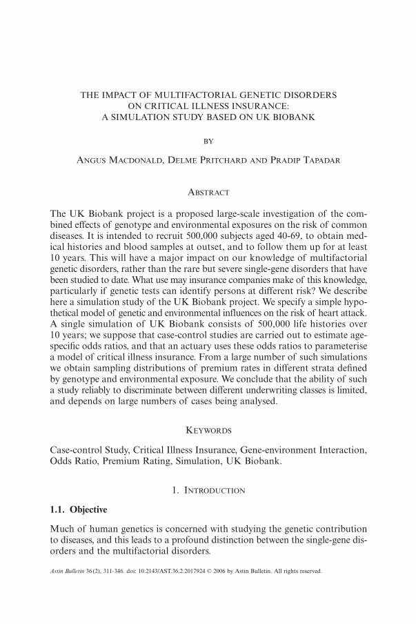
THE IMPACT OF MULTIFACTORIAL GENETIC DISORDERSON CRITICAL ILLNESS INSURANCE:
A SIMULATION STUDY BASED ON UK BIOBANK
BY
ANGUS MACDONALD, DELME PRITCHARD AND PRADIP TAPADAR
ABSTRACT
The UK Biobank project is a proposed large-scale investigation of the com-bined effects of genotype and environmental exposures on the risk of commondiseases. It is intended to recruit 500,000 subjects aged 40-69, to obtain med-ical histories and blood samples at outset, and to follow them up for at least10 years. This will have a major impact on our knowledge of multifactorialgenetic disorders, rather than the rare but severe single-gene disorders that havebeen studied to date. What use may insurance companies make of this knowledge,particularly if genetic tests can identify persons at different risk? We describehere a simulation study of the UK Biobank project. We specify a simple hypo-thetical model of genetic and environmental influences on the risk of heart attack.A single simulation of UK Biobank consists of 500,000 life histories over10 years; we suppose that case-control studies are carried out to estimate age-specific odds ratios, and that an actuary uses these odds ratios to parameterisea model of critical illness insurance. From a large number of such simulationswe obtain sampling distributions of premium rates in different strata definedby genotype and environmental exposure. We conclude that the ability of sucha study reliably to discriminate between different underwriting classes is limited,and depends on large numbers of cases being analysed.
KEYWORDS
Case-control Study, Critical Illness Insurance, Gene-environment Interaction,Odds Ratio, Premium Rating, Simulation, UK Biobank.
1. INTRODUCTION
1.1. Objective
Much of human genetics is concerned with studying the genetic contributionto diseases, and this leads to a profound distinction between the single-gene dis-orders and the multifactorial disorders.
Astin Bulletin 36 (2), 311-346. doi: 10.2143/AST.36.2.2017924 © 2006 by Astin Bulletin. All rights reserved.
9130-06_Astin_36/2_01 06-12-2006 11:52 Pagina 311
(a) Single-gene disorders are caused, as their name suggests, by a defect in asingle gene. Because most genes are inherited in a simple way accordingto Mendel’s laws, these diseases show characteristic patterns of inheritancefrom one generation to the next, known to geneticists and underwriters alikeas a ‘family history’. Single-gene disorders are quite rare but often severe.
(b) Multifactorial disorders are (mostly) common diseases, such as coronaryheart disease and cancers, whose onset or progression may be influencedby variations in several genes, acting in concert with environmental differ-ences. The effect is likely to be quite slight, conferring an altered predis-position to the disease rather than a radically different risk.
Most genetic epidemiology has, until now, concentrated on single-gene disorders.One reason is that the clear patterns of Mendelian inheritance identifiedaffected families long before molecular genetics came along. When these toolsemerged in the 1990s, geneticists knew where to look; affected families werestudied, genes were identified, and the key epidemiological parameters were esti-mated. The parameter of most interest to actuaries is the age-related pene-trance, which is the probability that a person who carries a risky version of thegene will have suffered onset of the disease by age x. It is entirely analogousto the life table probability xq0. (Often, the risky versions of the gene are called‘mutations’, and a person carrying one is called a ‘mutation carrier’ or just‘carrier’.)
Studies of affected families are by definition retrospective; families arestudied because they are known to be affected. This introduces uncontrolled sourcesof bias, so such studies are, if possible, avoided in favour of prospective studies,in which a properly randomised sample of healthy subjects is followed forwardsin time. Despite this health warning, retrospective studies of single-gene dis-orders have been carried out for reasons of convenience, cost and necessity:the ready availability of known affected families was convenient and madedata collection relatively cheap; and the rarity of single-gene disorders madeprospective studies impractical. Moreover, a prospective study would take manyyears to yield results. Another consequence of the rarity of most single-genedisorders is that most studies have had quite small sample sizes, but if the pen-etrance is high enough this is tolerable. These studies have successfully led tomany gene discoveries and a lot of progress has been made in understandingsingle-gene disorders.
Multifactorial disorders are not so well-studied, and are much harder tostudy. The clear patterns of Mendelian inheritance are lost, and any familialclustering of disease that may be observed could just as easily be the result ofshared environment as of shared genes. Therefore, there is no pool of knownaffected families that can be studied straightaway. And, because the influenceof genetic variation may be slight (low penetrance) large samples will be neededto detect such influence with any reliability.
At the risk of oversimplifying a little, single-gene disorders represent the genet-ical research of the past, and multifactorial disorders represent the genetical
312 A. MACDONALD, D. PRITCHARD AND P. TAPADAR
9130-06_Astin_36/2_01 06-12-2006 11:52 Pagina 312
research of the future. Progress will need studies that are large-scale, prospec-tive, and long-term (therefore very expensive) and that capture both genetic andenvironmental variation and the incidence of common diseases. This is veryambitious.
The proposed UK Biobank project aims to achieve this. UK Biobank willrecruit 500,000 individuals aged 40 to 69, chosen as randomly as possible fromthe UK population, and collect data on them over 10 years. We will discussits main features in Section 1.2. A key point is that UK Biobank aims only tocollect data, not to analyse it. Its data will, in due course, be made availableto researchers interested in particular genes and particular diseases, who willhave to obtain separate funding for their studies. This is sensible because it isimpossible to predict at outset just what combinations of genes, environment anddisease it will be most fruitful to study. Nevertheless, it is necessary to have inmind the kinds of statistical studies most likely to be carried out, so that UKBiobank can be set up to capture data of the correct form. The presumption isthat most studies will be case-control studies. We outline these in the Appendix.
Given its size and significance, it is important to study the kind of resultswe might expect to emerge out of UK Biobank. Our particular interest is inthe implications of UK Biobank for insurance. We need not rehearse the debate,often heated, that has surrounded genetics and insurance in the past 10 years,except to note that it has mainly focussed on single-gene disorders. Daykin et al.(2003) or Macdonald (2004) are sources. It seems plausible that awareness ofgenetic issues will be heightened by enrolling 500,000 people into a genetic study.If insurance questions arise, answers obtained from past actuarial researchinto single-gene disorders may be wholly inapplicable. But, since the single-gene disorders provide all the easily grasped examples and paradigms, there isa risk that these examples and paradigms will be grafted onto UK Biobank,however inappropriately, by the media if not by the genetics community. It willthen be unfortunate that UK Biobank will not provide the evidence to refutesuch errors for 5-10 years.
Our plan, therefore, is to model UK Biobank itself, so that before a singleperson has been recruited, or gene sequenced, we may quantify the implicationsof its outcomes for insurance. We choose critical illness (CI) insurance as thesimplest type of coverage, because the insured event is generally disease onset.We choose heart attack (myocardial infarction) as the disease of interest,because this will certainly be a major target of studies using UK Biobank data.Our approach is simple: simulate 500,000 random life histories, given an assumedmodel of genetic and environmental influences on the hazard rate of heartattack. Then we may analyse these simulated data just as an epidemiologist oran actuary may be expected to.
At this stage a further complication appears, very familiar to actuarialresearchers who have modelled single-gene disorders. Actuaries almost never haveaccess to the original data upon which genetic studies are based. Section 5.2 ofthe UK Biobank draft protocol (www.ukbiobank.ac.uk/docs/draft/protocol.pdf)says: ‘‘Data from the project will not be accessible to the insurance industry
THE IMPACT OF GENETIC DISORDERS ON CRITICAL ILLNESS INSURANCE 313
9130-06_Astin_36/2_01 06-12-2006 11:52 Pagina 313
or any other similar body.’’ This means that actuarial researchers will have to relyon the published outcomes of medical or epidemiological research projects thatuse the UK Biobank data, in particular case-control studies. The ideal, giventhe models actuaries typically use for pricing and reserving, would be age-dependent onset rates or penetrances, corresponding to mx or qx in a life table.Unfortunately, this far exceeds what is usually published, because the questionsasked in a medical study can often be answered by much simpler statistics. And,it must be said, the estimation of mx or qx is very demanding of the data. So wemay not, realistically, assume that the actuary can analyse directly the 500,000simulated life histories. Instead, an epidemiologist must first carry out a case-control study and publish the results, probably in the form of odds ratios (seethe Appendix). Then the actuary must take these odds ratios and, using what-ever approximate methods come to hand, estimate onset rates or penetrances suit-able for use in an actuarial model. We will model this process, with two results:
(a) We will be able to estimate the impact on CI insurance premiums of rep-resentative multifactorial modifiers of heart attack risk.
(b) Having simulated the data from a known model of our own choosing, wecan assess the seriousness of the errors that must be made, in parameter-ising an actuarial model from published odds ratios rather than from theraw data. As mentioned before, previous actuarial studies have done exactlythat (see Macdonald & Pritchard (2000) for an example), but only in thecontext of relatively high penetrances. We will be interested to see if robustactuarial modelling of relatively low-penetrance disorders is possible usingpublished case-control studies.
The plan of the paper is as follows. In the remainder of this section we describethe main features of UK Biobank and our general approach. A model repre-senting heart attack will be introduced and parameterised in Section 2, includinga simple hypothetical 2 ≈ 2 gene-environment interaction model affecting heartattack risk.
In Section 3, we present (in summary form) and analyse a set of simulatedUK Biobank data, namely 500,000 life histories. A model epidemiologist carriesout a case-control study, then our model actuary uses these ‘published’ figuresto find critical illness premium rates allowing for genetic variability and environ-mental exposures.
Despite its great size, UK Biobank is essentially an unrepeatable single sam-ple. Any estimated quantity based upon its data is subject to the usual sam-pling error — and a premium rate is just such an estimated quantity. We canassess directly the sampling properties of estimates based on UK Biobankdata, simply by repeating the simulation of 500,000 life histories as many timesas necessary, and constructing the empirical distributions of the odds ratios andpremium rates. This is in Section 4. This is directly relevant to the criteriaestablished in the UK by the Genetics and Insurance Committee (GAIC) forassessing the reliability of premium rates based on genetic information.
Conclusions and suggestions for further work are in Section 5.
314 A. MACDONALD, D. PRITCHARD AND P. TAPADAR
9130-06_Astin_36/2_01 06-12-2006 11:52 Pagina 314

1.2. The UK Biobank Project
The website http://www.ukbiobank.ac.uk/ is the main source of information on UKBiobank. In particular, it provides a draft protocol, which states (Section 1.2) that:
‘‘The main aim of the study is to collect data to enable the investigation of theseparate and combined effects of genetic and environmental factors (includinglifestyle, physiological and environmental exposures) on the risk of commonmultifactorial disorders of adult life.’’
UK Biobank is a cohort study, meaning that a large number of people will berecruited, as randomly as possible, and then followed over time. The main fea-tures of the study design are as follows:
(a) The cohort will consist of at least 500,000 men and women recruited fromthe UK general population.
(b) The chosen age range is 40 to 69 (note that earlier versions, including thedraft protocol referred to above, proposed an age range 45 to 69).
(c) The initial follow-up period is 10 years.(d) Participants will be recruited through their local general practitioners.
Participants are expected to come from a broad range of socio-economicbackgrounds and regions throughout the UK, with a wide range of exposuresto factors of interest.
(e) The project will be conducted through the UK National Health Service.(f) UK Biobank is funded by the Department of Health, the Medical Research
Council, the Scottish Executive and The Wellcome Trust, and will costapproximately £40 million.
People registered with participating general practices will be requested to jointhe study by completing a self-administered questionnaire, attending an inter-view, undergoing examination by a research nurse and giving a blood sample,to enable DNA extraction at a later date, as and when genotyping is required.
The Office of National Statistics will provide routine follow-up data regard-ing cause-specific mortality and cancer incidence. Hospitalisation and generalpractice records will provide data regarding incident morbidity. Every twoyears a subset of 2,000 participants and every five years the entire cohort willbe re-surveyed by postal questionnaire to update exposure data and to ascertainself-reported incident morbidity.
It is envisaged that the main study design for later analysis will be a case-control study (see the Appendix) nested within the cohort. UK Biobank willonly collect and store the data, its analysis will require further funding.
1.3. A UK Biobank Simulation Model
In this section we outline how we will simulate the UK Biobank project.
THE IMPACT OF GENETIC DISORDERS ON CRITICAL ILLNESS INSURANCE 315
9130-06_Astin_36/2_01 06-12-2006 11:52 Pagina 315
We suppose that the study population is subdivided (or stratified) into sub-groups with respect to: (a) genotype; (b) level of environmental exposure;and (c) other relevant factors such as sex. Genotype defines discrete categories,and we suppose that environmental exposures or other factors defined on acontinuous scale are grouped into discrete categories. Thus, we always have asmall number of discrete subgroups (or strata).
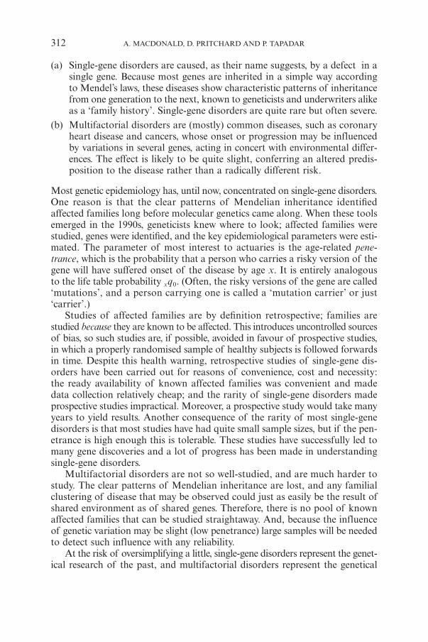
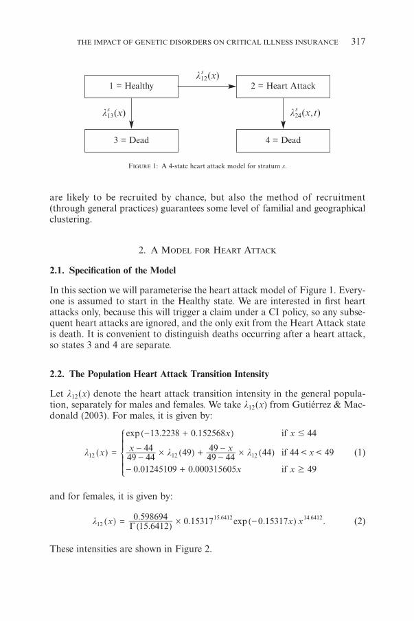
The life history of each participant, including the occurrence of a heart attack,will be represented by the multiple-state model shown in Figure 1. It is para-meterised by intensities denoted ls
ij (x) or lsij (x, t), functions of age x and pos-
sibly also duration t since entering state i. The superscript ‘s ’ indicates stratum,and the intensities representing heart attacks will be stratum-dependent. Theseintensities are the key to the whole UK Biobank project, as well as our study.
(a) The real-life epidemiologist wants to estimate them (or in practice, odds ratios)from UK Biobank data, given a hypothesis about the effect of measuredexposures on the disease.
(b) The real-life actuary wants to take the estimated intensities (or in practice,approximate them from published odds ratios) and use them in pricing andreserving.
(c) We want to specify hypothetical but plausible dependencies of these inten-sities on genotype and other exposures, so that we can observe our modelepidemiologist and model actuary at work.
1.4. Simulating UK Biobank
The steps in simulating UK Biobank are then as follows.
(a) We choose the number of genotypes and the number of levels of environ-mental exposure, and also the frequencies with which each appears in thepopulation. Thus we can model simple or complex genotypes and envi-ronmental exposures, and allow them to be more or less common or rare.These define the subgroups or strata. The simplest example (used in the UKBiobank draft protocol) is to have two genotypes and two levels of envi-ronmental exposure. We also choose the intensities of onset of heart attackin each stratum (ls
12(x) in Figure 1).
(b) We randomly ‘create’ 500,000 individuals, each equally likely to be maleor female, and with ages uniformly distributed in the range 40 to 70, andallocated to strata at random according to the chosen frequencies.
(c) The life history of each individual is modelled by simulating the times ofany transitions between states in the model, as governed by the intensities.We record the times of any transitions taking place within the 10-year fol-low-up period of UK Biobank.
We assume that the 500,000 participants are independent in the statistical sense,which is unlikely to be true. The sample is so large that some related individuals
316 A. MACDONALD, D. PRITCHARD AND P. TAPADAR
9130-06_Astin_36/2_01 06-12-2006 11:52 Pagina 316
are likely to be recruited by chance, but also the method of recruitment(through general practices) guarantees some level of familial and geographicalclustering.
2. A MODEL FOR HEART ATTACK
2.1. Specification of the Model
In this section we will parameterise the heart attack model of Figure 1. Every-one is assumed to start in the Healthy state. We are interested in first heartattacks only, because this will trigger a claim under a CI policy, so any subse-quent heart attacks are ignored, and the only exit from the Heart Attack stateis death. It is convenient to distinguish deaths occurring after a heart attack,so states 3 and 4 are separate.
2.2. The Population Heart Attack Transition Intensity
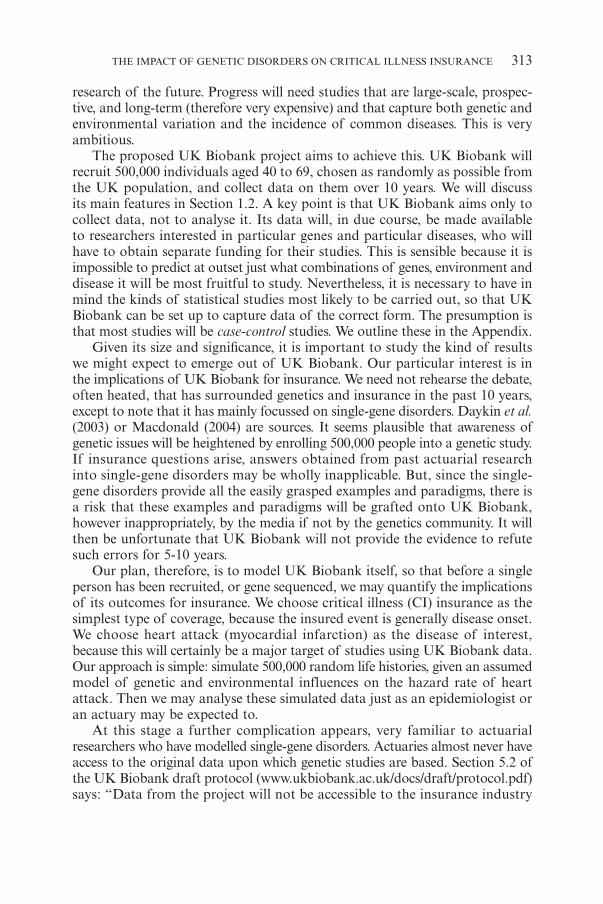
Let l12(x) denote the heart attack transition intensity in the general popula-tion, separately for males and females. We take l12(x) from Gutiérrez & Mac-donald (2003). For males, it is given by:
. .
< <
. .
exp
x
x x
x x x
x x
if
if
if
l l l
13 2238 0 152568 44
49 4444 49 49 44
49 44 44 49
0 01245109 0 000315605 49
12 12 12# #
#
$
=
- +
--
+--
- +
]
]
] ]g
g
g g
Z
[
\
]]
]]
(1)
and for females, it is given by:
.. . . .expx x xl G 15 6412
0 598694 0 15317 0 15317. .12
15 6412 14 6412#= -]
]]g
gg (2)
These intensities are shown in Figure 2.
THE IMPACT OF GENETIC DISORDERS ON CRITICAL ILLNESS INSURANCE 317
FIGURE 1: A 4-state heart attack model for stratum s.
1 = Healthy
3 = Dead
2 = Heart Attack
4 = Dead
ls24(x,t)ls
13(x)
ls12(x)
9130-06_Astin_36/2_01 06-12-2006 11:53 Pagina 317
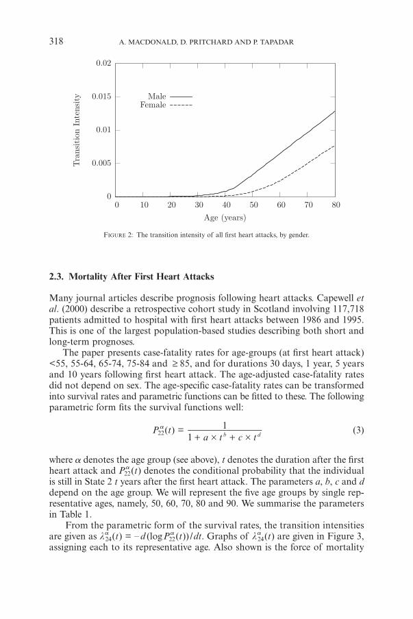
FIGURE 2: The transition intensity of all first heart attacks, by gender.
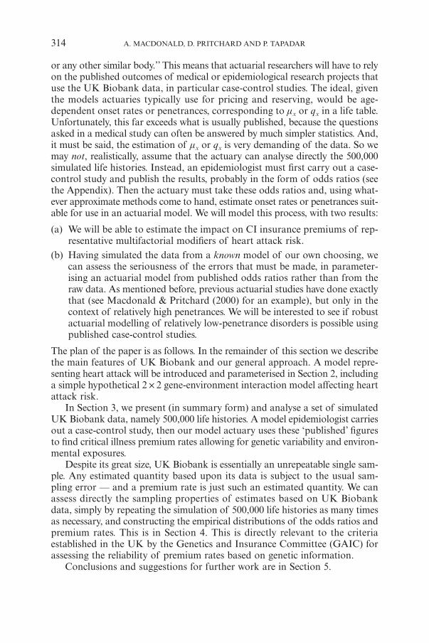
2.3. Mortality After First Heart Attacks
Many journal articles describe prognosis following heart attacks. Capewell etal. (2000) describe a retrospective cohort study in Scotland involving 117,718patients admitted to hospital with first heart attacks between 1986 and 1995.This is one of the largest population-based studies describing both short andlong-term prognoses.
The paper presents case-fatality rates for age-groups (at first heart attack)<55, 55-64, 65-74, 75-84 and ≥ 85, and for durations 30 days, 1 year, 5 yearsand 10 years following first heart attack. The age-adjusted case-fatality ratesdid not depend on sex. The age-specific case-fatality rates can be transformedinto survival rates and parametric functions can be fitted to these. The followingparametric form fits the survival functions well:
P a22(t) =
a t c t11
# #+ +b d(3)
where a denotes the age group (see above), t denotes the duration after the firstheart attack and Pa
22(t) denotes the conditional probability that the individualis still in State 2 t years after the first heart attack. The parameters a, b, c and ddepend on the age group. We will represent the five age groups by single rep-resentative ages, namely, 50, 60, 70, 80 and 90. We summarise the parametersin Table 1.
From the parametric form of the survival rates, the transition intensitiesare given as la
24(t) = – d (logPa22(t)) /dt. Graphs of la
24(t) are given in Figure 3,assigning each to its representative age. Also shown is the force of mortality
318 A. MACDONALD, D. PRITCHARD AND P. TAPADAR
9130-06_Astin_36/2_01 06-12-2006 11:53 Pagina 318
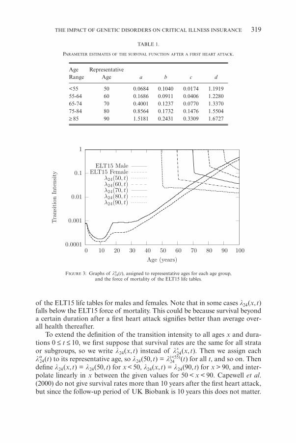
FIGURE 3: Graphs of la24(t), assigned to representative ages for each age group,
and the force of mortality of the ELT15 life tables.
of the ELT15 life tables for males and females. Note that in some cases l24(x,t)falls below the ELT15 force of mortality. This could be because survival beyonda certain duration after a first heart attack signifies better than average over-all health thereafter.
To extend the definition of the transition intensity to all ages x and dura-tions 0 ≤ t ≤ 10, we first suppose that survival rates are the same for all strataor subgroups, so we write l24(x, t) instead of ls
24(x, t). Then we assign eachla
24(t) to its representative age, so l24(50,t) = l24(<55)(t) for all t, and so on. Then
define l24(x, t) = l24(50, t) for x < 50, l24(x, t) = l24(90, t) for x > 90, and inter-polate linearly in x between the given values for 50 < x < 90. Capewell et al.(2000) do not give survival rates more than 10 years after the first heart attack,but since the follow-up period of UK Biobank is 10 years this does not matter.
THE IMPACT OF GENETIC DISORDERS ON CRITICAL ILLNESS INSURANCE 319
TABLE 1.
PARAMETER ESTIMATES OF THE SURVIVAL FUNCTION AFTER A FIRST HEART ATTACK.
Age RepresentativeRange Age a b c d
<55 50 0.0684 0.1040 0.0174 1.191955-64 60 0.1686 0.0911 0.0406 1.228065-74 70 0.4001 0.1237 0.0770 1.337075-84 80 0.8564 0.1732 0.1476 1.5504≥ 85 90 1.5181 0.2431 0.3309 1.6727
9130-06_Astin_36/2_01 06-12-2006 11:53 Pagina 319
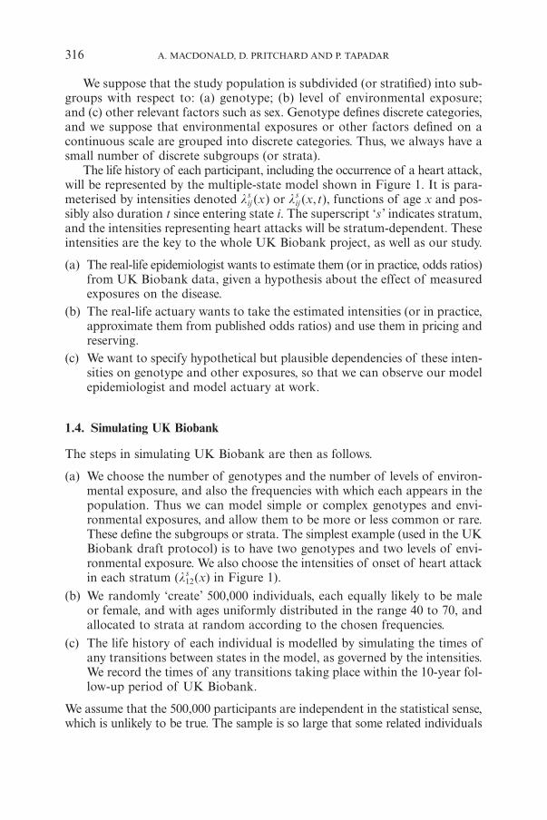
2.4. Mortality Before First Heart Attacks
The mortality intensity for persons aged x in stratum s, who do not experiencea heart attack, is given by ls
13(x). Again, we assume that this is the same in allstrata, so we just write l13(x). Let Pij(y, z) denote the conditional probabilitythat a person is in state j at age z, given that he or she was in state i at age y.Then we have:
, ,
, , , ,
P x P x
P z z P y y P y z y z y dy dzl l l
0 0
0 0zx
13 14
11 13 11 12 22 2400
+ =
+ -##
] ]
] ] ^ ^ ^ ^
g g
g g h h h h; E
(4)
, expP z y y dyl l0z
11 12 130
= - +#] ^ ^^g h hh; E (5)
, , .expP y z y z y dylz y
22 240
= - --
#^ ^h h; E (6)
Further, if we assume that the overall mortality is given by the ELT15 table(for each sex) we have:
, , .expP x P x dym0 0 1 yELTx
13 140
+ = - - #] ]g g ; E (7)
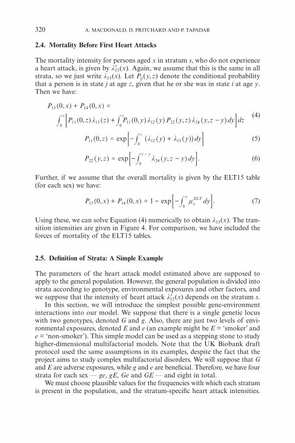
Using these, we can solve Equation (4) numerically to obtain l13(x). The tran-sition intensities are given in Figure 4. For comparison, we have included theforces of mortality of the ELT15 tables.
2.5. Definition of Strata: A Simple Example
The parameters of the heart attack model estimated above are supposed toapply to the general population. However, the general population is divided intostrata according to genotype, environmental exposures and other factors, andwe suppose that the intensity of heart attack ls
12(x) depends on the stratum s.In this section, we will introduce the simplest possible gene-environment
interactions into our model. We suppose that there is a single genetic locuswith two genotypes, denoted G and g. Also, there are just two levels of envi-ronmental exposures, denoted E and e (an example might be E = ‘smoker’ ande = ‘non-smoker’). This simple model can be used as a stepping stone to studyhigher-dimensional multifactorial models. Note that the UK Biobank draftprotocol used the same assumptions in its examples, despite the fact that theproject aims to study complex multifactorial disorders. We will suppose that Gand E are adverse exposures, while g and e are beneficial. Therefore, we have fourstrata for each sex — ge, gE, Ge and GE — and eight in total.
We must choose plausible values for the frequencies with which each stratumis present in the population, and the stratum-specific heart attack intensities.
320 A. MACDONALD, D. PRITCHARD AND P. TAPADAR
9130-06_Astin_36/2_01 06-12-2006 11:53 Pagina 320
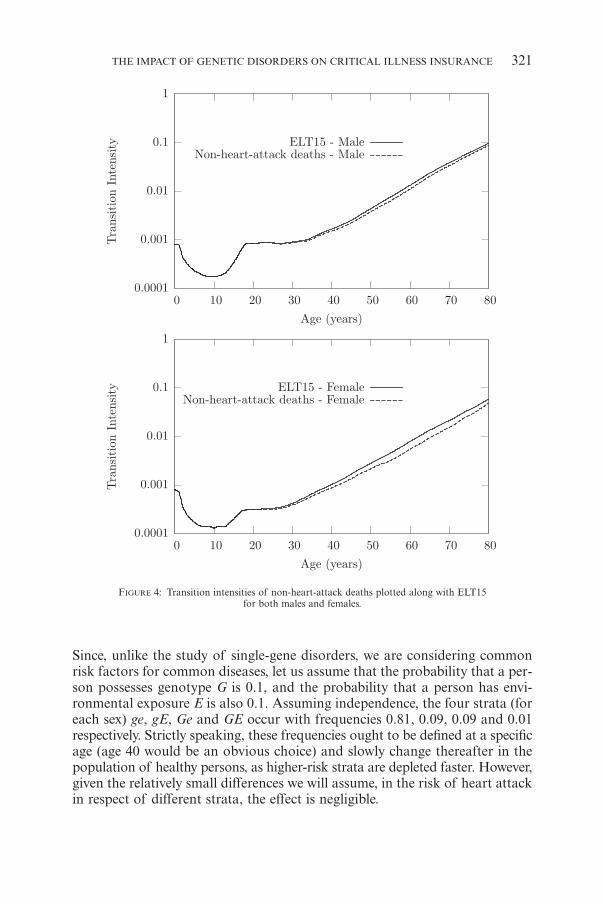
FIGURE 4: Transition intensities of non-heart-attack deaths plotted along with ELT15for both males and females.
Since, unlike the study of single-gene disorders, we are considering commonrisk factors for common diseases, let us assume that the probability that a per-son possesses genotype G is 0.1, and the probability that a person has envi-ronmental exposure E is also 0.1. Assuming independence, the four strata (foreach sex) ge, gE, Ge and GE occur with frequencies 0.81, 0.09, 0.09 and 0.01respectively. Strictly speaking, these frequencies ought to be defined at a specificage (age 40 would be an obvious choice) and slowly change thereafter in thepopulation of healthy persons, as higher-risk strata are depleted faster. However,given the relatively small differences we will assume, in the risk of heart attackin respect of different strata, the effect is negligible.
THE IMPACT OF GENETIC DISORDERS ON CRITICAL ILLNESS INSURANCE 321
9130-06_Astin_36/2_01 06-12-2006 11:53 Pagina 321
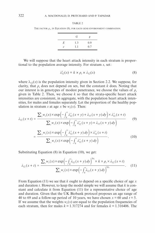
We will suppose that the heart attack intensity in each stratum is propor-tional to the population average intensity. For stratum s, set :
ls12(x) = k ≈ rs ≈ l12(x) (8)
where l12(x) is the population intensity given in Section 2.2. We suppose, forclarity, that rs does not depend on sex, but the constant k does. Noting thatour interest is in genotypes of modest penetrance, we choose the values of rs
given in Table 2. Then, we choose k so that the strata-specific heart attackintensities are consistent, in aggregate, with the population heart attack inten-sities, for males and females separately. Let the proportion of the healthy pop-ulation in stratum s at age x be ws(x). Then:
s
s
exp
expx t
w x x y x y dy
w x x y x y dy x tl
l l
l l l
st
s
st ss
12
12 130
12 130
12
#
# #
+ =- + + +
- + + + +
#
#
!
!]
] ^ ^c
] ^ ^c ]
g
g h h m
g h h m g
(9)
s
s
.exp
exp
w x x y dy
w x x y dy x t
l
l l
st
s
st ss
120
120
12
#
# #
=- +
- + +
#
#
!
!
] ^c
] ^c ]
g h m
g h m g
(10)
Substituting Equation (8) in Equation (10), we get:
s
s
.exp
expx t
w x x y dy
w x x y dy k x tl
l
l r l
t k
s
t k
ss
r
r
12
120
120
12
s
s
#
# # # #
+ =
- +
- + +
#
#
!
!]
] ^c
] ^c ]
g
g h m
g h m g
(11)
From Equation (11) we see that k ought to depend on a specific choice of age xand duration t. However, to keep the model simple we will assume that k is con-stant and calculate it from Equation (11) for a representative choice of ageand duration. Given that the UK Biobank protocol proposes an age range of40 to 69 and a follow-up period of 10 years, we have chosen x = 60 and t = 5.If we assume that the weights ws(x) are equal to the population frequencies ofeach stratum, then for males k = 1.317274 and for females k = 1.316406. The
322 A. MACDONALD, D. PRITCHARD AND P. TAPADAR
TABLE 2
THE FACTOR rs, IN EQUATION (8), FOR EACH GENE-ENVIRONMENT COMBINATION.
G g
E 1.3 0.9e 1.1 0.7
9130-06_Astin_36/2_01 06-12-2006 11:54 Pagina 322
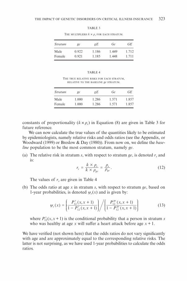
constants of proportionality (k ≈ rs) in Equation (8) are given in Table 3 forfuture reference.
We can now calculate the true values of the quantities likely to be estimatedby epidemiologists, namely relative risks and odds ratios (see the Appendix, orWoodward (1999) or Breslow & Day (1980)). From now on, we define the base-line population to be the most common stratum, namely ge.
(a) The relative risk in stratum s, with respect to stratum ge, is denoted rs andis:
s .r kk
rr
rr
ge
s
ge
s
#
#= = (12)
The values of rs are given in Table 4
(b) The odds ratio at age x in stratum s, with respect to stratum ge, based on1-year probabilities, is denoted cs(x) and is given by:
,,
,,
xP x x
P x xP x x
P x x1 1
1
1 1
1s s
s
ge
ge
12
12
12
12=- +
+
- +
+c
J
L
KK
J
L
KK]
]
]
]
]N
P
OO
N
P
OOg
g
g
g
g(13)
where P s12(x,x + 1) is the conditional probability that a person in stratum s
who was healthy at age x will suffer a heart attack before age x + 1.
We have verified (not shown here) that the odds ratios do not vary significantlywith age and are approximately equal to the corresponding relative risks. Thelatter is not surprising, as we have used 1-year probabilities to calculate the oddsratios.
THE IMPACT OF GENETIC DISORDERS ON CRITICAL ILLNESS INSURANCE 323
TABLE 3
THE MULTIPLIERS k ≈ rs FOR EACH STRATUM.
Stratum ge gE Ge GE
Male 0.922 1.186 1.449 1.712Female 0.921 1.185 1.448 1.711
TABLE 4
THE TRUE RELATIVE RISKS FOR EACH STRATUM,RELATIVE TO THE BASELINE ge STRATUM.
Stratum ge gE Ge GE
Male 1.000 1.286 1.571 1.857Female 1.000 1.286 1.571 1.857
9130-06_Astin_36/2_01 06-12-2006 11:54 Pagina 323
324 A. MACDONALD, D. PRITCHARD AND P. TAPADAR
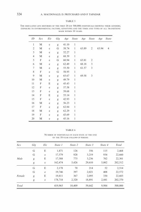
TABLE 5
THE SIMULATED LIFE HISTORIES OF THE FIRST 20 (OF 500,000) INDIVIDUALS SHOWING THEIR GENDERS,EXPOSURE TO ENVIRONMENTAL FACTORS, GENOTYPES AND THE TIMES AND TYPES OF ALL TRANSITIONS
MADE WITHIN 10 YEARS.
ID Sex E/e G/g Age State Age State Age State
1 M e g 41.10 1
2 M e G 58.74 1 63.89 2 63.94 4
3 M e g 52.27 1
4 M e g 68.39 1
5 F e G 60.94 1 63.81 2
6 M e g 62.49 1 68.18 3
7 M e g 55.50 1 61.57 3
8 F e G 58.95 1
9 M e g 65.67 1 69.58 3
10 M e g 49.79 1
11 F E g 45.43 1
12 F e g 57.58 1
13 F e g 59.68 1
14 F E g 55.14 1
15 F e g 42.93 1
16 M e g 56.23 1
17 F e g 62.84 1
18 M e g 62.29 1
19 F e g 43.69 1
20 M e g 45.16 1
TABLE 6
NUMBER OF INDIVIDUALS IN EACH STATE AT THE END
OF THE 10-YEAR FOLLOW-UP PERIOD.
Sex G/g E/e State 1 State 2 State 3 State 4 Total
G E 1,871 126 356 115 2,468
G e 17,579 928 3,219 934 22,660
Male g E 17,588 775 3,236 702 22,301
g e 162,474 5,426 29,610 5,002 202,512
G E 2,178 70 214 52 2,514
G e 19,746 397 2,021 408 22,572
Female g E 19,811 367 2,095 330 22,603
g e 178,718 2,320 18,891 2,441 202,370
Total 419,965 10,409 59,642 9,984 500,000
9130-06_Astin_36/2_01 06-12-2006 11:54 Pagina 324

3. ANALYSIS
3.1. A Sample Realisation of UK Biobank
With the parameterised model, we simulated the life histories of 500,000 peo-ple recruited to UK Biobank and followed up for 10 years. Their ages at entryare uniformly distributed between 40 and 70. This is a much simplified repre-sentation of the true UK Biobank sampling protocol (www.ukbiobank.ac.uk/docs/draft_protocol.pdf, Section 2.3). In principle sampling should be withoutreplacement from the UK population at these ages, whereas we effectively sam-ple with replacement. In practice recruitment will be via participating medicalpractices, and there may be attempts (not defined very precisely) to select theseso as to obtain a more uniform sample of different ages. Our simple assumptionshould adequately represent the UK Biobank sample; we doubt it would beworthwhile to go further in trying to reproduce it.
3.2. Epidemiological Analysis
The life histories of the first 20 people are shown in Table 5. Consider personNo. 2. He is a male with the adverse allele G, exposed to the beneficial envi-ronment e. He entered the study healthy (State 1) at age 58.74. He had a heartattack (moved to State 2) at age 63.89 and died (moved to State 4) at age 63.94.The numbers of people in each state at the end of the 10-year follow-up periodare given in Table 6.
Apart from the 500,000 life histories, the following information is availableto the epidemiologist to carry out a matched case-control study:
(a) the framework of the UK Biobank project;(b) the structure of the 4-state heart attack model given in Section 2.1;(c) the transition intensities given in Sections 2.2 to 2.4;(d) the stratum to which each person is allocated; and(e) the proportion ws(x) of individuals in each stratum at a particular age x,
say 60.
The first step is to define the cases and controls. Here, clearly, the cases are per-sons who had first heart attacks during the study period.
In real studies, epidemiologists will face problems such as missing data andcost constraints, and in most circumstances they will use only a subset of allcases for their analysis. Here, we have no such problems, unless we choose tomodel them. So, in the first instance, we will include all cases in the analysis.Later, we will consider the more realistic possibility that a subset of all casesis used.
An appropriate matching strategy is particularly important for a matchedcase-control study. Firstly, we match controls with cases by age. Suppose, forexample, that we are comparing stratum s with the baseline stratum ge, and that
THE IMPACT OF GENETIC DISORDERS ON CRITICAL ILLNESS INSURANCE 325
9130-06_Astin_36/2_01 06-12-2006 11:54 Pagina 325
a case entered the study at age x last birthday and had a heart attack at agex + t last birthday. A matched control is a person chosen randomly from per-sons in these two strata who also entered the study at age x last birthday andremained healthy at least until age x + t + 1 last birthday. Once chosen as acontrol, that person cannot be chosen as a control again. As controls are plen-tiful compared with cases, we will match 5 controls to each case, called a 1:5matching strategy. In Section 1.2, we mentioned that the genotyping of indi-viduals will be done as and when it is required. So, it might be necessary togenotype a large number of people to ensure that enough controls are availablefor a 1:5 case-control study. Other matching strategies with fewer controls percase will obviously be cheaper to implement.
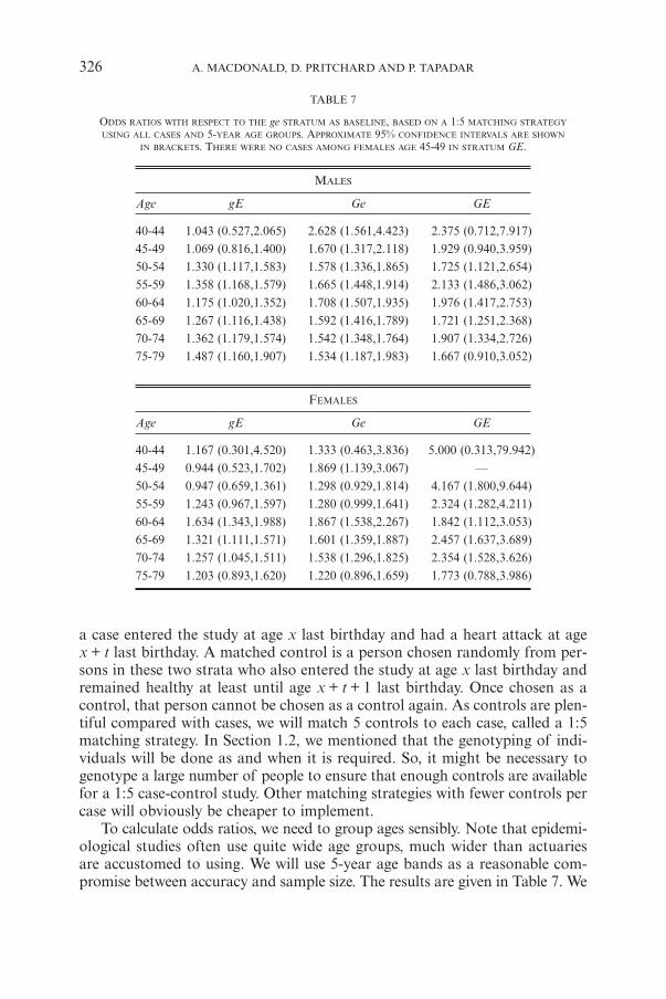
To calculate odds ratios, we need to group ages sensibly. Note that epidemi-ological studies often use quite wide age groups, much wider than actuariesare accustomed to using. We will use 5-year age bands as a reasonable com-promise between accuracy and sample size. The results are given in Table 7. We
326 A. MACDONALD, D. PRITCHARD AND P. TAPADAR
TABLE 7
ODDS RATIOS WITH RESPECT TO THE ge STRATUM AS BASELINE, BASED ON A 1:5 MATCHING STRATEGY
USING ALL CASES AND 5-YEAR AGE GROUPS. APPROXIMATE 95% CONFIDENCE INTERVALS ARE SHOWN
IN BRACKETS. THERE WERE NO CASES AMONG FEMALES AGE 45-49 IN STRATUM GE.
MALES
Age gE Ge GE
40-44 1.043 (0.527,2.065) 2.628 (1.561,4.423) 2.375 (0.712,7.917)45-49 1.069 (0.816,1.400) 1.670 (1.317,2.118) 1.929 (0.940,3.959)50-54 1.330 (1.117,1.583) 1.578 (1.336,1.865) 1.725 (1.121,2.654)55-59 1.358 (1.168,1.579) 1.665 (1.448,1.914) 2.133 (1.486,3.062)60-64 1.175 (1.020,1.352) 1.708 (1.507,1.935) 1.976 (1.417,2.753)65-69 1.267 (1.116,1.438) 1.592 (1.416,1.789) 1.721 (1.251,2.368)70-74 1.362 (1.179,1.574) 1.542 (1.348,1.764) 1.907 (1.334,2.726)75-79 1.487 (1.160,1.907) 1.534 (1.187,1.983) 1.667 (0.910,3.052)
FEMALES
Age gE Ge GE
40-44 1.167 (0.301,4.520) 1.333 (0.463,3.836) 5.000 (0.313,79.942)45-49 0.944 (0.523,1.702) 1.869 (1.139,3.067) —50-54 0.947 (0.659,1.361) 1.298 (0.929,1.814) 4.167 (1.800,9.644)55-59 1.243 (0.967,1.597) 1.280 (0.999,1.641) 2.324 (1.282,4.211)60-64 1.634 (1.343,1.988) 1.867 (1.538,2.267) 1.842 (1.112,3.053)65-69 1.321 (1.111,1.571) 1.601 (1.359,1.887) 2.457 (1.637,3.689)70-74 1.257 (1.045,1.511) 1.538 (1.296,1.825) 2.354 (1.528,3.626)75-79 1.203 (0.893,1.620) 1.220 (0.896,1.659) 1.773 (0.788,3.986)
9130-06_Astin_36/2_01 06-12-2006 11:54 Pagina 326
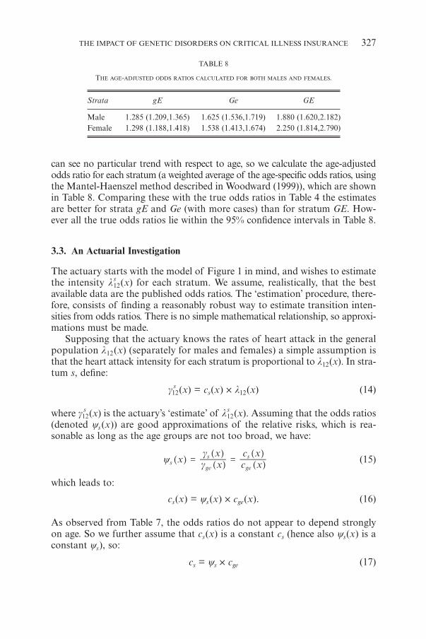
can see no particular trend with respect to age, so we calculate the age-adjustedodds ratio for each stratum (a weighted average of the age-specific odds ratios, usingthe Mantel-Haenszel method described in Woodward (1999)), which are shownin Table 8. Comparing these with the true odds ratios in Table 4 the estimatesare better for strata gE and Ge (with more cases) than for stratum GE. How-ever all the true odds ratios lie within the 95% confidence intervals in Table 8.
3.3. An Actuarial Investigation
The actuary starts with the model of Figure 1 in mind, and wishes to estimatethe intensity ls
12(x) for each stratum. We assume, realistically, that the bestavailable data are the published odds ratios. The ‘estimation’ procedure, there-fore, consists of finding a reasonably robust way to estimate transition inten-sities from odds ratios. There is no simple mathematical relationship, so approxi-mations must be made.
Supposing that the actuary knows the rates of heart attack in the generalpopulation l12(x) (separately for males and females) a simple assumption isthat the heart attack intensity for each stratum is proportional to l12(x). In stra-tum s, define:
g s12(x) = cs(x) ≈ l12(x) (14)
where g s12(x) is the actuary’s ‘estimate’ of ls
12(x). Assuming that the odds ratios(denoted cs(x)) are good approximations of the relative risks, which is rea-sonable as long as the age groups are not too broad, we have:
x xx
xx
sge
s
ge
s= = cc
gg
c ]]
]
]
]g
g
g
g
g (15)
which leads to:
cs(x) = cs(x) ≈ cge(x). (16)
As observed from Table 7, the odds ratios do not appear to depend stronglyon age. So we further assume that cs(x) is a constant cs (hence also cs(x) is aconstant cs), so:
cs = cs ≈ cge (17)
THE IMPACT OF GENETIC DISORDERS ON CRITICAL ILLNESS INSURANCE 327
TABLE 8
THE AGE-ADJUSTED ODDS RATIOS CALCULATED FOR BOTH MALES AND FEMALES.
Strata gE Ge GE
Male 1.285 (1.209,1.365) 1.625 (1.536,1.719) 1.880 (1.620,2.182)Female 1.298 (1.188,1.418) 1.538 (1.413,1.674) 2.250 (1.814,2.790)
9130-06_Astin_36/2_01 06-12-2006 11:54 Pagina 327

where cs is the age-adjusted odds ratio. Thus Equation (14) becomes:
g s12(x) = cge ≈ cs ≈ l12(x). (18)
Now Equation (11) can be written:
s
s
s
s s
.exp
expx t
w x x y dy
w x x y dy x tl
l
l l
ge
t
s
ge
t
ges
12
120
120
12
+ =- +
- + +
c
c c
c
c c
#
#
!
!]
] ^c
] ^c ]
g
g h m
g h m g
(19)
Let us assume that at age x = 60, the ws(x) are given by the population fre-quencies of the respective strata. Now we can solve Equation (19) for the mul-tiplier cge for a particular choice of age x and any duration t. Then we can useEquation (17) to obtain cs for s = gE, Ge and GE. We find (not shown here)that the results are very similar for different values of t. In Table 9, we showthe ‘estimated’ cs for representative age x = 60 and duration t = 5, based on theage-adjusted odds ratios in Table 8. These values can be compared with the truevalues given in Table 3. They are in good agreement for strata s = ge, gE andGe. The agreement for stratum s = GE is not so good, but it was based on asmall number of cases, 241 males and 122 females.
3.4. Premium Rating for Critical Illness Insurance
The actuary will use the intensities g s12(x) ‘estimated’ in Section 3.3 to calcu-
late CI insurance premiums. We use the CI insurance model from Gutiérrez &Macdonald (2003), assuming that all intensities except those for heart attackare as given there. For heart attack, we use the intensities g s
12(x). We computeexpected present values by solving Thiele’s differential equations numerically,with a force of interest of d = 0.044017 (see Norberg (1995)).
Table 10 shows the true premiums for the strata s = ge, Ge and GE, as a per-centage of the premiums for stratum ge, for males and females and for differentages and terms. Here, ‘true’ means that they have been computed using theintensities ls
12(x), not the actuary’s estimates. Table 11 then shows the corre-sponding premiums, as a percentage of those charged for stratum ge, using
328 A. MACDONALD, D. PRITCHARD AND P. TAPADAR
TABLE 9
THE ESTIMATED MULTIPLIERS cs FOR EACH STRATUM.
Stratum ge gE Ge GE
Male 0.918 1.179 1.492 1.726Female 0.920 1.194 1.415 2.070
9130-06_Astin_36/2_01 06-12-2006 11:55 Pagina 328

THE IMPACT OF GENETIC DISORDERS ON CRITICAL ILLNESS INSURANCE 329
TABLE 10
THE TRUE CRITICAL ILLNESS INSURANCE PREMIUMS FOR DIFFERENT STRATA
AS A PERCENTAGE OF THOSE FOR STRATUM ge.
Stratum Males Females
Term Term
Age 5 15 25 35 Age 5 15 25 35
45 112% 111% 109% 107% 45 103% 103% 104% 104%
gE55 110% 108% 107% 55 104% 105% 105%65 107% 106% 65 105% 106%75 106% 75 106%
45 124% 121% 117% 115% 45 105% 107% 108% 108%
Ge55 119% 116% 114% 55 109% 110% 110%65 114% 112% 65 111% 111%75 111% 75 111%
45 136% 131% 126% 122% 45 108% 110% 112% 112%
GE55 129% 124% 121% 55 113% 115% 115%65 120% 118% 65 116% 117%75 117% 75 117%
TABLE 11
THE ACTUARY’S ESTIMATED CRITICAL ILLNESS INSURANCE PREMIUMS FOR DIFFERENT STRATA
AS A PERCENTAGE OF THOSE FOR STRATUM ge.
Stratum Males Females
Term Term
Age 5 15 25 35 Age 5 15 25 35
45 112% 110% 109% 107% 45 103% 104% 104% 104%
gE55 110% 108% 107% 55 105% 105% 105%65 107% 106% 65 106% 106%75 106% 75 106%
45 126% 123% 119% 116% 45 105% 106% 108% 108%
Ge55 121% 117% 115% 55 108% 109% 109%65 115% 113% 65 110% 110%75 112% 75 111%
45 137% 132% 126% 123% 45 111% 115% 118% 118%
GE55 129% 124% 121% 55 119% 121% 121%65 121% 119% 65 124% 124%75 117% 75 125%
9130-06_Astin_36/2_01 06-12-2006 11:55 Pagina 329
the actuary’s estimates g s12(x). The results are similar to those in Table 10. The
estimates are good for strata gE and Ge, but not as accurate for females in stra-tum GE. As mentioned before, this stratum had relatively few cases.
4. SIMULATION RESULTS
4.1. Varying the Genetic and Environment Model
In the last section, we estimated parameters of a heart attack model and theresulting CI insurance premiums, based on a simulated realisation of UK Bio-bank. The underlying ‘true’ model (chosen by us) was particularly simple — twogenotypes, two environmental exposures and proportional hazards of heartattack — and by great good luck, our model epidemiologist hit upon exactlythe correct hypotheses in fitting his/her model. So it is not surprising thathe/she obtained good parameter estimates, with the possible exception of thosein respect of the smallest stratum, GE.
In reality, the epidemiologist faces more difficult problems:
(a) There is likely to be more than one gene, many with more than two variants,as candidates for influencing the disease.
(b) Similarly, there are likely to be several environmental exposures of interest.(c) Model mis-specification is always possible (indeed, it may be the norm).(d) On grounds of cost, the number of cases and the number of controls per case
may be limited.(e) As mentioned earlier, UK Biobank will be a single unrepeatable sample, hence
sampling error will be present. Although 500,000 seems like a huge sample,it may not be when smaller numbers of cases are sampled from within it.
In a simulation study, we are in a position to explore these problems. In par-ticular, we can address (d) and (e) above, because we can replicate the entireUK Biobank dataset many times, and repeat the epidemiological and actuarialanalyses using each realisation. Thus we can estimate the sampling distributionsof parameter estimates and premium rates, while the analysis of the singlerealization in Section 3 only gave us point estimates of the latter. (We did giveapproximate confidence intervals of the estimated odds ratios, because theycan be derived on theoretical grounds. This is not possible for such a complicatedfunction of the model parameters as a premium rate, and simulation is one ofthe few practical approaches.) We concentrate on this question in the rest ofthis paper, because it is directly relevant to the approach adopted by GAIC inthe UK, and likely to be adopted by similar bodies elsewhere, which demandsthat the reliability of prognoses based on genetic information must be demon-strated if they are to be used in any way. In the case of multifactorial disorders,we assume that this requirement is to be interpreted in the statistical sense ratherthan as applying to individual applicants. Our exploration of (a), (b) and (c)above will be the subject of a future paper.
330 A. MACDONALD, D. PRITCHARD AND P. TAPADAR
9130-06_Astin_36/2_01 06-12-2006 11:55 Pagina 330

In addition to simulating many replications of UK Biobank, we willconsider the effect of stronger or weaker genetic and environmental effects,and of more common and less common adverse genotypes. We call each suchvariant of the underlying model a ‘scenario’, which should not be confused withthe simulation procedure discussed above. We will hold each scenario fixed, andthen simulate outcomes of UK Biobank under those assumptions.
We have already introduced one set of assumptions in Section 2, which wewill refer to as our Base scenario. The details of all the scenarios are given inTable 12. The parameters that must be specified are:
(a) The population frequency of each stratum (the same for males and females).(b) The parameters k for each sex and rs for each stratum. Although rs does
not depend on sex, for convenience Table 12 shows the combined con-stants of proportionality k ≈ rs for each sex.
THE IMPACT OF GENETIC DISORDERS ON CRITICAL ILLNESS INSURANCE 331
TABLE 12
THE MODEL PARAMETERS FOR DIFFERENT SCENARIOS. ODDS RATIOS ARE ALSO SHOWN.
Penetrance FrequencyParameters Stratum Base
Low High Low High
ge 0.81 0.81 0.81 0.9025 0.64Population gE 0.09 0.09 0.09 0.0475 0.16Frequency Ge 0.09 0.09 0.09 0.0475 0.16
GE 0.01 0.01 0.01 0.0025 0.04
ge 0.70 0.85 0.55 0.70 0.70
rsgE 0.90 0.95 0.85 0.90 0.90Ge 1.10 1.05 1.15 1.10 1.10GE 1.30 1.15 1.45 1.30 1.30
k (Male) All 1.317274 1.136603 1.568090 1.370745 1.221620k (Female) All 1.316406 1.136463 1.564821 1.370230 1.220385
ge 0.922 0.966 0.862 0.960 0.855k ≈ rs gE 1.186 1.080 1.333 1.234 1.099(Male) Ge 1.449 1.193 1.803 1.508 1.344
GE 1.712 1.307 2.274 1.782 1.588
ge 0.921 0.966 0.861 0.959 0.854k ≈ rs gE 1.185 1.080 1.330 1.233 1.098(Female) Ge 1.448 1.193 1.800 1.507 1.342
GE 1.711 1.307 2.269 1.781 1.587
ge 1.000 1.000 1.000 1.000 1.000gE 1.286 1.118 1.545 1.286 1.286
Odds RatioGe 1.571 1.235 2.091 1.571 1.571GE 1.857 1.353 2.636 1.857 1.857
9130-06_Astin_36/2_01 06-12-2006 11:55 Pagina 331
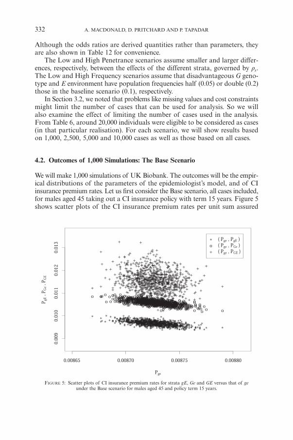
FIGURE 5: Scatter plots of CI insurance premium rates for strata gE, Ge and GE versus that of geunder the Base scenario for males aged 45 and policy term 15 years.
Although the odds ratios are derived quantities rather than parameters, theyare also shown in Table 12 for convenience.
The Low and High Penetrance scenarios assume smaller and larger differ-ences, respectively, between the effects of the different strata, governed by rs.The Low and High Frequency scenarios assume that disadvantageous G geno-type and E environment have population frequencies half (0.05) or double (0.2)those in the baseline scenario (0.1), respectively.
In Section 3.2, we noted that problems like missing values and cost constraintsmight limit the number of cases that can be used for analysis. So we willalso examine the effect of limiting the number of cases used in the analysis.From Table 6, around 20,000 individuals were eligible to be considered as cases(in that particular realisation). For each scenario, we will show results basedon 1,000, 2,500, 5,000 and 10,000 cases as well as those based on all cases.
4.2. Outcomes of 1,000 Simulations: The Base Scenario
We will make 1,000 simulations of UK Biobank. The outcomes will be the empir-ical distributions of the parameters of the epidemiologist’s model, and of CIinsurance premium rates. Let us first consider the Base scenario, all cases included,for males aged 45 taking out a CI insurance policy with term 15 years. Figure 5shows scatter plots of the CI insurance premium rates per unit sum assured
332 A. MACDONALD, D. PRITCHARD AND P. TAPADAR
9130-06_Astin_36/2_01 06-12-2006 11:55 Pagina 332
for strata gE, Ge and GE versus those of ge. More precisely, the outcome ofthe i th simulation is a drawing pi = (pi
ge, pigE, pi
Ge, piGE) from the sampling distri-
bution of the 4-dimensional random variable P = (Pge, PgE, PGe, PGE), where Ps
is the premium rate in stratum s.The scatter plots show clearly that the premium rate pairs (Pge,PgE ) and
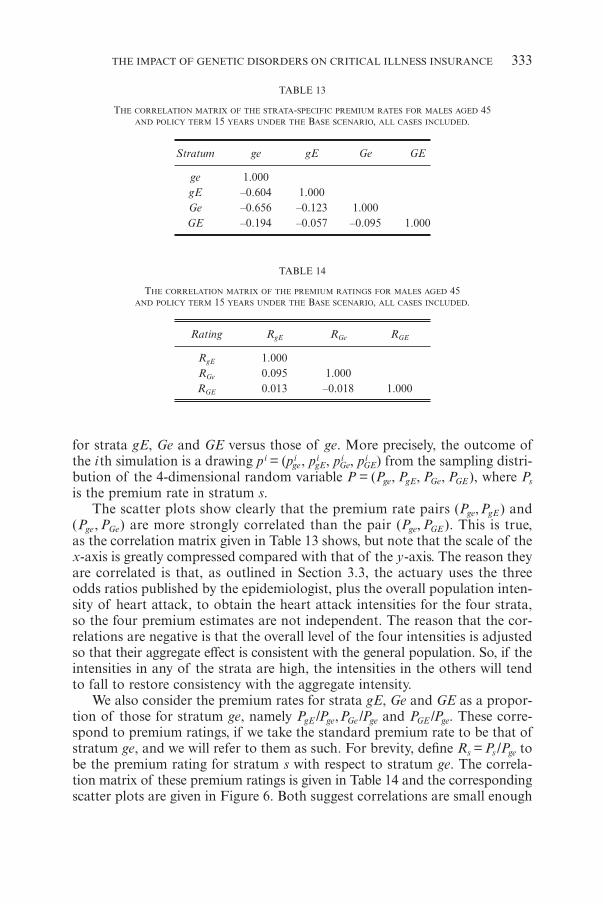
(Pge, PGe) are more strongly correlated than the pair (Pge, PGE ). This is true,as the correlation matrix given in Table 13 shows, but note that the scale of thex-axis is greatly compressed compared with that of the y-axis. The reason theyare correlated is that, as outlined in Section 3.3, the actuary uses the threeodds ratios published by the epidemiologist, plus the overall population inten-sity of heart attack, to obtain the heart attack intensities for the four strata,so the four premium estimates are not independent. The reason that the cor-relations are negative is that the overall level of the four intensities is adjustedso that their aggregate effect is consistent with the general population. So, if theintensities in any of the strata are high, the intensities in the others will tendto fall to restore consistency with the aggregate intensity.
We also consider the premium rates for strata gE, Ge and GE as a propor-tion of those for stratum ge, namely PgE/Pge,PGe/Pge and PGE/Pge. These corre-spond to premium ratings, if we take the standard premium rate to be that ofstratum ge, and we will refer to them as such. For brevity, define Rs = Ps/Pge tobe the premium rating for stratum s with respect to stratum ge. The correla-tion matrix of these premium ratings is given in Table 14 and the correspondingscatter plots are given in Figure 6. Both suggest correlations are small enough
THE IMPACT OF GENETIC DISORDERS ON CRITICAL ILLNESS INSURANCE 333
TABLE 13
THE CORRELATION MATRIX OF THE STRATA-SPECIFIC PREMIUM RATES FOR MALES AGED 45AND POLICY TERM 15 YEARS UNDER THE BASE SCENARIO, ALL CASES INCLUDED.
Stratum ge gE Ge GE
ge 1.000gE –0.604 1.000Ge –0.656 –0.123 1.000GE –0.194 –0.057 –0.095 1.000
TABLE 14
THE CORRELATION MATRIX OF THE PREMIUM RATINGS FOR MALES AGED 45AND POLICY TERM 15 YEARS UNDER THE BASE SCENARIO, ALL CASES INCLUDED.
Rating RgE RGe RGE
RgE 1.000RGe 0.095 1.000RGE 0.013 –0.018 1.000
9130-06_Astin_36/2_01 06-12-2006 11:55 Pagina 333
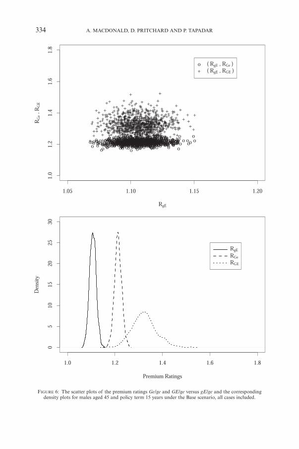
FIGURE 6: The scatter plots of the premium ratings Ge/ge and GE/ge versus gE/ge and the correspondingdensity plots for males aged 45 and policy term 15 years under the Base scenario, all cases included.
334 A. MACDONALD, D. PRITCHARD AND P. TAPADAR
9130-06_Astin_36/2_01 06-12-2006 11:55 Pagina 334

to neglect, which means that instead of always considering the full joint dis-tribution of the premiums P, we can obtain all the information of interest byseparate examination of the marginal distributions of the premium ratings.The densities of these marginal distributions are given in Figure 6. This imme-diately suggests a simple approach to the questions that GAIC must ask, becausethe reliability of the premium rating in each stratum — in terms of its distin-guishability from the premium ratings in the other strata — is revealed by thedegree to which its marginal density overlaps the marginal densities of the others.Presented with Figure 6, we might expect GAIC to agree that strata Ge andGE had premium ratings distinct from that of stratum gE, but to ask whetheror not they had premium ratings reliably distinct from each other.
4.3. A Measure of Confidence
Our precise formulation of the question that GAIC might now ask is: arethe marginal empirical distributions of premium ratings in different stratasufficiently different to support charging different premiums (when doing sois allowed)? In this section, we suggest a simple measure to address this.
Let X and Y be two continuous random variables with cumulative distribu-tion functions FX and FY respectively. We can find u such that FX(u) + FY(u) = 1.If the ranges of X and Y overlap, u lies in both and is unique, otherwise anyu that lies between their ranges will do. This can be rewritten as FX(u) = 1 – FY(u),or P[X ≤ u ] = P[Y > u ].
Without loss of generality, let us also assume that FX(u) ≥ FY(u). Defineour measure of confidence to be 2 ≈ FX (u) – 1, which gives a measure of theoverlap of FX and FY. Denote this O (X,Y ), or just O if the context is clear. IfFX(u) = FY(u) = 0.5, then we are as unsure as we can be that FX and FY are dis-tinct, and O = 0. As FX(u) increases to 1, the area of overlap decreases. If theranges of X and Y do not overlap at all, FX(u) = 1 and we have high confidencein deciding that FX and FY are distinct; in this case O = 1.
4.4. Results
In this section, we simulate 1,000 realisations of UK Biobank under each sce-nario outlined in Table 12. Our aim is to examine how reliably UK Biobankmight identify differences in premium ratings, as a body like GAIC mightrequire. This is measured by the three quantities O (RgE,RGe), O (RGe,RGE) andO (RgE,RGE). We have verified (not shown here) that these do not vary significantlyby age or policy term, so in Table 15, we present results for a representativepolicy for males aged 45 and policy term 15 years.
Note that it is impossible to calculate an odds ratio for a given age groupunless there is at least one case in that age group in each stratum. A few of the1,000 simulations failed this criterion, and these were omitted from the resultsin Table 15. Those affected were the Base and the Low Penetrance scenarios
THE IMPACT OF GENETIC DISORDERS ON CRITICAL ILLNESS INSURANCE 335
9130-06_Astin_36/2_01 06-12-2006 11:55 Pagina 335
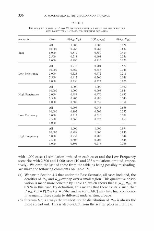
with 1,000 cases (1 simulation omitted in each case) and the Low Frequencyscenarios with 2,500 and 1,000 cases (10 and 238 simulations omitted, respec-tively). We omit the last of these from the table as being possibly misleading.We make the following comments on Table 15:
(a) We saw in Section 4.3 that under the Base Scenario, all cases included, thedensities of RGe and RGE overlap over a small region. This qualitative obser-vation is made more concrete by Table 15, which shows that O (RGe,RGE) =0.924 in this case. By definition, this means that there exists x such thatP[RGe< x] = P[RGE > x] = 0.962, and we (or GAIC) may have high confidencein assigning these strata to different underwriting groups.
(b) Stratum GE is always the smallest, so the distribution of RGE is always themost spread out. This is also evident from the scatter plots in Figure 6.
336 A. MACDONALD, D. PRITCHARD AND P. TAPADAR
TABLE 15
THE MEASURE OF OVERLAP O FOR CI INSURANCE PREMIUM RATINGS FOR MALES AGED 45,WITH POLICY TERM 15 YEARS, FOR DIFFERENT SCENARIOS.
Scenario Cases O (RgE,RGe) O (RgE,RGE) O (RGe,RGE)
All 1.000 1.000 0.92410,000 0.968 0.962 0.632
Base 5,000 0.872 0.850 0.4842,500 0.718 0.698 0.3561,000 0.490 0.416 0.176
All 0.918 0.904 0.57210,000 0.662 0.658 0.346
Low Penetrance 5,000 0.528 0.472 0.2162,500 0.412 0.360 0.1481,000 0.250 0.222 0.076
All 1.000 1.000 0.99210,000 1.000 0.998 0.844
High Penetrance 5,000 0.984 0.970 0.6922,500 0.906 0.886 0.5401,000 0.688 0.658 0.354
All 0.996 0.948 0.65810,000 0.892 0.706 0.352
Low Frequency 5,000 0.712 0.516 0.2082,500 0.566 0.322 0.0601,000 — — —
All 1.000 1.000 0.99410,000 0.988 1.000 0.896
High Frequency 5,000 0.932 0.986 0.7442,500 0.806 0.902 0.5461,000 0.594 0.716 0.358
9130-06_Astin_36/2_01 06-12-2006 11:55 Pagina 336
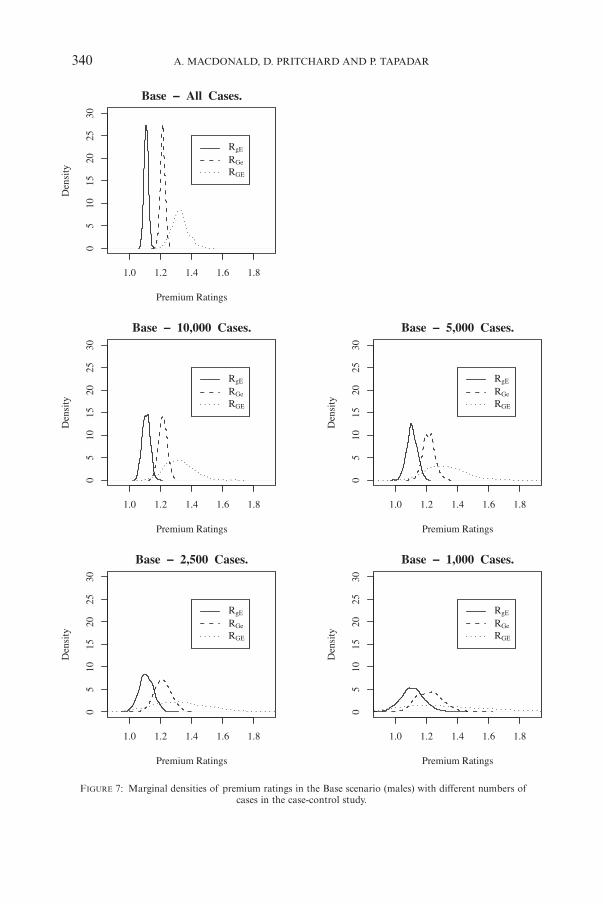
(c) We expect real case-control studies to use only a subset of cases, and Table 15shows that the effect of this is very great. For example, in the Base scenario,O (RGe,RGE) falls from 0.924 to 0.176 as the number of cases used fallsfrom ‘All’ to 1,000. Figure 7 shows, for the Base scenario, the marginaldensities with different numbers of cases. The densities overlap consider-ably if the number of cases is small (and bear in mind that 1,000 cases isnot a very small investigation by normal standards).
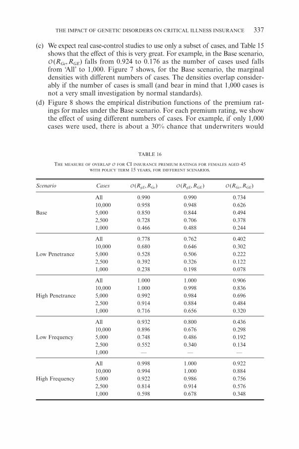
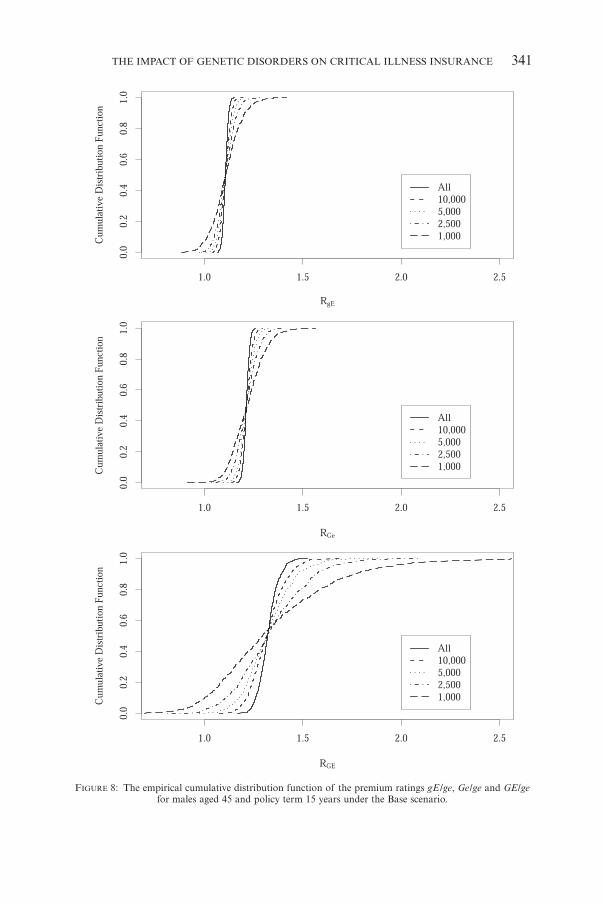
(d) Figure 8 shows the empirical distribution functions of the premium rat-ings for males under the Base scenario. For each premium rating, we showthe effect of using different numbers of cases. For example, if only 1,000cases were used, there is about a 30% chance that underwriters would
THE IMPACT OF GENETIC DISORDERS ON CRITICAL ILLNESS INSURANCE 337
TABLE 16
THE MEASURE OF OVERLAP O FOR CI INSURANCE PREMIUM RATINGS FOR FEMALES AGED 45WITH POLICY TERM 15 YEARS, FOR DIFFERENT SCENARIOS.
Scenario Cases O (RgE,RGe) O (RgE,RGE) O (RGe,RGE)
All 0.990 0.990 0.73410,000 0.958 0.948 0.626
Base 5,000 0.850 0.844 0.4942,500 0.728 0.706 0.3781,000 0.466 0.488 0.244
All 0.778 0.762 0.40210,000 0.680 0.646 0.302
Low Penetrance 5,000 0.528 0.506 0.2222,500 0.392 0.326 0.1221,000 0.238 0.198 0.078
All 1.000 1.000 0.90610,000 1.000 0.998 0.836
High Penetrance 5,000 0.992 0.984 0.6962,500 0.914 0.884 0.4841,000 0.716 0.656 0.320
All 0.932 0.800 0.43610,000 0.896 0.676 0.298
Low Frequency 5,000 0.748 0.486 0.1922,500 0.552 0.340 0.1341,000 — — —
All 0.998 1.000 0.92210,000 0.994 1.000 0.884
High Frequency 5,000 0.922 0.986 0.7562,500 0.814 0.914 0.5761,000 0.598 0.678 0.348
9130-06_Astin_36/2_01 06-12-2006 11:55 Pagina 337

338 A. MACDONALD, D. PRITCHARD AND P. TAPADAR
TABLE 17
THE MEASURE OF OVERLAP O FOR CI INSURANCE PREMIUM RATINGS FOR MALES AGED 45,WITH POLICY TERM 15 YEARS, FOR DIFFERENT SCENARIOS AND A 1:1 MATCHING STRATEGY.
Scenario Cases O (RgE,RGe) O (RgE,RGE) O (RGe,RGE)
All 0.990 0.990 0.77410,000 0.886 0.872 0.454
Base 5,000 0.740 0.720 0.3742,500 0.554 0.544 0.2481,000 0.378 0.400 0.222
All 0.808 0.820 0.45610,000 0.558 0.526 0.220
Low Penetrance 5,000 0.372 0.378 0.1882,500 0.288 0.308 0.1841,000 0.232 0.204 0.048
All 1.000 1.000 0.90810,000 0.988 0.978 0.680
High Penetrance 5,000 0.898 0.902 0.4942,500 0.762 0.742 0.3661,000 0.548 0.480 0.222
All 0.954 0.856 0.474Low Frequency 10,000 0.738 0.558 0.284
5,000 0.574 0.464 0.2282,500 — — —1,000 — — —
All 1.000 1.000 0.95010,000 0.944 0.986 0.746
High Frequency 5,000 0.826 0.932 0.5922,500 0.668 0.802 0.4561,000 0.474 0.594 0.306
TABLE 18
THE NUMBER OF SIMULATIONS REJECTED DUE TO THE INABILITY TO CALCULATE THE ODDS RATIOS
FOR A 1:1 MATCHING STRATEGY.
Number of CasesScenario
All 10,000 5,000 2,500 1,000
Base 0 0 0 0 13Low Penetrance 0 0 0 0 16High Penetrance 0 0 0 0 36Low Frequency 0 0 6 123 630High Frequency 0 0 0 0 0
9130-06_Astin_36/2_01 06-12-2006 11:55 Pagina 338
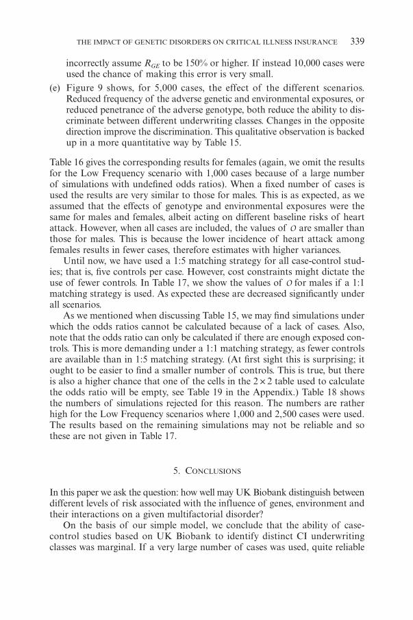
THE IMPACT OF GENETIC DISORDERS ON CRITICAL ILLNESS INSURANCE 339
incorrectly assume RGE to be 150% or higher. If instead 10,000 cases wereused the chance of making this error is very small.
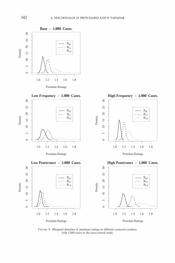
(e) Figure 9 shows, for 5,000 cases, the effect of the different scenarios.Reduced frequency of the adverse genetic and environmental exposures, orreduced penetrance of the adverse genotype, both reduce the ability to dis-criminate between different underwriting classes. Changes in the oppositedirection improve the discrimination. This qualitative observation is backedup in a more quantitative way by Table 15.
Table 16 gives the corresponding results for females (again, we omit the resultsfor the Low Frequency scenario with 1,000 cases because of a large numberof simulations with undefined odds ratios). When a fixed number of cases isused the results are very similar to those for males. This is as expected, as weassumed that the effects of genotype and environmental exposures were thesame for males and females, albeit acting on different baseline risks of heartattack. However, when all cases are included, the values of O are smaller thanthose for males. This is because the lower incidence of heart attack amongfemales results in fewer cases, therefore estimates with higher variances.
Until now, we have used a 1:5 matching strategy for all case-control stud-ies; that is, five controls per case. However, cost constraints might dictate theuse of fewer controls. In Table 17, we show the values of O for males if a 1:1matching strategy is used. As expected these are decreased significantly underall scenarios.
As we mentioned when discussing Table 15, we may find simulations underwhich the odds ratios cannot be calculated because of a lack of cases. Also,note that the odds ratio can only be calculated if there are enough exposed con-trols. This is more demanding under a 1:1 matching strategy, as fewer controlsare available than in 1:5 matching strategy. (At first sight this is surprising; itought to be easier to find a smaller number of controls. This is true, but thereis also a higher chance that one of the cells in the 2 ≈ 2 table used to calculatethe odds ratio will be empty, see Table 19 in the Appendix.) Table 18 showsthe numbers of simulations rejected for this reason. The numbers are ratherhigh for the Low Frequency scenarios where 1,000 and 2,500 cases were used.The results based on the remaining simulations may not be reliable and sothese are not given in Table 17.
5. CONCLUSIONS
In this paper we ask the question: how well may UK Biobank distinguish betweendifferent levels of risk associated with the influence of genes, environment andtheir interactions on a given multifactorial disorder?
On the basis of our simple model, we conclude that the ability of case-control studies based on UK Biobank to identify distinct CI underwritingclasses was marginal. If a very large number of cases was used, quite reliable
9130-06_Astin_36/2_01 06-12-2006 11:55 Pagina 339
340 A. MACDONALD, D. PRITCHARD AND P. TAPADAR
FIGURE 7: Marginal densities of premium ratings in the Base scenario (males) with different numbers ofcases in the case-control study.
9130-06_Astin_36/2_01 06-12-2006 11:55 Pagina 340
THE IMPACT OF GENETIC DISORDERS ON CRITICAL ILLNESS INSURANCE 341
FIGURE 8: The empirical cumulative distribution function of the premium ratings gE /ge, Ge/ge and GE/gefor males aged 45 and policy term 15 years under the Base scenario.
9130-06_Astin_36/2_01 06-12-2006 11:55 Pagina 341
342 A. MACDONALD, D. PRITCHARD AND P. TAPADAR
FIGURE 9: Marginal densities of premium ratings in different scenarios (males),with 5,000 cases in the case-control study.
9130-06_Astin_36/2_01 06-12-2006 11:55 Pagina 342
discrimination was achieved, but this is a very expensive option. If a morerealistic number of cases was used — a few thousands — the power to dis-criminate quickly diminished. In particular, it was clear that if the effects ofthe adverse genotype and adverse environment were any less than we hadassumed, the power to discriminate would be rather poor.
This conclusion ought to bring comfort to those who are worried aboutinsurers’ use of genetic information, and to insurers themselves. This is par-ticularly important during the 5 to 10 years that must pass before UK Biobankitself starts to yield results. We have found no support for the idea that verylarge-scale genetic studies like UK Biobank will lead to significant changes inunderwriting practice.
Our study has been very simple and idealised in several respects mentionedabove. Most obviously, our genetic model is not truly multifactorial, althoughit does allow for a basic environmental interaction. Further research is in handto extend the model to a more realistic, though still hypothetical, representationof a multifactorial genetic contribution to heart attack. Our aim will be to findout whether this will strengthen or weaken the discriminatory power of genetictests, along the lines that GAIC has pioneered for single-gene disorders. Anotherpoint that will repay further study is the possibility of model mis-specification.
ACKNOWLEDGEMENTS
This work was carried out at the Genetics and Insurance Research Centre atHeriot-Watt University. We would like to thank the sponsors for funding, andmembers of the Steering Committee for helpful comments at various stages.
REFERENCES
BRESLOW, N.E. and DAY, N.E. (1980) Statistical Methods in Cancer Research: Volume 1 – Theanalysis of case-control studies. International Agency for Research on Cancer.
CAPEWELL, S., LIVINGSTON, B.M., MACINTYRE, K., CHALMERS, J.W.T., BOYD, J., FINLAYSON, A.,REDPATH, A., PELL, J.P., EVANS, C.J. and MCMURRAY, J.J.V. (2000) Trends in case-fatality in117,718 patients admitted with acute myocardial infarction in Scotland. European HeartJournal, 21, 1833-1840.
DAYKIN, C.D., AKERS, D.A., MACDONALD, A.S., MCGLEENAN, T., PAUL, D. and TURVEY, P.J.(2003) Genetics and insurance – some social policy issues (with discussions). British Actu-arial Journal, 9, 787-874.
GUTIÉRREZ, C. and MACDONALD, A.S. (2003) Adult polycystic kidney disease and critical illnessinsurance. North American Actuarial Journal, 7(2), 93-115.
MACDONALD, A.S. (2004) Genetics and insurance management, in The Swedish Society of Actu-aries: One Hundred Years, ed. A. Sandström, Svenska Aktuarieföreningen, Stockholm.
MACDONALD, A.S. and PRITCHARD, D.J. (2000) A mathematical model of Alzheimer’s diseaseand the ApoE gene. ASTIN Bulletin, 30, 69-110.
NORBERG, R. (1995) Differential equations for moments of present values in life insurance. Insur-ance: Mathematics and Economics, 17, 171-180.
WOODWARD, M. (1999) Epidemiology: Study Design and Data Analysis. Chapman & Hall.
THE IMPACT OF GENETIC DISORDERS ON CRITICAL ILLNESS INSURANCE 343
9130-06_Astin_36/2_01 06-12-2006 11:55 Pagina 343
APPENDIX
A BRIEF INTRODUCTION TO CASE-CONTROL STUDIES
This appendix describes the main features of a case-control study, one of themain tools in epidemiology, but which is not well-known to actuaries. Standardreferences for this material are Woodward (1999) and Breslow & Day (1980).The question asked is: how do genetic and environmental risk factors interactto affect the risk of a disease or other outcome?
We usually want answers that are valid for the general population. The bestway to proceed is to carry out a prospective cohort study — recruit a properlyrandomised sample of healthy people, observe them over time, and see howthe suspected risk factors correlate with cases of the disease. Such a studyshould be free of any selection biases. However, it will be time consuming and(especially for rare diseases) prohibitively expensive. It is much quicker andcheaper to select a sample of people who already have the disease of interest,and a sample of people who do not have the disease, and see if the suspectedrisk factor turns up more often in the diseased sample. This is a case-controlstudy; the two samples are known as cases and controls, respectively. But,because the cases are chosen retrospectively from known sufferers of the dis-ease, the sampling may be biased. The statistical question, therefore, is whatinferences can be drawn about the general population, from a case-control studywhose cases have been selected retrospectively?
Controls should be a representative sample of disease-free individuals, whohad exactly the same chances as the cases of become diseased, except in respectof the risk factors of interest. For example, suppose we are studying the effectof smoking on lung cancer. If all the cases are over 60 years old, and all thecontrols are under 30 years old, we can hardly compare their respective risksof lung cancer. Therefore we would match controls to cases: given as a case aman age 65 who had had lung cancer, a suitable control might be a man age 65who had not. The general approach would be to match in respect of as manyfactors as possible that might affect the risk of lung cancer, except smokinghabits. Then the proportions of smokers among cases and controls ought tobe informative.
Matching reduces confounding when comparing cases and controls, butnot within each of the two groups. For example, if age is thought to affect therisk of lung cancer, we would not want to analyse as a single unit a sample of
344 A. MACDONALD, D. PRITCHARD AND P. TAPADAR
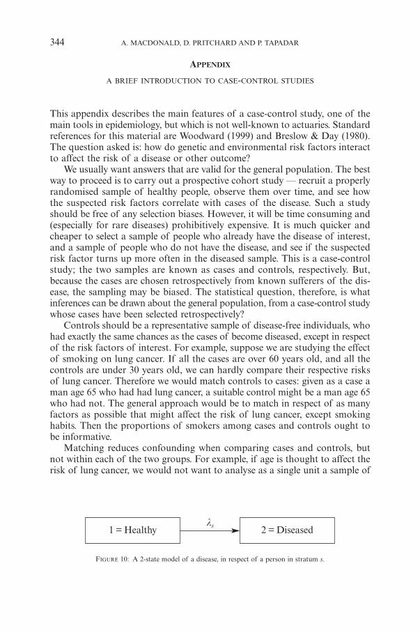
FIGURE 10: A 2-state model of a disease, in respect of a person in stratum s.
1 = Healthy 2 = Diseasedls
9130-06_Astin_36/2_01 06-12-2006 11:55 Pagina 344
cases whose ages ranged from 20 to 80: to do so would be to assume, implicitly,that risk was unaffected by age. The usual approach would be to stratify thesample by age, say into 5-year or 10-year age groups. We would stratify bothcases and controls with respect to risk factors other than that being studied,ensuring that matched cases and controls are in corresponding strata.
We will look at the simplest situation, a risk factor with two levels: an indi-vidual either is exposed to it or is not (for example, smokers and non-smokers).We introduce a simple model with two states, ‘Healthy’ and ‘Diseased’, seeFigure 10. The (constant) transition intensity ls governs the probability that ahealthy person in stratum s will become diseased, as follows: over a small timedt this probability is approximately lsdt.
The ideal outcome of a study would be estimates of all the ls. However, aretrospective study cannot, in general, provide unbiased estimates of the ls.Next best (with actuarial models in mind) might be the relative risks: the relativerisk in stratum s, compared with stratum z, is rsz = ls/lz. Then, if we could justestablish lz in a single stratum, we could find ls in any stratum. Unfortunately,a retrospective study cannot, in general, provide unbiased estimates of relativerisks either. Since the data are what they are, we have to seek relevant quantitiesthat can be estimated in an unbiased fashion from them. The main example isthe odds ratio.
Whenever we study the probabilities of events in epidemiology, a time inter-val is involved, which we denote T. Expressions such as ‘the probability that Xoccurred’ should be read as ‘the probability that X occurred during the inter-val of length T ’. For example, T might be equal to the width of the age-groupsused to stratify the sample.
Let Ps be the probability that a person in stratum s suffered the disease (dur-ing a period of length T ), and let Qs = 1 – Ps. Choose one stratum, z say, as thebaseline: the most common stratum is often chosen. Then the odds in strata sand z are Ps /Qs and Pz/Qz respectively, and the odds ratio in stratum s relativeto the baseline is:
ƒsz = s
z.z
sQ PP Q
Odds in stratumOdds in stratum
s
z= (20)
Suppose, for simplicity, we are studying the effect of two genotypes, g and G,on lung cancer. We can draw up the simple 2 ≈ 2 table in Table 19. Then ad/bcis an unbiased estimate of the odds ratio ƒGg of genotype G with respect togenotype g. This is true regardless of the retrospective sampling scheme, andis the reason why odds ratio are normally reported in case-control studies (seeWoodward (1999, Chapter 6)).
If there is reason to believe that there is a common true odds ratio for allstrata, it can be estimated by the Mantel-Haenszel statistic:
c = s s
s s
zza b b a
! !s z s zN N! !f fp p (21)
THE IMPACT OF GENETIC DISORDERS ON CRITICAL ILLNESS INSURANCE 345
9130-06_Astin_36/2_01 06-12-2006 11:55 Pagina 345
where the summation is over all strata s except the baseline stratum z, as andbs are the numbers of cases and controls, respectively, in stratum s, and Ns =as + bs + az + bz.
If controls are more plentiful than cases, more efficient estimates can beobtained by matching c > 1 controls to each case, called 1:c matching. How-ever, as c increases, the marginal increase in efficiency decreases, so c is rarelygreater than 5 in practice. For 1:c matching, the Mantel-Haenszel estimate ofthe odds ratio is as follows:
c =u t m
c u m1
u uu
cuu
c
1
1
-
+ -
=
=
!!
^
]
h
g(22)
where:
tu = the number of sets with u exposuresmu = the number of sets with u exposures in which the case is exposed.
The actuary’s problem is to ‘estimate’ intensities from published odds ratios,plus some other information to provide a baseline, such as the intensity in onestratum or (more often) the general population. If T is reasonably short, we have:
z
ss .exp
expPP
TT
ll
ll
1
1
z
s
z
sz.=
- -
- -= r
^
^
h
h(23)
Moreover if all the probabilities Ps are small, then Qs . 1 and then:
szz
s
z
s
ss .Q P
P QPP
c zz. .= r (24)
ANGUS MACDONALD
Maxwell Institute for Mathematical Sciences andDepartment of Actuarial Mathematics and Statistics,Heriot-Watt University,Edinburgh EH14 4AS, U.K.Tel.: +44(0)131-451-3209Fax: +44(0)131-451-3249E-mail: [email protected]
346 A. MACDONALD, D. PRITCHARD AND P. TAPADAR
TABLE 19
TWO-WAY TABLE OF NUMBERS OF CASES AND CONTROLS BY GENOTYPE.
Diseased Disease-free Total(Cases) (Controls)
Genotype G a b a +bGenotype g c d c +dTotal a + c b +d a +b +c +d
9130-06_Astin_36/2_01 06-12-2006 11:55 Pagina 346