THE US REPEAT HYDROGRAPHY CO /TRACER … · ACCOMPLISHMENTS FROM THE FIRST DECADAL SURVEY ... /Tracer Program (GO-SHIP): Accomplishments from the first decadal ... /Tracer Program

THE US REPEAT HYDROGRAPHY CO2/TRACER PROGRAM (GO-SHIP):

ACCOMPLISHMENTS FROM THE FIRST DECADAL SURVEY

A US CLIVAR and OCB reportJuly 2014

THE US REPEAT HYDROGRAPHY CO2/TRACER PROGRAM (GO-SHIP):

ACCOMPLISHMENTS FROM THE FIRST DECADAL SURVEY

A US CLIVAR and OCB report July 2014

US CLIVARClimate Variability & Predictabilit

y

AUTHORS: R. A. FeelyNOAA Pacific Marine Environmental Laboratory

L. D. TalleyScripps Institution of Oceanography

J. L. Bullister NOAA Pacific Marine Environmental Laboratory

C. A. CarlsonUniversity of California Santa Barbara

S. C. DoneyWoods Hole Oceanographic Institution

R. A. FineUniversity of Miami

E. FiringUniversity of Hawai’i Manoa

N. GruberETH Zurich

D. A. Hansell University of Miami

G. C. JohnsonNOAA Pacific Marine Environmental Laboratory

R. M. KeyPrinceton University

C. LangdonUniversity of Miami

A. MacdonaldWoods Hole Oceanographic Institution

J. T. MathisNOAA Pacific Marine Environmental Laboratory

S. MeckingUniversity of Washington

F. J. Millero University of Miami

C. W. Mordy NOAA Pacific Marine Environmental Laboratory

C. L. Sabine NOAA Pacific Marine Environmental Laboratory

W. M. SmethieLamont-Doherty Earth Observatory

J. H. SwiftScripps Institution of Oceanography

A. M. Thurnherr Lamont-Doherty Earth Observatory

R. WanninkhofNOAA Atlantic Oceanographic and Meteorological Laboratory

M. J. WarnerUniversity of Washington

BIBLIOGRAPHIC CITATION: Feely, R. A., L. D. Talley, J. L. Bullister, C. A. Carlson, S. C. Doney, R. A. Fine, E. Firing, N. Gruber, D. A. Hansell, G. C. Johnson, R. M. Key, C. Langdon, A. Macdonald, J. T. Mathis, S. Mecking, F. J. Millero, C. W. Mordy, C. L. Sabine, W. M. Smethie, J. H. Swift, A. M. Thurnherr, R. Wanninkhof, M. J. Warner, 2014: The US Repeat Hydrography CO2/Tracer Program (GO-SHIP): Accomplishments from the first decadal survey. A US CLIVAR and OCB Report, 2014-5, US CLIVAR Project Office, 47 pp.

COVER IMAGE: R/V Roger Revelle in March 2008 near Antarctica, at about 32°E far south of South Africa. Image credit: Dr. Katherine (Katy) Hill, World Meteorological Organization.

BACK COVER IMAGES: Images show research underway during various cruises of the US Repeat Hydrography Program since 2003. Image credits left column: (top) Chantal Swan, ETH Zurich; (center two and bottom) Richard Feely, NOAA/PMEL. Image credits right column: (top) Susan Becker, Scripps Institution of Oceanography; (bottom) Alexey Mishonov, Texas A&M University.

Table of Contents

EXECUTIVE SUMMARY.................................................................................................... 1

1 INTRODUCTION.......................................................................................................... 3

2 ACCOMPLISHMENTS................................................................................................... 7

2.1Heat and salinity......................................................................................................................... 7

2.1.a Abyssal ocean warming.................................................................................................................... 7

2.1.b Deep ocean freshwater changes................................................................................................... 8

2.2 Circulation and diffusivities..................................................................................................... 9

2.2.a Abyssal ocean circulation changes................................................................................................ 9

2.2.b Transport analyses and changes................................................................................................... 10

2.2.c Turbulence and vertical diffusivity.................................................................................................11

2.3 Carbon...................................................................................................................................... 13

2.3.a Inorganic carbon inventories and fluxes.................................................................................... 13

2.3.b Dissolved organic carbon (DOC)............................................................................................... 16

2.3.c Radiocarbon..................................................................................................................................... 18

2.3.d Ocean acidification......................................................................................................................... 20

2.4 Ocean ventilation: oxygen..................................................................................................... 21

2.5 Ocean ventilation: CFCs and SF6......................................................................................... 22

2.6 Nutrients.................................................................................................................................. 26

3 STRUCTURE OF US GO-SHIP REPEAT HYDROGRAPHY.................................. 29

3.1 Relation to international GO-SHIP, WCRP, US CLIVAR, and OCB............................... 29

3.2 Data types................................................................................................................................ 30

3.3 Data policies.............................................................................................................................31

3.4 Data track record and metrics............................................................................................. 31

3.5 Data centers............................................................................................................................ 32

4 FUTURE SCIENCE AND MONITORING OBJECTIVES........................................ 33

5 ACKNOWLEDGMENTS..............................................................................................34

6 REFERENCES................................................................................................................. 35

A US Repeat Hydrography CO2/Tracer Program (GO-SHIP) 1

Executive Summary

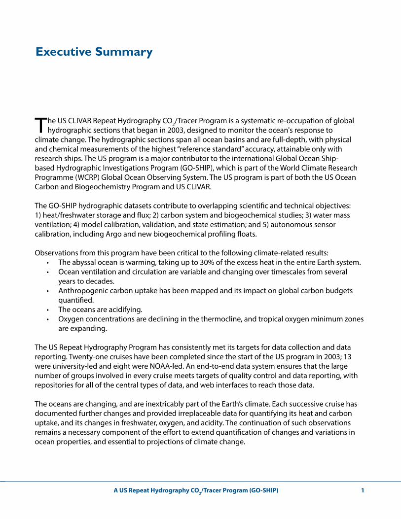
T he US CLIVAR Repeat Hydrography CO2/Tracer Program is a systematic re-occupation of global hydrographic sections that began in 2003, designed to monitor the ocean's response to

climate change. The hydrographic sections span all ocean basins and are full-depth, with physical and chemical measurements of the highest “reference standard” accuracy, attainable only with research ships. The US program is a major contributor to the international Global Ocean Ship-based Hydrographic Investigations Program (GO-SHIP), which is part of the World Climate Research Programme (WCRP) Global Ocean Observing System. The US program is part of both the US Ocean Carbon and Biogeochemistry Program and US CLIVAR.

The GO-SHIP hydrographic datasets contribute to overlapping scientific and technical objectives: 1) heat/freshwater storage and flux; 2) carbon system and biogeochemical studies; 3) water mass ventilation; 4) model calibration, validation, and state estimation; and 5) autonomous sensor calibration, including Argo and new biogeochemical profiling floats.

Observations from this program have been critical to the following climate-related results: • The abyssal ocean is warming, taking up to 30% of the excess heat in the entire Earth system.• Ocean ventilation and circulation are variable and changing over timescales from several

years to decades.• Anthropogenic carbon uptake has been mapped and its impact on global carbon budgets

quantified.• The oceans are acidifying.• Oxygen concentrations are declining in the thermocline, and tropical oxygen minimum zones

are expanding.

The US Repeat Hydrography Program has consistently met its targets for data collection and data reporting. Twenty-one cruises have been completed since the start of the US program in 2003; 13 were university-led and eight were NOAA-led. An end-to-end data system ensures that the large number of groups involved in every cruise meets targets of quality control and data reporting, with repositories for all of the central types of data, and web interfaces to reach those data.

The oceans are changing, and are inextricably part of the Earth’s climate. Each successive cruise has documented further changes and provided irreplaceable data for quantifying its heat and carbon uptake, and its changes in freshwater, oxygen, and acidity. The continuation of such observations remains a necessary component of the effort to extend quantification of changes and variations in ocean properties, and essential to projections of climate change.

A US Repeat Hydrography CO2/Tracer Program (GO-SHIP)2

kuhlenbr

Typewritten Text

This page intentionally left blank.

kuhlenbr

Typewritten Text

kuhlenbr

Typewritten Text


1 Introduction

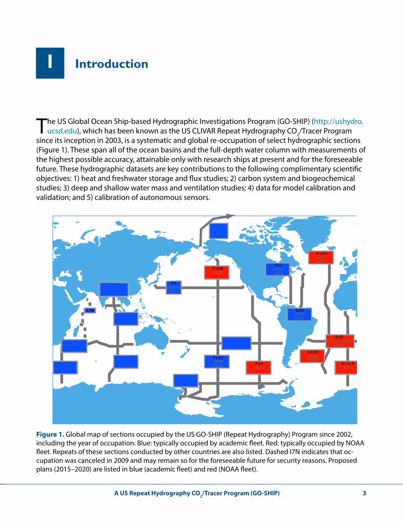
T he US Global Ocean Ship-based Hydrographic Investigations Program (GO-SHIP) (http://ushydro.ucsd.edu), which has been known as the US CLIVAR Repeat Hydrography CO2/Tracer Program

since its inception in 2003, is a systematic and global re-occupation of select hydrographic sections (Figure 1). These span all of the ocean basins and the full-depth water column with measurements of the highest possible accuracy, attainable only with research ships at present and for the foreseeable future. These hydrographic datasets are key contributions to the following complimentary scientific objectives: 1) heat and freshwater storage and flux studies; 2) carbon system and biogeochemical studies; 3) deep and shallow water mass and ventilation studies; 4) data for model calibration and validation; and 5) calibration of autonomous sensors.

2009, 20172003 (Japan)

2002 (UK) 2009, 2018

2019

ARC01(2005) 2015

2016

2016

I1E(WOCE 1995)

2016

2019

2020

20132004

2014

20032012

2003 (Japan)2011

20032013

2005P16S

P2

A20

A10

A2220032012

Figure 1. Global map of sections occupied by the US GO-SHIP (Repeat Hydrography) Program since 2002, including the year of occupation. Blue: typically occupied by academic fleet. Red: typically occupied by NOAA fleet. Repeats of these sections conducted by other countries are also listed. Dashed I7N indicates that oc-cupation was canceled in 2009 and may remain so for the foreseeable future for security reasons. Proposed plans (2015–2020) are listed in blue (academic fleet) and red (NOAA fleet).

http://ushydro.ucsd.edu



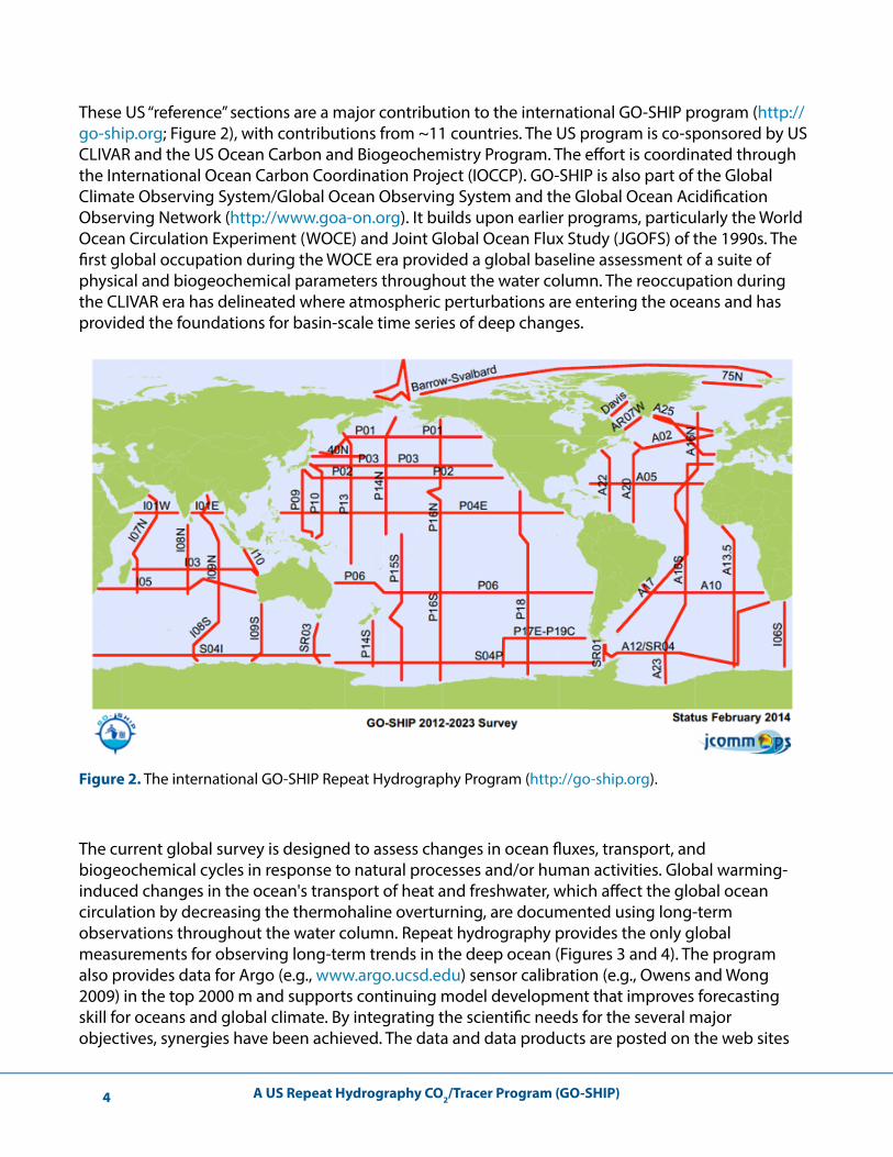
These US “reference” sections are a major contribution to the international GO-SHIP program (http://go-ship.org; Figure 2), with contributions from ~11 countries. The US program is co-sponsored by US CLIVAR and the US Ocean Carbon and Biogeochemistry Program. The effort is coordinated through the International Ocean Carbon Coordination Project (IOCCP). GO-SHIP is also part of the Global Climate Observing System/Global Ocean Observing System and the Global Ocean Acidification Observing Network (http://www.goa-on.org). It builds upon earlier programs, particularly the World Ocean Circulation Experiment (WOCE) and Joint Global Ocean Flux Study (JGOFS) of the 1990s. The first global occupation during the WOCE era provided a global baseline assessment of a suite of physical and biogeochemical parameters throughout the water column. The reoccupation during the CLIVAR era has delineated where atmospheric perturbations are entering the oceans and has provided the foundations for basin-scale time series of deep changes.

The current global survey is designed to assess changes in ocean fluxes, transport, and biogeochemical cycles in response to natural processes and/or human activities. Global warming-induced changes in the ocean's transport of heat and freshwater, which affect the global ocean circulation by decreasing the thermohaline overturning, are documented using long-term observations throughout the water column. Repeat hydrography provides the only global measurements for observing long-term trends in the deep ocean (Figures 3 and 4). The program also provides data for Argo (e.g., www.argo.ucsd.edu) sensor calibration (e.g., Owens and Wong 2009) in the top 2000 m and supports continuing model development that improves forecasting skill for oceans and global climate. By integrating the scientific needs for the several major objectives, synergies have been achieved. The data and data products are posted on the web sites

Figure 2. The international GO-SHIP Repeat Hydrography Program (http://go-ship.org).

http://go-ship.org

http://go-ship.org

www.argo.ucsd.edu

http://go-ship.org


for the CLIVAR and Carbon Hydrographic Data Office (CCHDO; http://cchdo.ucsd.edu/) and the Carbon Dioxide Information Analysis Center (CDIAC; http://cdiac.ornl.gov/oceans/), and the results are used for major assessments of the role of the ocean in mitigating climate change, research publications, atlases, and outreach materials. The products are used to develop and validate ocean biogeochemistry and circulation models.

The US component of GO-SHIP is co-funded by NOAA and the National Science Foundation (NSF) in support of the Ocean Carbon Observing Network of the Program Plan for Building a Sustained Observing Network for Climate (see Section 3.1). The sequence and timing for the sections (Figure 1) takes into consideration the program objectives, providing global coverage, and working with-in resource constraints. Other considerations are the timing of national and international research programs, including the focus of CLIVAR in the 2011–2014 time frame; the International Surface Ocean–Lower Atmosphere Study (SOLAS) Project, which emphasizes constraining the carbon uptake in the surface oceans; the open-ocean component of the NOAA Ocean Acidification Program; and the international Integrated Marine Biogeochemistry and Ecosystem Research (IMBER) Program. The US GO-SHIP sections are selected so that there is roughly a decade between occupations, which is optimal for detecting changes in ocean carbon inventory, and changes in deep freshwater and heat transport.

http://cchdo.ucsd.edu

http://cdiac.ornl.gov/oceans


kuhlenbr

Typewritten Text



2 Accomplishments

Over the last decade, GO-SHIP has resulted in major scientific discoveries that have significantly advanced our understanding of the roles of the ocean in climate change, carbon cycling, and

biogeochemical responses. These discoveries have been described in over 200 peer-reviewed journal publications and global syntheses, including the Regional Carbon Cycle Assessment and Processes (RECCAP) and the IPCC 5th Assessment Report. A few of the major research highlights are briefly described below.

2.1 Heat and salinity

2.1.a Abyssal ocean warming The variability in ocean heat storage on basin or sub-basin scales is caused by decadally varying atmospheric forcing; the significance of the amount of heat stored in the deep ocean has only become evident in the past several years. GO-SHIP currently provides the only global measurements of the changing temperature and salinity in the bottom half of the ocean volume, below the 2000 m profiling depth of the Argo array, and will likely continue to be the only source of the necessary, highly accurate deep ocean measurements for many years to come. Beginning with a comparison of two pairs of zonal hydrographic sections taken some 25 years apart (Roemmich and Wunsch 1984) in the North Atlantic, there has been ongoing documentation of the changing character of the ocean, from the surface to the bottom, based on these observations.

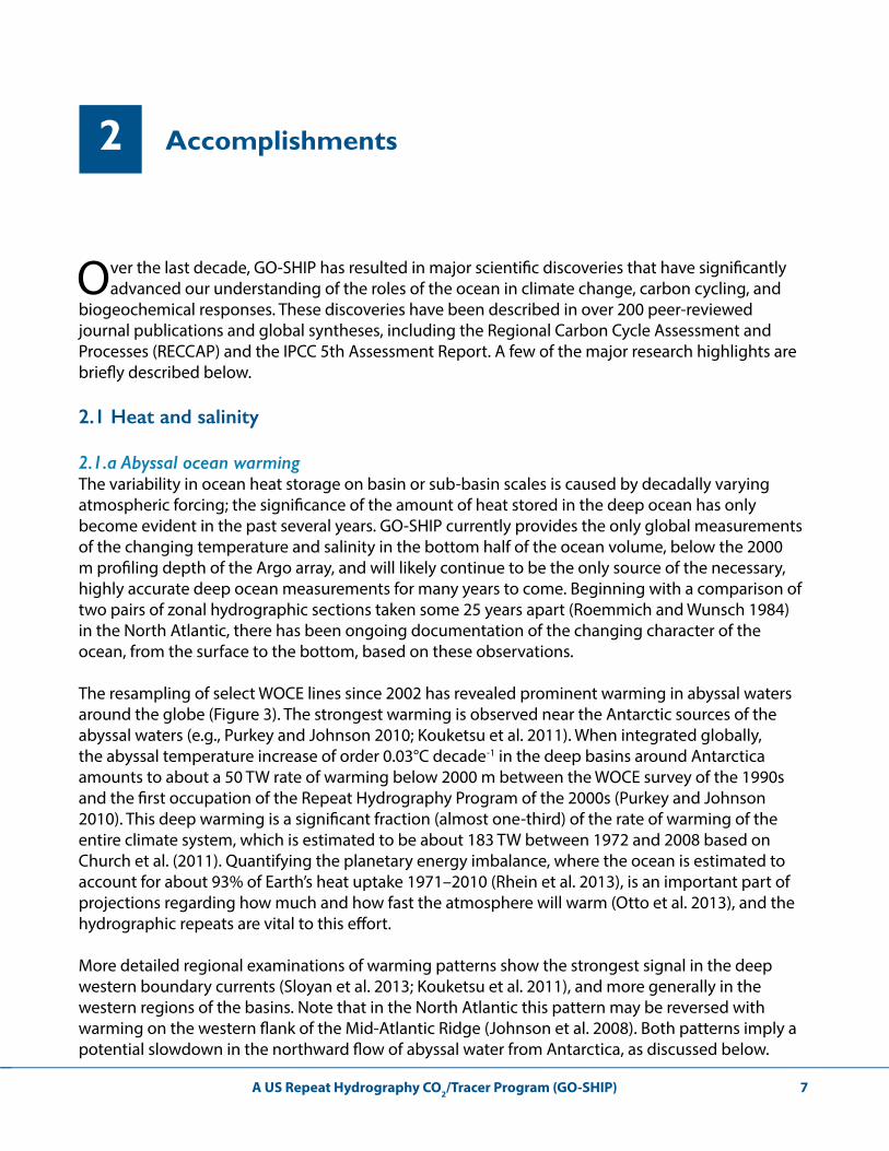
The resampling of select WOCE lines since 2002 has revealed prominent warming in abyssal waters around the globe (Figure 3). The strongest warming is observed near the Antarctic sources of the abyssal waters (e.g., Purkey and Johnson 2010; Kouketsu et al. 2011). When integrated globally, the abyssal temperature increase of order 0.03°C decade-1 in the deep basins around Antarctica amounts to about a 50 TW rate of warming below 2000 m between the WOCE survey of the 1990s and the first occupation of the Repeat Hydrography Program of the 2000s (Purkey and Johnson 2010). This deep warming is a significant fraction (almost one-third) of the rate of warming of the entire climate system, which is estimated to be about 183 TW between 1972 and 2008 based on Church et al. (2011). Quantifying the planetary energy imbalance, where the ocean is estimated to account for about 93% of Earth’s heat uptake 1971–2010 (Rhein et al. 2013), is an important part of projections regarding how much and how fast the atmosphere will warm (Otto et al. 2013), and the hydrographic repeats are vital to this effort.

More detailed regional examinations of warming patterns show the strongest signal in the deep western boundary currents (Sloyan et al. 2013; Kouketsu et al. 2011), and more generally in the western regions of the basins. Note that in the North Atlantic this pattern may be reversed with warming on the western flank of the Mid-Atlantic Ridge (Johnson et al. 2008). Both patterns imply a potential slowdown in the northward flow of abyssal water from Antarctica, as discussed below.


Figure 3. Rates of temperature change below 4000 m (colors, see key) in deep basins (thin gray lines) estimated from CLIVAR repeats of WOCE hydrographic sections (black lines). Basins where changes are not statistically different from zero at 95% confidence are stippled. Rhein et al. (2013) based on Purkey and Johnson (2010).

2.1.b Deep ocean freshwater changesAlthough the Argo profiling float array provides better temporal resolution of heat and freshwater storage in the upper ocean than repeat hydrography (e.g., Johnson and Lyman 2007; Durack and Wijffels 2010), at present, the GO-SHIP hydrographic repeat sections provide the only observations that allow continued investigation into changes in deep salinity on a global basis. Furthermore, Argo salinities require in situ calibration (against hydrography), hence GO-SHIP will remain necessary for validation/calibration for deep Argo as it is implemented over the next decade. GO-SHIP also provides tracer information that is independent of and complements salinity observations—for example, the oxygen changes observed over the past decade (see Section 2.4) that reflect changes in ventilation and freshwater sources.

A global assessment of freshwater storage change using hydrographic data has shown coherent large-scale patterns (Boyer et al. 2005; Bindoff et al. 2007) that have been more recently delineated by the upper ocean Argo profiling float network (Durack and Wijffels 2010). These changes appear consistent with the loss of freshwater from low latitudes, and its deposition at higher latitudes. Further, a zonal redistribution of freshwater from the saline Atlantic and Indian oceans to the fresher Pacific has been documented (Durack et al. 2012; Bindoff et al. 2007; IPCC 2013).

GO-SHIP repeat hydrography shows freshening in the Southern Hemisphere pycnocline, at levels shallower than Antarctic Intermediate Water (also in Helm et al. 2010). Salinity has increased in the


subtropical salinity maxima of the South Indian and South Atlantic oceans. Near-surface freshening occurred in the Pacific subtropical salinity maxima and throughout the tropical Atlantic surface waters. The Southern Hemisphere thermocline freshening is likely related to increased ventilation from the south, based on oxygen and chlorofluorocarbon (CFC) changes on the same sections.

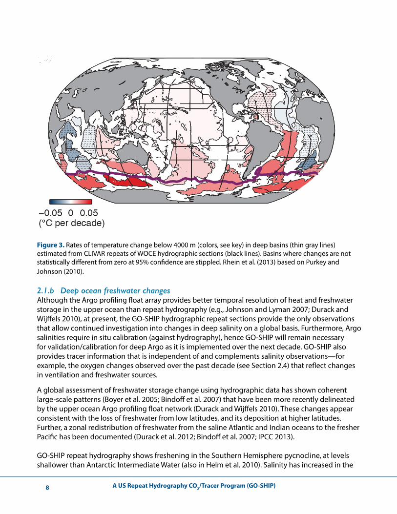
From GO-SHIP observations, an abyssal freshening equivalent to the addition of about 100 Gt year-1 of freshwater around Antarctica has been estimated for Antarctic Bottom Waters of θ < 0°C (Purkey and Johnson 2013), a significant fraction of the increase in ice sheet melt there in recent years (e.g., Rignot et al. 2008). The freshening rate is as large as 0.06 PSS-78 in the Ross Bottom Waters adjacent to the continental rise between 1992 and 2011, but smaller offshore (Swift and Orsi 2012). Similar freshening is found, again strongest in the newly formed bottom waters, offshore of the Adelie Lands to the west (Rintoul 2007). There is much less freshening in the bottom waters of the Weddell Sea (Purkey and Johnson 2013; Figure 4).

Figure 4. Rates of freshwater inventory change (colors, see key) owing to water-mass (θ-S) changes within Antarctic Bottom Water (θ < 0ºC) in deep basins (thin gray lines) estimated from CLIVAR/GO-SHIP repeats of WOCE hydrographic sections. Adapted from Purkey and Johnson (2013).

Abyssal changes in temperature and salinity, along with signaling changes in ventilation of the waters that fill much of the deep global ocean (Johnson 2008) and changes in the global meridional overturning circulation (MOC) discussed below, can also contribute to regional sea level rise (Purkey and Johnson 2013; Kouketsu et al. 2011).

2.2 Circulation and diffusivities

2.2.a Abyssal ocean circulation changesThe deep warming discussed in Section 2.1 corresponds to a contraction rate of about 8 Sv for Antarctic Bottom Waters of θ < 0°C (Purkey and Johnson 2012). This rate of disappearance is probably not directly translatable to a change in transport or ventilation rate, although it does


imply a reduction in ventilation. Investigations into the causes of this large change are ongoing. A reduction in CFC inventories in the abyssal waters of the Weddell Sea and Australian-Antarctic Basin over the last few decades (Huhn et al. 2013; Reed et al. submitted) certainly suggests a significant decrease in ventilation rates in that sector of the Southern Ocean.

This dramatic reduction in Antarctic Bottom Water volumes (roughly equivalent to a descent of the 0ºC potential isotherm of about 100 m decade-1) appears to be associated with a decadal reduction in northward flows of warmer, modified bottom waters of Antarctic origin through the South Pacific and Atlantic oceans (Kouketsu et al. 2011). The assimilation of WOCE and GO-SHIP repeat hydrographic sections into a model by these investigators estimates a slowdown of 0.7 Sv decade-1 in the South Pacific and 0.4 Sv decade-1 in the western South Atlantic from 1968 to 2005. The abyssal warming pattern in the South Pacific, with more warming at the western boundary (Sloyan et al. 2013), is consistent with this pattern through thermal wind.

Northern Hemisphere GO-SHIP results show a continuation of this slowdown distant from its origin. In the North Pacific, an inverse model analysis using repeat hydrography data from 1985 and 2005 suggests a decrease in northward bottom water transport of 1.5 Sv (Kouketsu et al. 2009). In the North Atlantic, analysis of five sections occupied across 24ºN between 1981 and 2010 suggests that northward flow of bottom water is reduced by order 1 Sv, although not monotonically (Frajka-Williams et al. 2011). This reduction of bottom-intensified northward flow over the Mid-Atlantic Ridge is consistent, again through thermal wind, with the deep pattern of warming on the western flank of the Mid-Atlantic Ridge and cooling west of that (Johnson et al. 2008).

While advective signatures of changes in the Antarctic Bottom Water would take many decades, perhaps centuries, to be measurable in temperature and salinity, planetary waves can carry signatures of such changes all the way to the North Pacific in a few decades, as demonstrated by analysis of a global data assimilation of repeat hydrographic data (Masuda et al. 2010).

2.2.b Transport analyses and changesVelocity analyses based on geostrophy and direct measurements provide transport estimates through direct calculations using station profiles, and through incorporation in inverse models and ocean state estimates. Basin-wide transport changes are difficult to compute using the sparse network of GO-SHIP sections, in comparison with the more complete WOCE coverage, which has been used repeatedly for basin- and global-scale inverse model circulation analyses (e.g., Ganachaud and Wunsch 2000; Reid 2003; Lumpkin and Speer 2007; Macdonald et al. 2009). Transport changes observed using GO-SHIP data have principally involved single transect comparisons, interpreted in terms of changes in ventilation in the upper ocean, MOC, and abyssal circulation (Section 2.2.a). Paired with observed changes in water mass properties that integrate over seasons and years, as opposed to quasi-synoptic transport analyses, the estimated transport changes may provide a compelling case for changing circulation, although great care is required in interpretation. The study of changes in North Atlantic overturning circulation using multiple occupations of the 24°N section over several decades (Bryden et al. 2005) provides a case in point; the continuous time series of transport that has been maintained shows large seasonal variability, and the trend reported based on the hydrographic sections falls within this variability (e.g., Hernández-Guerra et al. 2010). However, it should also be noted that oxygen changes that were also documented by Bryden et al. (2005) in their analysis of hydrographic repeats support the inferred decreasing trend.


Changing subtropical gyre transport in the Southern Hemisphere Indian Ocean was documented using repeats of the 32°S section, showing a strengthening from 1987 to 2002 (Palmer et al. 2004) that was consistent with increasing oxygen in the thermocline (McDonagh et al. 2005), hence increased ventilation. This increase has been associated with an increase in the Southern Annular Mode index, that is, an increase in strength of the westerly winds in the Southern Ocean. The difference in MOC transport assessed from the same repeats was within the large range of uncertainty, using both the CTD profiles with Lowered Acoustic Doppler Current Profiler (LADCP) velocities as an initial reference for the 2002 section (McDonagh et al. 2008). A subsequent 2009 repeat of the Indian Ocean section, analyzed in comparison with the 2002 section using an inverse model, indicates a slightly weaker overturning circulation in 2009 in the Indian Ocean; a coincident pair of repeats in the Pacific showed no significant change (Hernández-Guerra and Talley, in preparation).

To study changes in circulation in conjunction with water property changes on the circumpolar 32°S–20°S section completed in 2003–2004, Katsumata and Fukasawa (2011) take a different approach, given the issues with detecting decadal variations using synoptic sections. They use the hydrographic sections to describe changes in water properties, but then use two ocean general circulation models, one of them data-assimilating, to look at the circulation changes and their relationship to changes in atmospheric forcing, including the Southern Annular Mode.

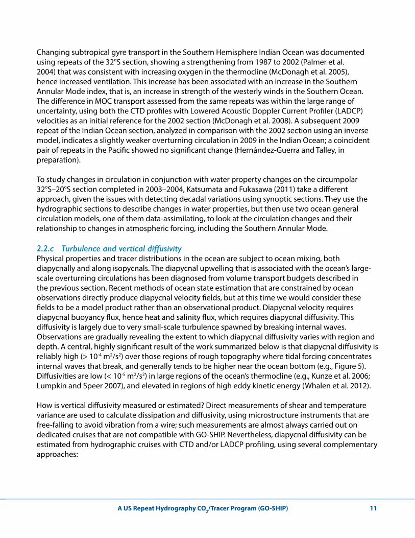
2.2.c Turbulence and vertical diffusivityPhysical properties and tracer distributions in the ocean are subject to ocean mixing, both diapycnally and along isopycnals. The diapycnal upwelling that is associated with the ocean’s large-scale overturning circulations has been diagnosed from volume transport budgets described in the previous section. Recent methods of ocean state estimation that are constrained by ocean observations directly produce diapycnal velocity fields, but at this time we would consider these fields to be a model product rather than an observational product. Diapycnal velocity requires diapycnal buoyancy flux, hence heat and salinity flux, which requires diapycnal diffusivity. This diffusivity is largely due to very small-scale turbulence spawned by breaking internal waves. Observations are gradually revealing the extent to which diapycnal diffusivity varies with region and depth. A central, highly significant result of the work summarized below is that diapycnal diffusivity is reliably high (> 10-4 m2/s2) over those regions of rough topography where tidal forcing concentrates internal waves that break, and generally tends to be higher near the ocean bottom (e.g., Figure 5). Diffusivities are low (< 10-5 m2/s2) in large regions of the ocean’s thermocline (e.g., Kunze et al. 2006; Lumpkin and Speer 2007), and elevated in regions of high eddy kinetic energy (Whalen et al. 2012).

How is vertical diffusivity measured or estimated? Direct measurements of shear and temperature variance are used to calculate dissipation and diffusivity, using microstructure instruments that are free-falling to avoid vibration from a wire; such measurements are almost always carried out on dedicated cruises that are not compatible with GO-SHIP. Nevertheless, diapycnal diffusivity can be estimated from hydrographic cruises with CTD and/or LADCP profiling, using several complementary approaches:


1. The most recent explosion of estimates of diapycnal diffusivity from hydrographic cruise data employs the so-called “finescale parameterization method,” which estimates internal wave vertical strain and vertical shear from CTD and LADCP profile data. The strain and shear are then related through an empirical parameterization to the local turbulence level due to internal waves and hence to energy dissipation and diapycnal diffusivity (Gregg 1989; Polzin et al. 1995; recent summary in Polzin et al. 2014). An example from Kunze et al. (2006) of a section at 32°S in the Indian Ocean using WOCE data is shown in Figure 5. In dynamically quiet regions away from boundaries and strong currents, available fine-structure parameterization methods are expected to be accurate to within about a factor of two when averaged over ~2000 m (Polzin et al. 1995, 2014). WOCE and repeat hydrography observations are being used to construct these parameterized diffusivity fields (e.g., Naveira Garabato et al. 2004; Sloyan 2005, 2006; Kunze et al. 2006; Huussen et al. 2012; Whalen et al. 2012; Sheen et al. 2013; Waterman et al. 2013; Waterhouse et al. 2014), revealing the large regional and vertical variability in the diffusivity field mentioned above. Such estimates, with growing contributions from the US GO-SHIP program, may contribute to new parameterizations of mixing in global-scale ocean circulation models, such as those recently developed by Palmer et al. (2007) and Melet et al. (2013).

2. CTD profiles, at their highest resolution, have been used to estimate vertical overturning length scales, or “Thorpe scales,” from which dissipation and diapycnal diffusivity can be estimated (e.g., Dillon 1982; Ferron et al. 1998). Sloyan et al. (2010) calculated Thorpe scale dissipation and diffusivity estimates in the upper ocean in the southeast Pacific from CTD observations and also a large free-fall XCTD dataset. CTD data are not ideal for these calculations, principally due to error arising from the ship motion and large rosette frame size (e.g., Polzin et al. 2014). Nevertheless, their broad observation base makes them a reasonable first step in an analysis.

3. Inverse models and other approaches to closed transport analyses use hydrographic section data to construct mass-balancing geostrophic velocity fields that include diapycnal transport between layers, from which the regionally averaged diapycnal diffusivity distribution can be inferred. Basin-wide inversions of WOCE hydrographic section data have produced multiple estimates of diffusivities (e.g., Robbins and Toole 1997; Ganachaud and Wunsch 2000; Lumpkin and Speer 2007; Macdonald et al. 2009). This approach is being continued with repeat hydrography section data (e.g., Huussen et al. 2012).


Figure 5. Diapycnal diffusivity κ along 32°S in the Indian Ocean, estimated from CTD and LADCP profiles (Kunze et al. 2006) using a finescale parameterization, representative of numerous recent studies (e.g., Polzin et al. 2014).

The future for continually improving vertical diffusivity estimates from repeat hydrography cruises is bright. Recent developments indicate that LADCP data can also be processed for vertical velocity and that finescale vertical velocity is highly correlated with turbulence and mixing levels, allowing the development of a new fine-structure parameterization method (Thurnherr 2011; Thurnherr et al. in preparation); data acquired from repeat hydrography cruises this year will be processed in this way. In a separate development, an experimental (Level 3) “chipod” program has been added to the US repeat hydrography sections, starting in 2013. Chipods measure temperature variance with much greater accuracy than a typical CTD; temperature variance can then be related to dissipation and diapycnal diffusivity (Moum and Nash 2009; Perlin and Moum 2012) more accurately than the finescale parameterization method. The Atlantic’s A16S chipod section has been completed successfully (Nash et al. 2014) and P16S, which also included chipod, was completed in May 2014.

2.3 Carbon

2.3.a InorganiccarboninventoriesandfluxesThe global ocean has continued to take up a substantial fraction of the anthropogenic CO2 emissions since the WOCE/JGOFS era, thereby constituting a major mediator of global climate change. Simulations with both general ocean circulation models and data-constrained models suggest that the ocean has taken up approximately 37 Pg C of this anthropogenic CO2 between 1994 and 2010 (Khatiwala et al. 2012), which amounts to about 27% of the total anthropogenic CO2 emissions over that time period. This uptake has increased the total inventory of anthropogenic CO2 from about 118 ± 20 Pg C in 1994 to about 155 ± 26 Pg C in 2010 (Khatiwala et al. 2012). However, this globally critical estimate is based on numerical techniques using transient tracers and has so far not been independently verified using ocean carbon observations. The GO-SHIP repeat occupations of many of the lines measured during the WOCE/JGOFS era permit us now to do so, and to provide a global synthesis of observation-based uptake estimates.


The underlying principle to assess the change in storage of anthropogenic CO2 (Cant) is to determine the change in Cant concentration between two occupations. This calculation is not trivial, however, as this change is just part of the total change in dissolved inorganic carbon (DIC) between two occupations, requiring methods to disentangle Cant from the often much larger changes in the natural carbon content due to changes in ventilation and remineralization, for example (Sabine and Tanhua 2010). Over the last few years, several methods have been developed and tested, permitting the community to overcome much of this challenge (e.g., the eMLR method (Friis et al. 2005)). More recently, the eMLR has been extended to permit not only the estimation of Cant along exact repeats, but also globally (Clement and Gruber 2014).

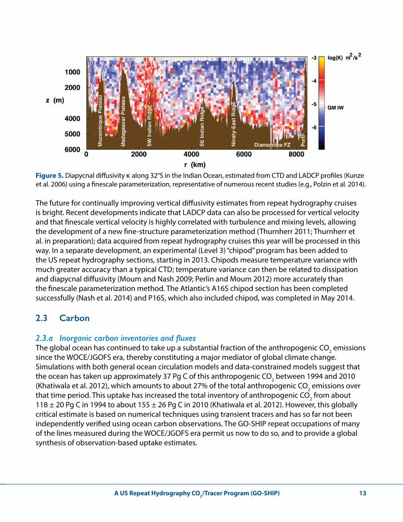
Preliminary global-scale results of the Cant storage rate from this modified eMLR method (Gruber et al. 2014) show a distribution that largely corresponds to the expectations based on the inventory of Cant and the observed increase in atmospheric CO2 (Figure 6), with an integral for global carbon uptake between 1994 and 2006 that is somewhat lower than the model-derived uptake, i.e., about 35 Pg C rather than 37 Pg C. However, the large uncertainties of this preliminary estimate preclude any statement with regard to the significance of this difference. A comparison of this preliminary global-scale estimate with published estimates along the repeated lines reveals also agreements and important differences, highlighting the need to further refine the methods.

Figure 6. Inorganic carbon-based estimates of the anthropogenic CO2 (Cant) storage rate (mol m-2 yr-1) between 1994 and 2006 determined from the GO-SHIP (CLIVAR) Repeat Hydrography Program. These are preliminary results (Gruber et al. 2014) based on a modified eMLR method (Clement and Gruber 2014).


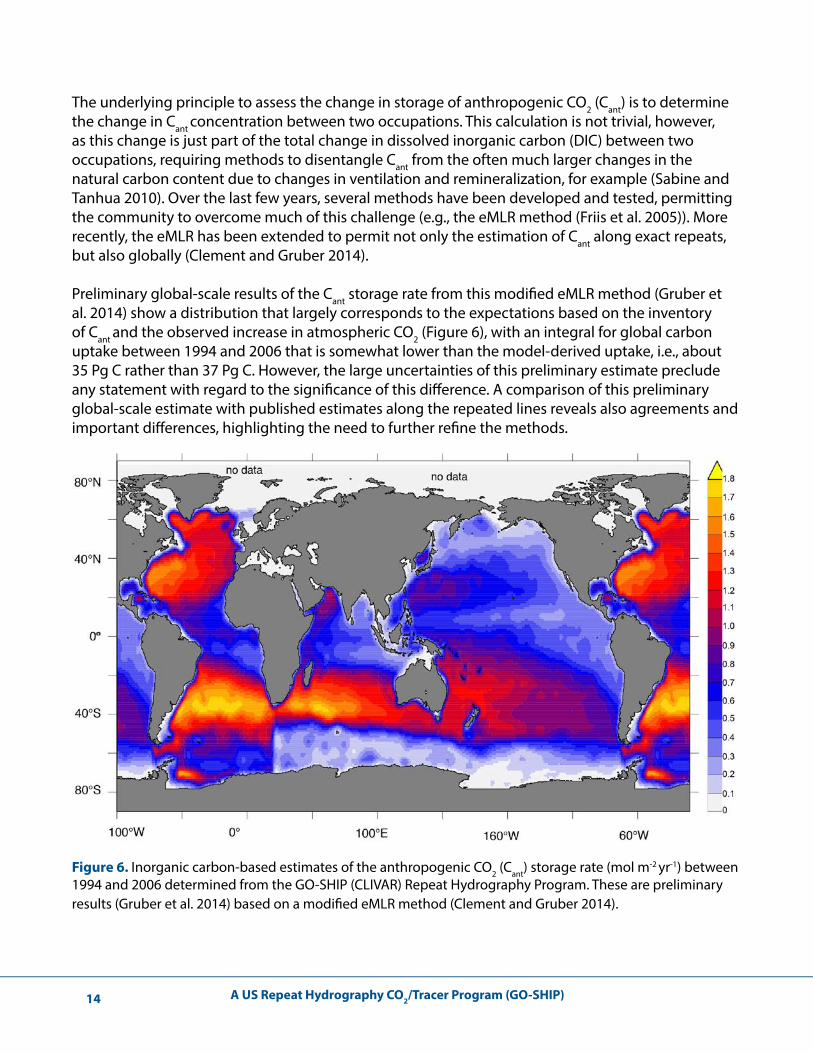
Some of the differences might also be real, reflecting temporal variations in the storage rate. The global-scale estimate represents the time-mean over the ~1994 to ~2007 period, while the individual estimates represent storage rates of specific intervals. For example, substantial temporal differences in storage rates have been observed on decadal and sub-decadal time scales (Wanninkhof et al. 2010, 2013a; Sabine and Tanhua 2010; Khatiwala et al. 2012) (Figure 7). Pérez et al. (2010) found that the Cant storage rate in the North Atlantic was dependent on the North Atlantic Oscillation (NAO), with highest Cant storage rates occurring during the positive phase of NAO and low storage rates during the negative phase of NAO. Furthermore, Pérez et al. (2013) showed a decrease in uptake from 1990 to 2006 that was attributed to weakening of the MOC. In the Pacific Ocean, there are higher Cant storage rates in the South Pacific as compared with the North Pacific (Murata et al. 2007; Sabine et al. 2008). In the Indian Ocean, the largest Cant storage rates are observed south of the equator where Cant increases have been observed to 1800 m (Murata et al. 2010; Álvarez et al. 2011). A number of studies that used observations from WOCE/GO-SHIP lines have indicated that the Southern Ocean may be responsible for as much as 30–40% of the global Cant uptake (e.g., Gruber et al. 2009; Khatiwala et al. 2009). There is still debate as to whether this uptake is stored or exported (Sabine et al. 2004; van Heuven et al. 2011) and in what water masses (e.g., Gruber et al. 1996; Sabine et al. 2004; van Heuven et al. 2011; Pardo et al. 2014), and both carbon parameters and other tracers (e.g., CFCs, CCl4 and 39Ar) from these cruises are being used to investigate the possibilities.

Figure 7. Decadal storage rates of Cant (mol m-2 yr-1) for the three ocean basins (left to right: Atlantic, Pacific, and Indian Oceans) as observed from repeat hydrography cruises. The horizontal lines depict the measurement intervals bracketed by repeat hydrography cruises. Measurements for the Northern Hemisphere are drawn as solid lines, the tropics as dash-dotted lines, and dashed lines for the Southern Hemisphere; the color schemes refer to different studies. Estimates of uncertainties are shown as vertical bars with matching colors along the right axes. The solid black line represents the basin average storage rate using Green’s function (from Khatiwala et al. 2012).

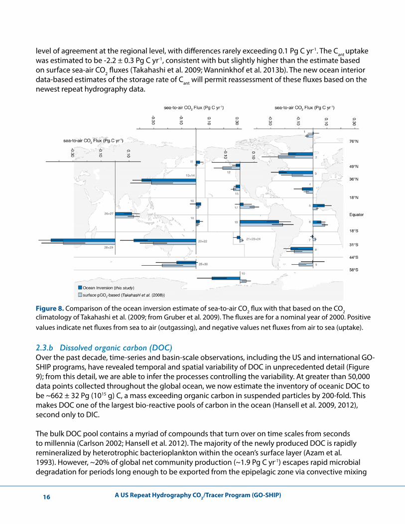
Ocean interior carbon observations also provide an important constraint on the air-sea CO2 fluxes. Gloor et al. (2003) demonstrated that it is possible to use inorganic carbon observations from the ocean interior to determine the net sea-air CO2 flux of both natural and anthropogenic CO2 through an ocean inversion procedure, provided one knows the ocean’s circulation and mixing well. Using a series of more than 10 general circulation models, Gruber et al. (2009) used an ensemble approach to overcome this issue, and using inorganic carbon data from the WOCE/JGOFS, augmented with new data from the CLIVAR era, they estimated the net sea-air flux of CO2 over 23 regions (Figure 8; Gruber et al. 2009). The comparison of these ocean interior carbon-based sea-air CO2 fluxes with those inferred from surface ocean pCO2 measurements (Takahashi et al. 2009) revealed a remarkable


level of agreement at the regional level, with differences rarely exceeding 0.1 Pg C yr-1. The Cant uptake was estimated to be -2.2 ± 0.3 Pg C yr-1, consistent with but slightly higher than the estimate based on surface sea-air CO2 fluxes (Takahashi et al. 2009; Wanninkhof et al. 2013b). The new ocean interior data-based estimates of the storage rate of Cant will permit reassessment of these fluxes based on the newest repeat hydrography data.

Figure 8. Comparison of the ocean inversion estimate of sea-to-air CO2 flux with that based on the CO2 climatology of Takahashi et al. (2009; from Gruber et al. 2009). The fluxes are for a nominal year of 2000. Positive values indicate net fluxes from sea to air (outgassing), and negative values net fluxes from air to sea (uptake).

2.3.b Dissolved organic carbon (DOC) Over the past decade, time-series and basin-scale observations, including the US and international GO-SHIP programs, have revealed temporal and spatial variability of DOC in unprecedented detail (Figure 9); from this detail, we are able to infer the processes controlling the variability. At greater than 50,000 data points collected throughout the global ocean, we now estimate the inventory of oceanic DOC to be ~662 ± 32 Pg (1015 g) C, a mass exceeding organic carbon in suspended particles by 200-fold. This makes DOC one of the largest bio-reactive pools of carbon in the ocean (Hansell et al. 2009, 2012), second only to DIC.

The bulk DOC pool contains a myriad of compounds that turn over on time scales from seconds to millennia (Carlson 2002; Hansell et al. 2012). The majority of the newly produced DOC is rapidly remineralized by heterotrophic bacterioplankton within the ocean’s surface layer (Azam et al. 1993). However, ~20% of global net community production (~1.9 Pg C yr-1) escapes rapid microbial degradation for periods long enough to be exported from the epipelagic zone via convective mixing


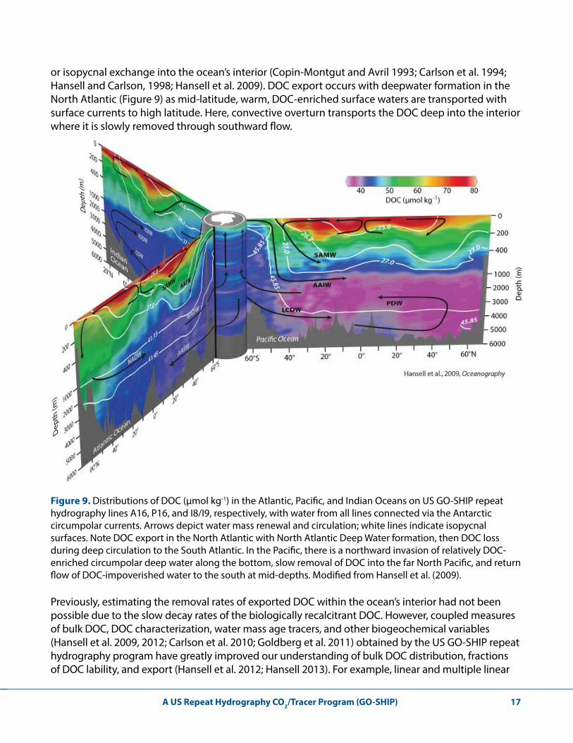
or isopycnal exchange into the ocean’s interior (Copin-Montgut and Avril 1993; Carlson et al. 1994; Hansell and Carlson, 1998; Hansell et al. 2009). DOC export occurs with deepwater formation in the North Atlantic (Figure 9) as mid-latitude, warm, DOC-enriched surface waters are transported with surface currents to high latitude. Here, convective overturn transports the DOC deep into the interior where it is slowly removed through southward flow.

Figure 9. Distributions of DOC (µmol kg-1) in the Atlantic, Pacific, and Indian Oceans on US GO-SHIP repeat hydrography lines A16, P16, and I8/I9, respectively, with water from all lines connected via the Antarctic circumpolar currents. Arrows depict water mass renewal and circulation; white lines indicate isopycnal surfaces. Note DOC export in the North Atlantic with North Atlantic Deep Water formation, then DOC loss during deep circulation to the South Atlantic. In the Pacific, there is a northward invasion of relatively DOC-enriched circumpolar deep water along the bottom, slow removal of DOC into the far North Pacific, and return flow of DOC-impoverished water to the south at mid-depths. Modified from Hansell et al. (2009).

Previously, estimating the removal rates of exported DOC within the ocean’s interior had not been possible due to the slow decay rates of the biologically recalcitrant DOC. However, coupled measures of bulk DOC, DOC characterization, water mass age tracers, and other biogeochemical variables (Hansell et al. 2009, 2012; Carlson et al. 2010; Goldberg et al. 2011) obtained by the US GO-SHIP repeat hydrography program have greatly improved our understanding of bulk DOC distribution, fractions of DOC lability, and export (Hansell et al. 2012; Hansell 2013). For example, linear and multiple linear


regression models applied to pairwise measurements of DOC and CFC-12 ventilation age, retrieved from major water masses within the main thermocline and North Atlantic Deep Water (A16, A20, A22), allow estimates of decay rates for exported DOC ranging from 0.13 to 0.94 µmol kg-1 yr-1, with higher DOC concentrations driving higher rates. Comparing the change in DOC to change in oxygen in the same water masses suggests that DOC oxidation contributes 5 to 29% of the apparent oxygen utilization in the deep water masses of the North Atlantic (Carlson et al. 2010).

Measurements of carbohydrate and dissolved combined neutral sugar (DCNS) concentrations allow us to further assess the change in chemical character along meridional transects in the North Atlantic (A20) and South Pacific (P16S). As microbes remineralize dissolved organic matter (DOM) they preferentially remove the most labile components of DOM such as carbohydrates and DCNS, leaving behind more recalcitrant components. Tracking the change in DCNS and the change in the mole fraction of the individual neutral sugars within the DCNS pool relative to change in total DOC allows one to assess the diagenetic alteration of DOM over depth and through time (Skoog and Benner 1997; Kaiser and Benner 2009; Goldberg et al. 2010). Data collected from the US GO-SHIP Repeat Hydrography Program reveal systematic diagenetic patterns of DOM across ocean basins (Goldberg et al. 2011), providing further insight of the roles that stratification, ventilation, export, and subsequent remineralization play in DOM quality (Goldberg et al. 2010).

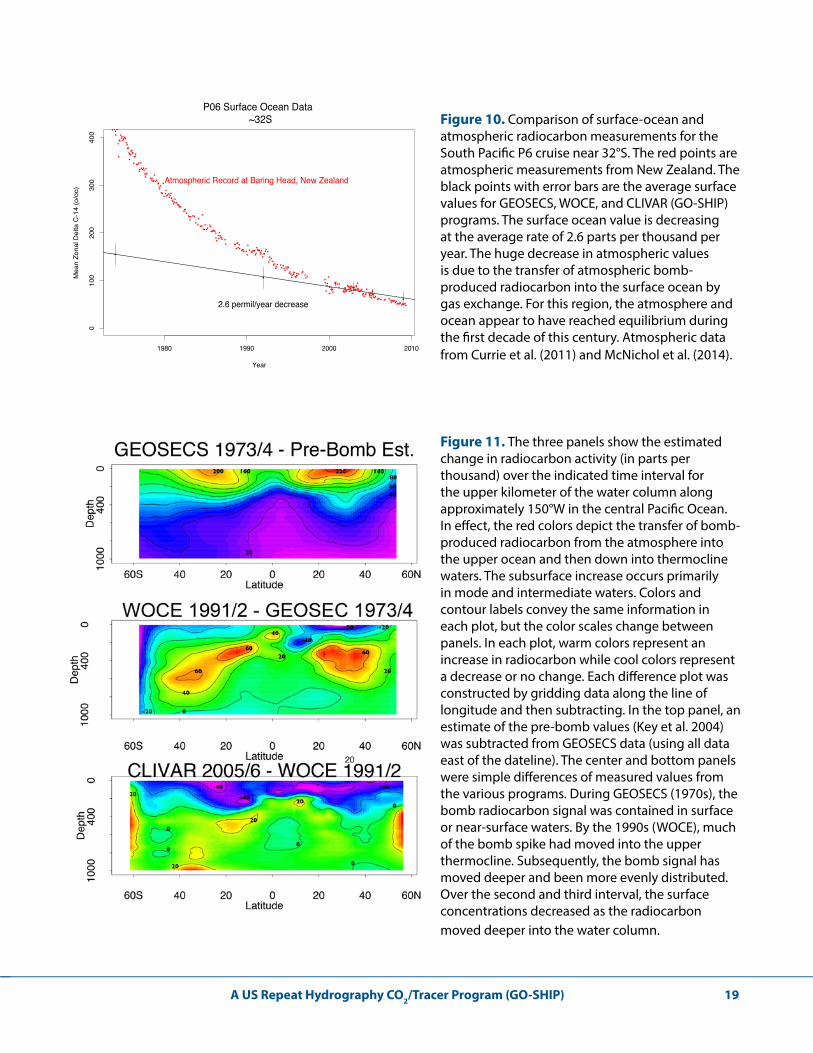
2.3.c RadiocarbonOceanic radiocarbon integrates the combined influences of air-sea gas exchange, ventilation, and mixing processes over longer time scales than for typical inorganic carbon. Improved measurement technology has reduced sample size requirements by a factor of 1000 relative to the initial high-quality survey (GEOSECS, mid-1970s) and measurement precision has improved by a factor of 2. GEOSECS was followed by TTO (Transient Tracers in the Ocean) and SAVE (South Atlantic Ventilation Experiment) in the Atlantic and then by the WOCE and GO-SHIP programs globally. The combined data have proven extremely valuable because, like anthropogenic CO2, the distribution of radiocarbon is transient. For radiocarbon, the decadal-scale change is due to atmospheric testing of nuclear weapons during the 1950s and 1960s. The bomb radiocarbon spike was sufficiently large to be easily measured as it moved from the atmosphere to the upper ocean and finally toward the abyss. Key et al. (2004) produced the first global 3-D maps of the distribution of measured, background, and bomb-produced radiocarbon. These were then integrated to yield inventories. Subsequently, the maps and inventories have been used for many investigations ranging from global mean air-sea exchange rates for CO2 to calibration of global ocean general circulation models to ocean ventilation rates. The GO-SHIP program has extended the time series and additionally has allowed us to monitor the bomb spike as it is mixed into the ocean. Figure 10 summarizes the transfer of the atmospheric bomb signal into the surface ocean for data collected on or near 30°S in the Pacific Ocean. Figure 11, showing data collected along 150°W in the central Pacific, clearly demonstrates the penetration of that signal as it moves down into the ocean. It is important to note that the change indicated in Figure 11 is large relative to our measurement capability. Such along-section changes have been described in several papers (Jenkins et al. 2010) and will be globally summarized once the data synthesis product GLODAPv2 is released (Olsen et al. 2014).


Figure 10. Comparison of surface-ocean and atmospheric radiocarbon measurements for the South Pacific P6 cruise near 32°S. The red points are atmospheric measurements from New Zealand. The black points with error bars are the average surface values for GEOSECS, WOCE, and CLIVAR (GO-SHIP) programs. The surface ocean value is decreasing at the average rate of 2.6 parts per thousand per year. The huge decrease in atmospheric values is due to the transfer of atmospheric bomb-produced radiocarbon into the surface ocean by gas exchange. For this region, the atmosphere and ocean appear to have reached equilibrium during the first decade of this century. Atmospheric data from Currie et al. (2011) and McNichol et al. (2014).

Figure 11. The three panels show the estimated change in radiocarbon activity (in parts per thousand) over the indicated time interval for the upper kilometer of the water column along approximately 150°W in the central Pacific Ocean. In effect, the red colors depict the transfer of bomb-produced radiocarbon from the atmosphere into the upper ocean and then down into thermocline waters. The subsurface increase occurs primarily in mode and intermediate waters. Colors and contour labels convey the same information in each plot, but the color scales change between panels. In each plot, warm colors represent an increase in radiocarbon while cool colors represent a decrease or no change. Each difference plot was constructed by gridding data along the line of longitude and then subtracting. In the top panel, an estimate of the pre-bomb values (Key et al. 2004) was subtracted from GEOSECS data (using all data east of the dateline). The center and bottom panels were simple differences of measured values from the various programs. During GEOSECS (1970s), the bomb radiocarbon signal was contained in surface or near-surface waters. By the 1990s (WOCE), much of the bomb spike had moved into the upper thermocline. Subsequently, the bomb signal has moved deeper and been more evenly distributed. Over the second and third interval, the surface concentrations decreased as the radiocarbon moved deeper into the water column.

•

••

•

P06 Surface Ocean Data ~32S

Year

Mea

n Zo

nal D

elta

C-1

4 (o

/oo)

1980 1990 2000 2010

010

020

030

040

0

2.6 permil/year decrease

•••••

•

•

•••••••••••••••

•••••••

••••••••••••••••

••• •••••

••••••••••

•

••••••••••••••••••••• ••••••••••••

••••

•••••••••••••••••••••••• •••

••••••••••••••••••••

•••••••••••••••••••••••• •••••••••••••••

•••••••• ••••• ••••••••••••••

••••••• •••••••••••••••••••••••••••••••

••••••••••••

•••••••••••••••••••• •• ••••••••••••••••••••

Atmospheric Record at Baring Head, New Zealand


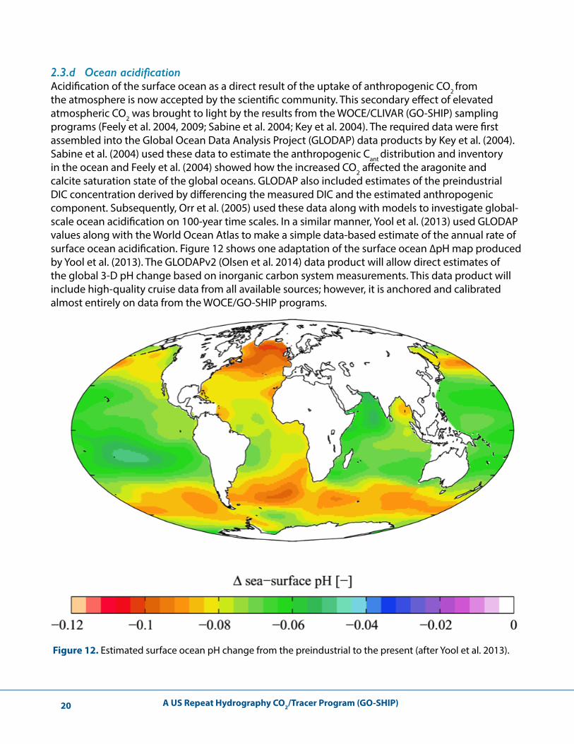
2.3.d OceanacidificationAcidification of the surface ocean as a direct result of the uptake of anthropogenic CO2 from the atmosphere is now accepted by the scientific community. This secondary effect of elevated atmospheric CO2 was brought to light by the results from the WOCE/CLIVAR (GO-SHIP) sampling programs (Feely et al. 2004, 2009; Sabine et al. 2004; Key et al. 2004). The required data were first assembled into the Global Ocean Data Analysis Project (GLODAP) data products by Key et al. (2004). Sabine et al. (2004) used these data to estimate the anthropogenic Cant distribution and inventory in the ocean and Feely et al. (2004) showed how the increased CO2 affected the aragonite and calcite saturation state of the global oceans. GLODAP also included estimates of the preindustrial DIC concentration derived by differencing the measured DIC and the estimated anthropogenic component. Subsequently, Orr et al. (2005) used these data along with models to investigate global-scale ocean acidification on 100-year time scales. In a similar manner, Yool et al. (2013) used GLODAP values along with the World Ocean Atlas to make a simple data-based estimate of the annual rate of surface ocean acidification. Figure 12 shows one adaptation of the surface ocean ∆pH map produced by Yool et al. (2013). The GLODAPv2 (Olsen et al. 2014) data product will allow direct estimates of the global 3-D pH change based on inorganic carbon system measurements. This data product will include high-quality cruise data from all available sources; however, it is anchored and calibrated almost entirely on data from the WOCE/GO-SHIP programs.

Figure 12. Estimated surface ocean pH change from the preindustrial to the present (after Yool et al. 2013).


2.4 Ocean ventilation: Oxygen

A major discovery over the last two decades has been systematic and large changes in oxygen, mostly reductions, documented through GO-SHIP repeat hydrography and local station time series. The oxygen changes are a clear indicator of large-scale changes in ventilation, solubility, and possibly remineralization, which can impact ecosystem health. While some of the observed oxygen changes could be due to changes in biology, the consensus based on modeling studies (e.g., Deutsch et al. 2005) and correlations with physical forcing such as the NAO (Johnson and Gruber 2007) is that physical changes usually predominate. Combination of oxygen data with transient tracer data provides further evidence regarding the time scales at which the ventilation changes occur (see Section 2.5). Combination of carbon data (e.g., Sabine et al. 2008) with pH data (e.g., Byrne et al. 2010) has allowed for the determination of separate DIC/pH changes along repeat sections into anthropogenic and ventilation components, including their respective effects on carbon storage and ocean acidification.

Oxygen decline is found most consistently in the oxygen minimum zones of the tropical Pacific, Atlantic, and Indian oceans, as well as in the subpolar North Pacific (Stramma et al. 2010, 2012; Keeling et al. 2010; Keeling and Manning 2014). The trend in the North Pacific is based on a >50-year time series of oxygen data at Ocean Station P, which shows large bi-decadal cycles on top of the smaller long-term trend (0.39–0.70 μmol kg-1 yr-1; Whitney et al. 2007). The repeat hydrography cruises have been instrumental in determining the spatial extent of the decadal-scale variations that extend into the subtropics (e.g., Emerson et al. 2004; Mecking et al. 2008) and are observed in all oceans as a result of changes in surface forcing (McDonagh et al. 2005; Johnson and Gruber 2007; Talley 2009).

Repeat hydrography data suggest multi-decadal changes. At 32°S in the Indian Ocean, McDonagh et al. (2005) found a substantial increase in oxygen from 1987 to 2002, reversing an oxygen decline observed earlier (Bindoff and McDougall 2000). An oxygen increase also occurred over similar time periods along the 30ºS repeat sections in the Pacific and Atlantic oceans (Talley 2009). This oxygenation of the subtropical thermocline likely resulted from increased ventilation due to spin-up of the Southern Hemisphere gyres, documented at least for the Pacific Ocean based on dynamic height changes (Roemmich et al. 2007). The most recent 2009 repeat of the I5 section, however, indicates yet another reversal in gyre conditions with oxygen decreasing (Figure 13; Mecking et al. 2012) in response to natural decadal variability as well as anthropogenic climate change (Kobayashi et al. 2012).

The deoxygenation measured in the open-ocean thermocline on repeat hydrography cruises over the past two decades is consistent with the expectation that warmer waters will hold less dissolved oxygen (solubility effect), and that warming-induced stratification leads to a decrease in the transport of dissolved oxygen from surface to subsurface waters (stratification effect) (Matear and Hirst 2003; Deutsch et al. 2005; Frölicher et al. 2009). About 15% of the oxygen decline between 1970 and 1990 can be explained by warming, while the remainder by increased stratification (Helm et al. 2011).


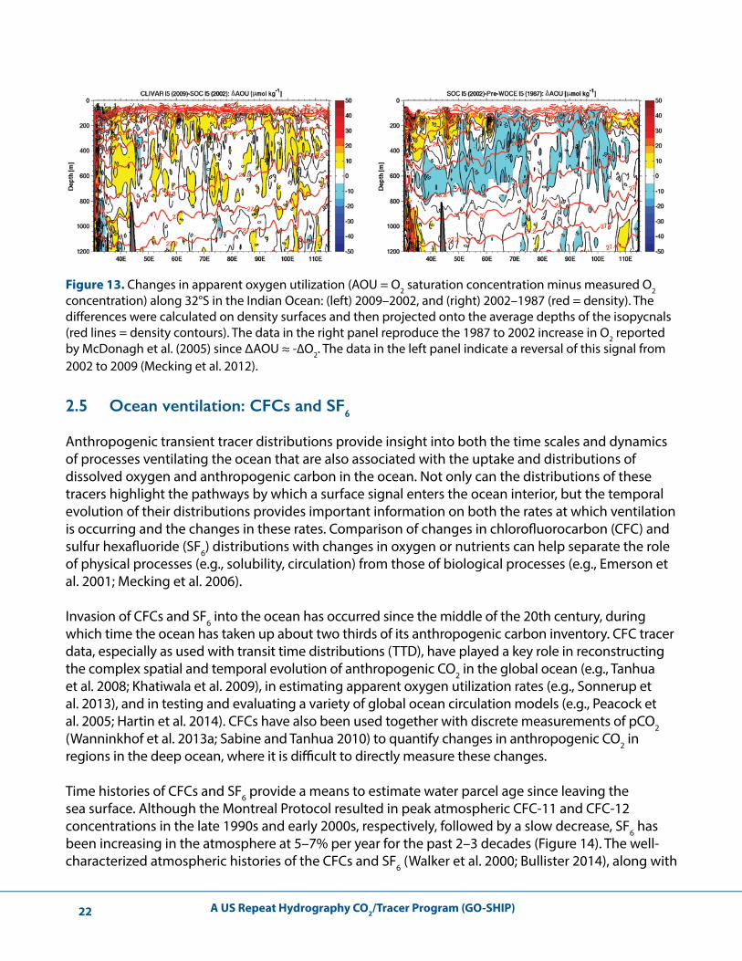
Figure 13. Changes in apparent oxygen utilization (AOU = O2 saturation concentration minus measured O2 concentration) along 32°S in the Indian Ocean: (left) 2009–2002, and (right) 2002–1987 (red = density). The differences were calculated on density surfaces and then projected onto the average depths of the isopycnals (red lines = density contours). The data in the right panel reproduce the 1987 to 2002 increase in O2 reported by McDonagh et al. (2005) since ΔAOU ≈ -∆O2. The data in the left panel indicate a reversal of this signal from 2002 to 2009 (Mecking et al. 2012).

2.5 Ocean ventilation: CFCs and SF6

Anthropogenic transient tracer distributions provide insight into both the time scales and dynamics of processes ventilating the ocean that are also associated with the uptake and distributions of dissolved oxygen and anthropogenic carbon in the ocean. Not only can the distributions of these tracers highlight the pathways by which a surface signal enters the ocean interior, but the temporal evolution of their distributions provides important information on both the rates at which ventilation is occurring and the changes in these rates. Comparison of changes in chlorofluorocarbon (CFC) and sulfur hexafluoride (SF6) distributions with changes in oxygen or nutrients can help separate the role of physical processes (e.g., solubility, circulation) from those of biological processes (e.g., Emerson et al. 2001; Mecking et al. 2006).

Invasion of CFCs and SF6 into the ocean has occurred since the middle of the 20th century, during which time the ocean has taken up about two thirds of its anthropogenic carbon inventory. CFC tracer data, especially as used with transit time distributions (TTD), have played a key role in reconstructing the complex spatial and temporal evolution of anthropogenic CO2 in the global ocean (e.g., Tanhua et al. 2008; Khatiwala et al. 2009), in estimating apparent oxygen utilization rates (e.g., Sonnerup et al. 2013), and in testing and evaluating a variety of global ocean circulation models (e.g., Peacock et al. 2005; Hartin et al. 2014). CFCs have also been used together with discrete measurements of pCO2 (Wanninkhof et al. 2013a; Sabine and Tanhua 2010) to quantify changes in anthropogenic CO2 in regions in the deep ocean, where it is difficult to directly measure these changes.

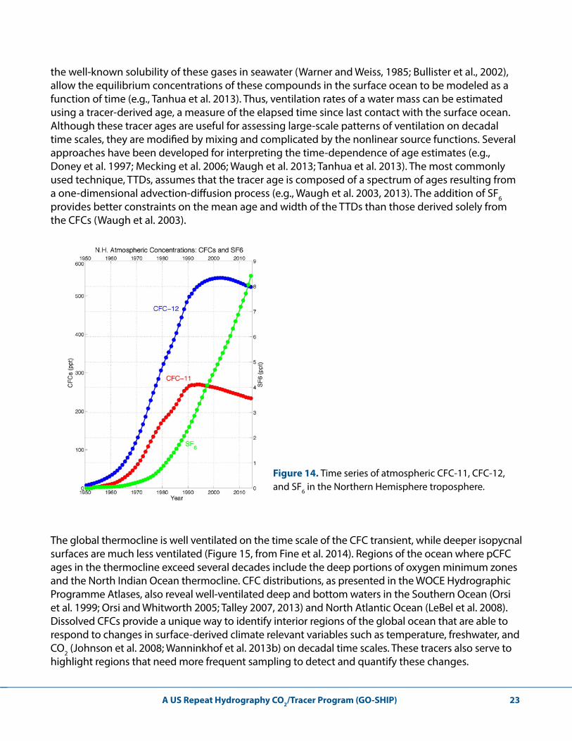
Time histories of CFCs and SF6 provide a means to estimate water parcel age since leaving the sea surface. Although the Montreal Protocol resulted in peak atmospheric CFC-11 and CFC-12 concentrations in the late 1990s and early 2000s, respectively, followed by a slow decrease, SF6 has been increasing in the atmosphere at 5–7% per year for the past 2–3 decades (Figure 14). The well-characterized atmospheric histories of the CFCs and SF6 (Walker et al. 2000; Bullister 2014), along with


the well-known solubility of these gases in seawater (Warner and Weiss, 1985; Bullister et al., 2002), allow the equilibrium concentrations of these compounds in the surface ocean to be modeled as a function of time (e.g., Tanhua et al. 2013). Thus, ventilation rates of a water mass can be estimated using a tracer-derived age, a measure of the elapsed time since last contact with the surface ocean. Although these tracer ages are useful for assessing large-scale patterns of ventilation on decadal time scales, they are modified by mixing and complicated by the nonlinear source functions. Several approaches have been developed for interpreting the time-dependence of age estimates (e.g., Doney et al. 1997; Mecking et al. 2006; Waugh et al. 2013; Tanhua et al. 2013). The most commonly used technique, TTDs, assumes that the tracer age is composed of a spectrum of ages resulting from a one-dimensional advection-diffusion process (e.g., Waugh et al. 2003, 2013). The addition of SF6 provides better constraints on the mean age and width of the TTDs than those derived solely from the CFCs (Waugh et al. 2003).

Figure 14. Time series of atmospheric CFC-11, CFC-12, and SF6 in the Northern Hemisphere troposphere.

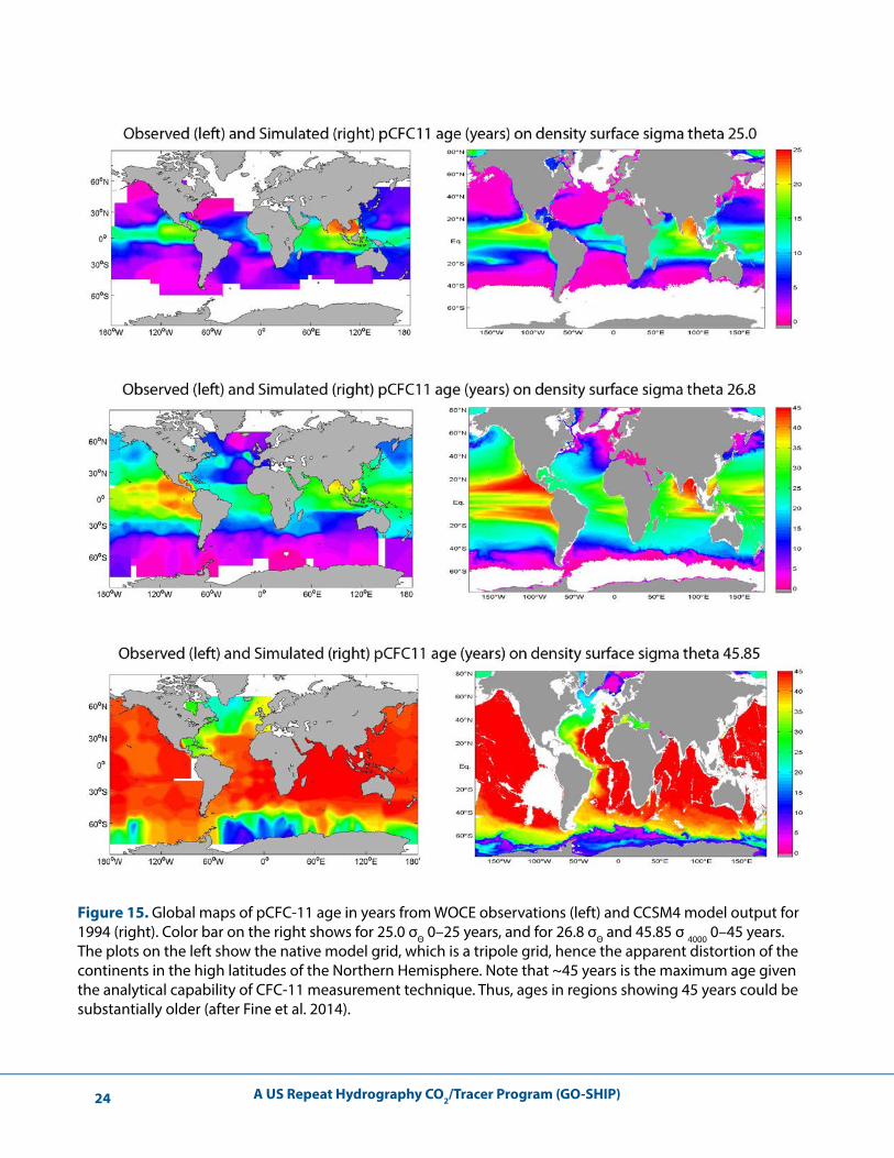
The global thermocline is well ventilated on the time scale of the CFC transient, while deeper isopycnal surfaces are much less ventilated (Figure 15, from Fine et al. 2014). Regions of the ocean where pCFC ages in the thermocline exceed several decades include the deep portions of oxygen minimum zones and the North Indian Ocean thermocline. CFC distributions, as presented in the WOCE Hydrographic Programme Atlases, also reveal well-ventilated deep and bottom waters in the Southern Ocean (Orsi et al. 1999; Orsi and Whitworth 2005; Talley 2007, 2013) and North Atlantic Ocean (LeBel et al. 2008). Dissolved CFCs provide a unique way to identify interior regions of the global ocean that are able to respond to changes in surface-derived climate relevant variables such as temperature, freshwater, and CO2 (Johnson et al. 2008; Wanninkhof et al. 2013b) on decadal time scales. These tracers also serve to highlight regions that need more frequent sampling to detect and quantify these changes.


Figure 15. Global maps of pCFC-11 age in years from WOCE observations (left) and CCSM4 model output for 1994 (right). Color bar on the right shows for 25.0 σΘ 0–25 years, and for 26.8 σΘ and 45.85 σ 4000 0–45 years. The plots on the left show the native model grid, which is a tripole grid, hence the apparent distortion of the continents in the high latitudes of the Northern Hemisphere. Note that ~45 years is the maximum age given the analytical capability of CFC-11 measurement technique. Thus, ages in regions showing 45 years could be substantially older (after Fine et al. 2014).


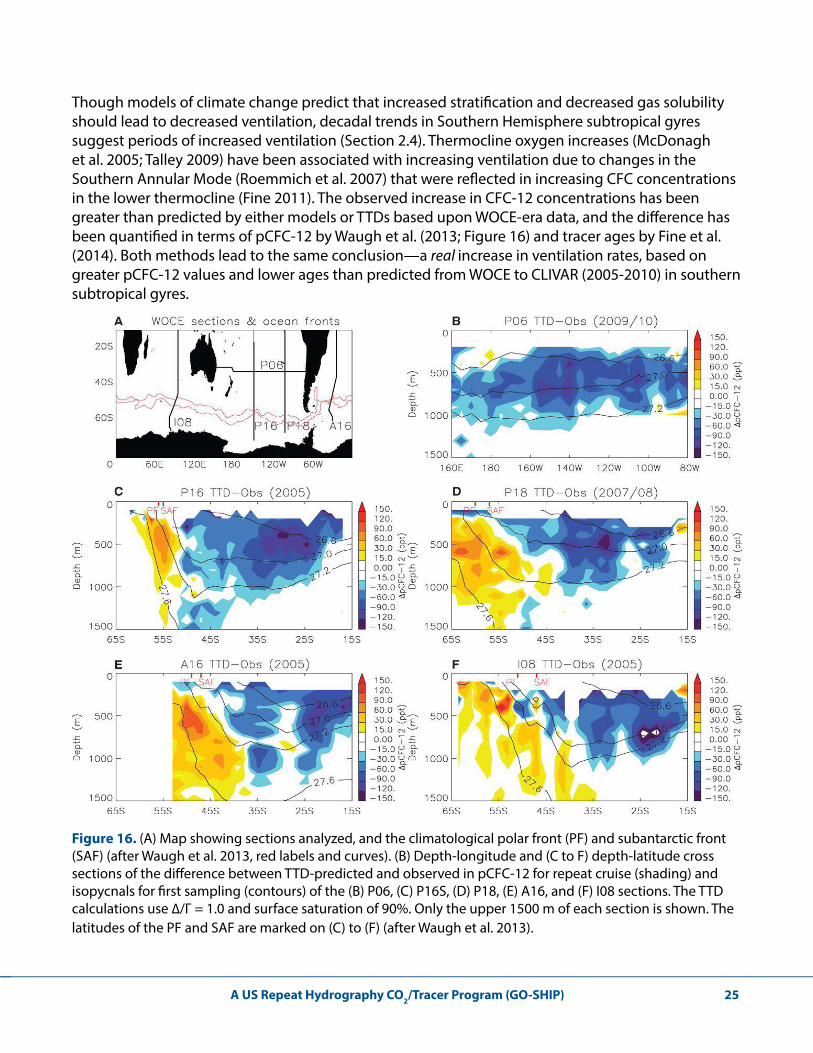
Though models of climate change predict that increased stratification and decreased gas solubility should lead to decreased ventilation, decadal trends in Southern Hemisphere subtropical gyres suggest periods of increased ventilation (Section 2.4). Thermocline oxygen increases (McDonagh et al. 2005; Talley 2009) have been associated with increasing ventilation due to changes in the Southern Annular Mode (Roemmich et al. 2007) that were reflected in increasing CFC concentrations in the lower thermocline (Fine 2011). The observed increase in CFC-12 concentrations has been greater than predicted by either models or TTDs based upon WOCE-era data, and the difference has been quantified in terms of pCFC-12 by Waugh et al. (2013; Figure 16) and tracer ages by Fine et al. (2014). Both methods lead to the same conclusion—a real increase in ventilation rates, based on greater pCFC-12 values and lower ages than predicted from WOCE to CLIVAR (2005-2010) in southern subtropical gyres.

Figure 16. (A) Map showing sections analyzed, and the climatological polar front (PF) and subantarctic front (SAF) (after Waugh et al. 2013, red labels and curves). (B) Depth-longitude and (C to F) depth-latitude cross sections of the difference between TTD-predicted and observed in pCFC-12 for repeat cruise (shading) and isopycnals for first sampling (contours) of the (B) P06, (C) P16S, (D) P18, (E) A16, and (F) I08 sections. The TTD calculations use ∆/Γ = 1.0 and surface saturation of 90%. Only the upper 1500 m of each section is shown. The latitudes of the PF and SAF are marked on (C) to (F) (after Waugh et al. 2013).


Transient tracer inventory calculations (Orsi et al. 1999, 2002; Smethie and Fine 2001; Rhein et al. 2002; LeBel et al. 2008; Smethie et al. 2007) provide integral water mass formation rates for deepwater masses where the time scale of ventilation is much greater than the decadal time scale for input of the tracer (Hall et al. 2007). As an example, North Atlantic CFC-12 inventory changes have shown a shift in the type of Labrador Sea Water (LSW) formed over the period 1997-2005. Classical LSW formation decreased (Rhein et al. 2011) while upper LSW formation increased (Kieke et al. 2006, 2007). Decreased classical LSW formation was accompanied by a decrease in subpolar gyre transport index (Curry and McCartney 2001; Kieke et al. 2007; Rhein et al. 2011) and a decrease in strength of the subpolar gyre from altimeter analysis (Hakkinen and Rhines 2004; Hakkinen et al. 2008).

Basin-wide CFC distributions highlight pathways of recently ventilated waters from the source regions. Recent float observations show the transport of LSW from the subpolar gyre into the subtropics by interior pathways, including on the western flank of the Mid-Atlantic Ridge (Bower and von Appen 2008, Bower et al. 2009). Although it is clear from the elevated concentrations of CFCs that the deep western boundary current is an important pathway into the subtropics, interior CFC concentrations support the importance also of interior pathways that are related to the role of eddies and winds (Lozier 2010).

2.6 Nutrients

Human impacts and shifting physical processes are altering the supply of nutrients to the ocean, and thereby exerting a control on the magnitude and variability of the ocean carbon biological pump (Doney 2010). Resampling of select WOCE sections during GO-SHIP (CLIVAR) are key for identifying trends and variability in nutrient content, for calibration of new-generation Argo nitrate sensors, and for application of nutrient-based ocean tracers to help elucidate physical and biogeochemical processes. For example, the large-scale warming of the surface ocean appears to be increasing stratification, thereby decreasing ventilation and the vertical flux of nutrients and, in low latitudes, reducing primary production. Kamykowski and Zentara (2005) estimated global ocean trends in nitrate availability to the pelagic through the 20th century and found that nitrate supply generally decreased during warming periods. Their results indicated that global surface water nitrate supply was lower in the last several decades than at any other time in the past century. Consistent with rising sea surface temperature and reduced nutrient availability, oligotrophic gyres in four of the world's major oceans expanded at average rates of 0.8% to 4.3% year-1 from 1998 to 2006, and this growth outpaced model projections (Polovina et al. 2008). While model projections suggest that nitrate concentrations will decrease in the upper 200 m of the central basins, in the ocean's thermocline, nitrate and phosphate are expected to increase at rates of ~0.3–0.5 and ~0.02–0.03 µmol kg-1 decade-1 respectively, concomitant with deoxygenation.

New generation optical nitrate sensors (ISUS) are now being incorporated into Argo floats, and are capable of collecting ~250 vertical casts during a three and half year deployment. Widespread use of these sensors could help to resolve spatiotemporal trends in upper-ocean nitrate content. However, due to the poor accuracy of these instruments, these data cannot be used to study variability and trends in deep ocean biogeochemistry without calibration against high-quality (e.g., GO-SHIP) nutrient data.


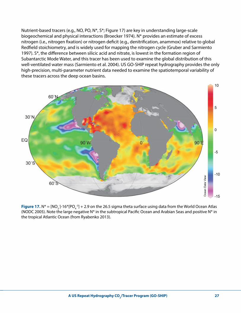
Nutrient-based tracers (e.g., NO, PO, N*, S*; Figure 17) are key in understanding large-scale biogeochemical and physical interactions (Broecker 1974). N* provides an estimate of excess nitrogen (i.e., nitrogen fixation) or nitrogen deficit (e.g., denitrification, anammox) relative to global Redfield stoichiometry, and is widely used for mapping the nitrogen cycle (Gruber and Sarmiento 1997). S*, the difference between silicic acid and nitrate, is lowest in the formation region of Subantarctic Mode Water, and this tracer has been used to examine the global distribution of this well-ventilated water mass (Sarmiento et al. 2004). US GO-SHIP repeat hydrography provides the only high-precision, multi-parameter nutrient data needed to examine the spatiotemporal variability of these tracers across the deep ocean basins.

Figure 17. N* = [NO3-]-16*[PO4

-3] + 2.9 on the 26.5 sigma theta surface using data from the World Ocean Atlas (NODC 2005). Note the large negative N* in the subtropical Pacific Ocean and Arabian Seas and positive N* in the tropical Atlantic Ocean (from Ryabenko 2013).


kuhlenbr

Typewritten Text



3 Structure of US GO-SHIP Repeat Hydrography

3.1 Relation to international GO-SHIP, WCRP, US CLIVAR, and OCB

US Repeat Hydrography, now known as US GO-SHIP, has been a major contributor to the international repeat hydrography observational network that has operated in the 2000s, with loosely organized contributions from numerous countries as a legacy of WOCE. By the time of the OceanObs09 meeting in 2009, it was clear that tighter international organization, including uniform data standards and reporting protocols, would be highly beneficial (Hood et al. 2010). The international GO-SHIP program was organized at that time. Strong, immediate benefits were regularizing communications between the involved countries, revision of WOCE data collection manuals, and the beginnings of a comprehensive international data policy, modeled on the US Repeat Hydrography data policy that has been functioning since 2003. With funding (Australia/Japan) of a program manager (M. Kramp) within JCOMM, and inclusion of GO-SHIP as a component of the Global Ocean Observing System, the next decade of GO-SHIP repeat hydrography will see well-coordinated collaborations and data management. The International Ocean Carbon Coordination Project (IOCCP) (http://www.ioccp.org) coordinates international ocean carbon efforts, while the SOLAS/IMBER Surface Interior Carbon (SIC) group provides scientific guidance and organizes global synthesis activities.

The US Repeat Hydrography Program receives funding from the NSF and NOAA, and has been tightly organized from the outset. The US program serves as a critical observational resource for and receives scientific and logistical support from members of the US CLIVAR (http://usclivar.org/) and the US Ocean Carbon and Biogeochemistry Program (http://www.us-ocb.org/) communities. The website http://ushydro.ucsd.edu contains thorough information about the organizational structure, data policies, and history of the program.

The US Repeat Hydrography Oversight Committee (RHOC), consisting of a subset of program principal investigators plus members of the community at large, plans and executes its ambitious program. The RHOC makes recommendations on changes in lines, sequencing, measurements, measurement teams, and entrainment of new scientists. They ensure smooth interactions with funding agencies and individual investigators (Level 3), and that adequate support is provided for data management. They serve as contact for coordinating with international GO-SHIP and IOCCP, and coordinate with the US CLIVAR and OCB steering committees. For each cruise, the RHOC selects a chief scientist, co-chief scientist, and up to five graduate or postdoctoral assistants through community-wide solicitations. They advocate adequate and consistent coverage of all Level 1 and 2 observations. With the evolution of the international GO-SHIP program, and evolution of US CLIVAR priorities toward sustained observations, the RHOC will evolve over the next several years, with tighter relationship to these overarching committees, membership rotation, and evolution of terms of reference.

http://www.ioccp.org

http://usclivar.org

http://www.us-ocb.org



The observing teams are highly experienced and routinely meet the highest standards necessary. The strict data policy is grounded on the assumption that the data are a shared community resource and should be publicly available as soon as possible. As we move forward via the proposed work to complete a second repeat cycle since WOCE, US CLIVAR has been evolving to include emphasis on sustained observations (http://www.usclivar.org/resources/observing-systems).

3.2 Data types

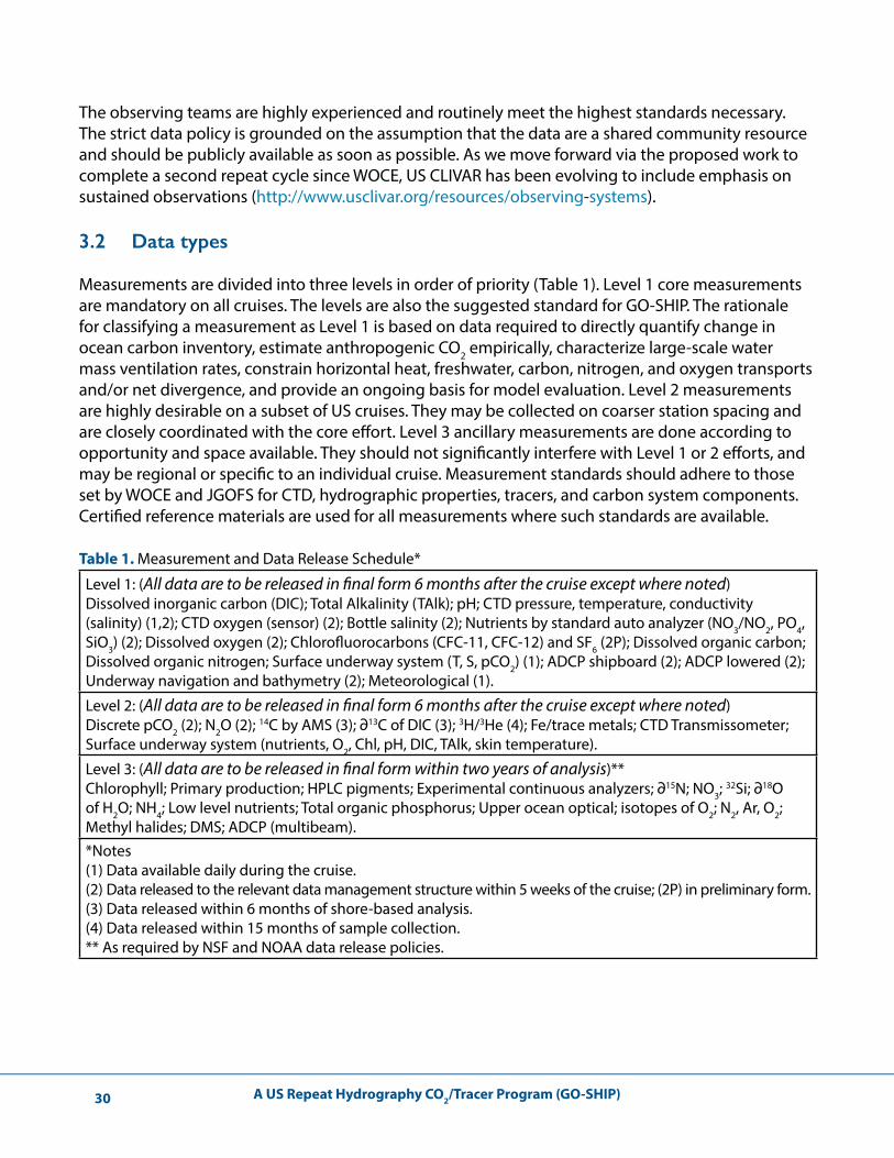
Measurements are divided into three levels in order of priority (Table 1). Level 1 core measurements are mandatory on all cruises. The levels are also the suggested standard for GO-SHIP. The rationale for classifying a measurement as Level 1 is based on data required to directly quantify change in ocean carbon inventory, estimate anthropogenic CO2 empirically, characterize large-scale water mass ventilation rates, constrain horizontal heat, freshwater, carbon, nitrogen, and oxygen transports and/or net divergence, and provide an ongoing basis for model evaluation. Level 2 measurements are highly desirable on a subset of US cruises. They may be collected on coarser station spacing and are closely coordinated with the core effort. Level 3 ancillary measurements are done according to opportunity and space available. They should not significantly interfere with Level 1 or 2 efforts, and may be regional or specific to an individual cruise. Measurement standards should adhere to those set by WOCE and JGOFS for CTD, hydrographic properties, tracers, and carbon system components. Certified reference materials are used for all measurements where such standards are available.

Table 1. Measurement and Data Release Schedule*

Level 1: (All data are to be released in final form 6 months after the cruise except where noted)Dissolved inorganic carbon (DIC); Total Alkalinity (TAlk); pH; CTD pressure, temperature, conductivity (salinity) (1,2); CTD oxygen (sensor) (2); Bottle salinity (2); Nutrients by standard auto analyzer (NO3/NO2, PO4, SiO3) (2); Dissolved oxygen (2); Chlorofluorocarbons (CFC-11, CFC-12) and SF6 (2P); Dissolved organic carbon; Dissolved organic nitrogen; Surface underway system (T, S, pCO2) (1); ADCP shipboard (2); ADCP lowered (2); Underway navigation and bathymetry (2); Meteorological (1).

Level 2: (All data are to be released in final form 6 months after the cruise except where noted) Discrete pCO2 (2); N2O (2); 14C by AMS (3); ∂13C of DIC (3); 3H/3He (4); Fe/trace metals; CTD Transmissometer; Surface underway system (nutrients, O2, Chl, pH, DIC, TAlk, skin temperature).

Level 3: (All data are to be released in final form within two years of analysis)** Chlorophyll; Primary production; HPLC pigments; Experimental continuous analyzers; ∂15N; NO3; 32Si; ∂18O of H2O; NH4; Low level nutrients; Total organic phosphorus; Upper ocean optical; isotopes of O2; N2, Ar, O2; Methyl halides; DMS; ADCP (multibeam).*Notes(1) Data available daily during the cruise.(2) Data released to the relevant data management structure within 5 weeks of the cruise; (2P) in preliminary form.(3) Data released within 6 months of shore-based analysis.(4) Data released within 15 months of sample collection.** As required by NSF and NOAA data release policies.

http://www.usclivar.org/resources/observing


3.3 Data policies

The US Repeat Hydrography data policy is stringent and geared toward rapid, open dissemination, with a clear structure for all data to undergo quality control, and to be sent to and available from recognized data centers. The policy includes: 1) All Level 1 and 2 observations, cruise reports, and metadata are made public in preliminary form through a specified data center soon after collection (“early release”), with final calibrated data provided six months after the cruise, with the exception of those data requiring on-shore analyses (see Table 1 and website); 2) All data collected as part of the program are submitted to a designated data management structure for quality control and dissemination for synthesis; and 3) A complete on-line cruise data inventory, applicable to all data collection programs, is posted within 60 days of the end of the cruise. All cruise data are tracked and linked to their data centers through the project's website http://ushydro.ucsd.edu. Ultimately, all US data are archived with the National Oceanographic Data Center (NODC) or other national data centers for some parameters, with the Level 1 and 2 data being archived well ahead of timelines set by the funding agencies.

3.4 Data track record and metrics

By all measures, the US Repeat Hydrography Program has consistently met virtually all targets for data collection and data reporting. Twenty-one cruises have been completed since the start of the US program in 2003; 13 were university-led and eight were NOAA-led. All cruises included a mixture of programs from NSF and NOAA. These were all of the cruises proposed for the first two cycles of funding since 2003, with one exception of cancellation of the Arabian Sea section I7N in 2009 for security reasons; resources were diverted to earlier completion of Pacific section P6, and the subsequent cruise schedule shifted. Any other minor adjustments of operations occurred because of ship equipment delays, which in a very few cases reduced the length of cruises, compensated for by slightly expanded station spacing.

The http://ushydro.ucsd.edu website, which is managed through the UCSD/SIO portion of the NSF funding for the program, tracks the submission of all US datasets, including all data types (Table 2). Success is greatly enhanced by the routine practice of contacting all principal investigators responsible for data submission approximately two months before each cruise, with a formal letter detailing the data center and timing required for data submission. US Repeat Hydrography Program provides regular post-cruise follow-up with every data originator. Data availability and access have been continually improving since the start of the program. The shipboard data management system and improved quality of analyses and quality control at sea have greatly improved data quality and decreased the effort to create the final datasets. Coordination between CCHDO and CDIAC (Table 2) in merging and quality control of datasets results in excellent availability and quality of the CTD and rosette sample profile data. Datasets at the other US Repeat Hydrography data centers (ADCP, LADCP, meteorology, bathymetry) are routinely updated and available soon after the cruises.

Formal metrics for ocean observing are being developed through the Ocean Observations Panel for Climate (OOPC). The US Repeat Hydrography Program has not yet formalized its metrics along the lines of the evolving Framework for Ocean Observing (FOO), which measures the program components in terms of Inputs (requirements and planning), Processes (observations, deployment




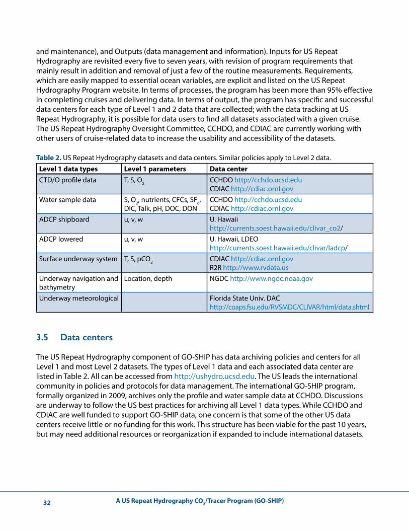
and maintenance), and Outputs (data management and information). Inputs for US Repeat Hydrography are revisited every five to seven years, with revision of program requirements that mainly result in addition and removal of just a few of the routine measurements. Requirements, which are easily mapped to essential ocean variables, are explicit and listed on the US Repeat Hydrography Program website. In terms of processes, the program has been more than 95% effective in completing cruises and delivering data. In terms of output, the program has specific and successful data centers for each type of Level 1 and 2 data that are collected; with the data tracking at US Repeat Hydrography, it is possible for data users to find all datasets associated with a given cruise. The US Repeat Hydrography Oversight Committee, CCHDO, and CDIAC are currently working with other users of cruise-related data to increase the usability and accessibility of the datasets.

Table 2. US Repeat Hydrography datasets and data centers. Similar policies apply to Level 2 data.

Level 1 data types Level 1 parameters Data centerCTD/O profile data T, S, O2 CCHDO http://cchdo.ucsd.edu

CDIAC http://cdiac.ornl.govWater sample data S, O2, nutrients, CFCs, SF6,

DIC, Talk, pH, DOC, DONCCHDO http://cchdo.ucsd.eduCDIAC http://cdiac.ornl.gov

ADCP shipboard u, v, w U. Hawaii http://currents.soest.hawaii.edu/clivar_co2/

ADCP lowered u, v, w U. Hawaii, LDEO http://currents.soest.hawaii.edu/clivar/ladcp/

Surface underway system T, S, pCO2 CDIAC http://cdiac.ornl.govR2R http://www.rvdata.us

Underway navigation and bathymetry

Location, depth NGDC http://www.ngdc.noaa.gov

Underway meteorological Florida State Univ. DAC http://coaps.fsu.edu/RVSMDC/CLIVAR/html/data.shtml

3.5 Data centers

The US Repeat Hydrography component of GO-SHIP has data archiving policies and centers for all Level 1 and most Level 2 datasets. The types of Level 1 data and each associated data center are listed in Table 2. All can be accessed from http://ushydro.ucsd.edu. The US leads the international community in policies and protocols for data management. The international GO-SHIP program, formally organized in 2009, archives only the profile and water sample data at CCHDO. Discussions are underway to follow the US best practices for archiving all Level 1 data types. While CCHDO and CDIAC are well funded to support GO-SHIP data, one concern is that some of the other US data centers receive little or no funding for this work. This structure has been viable for the past 10 years, but may need additional resources or reorganization if expanded to include international datasets.


http://cdiac.ornl.gov



http://currents.soest.hawaii.edu/clivar_co2

http://currents.soest.hawaii.edu/clivar/ladcp


http://www.rvdata.us

http://www.ngdc.noaa.gov

http://coaps.fsu.edu/RVSMDC/CLIVAR/html/data.shtml


GO-SHIP, including the large contribution from the US, builds on previous global-scale hydrography and re-occupations. The program evolves based on the findings of the previous

work. A major new focus of GO-SHIP is to determine trends and variability in marine biogeochemistry and ecosystems. These objectives will be incorporated into the sustained primary objectives of the US Repeat Hydrography Program under the auspices of GO-SHIP:

1. Reduce uncertainties in global freshwater, heat, and sea level budgets, especially in the otherwise data-sparse ocean below 2000 m;

2. Determine the distributions and controls of natural and anthropogenic carbon (both organic and inorganic);

3. Determine ocean ventilation and circulation pathways and rates using chemical tracers; 4. Determine the variability and controls in water mass properties and ventilation; 5. Determine the significance of a wide range of biogeochemically and ecologically important

properties on the carbon cycle in the ocean interior; and6. Test and validate new methodologies for conducting high-resolution physical and

biogeochemical measurements on autonomous vehicles.

These objectives are critical for evaluating and providing data constraints for state estimation, assimilation, and inverse models (e.g., Köhl et al. 2007; Macdonald et al. 2009; McDonagh et al. 2008; Lee et al. 2010; Heimbach et al. 2010; Wunsch and Heimbach 2013a, b, 2014). The ship-based hydrographic measurements will continue to provide a standard for validating new autonomous sensors and a reference/calibration dataset for other observing system elements (in particular Argo profiling floats and gliders). As biogeochemical sensors are added to these autonomous platforms, the repeat hydrography data will be invaluable for validating and calibrating these new sensors, and providing high-quality data for algorithm development of carbon system parameters from temperature salinity and oxygen data (Juranek et al. 2011). Hydrographic cruises also provide a means to access remote ocean areas for the deployment of these instruments.

The international hydrographic surveys of the 1990s (WOCE) and 2000s (CLIVAR Repeat Hydrography and GO-SHIP) were successful in answering many first-order questions about large-scale ocean circulation and carbon inventories. Their results also raised many new questions concerning ocean variability, circulation, and biogeochemical controls on carbon and tracer inventories, distributions, and long-term secular trends associated with climate change and ocean acidification. These observations showed that the ocean exhibits significant interannual variability on top of the expected smooth decadal trend as part of patterns of global change, complicating efforts to detect and attribute human influences on the ocean. WOCE and CLIVAR and other studies conducted over the last two decades show that the effect of climate forcing on the ocean is substantial, but not fully understood. The GO-SHIP hydrographic cruises need to be executed to examine the drivers and impacts of this variability, in concert with modeling and assimilation activities.

4 Future Science and Monitoring Objectives


The authors wish to thank the program managers of the National Science Foundation Division of Ocean Sciences and the National Oceanic and Atmospheric Administration Climate Program Office for their leadership and long-term support of the US Repeat Hydrography CO2/Tracer Program from its inception and into the future. The National Aeronautics and Space Administration has also been a long time supporter of the program’s biogeochemical and optical observations. We especially ex-press our heartfelt appreciation to all of the officers, crew, and scientists on the UNOLS and NOAA ships and in their laboratories, who operated the ships, stood on deck, worked with the instruments, and assembled these climate-quality datasets over the past 25 years. Their dedication has been truly exemplary. Finally, many thanks go to S. Bigley, K. Uhlenbrock, and H. Benway for their hours of effort preparing and editing this report.

Acknowledgments


References

Álvarez, M., T. Tanhua, H. Brix, C. Lo Monaco, N. Metzl, E. L. McDonagh, and H. L. Bryden, 2011: Decadal biogeochemical changes in the subtropical Indian Ocean associated with Subantarctic Mode Water. J. Geophys. Res.-Oceans, 116, C09016, doi: 10.1029/2010JC006475.

Azam, F., D. Smith, G. Steward, and A. Hagström, 1993: Bacteria-organic matter coupling and its significance for oceanic carbon cycling. Microb. Ecol., 28, 167–179, doi: 10.1007/BF00166806.

Bindoff, N. L., and T. J. McDougall, 2000: Decadal changes along an Indian Ocean section at 32°S and their interpretation. J. Phys. Oceanogr., 30, 1207–1222, doi: 10.1175/1520-0485(2000)030<1207:DCAAIO>2.0.CO;2.

Bindoff, N. L., et al., 2007: Observations: Oceanic climate change and sea level. Climate Change 2007: The Physical Science Basis. Contribution of Working Group I to the Fourth Assessment Report of the Intergovernmental Panel on Climate Change, S. Soloman, D. Qin, M. Manning, Z. Chen, M. Marquis, K. Averty, M. Tignor, and H. L. Miller, Eds. Cambridge University Press, 385-432.

Bower, A. S., and W.-J. von Appen., 2008: Interannual variability in the pathways of the North Atlantic Current over the Mid-Atlantic Ridge and the impact of topography. J. Phys. Oceanogr., 38, 104–120, doi: 10.1175/2007JPO3686.1.

Bower, A. S., M. S. Lozier, S. F. Gary, and C. W. Böning, 2009: Interior pathways of the North Atlantic meridional overturning circulation. Nature, 459, 243-247, doi:10.1038/nature07979.

Boyer, T. P., S. Levitus, J. I. Antonov, R. A. Locarnini, and H. E. Garcia, 2005: Linear trends in salinity for the World Ocean, 1955–1998. Geophys. Res. Lett., 32, L01604, doi: 10.1029/2004GL021791.

Broecker, W. S., 1974: “NO” A conservative water-mass tracer. Earth Planet. Sci. Lett., 23, 100–107, doi: 10.1016/0012-821X(74)90036-3.

Bryden, H. L., H. R. Longworth, and S. A. Cunningham, 2005: Slowing of the Atlantic meridional overturning circulation at 25°N. Nature, 438, 655–657, doi:10.1038/nature04385.

Bullister, J. L., 2014: Atmospheric CFC-11, CFC-12, CFC-113, CCl4, and SF6 histories (1910–2014), http://cdiac.ornl.gov/oceans/new_atmCFC.html.

Bullister, J. L., D. P. Wisegarver, and F. A. Menzia., 2002: The solubility of sulfur hexafluoride in water and seawater. Deep-Sea Res. I, 49, 175-187, doi: 10.1016/S0967-0637(01)00051-6.

Byrne, R. H., S. Mecking, R. A. Feely, and X. Liu, 2010: Direct observations of basin-wide acidification of the North Pacific. Geophys. Res. Lett., 37, L02601, doi:10.1029/2009GL040999.

Carlson, C. A., 2002: Production and removal processes. Biogeochemistry of Marine Dissolved Organic Matter, D. A. Hansell and C. A. Carlson, Eds., Academic Press, San Diego, 91–151.

http://dx.doi.org/10.1175/1520-0485(2000)030%3C1207:DCAAIO%3E2.0.CO;2

10.1038/nature

http://cdiac.ornl.gov/oceans/new_atmCFC.html

http://cdiac.ornl.gov/oceans/new_atmCFC.html


Carlson, C. A., H. W. Ducklow, and A. F. Michaels, 1994: Annual flux of dissolved organic carbon from the euphotic zone in the northwestern Sargasso Sea. Nature, 371, 405–408, doi:10.1038/371405a0.

Carlson, C. A., D. A. Hansell, N. B. Nelson, D. A. Siegel, W. M. Smethie, S. Khatiwala, M. M. Meyers, and E. Halewood, 2010: Dissolved organic carbon export and subsequent remineralization in the mesopelagic and bathypelagic realms of the North Atlantic basin. Deep-Sea Res. II, 57, 1433–1445.

Church, J. A., N. J. White, L. F. Konikow, C. M. Domingues, J. G. Cogley, E. Rignot, J. M. Gregory, M. R. van den Broeke, A. J. Monaghan, and I. Velicogna, 2011: Revisiting the Earth’s sea level and energy budgets from 1961 to 2008. Geophys. Res. Lett., 38, L18601, doi:10.1029/2001GL048794.

Clement, D., and N. Gruber, 2014: A C*-based extended multiple linear regression method to determine decadal changes in anthropogenic CO2 in the ocean. Abstract, 2014 Ocean Sciences Meeting, Honolulu, Hawaii.

Copin-Montgut, G., and B. Avril, 1993: Vertical distribution and temporal variation of dissolved organic carbon in the North-Western Mediterranean Sea. Deep-Sea Res. I, 40, 1963–1972, doi: 10.1016/0967-0637(93)90041-Z.

Currie, K. I., B. Gordon, S. Nichol, An. Gomez, R. Sparks, K. R. Lassey, and K. Riedel, 2011: Tropospheric 14CO2 at Wellington, New Zealand: The world’s longest record. Biogeochemistry, 104, 5–22, doi:10.1007/s10533-009-9352-6.

Curry, R. G., and M. S. McCartney, 2001: Ocean gyre circulation changes associated with the North Atlantic Oscillation. J. Phys. Oceanogr., 31, 3374–3400, doi: 10.1175/1520-0485(2001)0312.0.CO;2.

Deutsch, C., S. Emerson, and L. Thompson, 2005: Fingerprints of climate change in North Pacific oxygen. Geophys. Res. Lett., 32, L16604, doi: 10.1029/2005GL023190.

Dillon, T. M., 1982: Vertical overturns: A comparison of Thorpe and Ozmidov length scales. J. Geophys. Res., 87, 9601–9613, doi: 10.1029/JC087iC12p09601.

Doney, S. C., W. J. Jenkins, and J. L. Bullister, 1997: A comparison of ocean tracer dating techniques on a meridional section in the eastern North Atlantic. Deep-Sea Res. I, 44, 603–626, doi: 10.1016/S0967-0637(96)00105-7.

Doney, S. C., 2010: The growing human footprint on coastal and open-ocean biogeochemistry. Science, 328, 1512, doi:10.1126/science.1185198.

Durack, P. J., and S. E. Wijffels, 2010: Fifty-year trends in global ocean salinities and their relationship to broad-scale warming. J. Climate, 23, 4342–4362, doi:10.1175/2010jcli3377.1.

Durack, P. J., S. E. Wijffels, and R. J. Matear, 2012: Ocean salinities reveal strong global water cycle intensification during 1950 to 2000. Science, 336, 455–458, doi:10.1126/science.1212222.

Emerson, S., S. Mecking, and J. Abell, 2001: The biological pump in the subtropical North Pacific Ocean: Nutrient sources, Redfield ratios, and recent changes. Global Biogeochem. Cycles, 15, 535–554, doi: 10.1029/2000GB001320.

Emerson, S., Y. W. Watanabe, T. Ono, and S. Mecking, 2004: Temporal trends in apparent oxygen utilization in the upper pycnocline of the North Pacific: 1980–2000. J. Oceanogr., 60, 139–147, doi:10.1023/B:JOCE.0000038323.62130.a0.

10.1126/science

10.1126/science


Feely, R. A., C. L. Sabine, K. Lee, W. Berelson, J. Kleypas, V. J. Fabry, and F. J. Millero, 2004: Impact of anthropogenic CO2 on the CaCO3 system in the oceans. Science, 305, 362–366, doi:10.1126/science.1097329.

Feely, R. A., S. C. Doney, and S. R. Cooley, 2009: Ocean acidification: Present conditions and future changes in a high-CO2 world. Oceanography, 22, 36–47, doi:10.5670/oceanog.2009.95.

Ferron, B., H. Mercier, K. Speer, A. Gargett, and K. Polzin, 1998: Mixing in the Romanche Fracture Zone. J. Phys. Oceanogr., 28, 1929–1945, doi: 10.1175/1520-0485(1998)0282.0.CO;2.

Fine, R. A., 2011: Observations of CFCs and SF6 as ocean tracers. Annu. Rev. Mar. Sci., 3, 173–195, doi: 10.1146/annurev.marine.010908.163933.

Fine, R. A., S. Peacock, M. E. Maltrud, and F. O. Bryan, 2014: A new look at ocean ventilation timescales. Presentation, 2014 Ocean Sciences Meeting, Honolulu, Hawaii.

Frajka-Williams, E., S. A. Cunningham, H. Bryden, and B. A. King, 2011: Variability of Antarctic Bottom Water at 24.5°N in the Atlantic. J. Geophys. Res., 116, C11026, doi:10.1029/2011JC007168.

Friis, K., A. Körtzinger, J. Pätsch, and D. W. R. Wallace, 2005: On the temporal increase of anthropogenic CO2 in the subpolar North Atlantic. Deep-Sea Res. I, 52, 681–698, doi: 10.1016/j.dsr.2004.11.017.

Frölicher, T. L., F. Joos, G. K. Plattner, M. Steinacher, and S. C. Doney, 2009: Natural variability and anthropogenic trends in oceanic oxygen in a coupled carbon cycle-climate model ensemble. Global Biogeochem. Cycles, 23, GB1003, doi:10.1029/2008GB003316.

Ganachaud, A., and C. Wunsch, 2000: Improved estimates of global ocean circulation, heat transport and mixing from hydrographic data. Nature, 408, 453–456, doi:10.1038/35044048.

Gloor, M., N. Gruber, J. L. Sarmiento, C. L. Sabine, R. A. Feely, and C. Rödenbeck, 2003: A first estimate of present and preindustrial air-sea CO2 flux patterns based on ocean interior carbon measurements and models. Geophys. Res. Lett., 30, 1010, doi:10.1029/2002GL015594.

Goldberg, S., C. A. Carlson, B. Brock, N. B. Nelson, and D. A. Siegel, 2010: Meridional variability in dissolved organic matter stocks and diagenetic state within the euphotic and mesopelagic zone of the North Atlantic subtropical gyre. Mar. Chem., 56, 9–21., doi: 10.1016/j.marchem.2009.12.002.

Goldberg, S., C. Carlson, M. Brzezinski, N. Nelson, and D. Siegel, 2011: Systematic removal of neutral sugars within dissolved organic matter across ocean basins. Geophys. Res. Lett., 38, doi:10.1029/2011GL048620.

Gregg, M. C., 1989: Scaling turbulent dissipation in the thermocline. J. Geophys. Res., 94, 9686–9698, doi:10.1029/JC094iC07p09686.

Gruber, N., and J. L. Sarmiento, 1997: Global patterns of marine nitrogen fixation and denitrification. Global Biogeochem. Cycles, 11, 235–266 doi: 10.1029/97GB00077.

Gruber, N., J. L. Sarmiento, and T. F. Stocker, 1996: An improved method for detecting anthropogenic CO2 in the oceans. Global Biogeochem. Cycles, 10, 809–837, doi: 10.1029/96GB01608.

Gruber, N., M. Gloor, S. E. Mikaloff Fletcher, S. C. Doney, S. Dutkiewicz, M. J. Follows, M. Gerber, A. R. Jacobson, F. Joos, K. Lindsay, D. Menemenlis, A. Mouchet, S. A. Muller, J. L. Sarmiento, and T. Takahashi, 2009: Oceanic sources, sinks, and transport of atmospheric CO2. Global Biogeochem. Cycles, 23, GB1005, doi: 10.1029/2008GB003349.

http://www.pmel.noaa.gov/publications/search_abstract.php?fmContributionNum=2633


10.1126/science

10.1126/science




http://dx.doi.org/10.1029/JC094iC07p09686


Gruber, N., et al., 2014: The oceanic sink for anthropogenic CO2 since the mid-1990s. Abstract, 2014 Ocean Sciences Meeting, Honolulu, Hawaii.

Hakkinen, S., and P. B. Rhines, 2004: Decline of subpolar North Atlantic circulation during the 1990s. Science, 302, 555–55, doi: 10.1126/science.1094917.

Hakkinen, S., H. Hatun, and P. B. Rhines, 2008: Satellite evidence of change in the northern gyre. Arctic-Subarctic Ocean Fluxes: Defining the Role of the Northern Seas in Climate, B. Dickson, J. Meincke, and P. Rhines, Eds., Springer, 551–567.

Hall, T. M., T. W. N. Haine, M. Holzer, D. A. LeBel, F. Terenzi, and D. W. Waugh, 2007: Ventilation rates estimated from tracers in the presence of mixing. J. Phys. Oceanogr., 37, 2599–2611, doi: 10.1175/2006JPO3471.1.

Hansell, D. A., 2013: Recalcitrant dissolved organic carbon fractions. Annu. Rev. Mar. Sci., 5, 421-445, doi: 10.1146/annurev-marine-120710-100757.

Hansell, D. A., and C. A. Carlson, 1998: Net community production of dissolved organic carbon. Global Biogeochem. Cycles, 12, 443–453, doi: 10.1029/98GB01928.

Hansell, D. A., C. A. Carlson, D. J. Repeta, and R. Shlitzer, 2009. Dissolved organic matter in the ocean: A controversy stimulates new insights. Oceanography, 22, 202–211, doi: 10.5670/oceanog.2009.109.

Hansell, D. A., C. A. Carlson, and R. Schlitzer, 2012: Net removal of major marine dissolved organic carbon fractions in the subsurface ocean. Global Biogeochem. Cycles, 26, doi:10.1029/2011GB004069.

Hartin, C. A., R. A. Fine, I. Kamenkovich, and B. M. Sloyan, 2014: Comparison of Subantarctic Mode Water and Antarctic Intermediate Water formation rates in the South Pacific between NCAR-CCSM4 and observations. Geophys. Res. Lett., 41, 519–526, doi:10.1002/2013GL058728.

Heimbach, P., G. Forget, R. M. Ponte, C. Wunsch, M. Balmaseda, T. Awaji, J. Baehr, D. Behringer, J. Carton, N. Ferry, A. Fishcer, I. Fukumori, B. Geise, K. Haines, E. Harrison, F. Hernandez, M. Kamachi, C. Keppenne, A. Kohl, T. Lee, D. Menemenlis, P. Oke, E. Remy, M. Rienecker, A. Rosati, D. Smith, K. Speer, D. Stammer, and A. Weaver, 2010: Observational requirements for global-scale ocean climate analysis: Lessons from ocean state estimation, Proceedings of OceanObs’09: Sustained Ocean Observations and Information for Society (Vol. 2). 2009, J. Hall, D. E. Harrison, and D. Stammer, Eds., Venice, Italy, ESA Publication WPP-306, doi:10.5270/OceanObs09.cwp.42.

Helm, K. P., N. L. Bindoff, and J. A. Church, 2010: Changes in the global hydrological-cycle inferred from ocean salinity. Geophys. Res. Lett., 37. doi:10.1029/2010gl044222.

Helm, K. P., N. L. Bindoff, and J. A. Church, 2011: Observed decreases in oxygen content of the global ocean. Geophys. Res. Lett., 38, L23602, doi:10.1029/2011GL049513.

Hernández-Guerra, A., T. M. Joyce, E. Fraile-Nuez, and P. Vélez-Belchi, 2010: Using Argo data to investigate the meridional overturning circulation in the North Atlantic. Deep-Sea Res. I, 57, 29–36, doi: 10.1016/j.dsr.2009.10.003.

Hernández-Guerra, A., and L. D. Talley, 2014: Meridional overturning transports at 30°S in the Indian and Pacific oceans in 2002–2003 and 2009, in preparation.

10.5270/OceanObs09.cwp


Hood, M., M. Fukasawa, N. Gruber, G. C. Johnson, A. Körtzinger, C. Savine, B. Sloyan, K. Stansfield, and T. Tanhua, 2010: Ship-based repeat hydrography: A strategy for a sustained global program. Proceedings of OceanObs’09: Sustained Ocean Observations and Information for Society (Vol. 2). 2009, J. Hall, D. E. Harrison, and D. Stammer, Eds., Venice, Italy, ESA Publication WPP-306, doi: 10.5270/OceanObs09.cwp.42.

Huhn, O., M. Rhein, M. Hoppema, and S. van Heuven, 2013: Decline of deep and bottom water ventilation and slowing down of anthropogenic carbon storage in the Weddell Sea, 1984–2011. Deep Sea Res. I, 76, 66–84, doi: 10.1016/j.dsr.2013.01.005.

Huussen, T. N., A. C. Naveira-Garabato, H. L. Bryden, and E. L. McDonagh, 2012: Is the deep Indian Ocean MOC sustained by breaking internal waves? J. Geophys. Res., 117, C08024, doi:10.1029/2012JC008236.

IPCC, 2013: Climate Change 2013: The Physical Science Basis: Working Group I Contribution to the Fifth Assessment Report of the Intergovernmental Panel on Climate Change. T. F. Stocker, D. Qin, G.-K. Plattner, M. Tignor, S. K. Allen, J. Boschung, A. Nauels, Y. Xia, V. Bex and P. M. Midgley, Eds., Cambridge University Press, 1535 pp.

Jenkins, W. J., K. L. Elder, A. P. McNichol, and K. von Reden, 2010: The passage of the bomb radiocarbon pulse into the Pacific Ocean. Radiocarbon, 52, 1182–1190.

Johnson, G. C., 2008: Quantifying Antarctic Bottom Water and North Atlantic deep water volumes. J. Geophys. Res., 113, C05027, doi:10.1029/2007JC004477.

Johnson, G. C., and N. Gruber, 2007: Decadal water mass variations along 20°W in the northeastern Atlantic Ocean. Prog. Oceanogr., 73, 277–295, doi:10.1016/j.pocean.2006.03.022.

Johnson, G. C., and J. M. Lyman, 2007: Global oceans: Sea surface salinity. State of the Climate in 2006. A. Arguez,, Ed., Bull. Amer. Meteorol. Soc., 88, 6, S34–S35.

Johnson, G. C., S. G. Purkey, and J. M. Toole, 2008: Reduced Antarctic meridional overturning circulation reaches the North Atlantic Ocean. Geophys. Res. Lett., 35, L22601, doi:10.1029/2008GL035619.

Juranek, L. W., R. A. Feely, and D. Gilbert, 2011: Real-time estimation of pH and aragonite saturation state from Argo profiling floats: Prospects for an autonomous carbon observing strategy. Geophys. Res. Lett., 38, L17603, doi:10.1029/2011GL048580.

Kaiser, K., and R. Benner, 2009: Biochemical composition and size distribution of organic matter at the Pacific and Atlantic time-series stations. Mar. Chem., 113, 63–77, doi: 10.1016/j.marchem.2008.12.004.

Kamykowski, D., and S. J. Zentara, 2005: Changes in world ocean nitrate availability through the 20th century. Deep-Sea Res. I, 52, 1719–1744, doi: 10.1016/j.dsr.2005.04.007.

Katsumata, K., and M. Fukasawa, 2011: Changes in meridional fluxes and water properties in the Southern Hemisphere subtropical oceans between 1992/1995 and 2003/2004. Prog. Oceanogr., 89, 61–91, doi: 10.1016/j.pocean.2010.12.008.

Keeling, R. F., A. Kortzinger, and N. Gruber, 2010: Ocean deoxygenation in a warming world. Annu. Rev. Mar. Sci., 2, 199–229, doi: 10.1146/annurev.marine.010908.163855.


10.1016/j.dsr

10.1016/j.pocean


Keeling, R. F., and A. C. Manning, 2014: Studies of recent changes in atmospheric O2 content. Treatise on Geochemistry, 2nd ed., Vol. 5, H. D. Holland, and K. K. Turekian, Eds., Elsevier, 385-404.

Key, R. M., A. Kozyr, C. L. Sabine, K. Lee, R. Wanninkhof, J. L. Bullister, R. A. Feely, F. J. Millero, C. Mordy, and T.-H. Peng, 2004: A global ocean carbon climatology: Results from Global Data Analysis Project (GLODAP). Global Biogeochem. Cycles, 19, GB4031, doi:10.1029/2004GB002247.

Khatiwala, S., F. Primeau, and T. Hall, 2009: Reconstruction of the history of anthropogenic CO2 concentrations in the ocean. Nature, 462, 346–349, doi:10.1038/nature08526.

Khatiwala, S., T. Tanhua, S. Mikaloff Fletcher, M. Gerber, S. C. Doney, H. D. Graven, N. Gruber, G. A. McKinley, A. Murata, A. F. Rios, C. L. Sabine, and J. L. Sarmiento, 2012: Global ocean storage of anthropogenic carbon. Biogeosciences, 10, 2169–2191, doi:10.5194/bgd-9-8931-2012.

Kieke, D., M. Rhein, L. Stramma, W. M. Smethie, D. A. LeBel, and W. Zenk, 2006: Changes in the CFC inventories and formation rates of Upper Labrador Sea Water, 1997–2001. J. Phys. Oceanogr., 36, 64–86, doi:10.1029/2066GL028959.

Kieke, D., M. Rhein, L. Stramma, W. M. Smethie, J. L. Bullister, and D. A. LeBel, 2007: Changes in the pool of Labrador Sea Water in the subpolar North Atlantic. Geophys. Res. Lett., 34, doi:10.1029/2006GL028959.

Kobayashi, T., K. Mizuno, and T. Suga, 2012: Long-term variations of surface and intermediate waters in the southern Indian Ocean along 32°S. J. Oceanography, 68, 243–265, doi:10.1007/s10872-011-0093-5.

Köhl, A., D. Stammer, and B. Cornuelle, 2007: Interannual to decadal changes in the ECCO Global Synthesis. J. Phys. Oceanogr., 37, 313–337, doi:10.1175/JPO3014.1.

Kouketsu, S., M. Fukasawa, I. Kaneko, T. Kawano, H. Uchida, T. Doi, M. Aoyama, and K. Murakami, 2009: Changes in water properties and transports along 24°N in the North Pacific between 1985 and 2005. J. Geophys. Res., 114, C01008, doi:10.1029/2008JC004778.

Kouketsu, S., T. Doi, T. Kawano, S. Masuda N. Sugiura, Y. Sasaki, T. Toyoda, H. Igarashi, Y. Kawai, K. Katsumata, H. Uchida, M. Fukasawa, and T. Awaji, 2011: Deep ocean heat content changes estimated from observation and reanalysis product and their influence on sea level change. J. Geophys. Res., 116, C03012, doi:10.1029/2010JC006464.

Kunze, E., E. Firing, J. M. Hummon, T. K. Chereskin, and A. M. Thurnherr, 2006: Global abyssal mixing from lowered ADCP shear and CTD strain profiles. J. Phys. Oceanogr., 36, 1553–1576, doi:10.1175/JPO2926.1.

LeBel, D. A., W. M. Smethie, Jr., M. Rhein, D. Kieke, R. A. Fine, J. L. Bullister, D.-H. Min, W. Roether, R. F. Weiss, C. Andrie, D. Smythe-Wright, and E. P. Jones, 2008: The formation rate of North Atlantic Deep Water and Eighteen Degree Water calculated from CFC-11 inventories observed during WOCE. Deep-Sea Res. I, 55, 891–910, doi:10.1016/j.dsr.2008.03.009.

Lee, T., D. Stammer, T. Awaji. M. Balmaseda, D. Behringer, J. Carton, N. Ferry, A. Fishcer, I. Fukumori, B. Giese, K. Haines, E. Harrison, P. Heimbach, M. Kamachi, C. Keppenne, A. Köhl, S. Masina, D. Menemenlis, R. Ponte, E. Remy, M. Rienecker, A. Rosati, J. Schroester, D. Smith, A. Weaver, C. Wunsch, and Y. Xue, 2010: Ocean state estimation for climate research. Proceedings of OceanObs’09: Sustained Ocean Observations and Information for Society (Vol. 2). 2009, J. Hall, D. E. Harrison, and D. Stammer, Eds., Venice, Italy, ESA Publication WPP-306, doi:10.5270/OceanObs09.cwp.42.

10.1175/JPO



Lozier, M. S., 2010: Deconstructing the conveyor belt. Science, 328, 1507–1511, doi:10.1126/science.1189250.

Lumpkin, R., and K. Speer, 2007: Global ocean meridional overturning. J. Phys. Oceanogr., 37, 2550–2562, doi:10.1175/JPO3130.1.

Macdonald, A. M., S. Mecking, P. E. Robbins, J. M. Toole, G. C. Johnson, L. Talley, M. Cook, and S. E. Wijffels, 2009: The WOCE-Era 3-D Pacific Ocean circulation and heat budget. Prog. Oceanogr., 82, 281–325, doi:10.1016/j.pocean.2009.08.002

Masuda, S., T. Awaji, N. Sugiura, J. P. Matthews, T. Toyoda, Y. Kawai, T. Doi, S. Kouketsu, H. Igarashi, K. Katsumata, H. Uchida, T. Kawano, and M. Fukasawa, 2010: Simulated rapid warming of abyssal North Pacific water. Science, 329, 319–322, doi:10.1126/science.1188703.

Matear, R. J., and A. C. Hirst, 2003: Long-term changes in dissolved oxygen concentrations in the ocean caused by protracted global warming. Global Biogeochem. Cycles, 17, 1125, doi:10.1029/2002GB001997.

McDonagh, E. L., H. L. Bryden, B. A. King, R. J. Sanders, S. A. Cunningham, and R. Marsh, 2005: Decadal changes in the South Indian Ocean thermocline. J. Climate, 18, 1575–1590, doi:10.1175/JCLI3350.1.

McDonagh, E. L., H. L. Bryden, B. A. King, and R. J. Sanders, 2008: The circulation of the Indian Ocean at 32°S. Prog. Oceanogr., 79, 20–36, doi:10.1016/j.pocean.2008.07.001.

McNichol, A., R. M. Key, W. Jenkins, K. Elder, K. von Reden, A. Gagnon, and J. Burton, 2014: The WOCE/CLIVAR radiocarbon programs—Decadal changes in DI14C in the world’s oceans. Abstract, 2014 Ocean Sciences Meeting, Honolulu, Hawaii.

Mecking, S., G. C. Johnson, J. L. Bullister, and A. M. Macdonald, 2012: Decadal changes in oxygen and temperature-salinity relations along 32°S in the Indian Ocean through 2009. Abstract 2012 Ocean Sciences Meeting. Salt Lake City, Utah.

Mecking, S., C. Langdon, R. A. Feely, C. L. Sabine, C. A. Deutsch, and D.-H. Min, 2008: Climate variability in the North Pacific thermocline diagnosed from oxygen measurements: An update based on the US CLIVAR/CO2 Repeat Hydrography cruises. Global Biogeochem. Cycles, 22, GB3015, doi:10.1029/2007GB003101.

Mecking, S., M. J. Warner, and J. L. Bullister. 2006. Temporal changes in pCFC ages and AOU along two hydrographic sections in the eastern subtropical North Pacific. Deep-Sea Res. I, 53, 169–187, doi: 10.1016/j.dsr.2005.06.018.

Melet, A., R. Hallberg, S. Legg, and K. Polzin, 2013: Sensitivity of the Pacific Ocean state to the vertical distribution of internal-tide driven mixing. J. Phys. Oceanogr., 43, 602–615, doi:10.1175/JPO-D-12-055.1.

Moum, J., and J. Nash, 2009: Mixing measurements on an equatorial ocean mooring. J. Atmos. Ocean. Tech., 26, 317–336, doi:10.1175/2008JTECHO617.1.

Murata, A., Y. Kumamoto, S. Watanabe, and M. Fukasawa, 2007: Decadal increases of anthropogenic CO2 in the South Pacific subtropical ocean along 32°S. J. Geophys. Res., 112, C05033, doi:10.1029/2005JC003405.

10.1126/science

10.1126/science

10.1016/j.pocean

10.1126/science


Murata, A., Y. Kumamoto, K. Sasaki, S. Watanabe, and M. Fukasawa, 2010: Decadal increases in anthropogenic CO2 along 20°S in the South Indian Ocean. J. Geophys. Res., 115, C12055, doi:10.1029/2010JC006250.

Nash, J. D., J. N. Moum, and J. A. Mackinnon, 2014: Direct quantification of the large-scale distribution of mixing using temperature variance from shipboard CTD. Abstract, 2014 Ocean Sciences Meeting, Honolulu, Hawaii.

Naveira Garabato, A. C., K. L. Polzin, B. A. King, K. J. Heywood, and M. Visbeck, 2004: Widespread intense turbulent mixing in the Southern Ocean. Science, 303, 210–213, doi:10.1126/science.1090929.

NODC, 2005: World Ocean Atlas 2005 (WOA05). NOAA National Oceanographic Data Center, http://www.nodc.noaa.gov/OC5/WOA05/pr_woa05.html.

Olsen, A., R. M. Key, S. K. Lauvset, X. Lin, T. Tanhua, M. Hoppema, S. Jutterström, R. Steinfeldt, E. Jeansson, S. van Heuven, M. Ishii, T. Suzuki, A. Velo, A. Kozyr, and B. Pfeil, 2014: Global Ocean Data Analysis Project Version 2 (GLODAPv2), 2014 Ocean Sciences Meeting, Honolulu, Hawaii.

Orr, J. C., V. J. Fabry, O. Aumont, L. Bopp, S. C. Doney, R. A. Feely, A. Gnanadesikan, N. Gruber, A. Ishida F. Joos R. M. Key, K. Lindsay, E. Maier-Reimer, R. Matear, P. Monfray, A. Mouchet, R. G. Najjar, G.-K. Plattner, K. B. Rodgers, C. L. Savine, J. L. Sarmiento, R. Schlitzer, R. D. Slater, I. J. Totterdell, M. F. Weirig, Y. Yamanaka, and A. Yool, 2005: Anthropogenic ocean acidification over the twenty-first century and its impact on calcifying organisms. Nature, 437, 681–686, doi:10.1038/nature04095.

Orsi, A. H., G. C. Johnson, and J. L. Bullister, 1999: Circulation, mixing and production of Antarctic Bottom Water. Prog. Oceanogr., 43, 55–109, doi:10.1016/S0079-6611(99)00004-X.

Orsi, A. H., W. M. Smethie, Jr., and J. L. Bullister, 2002: On the total input of Antarctic waters to the deep ocean: A preliminary estimate from chlorofluorocarbon measurements. J. Geophys. Res., 107, 31-1–31-14., doi:10.1029/2001JC000976.

Orsi, A. H., and T. Whitworth, III, 2005: Hydrographic Atlas of the World Ocean Circulation Experiment (WOCE), Vol. 1, Southern Ocean. M. Sparrow, P. Chapman, and J. Gould Eds., Int. WOCE Project Office, Southampton, UK, http://woceatlas.tamu.edu/.

Otto, A., F. E. L. Otto, O. Boucher, J. Church, G. Hegerl, P. M. Forster, N. P. Gillett, J. Gregory, G. C. Johnson, R. Knutti, N. Lewis, U. Lohmann, J. Marotzke, G. Myhre, D. Shindell, B. Stevens, and M. R. Allen, 2013: Energy budget constraints on climate response. Nat. Geosci., 6, 415-416, doi:10.1038/ngeo1836.

Owens, W. B., and A. P. S. Wong, 2009: An improved calibration method for the drift of the conductivity sensor on autonomous CTD profiling floats by theta-S climatology. Deep-Sea Res. I, 56, 450–457, doi:10.1016/j.dsr.2008.09.008.

Palmer, M. D., H. L. Bryden, J. Hirschi, and J. Marotzke, 2004: Observed changes in the South Indian Ocean gyre circulation, 1987-2002. Geophys. Res. Lett., 31, L15303, doi:10.1029/2004GL020506.

Palmer, M. D., A. C. Naveira Garabato, J. D. Stark, J. J.-M. Hirschi, and J. Marotzke, 2007: The influence of diapycnal mixing on quasi-steady overturning states in the Indian Ocean. J. Phys. Oceanogr., 37, 2290–2304, doi:10.1175/JPO3117.1.

www.nodc.noaa.gov/OC5/WOA05/pr_woa05.html

http://woceatlas.tamu.edu/

10.1038/ngeo

10.1038/ngeo

10.1016/j.dsr


Pardo, P. C., F. F. Pérez, S. Khatiwala, and A. F. Ríos, 2014: Anthropogenic CO2 estimates in the Southern Ocean: Storage partitioning in the different water masses. Prog. Oceanogr., 120, 230–242, doi: 10.1016/j.pocean.2013.09.005.

Peacock, S., M. Maltrud, and R. Bleck, 2005: Putting models to the data test: A case study using Indian Ocean CFC-11 data. Ocean Model., 9, 1-22, doi:10.1016/j.ocemod.2004.02.004.

Pérez , F. F., M. Vázquez-Rodríguez, H. Mercier, A. Velo, P. Lherminier, and A. F. Ríos, 2010: Trends of anthropogenic CO2 storage in North Atlantic water masses. Biogeosciences, 7, 1789–1807, doi:10.5194/bg-7-1789-2010.

Pérez , F. F., H. Mercier, M. Vázquez-Rodríguez, P. Lherminier, A. Velo, P. C. Pardo, G. Roson, and A. F. Ríos, 2013: Atlantic Ocean CO2 uptake reduced by weakening of the meridional overturning circulation. Nat. Geosci., 6, 146–152, doi:10.1038/ngeo1680.

Perlin, A., and J. Moum, 2012: Comparison of thermal variance dissipation rates from moored and profiling instruments at the equator. J. Atmos. Ocean Tech., 29, 1347–1362, doi:10.1175/JTECH-D-12-00019.1.

Polovina, J. J., E. A. Howell, and M. Abecassis, 2008: Ocean’s least productive waters are expanding. Geophys. Res. Lett., 35, L03618, doi:10.1029/2007GL031745.

Polzin, K. L., J. M. Toole, and R. W. Schmitt, 1995: Finescale parameterizations of turbulent dissipation. J. Phys. Oceanogr., 25, 306–328, doi:10.1175/1520-0485(1995)025<0306:FPOTD>2.0.CO;2.

Polzin, K. L., A. C. N. Garabato, T. N. Huussen, B. M. Sloyan, and S. Waterman, 2014: Finescale parameterizations of turbulent dissipation. J. Geophys. Res. Oceans, 119, doi:10.1002/2013JC008979.

Purkey, S. G., and G. C. Johnson, 2010: Warming of global abyssal and deep Southern Ocean waters Between the 1990s and 2000s: Contributions to global heat and sea level rise budgets. J. Climate, 23, 6336–6351, doi:10.1175/2010JCLI3682.1.

Purkey, S. G., and G. C. Johnson, 2012: Global contraction of Antarctic Bottom Water between the 1980s and 2000s. J. Climate, 25, 5830–5844, doi:10.1175/JCLI-D-11-00612.1.

Purkey, S. G., and G. C. Johnson, 2013: Antarctic Bottom Water warming and freshening: Contributions to sea level rise, ocean freshwater budgets, and global heat gain. J. Climate, 26, doi:10.1175/JCLI-D-12-00834.1.

Reed, A., M. J. Warner, R. Sonnerup, J. L. Bullister, and S. Rintoul, 2014: Decreasing Antarctic Bottom Water production in the Australia-Antarctic Basin. J. Geophys. Res., submitted.

Reid, J. L., 2003: On the total geostrophic circulation of the Indian Ocean; Flow patterns, tracers and transports. Prog. Oceanogr., 56, 137–186, doi: 10.1016/S0079-6611(02)00141-6.

Rhein, M., J. Fischer, W. M. Smethie, Jr., D. Smythe-Wright, D. H. Min, C. Mertens, U. Fleischmann, A. Putzka, and R. F. Weiss, 2002: Labrador Sea Water: Pathways, CFC-inventory and formation rates. J. Phys. Oceanogr., 32, 648–665, doi: 10.1175/1520-0485(2002)032<0648:LSWPCI>2.0.CO;2.

Rhein, M., D. H. Kieke, S. Huttl-Kabus, A. Roessler, C. Mertens, R. Meissner, B. Klein, C. W. Boning, and I. Yashayaev, 2011: Deep water formation, the subpolar gyre, and the meridional overturning circulation in the subpolar North Atlantic. Deep-Sea Res. II, 58, 1819–1832, doi: 10.1016/j.dsr2.2010.10.061.

10.1038/ngeo

10.1175/JCLI

10.1175/JCLI

10.1175/JCLI


Rhein, M., S. R. Rintoul, S. Aoki, E. Campos, D. Chambers, R. A. Feely, S. Gulev, G. C. Johnson, S. A. Josey, A. Kostianoy, C. Mauritzen, D. Roemmich, L. D. Talley, and F. Wang, 2013: Observations: Ocean. Climate Change 2013: The Physical Science Basis. Contribution of Working Group I to the Fifth Assessment Report of the Intergovernmental Panel on Climate Change, T. F. Stocker, D. Qin, G.-K. Plattner, M. Tignor, S. K. Allen, J. Boschung, A. Nauels, Y. Xia, V. Bex, and P. M. Midgley, Eds., Cambridge University Press, 255-310.

Rignot, E., J. L. Bamber, M. R. van Den Broeke, C. Davis, Y. Li, W. Jan Van De Berg, and E. van Meijgaard, 2008: Recent Antarctic ice mass loss from radar interferometry and regional climate modeling. Nat. Geosci., 1, 106–110, doi:10.1038/ngeo102.

Rintoul, S. R., 2007: Rapid freshening of Antarctic Bottom Water formed in the Indian and Pacific oceans. Geophys. Res. Lett., 34, L06606, doi:10.1029/2006GL028550.

Robbins, P. E., and J. M. Toole, 1997: The dissolved silica budget as a constraint on the meridional overturning circulation in the Indian Ocean. Deep-Sea Res. I, 44, 879–906, doi:10.1016/S0967-0637(96)00126-4.

Roemmich. D., J. Gilson, R. Davis, P. Sutton, S. Wijffels, and S. Riser, 2007: Decadal spinup of the South Pacific subtropical gyre. J. Phys. Oceanogr., 37, 162–173, doi:10.1175/JPO3004.1.

Roemmich, D., and C. Wunsch, 1984: Apparent changes in the climate state of the deep North Atlantic Ocean. Nature, 307, 447–450, doi:10.1038/307447a0.

Ryabenko, E., 2013: Stable isotope methods for the study of the nitrogen cycle. Topics in Oceanogr., E. Zambianchi Ed., InTech, 1-40, doi:10.5772/56105.

Sabine, C. L., R. A. Feely, N. Gruber, R. M. Key, K. Lee, J. L. Bullister, R. Wanninkhof, C. S Wong, D. W. R. Wallace, B. Tilbrook, F. J. Millero, T.-H. Peng, A. Kozyr, T. Ono, and A. F. Rios, 2004: The oceanic sink for anthropogenic CO2. Science, 305, 367–371, doi:10.1126/science.1097403.

Sabine, C. L., R. A. Feely, F. J. Millero, A. G. Dickson, C. Langdon, S. Mecking, and D. Greeley, 2008: Decadal changes in Pacific carbon. J. Geophys. Res., 113, C07021, doi:10.1029/2007JC004577.

Sabine, C. L., and T. Tanhua, 2010: Estimation of anthropogenic CO2 inventories in the ocean. Annu. Rev. Mar. Sci., 2, 175–198, doi:10.1146/annurev-marine-120308-080947.

Sarmiento, J. L., N. Gruber, M. A. Brzezinski, and J. P. Dunne, 2004: High-latitude controls of thermocline nutrients and low latitude biological productivity. Nature, 427, 56–60, doi:10.1038/nature02127.

Sheen, K. L., J. A. Brearley, A. C. Naveira Garabato, D. A. Smeed, S. Waterman, J. R. Ledwell, M. P. Meredith, L. St. Laurent, A. M. Thurnherr, J. M. Toole, and A. J. Watson, 2013: Rates and mechanisms of turbulent dissipation and mixing in the Southern Ocean: Results from the Diapycnal and Isopycnal Mixing Experiment in the Southern Ocean (DIMES). J. Geophys. Res., 118, 2774–2779, doi:10.1002/jgrc.20217.

Skoog, A., and R. Benner, 1997: Aldoses in various size fractions of marine organic matter: Implications for carbon cycling. Limnol. Oceanogr., 42, 1803–1813.

Sloyan, B. M., 2005: Spatial variability of mixing in the Southern Ocean. Geophys. Res. Lett., 32, L18603, doi:10.1029/2005GL023568.

10.1038/ngeo



10.1126/science

10.1146/annurev


Sloyan, B. M., 2006: Antarctic bottom and lower circumpolar deep water circulation in the eastern Indian Ocean. J. Geophys. Res., 111, C02006, doi:10.1029/2005JC003011.

Sloyan, B., L. D. Talley, T. Chereskin, R. Fine, and J. Holte, 2010: Antarctic Intermediate water and Subantarctic Mode water formation in the southeast Pacific: The role of turbulent mixing. J. Phys. Oceanogr., 40, 1558-1574. doi:10.1175/2010JPO4114.1.

Sloyan, B. M., S. E. Wijffels, B. Tilbrook, K. Katsumata, A. Murata, and A. M. Macdonald, 2013: Deep ocean changes near the western boundary of the South Pacific Ocean. J. Phys. Oceanogr., 43, 2132–2141, doi:10.1175/JPO-D-12-0182.1.

Smethie, W. M., and R. A Fine, 2001: Rates of North Atlantic Deep Water formation calculated from chlorofluorocarbon inventories. Deep Sea Res. I, 48, 189–215, doi:10.1016/S0967-0637(00)00048-0.

Smethie, W. M., D. A. LeBel, R. A. Fine, M. Rhein, and D. Kieke. 2007: Strength and variability of the deep limb of the North Atlantic meridional overturning circulation from chlorofluorocarbon inventories. Past and Future Changes of the Ocean’s Meridional Overturning Circulation: Mechanisms and Impacts, A. Schmittner, J. Chiang, and S. Hemming, Eds., AGU Geophysical Monograph Series, 173, 119–130.

Sonnerup, R., S. Mecking, and J. Bullister, 2013: Transit time distributions and oxygen utilization rates in the northeast Pacific Ocean from chlorofluorocarbons and sulfur hexafluoride. Deep-Sea Res. I, 72, 61–71, doi:10.1016/j.dsr.2012.10.013.

Stramma, L., S. Schmidtko, L. A. Levin, and G. C. Johnson, 2010: Ocean oxygen minima expansions and their biological impacts. Deep-Sea Res. I, 57, 587–595, doi:10.1016/j.dsr.2010.01.005.

Stramma, L., A. Oschlies, and S. Schmidtko, 2012: Mismatch between observed and modeled trends in dissolved upper-ocean oxygen over the last 50 yr. Biogeosciences, 9, 4045–4057, doi:10.5194/bg-9-4045-2012.

Swift, J. H., and A. H. Orsi, 2012: Sixty-four days of hydrography and storms: RVIB Nathaniel B. Palmer’s 2011 S04P Cruise. Oceanography, 25, 54–55, doi:10.5670/oceanog.2012.74.

Takahashi, T., et al., 2009: Climatological mean and decadal change in surface ocean pCO2, and net sea-air CO2 flux over the global oceans. Deep-Sea Res. I, 56, 2075–2076, doi:10.1016/j.dsr2.2008.12.009.

Talley, L. D., 2007: Hydrographic Atlas of the World Ocean Circulation Experiment (WOCE), Vol. 2: Pacific Ocean. M. Sparrow, P. Chapman, and J. Gould, Eds., International WOCE Project Office, Southampton, UK, http://www-pord.ucsd.edu/whp_atlas/pacific_index.html.

Talley, L. D., 2009: Review of ocean temperature, salinity and oxygen changes in the Pacific and subtropical southern hemisphere. 2009 IOP Conference Series: Earth Environ. Sci.. 6, 032009, doi:10.1088/1755-1307/6/3/032009.

Talley, L. D., 2013: Hydrographic Atlas of the World Ocean Circulation Experiment (WOCE), Vol. 4, Indian Ocean, M. Sparrow, P. Chapman, and J. Gould, Eds., International WOCE Project Office, Southampton, UK, http://www-pord.ucsd.edu/whp_atlas/indian_index.html.

Tanhua, T., D. W. Waugh, and J. L. Bullister, 2013: Estimating changes in ocean ventilation from early 1990s CFC-12 and late 2000s SF6 measurements. Geophys. Res. Lett., 40, 927–932, doi:10.1002/grl.50251.

10.1175/JPO

10.5670/oceanog

http://www-pord.ucsd.edu/whp_atlas/pacific_index.html

http://www-pord.ucsd.edu/whp_atlas/indian_index.html

10.1002/grl

10.1002/grl


Tanhua, T., D. W. Waugh, and D. W. R. Wallace, 2008: Use of SF6 to estimate anthropogenic CO2 in the upper ocean. J. Geophys. Res., 113, doi:10.1029/2007JC004416.

Thurnherr, A. M., 2011: Vertical velocity from LADCP data. Proceeding, CWTMC’11 IEEE, Monterey, California.

Thurnherr, A. M., L. C. St. Laurent, K. J. Richards, and J. M. Toole, 2014: A universal vertical-wavenumber spectrum of high-frequency internal waves in the ocean, in preparation.

van Heuven, S. M. A. C., M. Hoppema, O. Huhn, H. A. Slagter, H. J. W. de Baar, 2011: Direct observation of increasing CO2 in the Weddell Gyre along the Prime Meridian during 1973–2008. Deep-Sea Res. II, 58, 2613–2635, doi:10.1016/j.dsr2.2011.08.007.

Walker, S. J., R. F. Weiss, and P. K. Salameh, 2000: Reconstructed histories of the annual mean atmospheric mole fractions for the halocarbons CFC-11, CFC-12, CFC-113, and carbon tetrachloride. J. Geophys. Res., 105, 14,285–14,296, doi:10.1029/1999JC900273.

Wanninkhof, R., S. C. Doney, J. L. Bullister, N. M. Levine, M. Warner, and N. Gruber, 2010: Detecting anthropogenic CO2 changes in the interior Atlantic Ocean between 1989 and 2005. J. Geophys. Res., 115, C11028, doi:10.1029/2010JC006251.

Wanninkhof, R., G.-H. Park, T. Takahashi, R. A. Feely, J. L. Bullister, and S. C. Doney, 2013a: Changes in deep-water CO2 concentrations over the last several decades determined from discrete pCO2 measurements. Deep-Sea Res. I., 74, 48–63, doi:10.1016/j.dsr.2012.12.005.

Wanninkhof, R., G.-H. Park, T. Takahashi, C. Sweeney, R. Feely, Y. Nojiri, N. Gruber, S. C. Doney, G. A. McKinley, A. Lenton, C. Le Quéré, C. Heinze, J. Schwinger, H. Graven, and S. Khatiwala, 2013b: Global ocean carbon uptake: Magnitude, variability and trends. Biogeosciences, 10, 1983–2000, doi:10.5194/bg-10-1983-2013.

Warner, M. J., and R. F. Weiss, 1985: Solubilities of chlorofluorocarbons 11 and 12 in water and seawater. Deep-Sea Res., 32, 1485–1497, doi: 0.1016/0198-0149(85)90099-8.

Waterhouse, A., J. A. MacKinnon, J. D. Nash, M. H. Alford, E. Kunze, H. L. Simmons, K. L. Polzin, L. C. St. Laurent, O. M. Sun, R. Pinkel, L. D. Talley, C. B. Whalen, T. N. Huuseen, C. G. Carter, I. Fer, S. Waterman, A. C. Naveira Garabato, T. B. Sanford, And C. M. Lee, 2014: Global patterns of diapycnal mixing from measurements of the turbulent dissipation rate. J. Phys. Oceanogr., 44, 1854-1872, doi:10.1175/JPO-D-13-0104.1.

Waterman, S., A. C. Naveira Garabato, and K. L. Polzin, 2013: Internal waves and turbulence in the Antarctic Circumpolar Current. J. Phys. Oceanogr., 43, 259–282, doi: 10.1175/JPO-D-11-0194.1.

Waugh, D. W., T. M. Hall, and T. W. N. Haine, 2003: Relationships among tracer ages. J. Geophys. Res., 108, doi:10.1029/2002JC001325.

Waugh, D. W., F. Primeau, T. Devries, and M. Holzer, 2013: Recent changes in the ventilation of the Southern Oceans. Science, 339, 568–570, doi:10.1126/science.1225411.

Whalen, C. B., L. D. Talley, and J. A. MacKinnon, 2012: Spatial and temporal variability of global ocean mixing inferred from Argo profiles. Geophys. Res. Lett., 39, L18612, doi:10.1029/2012GL053196.

10.1016/j.dsr

10.1016/j.dsr

10.1126/science


Whitney, F. A., H. J. Freeland, and M. Robert, 2007: Persistently declining oxygen levels in the interior waters of the eastern subarctic Pacific. Prog. Oceanogr., 75, 179–199, doi:10.1016/j.pocean.2007.08.007.

Wunsch, C., and P. Heimbach, 2013a: Dynamically and kinematically consistent global ocean circulation and ice state estimates. Ocean Circulation and Climate: A 21st Century Perspective. G. Siedler, J. Church, J. Gould, and S. Griffies, Eds., Elsevier, 553–579, doi:10.1016/B978-0-12-391851-2.00021-0.

Wunsch, C., and P. Heimbach, 2013b: Two decades of the Atlantic meridional overturning circulation: Anatomy, variations, extremes, prediction, and overcoming its limitations. J. Climate, 26, 7167–7186, doi:10.1175/JCLI-D-12-00478.1.

Wunsch, C., and P. Heimbach, 2014: Bidecadal thermal changes in the abyssal ocean. J. Phys. Oceanogr., doi:10.1175/JPO-D-13-096.1.

Yool, A., E. E. Popova, A. C. Coward, D. Bernie, and T.R. Anderson, 2013: Climate change and ocean acidification impacts of lower trophic levels and the export of organic carbon to the deep ocean. Biogeosciences, 10, 5831–5854, doi:10.5194/bg-10-5831-2013.

10.1175/JCLI

10.1175/JPO

10.5194/bg

US CLIVARClimate Variability & Predictabilit

y

US CLIVAR acknowledges support from these US agencies:

This material was developed with federal support of NASA (AGS-0963735), NOAA (NA11OAR4310213), NSF (AGS-0961146), and DOE (AGS-1357212).

Any opinions, findings, conclusions or recommendations expressed in this material are those of the authors and do not necessarily reflect the views of the sponsoring agencies.

U.S. DEPARTMENT OF COM

ME

RCE

NATIONAL

OCEA

NICAND

ATMOSPHERIC ADMINISTR

ATION

US Climate Variability & Predictability Program

1201 New York Ave NW, Suite 400Washington, D C 20005

(202) 787-1682www.usclivar.org

[email protected]/usclivar

OCB acknowledges support from these US agencies:

This material was developed with federal support of NASA (NNX14AD47G) and NSF (1233249).

Any opinions, findings, conclusions or recommendations expressed in this material are those of the authors and do not necessarily reflect the views of the sponsoring agencies.

Ocean Carbon & Biogeochemistry ProgramWoods Hole Oceanographic Institution

266 Woods Hole RoadWoods Hole, MA 02543

(508) 289-2838www.us-ocb.org

[email protected]

www.usclivar.org

mailto:[email protected]

twitter.com/usclivar

www.us-ocb.org

mailto:[email protected]

Documents

THE US REPEAT HYDROGRAPHY CO /TRACER … · ACCOMPLISHMENTS FROM THE FIRST DECADAL SURVEY ... /Tracer Program (GO-SHIP): Accomplishments from the first decadal ... /Tracer Program