The use of historical range and variability (HRV) in ... · Review The use of historical range and variability (HRV) in landscape management Robert E. Keane a,*, Paul F. Hessburg

Review

The use of historical range and variability (HRV) in landscape management

Robert E. Keane a,*, Paul F. Hessburg b,1, Peter B. Landres c, Fred J. Swanson d,2

a USDA Forest Service, Rocky Mountain Research Station, Missoula Fire Sciences Laboratory, 5775 Highway 10 West, Missoula, MT 59808, United Statesb USDA Forest Service, Pacific Northwest Research Station, Forestry Sciences Laboratory, 1133 North Western Avenue, Wenatchee, WA 98801, United Statesc USDA Forest Service, Rocky Mountain Research Station, Missoula Forestry Sciences Laboratory, Missoula, MT 59807, United Statesd USDA Forest Service, Pacific Northwest Research Station, Forestry Sciences Laboratory, 3200 SW Jefferson Way, Corvallis, OR 97331, WA, United States

Contents

1. Introduction . . . . . . . . . . . . . . . . . . . . . . . . . . . . . . . . . . . . . . . . . . . . . . . . . . . . . . . . . . . . . . . . . . . . . . . . . . . . . . . . . . . . . . . . . . . . . . . . . . . . 1026

1.1. Background . . . . . . . . . . . . . . . . . . . . . . . . . . . . . . . . . . . . . . . . . . . . . . . . . . . . . . . . . . . . . . . . . . . . . . . . . . . . . . . . . . . . . . . . . . . . . . . 1026

2. Quantifying HRV . . . . . . . . . . . . . . . . . . . . . . . . . . . . . . . . . . . . . . . . . . . . . . . . . . . . . . . . . . . . . . . . . . . . . . . . . . . . . . . . . . . . . . . . . . . . . . . . 1028

3. Applying HRV. . . . . . . . . . . . . . . . . . . . . . . . . . . . . . . . . . . . . . . . . . . . . . . . . . . . . . . . . . . . . . . . . . . . . . . . . . . . . . . . . . . . . . . . . . . . . . . . . . . 1030

4. Advantages of HRV . . . . . . . . . . . . . . . . . . . . . . . . . . . . . . . . . . . . . . . . . . . . . . . . . . . . . . . . . . . . . . . . . . . . . . . . . . . . . . . . . . . . . . . . . . . . . . 1030

5. Limitations of HRV. . . . . . . . . . . . . . . . . . . . . . . . . . . . . . . . . . . . . . . . . . . . . . . . . . . . . . . . . . . . . . . . . . . . . . . . . . . . . . . . . . . . . . . . . . . . . . . 1031

5.1. Limited data . . . . . . . . . . . . . . . . . . . . . . . . . . . . . . . . . . . . . . . . . . . . . . . . . . . . . . . . . . . . . . . . . . . . . . . . . . . . . . . . . . . . . . . . . . . . . . 1031

5.2. Autocorrelation . . . . . . . . . . . . . . . . . . . . . . . . . . . . . . . . . . . . . . . . . . . . . . . . . . . . . . . . . . . . . . . . . . . . . . . . . . . . . . . . . . . . . . . . . . . . 1031

5.3. Scale effects. . . . . . . . . . . . . . . . . . . . . . . . . . . . . . . . . . . . . . . . . . . . . . . . . . . . . . . . . . . . . . . . . . . . . . . . . . . . . . . . . . . . . . . . . . . . . . . 1031

5.4. Assessment techniques. . . . . . . . . . . . . . . . . . . . . . . . . . . . . . . . . . . . . . . . . . . . . . . . . . . . . . . . . . . . . . . . . . . . . . . . . . . . . . . . . . . . . . 1032

5.5. Complexity . . . . . . . . . . . . . . . . . . . . . . . . . . . . . . . . . . . . . . . . . . . . . . . . . . . . . . . . . . . . . . . . . . . . . . . . . . . . . . . . . . . . . . . . . . . . . . . 1033

5.6. Conceptual dilemmas . . . . . . . . . . . . . . . . . . . . . . . . . . . . . . . . . . . . . . . . . . . . . . . . . . . . . . . . . . . . . . . . . . . . . . . . . . . . . . . . . . . . . . . 1033

6. Future of HRV . . . . . . . . . . . . . . . . . . . . . . . . . . . . . . . . . . . . . . . . . . . . . . . . . . . . . . . . . . . . . . . . . . . . . . . . . . . . . . . . . . . . . . . . . . . . . . . . . . 1033

6.1. Climate change and HRV . . . . . . . . . . . . . . . . . . . . . . . . . . . . . . . . . . . . . . . . . . . . . . . . . . . . . . . . . . . . . . . . . . . . . . . . . . . . . . . . . . . . 1033

6.2. Management implications . . . . . . . . . . . . . . . . . . . . . . . . . . . . . . . . . . . . . . . . . . . . . . . . . . . . . . . . . . . . . . . . . . . . . . . . . . . . . . . . . . . 1034

Acknowledgements . . . . . . . . . . . . . . . . . . . . . . . . . . . . . . . . . . . . . . . . . . . . . . . . . . . . . . . . . . . . . . . . . . . . . . . . . . . . . . . . . . . . . . . . . . . . . . 1035

References . . . . . . . . . . . . . . . . . . . . . . . . . . . . . . . . . . . . . . . . . . . . . . . . . . . . . . . . . . . . . . . . . . . . . . . . . . . . . . . . . . . . . . . . . . . . . . . . . . . . . 1035

The use of trade or firm names in this paper is for readerinformation and does not imply endorsement by the U.S.Department of Agriculture of any product or service.

This paper was partly written and prepared by U.S. Governmentemployees on official time, and therefore is in the public domainand not subject to copyright.

Forest Ecology and Management 258 (2009) 1025–1037

A R T I C L E I N F O

Article history:

Received 26 January 2009

Received in revised form 19 May 2009

Accepted 26 May 2009

Keywords:

Ecosystem management

Climate change

Land management

Landscape ecology

Historical ecology

A B S T R A C T

This paper examines the past, present, and future use of the concept of historical range and variability

(HRV) in land management. The history, central concepts, benefits, and limitations of HRV are presented

along with a discussion on the value of HRV in a changing world with rapid climate warming, exotic

species invasions, and increased land development. This paper is meant as a reference on the strengths

and limitations of applying HRV in land management. Applications of the HRV concept have specific

contexts, constraints, and conditions that are relevant to any application and are influential to the extent

to which the concept is applied. These conditions notwithstanding, we suggest that the HRV concept

offers an objective reference for many applications, and it still offers a comprehensive reference for the

short-term and possible long-term management of our nation’s landscapes until advances in technology

and ecological research provide more suitable and viable approaches in theory and application.

Published by Elsevier B.V.

* Corresponding author. Tel.: +1 406 329 4846; fax: +1 406 329 4877.

E-mail addresses: [email protected] (R.E. Keane), [email protected]

(P.F. Hessburg), [email protected] (P.B. Landres), [email protected]

(F.J. Swanson).1 Tel.: +1 509 664 1722.2 Tel.: +1 541 750 7355.

Contents lists available at ScienceDirect

Forest Ecology and Management

journa l homepage: www.e lsevier .com/ locate / foreco

0378-1127/$ – see front matter . Published by Elsevier B.V.

doi:10.1016/j.foreco.2009.05.035

1. Introduction

The notion of managing ecosystems in a manner consistentwith their native structure and processes was ushered into publicland management during the 1990s as an alternative to theresource extraction emphasis that was historically employed bysome government agencies (Christensen et al., 1996). This practiceof ecosystem management demanded that the land be managed asa whole by considering all organisms, large and small, the pattern,abundance, and connectivity of their habitats, and the ecologicalprocesses that influence these organisms on the landscape(Bourgeron and Jensen, 1994; Crow and Gustafson, 1997). Termslike biodiversity, ecosystem integrity, and resiliency were used todescribe the ultimate goal of ecosystem management – a healthy,sustainable ecosystem that could maintain its structure andorganization through time (Whitford and deSoyza, 1999).

To effectively implement ecosystem management, managersrequired a reference or benchmark to represent the conditions thatfully describe functional ecosystems (Cissel et al., 1994; Laughlinet al., 2004). Contemporary conditions could be evaluated againstthis reference to determine status and change, and also to designtreatments that provide society with its sustainable and valuableresources while also returning declining ecosystems to a morenatural or native condition (Hessburg et al., 1999b; Swetnam et al.,1999). It was also critical that these reference conditions had torepresent the dynamic character of ecosystems as they vary overtime and across landscapes (Swanson et al., 1994). Describing andquantifying ecological health is difficult because ecosystems arehighly complex with immense biotic and disturbance variabilityand diverse processes interacting across multiple space and timescales from genes to species to landscapes, and from seconds todays and centuries. One of the central concerns with implementingecosystem management was identifying appropriate referenceconditions that could be used to describe ecosystem health,prioritize those areas in decline for possible treatment, and designfeasible treatments for restoring their health (Aplet et al., 2000).

The relatively new concept of historical range and variability(HRV) was introduced in the 1990s to bring understanding of pastspatial and temporal variability into ecosystem management(Cissel et al., 1994; Swanson et al., 1994). HRV provided land useplanning and ecosystem management a critical spatial andtemporal foundation to plan and implement possible treatmentsto improve ecosystem health and integrity (Landres et al., 1999).Why not let recent history be a yardstick to compare ecologicalstatus and change by assuming recent historical variationrepresents the broad envelope of conditions that supports land-scape resilience and its self-organizing capacity (Harrod et al.,1999; Hessburg et al., 1999b; Swetnam et al., 1999). Managersinitially used ‘‘target’’ conditions developed from historicalevidence to craft treatment prescriptions and prioritize areas.However, these target conditions tended to be subjective andsomewhat arbitrary because they represented only one possiblecondition from a wide range of conditions that could be createdfrom historical vegetation development and disturbance processes(Keane et al., 2002b). This single objective, target-based approachwas then supplanted by a more comprehensive theory of HRV thatis based on the full variation and range of conditions occurringacross multiple scales of time and space scales, along with aplethora of descriptive ecosystem elements, to protect andconserve wildland landscapes. While easily understood, theconcept of HRV can be quite difficult to implement due to scale,data, and analysis limitations (Wong and Iverson, 2004).

This paper examines the past, present, and future use of HRV inland management. We first present the central concepts andhistory of HRV. We then detail the key benefits and limitations ofthe use of the HRV concept in land management. Last, we speculate

on the value of HRV in a world with rapid climate warming, exoticspecies invasions, and expanding land development. While theHRV concept can be used to describe any set of ecosystem orlandscape characteristics, this paper will focus on the use of HRV todescribe landscape composition (e.g., vegetation types or structuralstages) and structure (e.g., patch characteristics, landscape pattern)in land management activities. This paper is meant as a referenceor guide for managers on the pitfalls and advantages of using HRVin supporting future planning activities. While HRV has problems,we feel it offers an objective and comprehensive reference for theshort- and long-term management of public landscapes, at leastuntil advances in technology and ecological understanding providesuitable alternatives.

1.1. Background

The idea of using historical conditions as reference for landmanagement has been around for some time (Egan and Howell,2001). In the last two decades, planners have been using targetstand and landscape conditions that resemble historical analogs toguide landscape management, and research has provided variousexamples (Christensen et al., 1996; Fule et al., 1997; Harrod et al.,1999; Brown and Cook, 2006). However, the inclusion of temporalvariability of ecosystem elements and processes into landmanagement has only recently been proposed. In a special issueof Ecological Applications, Landres et al. (1999) presented some ofthe theoretical underpinnings behind HRV. Reviews and otherbackground material on HRV and associated terminology can alsobe found in Kaufmann et al. (1994), Morgan et al. (1994), Swansonet al. (1994), Foster et al. (1996), Millar (1997), Aplet and Keeton(1999), Hessburg et al. (1999a), Hessburg et al. (1999b), Egan andHowell (2001), Veblen (2003) and Perera et al. (2004). The majoradvancement of HRV over the historical target approach is that thefull range of ecological characteristics per se is a critical criterion inthe evaluation and management of ecosystems (Swanson et al.,1994). It is this variability that ensures continued health, self-organization, and resilience of ecosystems and landscapes acrossspatio-temporal scales (Holling, 1992). Understanding the causesand consequences of this variability is key to managing landscapesthat sustain ecosystems and the services they offer to society.

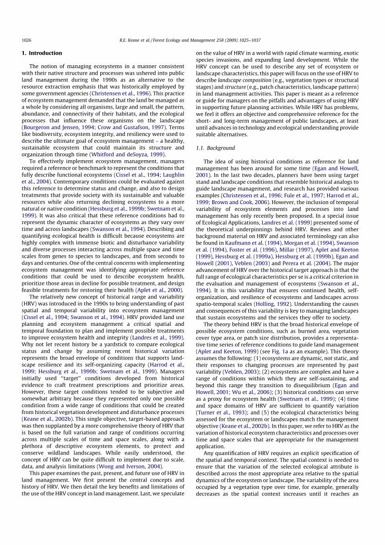
The theory behind HRV is that the broad historical envelope ofpossible ecosystem conditions, such as burned area, vegetationcover type area, or patch size distribution, provides a representa-tive time series of reference conditions to guide land management(Aplet and Keeton, 1999) (see Fig. 1a as an example). This theoryassumes the following: (1) ecosystems are dynamic, not static, andtheir responses to changing processes are represented by pastvariability (Veblen, 2003); (2) ecosystems are complex and have arange of conditions within which they are self-sustaining, andbeyond this range they transition to disequilibrium (Egan andHowell, 2001; Wu et al., 2006); (3) historical conditions can serveas a proxy for ecosystem health (Swetnam et al., 1999); (4) timeand space domains of HRV are sufficient to quantify variation(Turner et al., 1993); and (5) the ecological characteristics beingassessed for the ecosystem or landscapes match the managementobjective (Keane et al., 2002b). In this paper, we refer to HRV as thevariation of historical ecosystem characteristics and processes overtime and space scales that are appropriate for the managementapplication.

Any quantification of HRV requires an explicit specification ofthe spatial and temporal context. The spatial context is needed toensure that the variation of the selected ecological attribute isdescribed across the most appropriate area relative to the spatialdynamics of the ecosystem or landscape. The variability of the areaoccupied by a vegetation type over time, for example, generallydecreases as the spatial context increases until it reaches an

R.E. Keane et al. / Forest Ecology and Management 258 (2009) 1025–10371026

asymptote, which can be used to approximate optimal landscapesize (Fortin and Dale, 2005; Karau and Keane, 2007). The optimalsize of evaluation area will depend on (1) the ecosystem attribute,(2) the dynamics of major disturbance regimes, and (3) themanagement activity being evaluated (Tang and Gustafson,1997). Fine woody fuel loadings, for example, would vary acrosssmaller areas than coarse woody debris loads (Tinker and Knight,2001).

The time scale over which HRV is evaluated must also bespecified to properly interpret the underlying biophysical pro-cesses that influenced historical ecosystem dynamics, especiallyclimate (Millar and Woolfenden, 1999) (Fig. 1b). HRV of landscapecomposition might be entirely different if evaluated from 1000 to1600 A.D. versus 1600 to 1900 A.D. because of the vast differences inclimates between those periods (Mock and Bartlein, 1995).Temporal scale and resolution is usually dictated by the temporaldepth of the historical evidence used to describe HRV but it canalso be selected to match specific management objectives. Thesetwo scale properties are both a benefit and limitation of the HRVconcept (see next sections).

Since it is impossible to quantify all ecosystem characteristicsacross time and space scales, HRV is most effective when confinedto a set of variables that contain the following properties:

� Measurable. The selected variables should be quantifiable acrossthe specified temporal and spatial extent. Insect infestations, for

example, may be difficult to reconstruct over long time periodsfrom historical evidence on the landscape.� Representative. Selected variables should be representative of the

patterns, processes, and characteristics that govern landscapedynamics (i.e., indicator variables). Vegetation type, for example,may be correlated to many other ecosystem characteristics, suchas fire regime, to widen the scope of HRV analysis, or fire historycan serve as a surrogate for vegetation successional status ordisturbance frequency.� Appropriate. Variables must be selected in the context of the

management approach, objective, or application. The HRV of finewoody fuels, for example, may not be appropriate if themanagement activity or proposed action is to enhance wildlifehabitat.

HRV may be used in many phases of land management. Thedeparture of current conditions from historical variations havebeen used to prioritize and select areas for possible restorationtreatments (Reynolds and Hessburg, 2005; Hessburg et al., 2007)or areas to conserve biological diversity (Aplet and Keeton, 1999).US fire management agencies have used Fire Regime ConditionClass (FRCC), based on HRV of fire and vegetation dynamics, to rateand prioritize lands for fuel treatments (Hann and Bunnell, 2001;Schmidt et al., 2002; Hann, 2004) (www.frcc.gov). HRV is used inthe LANDFIRE National Mapping Project to determine departurefrom historical conditions to calculate FRCC across the US at 30 m

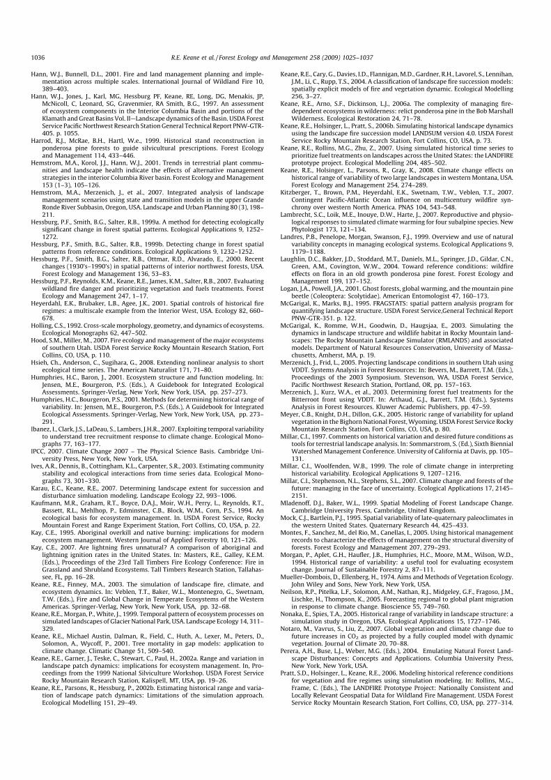
Fig. 1. Examples of time series for quantifying the historical range and variation of landscapes (HRV). (A) A simple example of how the range of a landscape characteristic can

be used as an expression of HRV, (B) an illustration of the HRV for landscape composition for 10,000 ha in western Montana (Keane et al., 2008), (C) a more complex HRV time

series for a 50,000 ha landscape in central Utah (Pratt et al., 2006), and (D) an illustration of how HRV can be altered by a management policy (b), introduction of exotics (c), or

climate change (d).

R.E. Keane et al. / Forest Ecology and Management 258 (2009) 1025–1037 1027

pixel resolution for fire management applications (www.landfir-e.gov). HRV can also be used to design treatments on the landscape.The HRV of patch size and contagion, for example, can be used todesign the size of treatment area and the landscape compositioncan be used to select the appropriate management treatment tomimic patch characteristics (Keane et al., 2002a,b).

Reference conditions for HRV have been described for manyecosystems across the western United States and Canada. Veblenand Donnegan (2005) synthesized available knowledge on forestconditions and ecosystem disturbance for National Forest lands inColorado, USA. The ecological and economic implications of forestpolicies designed to emulate historical fire regimes wereinvestigated by Thompson et al. (2006) using a simulationapproach. Historical vegetation and disturbance dynamics forsouthern Utah were summarized in the Hood and Miller (2007)report. Wong et al. (2003) compiled an extensive reference ofhistorical disturbance regimes for the entire province of BritishColumbia, Canada. Dillon et al. (2005) and Meyer et al. (2005)detail the historical variations in upland vegetation for twonational forests in Wyoming. These efforts are excellent qualitativereferences for understanding and interpreting historical condi-tions, however, they do not provide the quantitative detail neededto implement the described reference conditions directly intomanagement applications (see Fig. 1b,c).

2. Quantifying HRV

A comprehensive quantification of HRV demands temporallydeep, spatially explicit historical data, which is rarely available andoften difficult to obtain (Humphries and Bourgeron, 2001; Barrettet al., 2006) (Fig. 1b,c, for example). Historical reconstructions ofecological processes and attributes can be made from manysources if they exist for the landscape (see Egan and Howell (2001)for a summary). Patterns of fire frequency and severity can befinely to broadly quantified across space and time scales using (1)fire scar dates measured from trees, snags, stumps, and downedlogs, (2) charcoal deposits in soil, lake, and ocean sediments(broad), and (3) burn boundary maps from past and presentsources (Swetnam et al., 1999; Heyerdahl et al., 2001; Humphriesand Bourgeron, 2001). Historical vegetation conditions can bereconstructed or described from (1) pollen deposits in lake orocean sediments, (2) plant macrofossil assemblages deposited inmiddens, sediments, soils, and other sites, (3) dendrochronologicalstand reconstructions, (4) land survey records (Habeck, 1994), and(5) repeat photography (Gruell et al., 1982; Arno et al., 1995;Humphries and Bourgeron, 2001; Friedman and Reich, 2005;Montes et al., 2005; Schulte and Mladenoff, 2005). Unfortunately,these sources can have significant limitations when used todescribe landscape-level HRV in a spatial domain appropriate toland management. These data have either a confined or unknownspatial domain because they were collected on a very small portionof the landscape (i.e., plot or patch), or they pertain to a generalarea (middens, lake sediments) and lack spatial specificity withrespect to patterns. Moreover, some ecosystems on a landscapehave little evidence of past conditions with which to quantify HRVand any available data are usually limited in temporal extent. Ingeneral, those methods that describe HRV at fine time scales, suchas tree fire scar dating, are constrained to multi-centenary timescales, while those methods that cover long time spans (millennia),such as pollen and charcoal analyses, have a resolution that may betoo coarse for management of spatial patterns of structure andcomposition (Swetnam et al., 1999).

For landscape level HRV time series development, there arethree main sources of spatial data to quantify historical conditions(Humphries and Bourgeron, 2001; Keane et al., 2006b). The bestsources are spatial chronosequences or digital maps of landscape

characteristic(s) over many time periods. These maps can bedigitized with GIS software and spatial analysis programs can beused to compute HRV statistics (McGarigal and Marks, 1995).Unfortunately, temporally deep, spatially explicit time series ofhistorical conditions are missing for many US landscapes becauseaerial photography and satellite imagery are rare or non-existentbefore 1930 A.D. and comprehensive maps of forest vegetation arescarce, inconsistent, and limited in coverage prior to 1900 (Keaneet al., 2006b). Tinker et al. (2003) quantified HRV in landscapestructure using digital maps of current and past landscapes in theGreater Yellowstone Area from aerial photos and stand ageinterpretation.

Another HRV data source is to substitute space for time andcollect spatial data across similar landscapes, from one or moretimes, across a large geographic region (Hessburg et al., 1999a,b).Theory posits that if one samples spatial pattern of vegetation ofsimilar biophysical environments with similar disturbance andclimatic regimes, a representative cross section of temporalvariation may be observed. In effect, differences in space areequivalent to differences in time, and inferences may be drawnregarding variation in spatial pattern that might occur at a singlelocation over time. Particularly where process explanation issought, care must be taken in application to select study locationshaving comparable underlying biophysical and climatic condi-tions. However, subtle differences in landform, relief, soils, andclimate make each landscape unique and grouping landscapes maytend to overestimate range and variability of landscape character-istics (Keane et al., 2002a). Landscapes may be similar in terms ofthe processes that govern vegetation, such as climate, disturbance,and species succession, but topography, soils, land use, and winddirection also influence vegetation development and fire growth(Keane et al., 2002b).

A third method of quantifying HRV involves using computermodels to simulate historical dynamics to produce a time series ofsimulated data to compute HRV statistics and metrics (Humphriesand Bourgeron, 2001) (see Fig. 1b). This approach relies on theaccurate simulation of succession and disturbance processes inspace and time (Keane et al., 1999). Many spatially explicitecosystem simulation models are available for quantifying HRVpatch dynamics (for reviews and summaries see Gardner et al.,1999; Mladenoff and Baker, 1999; Humphries and Baron, 2001;Keane and Finney, 2003; Keane et al., 2004), but most are (1)computationally intensive, (2) difficult to parameterize andinitialize, and (3) overly complex, thereby making them difficultto use, especially for large regions, long time periods, andinexperienced staffs. On the other hand, those landscape modelsdesigned specifically for management planning may oversimplifyvegetation development and disturbance (Keane et al., 2004). Eventhe most complex landscape models rarely simulate spatialinteractions between climate, disturbance dynamics, and vegeta-tion development because of the lack of critical research in thoseareas and the immense amount of computer resources required forsuch an effort. Simulation models can include explicit simulationsof climate and human activities to generate more relevant andrealistic estimates of the range and variation of landscapedynamics under today’s conditions. Simulation is the mostcommon method of creating HRV time series.

Many studies have used simulation to quantify HRV for a widevariety of landscapes and ecosystems using a wide variety ofmodels. Non-spatial models, such as VDDT (Beukema and Kurz,1998, were used to estimate landscape composition in a widevariety of areas from the Pacific Northwest to the northern RockyMountains (Hann et al., 1997; Hemstrom et al., 2001, 2007;Merzenich and Frid, 2005; Merzenich et al., 2003). The LADS modelwas used for the Oregon Coast Range to determine the appropriatelevel of old growth forests (Wimberly et al., 2000), to quantify HRV


in landscape structure (Nonaka and Spies, 2005), and to simulatethe effect of forest polices (Thompson et al., 2006). McGarigal et al.(2003) quantified historical forest composition and structures ofColorado landscapes. Keane et al. (2002a) simulated historicallandscape patch dynamics using the LANDSUM model for northernRocky Mountain USA landscapes. As mentioned, the LANDFIREprogram quantifies historical time series for landscapes across theUS using the LANDSUM model (Keane et al., 2007).

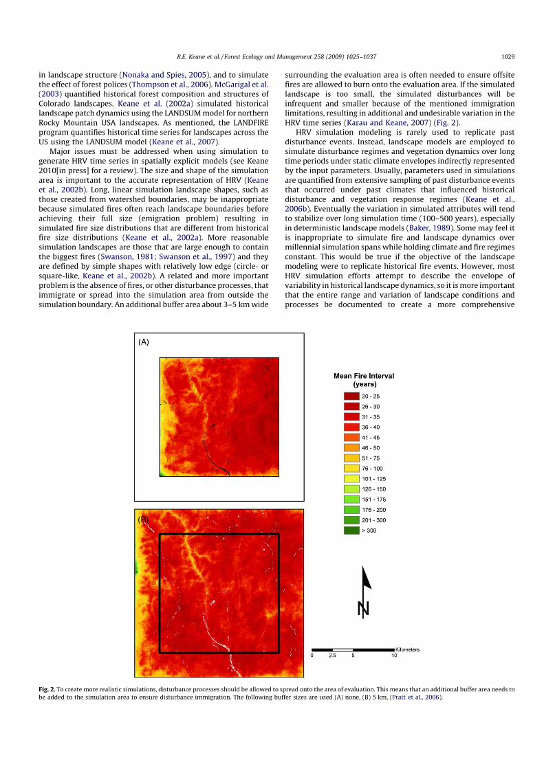
Major issues must be addressed when using simulation togenerate HRV time series in spatially explicit models (see Keane2010[in press] for a review). The size and shape of the simulationarea is important to the accurate representation of HRV (Keaneet al., 2002b). Long, linear simulation landscape shapes, such asthose created from watershed boundaries, may be inappropriatebecause simulated fires often reach landscape boundaries beforeachieving their full size (emigration problem) resulting insimulated fire size distributions that are different from historicalfire size distributions (Keane et al., 2002a). More reasonablesimulation landscapes are those that are large enough to containthe biggest fires (Swanson, 1981; Swanson et al., 1997) and theyare defined by simple shapes with relatively low edge (circle- orsquare-like, Keane et al., 2002b). A related and more importantproblem is the absence of fires, or other disturbance processes, thatimmigrate or spread into the simulation area from outside thesimulation boundary. An additional buffer area about 3–5 km wide

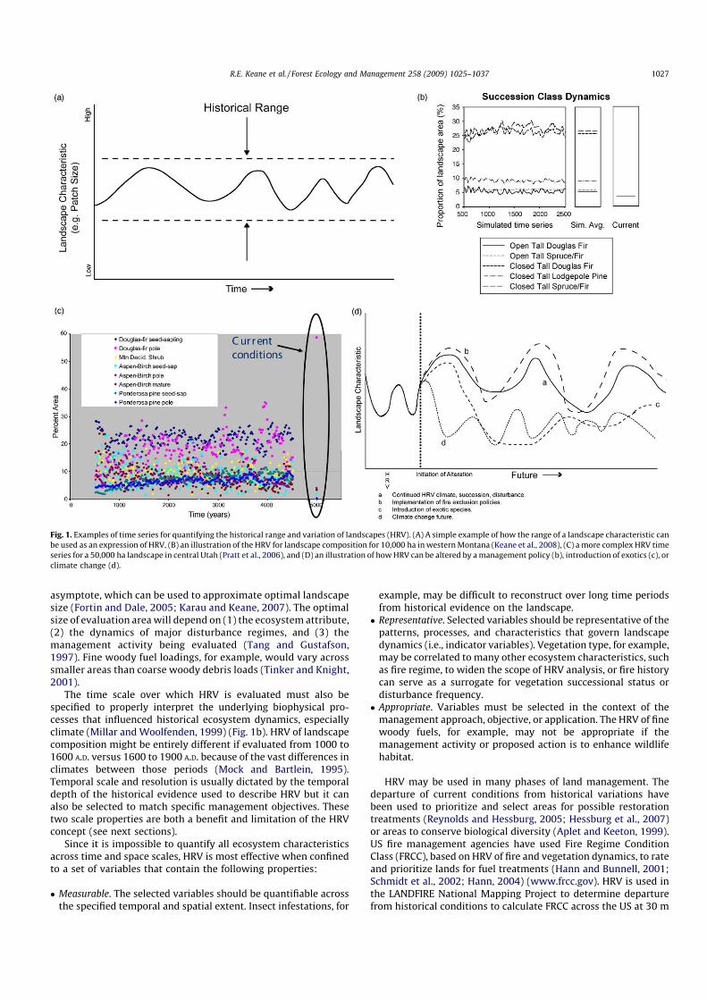
surrounding the evaluation area is often needed to ensure offsitefires are allowed to burn onto the evaluation area. If the simulatedlandscape is too small, the simulated disturbances will beinfrequent and smaller because of the mentioned immigrationlimitations, resulting in additional and undesirable variation in theHRV time series (Karau and Keane, 2007) (Fig. 2).

HRV simulation modeling is rarely used to replicate pastdisturbance events. Instead, landscape models are employed tosimulate disturbance regimes and vegetation dynamics over longtime periods under static climate envelopes indirectly representedby the input parameters. Usually, parameters used in simulationsare quantified from extensive sampling of past disturbance eventsthat occurred under past climates that influenced historicaldisturbance and vegetation response regimes (Keane et al.,2006b). Eventually the variation in simulated attributes will tendto stabilize over long simulation time (100–500 years), especiallyin deterministic landscape models (Baker, 1989). Some may feel itis inappropriate to simulate fire and landscape dynamics overmillennial simulation spans while holding climate and fire regimesconstant. This would be true if the objective of the landscapemodeling were to replicate historical fire events. However, mostHRV simulation efforts attempt to describe the envelope ofvariability in historical landscape dynamics, so it is more importantthat the entire range and variation of landscape conditions andprocesses be documented to create a more comprehensive

Fig. 2. To create more realistic simulations, disturbance processes should be allowed to spread onto the area of evaluation. This means that an additional buffer area needs to

be added to the simulation area to ensure disturbance immigration. The following buffer sizes are used (A) none, (B) 5 km, (Pratt et al., 2006).


reference database. An alternative to simulating long time spans isto conduct simulation replicates using Monte Carlo techniquesproviding the effects of initial conditions are minimized.

The fire history study results that are used to parameterizelandscape models only represent a relatively narrow window oftime (300–400 years), yet it is generally assumed that this smalltemporal span is a good proxy for the creation of referenceconditions used in HRV simulation. Since this window is small, itmay seem that only 400 years of simulation are needed to quantifyHRV. However, the sampled fire events that occurred during thistime represent only one realization of a time series of the initiationand spread of disturbance (fire) events that shaped the uniquelandscapes observed today. If these events had happened on adifferent timetable or in different locations, an entirely new set oflandscape conditions would have resulted. It follows then that thedocumentation of landscape conditions from only historicalrecords would tend to underestimate the historical variabilityof past conditions. Simulation models can quantify the entirerange of conditions by simulating the historical fire regime forthousands of years to capture the full range of possible landscaperealizations.

3. Applying HRV

The operational use of HRV needs a metric or statistic tocompare current landscapes to the historical time series(Fig. 1b,c). This seemingly simple step is actually quite complexfor a number of reasons. First, there are few statistical analysesspecifically designed to evaluate multiple observation historicaltime series and compare against a single observation ofcontemporary conditions. HRV series often contain spatial andtemporal autocorrelation that may influence any parametricstatistical measure of variability (see next section). It is alsodifficult to design a statistic that will meet the needs of managersand match the goal of the HRV analysis. Landscape compositionalthresholds, for example, may be determined as one standarddeviation from the mean for one application, but as the 10th and90th percentile for another (Hann, 2004). Last, there are fewstatistical tests to determine statistical significance of anydifference in a historical-contemporary comparison (Steeleet al., 2006).

Some simulation approaches use the suite of indices that havebeen developed in vegetation ecology for rating the similaritybetween plant communities (Mueller-Dombois and Ellenberg,1974; Gauch, 1982). Hann (2004), for example, used a variation ofthe Sorenson’s Index to compute departure in vegetation condi-tions for an assessment of FRCC. Keane et al. (2008) also usedSorenson’s Index to evaluate the departure of future landscapesfrom historical and current conditions under climate change. TheSorenson’s Index (SI) is:

SI ¼

Xm

j¼1

Xn

i¼1

minðAi;B jÞ

mAreaLRU

0BBBB@

1CCCCA� 100

where the area of a landscape class i, common to both reference A

and simulation output B from simulation output interval j,summed over all landscape classes n and simulation intervals m,

divided by the total area of the landscape reporting unit (AreaLRU)and number of simulation intervals (m), and then converted to apercentage by multiplying by 100. The resulting value has a rangeof 0–100, where 100 is completely similar (identical, no departure)and 0 is completely dissimilar (maximum departure). The problemwith these similarity indices is that they are (1) sensitive tonumber of classes used in the calculation, (2) insensitive to subtle

differences across time intervals, and (3) difficult to implement instatistical analyses and tests for significance.

Steele et al. (2006) took a more statistical approach anddeveloped a program called HRVSTAT that computes departureand a measure of significance using a regression-correlationstrategy. Their program was used in the LANDFIRE prototypeproject to determine ecological departure (Pratt et al., 2006).Cushman and McGarigal (2007) used Principle ComponentsAnalysis to reduce multivariate variability across area by vegeta-tion types to facilitate the measurement of departure from HRV forwildlife applications. Hessburg et al. (1999a, 1999b, 2000) used theFRAGSTATS program and an historical sample median 75 or 80%range of patch and landscape metrics (their estimate of HRV) todetermine departure of contemporary conditions from the HRV.They coupled these estimates with transition analysis, whichenabled them to identify transitions that were responsible forobserved departures, and to detect statistically significant but‘‘nonsense’’ changes resulting from rasterization of historical andcontemporary vegetation coverages in the GIS.

4. Advantages of HRV

One advantage of the HRV approach is that it can be used forsingle or multiple characteristics that describes an ecosystem,stand, or landscape at any scale (Egan and Howell, 2001). The HRVof coarse woody debris loading, for example, can be computed atthe stand, landscape, and regional spatial scale, and similarly, theHRV for landscape composition and patch structure can becomputed for a watershed, National Forest, or an entire region.This multi-scaled, multi-characteristic approach allows HRVattributes to be matched to the specific land managementobjectives at their most appropriate scale. For instance, fuelmanagers might decide to evaluate, at a watershed level, the HRVof coarse woody fuels and severe fire behavior, along with the HRVof landscape contagion (Hessburg et al., 2007), to managelandscapes in favor of continued ecological integrity. Similarly,each HRV element can be prioritized or weighed based on theirimportance to the land management objective. This forms a criticallinkage to adaptive land management where iterative HRVanalyses can be used to balance tradeoffs in landscape integrityof ecosystems with other social issues and economic values.

Another advantage of HRV is that by including the variation ofselected ecosystem attributes in the evaluation analysis, moreflexible, robust, and realistic treatment regimes can be designedsuch that social and economic values are better balanced withecological concerns. The idea that treatments can be scheduled tocreate specific target conditions into the future is flawed because ofthe uncertainty in unplanned disturbances such as wildfires,windstorms, or insect infestations. Instead, land areas could beperiodically evaluated (e.g., every 10 years) using HRV concepts todetermine if they are outside historical ranges, and, if so, appropriatetreatments can be designed to return the evaluated area to asemblance of historical conditions. Planning pro-active treatmentsover long time periods, such as thinnings during harvest rotations,may be unreasonable where disturbance frequencies are short andtheir consequences more severe or variable (Agee, 1997).

Historical conditions need not be the only references for HRVanalyses; other scenarios can be developed and implemented togenerate time series for completely different sets of referenceconditions, such as those that contain extensive domestic livestockgrazing or future climatic change signals (see last section). Theinvasion of late serial native species or exotics may be so extensivethat most of the landscape has semi-permanently departed fromhistorical conditions and it is strictly impractical, both economic-ally and ecologically, to return the landscape to prior conditions.Grazing can be included in the simulation as a dominant


disturbance so that the associated reference condition can bederived. Exotic species may be incorporated into simulationmodels to show alternative pathways of development and theirlikelihood. In other applications, historical reference conditionsmay not be viable for heavily managed areas, such as recreationsites or wildland urban settings, so fire parameters, for example,can be modified to reflect an extensive fire suppression program.Multiple HRV time series can also be created for a wide variety ofresponse variables, such as landscape composition, fuel loadings,and fire behavior. Multiple HRV time series will be very importantfor managing highly altered landscapes, such as those in theeastern US, China, and Europe.

Last, the most important benefit of HRV is the increasedunderstanding about ecosystem dynamics and ecosystemresponses to changing conditions. Understanding the causalmechanisms that drive ecosystem variability is essential ininterpreting HRV analyses, and this understanding allows us toaddress inherent ecological complexity in land management.Exploring the causes underlying the HRV of fire dynamics, forexample, will help design silvicultural treatments that can providesustainable timber products while also reducing fire hazard andreturning ecosystem health (Reinhardt et al., 2008).

5. Limitations of HRV

While HRV seems to have many advantages for use in landmanagement, there are also issues, caveats, and cautions in itsapplication. This section attempts to describe the major problemswith the HRV approach in an order of importance to landmanagement. A thorough knowledge of these HRV limitations iscritical for comprehensive evaluation and interpretation of HRVanalysis results and implementations.

5.1. Limited data

Field data in adequate abundance and appropriately scaled areseldom available to define HRV of characteristics at many scales.On-site historical evidence of past disturbance events or ecologicalconditions is often destroyed by recurrent disturbance ordecomposition, and surviving evidence often lack adequate spatialand temporal distribution and resolution for adequate HRVrepresentation. For example, charcoal samples from varved lakesediments provide an important source of historical data, but thespatial resolution of the data is insufficient for quantifying theannual variation in patterns of fire regimes because the source areafor the deposited charcoal is difficult to define. Fire scars on treesprovide excellent records for the temporal resolution of fires, butscarred trees are rarely distributed across large areas at thedensities needed to adequately describe fire frequency andseverity and the resultant landscape characteristics, especially instand-replacement fire regimes (Baker and Ehle, 2001; Hessburget al., 2007). Many other ecosystems lack the means for recordingdisturbance events (e.g., grass and shrub lands) and our knowledgeof historical trends is necessarily very limited in these systems(Swetnam et al., 1999)

5.2. Autocorrelation

Most historical time series are autocorrelated in space and time(Ives et al., 2003; Hsieh et al., 2008). Any place on a landscape isultimately dependent on the condition of the surrounding area asdisturbance spreads or as water flows through the landscape(Turner, 1987). Related to this that the instantaneous status of anylandscape is dependent on the landscape composition andstructure the previous instant, day, year, and so on with declininginfluence over time (Reed et al., 1998). In addition, the extent of

any vegetation type used to evaluate landscape HRV is related tothe extent of all other vegetation types; any increase in one typemust result in the corresponding decrease of one or more of theother vegetation types (Pratt et al., 2006). It is important tominimize autocorrelation in historical time series by selecting areporting interval that is long enough to reduce the interdepen-dencies of time, space, and succession status but short enough toprovide a sufficient number of observations to compare in a validstatistical test. This reporting interval will vary by landscapedepending on fire frequency and succession transition times. TheLANDFIRE prototype effort used 50-year reporting intervals tominimize autocorrelation for their LANDSUM simulations (Prattet al., 2006). A new set of statistical analysis tools, such as thoseused in economics, are critically needed to compute an index ofdeparture that is useful to land management and satisfies theassumptions of the analysis technique.

5.3. Scale effects

HRV is highly scale-dependent and the range and associatedvariation drifts with pronounced and long-term shifts in theclimatic regime, disturbance regimes, geomorphic and geologicprocesses and also the effects of some human land uses (Morganet al., 1994) (see Fig. 1d). Using a limited temporal and spatialextent to evaluate landscapes across large regions can introducebias into the computation of HRV measures because spatio-temporal variation in the climatic forcing, and vegetation/disturbance responses across a larger domain will typically bebroader than would be observed in a smaller domain. Forexamples, the LANDFIRE prototype time span of 1600 to 1900A.D. (Keane et al., 2007) may be inappropriate for those landscapeswhere fire return intervals are greater than 300 years, and the1 km2 area used to summarize HRV to compute FRCC for nationalfire management concerns (Schmidt et al., 2002) may beinappropriate for areas where the average fire size is greater than1 km2 (Karau and Keane, 2007).

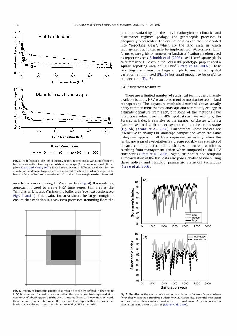
Spatial HRV approaches can be inappropriate when applied onsmall areas such as stands or landforms. Karau and Keane (2007)found that simulated HRV chronosequences summarized fromlandscapes smaller than 100 km2 increased the variability inlandscape composition by over 100% due to the spatial dynamismof simulated disturbance processes (Fig. 3). Thus, quantification ofHRV is likely inappropriate when applied to small areas such asstands or individual landforms. For example, consider a con-temporary 10-ha stand with a Douglas-fir cover type that washistorically dominated by a ponderosa pine cover type; it may beappear to be outside the HRV when considered in isolation, but itwill certainly be within the HRV if it is considered in the context ofa 10,000 to 100,000 ha landscape dominated by ponderosa pine(the historical dominant species). On the other hand, whenevaluation landscapes become too large (>5000 km2), it becomesdifficult to detect significant changes caused by small-scaleecosystem restoration or fuel treatments (Keane et al., 2006b).The optimum size of a HRV landscape reporting area is difficult toestimate because of subtle differences in topography, climate, andvegetation across large regions. Thus, it may be preferable tocompute HRV across spatial scales ranging from 104 to 105 ha,depending upon the question (Karau and Keane, 2007). Theresolution of the landscape is also important with higherresolutions resulting in higher variability (Fig. 3). An alternativemight be to use non-spatial modeling for those areas that are smallor have coarse resolution (Hemstrom et al., 2007; Merzenich andFrid, 2005).

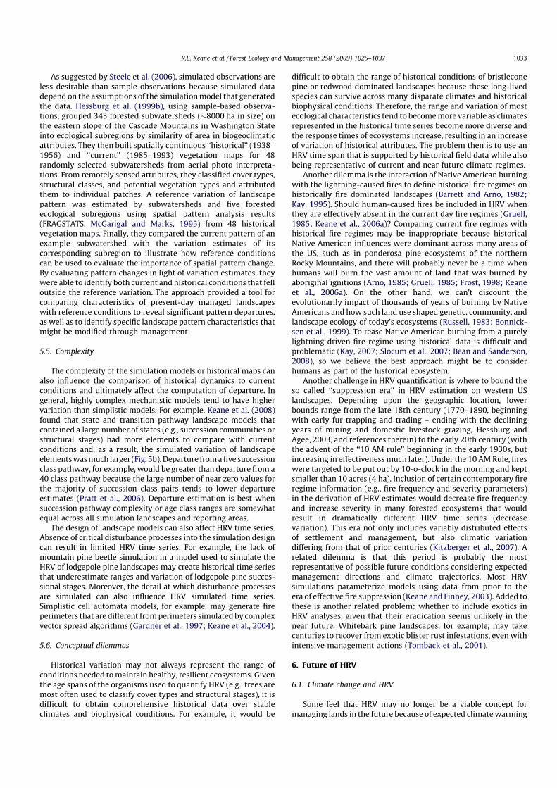
There are several spatial domains that are important in thedevelopment and analysis of HRV time series using spatialmodeling. First is the ‘‘evaluation’’ area defined as the context


area being assessed using HRV approaches (Fig. 4). If a modelingapproach is used to create HRV time series, this area is the‘‘simulation landscape’’ minus the buffer area (see next section; seeFigs. 2 and 4). This evaluation area should be large enough toensure that variation in ecosystem processes stemming from the

inherent variability in the local (subregional) climatic anddisturbance regimes, geology, and geomorphic processes isadequately represented. The evaluation area can then be dividedinto ‘‘reporting areas’’, which are the land units in whichmanagement activities may be implemented. Watersheds, land-forms, square grids, or some other land stratification are often usedas reporting areas. Schmidt et al. (2002) used 1 km2 square pixelsto summarize HRV while the LANDFIRE prototype project used asquare reporting area of 0.81 km2 (Pratt et al., 2006). Thesereporting areas must be large enough to ensure that spatialvariation is minimized (Fig. 3) but small enough to be useful tomanagement (Fig. 2).

5.4. Assessment techniques

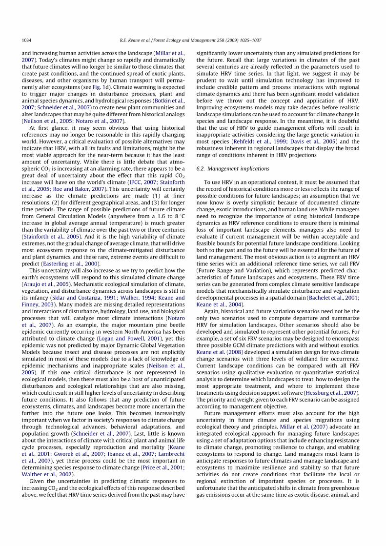
There are a limited number of statistical techniques currentlyavailable to apply HRV as an assessment or monitoring tool in landmanagement. The departure methods described above usuallyapply common metrics from landscape and community ecology toestimate departure from HRV, but some of the methods havelimitations when used in HRV applications. For example, theSorenson’s index is sensitive to the number of classes within afeature used to describe the ecosystem, community, or landscape(Fig. 5b) (Keane et al., 2008). Furthermore, some indices areinsensitive to changes in landscape composition when the samecategories appear in all time sequences, especially when thelandscape areas of a vegetation feature are equal. Many statistics ofdeparture fail to detect subtle changes in current conditionsresulting from management action when compared to the HRVtime series (Pratt et al., 2006). Again, the spatial and temporalautocorrelation of the HRV data also pose a challenge when usingthese indices and standard parametric statistical techniques(Steele et al., 2006).

Fig. 3. The influence of the size of the HRV reporting area on the variation of percent

burned area within two large simulation landscape (A) mountainous and (B) flat

(from Karau and Keane, 2007). Each line represents a different resolution for the

simulation landscape. Larger areas are required to allow disturbance regimes to

become fully realized and the variation of that disturbance regime to be minimized.

Fig. 4. Important landscape extents that must be explicitly defined in developing

HRV time series. The entire area is called the simulation landscape and it is

composed of a buffer (grey) and the evaluation area (black). If modeling is not used,

then the evaluation is often called the reference landscape. Within the evaluation

landscape are the reporting areas for summarizing HRV time series.

Fig. 5. The effect of the number of classes on calculation of Sorenson’s Index where

fewer classes denotes a simulation where only 20 classes (i.e., potential vegetation

and succession class combinations) were used, and more classes represents a

simulation using about 50 classes (Keane et al., 2008).


As suggested by Steele et al. (2006), simulated observations areless desirable than sample observations because simulated datadepend on the assumptions of the simulation model that generatedthe data. Hessburg et al. (1999b), using sample-based observa-tions, grouped 343 forested subwatersheds (�8000 ha in size) onthe eastern slope of the Cascade Mountains in Washington Stateinto ecological subregions by similarity of area in biogeoclimaticattributes. They then built spatially continuous ‘‘historical’’ (1938–1956) and ‘‘current’’ (1985–1993) vegetation maps for 48randomly selected subwatersheds from aerial photo interpreta-tions. From remotely sensed attributes, they classified cover types,structural classes, and potential vegetation types and attributedthem to individual patches. A reference variation of landscapepattern was estimated by subwatersheds and five forestedecological subregions using spatial pattern analysis results(FRAGSTATS, McGarigal and Marks, 1995) from 48 historicalvegetation maps. Finally, they compared the current pattern of anexample subwatershed with the variation estimates of itscorresponding subregion to illustrate how reference conditionscan be used to evaluate the importance of spatial pattern change.By evaluating pattern changes in light of variation estimates, theywere able to identify both current and historical conditions that felloutside the reference variation. The approach provided a tool forcomparing characteristics of present-day managed landscapeswith reference conditions to reveal significant pattern departures,as well as to identify specific landscape pattern characteristics thatmight be modified through management

5.5. Complexity

The complexity of the simulation models or historical maps canalso influence the comparison of historical dynamics to currentconditions and ultimately affect the computation of departure. Ingeneral, highly complex mechanistic models tend to have highervariation than simplistic models. For example, Keane et al. (2008)found that state and transition pathway landscape models thatcontained a large number of states (e.g., succession communities orstructural stages) had more elements to compare with currentconditions and, as a result, the simulated variation of landscapeelements was much larger (Fig. 5b). Departure from a five successionclass pathway, for example, would be greater than departure from a40 class pathway because the large number of near zero values forthe majority of succession class pairs tends to lower departureestimates (Pratt et al., 2006). Departure estimation is best whensuccession pathway complexity or age class ranges are somewhatequal across all simulation landscapes and reporting areas.

The design of landscape models can also affect HRV time series.Absence of critical disturbance processes into the simulation designcan result in limited HRV time series. For example, the lack ofmountain pine beetle simulation in a model used to simulate theHRV of lodgepole pine landscapes may create historical time seriesthat underestimate ranges and variation of lodgepole pine succes-sional stages. Moreover, the detail at which disturbance processesare simulated can also influence HRV simulated time series.Simplistic cell automata models, for example, may generate fireperimeters that are different from perimeters simulated by complexvector spread algorithms (Gardner et al., 1997; Keane et al., 2004).

5.6. Conceptual dilemmas

Historical variation may not always represent the range ofconditions needed to maintain healthy, resilient ecosystems. Giventhe age spans of the organisms used to quantify HRV (e.g., trees aremost often used to classify cover types and structural stages), it isdifficult to obtain comprehensive historical data over stableclimates and biophysical conditions. For example, it would be

difficult to obtain the range of historical conditions of bristleconepine or redwood dominated landscapes because these long-livedspecies can survive across many disparate climates and historicalbiophysical conditions. Therefore, the range and variation of mostecological characteristics tend to become more variable as climatesrepresented in the historical time series become more diverse andthe response times of ecosystems increase, resulting in an increaseof variation of historical attributes. The problem then is to use anHRV time span that is supported by historical field data while alsobeing representative of current and near future climate regimes.

Another dilemma is the interaction of Native American burningwith the lightning-caused fires to define historical fire regimes onhistorically fire dominated landscapes (Barrett and Arno, 1982;Kay, 1995). Should human-caused fires be included in HRV whenthey are effectively absent in the current day fire regimes (Gruell,1985; Keane et al., 2006a)? Comparing current fire regimes withhistorical fire regimes may be inappropriate because historicalNative American influences were dominant across many areas ofthe US, such as in ponderosa pine ecosystems of the northernRocky Mountains, and there will probably never be a time whenhumans will burn the vast amount of land that was burned byaboriginal ignitions (Arno, 1985; Gruell, 1985; Frost, 1998; Keaneet al., 2006a). On the other hand, we can’t discount theevolutionarily impact of thousands of years of burning by NativeAmericans and how such land use shaped genetic, community, andlandscape ecology of today’s ecosystems (Russell, 1983; Bonnick-sen et al., 1999). To tease Native American burning from a purelylightning driven fire regime using historical data is difficult andproblematic (Kay, 2007; Slocum et al., 2007; Bean and Sanderson,2008), so we believe the best approach might be to considerhumans as part of the historical ecosystem.

Another challenge in HRV quantification is where to bound theso called ‘‘suppression era’’ in HRV estimation on western USlandscapes. Depending upon the geographic location, lowerbounds range from the late 18th century (1770–1890, beginningwith early fur trapping and trading – ending with the decliningyears of mining and domestic livestock grazing, Hessburg andAgee, 2003, and references therein) to the early 20th century (withthe advent of the ‘‘10 AM rule’’ beginning in the early 1930s, butincreasing in effectiveness much later). Under the 10 AM Rule, fireswere targeted to be put out by 10-o-clock in the morning and keptsmaller than 10 acres (4 ha). Inclusion of certain contemporary fireregime information (e.g., fire frequency and severity parameters)in the derivation of HRV estimates would decrease fire frequencyand increase severity in many forested ecosystems that wouldresult in dramatically different HRV time series (decreasevariation). This era not only includes variably distributed effectsof settlement and management, but also climatic variationdiffering from that of prior centuries (Kitzberger et al., 2007). Arelated dilemma is that this period is probably the mostrepresentative of possible future conditions considering expectedmanagement directions and climate trajectories. Most HRVsimulations parameterize models using data from prior to theera of effective fire suppression (Keane and Finney, 2003). Added tothese is another related problem: whether to include exotics inHRV analyses, given that their eradication seems unlikely in thenear future. Whitebark pine landscapes, for example, may takecenturies to recover from exotic blister rust infestations, even withintensive management actions (Tomback et al., 2001).

6. Future of HRV

6.1. Climate change and HRV

Some feel that HRV may no longer be a viable concept formanaging lands in the future because of expected climate warming


and increasing human activities across the landscape (Millar et al.,2007). Today’s climates might change so rapidly and dramaticallythat future climates will no longer be similar to those climates thatcreate past conditions, and the continued spread of exotic plants,diseases, and other organisms by human transport will perma-nently alter ecosystems (see Fig. 1d). Climate warming is expectedto trigger major changes in disturbance processes, plant andanimal species dynamics, and hydrological responses (Botkin et al.,2007; Schneider et al., 2007) to create new plant communities andalter landscapes that may be quite different from historical analogs(Neilson et al., 2005; Notaro et al., 2007).

At first glance, it may seem obvious that using historicalreferences may no longer be reasonable in this rapidly changingworld. However, a critical evaluation of possible alternatives mayindicate that HRV, with all its faults and limitations, might be themost viable approach for the near-term because it has the leastamount of uncertainty. While there is little debate that atmo-spheric CO2 is increasing at an alarming rate, there appears to be agreat deal of uncertainty about the effect that this rapid CO2

increase will have on the world’s climate (IPCC, 2007; Stainforthet al., 2005; Roe and Baker, 2007). This uncertainty will certainlyincrease as the climate predictions are made (1) at finerresolutions, (2) for different geographical areas, and (3) for longertime periods. The range of possible predictions of future climatefrom General Circulation Models (anywhere from a 1.6 to 8 8Cincrease in global average annual temperature) is much greaterthan the variability of climate over the past two or three centuries(Stainforth et al., 2005). And it is the high variability of climateextremes, not the gradual change of average climate, that will drivemost ecosystem response to the climate-mitigated disturbanceand plant dynamics, and these rare, extreme events are difficult topredict (Easterling et al., 2000).

This uncertainty will also increase as we try to predict how theearth’s ecosystems will respond to this simulated climate change(Araujo et al., 2005). Mechanistic ecological simulation of climate,vegetation, and disturbance dynamics across landscapes is still inits infancy (Sklar and Costanza, 1991; Walker, 1994; Keane andFinney, 2003). Many models are missing detailed representationsand interactions of disturbance, hydrology, land use, and biologicalprocesses that will catalyze most climate interactions (Notaroet al., 2007). As an example, the major mountain pine beetleepidemic currently occurring in western North America has beenattributed to climate change (Logan and Powell, 2001), yet thisepidemic was not predicted by major Dynamic Global VegetationModels because insect and disease processes are not explicitlysimulated in most of these models due to a lack of knowledge ofepidemic mechanisms and inappropriate scales (Neilson et al.,2005). If this one critical disturbance is not represented inecological models, then there must also be a host of unanticipateddisturbances and ecological relationships that are also missing,which could result in still higher levels of uncertainty in describingfuture conditions. It also follows that any prediction of futureecosystems, climates, and landscapes become more uncertain thefurther into the future one looks. This becomes increasinglyimportant when we factor in society’s responses to climate changethrough technological advances, behavioral adaptations, andpopulation growth (Schneider et al., 2007). Last, little is knownabout the interactions of climate with critical plant and animal lifecycle processes, especially reproduction and mortality (Keaneet al., 2001; Gworek et al., 2007; Ibanez et al., 2007; Lambrechtet al., 2007), yet these process could be the most important indetermining species response to climate change (Price et al., 2001;Walther et al., 2002).

Given the uncertainties in predicting climatic responses toincreasing CO2 and the ecological effects of this response describedabove, we feel that HRV time series derived from the past may have

significantly lower uncertainty than any simulated predictions forthe future. Recall that large variations in climates of the pastseveral centuries are already reflected in the parameters used tosimulate HRV time series. In that light, we suggest it may beprudent to wait until simulation technology has improved toinclude credible pattern and process interactions with regionalclimate dynamics and there has been significant model validationbefore we throw out the concept and application of HRV.Improving ecosystems models may take decades before realisticlandscape simulations can be used to account for climate change inspecies and landscape response. In the meantime, it is doubtfulthat the use of HRV to guide management efforts will result ininappropriate activities considering the large genetic variation inmost species (Rehfeldt et al., 1999; Davis et al., 2005) and therobustness inherent in regional landscapes that display the broadrange of conditions inherent in HRV projections

6.2. Management implications

To use HRV in an operational context, it must be assumed thatthe record of historical conditions more or less reflects the range ofpossible conditions for future landscapes; an assumption that wenow know is overly simplistic because of documented climatechange, exotic introductions, and human land use. While managersneed to recognize the importance of using historical landscapedynamics as HRV reference conditions to ensure there is minimalloss of important landscape elements, managers also need toevaluate if current management will be within acceptable andfeasible bounds for potential future landscape conditions. Lookingboth to the past and to the future will be essential for the future ofland management. The most obvious action is to augment an HRVtime series with an additional reference time series, we call FRV(Future Range and Variation), which represents predicted char-acteristics of future landscapes and ecosystems. These FRV timeseries can be generated from complex climate sensitive landscapemodels that mechanistically simulate disturbance and vegetationdevelopmental processes in a spatial domain (Bachelet et al., 2001;Keane et al., 2004).

Again, historical and future variation scenarios need not be theonly two scenarios used to compute departure and summarizeHRV for simulation landscapes. Other scenarios should also bedeveloped and simulated to represent other potential futures. Forexample, a set of six FRV scenarios may be designed to encompassthree possible GCM climate predictions with and without exotics.Keane et al. (2008) developed a simulation design for two climatechange scenarios with three levels of wildland fire occurrence.Current landscape conditions can be compared with all FRVscenarios using qualitative evaluation or quantitative statisticalanalysis to determine which landscapes to treat, how to design themost appropriate treatment, and where to implement thesetreatments using decision support software (Hessburg et al., 2007).The priority and weight given to each FRV scenario can be assignedaccording to management objective.

Future management efforts must also account for the highuncertainty in future climate and species migrations usingecological theory and principles. Millar et al. (2007) advocate anintegrated ecological approach for managing future landscapesusing a set of adaptation options that include enhancing resistanceto climate change, promoting resilience to change, and enablingecosystems to respond to change. Land managers must learn toanticipate responses to future climates and manage landscape andecosystems to maximize resilience and stability so that futureactivities do not create conditions that facilitate the local orregional extinction of important species or processes. It isunfortunate that the anticipated shifts in climate from greenhousegas emissions occur at the same time as exotic disease, animal, and


plant species invasions and decades of fire suppression. Tempertonet al. (2004) believes that there is no ideal reference for anyecosystem or landscape, but historical context must be consideredto determine reasonable reference states. They advocate thatassembly rules (ecological restrictions on the observed patterns ofspecies dynamics) could be used to construct plausible restorationor management goals, especially under rapid climate change.

In closing, we feel it is important to mention that future landmanagement and society will also require a brand new land ethicto provide context in which to make land management decisions. Ifexpected biotic responses to climate change come true, tomor-row’s landscapes will be so altered by human actions that currentmanagement philosophies and policies of managing for healthyecosystems, wilderness conditions, or historical analogs will nolonger be feasible because these objectives will be impossible toachieve in the future. Will the elimination of exotic plants anddiseases, for example, still be an important management objectiveif we know that other novel plant communities may inhabittomorrow’s landscapes. A new management approach may beneeded to balance ecology principles with society’s demand forresource to create landscapes that are sustainable, ecologicalviable, and acceptable to society. Using assembly rules to restorelandscapes may offer a possible direction (Temperton et al., 2004).Conserving historical landscape features while also providing forfuture species migrations and changes in disturbance regimes maybe another strategy. In the end, this may require a totally differentland ethic than we used to guide management in the past (e.g., firesuppression). Such an ethic will most likely require that we moreexplicitly identify the goals we intend to fulfill, and how and wherethese goals can be integrated across the landscape.

Acknowledgements

This paper was written as a result of a HRV and climate changeworkshop held April 2008 in Washington, DC, USA and sponsoredby The Nature Conservancy and USDA Forest Service. We thankthose participants for their discussion and ideas.

References

Agee, J.K., 1997. Fire management for the 21st century. In: Kohm, K.A., Franklin, J.F.(Eds.), Creating A Forestry for the 21st Century: The Science of EcosystemManagement. Island Press, Washington, DC, pp. 191–201.

Aplet, G., Keeton, W.S., 1999. Application of historical range of variability con-cepts to biodiversity conservation. In: Baydack, R.K., Campa, H., Haufler, J.B.(Eds.), Practical Approaches to the Conservation of Biological Diversity. IslandPress, NY, New York, pp. 71–86.

Aplet, G., Thomson, J., Wilbert, M., 2000. Indicators of wildness: using attributes of theland to assess the context of wilderness. In: McCool, S.F., Cole, D.N., Borrie, W.T.,O’Loughlin, J. (Eds.), Wilderness Science in a Time of Change. USDA Forest ServiceRocky Mountain Research Station, RMRS-P-15-VOL-2, Missoula, MT, pp. 89–98.

Araujo, M.B., Whittaker, R.J., Ladle, R.J., Erhard, M., 2005. Reducing uncertainty inprojections of extinction risk from climate change. Global Ecology and Biogeo-graphy Letters 14, 529–538.

Arno, S.F., 1985. Ecological effects and management implications of Indian fires. In:Lotan, J.E., Kilgore, B.M. Fischer, W.C., Mutch, R.W. (tech. coordinators) (Eds.),Proceedings of the Symposium and Workshop on Wilderness Fire. USDA ForestService General Technical Report INT-182, pp. 81–89.

Arno, S.F., Scott, J.H., Hartwell, M.G., 1995. Age-Class Structure of Old GrowthPonderosa Pine/Douglas-fir Stands and its Relationship to Fire History. Inter-mountain Research Station, Forest Service, USDA.

Bachelet, D., Neilson, R.P., Lenihan, J.M., Drapek, R.J., 2001. Climate change effects onvegetation distribution and carbon budget in the United States. Ecosystems 4,164–185.

Baker, W.L., 1989. A review of models of landscape change. Landscape Ecology 2,111–133.

Baker, W.L., Ehle, D., 2001. Uncertainty in surface-fire history: the case of ponderosapine forests in the western United States. Canadian Journal of Forest Research31, 1205–1226.

Barrett, S.W., Arno, S.F., 1982. Indian fires as an ecological influence in the northernRockies. Journal of Forestry 647–651.

Barrett, S.W., DeMeo, T., Jones, J.L., Zeiler, J.D., Hutter, L.C., 2006. Assessing ecologicaldeparture from reference conditions with the Fire Regime Condition Class

(FRCC) mapping tool. In: Andrews, P.L., Butler, B.W. (Eds.), Fuels Management– How to Measure Success. USDA Forest Service Rocky Mountain ResearchStation, Portland, OR, USA, pp. 575–585.

Bean, W.T., Sanderson, E.W., 2008. Using a spatially explicit ecological model to testscenarios of fire use by Native Americans: an example from the Harlem Plains,New York, NY. Ecological Modelling 211, 301–308.

Beukema, S.J., Kurz, W.A., 1998. Vegetation dynamics development tool – usersGuide Version 3.0. ESSA Technologies, #300-1765 West 8th Avenue, Vancouver,BC, Canada.

Bonnicksen, T.M., Anderson, M.K., Lewis, H.T., Kay, C.E., Knudson, R., 1999. NativeAmerican influences on the development of forest ecosystems. In: Szaro, R.C.,Johnson, N.C., Sexton, W.T., Malk, A.J. (Eds.), Ecological Stewardship: A CommonReference for Ecosystem Management, pp. 439–470.

Botkin, D.B., Saxe, H., Araujo, M.B., Betts, R., Bradshaw, R.W., Cedhagen, T., others, A.,2007. Forecasting the effects of global warming on biodiversity. Bioscience 57,227–236.

Bourgeron, P.S., Jensen, M.E., 1994. An overview of ecological principles for eco-system management. In: Jensen, M.E., Bourgeron, P.S. (Eds.), Ecosystem Man-agement: Principles and Applications. U.S. Department of Agriculture, ForestService, Pacific Northwest Research Station, Portland, Oregon, pp. 45–57.

Brown, P.M., Cook, B., 2006. Early settlement forest structure in Black Hills ponder-osa pine forests. Forest Ecology and Management 223, 284–290.

Christensen, N.L., Bartuska, A.M., Brown, J.H., Carpenter, S., D’Antonio, C., Francis, R.,Franklin, J.F., MacMahon, J.A., Noss, R.F., Parsons, D.J., Peterson, C.H., Turner,M.G., Woodmansee, R.G., 1996. The report of the ecological society of Americacommittee on the scientific basis for ecosystem management. Ecological Appli-cations 6, 665–691.

Cissel, J.H., Swanson, F.J., McKee, W.A., Burditt, A.L., 1994. Using the past to plan thefuture in the Pacific Northwest. Journal of Forestry 92 (30–31), 46.

Crow, T.R., Gustafson, E.J., 1997. Ecosystem management: managing naturalresources in time and space. In: Kohm, K.A., Franklin, J.F. (Eds.), CreatingForestry for the 21st Century. Island Press, Washington, DC, USA, pp. 215–229.

Cushman, S.A., McGarigal, K., 2007. Multivariate landscape trajectory analysis: anexample using simulation modeling of American Marten habitat change underfour timber harvest scenarios. In: Bissonette, J.A., Storch, I. (Eds.), TemporalDimensions of Landscape Ecology Wildlife Responses to Variable Resources.Springer, US, pp. 119–140.

Davis, M.B., Shaw, R.G., Etterson, J.R., 2005. Evolutionary responses to changingclimates. Ecology 86, 1704–1714.

Dillon, G.K., Knight, D.H., Meyer, C.B., 2005. Historic range of variability for uplandvegetation in the Medicine Bow National Forest, Wyoming. USDA Forest ServiceRocky Mountain Research Station, Fort Collins, CO, USA, p. 85.

Easterling, D.R., Meehl, G.A., Parmesan, C., Changnon, S.A., Karl, T.R., Mearns, L.O.,2000. Climate extremes: observations, modeling, and impacts. Science 289,2068–2074.

Egan, D., Howell, E.A. (Eds.), 2001. The Historical Ecology Handbook. Island Press,Washington, DC, USA.

Fortin, M.J., Dale, M.R., 2005. Spatial Analysis: A Guide for Ecologists. CambridgeUniversity Press, Cambridge, United Kingdom.

Foster, D.R., Orwig, D.A., McLachlan, J.S., 1996. Ecological and conservation insightsfrom reconstructive studies of temperate old-growth forests. Trends in Ecologyand Evolution 11, 419–425.

Friedman, S.K., Reich, P.B., 2005. Regional legacies of logging: departure frompresettlement forest conditions in northern Minnesota. Ecological Applications15, 726–744.

Frost, C.C., 1998. Presettlement fire frequency regimes of the United States: a firstapproximation. Tall Timbers Fire Ecology Conference 20, 70–81.

Fule, P.Z., Covington, W.W., Moore, M.M., 1997. Determining reference conditionsfor ecosystem management of southwestern ponderosa pine forests. EcologicalApplications 7, 895–908.

Gardner, R.H.R., William, H., Turner Monica, G., 1997. Effects of scale-dependentprocesses on predicting patterns of forest fires. In: Walker, B.H., Steffen, W.L.(Eds.), Global Change and Terrestrial Ecosystems. Cambridge, UK, pp. 111–134.

Gardner, R.H., William, H., Romme, Turner, M.G., 1999. Predicting forest fire effectsat landscape scales. In: Mladenoff, D.J., Baker, W.L. (Eds.), Spatial Modeling ofForest Landscape Change: Approaches and Applications. Cambridge UniversityPress, Cambridge, United Kingdom, pp. 163–185.

Gauch, H.G., 1982. Multivariate Analysis in Community Ecology. Cambridge Uni-versity Press, New York, New York, USA.

Gruell, G.E., 1985. Indian fires in the interior west: a widespread influence. In: Lotan,J.E., Kilgore, B.M., Fischer, W.C. (Coordinators), R.W.M.t. (Eds.), Proceedings of theSymposium and Workshop on Wilderness Fire. USDA Forest Service, pp. 62–74.

Gruell, G.E., Schmidt, W.C., Arno, S.F., Reich, W.J., 1982. Seventy years of vegetativechange in a managed ponderosa pine forest in western Montana—implicationsfor resource management. USDA Forest Service, Intermountain Forest andRange Experiment Station, Ogden, UT, p. 41.

Gworek, J.R., Vander Wall, S.B., Brussard, P.F., 2007. Changes in biotic interactionsand climate determine recruitment of Jeffrey pine along an elevation gradient.Forest Ecology and Management 239, 57–68.

Habeck, J.R., 1994. Using General Land Office records to assess forest succession inponderosa pine-Douglas-fir forests in western Montana. Northwest Science 68,69–78.

Hann, W.J., 2004. Mapping fire regime condition class: a method for watershedand project scale analysis. In: Engstrom, R.T., Galley, K.E.M., De Groot, W.J.(Eds.), 22nd Tall Timbers Fire Ecology Conference: Fire in Temperate, Boreal,and Montane Ecosystems. Tall Timbers Research Station, pp. 22–44.


Hann, W.J., Bunnell, D.L., 2001. Fire and land management planning and imple-mentation across multiple scales. International Journal of Wildland Fire 10,389–403.

Hann, W.J., Jones, J., Karl, MG, Hessburg PF, Keane, RE, Long, DG, Menakis, JP,McNicoll, C, Leonard, SG, Gravenmier, RA Smith, B.G., 1997. An assessmentof ecosystem components in the Interior Columbia Basin and portions of theKlamath and Great Basins Vol. II—Landscape dynamics of the Basin. USDA ForestService Pacific Northwest Research Station General Technical Report PNW-GTR-405. p. 1055.

Harrod, R.J., McRae, B.H., Hartl, W.e., 1999. Historical stand reconstruction inponderosa pine forests to guide silvicultural prescriptions. Forest Ecologyand Management 114, 433–446.

Hemstrom, M.A., Korol, J.J., Hann, W.J., 2001. Trends in terrestrial plant commu-nities and landscape health indicate the effects of alternative managementstrategies in the interior Columbia River basin. Forest Ecology and Management153 (1–3), 105–126.

Hemstrom, M.A., Merzenich, J., et al., 2007. Integrated analysis of landscapemanagement scenarios using state and transition models in the upper GrandeRonde River Subbasin, Oregon, USA. Landscape and Urban Planning 80 (3), 198–211.

Hessburg, P.F., Smith, B.G., Salter, R.B., 1999a. A method for detecting ecologicallysignificant change in forest spatial patterns. Ecological Applications 9, 1252–1272.

Hessburg, P.F., Smith, B.G., Salter, R.B., 1999b. Detecting change in forest spatialpatterns from reference conditions. Ecological Applications 9, 1232–1252.

Hessburg, P.F., Smith, B.G., Salter, R.B., Ottmar, R.D., Alvarado, E., 2000. Recentchanges (1930’s–1990’s) in spatial patterns of interior northwest forests, USA.Forest Ecology and Management 136, 53–83.

Hessburg, P.F., Reynolds, K.M., Keane, R.E., James, K.M., Salter, R.B., 2007. Evaluatingwildland fire danger and prioritizing vegetation and fuels treatments. ForestEcology and Management 247, 1–17.

Heyerdahl, E.K., Brubaker, L.B., Agee, J.K., 2001. Spatial controls of historical fireregimes: a multiscale example from the Interior West, USA. Ecology 82, 660–678.

Holling, C.S., 1992. Cross-scale morphology, geometry, and dynamics of ecosystems.Ecological Monographs 62, 447–502.

Hood, S.M., Miller, M., 2007. Fire ecology and management of the major ecosystemsof southern Utah. USDA Forest Service Rocky Mountain Research Station, FortCollins, CO, USA, p. 110.

Hsieh, Ch., Anderson, C., Sugihara, G., 2008. Extending nonlinear analysis to shortecological time series. The American Naturalist 171, 71–80.

Humphries, H.C., Baron, J., 2001. Ecosystem structure and function modeling. In:Jensen, M.E., Bourgeron, P.S. (Eds.), A Guidebook for Integrated EcologicalAssessments. Springer-Verlag, New York, New York, USA, pp. 257–273.

Humphries, H.C., Bourgeron, P.S., 2001. Methods for determining historical range ofvariability. In: Jensen, M.E., Bourgeron, P.S. (Eds.), A Guidebook for IntegratedEcological Assessments. Springer-Verlag, New York, New York, USA, pp. 273–291.

Ibanez, I., Clark, J.S., LaDeau, S., Lambers, J.H.R., 2007. Exploiting temporal variabilityto understand tree recruitment response to climate change. Ecological Mono-graphs 77, 163–177.

IPCC, 2007. Climate Change 2007 – The Physical Science Basis. Cambridge Uni-versity Press, New York, New York, USA.

Ives, A.R., Dennis, B., Cottingham, K.L., Carpenter, S.R., 2003. Estimating communitystability and ecological interactions from time series data. Ecological Mono-graphs 73, 301–330.

Karau, E.C., Keane, R.E., 2007. Determining landscape extent for succession anddisturbance simluation modeling. Landscape Ecology 22, 993–1006.

Kaufmann, M.R., Graham, R.T., Boyce, D.A.J., Moir, W.H., Perry, L., Reynolds, R.T.,Bassett, R.L., Mehlhop, P., Edminster, C.B., Block, W.M., Corn, P.S., 1994. Anecological basis for ecosystem management. In. USDA Forest Service, RockyMountain Forest and Range Experiment Station, Fort Collins, CO, USA, p. 22.

Kay, C.E., 1995. Aboriginal overkill and native burning: implications for modernecosystem management. Western Journal of Applied Forestry 10, 121–126.

Kay, C.E., 2007. Are lightning fires unnatural? A comparison of aboriginal andlightning ignition rates in the United States. In: Masters, R.E., Galley, K.E.M.(Eds.), Proceedings of the 23rd Tall Timbers Fire Ecology Conference: Fire inGrassland and Shrubland Ecosystems. Tall Timbers Research Station, Tallahas-see, FL, pp. 16–28.

Keane, R.E., Finney, M.A., 2003. The simulation of landscape fire, climate, andecosystem dynamics. In: Veblen, T.T., Baker, W.L., Montenegro, G., Swetnam,T.W. (Eds.), Fire and Global Change in Temperate Ecosystems of the WesternAmericas. Springer-Verlag, New York, New York, USA, pp. 32–68.

Keane, R.E., Morgan, P., White, J., 1999. Temporal pattern of ecosystem processes onsimulated landscapes of Glacier National Park, USA. Landscape Ecology 14, 311–329.

Keane, R.E., Michael Austin, Dalman, R., Field, C., Huth, A., Lexer, M., Peters, D.,Solomon, A., Wycoff, P., 2001. Tree mortality in gap models: application toclimate change. Climatic Change 51, 509–540.

Keane, R.E., Garner, J., Teske, C., Stewart, C., Paul, H., 2002a. Range and variation inlandscape patch dynamics: implications for ecosystem management. In, Pro-ceedings from the 1999 National Silviculture Workshop. USDA Forest ServiceRocky Mountain Research Station, Kalispell, MT, USA, pp. 19–26.

Keane, R.E., Parsons, R., Hessburg, P., 2002b. Estimating historical range and varia-tion of landscape patch dynamics: Limitations of the simulation approach.Ecological Modelling 151, 29–49.

Keane, R.E., Cary, G., Davies, I.D., Flannigan, M.D., Gardner, R.H., Lavorel, S., Lennihan,J.M., Li, C., Rupp, T.S., 2004. A classification of landscape fire succession models:spatially explicit models of fire and vegetation dynamic. Ecological Modelling256, 3–27.

Keane, R.E., Arno, S.F., Dickinson, L.J., 2006a. The complexity of managing fire-dependent ecosystems in wilderness: relict ponderosa pine in the Bob MarshallWilderness. Ecological Restoration 24, 71–78.

Keane, R.E., Holsinger, L., Pratt, S., 2006b. Simulating historical landscape dynamicsusing the landscape fire succession model LANDSUM version 4.0. USDA ForestService Rocky Mountain Research Station, Fort Collins, CO, USA, p. 73.

Keane, R.E., Rollins, M.G., Zhu, Z., 2007. Using simulated historical time series toprioritize fuel treatments on landscapes across the United States: the LANDFIREprototype project. Ecological Modelling 204, 485–502.

Keane, R.E., Holsinger, L., Parsons, R., Gray, K., 2008. Climate change effects onhistorical range of variability of two large landscapes in western Montana, USA.Forest Ecology and Management 254, 274–289.

Kitzberger, T., Brown, P.M., Heyerdahl, E.K., Swetnam, T.W., Veblen, T.T., 2007.Contingent Pacific-Atlantic Ocean influence on multicentury wildfire syn-chrony over western North America. PNAS 104, 543–548.

Lambrecht, S.C., Loik, M.E., Inouye, D.W., Harte, J., 2007. Reproductive and physio-logical responses to simulated climate warming for four subalpine species. NewPhytologist 173, 121–134.

Landres, P.B., Penelope, Morgan, Swanson, F.J., 1999. Overview and use of naturalvariability concepts in managing ecological systems. Ecological Applications 9,1179–1188.

Laughlin, D.C., Bakker, J.D., Stoddard, M.T., Daniels, M.L., Springer, J.D., Gildar, C.N.,Green, A.M., Covington, W.W., 2004. Toward reference conditions: wildfireeffects on flora in an old growth ponderosa pine forest. Forest Ecology andManagement 199, 137–152.

Logan, J.A., Powell, J.A., 2001. Ghost forests, global warming, and the mountain pinebeetle (Coleoptera: Scolytidae). American Entomologist 47, 160–173.

McGarigal, K., Marks, B.J., 1995. FRAGSTATS: spatial pattern analysis program forquantifying landscape structure. USDA Forest Service,General Technical ReportPNW-GTR-351. p. 122.

McGarigal, K., Romme, W.H., Goodwin, D., Haugsjaa, E., 2003. Simulating thedynamics in landscape structure and wildlife habitat in Rocky Mountain land-scapes: The Rocky Mountain Landscape Simulator (RMLANDS) and associatedmodels. Department of Natural Resources Conservation, University of Massa-chusetts, Amherst, MA, p. 19.

Merzenich, J., Frid, L., 2005. Projecting landscape conditions in southern Utah usingVDDT. Systems Analysis in Forest Resources: In: Bevers, M., Barrett, T.M. (Eds.),Proceedings of the 2003 Symposium. Stevenson, WA, USDA Forest Service,Pacific Northwest Research Station, Portland, OR, pp. 157–163.

Merzenich, J., Kurz, W.A., et al., 2003. Determining forest fuel treatments for theBitterroot front using VDDT. In: Arthaud, G.J., Barrett, T.M. (Eds.), SystemsAnalysis in Forest Resources. Kluwer Academic Publishers, pp. 47–59.

Meyer, C.B., Knight, D.H., Dillon, G.K., 2005. Historic range of variability for uplandvegetation in the Bighorn National Forest, Wyoming. USDA Forest Service RockyMountain Research Station, Fort Collins, CO, USA, p. 80.

Millar, C.I., 1997. Comments on historical variation and desired future conditions astools for terrestrial landscape analysis. In: Sommarstrom, S. (Ed.), Sixth BiennialWatershed Management Conference. University of California at Davis, pp. 105–131.

Millar, C.I., Woolfenden, W.B., 1999. The role of climate change in interpretinghistorical variability. Ecological Applications 9, 1207–1216.

Millar, C.I., Stephenson, N.L., Stephens, S.L., 2007. Climate change and forests of thefuture: managing in the face of uncertainty. Ecological Applications 17, 2145–2151.

Mladenoff, D.J., Baker, W.L., 1999. Spatial Modeling of Forest Landscape Change.Cambridge University Press, Cambridge, United Kingdom.

Mock, C.J., Bartlein, P.J., 1995. Spatial variability of late-quaternary paleoclimates inthe western United States. Quaternary Research 44, 425–433.

Montes, F., Sanchez, M., del Rio, M., Canellas, I., 2005. Using historical managementrecords to characterize the effects of management on the structural diversity offorests. Forest Ecology and Management 207, 279–293.

Morgan, P., Aplet, G.H., Haufler, J.B., Humphries, H.C., Moore, M.M., Wilson, W.D.,1994. Historical range of variability: a useful tool for evaluating ecosystemchange. Journal of Sustainable Forestry 2, 87–111.

Mueller-Dombois, D., Ellenberg, H., 1974. Aims and Methods of Vegetation Ecology.John Wiley and Sons, New York, New York, USA.

Neilson, R.P., Pitelka, L.F., Solomon, A.M., Nathan, R.J., Midgeley, G.F., Fragoso, J.M.,Lischke, H., Thompson, K., 2005. Forecasting regional to global plant migrationin response to climate change. Bioscience 55, 749–760.

Nonaka, E., Spies, T.A., 2005. Historical range of variability in landscape structure: asimulation study in Oregon, USA. Ecological Applications 15, 1727–1746.

Notaro, M., Vavrus, S., Liu, Z., 2007. Global vegetation and climate change due tofuture increases in CO2 as projected by a fully coupled model with dynamicvegetation. Journal of Climate 20, 70–88.

Perera, A.H., Buse, L.J., Weber, M.G. (Eds.), 2004. Emulating Natural Forest Land-scape Disturbances: Concepts and Applications. Columbia University Press,New York, New York, USA.

Pratt, S.D., Holsinger, L., Keane, R.E., 2006. Modeling historical reference conditionsfor vegetation and fire regimes using simulation modeling. In: Rollins, M.G.,Frame, C. (Eds.), The LANDFIRE Prototype Project: Nationally Consistent andLocally Relevant Geospatial Data for Wildland Fire Management. USDA ForestService Rocky Mountain Research Station, Fort Collins, CO, USA, pp. 277–314.


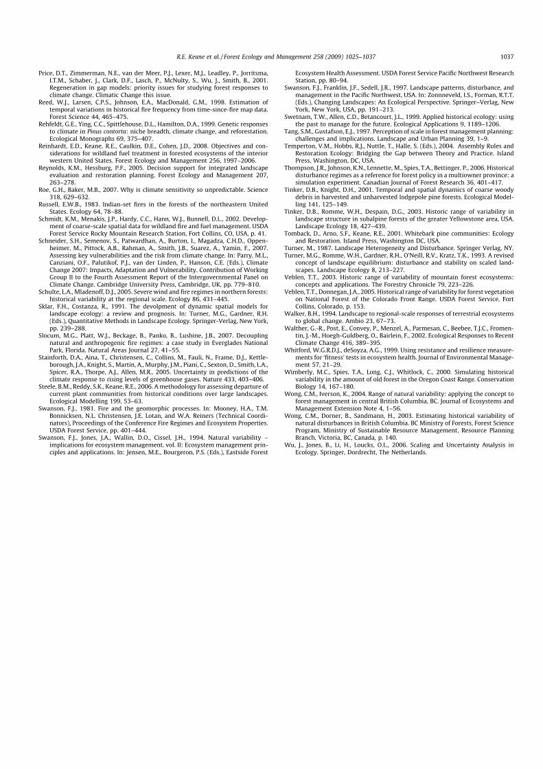
Price, D.T., Zimmerman, N.E., van der Meer, P.J., Lexer, M.J., Leadley, P., Jorritsma,I.T.M., Schaber, J., Clark, D.F., Lasch, P., McNulty, S., Wu, J., Smith, B., 2001.Regeneration in gap models: priority issues for studying forest responses toclimate change. Climatic Change this issue.

Reed, W.J., Larsen, C.P.S., Johnson, E.A., MacDonald, G.M., 1998. Estimation oftemporal variations in historical fire frequency from time-since-fire map data.Forest Science 44, 465–475.

Rehfeldt, G.E., Ying, C.C., Spittlehouse, D.L., Hamilton, D.A., 1999. Genetic responsesto climate in Pinus contorta: niche breadth, climate change, and reforestation.Ecological Monographs 69, 375–407.

Reinhardt, E.D., Keane, R.E., Caulkin, D.E., Cohen, J.D., 2008. Objectives and con-siderations for wildland fuel treatment in forested ecosystems of the interiorwestern United States. Forest Ecology and Management 256, 1997–2006.

Reynolds, K.M., Hessburg, P.F., 2005. Decision support for integrated landscapeevaluation and restoration planning. Forest Ecology and Management 207,263–278.

Roe, G.H., Baker, M.B., 2007. Why is climate sensitivity so unpredictable. Science318, 629–632.

Russell, E.W.B., 1983. Indian-set fires in the forests of the northeastern UnitedStates. Ecology 64, 78–88.

Schmidt, K.M., Menakis, J.P., Hardy, C.C., Hann, W.J., Bunnell, D.L., 2002. Develop-ment of coarse-scale spatial data for wildland fire and fuel management. USDAForest Service Rocky Mountain Research Station, Fort Collins, CO, USA, p. 41.

Schneider, S.H., Semenov, S., Patwardhan, A., Burton, I., Magadza, C.H.D., Oppen-heimer, M., Pittock, A.B., Rahman, A., Smith, J.B., Suarez, A., Yamin, F., 2007.Assessing key vulnerabilities and the risk from climate change. In: Parry, M.L.,Canziani, O.F., Palutikof, P.J., van der Linden, P., Hanson, C.E. (Eds.), ClimateChange 2007: Impacts, Adaptation and Vulnerability. Contribution of WorkingGroup II to the Fourth Assessment Report of the Intergovernmental Panel onClimate Change. Cambridge University Press, Cambridge, UK, pp. 779–810.

Schulte, L.A., Mladenoff, D.J., 2005. Severe wind and fire regimes in northern forests:historical variability at the regional scale. Ecology 86, 431–445.

Sklar, F.H., Costanza, R., 1991. The devolpment of dynamic spatial models forlandscape ecology: a review and prognosis. In: Turner, M.G., Gardner, R.H.(Eds.), Quantitative Methods in Landscape Ecology. Springer-Verlag, New York,pp. 239–288.

Slocum, M.G., Platt, W.J., Beckage, B., Panko, B., Lushine, J.B., 2007. Decouplingnatural and anthropogenic fire regimes: a case study in Everglades NationalPark, Florida. Natural Areas Journal 27, 41–55.

Stainforth, D.A., Aina, T., Christensen, C., Collins, M., Fauli, N., Frame, D.J., Kettle-borough, J.A., Knight, S., Martin, A., Murphy, J.M., Piani, C., Sexton, D., Smith, L.A.,Spicer, R.A., Thorpe, A.J., Allen, M.R., 2005. Uncertainty in predictions of theclimate response to rising levels of greenhouse gases. Nature 433, 403–406.

Steele, B.M., Reddy, S.K., Keane, R.E., 2006. A methodology for assessing departure ofcurrent plant communities from historical conditions over large landscapes.Ecological Modelling 199, 53–63.

Swanson, F.J., 1981. Fire and the geomorphic processes. In: Mooney, H.A., T.M.Bonnicksen, N.L. Christensen, J.E. Lotan, and W.A. Reiners (Technical Coordi-nators), Proceedings of the Conference Fire Regimes and Ecosystem Properties.USDA Forest Service, pp. 401–444.

Swanson, F.J., Jones, J.A., Wallin, D.O., Cissel, J.H., 1994. Natural variability –implications for ecosystem management. vol. II: Ecosystem management prin-ciples and applications. In: Jensen, M.E., Bourgeron, P.S. (Eds.), Eastside Forest

Ecosystem Health Assessment. USDA Forest Service Pacific Northwest ResearchStation, pp. 80–94.

Swanson, F.J., Franklin, J.F., Sedell, J.R., 1997. Landscape patterns, disturbance, andmanagement in the Pacific Northwest, USA. In: Zonnneveld, I.S., Forman, R.T.T.(Eds.), Changing Landscapes: An Ecological Perspective. Springer–Verlag, NewYork, New York, USA, pp. 191–213.

Swetnam, T.W., Allen, C.D., Betancourt, J.L., 1999. Applied historical ecology: usingthe past to manage for the future. Ecological Applications 9, 1189–1206.

Tang, S.M., Gustafson, E.J., 1997. Perception of scale in forest management planning:challenges and implications. Landscape and Urban Planning 39, 1–9.

Temperton, V.M., Hobbs, R.J., Nuttle, T., Halle, S. (Eds.), 2004. Assembly Rules andRestoration Ecology: Bridging the Gap between Theory and Practice. IslandPress, Washington, DC, USA.

Thompson, J.R., Johnson, K.N., Lennette, M., Spies, T.A., Bettinger, P., 2006. Historicaldisturbance regimes as a reference for forest policy in a multiowner province: asimulation experiment. Canadian Journal of Forest Research 36, 401–417.

Tinker, D.B., Knight, D.H., 2001. Temporal and spatial dynamics of coarse woodydebris in harvested and unharvested lodgepole pine forests. Ecological Model-ling 141, 125–149.

Tinker, D.B., Romme, W.H., Despain, D.G., 2003. Historic range of variability inlandscape structure in subalpine forests of the greater Yellowstone area, USA.Landscape Ecology 18, 427–439.

Tomback, D., Arno, S.F., Keane, R.E., 2001. Whitebark pine communities: Ecologyand Restoration. Island Press, Washington DC, USA.

Turner, M., 1987. Landscape Heterogeneity and Disturbance. Springer Verlag, NY.Turner, M.G., Romme, W.H., Gardner, R.H., O’Neill, R.V., Kratz, T.K., 1993. A revised

concept of landscape equilibrium: disturbance and stability on scaled land-scapes. Landscape Ecology 8, 213–227.

Veblen, T.T., 2003. Historic range of variability of mountain forest ecosystems:concepts and applications. The Forestry Chronicle 79, 223–226.

Veblen, T.T., Donnegan, J.A., 2005. Historical range of variability for forest vegetationon National Forest of the Colorado Front Range. USDA Forest Service, FortCollins, Colorado, p. 153.

Walker, B.H., 1994. Landscape to regional-scale responses of terrestrial ecosystemsto global change. Ambio 23, 67–73.

Walther, G.-R., Post, E., Convey, P., Menzel, A., Parmesan, C., Beebee, T.J.C., Fromen-tin, J.-M., Hoegh-Guldberg, O., Bairlein, F., 2002. Ecological Responses to RecentClimate Change 416, 389–395.

Whitford, W.G.R.D.J., deSoyza, A.G., 1999. Using resistance and resilience measure-ments for ‘fitness’ tests in ecosystem health. Journal of Environmental Manage-ment 57, 21–29.

Wimberly, M.C., Spies, T.A., Long, C.J., Whitlock, C., 2000. Simulating historicalvariability in the amount of old forest in the Oregon Coast Range. ConservationBiology 14, 167–180.

Wong, C.M., Iverson, K., 2004. Range of natural variability: applying the concept toforest management in central British Columbia, BC. Journal of Ecosystems andManagement Extension Note 4, 1–56.

Wong, C.M., Dorner, B., Sandmann, H., 2003. Estimating historical variability ofnatural disturbances in British Columbia. BC Ministry of Forests, Forest ScienceProgram, Ministry of Sustainable Resource Management, Resource PlanningBranch, Victoria, BC, Canada, p. 140.

Wu, J., Jones, B., Li, H., Loucks, O.L., 2006. Scaling and Uncertainty Analysis inEcology. Springer, Dordrecht, The Netherlands.


Documents

The use of historical range and variability (HRV) in ... · Review The use of historical range and variability (HRV) in landscape management Robert E. Keane a,*, Paul F. Hessburg