The Use of Mean-Variance for Commodity Futures and Options … · Options Hedging Using Mean- Variance 33 only their integer multiples. A much larger set of possible (simultaneous)

Journal of Agricultural and Resource Economics, 19(1): 32-45Copyright 1994 Western Agricultural Economics Association

The Use of Mean-Variance for Commodity Futuresand Options Hedging Decisions

Philip Garcia, Brian D. Adam, and Robert J. Hauser

This study provides additional evidence of the usefulness of mean-varianceprocedures in the presence of options which can truncate and skew the returnsdistribution. Using a simulation analysis, price hedging decisions are examinedfor hog producers when options are available. Mean-variance results are con-trasted with optimal decisions based on negative exponential and Cox-Rubin-stein utility functions over 56 ending price scenarios and two levels of riskaversion. The findings from our simulation, which considers discrete contracts,basis risk, lognormality in prices, transactions costs, and alternative utilityspecifications, affirm the usefulness of the mean-variance framework.

Key words: discrete contracts, hedging, mean-variance, options, utility spec-ifications.

Introduction

Optimal hedging in the presence of commodity options was first considered by Wolf ina linear mean-variance framework. For traditional portfolio choices, mean-variance mayapproximate utility maximizing choices very well (Kroll, Levy, and Markowitz). However,the availability of options raises theoretical concern about the usefulness of the mean-variance approach for hedging decisions (Lapan, Moschini, and Hanson). The inclusionof commodity options can lead to a truncated or skewed distribution of returns. Inaddition, the use of options means that the random variables in the choice set are non-linearly related to the strike price which violates the location-scale condition for consis-tency between mean-variance and expected utility (Lapan, Moschini, and Hanson).' Onlylimited information exists on the usefulness of the mean-variance framework in thepresence of options. Hanson and Ladd show that when these conditions are violated, themean-variance approach may still provide a good approximation within a framework ofconstant absolute risk aversion, normally distributed output price, no transaction costs,and no basis uncertainty.

The purpose of this article is to further explore the implications of the presence ofoptions on the selection of marketing strategies. Using a simulation analysis, price hedgingdecisions are examined for hog producers when options are available. It is assumed thatthe producer maximizes expected utility in a two-period model based on expectationsabout the ending distribution of cash and futures prices. Mean-variance (MV) results arecontrasted with optimal decisions based on negative exponential and Cox-Rubinsteinutility functions over 56 ending price scenarios and two levels of risk aversion. Becauseoptions can result in skewed outcome distributions (Cox and Rubinstein, p. 318), we alsoexamine a third-order approximation to the negative exponential utility function (MV3),which is nearly as straightforward to apply as the MV, and empirically allows skewnessto influence the selection of the optimal strategy.

The analysis differs from previous research in other important dimensions. The discretenature of futures and options contracts is recognized by permitting the producer to choose

The authors are professor, assistant professor, and professor in the Departments of Agricultural Economics atthe University of Illinois, Oklahoma State University, and the University of Illinois, respectively.

32

Options Hedging Using Mean- Variance 33

only their integer multiples. A much larger set of possible (simultaneous) futures andoptions positions than in previous studies is considered, and basis risk and transactioncosts are incorporated into the hedging model. In addition, daily price relatives are spec-ified to follow a lognormal distribution which is consistent with traditional option pricingmodels but which may lead to violation of the location-scale condition for consistencybetween MV and expected utility (Meyer).

The results affirm the usefulness of the mean-variance framework in the presence ofoptions, particularly at or around market expectations. Overall, the MV framework iden-tifies optimal strategies in a high percentage of the cases examined. When errors occur,often the magnitudes of the losses from using the strategies identifed by the MV frameworkmeasured in certainty equivalents are small.

Conceptual Framework

Theoretical Model

A two-period model is used to simulate a hog producer's choice of pricing strategies. Inperiod 1, given a quantity of the cash commodity which in period 2 will equal the sizeof a futures contract, the producer formulates an expectation of the bivariate distributionof cash and futures prices. Expected utility is maximized by buying or selling puts, calls,and futures contracts. These contracts are offset at the time the cash commodity is sold.

Income (R) is represented as the sum of cash sales and the profits made in the futuresand options markets. Formally, R is

R = Qy + C [p2 - rp]N [-rcINCi + [f 2 - f]NF(1) j i

-(to2 + toj)abs(NP) - (to2 + to!)abs(NC) - (tf)abs(NF),

where R = income; Q = quantity of cash commodity to be sold in period 2; y = price perunit of cash commodity in period 2; r = risk-free rate of return + unity (r adjusts period1 premium values to period 2 terms); p5 = price of put option at jth strike price in periodt, t = 1, 2; c5 = price of call option at ith strike price in period t, t = 1, 2; f = price offutures contract in period t, t = 1, 2; NF, NPj, and NCi are integers representing contractsin futures, puts at the jth strike price, and calls at the ith strike price (positive valuesindicate long positions in period 1 and negative values indicate short positions); "abs"indicates the absolute value of the integer contracts; toj is the transaction cost for putoptions at the jth strike price in period t; tot is the transaction cost for call options at theith strike price in period t; and tfis the transaction cost for the futures contracts.

In this framework, the producer's problem is:

Max EU(R)(2) NF,NPj,NC

s.t. NF, NPj, and NC, are integers2

or

Max f U(R)G'(R) dR(3) NF,NPj,NC,

s.t. NF, NPj, and NC, are integers,

where U(R) is the producer's utility function and G'(R) represents the producer's expec-tation of the probability density function of R.

Utility Considerations

Two utility functions are used to characterize the producer's preferences-the negativeexponential and the Cox-Rubinstein. The negative exponential utility function can be

Garcia, Adam, and Hauser

Journal of Agricultural and Resource Economics

expressed as EU(R) = -exp(-qR), where q is the Arrow-Pratt (AP) coefficient of absoluterisk aversion, -U"/U'. As is well known, the negative exponential specification imposesconstant absolute risk aversion (CARA) (AP' = dAP/dR = 0), which implies that changesin the level of wealth do not influence investment decisions. In addition, we examine theCox-Rubinstein utility function which has been used in the analysis of options (Cox andRubinstein, p. 318). The Cox-Rubinstein utility function is expressed as EU(R) =(1/(1 - d))R'- d, where d is the level of constant relative risk aversion. In this formulation,AP = d/R and AP' = -d/R2 < 0, which implies a decreasing absolute risk aversion utilityfunction (DARA) for d > 0.

Decision Analytics

Two decision approaches, MV and the MV3, are used to identify their usefulness for riskypricing situations in the presence of options. The MV approach has been widely used ineconomic and financial analysis. The form of the mean-variance specification is

(4) EU(R) = m -(q/2)v,

where m is the mean of the outcome distribution, v is the variance of the outcomedistribution, and q is the level of constant absolute risk aversion (Robison and Barry).The MV model is consistent with expected utility when utility is quadratic, outcomes arenormally distributed, and/or choices involve a single random variable or linear combi-nations of the random variable (Meyer; Robison and Barry). In the presence of options,it is likely that these conditions are violated. Options can skew and truncate the returnsdistribution. Also, unlike futures contracts, options contracts are exercised depending onwhether the futures price is greater than or less than the strike price of the option. Thus,the random variables in the choice set depend not only on the other random variables,but also are nonlinearly dependent on the strike prices of the options (Lapan, Moschini,and Hanson). These shortcomings make the use of the MV dependent on the ability toapproximate results obtained from more general utility specifications.

Option positions may cause highly skewed return distributions. Cox and Rubinsteinsuggest that an evaluation of option positions would be seriously incomplete if it focusedonly on mean and variance and neglected an assessment of skewness. Therefore, a third-order Taylor series expansion to the negative exponential utility function is specified. TheMV3 specification explicitly considers the skewness, mean, and variance of the producer'schoice set, or the distribution of returns. The specification is written as

(5) EU(R) = -exp(-qm) - (q2/2)exp(-qm)v + (q3 /6)exp(-qm)vl 5s,

where R = income, m = mean, v = variance, s = the third moment ofR about its mean,and q is defined above. In equation (5), positive skewness is associated with higher expectedutility (Cox and Rubinstein, pp. 318-19). While not necessarily consistent with expectedutility, the use of the MV3 should permit a closer assessment of the importance of skewnessin the decision framework, particularly within the context of the negative exponentialspecification.

Empirical Considerations

Producer Model

Following Wolf, and Hanson and Ladd, only price risk on a fixed quantity is considered.Given the confinement technology used in hog production, quantity risk is assumed tobe minimal. The hog producer is assumed to farrow an amount of pigs in period 1 whosesale weight six months later (in period 2) will equal the size of a futures contract. Selectingthe size of operation equal to the size of a futures contract highlights the use of options(through mitigating the fixed futures contract size) and their effects on the returns distri-

34 July 1994


bution. This cash position creates a situation with a relatively large number of opportu-nities for the substitution of options for futures and increases the likelihood that thereturns distribution will not be consistent with a mean-variance framework. For example,hedging a portion of the contract size requires the use of options. With larger production(e.g., three contract sizes), hedging a portion of the output can be accomplished withdiscrete futures contracts (i.e., one contract would permit hedging of one-third of theoutput), reducing the importance of options and their likely effects on the returns distri-bution. The relationship between size and the usefulness of options was identified byHauser and Andersen.3

Six months is the approximate lag between farrowing pigs and selling them for con-sumption. It is assumed that no trades take place between period 1 and period 2. Optionsand futures contracts are offset at the time the cash commodity is sold, and no time valueremains in the option premium.

The commission costs of using futures and options contracts are considered in evaluatingmarketing alternatives. Here, the commission cost for futures is $80/contract per roundturn, or $.27/cwt. For options, it is 5% of the premium on each purchase or sale (e.g., anoption with a premium of $2.76/cwt would cost $.14/cwt if the option were allowed toexpire, and $.28/cwt if it were offset with another purchase or sale in the options market).The commission costs assumed are those that are commonly charged by a full-servicebroker to a producer who trades only one or a few contracts at a time. Since averagecommission costs typically decrease as the number of contracts traded increases, thesecosts may be higher than many producers would be required to pay. Also, because full-service quotes were used, discounts may be available. Thus, the commission costs assumedhere may influence the results slightly in the direction of a cash-only marketing strategy.4

Given these assumptions, producer income, R, can be rewritten as

R = Qy + [Max(xp- f 2, 0) rpJ]NP, + ^ [Max(f 2 - xci, 0) - rc]NC,(6)

+ (f 2- f)NF -(to 2 + to))abs(NP)- (to2 + to)abs(NC) - (tf)abs(NF),

where xpj = jth strike price for put options, xci = ith strike price for call options, andto2 and to2 are zero if the respective option is not exercised.

With an initial cash position, Q, the producer generates income by simultaneouslychoosing positions in futures and options. To make the simulation manageable, severalassumptions are made about the producer's choice set. Three strike prices for puts andthree for calls are considered: one at the money, one $2 in the money, and one $2 out ofthe money. Also, the producer is permitted to buy or sell only one futures contract, aswell as one put and one call at each strike price.5 The number of strategies involvinginteger multiples of contracts is given by 3i+j+1, where 3 is the number of instrumentstraded (i.e., futures, put, and call options), i is the number of call strikes, and j is thenumber of put strikes, and with a futures contract adding an additional combination. Thismeans that 2,187 marketing strategies (37) are permitted under the expectations of eachending price distribution.

Under these assumptions, expected utility can be writtenrUF

2rUY

(7) EU(R) = U(R)L'(y, f 2) dydf,J LF

2LY

where L'(y, f 2) is the producer's expectation of the joint distribution of cash price andfutures price, LF2 and UF2 are the lower and upper bounds of integration for the futuresprice, and LY and UY are the lower and upper bounds for the cash price.

Structure of the Simulations

We simulate a producer's choice 448 times. Specifically, two levels of risk aversion, 56sets of producer price expectations of mean and volatility, and the two utility specifications



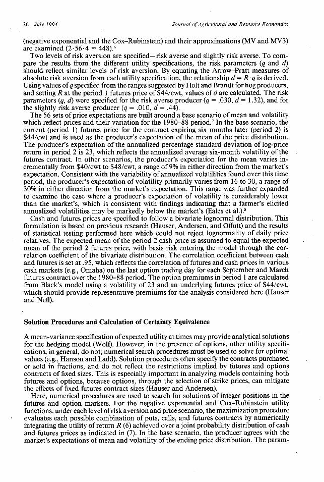
(negative exponential and the Cox-Rubinstein) and their approximations (MV and MV3)are examined (2 56 4 = 448).6

Two levels of risk aversion are specified-risk averse and slightly risk averse. To com-pare the results from the different utility specifications, the risk parameters (q and d)should reflect similar levels of risk aversion. By equating the Arrow-Pratt measures ofabsolute risk aversion from each utility specification, the relationship d = R q is derived.Using values ofq specified from the ranges suggested by Holt and Brandt for hog producers,and setting R at the period 1 futures price of $44/cwt, values of d are calculated. The riskparameters (q, d) were specified for the risk averse producer (q = .030, d = 1.32), and forthe slightly risk averse producer (q = .010, d = .44).

The 56 sets of price expectations are built around a base scenario of mean and volatilitywhich reflect prices and their variation for the 1980-88 period.7 In the base scenario, thecurrent (period 1) futures price for the contract expiring six months later (period 2) is$44/cwt and is used as the producer's expectation of the mean of the price distribution.The producer's expectation of the annualized percentage standard deviation of log-pricereturn in period 2 is 23, which reflects the annualized average six-month volatility of thefutures contract. In other scenarios, the producer's expectation for the mean varies in-crementally from $40/cwt to $48/cwt, a range of 9% in either direction from the market'sexpectation. Consistent with the variability of annualized volatilities found over this timeperiod, the producer's expectation of volatility primarily varies from 16 to 30, a range of30% in either direction from the market's expectation. This range was further expandedto examine the case where a producer's expectation of volatility is considerably lowerthan the market's, which is consistent with findings indicating that a farmer's elicitedannualized volatilities may be markedly below the market's (Eales et al.).8

Cash and futures prices are specified to follow a bivariate lognormal distribution. Thisformulation is based on previous research (Hauser, Andersen, and Offutt) and the resultsof statistical testing performed here which could not reject lognormality of daily pricerelatives. The expected mean of the period 2 cash price is assumed to equal the expectedmean of the period 2 futures price, with basis risk entering the model through the cor-relation coefficient of the bivariate distribution. The correlation coefficient between cashand futures is set at .95, which reflects the correlation of futures and cash prices in variouscash markets (e.g., Omaha) on the last option trading day for each September and Marchfutures contract over the 1980-88 period. The option premiums in period 1 are calculatedfrom Black's model using a volatility of 23 and an underlying futures price of $44/cwt,which should provide representative premiums for the analysis considered here (Hauserand Neff).

Solution Procedures and Calculation of Certainty Equivalence

A mean-variance specification of expected utility at times may provide analytical solutionsfor the hedging model (Wolf). However, in the presence of options, other utility specifi-cations, in general, do not; numerical search procedures must be used to solve for optimalvalues (e.g., Hanson and Ladd). Solution procedures often specify the contracts purchasedor sold in fractions, and do not reflect the restrictions implied by futures and optionscontracts of fixed sizes. This is especially important in analyzing models containing bothfutures and options, because options, through the selection of strike prices, can mitigatethe effects of fixed futures contract sizes (Hauser and Andersen).

Here, numerical procedures are used to search for solutions of integer positions in thefutures and option markets. For the negative exponential and Cox-Rubinstein utilityfunctions, under each level of risk aversion and price scenario, the maximization procedureevaluates each possible combination of puts, calls, and futures contracts by numericallyintegrating the utility of return R (6) achieved over a joint probability distribution of cashand futures prices as indicated in (7). In the base scenario, the producer agrees with themarket's expectations of mean and volatility of the ending price distribution. The param-

36 July 1994


eters of the density function L'(y, f 2) are changed in other scenarios in order to analyzethe choice of marketing strategies as the producer's expectations differ from those of themarket.

For MV and MV3 approximations, the expected utility for each combination of con-tracts is solved by first numerically integrating expressions (8) through (10), below, overthe price distribution in period 2 for each level of risk aversion, so that the mean (m),variance (v), and skewness (s) for each combination of contracts can be determined:

(8) m = E(R) = fJ Rf(y, f 2) dy df2 ,

(9) v = E(R - m)2 = (R - m)2f(y, f 2) dy df2 ,

(10) s = E(R - m)3 = f (R - m)3 f(y, f 2) dy df2 .

Then, using the MV and MV3 specifications (4) and (5), respectively, the expected utilityof each combination of contracts is calculated. 9 For a given set of risk preferences and setof price expectations, the marketing alternative with the highest expected utility is iden-tified as the "best" strategy.

Certainty equivalence (CE) can be used to measure in monetary terms the differencesin expected utility from alternative marketing strategies. CE is the difference between theexpected value and the risk premium (Robison and Barry), and provides monetary valuesof alternative strategies discounted for risk. For a particular risky strategy, the certaintyequivalent is the risk-free return necessary to achieve the same level of expected utilityas that obtained from using the strategy. In the context of a negative exponential utilityfunction, for a given strategy, the expected utility = U = E[-exp(-qR)], where R is arandom variable depending on prices and the market positions associated with the strategy.The certainty equivalent must provide the same level of expected utility, U. As a result,U = E[-exp(-qCE)], which is equal to [-exp(-qCE)] since CE is a particular valuerather than a random variable. Solving for CE, CE = -[ln(-U)]/q. Thus, CE gives amonetary value for the risk-free return that provides the same expected utility as the riskymarket strategy. For the Cox-Rubinstein utility function, CE can be found in a similarmanner and is expressed as CE = [(1 - d)Ul/ (I - '.

Certainty equivalence and the difference in CE are used to calculate the loss from usingthe MV and MV3 procedures to approximate the underlying utility specifications. Considera comparison between the negative exponential and the MV for a particular ending pricescenario. First, the "best" strategy is selected using both the negative exponential speci-fication and the MV. Then, under the negative exponential specification, the CE is cal-culated for the "best" strategy chosen with each procedure. The difference between thetwo CE calculations is defined as the loss in CE from choosing the strategy identified bythe MV framework.

Simulation Results

The use of two utility functions was specified to identify the robustness of the MV approachto a DARA as well as a CARA specification. However, the selected marketing strategiesresulting from the negative exponential and the Cox-Rubinstein functions were identical.Over the range of returns, levels of initial wealth considered, and the degree of risk aversion,the shape of the negative exponential and the Cox-Rubinstein functions were very similar,differing appreciably only at very low levels of wealth (fig. 1). In the appendix, we showthat as the level of wealth increases, the functions more closely approximate each other.Simulations run in the most extreme case, assuming zero initial wealth, did not produceany difference in the findings. The similarity in the results also is likely attributable tothe integer constraints, which do not permit fractions of futures, puts, and call contractsto be utilized. Hence, in this simulation, the MV and the MV3 approximate both theDARA and the CARA specifications to the same degree. Below, because of its use and



Table 1. Best Strategies and CE Loss in $/cwt when Approximations Are Used Rather thanNegative Exponential: Risk Averse Producer

3rd-OrderPrice Neg. Approximation Mean-Variance

Expectations Exponential (MV3) (MV)

Scenario Volatility Mean Best CE Best Loss Best Loss

11121314151617

21222324252627

31323334353637

41424344454647

51525354555657

61626364656667

71727374757677

81828384858687

9999999

16161616161616

19.519.519.519.519.519.519.5

21.2521.2521.2521.2521.2521.2521.25

23232323232323

24.7524.7524.7524.7524.7524.7524.75

26.526.526.526.526.526.526.5

30303030303030

40424344454648

40424344454648

40424344454648

40424344454648

40424344454648

40424344454648

40424344454648

40424344454648

460281

7301,4591,4681,483

46010928

757739

1,4681,472

460352

1,0811,090

850770

1,472

676361364

1,0931,094

8511,499

712607365365

1,0941,0941,580

713689608365

1,3371,0941,823

715689608

1,4181,3371,0941,097

716717

1,4451,4181,4191,4191,341

53.5351.3051.7652.5253.4454.8159.76

51.2147.3546.3946.2447.0748.8554.21

49.4845.2944.2944.1744.8246.1250.83

48.4844.6043.9143.7544.3345.5049.38

47.7044.3143.6643.6544.2145.1848.42

47.3544.3643.8043.6444.1245.0547.87

47.2544.6343.9543.8544.2444.9247.42

47.6845.1744.7644.5344.7745.3547.28

460281

7301,4591,4681,483

46010928

757739

1,4681,472

460352

1,0811,090

850770

1,472

676361364

1,0931,094

8511,499

712607365365

1,0941,0941,580

715689608365

1,3371,0941,836

716689608

1,4181,3371,0942,097

7161,4451,4451,4181,4192,1872,160

.00

.00

.00

.00

.00

.00

.00

.00

.00

.00

.00

.00

.00

.00

.00

.00

.00

.00.00.00.00

.00

.00

.00

.00

.00

.00

.00

.00

.00

.00

.00

.00

.00

.00

.00.00.00.00.00.00

2.43

.00

.00

.00

.00

.00

.002.38

.00

.00

.00

.00

.003.062.29

460281

7301,4591,4681,483

460109

28757739

1,4681,472

460352

1,081847850742

1,471

460361364

1,093850851

1,471

676607365365

1,0941,094

743

679446608365

1,3371,0941,823

680689608

1,4181,3371,0941,095

7161,4451,4451,4181,4181,3371,094

.00

.00

.00

.00

.00.00.00

.00.00.00.00.00.00.00

.00

.00

.00

.03

.00

.21

.21

.03

.00

.00

.00

.06

.00

.62

.25

.00

.00

.00

.00

.00.69

.29

.13

.00

.00

.00

.00

.00

.33

.00

.00

.00

.00

.00

.00

.00

.00

.00

.00

.03.27.77

38 July 1994


Figure 1. Negative exponential (CARA) and Cox-Rubinstein (DARA) utility specifications

familiarity, we focus on differences between the negative exponential utility function andthe MV and MV3 procedures. The only difference between these results and the DARAspecification is that the CE loss from differences in the optimal strategies is modestlylarger with the DARA specification.

Summary results of the simulations are provided in tables 1 and 2. Each row of a tablerepresents an alternative scenario of the ending price distribution. For each price scenario,the strategy selected as "best" under the utility function and approximating approachesis identified.10 The CE is presented for the optimal strategy under the negative exponentialutility specification. The losses (differences) in CE from choosing a strategy using theMV3 and MV approximations when the negative exponential is assumed to be correctalso are identified." For example, for the risk averse producer under scenario 57 (i.e.,expectations of the volatility and mean equal to 23 and 48, respectively), the best strategyis #1,580; with the MV3 approximation, it is also #1,580; and with the MV, it is #743.Calculated using the negative exponential specification, the CE of strategy #1,580 is$48.42/cwt. Because identical strategies are selected, the use of the MV3 approximationresults in no loss. The loss in CE from using the MV approximation is $.69/cwt. Theresults for a slightly risk averse producer are interpreted similarly, with the CE and theloss calculated under the slightly risk averse negative exponential specification.

In general, the results suggest that the approximating procedures work rather well,particularly at or around market expectations and at low levels of volatility. Under marketexpectations (volume = 23, mean = 44), the same strategies are selected by all threespecifications and do not involve options. For the risk averse producer, this strategy is#365, a traditional hedge using a short futures position. For the slightly risk averse pro-ducer, the strategy selected is #1,094, a long cash-only position. Under market expecta-tions, no loss in CE exists by selecting a marketing strategy that considers only mean andvariance. The absence of options in the strategy mix is consistent with Lapan, Moschini,

Notes: The utility specifications are defined in the text. "Volatility" and "Mean" reflect expected annualizedvolatility and mean in $/cwt of the second period price distribution. See text for a discussion of the selectionof "best" strategy and differences in certainty equivalence (CE).

1 10 19 28 37 46 55 64

0.00

-0.50

-1.00

-1.50

-2.00

-2.50

-3.00

-3.50

-4.00

......................... CARA (NegativeExponential)

- DARA (Cox-Rubinstein)

Return ($/cwt)

I I

I


Table 2. Best Strategies and CE Loss in $/cwt when Approximations Are Used Rather thanNegative Exponential: Slightly Risk Averse Producer

PriceExpectation

Scenario Volatility

11 912 913 914 915 916 917 9

21 1622 1623 1624 1625 1626 1627 16

31 19.532 19.533 19.534 19.535 19.536 19.537 19.5

41 21.2542 21.2543 21.2544 21.2545 21.2546 21.2547 21.25

51 2352 2353 2354 2355 2356 2357 23

61 24.7562 24.7563 24.7564 24.7565 24.7566 24.7567 24.75

71 26.572 26.573 26.574 26.575 26.576 26.577 26.5

81 3082 3083 3084 3085 3086 3087 30

3rd-OrderNeg. Approximation Mean-Variance

is Exponential (MV3) (MV)

Mean Best CE Best Loss Best Loss

40424344454648

40424344454648

40424344454648

40424344454648

40424344454648

40424344454648

40424344454648

40424344454648

703281

7301,4591,4681,484

703352

28730

1,4681,4711,485

703379352847742

1,4721,485

703676361

1,093770

1,4721,485

703703607

1,0941,0941,5811,485

703713689

1,3371,0951,8241,485

703716716

1,4181,3381,1071,593

707716720

1,4491,4581,4312,079

53.9651.4351.9852.5253.7755.1661.25

53.1648.0747.1647.1848.4050.8758.62

52.5746.7545.1444.5345.8548.7756.88

52.2446.1744.3443.9545.0747.7155.90

51.8745.6843.9243.7444.7346.8354.85

51.4645.6344.1343.8144.7346.6653.73

51.0245.9644.5244.1344.8846.6753.04

50.4946.9045.8845.5346.1747.6152.76

70328

1730

1,4591,4681,484

703352

28730

1,4681,4711,485

703379352847742

1,4721,485

703676361

1,093770

1,4721,485

703676607

1,0941,0941,4991,485

703713689

1,3371,0951,8241,485

703716689

1,4181,3381,0981,836

707717720

1,4491,4581,4312,079

.00

.00

.00

.00

.00

.00

.00

.00

.00

.00

.00

.00

.00

.00

.00.00.00.00.00.00.00

.00

.00

.00

.00

.00

.00

.00

.00

.01

.00

.00

.00

.01.00

.00

.00

.00

.00

.00

.00

.00

.00

.00

.04

.00

.00

.04

.01

.00

.02

.00.00.00.00.00

70328

1730

1,4591,4681,484

703352

28730

1,4681,4711,485

703379352847742

1,4721,485

703676361

1,093770

1,4721,484

703676607

1,0941,0941,4991,484

703713689

1,3371,0941,8241,484

703716689

1,4181,3381,0981,754

707717720

1,4461,4491,4221,107

.00

.00

.00

.00

.00

.00

.00

.00

.00

.00

.00

.00

.00

.00

.00

.00

.00

.00

.00

.00

.00

.00

.00.00.00.00.00.31

.00

.01

.00

.00

.00

.01

.33

.00

.00

.00

.00.05.00.34

.00

.00

.04

.00

.00

.04

.52

.00

.02

.00

.04

.04

.34

.70

Refer to notes to table 1.


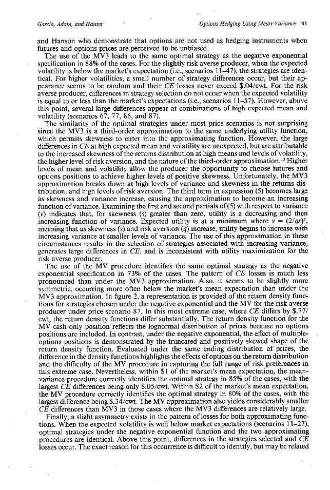
and Hanson who demonstrate that options are not used as hedging instruments whenfutures and options prices are perceived to be unbiased.

The use of the MV3 leads to the same optimal strategy as the negative exponentialspecification in 88% of the cases. For the slightly risk averse producer, when the expectedvolatility is below the market's expectation (i.e., scenarios 11-47), the strategies are iden-tical. For higher volatilities, a small number of strategy differences occur, but their ap-pearance seems to be random and their CE losses never exceed $.04/cwt. For the riskaverse producer, differences in strategy selection do not occur when the expected volatilityis equal to or less than the market's expectations (i.e., scenarios 11-57). However, abovethis point, several large differences appear at combinations of high expected mean andvolatility (scenarios 67, 77, 86, and 87).

The similarity of the optimal strategies under most price scenarios is not surprisingsince the MV3 is a third-order approximation to the same underlying utility function,which permits skewness to enter into the approximating function. However, the largedifferences in CE at high expected mean and volatility are unexpected, but are attributableto the increased skewness of the returns distribution at high means and levels of volatility,the higher level of risk aversion, and the nature of the third-order approximation. 12 Higherlevels of mean and volatility allow the producer the opportunity to choose futures andoptions positions to achieve higher levels of positive skewness. Unfortunately, the MV3approximation breaks down at high levels of variance and skewness in the returns dis-tribution, and high levels of risk aversion. The third term in expression (5) becomes largeas skewness and variance increase, causing the approximation to become an increasingfunction of variance. Examining the first and second partials of(5) with respect to variance(v) indicates that, for skewness (s) greater than zero, utility is a decreasing and thenincreasing function of variance. Expected utility is at a minimum where v = (2/qs)2,meaning that as skewness (s) and risk aversion (q) increase, utility begins to increase withincreasing variance at smaller levels of variance. The use of this approximation in thesecircumstances results in the selection of strategies associated with increasing variance,generates large differences in CE, and is inconsistent with utility maximization for therisk averse producer.

The use of the MV procedure identifies the same optimal strategy as the negativeexponential specification in 73% of the cases. The pattern of CE losses is much lesspronounced than under the MV3 approximation. Also, it seems to be slightly moresymmetric, occurring more often below the market's mean expectation than under theMV3 approximation. In figure 2, a representation is provided of the return density func-tions for strategies chosen under the negative exponential and the MV for the risk averseproducer under price scenario 87. In this most extreme case, where CE differs by $.77/cwt, the return density functions differ substantially. The return density function for theMV cash-only position reflects the lognormal distribution of prices because no optionspositions are included. In contrast, under the negative exponential, the effect of multiple-options positions is demonstrated by the truncated and positively skewed shape of thereturn density function. Evaluated under the same ending distribution of prices, thedifference in the density functions highlights the effects of options on the return distributionand the difficulty of the MV procedure in capturing the full range of risk preferences inthis extreme case. Nevertheless, within $1 of the market's mean expectation, the mean-variance procedure correctly identifies the optimal strategy in 85% of the cases, with thelargest CE differences being only $.05/cwt. Within $2 of the market's mean expectation,the MV procedure correctly identifies the optimal strategy in 80% of the cases, with thelargest difference being $.34/cwt. The MV approximation also yields considerably smallerCE differences than MV3 in those cases where the MV3 differences are relatively large.

Finally, a slight asymmetry exists in the pattern of losses for both approximating func-tions. When the expected volatility is well below market expectations (scenarios 11-27),optimal strategies under the negative exponential function and the two approximatingprocedures are identical. Above this point, differences in the strategies selected and CElosses occur. The exact reason for this occurrence is difficult to identify, but may be related



In

- - Neg. Exp. - #1,341-- MV - #1.094 (cosh-only)

Tc00

I I t

I I

II /

I I I

/ 1/ II

III( I Il~l l

00

3 10 20 30 40 50 60 70 80 90 100

Return ($/cwt)

\

Negative ExponentialStrategy #1,341; p42, c44, c46Expected Value = 52.97Variance = 557.99Skewness = 1.58Kurtosis = 5.56

110 120 130 140 150

Mean-Variance (MV)Strategy #1,094; cash-onlyExpected Value = 48.00Variance = 106.07Skewness = .64Kurtosis = 3.68

Figure 2. Return density functions for optimal strategies chosen under negative exponential andMV utility specifications with expected mean = 48 and expected volatility = 30

to the low variance which implies reduced uncertainty about the returns from alternativestrategies. At extremely low levels of volatility, the mean of the return distribution takeson an increased importance. Selection of the optimal strategy is based more on the expectedutility from higher mean returns. This can be seen clearly in the context of equations (4)and (5). To provide insight into this proposition, additional experiments were performedfor the MV under price scenarios 11-27 assuming risk neutrality (q = 0), which effectivelyeliminates the importance of uncertainty in the decision process. For both risk averse andslightly risk averse producers, the optimal strategies and CE were almost identical tothose identified by the negative exponential and the MV in tables 1 and 2. Hence, at verylow levels of volatility and reduced uncertainty about the return distribution from alter-native strategies, all three specifications identify basically the same strategies which pro-vide the highest mean returns.

E4.

0.001

rf

06

c64

0

6

c500

. . . . . . . . . . . . . . . . . . . . . . . . . . . . . . . . . . . . . . . . . . . . . . . . . . . . . . . . . .

42 July 1994

I . . . . I . i 1 I I . i i 1 I . 1 iIL0 (

i . . , . I . 1 1 1 I . I 1 1 I -I l I-


Summary and Conclusions

The availability of options on agricultural futures has raised some concern about theusefulness of the mean-variance framework in risk-management analyses since optionscan truncate and highly skew the return distributions of marketing strategies. Here, a two-period simulation model of a hog producer's hedging decisions was used to investigatedifferences in optimal strategies and in ex ante utility under alternative utility specificationsin the presence of options and futures contracts. The results from two approximatingprocedures, mean-variance and a third-order Taylor series expansion to a negative ex-ponential function, were contrasted with those generated by the negative exponential utilityfunction (a CARA specification) and the Cox-Rubinstein utility function (a DARA spec-ification). The third-order approximation permits the skewness of the return distributionoften imparted by option positions to influence the selection of the optimal strategy.

Over the simulation values considered here, the marketing strategies selected under theCARA and the DARA specifications were identical. Limited differences in the shape ofthe utility functions existed except at very low levels of wealth. The similarity in theresults also may be attributable to the integer marketing constraints which do not permitfractions of futures, put, or call contracts to be used.

The findings suggest that the third-order approximation and the mean-variance frame-work provide rather good approximations, particularly at or around market expectations.Overall, both approximating procedures accurately identify optimal strategies in a highpercentage of cases. When errors occur, often the magnitude of the CE differences is smallon a $/cwt basis, except for the third-order approximation, which is particularly sensitiveto positive skewness at higher levels of risk aversion and volatility. While the third-orderapproximation is the most accurate at identifying the optimal strategies, the performanceof the mean-variance formulation also is attractive, particularly in light of its ease ofunderstanding and use, and because it is less susceptible to the large errors encounteredin the MV3 formulation.

In addition, the results suggest that when producers have low volatility expectationsrelative to the market, the MV3 and MV formulations also work well. For the risk averseand slightly risk averse producers, appropriate strategies are identified in most cases whenvolatility expectations were below the market's. This indicates that if a producer's volatilityexpectations are low relative to the market, as some research has suggested, then the useof these approximations may identify utility maximizing strategies in a consistent manner.

In general, the results regarding the usefulness of the mean-variance framework in thepresence of options are consistent with those of Hanson and Ladd who examined thisquestion in a more simplified framework which assumed continuous (non-discrete) po-sitions in only futures and a put option with a single strike price, normally distributedoutput price, no transactions costs, and no basis uncertainty. The findings from oursimulation, which considers discrete contracts, basis risk, lognormality in prices, trans-actions costs, and alternative utility specifications, do not change the general conclusionthat the mean-variance criterion is a good evaluation tool.

[Received March 1992;final revision received December 1993.]

Notes

The use of the expected utility framework to analyze decision making in a risky environment has beencriticized (Machina). Similarly, it is possible to generate examples where a mean-variance analysis leads toresults which are inconsistent with expected utility theory. Nevertheless, the use of expected utility and mean-variance in theoretical and applied decision making suggests the importance of our analysis.

2 To make the empirical analysis manageable, the number of strike prices for puts and calls and the numberof contracts and options are limited. This is discussed below in the empirical specification section.

3 Our findings suggest that with larger production units, and less likelihood of the substitution of options forfutures, MV also may work well.



4 Margin requirements are not explicitly considered here since they can be satisfied by pledging U.S. TreasuryBills. Also, margin calls are not explicitly considered in the structure of the model.

5 Examination of situations where multiple futures contracts or multiple options contracts at the same strikeprice were most likely to occur (i.e., where producer expectations of price mean and volatility differ most fromthe market) indicated that these one-contract restrictions were not binding.

6 Examination of tables 1 and 2 may facilitate an understanding of the structure of the simulations. Thesetables provide results for the negative exponential, MV, and the MV3 specifications for the risk averse andslightly risk averse producers under the 56 price scenarios. Similar calculations for the Cox-Rubinstein speci-fication were made, but, as discussed later, were not presented.

7 Daily closing futures prices from the Chicago Mercantile Exchange and daily high and low prices fromInterior Iowa, Omaha, and Sioux City livestock markets were provided by G. Futrell and D. O'Brien, Departmentof Economics, Iowa State University.

8 For the period 1983-87, errors in the futures price forecasts of the price at contract expiration six monthslater ranged from $.04/cwt to $18.99/cwt, with an average error of $5.66/cwt. For the period 1980-88, theannualized volatilities of the hog futures closing prices ranged from 16 to 30. Eales et al. found that soybeanproducers had annualized volatility expectations of prices as low as 9.45, even when the market's impliedvolatility was 22.

9 The double integrals in equations (7)-(10) are computed using Gaussian adaptive composite quadrature.Gaussian quadrature is performed by choosing Ncash and Nfutures prices to interpolate the continuous integrand.To complete the inner integral, R is calculated for each cash price, given the set of futures prices. These valuesof R are multiplied by the joint density function evaluated at the combinations of cash and future prices usedto calculate R. These values are in turn multiplied by standard quadrature interpolating values (weights) whichdepend on the order of integration and are taken from tables. To increase precision, composite quadraturedivides the intervals LF2 to UF2 and LY to UY into several subintervals. Adaptive quadrature adapts the lengthof each of these subintervals to increase the precision where the function changes most rapidly. For furtherdiscussion, see Conte and de Boor. The GAUSS computer programs used are available from the authors. Analternative procedure to optimize (7) involves iterating between a numerical integration routine and a nonlinearoptimization routine (Kaylen, Preckel, and Loehman). This approach permits non-integer solutions, ignoringmarketing constraints, and removes part of the attractiveness of options positions which can be used to achieveintermediate trading positions (Hauser and Andersen).

'0 A description of the "best" strategies is omitted for brevity, but is available from the authors upon request."In several cases, the optimal strategies were different, but the loss in CE was less than 1 ¢ per cwt.12 The skewness of the returns distribution under the negative exponential function for scenarios 67, 77, 86,

and 87 are .53, 1.04, 1.92, and 1.58, respectively.

References

Black, F. "The Pricing of Commodity Contracts." J. Financ. Econ. 3(1976): 167-79.Conte, S. D., and C. de Boor. Elementary Numerical Analysis: An Algorithmic Approach, 3rd ed. New York:

McGraw-Hill Book Co., 1980.Cox, J. C., and M. Rubinstein. Options Markets. Englewood Cliffs NJ: Prentice-Hall, Inc., 1985.Eales, J. S., B. K. Engel, R. J. Hauser, and S. R. Thompson. "Grain Price Expectations of Illinois Farmers and

Grain Merchandisers." Amer. J. Agr. Econ. 72(1990):701-08.Hanson, S. D., and G. W. Ladd. "Robustness of the Mean-Variance Model with Truncated Probability Distri-

butions." Amer. J. Agr. Econ. 73(1991):436-45.Hauser, R. J., and D. K. Andersen. "Hedging with Options under Variance Uncertainty: An Illustration of

Pricing New-Crop Soybeans." Amer. J. Agr. Econ. 69(1987):38-45.Hauser, R. J., D. K. Andersen, and S. E. Offutt. "Pricing Options in Hog and Soybean Futures." In Proceedings

of the NC-134 Conference on Applied Commodity Price Analysis, Forecasting, and Risk Management, pp.23-39. NCR-134 Regional Research Committee, Iowa State University, Ames, 1984.

Hauser, R. J., and D. L. Neff. "Pricing Options on Agricultural Futures: Departures from Traditional Theory."J. Futures Mkts. 5(1985):539-77.

Holt, M., and J. Brandt. "Combining Price Forecasting with Hedging of Hogs: An Evaluation Using AlternativeMeasures of Risk." J. Futures Mkts. 5(1985):297-309.

Kaylen, M. S., P. V. Preckel, and E. T. Loehman. "Risk Modeling via Direct Utility Maximization UsingNumerical Quadrature." Amer. J. Agr. Econ. 69(1987):701-06.

Kroll, Y., H. Levy, and H. M. Markowitz. "Mean-Variance Versus Direct Utility Maximization." J. Finance34(1984):47-61.

Lapan, H., G. Moschini, and S. D. Hanson. "Production, Hedging, and Speculative Decisions with Options andFutures Markets." Amer. J. Agr. Econ. 73(1991):66-74.

Machina, M. J. "Choice Under Uncertainty: Problems Solved and Unsolved." Econ. Perspectives 1(1987):121-54.

Meyer, J. "Two-Moment Decision Models and Expected Utility Maximization." Amer. Econ. Rev. 77(1987):421-30.

44 July 1994

Garcia, Adam, and Hauser Options Hedging Using Mean- Variance 45

Robison, L. J., and P. J. Barry. The Competitive Firm's Response to Risk. New York: Macmillan PublishingCo., 1987.

Wolf, A. "Optimal Hedging with Futures Options." J. Econ. and Bus. 39(1987):141-58.

Appendix

The Cox-Rubinstein (DARA) function is more likely to produce different rankings than the negative exponential(CARA) function when the initial wealth is small. To verify this, we show that the relative percentage differencein utility between the two functions resulting from incremental changes in wealth is very large when initialwealth is small, but is small when initial wealth is large.

Let U1 = -exp(-qR), the CARA function, and U2 = (1/(1 - d))Rl -d, the DARA function, where the termsare defined in the text. Then,

dU1d = qexp(-qR), anddR

dU2 = Rd

dR

Expressing changes in utility as percentage changes resulting from incremental changes in R leads to

dU, qexp(-qR)dR-- ~ = = -qdR, and

U, -exp(-qR)

dU2 R-ddR (1 - d)dRU2 (1/(1 - d))R -d R

The relative percentage change in utility between U2 and Ul for incremental changes in wealth can then beexpressed as

dU2 (1 - d)dRU2 R

dU -qdR

Ui

which after normalizing to make the risk aversion coefficients comparable, d = R q (see text), can be written as

dU2 (1 - d)dR

U2 R -(1 - qR)dR

dU, -qdR qR

U.

As R gets smaller,

lim (1 - qR)dRlim = co,R-.O

+ qR

the relative difference between the two functions gets larger for smaller R. However, as R gets larger,

lim -(1 qR)dR lim - = 1 (by L'Hopital's Rule).R-, qR R-oo q

Hence, as R gets larger, the difference between the two functions approaches a positive finite constant, showingthat differences between the two functions will be largest for small values of R.

Documents

The Use of Mean-Variance for Commodity Futures and Options … · Options Hedging Using Mean- Variance 33 only their integer multiples. A much larger set of possible (simultaneous)