THE USE OF PAMS DATA TO EVALUATE REGIONAL EMISSION · PDF fileTami L. Haste-Funk Lyle R. Chinkin ... The u se of PAMS data to evaluate regional emission inventories in California

ANALYSIS OF PAMS DATA IN CALIFORNIAVOLUME II: THE USE OF PAMS DATA TO

EVALUATE REGIONAL EMISSIONINVENTORIES IN CALIFORNIA

FINAL REPORTSTI-998392-1884-FR

By:Tami L. Haste-Funk

Lyle R. ChinkinSonoma Technology, Inc.

Petaluma, CA

Prepared for:California Air Resources Board

Sacramento, CA

May 1999

ANALYSIS OF PAMS DATA IN CALIFORNIAVOLUME II: USE OF PAMS DATA TO

EVALUATE REGIONAL EMISSIONINVENTORIES IN CALIFORNIA

FINAL REPORTSTI-998392-1884-FR

By:Tami L. Haste-Funk

Lyle R. ChinkinSonoma Technology, Inc.

1360 Redwood Way, Suite CPetaluma, CA 94954-1169

Prepared for:California Air Resources Board

2020 L. StreetSacramento, CA 95814

May 26, 1999

[BLANK PAGE]

iii

PREFACE

In accordance with the 1990 Clean Air Act Amendments, the U.S. EnvironmentalProtection Agency (EPA) initiated the Photochemical Assessment Monitoring Stations (PAMS)program for serious, severe, and extreme ozone nonattainment areas. The PAMS networksmonitor for volatile organic compounds (VOCs), ozone, oxides of nitrogen (NOx), andmeteorological parameters. The PAMS networks were designed to provide data for theassessment of population exposure, ozone formation, and evaluation of ozone controlstrategies. The EPA Office of Air Quality Planning and Standards has sought to provide theEPA regional offices and the states with the necessary analytical tools, training, and guidanceto collect and use the PAMS data. To this end, the EPA, California Air Resources Board(ARB), Sacramento Metropolitan Air Quality Management District, San Joaquin ValleyUnified Air Pollution Control District, and Ventura County Air Pollution Control Districtsponsored research into the analysis of PAMS air quality and meteorological data collected atthe Districts’ PAMS sites in Sacramento, Fresno, and Ventura counties and the ARB's long-term trend sites located in Los Angeles and San Diego. Requested tasks encompass upper-airmeteorological data processing and analyses, emission inventory evaluation, and trendsanalyses. Results of the data analyses for these three topic areas are presented in threevolumes:

Analysis of PAMS Data in California Volume I: The use of PAMS radar profiler and RASSdata to understand the meteorological processes that influence air quality in selectedregions of California. MacDonald C.P., Chinkin L.R., Dye T.S., Anderson C.B.(1999) Report prepared for the U.S. Environmental Protection Agency, ResearchTriangle Park, NC by Sonoma Technology, Inc., Petaluma, CA, STI-998391-1888-FR,May.

Analysis of PAMS Data in California Volume II: The use of PAMS data to evaluate regionalemission inventories in California. Haste-Funk T.L., Chinkin L.R. (1999) Reportprepared for the U.S. Environmental Protection Agency, Research Triangle Park, NCby Sonoma Technology, Inc., Petaluma, CA, STI-998392-1884-FR, May.

Analysis of PAMS Data in California Volume III: Trends analyses of California PAMS andlong-term trend air quality data (1987-1997). Wittig A.E., Main H.H., Roberts P.T.,Hurwitt S.H. (1999) Report prepared for the U.S. Environmental Protection Agency,Research Triangle Park, NC by Sonoma Technology, Inc., Petaluma, CA, STI-998393-1885-FR, May.

iv

v

ACKNOWLEDGMENTS

The authors of this report would like to thank Mark Schmidt for coordinating this workeffort for the EPA, and Sacramento Metropolitan Air Quality Management District staff, SanJoaquin Valley Unified Air Pollution Control District staff, and Ventura County Air PollutionControl District staff, and Don Hammond of the ARB. We would also like to thank JanaSchwartz, Martina Shultz, and Sandy Smethurst of STI for preparation of the text and figurespublished in the report.

[BLANK PAGE]

vii

TABLE OF CONTENTS

Section Page

PREFACE .....................................................................................................iiiACKNOWLEDGMENTS....................................................................................vLIST OF FIGURES .......................................................................................... ixLIST OF TABLES ......................................................................................... xiii

1. INTRODUCTION ..................................................................................... 1-11.1 BACKGROUND ................................................................................ 1-11.2 OVERVIEW OF THE REPORT............................................................. 1-2

2. TECHNICAL APPROACH USED AND UNCERAINTY ISSUES FOR EMISSIONINVENTORY EVALUATIONS .................................................................... 2-12.1 TECHNICAL APPROACH................................................................... 2-12.2 UNCERTAINTY ISSUES..................................................................... 2-2

3. AMBIENT AND EMISSION INVENTORY DATA............................................ 3-13.1 AMBIENT DATA .............................................................................. 3-1

3.1.1 Ambient Meteorological Data....................................................... 3-13.1.2 Ambient Air Quality Data ........................................................... 3-13.1.3 Spatial Variability and Characteristics of Ambient Data ....................... 3-3

3.2 EMISSION INVENTORY DATA ........................................................... 3-3

4. EMISSION INVENTORY EVALUATION ...................................................... 4-14.1 HYDROCARBON/NOx AND CO/NOx RATIO ANALYSES .......................... 4-1

4.1.1 Weekday Hydrocarbon/NOx Ratio Analyses ..................................... 4-14.1.2 Weekday CO/NOx Ratio Analyses ................................................. 4-24.1.3 Potential Effects of Ambient Background Pollutant Concentrations ......... 4-34.1.4 Weekday Versus Weekend Hydrocarbon/NOx and CO/NOx Ratio

Comparison ............................................................................ 4-44.2 DETAILED HYDROCARBON COMPOSITION ANALYSES........................ 4-5

4.2.1 Major Groups of Organic Compounds ............................................ 4-54.2.2 Detailed Hydrocarbon Composition – All Source Categories ................. 4-64.2.3 Detailed Hydrocarbon Composition – Area, Mobile, and Point Sources ... 4-94.2.4 Hydrocarbon Maximum Incremental Reactivity................................4-13

5. CONCLUSIONS FROM THE EMISSION INVENTORY EVALUATION ANDRECOMMENDATIONS ............................................................................. 5-15.1 CONCLUSIONS – HYDROCARBON/NOx AND CO/NOx RATIO

ANALYSES...................................................................................... 5-15.2 CONCLUSIONS – HYDROCARBON SPECIES ANALYSES ........................ 5-35.3 RECOMMENDATIONS ...................................................................... 5-4

viii

TABLE OF CONTENTS (Concluded)

Section Page

6. REFERENCES ......................................................................................... 6-1

APPENDIX A: HYDROCARBON SPECIES MEASURED AT CLOVIS, FRESNO,DEL PASO, FOLSOM, EL RIO, AND SIMI VALLEY DURINGTHE SUMMER OF 1996 ............................................................A-1

ix

LIST OF FIGURES

Figure Page

1-1. Map of California and the PAMS ambient monitoring site locations in Sacramento,Fresno, and Ventura counties ................................................................... 1-3

2-1. Wind quadrant definitions surrounding an ambient monitor ............................... 2-3

3-1. Frequency distribution of wind direction by quadrant for weekday data collectedfrom 0500-0800 PST during the summer of 1996 in Fresno(Clovis and Fresno), Sacramento (Del Paso and Folsom), and Ventura(El Rio and Simi Valley) counties .............................................................. 3-5

3-2. Annotated box-whisker plot...................................................................... 3-5

3-3. Box-whisker statistical plots of ambient a) TNMOC, b) NOx, andc) CO concentrations at each site for all valid weekday samples collectedat 0500-0800 PST during the summer of 1996 ............................................... 3-6

3-4. Source category contributions to ROG, NOx, and CO for a) Fresno, b) Sacramento,and c) Ventura counties as reported in the weekday county-wide emissioninventory provided by the ARB................................................................. 3-7

4-1. Weekday average ambient and average county total emission inventory (EI)hydrocarbon/NOx ratios in a) Fresno, b) Sacramento, and c) Ventura countiesfrom 0500-0800 PST.............................................................................4-15

4-2. Weekday average ambient and average county total emission inventory (EI)CO/NOx ratios in a) Fresno, b) Sacramento, and c) Ventura countiesfrom 0500-0800 PST.............................................................................4-16

4-3. Average ambient and average county total emission inventory (EI) weekdayand Saturday hydrocarbon/NOx ratios at a) Clovis and b) Fresnofrom 0500-0800 PST.............................................................................4-17

4-4. Average ambient and Sacramento County total emission inventory (EI) weekdayand Saturday hydrocarbon/NOx ratios at Del Paso from 0500-0800 PST ..............4-18

4-5. Average ambient and average county total emission inventory (EI) weekday andSaturday CO/NOx ratios at a) Clovis and b) Fresno from 0500-0800 PST.............4-19

4-6. Average ambient and Sacramento County total emission inventory (EI) weekdayand Saturday CO/NOx ratios at Del Paso from 0500-0800 PST..........................4-20

x

LIST OF FIGURES (Continued)

Figure Page

4-7. Average ambient weekday and average county total emission inventory (EI)paraffin, olefin, and aromatic species group composition for a) Fresno,b) Sacramento, and c) Ventura from 0500-0800 PST......................................4-21

4-8. Comparison of the 0500-0800 PST weekday average ambient and averageemission inventory chemical species composition for area, point, and mobilesources combined for the Clovis and Fresno PAMS sites and the Fresno Countyemission inventory ...............................................................................4-22

4-9. Comparison of the 0500-0800 PST weekday average ambient and averageemission inventory chemical species composition for area, point, and mobilesources combined for the Del Paso and Folsom PAMS sites and the SacramentoCounty emission inventory......................................................................4-23

4-10. Comparison of the 0500-0800 PST weekday average ambient and averageemission inventory chemical species composition for area, point, and mobilesources combined for the El Rio and Simi Valley PAMS sites and the VenturaCounty emission inventory......................................................................4-24

4-11. Comparison of the 0500-0800 PST average ambient and average emissioninventory chemical species composition for the Clovis and Fresno PAMS sitesand the area source component of the Fresno County emission inventory .............4-25

4-12. Comparison of the 0500-0800 PST average ambient and average emissioninventory chemical species composition for the Clovis and Fresno PAMS sitesand the mobile source component of the Fresno County emission inventory ..........4-26

4-13. Comparison of the 0500-0800 PST average ambient and average emissioninventory chemical species composition for the Clovis and Fresno PAMS sitesand the point source component of the Fresno County emission inventory ............4-27

4-14. Comparison of the 0500-0800 PST average ambient and average emissioninventory chemical species composition for the Del Paso and Folsom PAMS sitesand the area source component of the Sacramento County emission inventory .......4-28

4-15. Comparison of the 0500-0800 PST average ambient and average emissioninventory chemical species composition for the Del Paso and Folsom PAMS sitesand the mobile source component of the Sacramento County emission inventory ....4-29

xi

LIST OF FIGURES (Concluded)

Figure Page

4-16. Comparison of the 0500-0800 PST average ambient and average emissioninventory chemical species composition for the Del Paso and Folsom PAMS sitesand the point source component of the Sacramento County emission inventory ......4-30

4-17. Comparison of the 0500-0800 PST average ambient and average emissioninventory chemical species composition for the El Rio and Simi Valley PAMSsites and the area component of the Ventura County emission inventory ..............4-31

4-18. Comparison of the 0500-0800 PST average ambient and average emissioninventory chemical species composition for the El Rio and Simi Valley PAMS sitesand the mobile source component of the Ventura County emission inventory.........4-32

4-19. Comparison of the 0500-0800 PST average ambient and average emissioninventory chemical species composition for the El Rio and Simi Valley PAMSsites and the point source component of the Ventura County emission inventory.....4-33

4-20. Comparison of the 0500-0800 PST average ambient- and average emissioninventory-derived relative reactivity of chemical species (area, point, andmobile sources combined) for the Clovis and Fresno PAMS sites and theFresno County emission inventory ............................................................4-34

4-21. Comparison of the 0500-0800 PST average ambient- and average emissioninventory-derived relative reactivity of chemical species (area, point, andmobile sources combined) for the Del Paso and Folsom PAMS sites and theSacramento County emission inventory ......................................................4-35

4-22. Comparison of the 0500-0800 PST average ambient- and average emissioninventory-derived relative reactivity of chemical species (area, point, and mobilesources combined) for the El Rio and Simi Valley PAMS sites and the VenturaCounty emission inventory......................................................................4-36

[BLANK PAGE]

xiii

LIST OF TABLES

Table Page

3-1. Summary of the weekday ambient average TNMOC, identified NMOC, NOx,and CO data meeting all validity and screening criteria at Fresno, Clovis,Del Paso, Folsom, El Rio, and Simi Valley .................................................. 3-8

4-1. Average ambient- and emission inventory-derived hydrocarbon/NOx ratios for theambient weekday data collected from 0500-0800 PST during the summer of 1996 and0500-0800 PST county total emission inventory data at Fresno, Sacramento, andVentura counties ..................................................................................4-37

4-2. Ratios of the ambient- and emission inventory-derived weekdayhydrocarbon/NOx ratios in Fresno, Sacramento, and Ventura counties.................4-37

4-3. Average ambient- and emission inventory-derived weekday CO/NOx ratios forthe ambient data collected from 0500-0800 PST during the summer of 1996 and0500-0800 PST county total emission inventory data at Fresno, Sacramento,and Ventura Counti...............................................................................4-38

4-4. Ratios of the ambient- and emission inventory-derived weekday CO/NOx ratiosin Fresno, Sacramento, and Ventura counties ...............................................4-38

4-5a. Average ambient- and emission inventory-derived hydrocarbon/NOx ratios forthe ambient weekday data collected from 0500-0800 PST during the summerof 1996 accounting for background concentrations and 0500-0800 PST countytotal emission inventory data at Fresno, Sacramento, and Ventura counties...........4-39

4-5b. Average ambient- and emission inventory-derived CO/NOx ratios for theambient weekday data collected from 0500-0800 PST during the summerof 1996 accounting for background concentrations and 0500-0800 PST countytotal emission inventory data at Fresno, Sacramento, and Ventura counties...........4-40

4-6. Summary of the Saturday ambient average TNMOC, NOx, and CO data meetingall validity and screening criteria at Fresno, Clovis, and Del Paso Manor.............4-41

4-7. Average ambient- and emission inventory-derived Saturday hydrocarbon/NOx ratiosfor the ambient data collected from 0500-0800 PST during the summer of 1996and 0500-0800 PST county total emission inventory data for Fresno andSacramento counties..............................................................................4-41

4-8. Ratios of the ambient- and emission inventory-derived Saturdayhydrocarbon/NOx ratios in Fresno and Sacramento counties .............................4-42

xiv

LIST OF TABLES (Concluded)

Table Page

4-9. Average ambient- and emission inventory-derived Saturday CO/NOx ratiosfor the ambient data collected from 0500-0800 PST during the summer of 1996and 0500-0800 PST county total emission inventory data for Fresno andSacramento counties..............................................................................4-42

4-10. Ratios of the ambient- and emission inventory-derived Saturday CO/NOx ratiosin Fresno and Sacramento counties............................................................4-43

1-1

1. INTRODUCTION

1.1 BACKGROUND

Emission inventory development is a complex process that involves estimating andcompiling emissions activity data from hundreds of point, area, and mobile sources in a givenregion. Because of the complexities involved in developing emission inventories, and theimplications of errors in the inventory on air quality model performance and control strategyassessment, it is important to evaluate the accuracy and representativeness of any inventorythat is intended for use in pollution control strategy assessment. One way to assess a regionalemission inventory is to perform a top-down inventory evaluation by comparing ozoneprecursor emission estimates to ambient air quality data using ratio comparisons ofhydrocarbon/NOx and CO/NOx (Haste et al, 1998a, b; Korc et al, 1993, 1995; Fujita et al.,1992, 1994). Comparison of ambient data and emission inventory estimates are useful forexamining the relative mass and composition of the ambient air and emissions estimates.

The objective of this work effort is to assess the consistency of the most recentlyestimated regional emission inventory for three counties in California (e.g., Fresno,Sacramento, and Ventura counties) with ambient data. Ambient hydrocarbon, CO, and NOx

measurements collected during the summer of 1996 at six Photochemical AssessmentMonitoring Stations (PAMS) located in Fresno, Sacramento, and Ventura counties werecompared to 1996 county-wide emission estimates of hydrocarbon, CO, and NOx. The 1996ambient data were selected for this analysis to correspond to the most recent and readilyavailable inventory for these counties. Figure 1-1 depicts the State of California as well as thelocation of the PAMS monitoring sites in each of the three counties studied.

Comparisons of ambient data and emission estimates for hydrocarbon, CO, and NOx

are based on the premise that ambient concentrations are primarily influenced by freshemissions emitted in the vicinity of the monitor. However, precursor transport, carryovereffects, and chemical reactions can also influence ambient concentrations. The influence ofthese confounding effects on the comparison can be minimized (but not eliminated) by selectingmonitoring sites located in areas with high emission rates, and by examining data collectedwhen emission rates are high and reaction rates are low. Early morning sampling periods arethe most appropriate to use when making emission comparisons because typically emissions arehigh, while wind speed, atmospheric mixing height, temperature, and chemical reactivity arelow. Data from early morning sampling periods are most likely to contain minimal effectsfrom upwind transport and photochemistry.

Comparisons of ambient data and emission estimates for hydrocarbon and NOx are alsobased on the assumption that emission inventory NOx estimates are more accurate thanhydrocarbon estimates. Since NOx emissions are directly associated with combustion sources(primarily point and mobile sources) and hydrocarbons are emitted by a much broader range ofsources (both man-made and biogenic, as well as combustion and non-combustion processes),it is assumed that NOx is more accurately estimated in emission inventories. Past studiessuggest that NOx emission estimates are fairly accurate, while hydrocarbon emission estimatesare more uncertain (ARB, 1997; Gertler and Pierson, 1996).

1-2

1.2 OVERVIEW OF THE REPORT

This report consists of six sections. Section 2 provides a discussion of the technicalapproach and the uncertainty issues associated with top-down emission inventory evaluations.Section 3 describes the characteristics of the ambient air quality, meteorological, and emissioninventory data used in the evaluation. Section 4 provides an analysis of the emission inventoryincluding hydrocarbon/NOx and CO/NOx ratio analyses and detailed hydrocarbon composition.Section 5 includes a summary of results, conclusions, and recommendations on possibleimprovements to the inventory. Section 6 contains the report references. A list ofhydrocarbon species measured at each monitoring site used in this study is provided inAppendix A.

1-3

Figure 1-1. Map of California and the PAMS ambient monitoring site locationsin Sacramento, Fresno, and Ventura counties.

Folsom

Del Paso Manor

Clovis

Fresno - 1st Street

El Rio

Simi Valley

Sacramento County

Fresno County

Ventura County

[BLANK PAGE]

2-1

2. TECHNICAL APPROACH USED AND UNCERTAINTY ISSUES FOREMISSION INVENTORY EVALUATIONS

2.1 TECHNICAL APPROACH

Top-down emission inventory evaluations can be divided into two parts: 1) comparisonof ambient- and emission inventory-derived hydrocarbon/NOx and CO/NOx ratios, and2) comparison of chemical species groups and/or individual chemical species. Comparison ofambient- and emission inventory-derived hydrocarbon/NOx and CO/NOx ratios provides amethod to compare the relative mass of pollutants in the ambient air and in the inventory.Because certain species are characteristic of emissions from specific source categories,comparisons of the species in the ambient air and in the emission inventory can serve as anindicator of the representativeness of the inventory.

In this study, comparisons between weekday ambient-derived ratios and emissioninventory-derived hydrocarbon/NOx and CO/NOx ratios were calculated for each of the fourwind quadrants surrounding the ambient monitor at each site and were compared to the countytotal emissions ratios. Figure 2-1 depicts the spatial designation of the four wind quadrantssurrounding an ambient monitor. Typically, analyses are performed by spatially matching agridded, speciated, temporally resolved (hourly) emission inventory to the geographicalposition of the ambient monitoring site and the four wind quadrants surrounding the site.Detailed spatial analyses could not be made in this study, however, because the emissioninventory data were resolved only to the county level. Instead, wind pattern analyses wereconducted to determine the transport distances air parcels traveled during the morning ambientsampling period. Because of the various meteorological factors that could affect ambientpollutant ratios, ambient-derived ratios are presented for all four quadrants.

Data collected during the 0500-0800 PST sampling period were used for the analysis tocapture a time period when fresh emissions are generally high, while temperature and chemicalreactivity are low. It should be recognized that CO and NOx emissions from point sourceswith elevated stacks may be injected above the morning inversion and, hence, may notcontribute to surface-level concentrations. In order to examine the effects of elevated pointsource emissions, comparisons were made both including and excluding emissions from pointsources.

Speciation profiles provide a detailed breakdown of the individual chemical speciesemitted by a specific source category. When an emission inventory is “speciated” each sourcecategory is assigned a speciation profile which is then used to disaggregate total hydrocarbonemissions into individual chemical compounds. Comparisons of the individual hydrocarbonspecies in the ambient air and in the inventory can provide insight into how well the speciationprofiles used to disaggregate the emission inventory represent the chemical composition of theambient air. Comparisons of the relative amounts of individual organic hydrocarbon speciesand species groups in the ambient data and in the inventory were made to evaluate the accuracyof the inventory speciation. Comparisons of the emissions from point, area, and on-roadmobile sources were performed to evaluate how well the emissions from each source categorycompare with the ambient data.

2-2

2.2 UNCERTAINTY ISSUES

The uncertainties associated with comparisons of emission inventory-derived andambient-derived hydrocarbon/NOx and CO/NOx ratios can be divided into three categories:(1) accuracy of the emission inventory, (2) accuracy of the measurements of ambientconcentrations, and (3) suitability of comparisons. Issues that must be accounted for are listedbelow.

• Emission inventory-related issues such as spatial and temporal allocation, speciationprofiles, and assignment of the correct profiles to source categories.

• Measurement-related issues such as data quality and validation including the influenceof instrument detection limits and precision; the identification, misidentification, or lackof identification of species; potential sampling or handling losses of total mass orindividual species; and the overall uncertainties of the ambient measurements.

• Comparison-related issues such as the matching of hydrocarbon species in the emissioninventory and ambient hydrocarbon species; the temporal matching of the emissions andambient data; and meteorological factors such as inversion height, wind speed, andwind direction which influence which emissions are sampled in the ambient air.

• Effect of background concentrations; fresh emissions are not the only influence onmonitoring data.

• Meteorological effects; emissions injected above the morning inversion layer may notbe detected at a ground level monitor.

Uncertainties associated with the emission inventory are inherent in the methodologyused to develop the inventory. Emissions estimates are only as accurate as the underlyingactivity data and emission factors used to calculate the estimates. Emission inventoryevaluations are typically performed on emissions data that are intended for use in air qualitymodeling, and therefore should be of the highest possible quality. Measurement-relateduncertainties in the ambient data are minimized by using ambient data that have undergoneexhaustive quality assurance/quality control (QA/QC) protocols and screening criteria.Comparison-related issues are addressed by matching individual chemical species in theambient data and the inventory prior to analysis. Emissions and ambient data are compared forthe same early-morning time period and are typically matched spatially by wind speed anddirection.

In this study, the spatial matching of emissions and ambient data introduces a degree ofuncertainty. Because the emissions data are resolved only at the county level, the county-totalemissions were compared to the average of the ambient data samples, rather than to theindividual quadrants’ concentration ratios. In regions where ambient concentrations are fairlyuniform, the county-total emissions comparison is more robust. However, in regionsexhibiting high ambient concentration gradients, it is likely that a county-total emissioninventory is not adequately resolved to make sound comparisons between the ambient data andthe inventory.

2-3

Wind Quadrant 1(0-90°)




S

EW

N 0°

270°

180°

90°

AmbientMonitor

Figure 2-1. Wind quadrant definitions surrounding an ambient monitor. The quadrantsrepresent the direction from which the wind is blowing.

[BLANK PAGE]

3-1

3. AMBIENT AND EMISSION INVENTORY DATA

3.1 AMBIENT DATA

The ambient data used to evaluate the emission inventory for Sacramento, Fresno, andVentura counties consisted of early morning weekday and Saturday surface meteorological dataand surface concentrations of hydrocarbon, CO, and NOx collected at six PAMS monitoringsites during the summer of 1996. Ambient air quality data from two sites in each county wereacquired: Del Paso and Folsom in Sacramento; Clovis and Fresno in Fresno County; and ElRio and Simi in Ventura County. Monitoring sites were selected based on geographic locationand diversity of emission source influences as well as the availability and quality of ambientdata. Three-hour average hydrocarbon samples were collected at each site during the0500-0800 PST period every six days from July through September 1996. Hourly CO andNOx data were collected for the same time period at each site except at the Folsom site whereCO was not measured.

3.1.1 Ambient Meteorological Data

Wind analyses were performed to determine air parcel travel distances for the0500-0800 PST time period, corresponding to the air quality data collected from July throughSeptember 1996. To determine the 0500-0800 PST transport of surface emissions, vectoraverage winds were calculated at each site. Frequency distributions of 0500-0800 PST averagewind directions by quadrant for each site are shown in Figure 3-1.

From 0500-0800 PST, surface winds are predominately from the southeast in FresnoCounty (Clovis and Fresno) and Sacramento County (Del Paso and Folsom). In VenturaCounty at El Rio, early-morning winds are predominately from the northeast whileearly-morning winds at Simi Valley are typically from the south. Average transport distancesfor the 0500-0800 PST time period were calculated for each site. Three-hour transportdistances in Fresno and Sacramento counties were approximately 13 km. The averagetransport distance in Ventura County is slightly higher, ranging from 15 to 20 km.

The wind summary presented above is useful for investigating the directional influenceon the ambient monitor as well as how far emissions may have traveled to the monitor duringthe early morning. The wind summaries can also be used for comparing pollutant ratios in theambient data to the emission inventory ratios for the spatial configurations corresponding to thefour wind quadrants if a gridded emission inventory is available. However, because theinventory data used in this evaluation are resolved at the county level, a comparison betweenthem and the ambient data by wind quadrant should not be made.

3.1.2 Ambient Air Quality Data

During the summer of 1996, hourly CO and NOx data were collected at Clovis, Fresno,Del Paso, El Rio, and Simi Valley. No CO data were collected at Folsom in 1996. Three-hour

3-2

average hydrocarbon samples were collected at each of the sites during the 0500-0800 PSTperiod every six days from July through September 1996. At all six sites, 3-hr averagehydrocarbon samples collected on weekdays at begin hour 0500 PST were used for theevaluation. Hourly weekday CO and NOx data collected at begin hours 0500, 0600, and0700 PST were averaged and matched to the 3-hr hydrocarbon samples for the ratio analyses.

Thorough quality assurance and screening analyses were performed on all of theambient air quality and hydrocarbon data collected at each of the six sites. Minimumconcentrations of ambient hydrocarbon and NOx data were established to identify samples thatare representative of fresh emissions and to eliminate samples at or near instrument detectionlimits. In this study, a hydrocarbon threshold of 100 ppbC and a NOx threshold of 10 ppbwere used to screen the data. Ambient samples not meeting these screening criteria wereeliminated from further use in the analyses.

Table 3-1 shows the 0500-0800 PST weekday average total non-methane organiccompounds (TNMOC), identified non-methane organic compounds (ID NMOC), NOx, and COconcentrations at each site. The TNMOC concentrations include both identified andunidentified species while the ID NMOC is the sum of only the identified species. Note thatno CO data were collected during the summer of 1996 at Folsom and only limited hydrocarbonand NOx data (only three valid samples meeting screening criteria) were available at Folsom.

Typically PAMS sites designated as Type 2 (sites representative of fresh ozoneprecursor emissions) are used for the emission inventory evaluation. However, the Folsom siteis designated as a Type 3 site, representative of maximum ozone impact. Because it is ofinterest to examine data collected at two different sites in each county, Folsom was included inthe analyses and discussion presented in this report even though it is not a Type 2 site.However, as indicated in Table 3-1 there are not enough data for the Folsom site to performrobust analyses. Furthermore, the hydrocarbon concentrations at Folsom are significantlylower than concentrations at any of the other sites. Although the results of analyses performedfor Folsom are presented in this report, they should not be over-interpreted.

Another way to compare sites and obtain an overall understanding of the data is toinspect various stratifications of selected pollutants. The data may be stratified in manydifferent ways: by site, year, month, day of week, weekday/weekend, and time of day. Oneuseful plot is a box-whisker plot (an example is shown in Figure 3-2). The box shows the25th, 50th (median), and 75th percentiles. The whiskers always end on a data point, so when theplots show no data beyond the end of a whisker, the whisker shows the value of the highest orlowest data point. The whiskers have a maximum length equal to 1.5 times the length of thebox (the interquartile range). If there are data outside this range, the points are shown on theplot and the whisker ends on the highest or lowest data point within the range of the whisker.The “outliers” are also further identified with asterisks representing the points that fall withinthree times the interquartile range from the end of the box and circles representing pointsbeyond this. Box-whisker plots of the ambient TNMOC, NOx, and CO concentrations for eachsite are shown in Figure 3-3.

3-3

3.1.3 Spatial Variability and Characteristics of Ambient Data

The spatial variability of average ambient concentrations within an urban area isindicative of the spatial variability of emission strengths. Large differences in ambientconcentrations among nearby sites may be due to large gradients in emissions. Small ambientconcentration differences among sites in relatively close proximity are generally suggestive offairly uniform spatial distributions of emissions within a region. Comparisons between ratiosof species in spatially averaged emissions (e.g., county-wide emissions) and ambient air arelikely to be more accurate in situations with low spatial variability in ambient concentrations.

Two ambient sites were selected for the inventory evaluation in each county. In FresnoCounty, the Clovis and Fresno sites are located within 6 km of one another. The averagehydrocarbon, CO, and NOx concentrations from 0500-0800 PST at Clovis and Fresno show amaximum concentration variation of about 30 percent, indicating that emissions in the Clovis-Fresno region are fairly uniform. In Ventura County, the El Rio and Simi Valley sites arelocated much farther apart (approximately 40 km) and, while hydrocarbon concentrations areconsistent between the two sites, NOx and CO concentrations vary by more than 50 percent,indicating rather large gradients in emissions within the county. Because of limited dataavailable for Folsom, this comparison was not made for the two sites in Sacramento County.Based on the ambient data for the two sites in Fresno County, it is evident that emissions in theregion of the ambient monitors are fairly uniform, so using a county-wide inventory is less of aconcern when making ratio comparisons. However, in Ventura County where there issignificant variability in ambient pollutant concentrations between sites, using a county-wideinventory for making ratio comparisons is of greater concern.

3.2 EMISSION INVENTORY DATA

County-wide total emissions for Fresno, Sacramento, and Ventura counties wereprovided by the California Air Resources Board (ARB). The inventories for each countycontain speciated emissions estimates for an average summer 1996 weekday. Files were alsoprovided for an average summer Saturday. The inventory contains total organic gasses (TOG),CO, and NOx daily emission totals as well as speciated hydrocarbon emissions by sourcecategory for emission estimates from area, point, and mobile sources. The inventory wastemporally disaggregated from a daily total to an hourly basis using temporal profile codeassignments provided by the ARB. The inventory was also separated into point, area, and on-road mobile source emissions using a file containing source category codes defined by theARB.

Individual source category emissions were examined to determine point, area, and on-road mobile source contributions to reactive organic gas (ROG) [defined as TOG minusmethane], CO, and NOx in the emission inventory during the 0500-0800 PST time period.Figure 3-4 shows source category contributions to county total weekday point, area, andmobile source emissions from 0500-0800 PST as reported by the ARB for a) Fresno,b) Sacramento, and c) Ventura counties. This comparison does not distinguish measurablefrom non-measurable TOG. From Figure 3-4 we can see that:

3-4

• In Fresno County, point, area, and mobile sources all contribute significantly toROG emissions. NOx emissions primarily come from mobile and point sources, whileCO emissions are mostly due to area and mobile sources.

• In Sacramento County, mobile sources are the major contributor to ROG, NOx, andCO. Mobile sources contribute about 50 percent to ROG, 80 percent to NOx, and85 percent to CO emissions. Area sources are responsible for 15 to 30 percent ofROG, NOx, and CO emissions in Sacramento County.

• Emissions in Ventura County are similar to those in Fresno County in that point, area,and mobile sources all contribute significantly to ROG. In Ventura County, NOx andCO emissions are dominated by area and mobile sources.

• In all three counties, point sources contribute approximately 20 percent to ROG. InFresno County, point sources also contribute significantly to total NOx emissions,however, point source NOx contributions are negligible in Sacramento and Venturacounties.

In summary, point, area and mobile sources contribute significantly to ROG emissionsin all three counties. Area and mobile sources are the major contributors to NOx emissions inSacramento and Ventura, while point, area, and mobile sources all contribute significantly toNOx emissions in Fresno.

3-5

Figure 3-1. Frequency distribution of wind direction by quadrant for weekday data collectedfrom 0500-0800 PST during the summer of 1996 in Fresno (Clovis and Fresno),Sacramento (Del Paso and Folsom), and Ventura (El Rio and Simi Valley)counties. Note that the quadrants define the direction from which the wind iscoming and correspond to the quadrants shown in Figure 2-1.

Figure 3-2. Annotated box-whisker plot.

Trial

0

5

10

15

20

Parameter

75th percentile

Median

25th percentile

Box(Inte rquartile

range)

Whisker

Outliers

Data within 1.5*IR

Data within 3*IR

0%

20%

40%

60%

80%

100%

Northeast (0-90)

S outheas t (90-180)

S outhwes t (180-270)

Northwest (270-360)

Per

cen

t O

ccu

rren

ce

Fre

sno

Fol

som

El R

io

Clo

vis

Del

Pas

o

Sim

i Val

ley

Site

3-6

Figure 3-3. Box-whisker statistical plots of ambient a) TNMOC, b) NOx, andc) CO concentrations at each site for all valid weekday samples collectedat 0500-0800 PST during the summer of 1996.

a)

c)

b)

Del

Pas

o

Fol

som

Clo

vis

Fre

sno

El R

io

Sim

i Val

ley

100

200

300

400

500

600

700

800

900

TN

MO

C (

ppbC

)

0

50

100

150

200

NO

x (p

pb)

1000

2000

3000

4000

CO

(pp

b)

3-7

Figure 3-4. Source category contributions to ROG, NOx, and CO for a) Fresno,b) Sacramento, and c) Ventura counties as reported in the weekdaycounty-wide emission inventory provided by the ARB.

ROG CONOx

A rea

48%

On-Road

M obile

33%

Point

19%

Area

17%

P oint

35%

On-Road

Mobile

48%

Area

26%

Point

2%

On-Road

Mobile

72%

Total ROG = 134 tons/day Total NOx = 112 tons/day Total CO = 507 tons/day



A rea

30%

On-Road

M obile

51%

P oint

19%

Area

17%

Point

4%

On-Road

Mobile

79%

Area

14%

P oint

0%

On-Road

Mobile

86%

ROG CONOx

ROG CONOx

Area

42%

On-Road

Mobile

39%

Point

19%

Area

43%

Point

1%

O n-Road

Mobile

56%

A rea

42%

P oint

0%

On-Road

Mobile

58%

a) Fresno County

b) Sacramento County

c) Ventura County

3-8

Table 3-1. Summary of the weekday ambient average TNMOC, identified NMOC,NOx, and CO data meeting all validity and screening criteria at Fresno,Clovis, Del Paso, Folsom, El Rio, and Simi Valley.

Site ID Site Name, County# Valid

Samplesa

AverageTNMOC

ppbCb

AverageID NMOC

ppbCcAverageNOx ppbd

AverageCO ppb

060190008 Fresno 1st Street,Fresno

22 355 291 63 1147

060195001 Clovis, Fresno 24 288 233 44 863060670006 Del Paso Manor,

Sacramento20 186 132 33 510

060670012 Folsom, Sacramento 3 143 87 30 N/A061113001 El Rio, Ventura 8 346 297 48 588061112002 Simi Valley,

Ventura8 331 283 81 1638

a Only valid samples collected on weekdays from July through September 1996 (begin hours 0500, 0600, and 0700 PST) meeting all screeningcriteria were used to calculate the averages in the table.b TNMOC = Total Non-Methane Organic Compounds includes both identified and unidentified compounds. Averages were calculated for allvalid samples with TNMOC > 100 ppbC.c ID NMOC = Identified Non-Methane Organic Compounds includes only those chemical compounds identified in the ambient air for samplescorresponding to TNMOC > 100 ppbC.d NOx averages calculated for all valid samples with NOx > 10 ppb to eliminate NOx values at or near instrument detection limits.

4-1

4. EMISSION INVENTORY EVALUATION

4.1 HYDROCARBON/NOX AND CO/NOX RATIO ANALYSES

The relative amounts of hydrocarbon, CO, and NOx in the emission inventory and inambient air were examined by comparing hydrocarbon/NOx and CO/NOx ratios. Thesecomparisons are based on weekday ROG emissions for each county and ambient weekdayNMOC concentrations. For discussion purposes, ROG in the emission inventory and NMOCin the ambient data are used interchangeably and are referred to as hydrocarbons in theremainder of the report. The emission inventory includes hourly emissions for hundreds oforganic species, CO, and NOx. To accurately compare the emission inventory data and theambient data, the speciated emission inventory files were processed to identify and select onlythe chemical species that were measured in the ambient air at each monitoring site. Ambientdata were reported in units of parts per billion carbon (ppbC) and the emission inventory datawere reported in kilograms (kg) per hour. In order to make the ratio comparisons, theemission inventory data were converted from a mass to a molar basis (from kg to molesC).

4.1.1 Weekday Hydrocarbon/NOx Ratio Analyses

Comparisons between the 0500-0800 PST average weekday ambient-derived andaverage weekday emission inventory-derived hydrocarbon/NOx ratios for Fresno, Sacramento,and Ventura counties are listed in Table 4-1. Table 4-1 lists the spatially averaged ambientratios and the county-wide emissions ratios for each site. The results of the hydrocarbon/NOx

ratio comparison indicate that the ambient hydrocarbon/NOx ratio at all four sites is higher thanthe emission inventory ratio. During the 0500-0800 PST time period, it is likely that NOx (andCO) emitted from point source stacks may be suspended above the inversion layer and wouldconsequently not be detected by the ambient monitor. To examine how sensitive thehydrocarbon/NOx ratios are to point source NOx, emission inventory-derived ratios werecomputed excluding these sources. Figure 4-1 provides a graphic comparison of the county-wide emission-derived ratios, the county-wide emission-derived ratios without point sourceNOx, and the spatially-averaged ambient-derived ratios for each site in each county, as well asthe ambient-derived ratios by wind quadrant.

Examination of Figure 4-1 shows that the ambient–derived ratios vary somewhat byquadrant and do not compare well with the emission-derived ratios. In Sacramento andVentura counties, point sources are not a major contributor to emissions during the 0500-0800PST time period (as demonstrated in Figure 3-2). Consequently, excluding point source NOx

emissions from the ratio calculations does not significantly affect the ratio for these counties.However, in Fresno County point source NOx emissions are significant (approximately 35percent of total NOx emissions) during the morning time period as shown in Figure 3-2a, andexcluding these emissions from the ratio calculation increases the emission inventoryhydrocarbon/NOx ratio significantly. Note that the ambient ratios in Table 4-1 were calculatedusing all valid data meeting all screening criteria. Typically, the ambient to emission inventoryratio comparisons are made for the spatially averaged data as well as for each wind quadrant.

4-2

However, the ratio analysis by wind quadrant could not be performed on the emissions databecause it is only resolved to the county level.

The ratio of the ambient- and emission inventory-derived hydrocarbon/NOx ratios areshown in Table 4-2. The values in Table 4-2 were calculated by dividing the spatiallyaveraged ambient hydrocarbon/NOx ratios by the county total emission inventoryhydrocarbon/NOx ratio for each site. The emission inventory ratio used in the ambient toinventory ratio calculations for Sacramento and Ventura counties includes all sources for allsites. In Fresno County, the emission inventory ratio excluding point source NOx was alsocompared to the ambient ratios. The comparisons of ratios show that in Fresno, ambient toemission inventory ratios including emissions from all source categories differ by about afactor of 3. When point source NOx emissions are excluded from the emission inventory ratio,the ambient and inventory ratios only differ by 40 to 50 percent. Ratio comparisons inSacramento County differ by about a factor of 2. In Ventura County, the ambient ratios atboth monitoring sites are higher than the county total emissions ratios. The ambient ratio atEl Rio is about 3 times higher than the inventory ratio while the ambient ratio at Simi Valley is2 times higher than the inventory ratio.

4.1.2 Weekday CO/NOx Ratio Analyses

Comparisons between the 0500-0800 PST average weekday ambient-derived andaverage weekday emission inventory-derived CO/NOx ratios for Fresno, Sacramento, andVentura counties are listed in Table 4-3. Table 4-3 lists the spatially averaged ambient ratiosand the county-wide emissions ratios for each site. The results of the CO/NOx ratiocomparison indicate that at all but one site the ambient CO/NOx ratio is higher than theemission inventory ratio. During the 0500-0800 PST time period, it is likely that NOx (andCO) emitted from point source stacks may be suspended above the inversion layer and wouldconsequently not be detected by the ambient monitor.

To examine how sensitive the CO/NOx ratios are to point source CO and NOx, emissioninventory-derived ratios were computed excluding these sources. Figure 4-2 provides agraphic comparison of the county-wide emission-derived ratios, the county-wide emissioninventory-derived ratios without point source NOx and CO, and the spatially-averagedambient-derived ratios for each site in each county, as well as the ambient-derived ratios bywind quadrant.

Table 4-4 lists the ratio of the ambient- and emission inventory-derived CO/NOx ratios.To examine the effects of removing point source emissions that may not have mixed to thesurface during the morning time period (and consequently would not be detected by theambient monitor), both point source NOx and CO were omitted for the CO/NOx ratiocalculations.

In Fresno County, the CO/NOx ratio comparison between the ambient-derived ratio andthe emission inventory-derived ratio including all emissions sources differs by factors of2.7 and 2.6 at the Clovis and Fresno sites, respectively. Because point sources are asignificant contributor to emissions during the 0500-0800 PST time period in Fresno, the effect

4-3

of removing point source CO and NOx emissions from the ratio calculations significantlyimproves the ambient to inventory comparisons. At the Clovis and Fresno sites, the effect ofremoving point source CO and NOx emissions changes the ambient to emission comparisonfrom 2.7 to 1.7 and from 2.6 to 1.6, respectively.

In Sacramento and Ventura counties, the CO/NOx ratio comparisons indicate that theambient CO/NOx ratio at both sites is higher than the emission inventory ratio with theexception of El Rio where the ambient ratio is consistent with the inventory ratio. Ambient toemissions CO/NOx ratios at the Del Paso site differ by a factor of 1.4. Ambient to emissionsCO/NOx ratios at the Simi Valley site in Ventura County differs by a factor of 1.8. The El Riosite and the Ventura County emission inventory CO/NOx ratios are in agreement. Becausepoint sources are not a major contributor to emissions in Sacramento and Ventura countiesduring the 0500-0800 PST time period, excluding point source NOx and CO emissions fromthe ratio calculations does not significantly affect the emission inventory-derived ratio for thesecounties.

4.1.3 Potential Effects of Ambient Background Pollutant Concentrations

Selecting ambient monitoring locations which are dominated by fresh emissions is animportant assumption in the use of ambient data to evaluate emission inventories. However,not all of the measured concentrations at even an emissions dominated location can beattributed to local emission sources. Some fraction of the observed data may be due to long-range transport, carry-over, or global background concentrations. As noted earlier, weselected the early morning hours to minimize these impacts. For example, because themorning period has low wind speeds and low mixing heights, the impacts from transport andmixing down of aloft carryover is minimized. Nevertheless, morning concentrations may beinfluenced in part by global background concentrations. To test the potential impactbackground concentrations could have on the ratios presented above, we have re-calculated theweekday ratios subtracting out global background levels (e.g., 30 ppbC for non-methanehydrocarbon, 200 ppb for CO, and 1 ppb for NOx).

Tables 4-5a and b show the previously calculated ambient and emission inventoryhydrocarbon/NOx and CO/NOx ratios as well as the ratios re-calculated accounting forbackground levels. As seen in the tables, for nearly all locations, the adjustments to accountfor background concentrations in the observed data result in improved comparisons betweenambient-derived ratios and emission inventory-derived ratios. As before, the best comparisonsresult from the subtraction of point source CO and NOx emissions from the ratios. Makingadjustments for background and point sources results in differences between ambient-derivedand emission inventory-derived hydrocarbon/NOx ratios of about 30 percent in Fresno County,70 percent in Sacramento County, and between 50 and more than 100 percent in VenturaCounty. The difference in Ventura County may be due to offshore hydrocarbon emissions notin the inventory but which are detected by the El Rio monitor. Making similar adjustments forbackground and point sources results in differences between ambient-derived and emissioninventory-derived CO/NOx ratios of about 30 to 40 percent in Fresno, Sacramento, andVentura counties.

4-4

4.1.4 Weekday Versus Weekend Hydrocarbon/NOx and CO/NOx Ratio Comparison

Differences between weekday and weekend emissions activity such as driving behaviorsand commercial businesses operations are likely to impact hydrocarbon/NOx and CO/NOx

ratios. County-wide emissions estimates for Saturday were provided by the ARB for Fresno,Sacramento, and Ventura counties. The Saturday emissions data were processed in the samemanner as the weekday emissions. Ambient hydrocarbon samples collected on Saturdays werelimited, however. There were only four hydrocarbon samples collected at Fresno, Clovis, andDel Paso meeting our minimum threshold criteria for which to make the Saturday ratiocomparisons. Since no data meeting our criteria were available for Ventura County, weekendcomparisons are shown only for Fresno and Sacramento counties. Table 4-6 lists the Saturdayaverage ambient TNMOC, NOx, and CO data meeting all validity and screening criteria at thesites in Fresno, Clovis, and Del Paso Manor.

Figure 4-3 shows the differences between the weekday and Saturday hydrocarbon/NOx

ambient ratios at Clovis and Fresno, and the weekend and weekday emissions ratios for FresnoCounty both including and excluding point source NOx. Figure 4-4 shows the weekday andSaturday ambient hydrocarbon/NOx ratios at the Del Paso site and the weekday and Saturdayemissions ratios for Sacramento County.

Table 4-7 lists the spatially averaged ambient Saturday hydrocarbon/NOx ratio valuesand the county total Saturday emissions ratios for each site (shown in Figures 4-3 and 4-4).Table 4-8 lists the ratio of the ambient- and emission inventory-derived hydrocarbon/NOx

ratios. The figures and tables reveal that ambient hydrocarbon/NOx ratios at the Clovis site inFresno County and Del Paso Manor in Sacramento County for Saturdays are quite differentthan the ambient weekday ratios, with Saturdays having much higher hydrocarbon/NOx ratios.However, the weekday and Saturday ratios at the Fresno site are fairly consistent. Despite thelarge differences in weekday and weekend ambient-derived ratios, the weekday and Saturdayemission inventory ratios are very similar in both counties analyzed. In general, the Saturdayambient-derived ratios compare more poorly with the Saturday emission inventory ratios, thando the weekday ratios. Ratio comparisons including emissions from all source categories inSacramento County differ by about a factor of 3.5 and in Fresno County differ by a factor of3 to 5. Excluding point source NOx emissions has little impact in Sacramento County butimproves the weekend comparison in Fresno County to a difference of a factor of 1.3 to 2.

Comparisons between the 0500-0800 PST Saturday average ambient and averageemission inventory Saturday CO/NOx ratios for Clovis and Fresno are shown in Figure 4-5.Figure 4-6 shows the weekday and Saturday ambient CO/NOx ratios at the Del Paso site andthe weekday and weekend emissions ratios for Sacramento County.

Table 4-9 lists the spatially averaged ambient ratio values and the county totalemissions ratios for each site (as shown in Figures 4-5 and 4-6). Table 4-10 lists the ratios ofthe ambient- and emission inventory-derived CO/NOx ratios. The results of the SaturdayCO/NOx ratio comparisons indicate that the Saturday ambient CO/NOx ratio at all sites ishigher than both the weekday ratio and the emission inventory ratio. In Fresno, the CO/NOx

ratio comparison between the ambient ratio and the emission inventory ratio including all

4-5

emissions sources differs by a factor of 3.5 and 2.9 at the Clovis and Fresno sites,respectively. The effect of removing point source CO and NOx emissions from the ratiocalculations improves the ambient to emission inventory comparisons from 3.5 to 2.0 and from2.9 to 1.7, respectively. In Sacramento County, the CO/NOx ratio comparisons indicatethat the ambient CO/NOx ratio at Del Paso is higher than the emission inventory ratio by afactor of 1.8.

Comparison of the ratio of hydrocarbon/NOx and CO/NOx in the ambient air and in theemission inventory for weekdays and Saturdays indicates that there are differences in pollutantmass between what is observed in the ambient air on weekdays and what is observed onSaturdays. At Clovis and Del Paso, on average, Saturday hydrocarbon concentrations arehigher while NOx concentrations are lower during the morning time period. One would expectto observe differences in ambient concentrations between weekdays and weekends simply dueto differences in emissions source activity (i.e., driving behavior, commercial businessactivity, power plant activity).

Ambient pollutant concentrations differ between weekdays and Saturdays; however,weekday and Saturday hydrocarbon/NOx and CO/NOx ratios in the emission inventory do notvary significantly. The emission inventory was investigated further and it was discovered thatalthough the mass of hydrocarbon, NOx, and CO emissions varies between the weekday andSaturday inventories, the source category temporal profile assignments in both inventoriesappear to be the same for weekdays and Saturdays. Because of differences in driving behaviorand traffic patterns and other socio-economic factors during the week and on the weekend, webelieve the emissions distributions should be different.

4.2 DETAILED HYDROCARBON COMPOSITION ANALYSES

Comparisons between the ambient composition and emission inventory composition ofthe major organic compound groups and individual hydrocarbon species were made. Thesecomparisons are based on the county total emissions and the ambient data collected during the0500-0800 PST time period. For comparison purposes, the speciated emission inventory datawere further processed to include only the chemical species that were measured in the ambientair at each monitoring site.

4.2.1 Major Groups of Organic Compounds

The three major organic compound groups assessed in this study are paraffins, olefins,and aromatic compounds. Paraffins are hydrocarbon compounds whose molecules do not havemultiple bonds between carbon atoms. Hydrocarbons whose molecules have carbon-carbondouble bonds are called olefins, and those that contain a specific ring structure are calledaromatic hydrocarbons. The relative amounts of the three major groups of organichydrocarbons were examined in both the ambient air and in the emission inventory. Note thatbecause it is the only compound of its group and also because of its low reactivity (Carter,1994), acetylene is included in the paraffin group.

4-6

The species group comparisons are made by grouping the individual chemicalcompounds in the inventory and ambient air into their corresponding species groups. Forexample, the mass of the single bond hydrocarbons is summed in the paraffin group, thedouble bonded hydrocarbons are summed in the olefin group, etc. Generally, on a reactivitybasis, olefin and aromatic compounds are more reactive than paraffin compounds. Althoughparaffin compounds make up most of the inventory, they are the least reactive. Since olefinsand aromatics are much more reactive than paraffins, even small differences could potentiallybe important for ozone formation.

Figure 4-7 shows comparisons of the summer 1996 morning weekday (0500-0800 PST)ambient average and emission inventory average composition of paraffins, olefins, andaromatic compounds in Fresno, Sacramento, and Ventura counties, respectively. The figureshows that:

• The paraffin content of the emission inventory is about 40-60 percent in all threecounties. The ambient paraffin content is also 40-60 percent at all sites except El Rioin Ventura County, which is about 80 percent. The emission inventory paraffin contentis within 10 percent agreement with the ambient paraffin content at all sites except ElRio.

• The olefin content of the emission inventory at each site is about 15-25 percent. Theambient olefin content is consistently lower than the emission inventory content at eachsite. The olefin content is about 10 and 20 percent at all of the ambient sites.

• The aromatic content of the emission inventory is about 20-30 percent for all threecounties and is consistent with the ambient aromatic content at five of the six ambientsites with the exception being El Rio, where the ambient aromatic component is onlyabout 15 percent.

This comparison shows that while the emission and ambient compositions in Fresno andSacramento counties are in generally good agreement, there is a consistent underestimation ofthe less reactive compounds and an overestimation of the more reactive compounds. InVentura County, ambient data from Simi Valley follow a similar pattern to that in Fresno andSacramento counties (e.g., slight underestimation of paraffins and overestimation of olefins andaromatics). However, at the El Rio site in Ventura County, ambient paraffins are much higherthan in the emission inventory and ambient olefins and aromatics are much lower than in theemission inventory. The contributions of paraffins to the total hydrocarbons at El Rio are alsomuch higher than at any of the other sites and likewise the contributions of olefins andaromatics are much lower than at any of the other sites. We can speculate that the increasedparaffins may be associated with natural geogenic oil and gas seeps offshore of VenturaCounty.

4.2.2 Detailed Hydrocarbon Composition – All Source Categories

There were 55 to 65 individual hydrocarbon species measured from the 3-hr averagecanister samples at each site. The chemical compounds capable of being detected by the

4-7

PAMS automated gas chromatography systems are limited to C2-C10 alkanes, alkenes,alkynes, aromatic hydrocarbons, and undecane (C11). Formaldehyde, acetaldehyde, andacetone carbonyl data were also collected at all sites except Folsom. Therefore, the emissionsof alcohols, ethers, acetates, glycols, esters, formates, organic amines, organic oxides,phenols, terpenes, organic acids, C11+ hydrocarbon compounds, and halogenated specieswere excluded from the inventory data in order to make the comparisons with the availableambient data. The ambient data include a category called “unidentified hydrocarbons” whichis the sum of all species that were measured, but not individually identified. Appendix Acontains a list of hydrocarbon species measured at each of the monitoring sites during thesummer of 1996.

Figures 4-8 through 4-10 show comparisons of average weight percent composition ofambient hydrocarbon data collected on weekdays during the summer of 1996 from0500-0800 PST and the weekday emission inventory weight percent composition of individualspecies for all source categories combined in Fresno, Sacramento, and Ventura counties. Thevertical axis (y-axis) of the plots indicates the weight percent of each species as a fraction ofthe total weight percent of all identified species. The horizontal axis (x-axis) lists theindividual chemical species identified by a number which corresponds to the key to the right ofeach plot. It is important to note that the number of identified species differs slightly amongsites based on the compounds that were measured at each site. The relative weight percents ofindividual hydrocarbon compounds were calculated only for the subset of identified specieswithout considering the unidentified species as part of the total identified hydrocarbon mass(i.e., [individual species concentrations / sum of identified species concentrations]*100).

The species compositions comparisons shown in Figures 4-8 through 4-10 show allchemical compounds that were measured in the ambient data and the corresponding speciescomposition in the emission inventory. For discussion purposes, the species compositioncomparison is made based on two parameters: (1) the weight percent contribution of eachspecies to the total weight percent in the ambient air and in the inventory, and (2) the relativepercent difference between each chemical compound in the ambient air and in the emissioninventory. Thus, small percent differences in relatively abundant compounds receive greaterattention than relatively minor compounds with larger percent differences in compositionsbetween the ambient air and the inventory.

Figures 4-8 through 4-10 show several discrepancies between the chemical species inthe ambient air and in the inventory. Only the species (in both the ambient air and in theinventory) constituting more than 2 percent by weight are discussed here. The followingobservations summarize the comparison of the emission inventory hydrocarbon data and theambient hydrocarbon chemical species data for each county:

Fresno County

•• Individual chemical species compositions between the two ambient sites in FresnoCounty (Clovis and Fresno 1st Street) are fairly consistent. However, comparisonsbetween ambient data and the Fresno County emission inventory show several

4-8

differences in species composition. Most notable are ethane, ethylene, benzene,propylene, isobutylene, n-butane, n-hexane, acetone, and n-pentane which are all atleast 25 percent higher in the emission inventory than in the ambient air. There arealso several species that are higher in the ambient air than in the emission inventoryincluding: isopentane, xylenes, propane, and formaldehyde. There were severalchemical species that were measured in the ambient air but were either (1) not includedin the emission inventory or are grouped into isomeric groups in the inventory, or(2) were reported as having 0 mass in the inventory.

•• Ethane, ethylene, n-butane, n-pentane, and benzene concentrations are higher in theemission inventory than in the ambient data. Ethane and ethylene are both emittedduring various combustion processes. N-butane and n-pentane are emitted via gasolineevaporation, and benzene is a major component of gasoline exhaust.

•• Ambient compositions of propane, isopentane, xylenes, and formaldehyde are higherthan the emission inventory compositions. Propane is emitted during combustionprocesses and has a tendency to accumulate in the atmosphere. Isopentane and xylenesare emitted in mobile source exhaust, and formaldehyde is a by-product of mobilesource exhaust.

Sacramento County

• Individual chemical species compositions between the two ambient sites in SacramentoCounty (Del Paso and Folsom) are fairly consistent for the lighter compounds(acetylene-butane) but show differences in the C6 to C9 compounds. Because theambient composition data collected at Folsom are limited, the remainder of thisdiscussion will focus on data collected at Del Paso. Comparisons between ambient datacollected at Del Paso and the Sacramento County emission inventory show differencesin species composition similar to those observed for Fresno County. In addition to theemission inventory species overestimated in Fresno County (as noted above), theSacramento County inventory also has higher concentrations of acetylene,ethylbenzene, toluene, methylcyclopentane, and 3-methylpentane than does the ambientdata. The species that have higher concentration in the ambient air than in the emissioninventory for Sacramento County are the same as those listed for Fresno County.

• Emissions estimates of acetylene, ethylbenzene, toluene, and 3-methylpentane arehigher than the ambient data in Sacramento. Acetylene is a combustion product thathas a tendency to accumulate in the atmosphere. Ethylbenzene, toluene, and3-methylpentane are all components of gasoline production and exhaust. Toluene isalso a component of many solvents.

• Ambient compositions of propane, isopentane, xylenes, and formaldehyde are higherthan the emission inventory compositions as was the case in Fresno County.

4-9

Ventura County

• Individual chemical species compositions between the two ambient sites in VenturaCounty (El Rio and Simi Valley) are dissimilar for most species. Comparisons betweenambient data collected at the two ambient sites and the Ventura County emissioninventory show differences in species composition similar to those observed for Fresnoand Sacramento counties. The species that have higher concentration in the ambient airthan in the emission inventory for Ventura County are the same as those for Fresno andSacramento counties.

• Acetylene, ethylene, propylene, benzene, toluene, m-xylene, and isobutyleneconcentrations are significantly higher in the emission inventory than in the ambient airat both El Rio and Simi Valley. Ambient data collected at the El Rio site havesignificantly higher concentrations of the following compounds: ethane, propane,isobutane, and n-butane than do both the emission inventory and the Simi Valleyambient site. Ethane, propane, and n-butane are known fugitive emissions frompetroleum sources, while isobutane is a component of fuel. Ambient data collected atthe Simi Valley site have significantly higher concentrations of propane, 1-butene, andisopentane than does the emission inventory.

4.2.3 Detailed Hydrocarbon Composition – Area, Mobile, and Point Sources

Significant differences exist between the ambient hydrocarbon species compositions andthe overall county-wide inventory species compositions. To gain some insight into possiblediscrepancies by source category, the detailed hydrocarbon composition of the area, mobile,and point source inventory components were each compared with the ambient data.Figures 4-11 through 4-13 show comparisons of average weight percent composition ofweekday ambient hydrocarbon data collected during the summer of 1996 from 0500-0800 PSTand weekday emission inventory weight percent composition of individual species for area,mobile, and point source emissions, respectively, in Fresno County from 0500-0800 PST.Figures 4-14 through 4-16 show comparisons of average weight percent composition ofambient hydrocarbon data collected during the summer of 1996 from 0500-0800 PST andemission inventory weight percent composition of individual species for area, mobile, andpoint source emissions, respectively, in Sacramento County from 0500-0800 PST.Figures 4-17 through 4-19 show comparisons of average weight percent composition ofambient hydrocarbon data collected during the summer of 1996 from 0500-0800 PST andemission inventory weight percent composition of individual species for area, mobile, andpoint source emissions, respectively, in Ventura County from 0500-0800 PST.

When examining the species plots for the individual source categories and for all sourcecategories combined, it is important to note that the ambient data for each site is the same forall plots (e.g., only the emissions speciation changes). As a result, there are many differencesin species compositions between the ambient data and the inventory, because some chemicalcompounds may be over-represented in one source category and under-represented in another(or vice-versa), relative to their contribution to the total mass of the emission inventory. In

4-10

spite of this over- and under-weighting effect, some insights can be obtained from thecomparisons. In this study, the inventory species that do not compare well with ambient datain the combined source category plots are also those with the largest differences in theindividual comparisons as well. These are the species that the remainder of the discussionfocuses on.

Fresno County Source Composition

Figure 4-11 shows the area source species composition in the emission inventorycompared to the ambient species composition. The area source emissions composition showsthat ethane, ethylene, benzene, and acetone are all significantly higher than in the ambientcomposition. Ethane and ethylene are combustion products while benzene and acetone areused in industrial processes and solvents. Because weight fraction of these species is higher inthe inventory than in the ambient data, it is possible that these compounds are over-representedin the speciation profiles for area source fuel combustion and industrial processes in FresnoCounty or that the monitoring site is not being impacted by these source categories.Preliminary investigation of the emission inventory shows that the largest single source ofethane emissions is from farming operations (livestock waste). Recall that the ambient datacollected at a single location is being compared to the county-wide emission inventory. It isevident that the livestock emissions reported in the inventory are not being detected by theambient monitors and that in the case of ethane, the spatial matching discrepancies between theambient data and the inventory are apparent.

Isopentane, xylenes, propane, and formaldehyde are all lower in the area sourceemissions compositions than the ambient data in Fresno County. Isopentane is either notreported in the emission inventory, or included in an isomer group and can not bedisaggregated. Since isopentane is abundant in the ambient air, if it truly is an emitted species,it should be identified in the inventory as an individual species. Xylenes are used in industrialprocesses and as solvents while propane and formaldehyde are combustion products. Sincethese compounds are lower in the emission inventory than the ambient air, it is possible that:(a) the speciation profiles for industrial and combustion sources in the area component areunder-representing these species; (b) the profiles are not representative of solvent and fuel usein Fresno County; and/or (c) the source types emitting these compounds are more directlyimpacting the monitoring site than on average in the county-wide emissions.

Figure 4-12 shows mobile source species composition in the emission inventorycompared to the ambient species composition for Fresno County. The mobile sourceemission-derived species composition shows that ethylene, benzene, propylene, isobutylene,and n-pentane weight fractions are all significantly higher than the ambient data. It is possiblethat the speciation profiles for the mobile source evaporative and exhaust components of theemission inventory are over-representing these compounds. Propane and formaldehyde weightfractions are significantly lower in the mobile source emissions compositions than in theambient data suggesting that these compounds may be under-represented in the mobile sourceevaporative and exhaust speciation profiles.

4-11

Figure 4-13 shows point source species composition in the emission inventorycompared to the ambient species composition for Fresno. The point source emission-derivedspecies composition shows that ethane, propane, isobutane, n-butane, n-pentane, andcyclopentane weight fractions are all significantly higher than in the ambient data. Thesespecies are all associated with petroleum use or processing suggesting that the speciationprofiles for these activities may be over-representing these species in the emission inventoryfor Fresno County, or that the sources are not impacting the monitoring sites in proportion tothe county-wide emission inventory.

Sacramento County Source Composition

Differences in chemical species compositions in Sacramento County demonstrate thesame pattern as those in Fresno County. The same compositions that are overestimated in theFresno County emission inventory are also overestimated in Sacramento County. In addition,acetylene, ethylbenzene, toluene, 3-methylpentane, methylcyclopentane, o-xylene, andisobutylene are overestimated in the Sacramento inventory.

Figure 4-14 shows area source species composition in the emission inventory comparedto the ambient species composition in Sacramento County. Ethane, isobutane, n-butane, n-hexane, and cyclohexane weight fractions are significantly higher in the emissions-derived areasource composition than in the ambient data. Since the composition of these species is higherin the inventory than in the ambient data, it is possible that these compounds are over-represented in the speciation profiles for area source fuel use or refueling processes inSacramento County. Preliminary investigation of the emission inventory shows that the largestsingle source of ethane emissions in Sacramento County is from livestock feedlots. Since theambient data collected at a single location is being compared to the county-wide emissioninventory, it is evident that the livestock feedlot emissions reported in the inventory are notbeing detected by the ambient monitors in Sacramento County and that in the case of ethane,the spatial matching discrepancies between the ambient data and the inventory are apparent.

The ambient compositions of propane, isopentane, xylenes, and formaldehyde arehigher than the emission inventory compositions in Sacramento County as is the case in FresnoCounty. Since these compounds have a lower weight fraction in the emission inventory than inthe ambient air, it is possible that the speciation profiles for industrial and combustion sourcesin the area component are under-representing these species, the profiles are not representativeof solvent and fuel use in Sacramento County, or the source types emitting these compoundsare more directly impacting the monitoring site than on average in the county-wide emissions.

Figure 4-15 shows mobile source species composition in the emission inventorycompared to the ambient species composition for Sacramento County. The mobile sourceemission-derived species composition shows that acetylene, ethylene, propylene, n-pentane,methylcyclopentane, benzene, toluene, and isobutylene weight fractions are all significantlyhigher than in the ambient data. It is possible that the speciation profiles for the mobile sourceevaporative and exhaust components of the emission inventory over-represent thesecompounds, and/or that the mobile source speciation profiles are not representative of gasoline

4-12

in the region. Propane and formaldehyde weight fractions are significantly lower in the mobilesource emissions compositions than the ambient data suggesting that these compounds may beunder-represented in the mobile source evaporative and exhaust speciation profiles.

Figure 4-16 shows point source species composition in the emission inventorycompared to the ambient species composition for Sacramento County. The point sourceemission inventory-derived species composition shows that ethane, propane, isobutane, n-butane, n-pentane, and toluene weight fractions are all significantly higher than in the ambientcompositions. These species are all associated with petroleum use or processing suggestingthat the speciation profiles for these activities may be over-representing these species in theemission inventory, or that the source types with these emissions are not impacting themonitoring site.

Ventura County Source Composition

As noted in previous sections, there are substantial differences in the ambient datacollected at the two Ventura County sites. Species compositions between the two ambient sitesin Ventura County are also quite different, indicating that the chemical composition of theambient air in Ventura County varies significantly throughout the county. Consequently, thereare large differences among both ambient sites and the county-wide emission inventory.Because the composition of the chemical species in the ambient air is different in different partsof the county, it follows that the county-wide emission inventory is not adequately resolved(spatially) to carry out the speciated comparison accurately. We have provided thecomparisons, none-the-less, but caution against over-interpretation of the results.

Generally, differences in species compositions in Ventura County are similar to those inSacramento and Fresno counties. The species composition comparison between the ambientdata and the emission inventory for the El Rio and Simi Valley sites show that the emissions-derived compositions of acetylene, ethylene, propylene, benzene, toluene, xylenes, andisobutylene are significantly higher than the ambient compositions. At El Rio, ambientcompositions of ethane, propane, and n-butane are all significantly higher than the Simi Valleyand emission inventory compositions.

Figure 4-17 shows area source species composition in the emission inventory comparedto the ambient species composition in Ventura County. Acetylene, ethylene, and propyleneweight fractions are significantly higher in the emissions-derived area source compositionwhile ethane, propane, and n-butane weight fractions are all lower. At El Rio, ambientcompositions of ethane, propane, and n-butane are much higher than emissions compositions.Preliminary investigation of the emission inventory shows that the largest single source ofethane emissions in Ventura County is from wildfires. However, we suspect the largest sourceof ethane may be geogenic oil and gas seeps offshore of Ventura County.

Figure 4-18 shows mobile source species composition in the emission inventorycompared to the ambient species composition for Ventura County. The mobile sourceemission-derived species composition shows that acetylene, ethylene, propylene, n-pentane,

4-13

isomers of heptane (compounds containing seven carbon atoms), benzene, toluene, xylenes,and isobutylene weight fractions are all higher than in the ambient data. The mobile sourceemissions compositions are in better agreement with the ambient data at Simi Valley,suggesting that the mobile source component of the county-wide emission inventory is morerepresentative of actual emission source contribution strengths in Simi Valley than in El Rio.

Figure 4-19 shows point source species composition in the emission inventorycompared to the ambient species composition for Ventura County. The point source emission-derived species composition shows that ethane, propane, isobutane, n-butane, and n-pentaneweight fractions are all significantly higher than in the Simi Valley ambient compositions, butare more consistent with El Rio (except for n-pentane which does not agree well with eitherambient site). These compounds are indicative of petroleum-related processes. The pointsource composition comparison suggests that the point source component of the county-wideemission inventory is more representative of El Rio than Simi Valley.

4.2.4 Hydrocarbon Maximum Incremental Reactivity

Many different hydrocarbon compounds are emitted into the atmosphere, each withdifferent chemical properties and reaction rates and each differing in its effect on ozoneformation. One estimate of each compound’s potential to form ozone is referred to as its“reactivity”. The most relevant measure of each hydrocarbons’ effect on ozone is the actualchange in ozone formation in an airshed, as a result of changing the hydrocarbon compositionin that airshed; this can be estimated using computer and theoretical models. The fact thatreactivities depend on environmental conditions means that no single scale can predictreactivites under all conditions, nevertheless, the maximum incremental reactivity scale hasproven to be useful for assessing the differences in ozone formation potential depending onwhat hydrocarbon compounds are present in the atmosphere. Maximum incremental reactivityis defined as the change in ozone caused by adding a small amount of test hydrocarbon to theemissions in an episode, divided by the amount of test species added (Carter, 1994).

Because the reactivities among hydrocarbon species vary significantly it is of interest toexamine which species are important (or less important) to consider in terms of ozoneformation. For example, abundant hydrcarbon species with relatively low reactivities are lessimportant when considering ozone formation, while less abundant, but highly reactive speciesare more important. Figures 4-20 through 4-22 illustrate comparisons of the summer 1996weekday 0500-0800 PST ambient-derived and emission inventory average reactivity-weightedhydrocarbon species contribution to total reactivity (all source categories combined) in Fresno,Sacramento, and Ventura counties.

In general, reactivity-weighted contributions of ethylene, propylene, and isobutylene inthe emission inventory are significantly higher than the ambient data for all three counties.Ambient-derived reactivity-weighted contributions for xylenes and formaldehyde aresignificantly higher than emissions data for all three counties. Other observations include:

4-14

• In Fresno County, ambient-derived reactivity-weighted contributions of isopentane andacetaldehyde are significantly higher than in the emission inventory.

• In Sacramento County, the emissions-derived reactivity of toluene is higher than theambient data while the ambient-derived reactivity-weighted contributions of isopentane,1,2,3- and 1,2,4-trimethylbenzene, 1,3-diethylbenzene, and acetaldehyde are higherthan the emission inventory reactivity-weighted contributions.

• In Ventura County, ambient-derived reactivity-weighted contributions of 1-butene,isopentane, and 1,2,3-trimethylbenzene are higher than the emissionsreactivity-weighted contributions.

The reactivity analysis highlights discrepancies in individual chemical species that favorozone formation. This analysis combined with the chemical species weight percent analysispresented earlier, can help identify: (1) discrepancies in individual hydrocarbon speciesbetween the inventory and the ambient air and (2) which compound discrepancies are importantwhen considering the ozone formation potential of the emissions mix. In some cases such asacetaldehyde, the weight percent differences between the ambient air and the emissioninventory do not appear to be significant. However, on a reactivity basis, acetaldehyde is animportant species because it has a high potential to form ozone. Both actual weight percentand reactivity should be considered when assessing the composition of the emission inventoryand prioritizing of emission inventory improvement efforts.

a) Fresno

Clovis Ambient

Fresno 1st Street Ambient

Emission Inventory

Emission Inventory - Point Source NOx Excluded

b) Sacramento

El Rio Ambient

Simi Valley Ambient

Emission Inventory


Del Paso Ambient

Folsom Ambient

Emission Inventory


Figure 4-1. Weekday average ambient and average county total emission inventory (EI) hydrocarbon/NOxratios in a) Fresno, b) Sacramento, and c) Ventura counties from 0500-0800 PST. Asterisks

above bars identify predominant wind direction.

0

2

4

6

8

10H

ydro

carb

on/N

Ox 4

4

3

13

24

5

61

10

22

Hyd

roca

rbon

/NO

x

0

2

4

6

8

10

20

1

17

1

1

3 3

0

2

4

6

8

10

Hyd

roca

rbon

/NO

x

81

7

583

Numbers above bars indicate the number of samplescorresponding to the wind quadrant.



Am

bien

tQ

uadr

ant 1

Ave

rage

Am

bien

t

Cou

nty

Tot

al E

I

Am

bien

tQ

uadr

ant 2

Am

bien

tQ

uadr

ant 3

Am

bien

tQ

uadr

ant 4

Ave

rage

Am

bien

t

Cou

nty

Tot

al E

I

Am

bien

tQ

uadr

ant 1

Am

bien

tQ

uadr

ant 2

Am

bien

tQ

uadr

ant 3

Am

bien

tQ

uadr

ant 4

c) Ventura

Ave

rage

Am

bien

t

Cou

nty

Tot

al E

I

Am

bien

tQ

uadr

ant 1

Am

bien

tQ

uadr

ant 2

Am

bien

tQ

uadr

ant 3

Am

bien

tQ

uadr

ant 4

4-15

*

*

*

*

a) Fresno

b) Sacramento

El Rio Ambient

Simi Valley Ambient

Emission Inventory

Emission Inventory - Point Source NOx and CO Excluded

Del Paso Ambient

Emission Inventory

Figure 4-2. Weekday average ambient and average county total emission inventory (EI) hydrocarbon CO/NOx ratios in a) Fresno, b) Sacramento, and c) Ventura counties from 0500-0800 PST.


Clovis Ambient


Emission Inventory


0

5

10

15

20

25

CO

/NO

x

4

43

1324 5

6

1

10

22

CO

/NO

x

0

5

10

15

20

201 17

1 1

0

5

10

15

20

25

30

CO

/NO

x

8

1

7

58

3




c) Ventura

Ave

rage

Am

bien

t

Cou

nty

Tot

al E

I

Am

bien

tQ

uadr

ant 1

Am

bien

tQ

uadr

ant 2

Am

bien

tQ

uadr

ant 3

Am

bien

tQ

uadr

ant 4

Ave

rage

Am

bien

t

Cou

nty

Tot

al E

I

Am

bien

tQ

uadr

ant 1

Am

bien

tQ

uadr

ant 2

Am

bien

tQ

uadr

ant 3

Am

bien

tQ

uadr

ant 4

Ave

rage

Am

bien

t

Cou

nty

Tot

al E

I

Am

bien

tQ

uadr

ant 1

Am

bien

tQ

uadr

ant 2

Am

bien

tQ

uadr

ant 3

Am

bien

tQ

uadr

ant 4

4-16

Figure 4-3. Average ambient and average county total emission inventory (EI) weekday and Saturday hydrocarbon/NOx ratios at a) Clovis and b) Fresno from 0500-0800 PST.

b) Fresno

a) Clovis

0

2

4

6

8

10

12

Hyd

roca

rbo

n/N

Ox Clovis Weekday

Clovis Saturday

EI Weekday No Points

EI Saturday No Points

EI Weekday

EI Saturday

0

2

4

6

8

10

12

Hyd

roca

rbo

n/N

Ox

Fresno Weekday

Fresno Saturday



EI Weekday

EI Saturday

Ave

rage

Am

bien

t

Cou

nty

Tot

al E

I

Am

bien

tQ

uadr

ant 4

Am

bien

tQ

uadr

ant 1

Am

bien

tQ

uadr

ant 2

Am

bien

tQ

uadr

ant 3

Ave

rage

Am

bien

t

Cou

nty

Tot

al E

I

Am

bien

tQ

uadr

ant 4

Am

bien

tQ

uadr

ant 1

Am

bien

tQ

uadr

ant 2

Am

bien

tQ

uadr

ant 3

4-17

Figure 4-4. Average ambient and Sacramento County total emission inventory (EI) weekday and Saturday hydrocarbon/NOx ratios at Del Paso from 0500-0800 PST.

Del Paso

0

2

4

6

8

10

12

Hyd

roca

rbo

n/N

Ox

Del Paso Weekday

Del Paso Saturday

EI Weekday

EI Saturday

Ave

rage

Am

bien

t

Cou

nty

Tot

al E

I

Am

bien

tQ

uadr

ant 4

Am

bien

tQ

uadr

ant 1

Am

bien

tQ

uadr

ant 2

Am

bien

tQ

uadr

ant 3

4-18

Figure 4-5. Average ambient and average county total emission inventory (EI) weekday and Saturday CO/NOx ratios at a) Clovis and b) Fresno from 0500-0800 PST.

b) Fresno

a) Clovis

0

5

10

15

20

25

CO

/NO

x

Fresno Weekday

Fresno Saturday



EI Weekday

EI Saturday

4-19

0

5

10

15

20

25

30

CO

/NO

x

Clovis Weekday

Clovis Saturday



EI Weekday

EI Saturday

Ave

rage

Am

bien

t

Cou

nty

Tot

al E

I

Am

bien

tQ

uadr

ant 4

Am

bien

tQ

uadr

ant 1

Am

bien

tQ

uadr

ant 2

Am

bien

tQ

uadr

ant 3

Ave

rage

Am

bien

t

Cou

nty

Tot

al E

I

Am

bien

tQ

uadr

ant 4

Am

bien

tQ

uadr

ant 1

Am

bien

tQ

uadr

ant 2

Am

bien

tQ

uadr

ant 3

Figure 4-6. Average ambient and Sacramento County total emission inventory (EI) weekday and Saturday CO/NOx ratios at Del Paso from 0500-0800 PST.

Del Paso

0

5

10

15

20

25

CO

/NO

x Del Paso Weekday

Del Paso Saturday

EI Weekday

EI Saturday

4-20

Ave

rage

Am

bien

t

Cou

nty

Tot

al E

I

Am

bien

tQ

uadr

ant 1

Am

bien

tQ

uadr

ant 2

Am

bien

tQ

uadr

ant 3

Am

bien

tQ

uadr

ant 4

4-21

0%

20%

40%

60%

80%

100%

Paraffins Olefins Aromatics

Species Group

Mol

C P

erce

nt N

MO

C

a) Fresno

Clovis Ambient


Emission Inventory

c) Ventura

b) Sacramento

El Rio Ambient

Simi Valley Ambient

Emission Inventory

Del Paso Ambient

Folsom Ambient

Emission Inventory

Figure 4-7. Average ambient weekday and average county total emission inventory (EI) paraffin, olefin, and aromatic species group composition for a) Fresno, b) Sacramento, and c) Ventura from 0500-0800 PST.

0%

20%

40%

60%

80%

100%


Species Group

Mol

C P

erce

nt N

MO

C

0%

20%

40%

60%

80%

100%


Species Group

Mol

C P

erce

nt N

MO

C

Figure 4-8. Comparison of the 0500-0800 PST weekday average ambient and average emission inventory chemical species composition for area, point, and mobile sources combined for the Clovis and Fresno PAMS sites and the Fresno County emission inventory.

Fresno1 acetylene

2 ethylene

3 ethane

4 propylene

5 propane

6 isobutane

7 1-butene

8 n-butane

9 trans-2-butene

10 cis-2-butene

11 isopentane

12 1-pentene

13 n-pentane

14 isoprene

15 trans-2-pentene

16 cis-2-pentene

17 2-methyl-2-butene

18 2,2-dimethylbutane

19 cis-3-hexene

20 cyclopentane


22 2-hexene

23 3-methylpentane

24 2-methyl-1-pentene

25 n-hexane

26 trans-2-hexene

27 methylcyclopentane

28 2,4-dimethylpentane

29 benzene

30 cyclohexane

31 2-methylhexane


33 3-methylhexane

34 2,2,4-trimethylpentane

35 n-heptane

36 methylcyclohexane


38 toluene

39 2-methylheptane

40 3-methylhexane

41 n-octane

42 ethylbenzene

43 m & p-xylene

44 styrene

45 o-xylene

46 n-nonane

47 isopropylbenzene

48 n-propylbenzene

49 1,3,5-trimethylbenzene


51 o-ethyltoluene

52 m-ethyltoluene

53 p-ethyltoluene

54 1,3-diethylbenzene (meta)

55 1,4-diethylbenzene (para)


57 n-decane

58 n-undecane

59 formaldehyde

60 acetaldehyde

61 acetone

62 1,3-butadiene

63 2,5-dimethylhexane

64 isobutylene

0

5

10

15

20

25

1 2 3 4 5 6 7 8 9 10 11 12 13 14 15 16 17 18 19 20 21 22 23 24 25 26 27 28 29 30 31 32 33 34 35 36 37 38 39 40 41 42 43 44 45 46 47 48 49 50 51 52 53 54 55 56 57 58 59 60 61 62 63 64

Species ID

Wei

ght P

erce

nt o

f Ide

ntifi

ed H

ydro

carb

on

Clovis

Fresno

EmissionInventory

4-22

Sacramento

Figure 4-9. Comparison of the 0500-0800 PST weekday average ambient and average emission inventorychemical species composition for area, point, and mobile sources combined for the Del Paso

and Folsom PAMS sites and the Sacramento County emission inventory.

0

3

6

9

12

15

1 2 3 4 5 6 7 8 9 10 11 12 13 14 15 16 17 18 19 20 21 22 23 24 25 26 27 28 29 30 31 32 33 34 35 36 37 38 39 40 41 42 43 44 45 46 47 48 49 50 51 52 53 54 55 56 57 58 59 60 61

Species ID

Wei

ght P

erce

nt o

f Ide

ntifi

ed H

ydro

carb

on

Del Paso

Folsom

EmissionInventory

1 acetylene

2 ethylene

3 ethane

4 propylene

5 propane

6 isobutane

7 1-butene

8 n-butane

9 trans-2-butene

10 cis-2-butene

11 isopentane

12 1-pentene

13 n-pentane

14 isoprene

15 trans-2-pentene

16 cis-2-pentene




20 2-methylpentane

21 3-methylpentane

22 n-hexane

23 trans-2-hexene



26 benzene

27 cyclohexane

28 2-methylhexane


30 3-methylhexane


32 n-heptane



35 toluene

36 2-methylheptane

37 3-methylhexane

38 n-octane

39 ethylbenzene

40 m & p-xylene

41 p-xylene

42 styrene

43 o-xylene

44 n-nonane

45 isopropylbenzene

46 n-propylbenzene



49 o-ethyltoluene

50 m-ethyltoluene

51 p-ethyltoluene




55 n-decane

56 n-undecane

57 formaldehyde

58 acetaldehyde

59 acetone


61 isobutylene

4-23

Ventura

Figure 4-10. Comparison of the 0500-0800 PST weekday average ambient and average emission inventorychemical species composition for area, point, and mobile sources combined for the El Rioand Simi Valley PAMS sites and the Ventura County emission inventory.

1 acetylene

2 ethylene

3 ethane

4 propylene

5 propane

6 isobutane

7 1-butene

8 n-butane

9 trans-2-butene

10 cis-2-butene

11 isopentane

12 1-pentene

13 n-pentane

14 isoprene

15 trans-2-pentene

16 cis-2-pentene


18 cyclopentane


20 2-hexene

21 3-methylpentane


23 n-hexane



26 benzene

27 cyclohexane

28 2-methylhexane


30 3-methylhexane


32 n-heptane



35 toluene

36 2-methylheptane

37 3-methylhexane

38 n-octane

39 ethylbenzene

40 m & p-xylene

41 m-xylene

42 p-xylene

43 styrene

44 o-xylene

45 n-nonane

46 isopropylbenzene

47 n-propylbenzene



50 o-ethyltoluene

51 m-ethyltoluene

52 p-ethyltoluene




56 n-decane

57 n-undecane

58 isobutylene

0

5

10

15

20

25

1 2 3 4 5 6 7 8 9 10 11 12 13 14 15 16 17 18 19 20 21 22 23 24 25 26 27 28 29 30 31 32 33 34 35 36 37 38 39 40 41 42 43 44 45 46 47 48 49 50 51 52 53 54 55 56 57 58

Species ID

Wei

ght P

erce

nt o

f Ide

ntifi

ed H

ydro

carb

on

El Rio

Simi Valley

EmissionInventory

4-24

Figure 4-11. Comparison of the 0500-0800 PST average ambient and average emission inventorychemical species composition for the Clovis and Fresno PAMS sites and the area sourcecomponent of the Fresno County emission inventory.

Fresno

1 acetylene

2 ethylene

3 ethane

4 propylene

5 propane

6 isobutane

7 1-butene

8 n-butane

9 trans-2-butene

10 cis-2-butene

11 isopentane

12 1-pentene

13 n-pentane

14 isoprene

15 trans-2-pentene

16 cis-2-pentene



19 cis-3-hexene

20 cyclopentane


22 2-hexene

23 3-methylpentane


25 n-hexane

26 trans-2-hexene



29 benzene

30 cyclohexane

31 2-methylhexane


33 3-methylhexane


35 n-heptane



38 toluene

39 2-methylheptane

40 3-methylhexane

41 n-octane

42 ethylbenzene

43 m & p-xylene

44 styrene

45 o-xylene

46 n-nonane

47 isopropylbenzene

48 n-propylbenzene



51 o-ethyltoluene

52 m-ethyltoluene

53 p-ethyltoluene




57 n-decane

58 n-undecane

59 formaldehyde

60 acetaldehyde

61 acetone

62 1,3-butadiene


64 isobutylene

0

5

10

15

20

25

1 2 3 4 5 6 7 8 9 10 11 12 13 14 15 16 17 18 19 20 21 22 23 24 25 26 27 28 29 30 31 32 33 34 35 36 37 38 39 40 41 42 43 44 45 46 47 48 49 50 51 52 53 54 55 56 57 58 59 60 61 62 63 64

Species ID

Wei

ght P

erce

nt o

f Ide

ntifi

ed H

ydro

carb

on

Clovis

Fresno

EmissionInventory

60%

4-25

Figure 4-12. Comparison of the 0500-0800 PST average ambient and average emission inventory chemical speciescomposition for the Clovis and Fresno PAMS sites and the mobile source component of the FresnoCounty emission inventory.

Fresno1 acetylene

2 ethylene

3 ethane

4 propylene

5 propane

6 isobutane

7 1-butene

8 n-butane

9 trans-2-butene

10 cis-2-butene

11 isopentane

12 1-pentene

13 n-pentane

14 isoprene

15 trans-2-pentene

16 cis-2-pentene



19 cis-3-hexene

20 cyclopentane


22 2-hexene

23 3-methylpentane


25 n-hexane

26 trans-2-hexene



29 benzene

30 cyclohexane

31 2-methylhexane


33 3-methylhexane


35 n-heptane



38 toluene

39 2-methylheptane

40 3-methylhexane

41 n-octane

42 ethylbenzene

43 m & p-xylene

44 styrene

45 o-xylene

46 n-nonane

47 isopropylbenzene

48 n-propylbenzene



51 o-ethyltoluene

52 m-ethyltoluene

53 p-ethyltoluene




57 n-decane

58 n-undecane

59 formaldehyde

60 acetaldehyde

61 acetone

62 1,3-butadiene


64 isobutylene

0

5

10

15

20

25

1 2 3 4 5 6 7 8 9 10 11 12 13 14 15 16 17 18 19 20 21 22 23 24 25 26 27 28 29 30 31 32 33 34 35 36 37 38 39 40 41 42 43 44 45 46 47 48 49 50 51 52 53 54 55 56 57 58 59 60 61 62 63 64

Species ID

Wei

ght P

erce

nt o

f Ide

ntifi

ed H

ydro

carb

on

Clovis

Fresno

EmissionInventory

4-26

Figure 4-13. Comparison of the 0500-0800 PST average ambient and average emission inventorychemical species composition for the Clovis and Fresno PAMS sites and the point sourcecomponent of the Fresno County emission inventory.

Fresno

1 acetylene

2 ethylene

3 ethane

4 propylene

5 propane

6 isobutane

7 1-butene

8 n-butane

9 trans-2-butene

10 cis-2-butene

11 isopentane

12 1-pentene

13 n-pentane

14 isoprene

15 trans-2-pentene

16 cis-2-pentene



19 cis-3-hexene

20 cyclopentane


22 2-hexene

23 3-methylpentane


25 n-hexane

26 trans-2-hexene



29 benzene

30 cyclohexane

31 2-methylhexane


33 3-methylhexane


35 n-heptane



38 toluene

39 2-methylheptane

40 3-methylhexane

41 n-octane

42 ethylbenzene

43 m & p-xylene

44 styrene

45 o-xylene

46 n-nonane

47 isopropylbenzene

48 n-propylbenzene



51 o-ethyltoluene

52 m-ethyltoluene

53 p-ethyltoluene




57 n-decane

58 n-undecane

59 formaldehyde

60 acetaldehyde

61 acetone

62 1,3-butadiene


64 isobutylene

0

5

10

15

20

25

1 2 3 4 5 6 7 8 9 10 11 12 13 14 15 16 17 18 19 20 21 22 23 24 25 26 27 28 29 30 31 32 33 34 35 36 37 38 39 40 41 42 43 44 45 46 47 48 49 50 51 52 53 54 55 56 57 58 59 60 61 62 63 64

Species ID

Wei

ght P

erce

nt o

f Ide

ntifi

ed H

ydro

carb

on

Clovis

Fresno

EmissionInventory

4-27

Sacramento

Figure 4-14. Comparison of the 0500-0800 PST average ambient and average emission inventorychemical species composition for the Del Paso and Folsom PAMS sites and the areasource component of the Sacramento County emission inventory.

0

5

10

15

20

25

1 2 3 4 5 6 7 8 9 10 11 12 13 14 15 16 17 18 19 20 21 22 23 24 25 26 27 28 29 30 31 32 33 34 35 36 37 38 39 40 41 42 43 44 45 46 47 48 49 50 51 52 53 54 55 56 57 58 59 61 62

Species ID

Wei

ght P

erce

nt o

f Ide

ntifi

ed H

ydro

carb

on

Del Paso

Folsom

EmissionInventory

36%

4-28

1 acetylene

2 ethylene

3 ethane

4 propylene

5 propane

6 isobutane

7 1-butene

8 n-butane

9 trans-2-butene

10 cis-2-butene

11 isopentane

12 1-pentene

13 n-pentane

14 isoprene

15 trans-2-pentene

16 cis-2-pentene



19 cis-3-hexene

20 cyclopentane


22 2-hexene

23 3-methylpentane


25 n-hexane

26 trans-2-hexene



29 benzene

30 cyclohexane

31 2-methylhexane


33 3-methylhexane


35 n-heptane



38 toluene

39 2-methylheptane

40 3-methylhexane

41 n-octane

42 ethylbenzene

43 m & p-xylene

44 styrene

45 o-xylene

46 n-nonane

47 isopropylbenzene

48 n-propylbenzene



51 o-ethyltoluene

52 m-ethyltoluene

53 p-ethyltoluene




57 n-decane

58 n-undecane

59 formaldehyde

60 acetaldehyde

61 acetone

62 1,3-butadiene


64 isobutylene

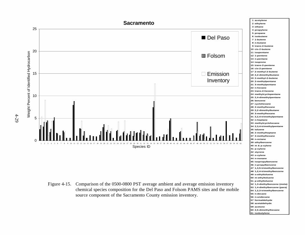
Sacramento

Figure 4-15. Comparison of the 0500-0800 PST average ambient and average emission inventorychemical species composition for the Del Paso and Folsom PAMS sites and the mobilesource component of the Sacramento County emission inventory.

0

5

10

15

20

25

1 2 3 4 5 6 7 8 9 10 11 12 13 14 15 16 17 18 19 20 21 22 23 24 25 26 27 28 29 30 31 32 33 34 35 36 37 38 39 40 41 42 43 44 45 46 47 48 49 50 51 52 53 54 55 56 57 58 59 61 62

Species ID

Wei

ght P

erce

nt o

f Ide

ntifi

ed H

ydro

carb

on

Del Paso

Folsom

EmissionInventory

1 acetylene

2 ethylene

3 ethane

4 propylene

5 propane

6 isobutane

7 1-butene

8 n-butane

9 trans-2-butene

10 cis-2-butene

11 isopentane

12 1-pentene

13 n-pentane

14 isoprene

15 trans-2-pentene

16 cis-2-pentene




20 2-methylpentane

21 3-methylpentane

22 n-hexane

23 trans-2-hexene



26 benzene

27 cyclohexane

28 2-methylhexane


30 3-methylhexane


32 n-heptane



35 toluene

36 2-methylheptane

37 3-methylhexane

38 n-octane

39 ethylbenzene

40 m & p-xylene

41 p-xylene

42 styrene

43 o-xylene

44 n-nonane

45 isopropylbenzene

46 n-propylbenzene



49 o-ethyltoluene

50 m-ethyltoluene

51 p-ethyltoluene




55 n-decane

56 n-undecane

57 formaldehyde

58 acetaldehyde

59 acetone


61 isobutylene

4-29

Sacramento

Figure 4-16. Comparison of the 0500-0800 PST average ambient and average emission inventorychemical species composition for the Del Paso and Folsom PAMS sites and thepoint source component of the Sacramento County emission inventory.

0

5

10

15

20

25

1 2 3 4 5 6 7 8 9 10 11 12 13 14 15 16 17 18 19 20 21 22 23 24 25 26 27 28 29 30 31 32 33 34 35 36 37 38 39 40 41 42 43 44 45 46 47 48 49 50 51 52 53 54 55 56 57 58 59 61 62

Species ID

Wei

ght P

erce

nt o

f Ide

ntifi

ed H

ydro

carb

on

Del Paso

Folsom

EmissionInventory

1 acetylene

2 ethylene

3 ethane

4 propylene

5 propane

6 isobutane

7 1-butene

8 n-butane

9 trans-2-butene

10 cis-2-butene

11 isopentane

12 1-pentene

13 n-pentane

14 isoprene

15 trans-2-pentene

16 cis-2-pentene




20 2-methylpentane

21 3-methylpentane

22 n-hexane

23 trans-2-hexene



26 benzene

27 cyclohexane

28 2-methylhexane


30 3-methylhexane


32 n-heptane



35 toluene

36 2-methylheptane

37 3-methylhexane

38 n-octane

39 ethylbenzene

40 m & p-xylene

41 p-xylene

42 styrene

43 o-xylene

44 n-nonane

45 isopropylbenzene

46 n-propylbenzene



49 o-ethyltoluene

50 m-ethyltoluene

51 p-ethyltoluene




55 n-decane

56 n-undecane

57 formaldehyde

58 acetaldehyde

59 acetone


61 isobutylene

4-30

0

5

10

15

20

25

1 2 3 4 5 6 7 8 9 10 11 12 13 14 15 16 17 18 19 20 21 22 23 24 25 26 27 28 29 30 31 32 33 34 35 36 37 38 39 40 41 42 43 44 45 46 47 48 49 50 51 52 53 54 55 56 57 58

Species ID

Wei

ght P

erce

nt o

f Ide

ntifi

ed H

ydro

carb

on

El Rio

Simi Valley

EmissionInventory

Ventura1 acetylene

2 ethylene

3 ethane

4 propylene

5 propane

6 isobutane

7 1-butene

8 n-butane

9 trans-2-butene

10 cis-2-butene

11 isopentane

12 1-pentene

13 n-pentane

14 isoprene

15 trans-2-pentene

16 cis-2-pentene


18 cyclopentane


20 2-hexene

21 3-methylpentane


23 n-hexane



26 benzene

27 cyclohexane

28 2-methylhexane


30 3-methylhexane


32 n-heptane



35 toluene

36 2-methylheptane

37 3-methylhexane

38 n-octane

39 ethylbenzene

40 m & p-xylene

41 m-xylene

42 p-xylene

43 styrene

44 o-xylene

45 n-nonane

46 isopropylbenzene

47 n-propylbenzene



50 o-ethyltoluene

51 m-ethyltoluene

52 p-ethyltoluene




56 n-decane

57 n-undecane

58 isobutylene

Figure 4-17. Comparison of the 0500-0800 PST average ambient and average emission inventorychemical species composition for the El Rio and Simi Valley PAMS sites and the areasource component of the Ventura County emission inventory.

30%

4-31

Ventura1 acetylene

2 ethylene

3 ethane

4 propylene

5 propane

6 isobutane

7 1-butene

8 n-butane

9 trans-2-butene

10 cis-2-butene

11 isopentane

12 1-pentene

13 n-pentane

14 isoprene

15 trans-2-pentene

16 cis-2-pentene


18 cyclopentane


20 2-hexene

21 3-methylpentane


23 n-hexane



26 benzene

27 cyclohexane

28 2-methylhexane


30 3-methylhexane


32 n-heptane



35 toluene

36 2-methylheptane

37 3-methylhexane

38 n-octane

39 ethylbenzene

40 m & p-xylene

41 m-xylene

42 p-xylene

43 styrene

44 o-xylene

45 n-nonane

46 isopropylbenzene

47 n-propylbenzene



50 o-ethyltoluene

51 m-ethyltoluene

52 p-ethyltoluene




56 n-decane

57 n-undecane

58 isobutylene

Figure 4-18. Comparison of the 0500-0800 PST average ambient and average emissioninventory chemical species composition for the El Rio and Simi Valley PAMSsites and the mobile source component of the Ventura County emission inventory.

0

5

10

15

20

25

1 2 3 4 5 6 7 8 9 10 11 12 13 14 15 16 17 18 19 20 21 22 23 24 25 26 27 28 29 30 31 32 33 34 35 36 37 38 39 40 41 42 43 44 45 46 47 48 49 50 51 52 53 54 55 56 57 58

Species ID

Wei

ght P

erce

nt o

f Ide

ntifi

ed H

ydro

carb

on

El Rio

Simi Valley

EmissionInventory

4-32

Ventura

1 acetylene

2 ethylene

3 ethane

4 propylene

5 propane

6 isobutane

7 1-butene

8 n-butane

9 trans-2-butene

10 cis-2-butene

11 isopentane

12 1-pentene

13 n-pentane

14 isoprene

15 trans-2-pentene

16 cis-2-pentene


18 cyclopentane


20 2-hexene

21 3-methylpentane


23 n-hexane



26 benzene

27 cyclohexane

28 2-methylhexane


30 3-methylhexane


32 n-heptane



35 toluene

36 2-methylheptane

37 3-methylhexane

38 n-octane

39 ethylbenzene

40 m & p-xylene

41 m-xylene

42 p-xylene

43 styrene

44 o-xylene

45 n-nonane

46 isopropylbenzene

47 n-propylbenzene



50 o-ethyltoluene

51 m-ethyltoluene

52 p-ethyltoluene




56 n-decane

57 n-undecane

58 isobutylene

Figure 4-19. Comparison of the 0500-0800 PST average ambient and average emissioninventory chemical species composition for the El Rio and Simi Valley PAMSsites and the point source component of the Ventura County emission inventory.

0

5

10

15

20

25

30

1 2 3 4 5 6 7 8 9 10 11 12 13 14 15 16 17 18 19 20 21 22 23 24 25 26 27 28 29 30 31 32 33 34 35 36 37 38 39 40 41 42 43 44 45 46 47 48 49 50 51 52 53 54 55 56 57 58

Species ID

Wei

ght P

erce

nt o

f Ide

ntifi

ed H

ydro

carb

on

El Rio

Simi Valley

EmissionInventory

4-33

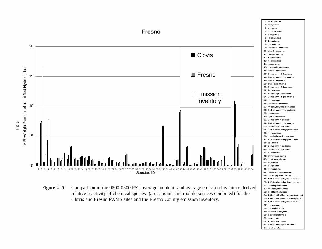
Figure 4-20. Comparison of the 0500-0800 PST average ambient- and average emission inventory-derivedrelative reactivity of chemical species (area, point, and mobile sources combined) for theClovis and Fresno PAMS sites and the Fresno County emission inventory.

Fresno

1 acetylene

2 ethylene

3 ethane

4 propylene

5 propane

6 isobutane

7 1-butene

8 n-butane

9 trans-2-butene

10 cis-2-butene

11 isopentane

12 1-pentene

13 n-pentane

14 isoprene

15 trans-2-pentene

16 cis-2-pentene



19 cis-3-hexene

20 cyclopentane


22 2-hexene

23 3-methylpentane


25 n-hexane

26 trans-2-hexene



29 benzene

30 cyclohexane

31 2-methylhexane


33 3-methylhexane


35 n-heptane



38 toluene

39 2-methylheptane

40 3-methylhexane

41 n-octane

42 ethylbenzene

43 m & p-xylene

44 styrene

45 o-xylene

46 n-nonane

47 isopropylbenzene

48 n-propylbenzene



51 o-ethyltoluene

52 m-ethyltoluene

53 p-ethyltoluene




57 n-decane

58 n-undecane

59 formaldehyde

60 acetaldehyde

61 acetone

62 1,3-butadiene


64 isobutylene

0

5

10

15

20

1 2 3 4 5 6 7 8 9 10 11 12 13 14 15 16 17 18 19 20 21 22 23 24 25 26 27 28 29 30 31 32 33 34 35 36 37 38 39 40 41 42 43 44 45 46 47 48 49 50 51 52 53 54 55 56 57 58 59 60 61 62 63 64

Species ID

MIR

*Wei

ght P

erce

nt o

f Ide

ntifi

ed H

ydro

carb

on

Clovis

Fresno

EmissionInventory

4-34

Sacramento

Figure 4-21. Comparison of the 0500-0800 PST average ambient- and average emission inventory-derived relative reactivity of chemical species (area, point, and mobile sources combined) for the Del Paso and Folsom PAMS sites and the Sacramento County emission inventory.

0

5

10

15

20

1 2 3 4 5 6 7 8 9 10 11 12 13 14 15 16 17 18 19 20 21 22 23 24 25 26 27 28 29 30 31 32 33 34 35 36 37 38 39 40 41 42 43 44 45 46 47 48 49 50 51 52 53 54 55 56 57 58 59 60 61

Species ID

MIR

*Wei

ght P

erce

nt o

f Ide

ntifi

ed H

ydro

carb

on

Del Paso

Folsom

EmissionInventory

1 acetylene

2 ethylene

3 ethane

4 propylene

5 propane

6 isobutane

7 1-butene

8 n-butane

9 trans-2-butene

10 cis-2-butene

11 isopentane

12 1-pentene

13 n-pentane

14 isoprene

15 trans-2-pentene

16 cis-2-pentene




20 2-methylpentane

21 3-methylpentane

22 n-hexane

23 trans-2-hexene



26 benzene

27 cyclohexane

28 2-methylhexane


30 3-methylhexane


32 n-heptane



35 toluene

36 2-methylheptane

37 3-methylhexane

38 n-octane

39 ethylbenzene

40 m & p-xylene

41 p-xylene

42 styrene

43 o-xylene

44 n-nonane

45 isopropylbenzene

46 n-propylbenzene



49 o-ethyltoluene

50 m-ethyltoluene

51 p-ethyltoluene




55 n-decane

56 n-undecane

57 formaldehyde

58 acetaldehyde

59 acetone


61 isobutylene

4-35

Ventura

1 acetylene

2 ethylene

3 ethane

4 propylene

5 propane

6 isobutane

7 1-butene

8 n-butane

9 trans-2-butene

10 cis-2-butene

11 isopentane

12 1-pentene

13 n-pentane

14 isoprene

15 trans-2-pentene

16 cis-2-pentene


18 cyclopentane


20 2-hexene

21 3-methylpentane


23 n-hexane



26 benzene

27 cyclohexane

28 2-methylhexane


30 3-methylhexane


32 n-heptane



35 toluene

36 2-methylheptane

37 3-methylhexane

38 n-octane

39 ethylbenzene

40 m & p-xylene

41 m-xylene

42 p-xylene

43 styrene

44 o-xylene

45 n-nonane

46 isopropylbenzene

47 n-propylbenzene



50 o-ethyltoluene

51 m-ethyltoluene

52 p-ethyltoluene




56 n-decane

57 n-undecane

58 isobutylene

Figure 4-22. Comparison of the 0500-0800 PST average ambient- and average emission inventory-derivedrelative reactivity of chemical species (area, point, and mobile sources combined) for theEl Rio and Simi Valley PAMS sites and the Ventura County emission inventory.

0

5

10

15

20

25

30

35

1 2 3 4 5 6 7 8 9 10 11 12 13 14 15 16 17 18 19 20 21 22 23 24 25 26 27 28 29 30 31 32 33 34 35 36 37 38 39 40 41 42 43 44 45 46 47 48 49 50 51 52 53 54 55 56 57 58

Species ID

MIR

*Wei

ght P

erce

nt o

f Ide

ntifi

ed H

ydro

carb

on

El Rio

Simi Valley

EmissionInventory

4-36

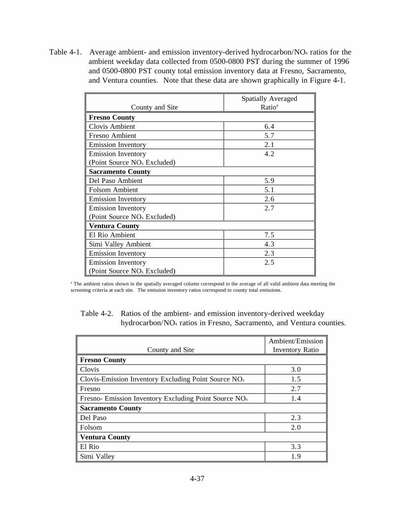
4-37

Table 4-1. Average ambient- and emission inventory-derived hydrocarbon/NOx ratios for theambient weekday data collected from 0500-0800 PST during the summer of 1996and 0500-0800 PST county total emission inventory data at Fresno, Sacramento,and Ventura counties. Note that these data are shown graphically in Figure 4-1.

County and SiteSpatially Averaged

Ratioa

Fresno CountyClovis Ambient 6.4Fresno Ambient 5.7Emission Inventory 2.1Emission Inventory(Point Source NOx Excluded)

4.2

Sacramento CountyDel Paso Ambient 5.9Folsom Ambient 5.1Emission Inventory 2.6Emission Inventory(Point Source NOx Excluded)

2.7

Ventura CountyEl Rio Ambient 7.5Simi Valley Ambient 4.3Emission Inventory 2.3Emission Inventory(Point Source NOx Excluded)

2.5

a The ambient ratios shown in the spatially averaged column correspond to the average of all valid ambient data meeting thescreening criteria at each site. The emission inventory ratios correspond to county total emissions.

Table 4-2. Ratios of the ambient- and emission inventory-derived weekdayhydrocarbon/NOx ratios in Fresno, Sacramento, and Ventura counties.

County and SiteAmbient/EmissionInventory Ratio

Fresno CountyClovis 3.0Clovis-Emission Inventory Excluding Point Source NOx 1.5Fresno 2.7Fresno- Emission Inventory Excluding Point Source NOx 1.4Sacramento CountyDel Paso 2.3Folsom 2.0Ventura CountyEl Rio 3.3Simi Valley 1.9

4-38

Table 4-3. Average ambient- and emission inventory-derived weekday CO/NOx ratios for theambient data collected from 0500-0800 PST during the summer of 1996 and0500-0800 PST county total emission inventory data at Fresno, Sacramento, andVentura counties. Note that these data are shown graphically in Figure 4-2 andno CO data were available for Folsom in 1996.


Ratioa

Fresno CountyClovis Ambient 19.4Fresno Ambient 18.4Emission Inventory 7.1Emission Inventory(Point Source CO and NOx Excluded)

11.4

Sacramento CountyDel Paso Ambient 15.4Emission Inventory 11.4Emission InventoryPoint Source CO and NOx Excluded)

11.9

Ventura CountyEl Rio Ambient 13.1Simi Valley Ambient 22.6Emission Inventory 12.8Emission InventoryPoint Source CO and NOx Excluded)

13.3

a The ambient ratios shown in the spatially averaged column correspond to the average of all valid ambient data meeting thescreening criteria at each site. The emission inventory ratios correspond to county total emissions.

Table 4-4. Ratios of the ambient- and emission inventory-derived weekday CO/NOx

ratios in Fresno, Sacramento, and Ventura counties.

County and SiteAmbient/ Emission

Inventory RatioFresno CountyClovis 2.7Clovis- Emission Inventory Excluding Point Source CO and NOx 1.7Fresno 2.6Fresno- Emission Inventory Excluding Point Source CO and NOx 1.6Sacramento CountyDel Paso 1.4Ventura CountyEl Rio 1.0Simi Valley 1.8

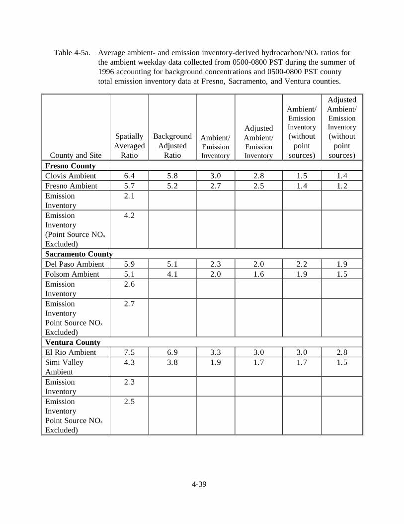
4-39

Table 4-5a. Average ambient- and emission inventory-derived hydrocarbon/NOx ratios forthe ambient weekday data collected from 0500-0800 PST during the summer of1996 accounting for background concentrations and 0500-0800 PST countytotal emission inventory data at Fresno, Sacramento, and Ventura counties.

County and Site

SpatiallyAveraged

Ratio

BackgroundAdjusted

Ratio

Ambient/EmissionInventory

AdjustedAmbient/EmissionInventory

Ambient/EmissionInventory(without

pointsources)

AdjustedAmbient/EmissionInventory(without

pointsources)

Fresno CountyClovis Ambient 6.4 5.8 3.0 2.8 1.5 1.4Fresno Ambient 5.7 5.2 2.7 2.5 1.4 1.2EmissionInventory

2.1

EmissionInventory(Point Source NOx

Excluded)

4.2

Sacramento CountyDel Paso Ambient 5.9 5.1 2.3 2.0 2.2 1.9Folsom Ambient 5.1 4.1 2.0 1.6 1.9 1.5EmissionInventory

2.6

EmissionInventoryPoint Source NOx

Excluded)

2.7

Ventura CountyEl Rio Ambient 7.5 6.9 3.3 3.0 3.0 2.8Simi ValleyAmbient

4.3 3.8 1.9 1.7 1.7 1.5

EmissionInventory

2.3

EmissionInventoryPoint Source NOx

Excluded)

2.5

4-40

Table 4-5b. Average ambient- and emission inventory-derived CO/NOx ratios for theambient weekday data collected from 0500-0800 PST during the summer of1996 accounting for background concentrations and 0500-0800 PST countytotal emission inventory data at Fresno, Sacramento, and Ventura counties.

County and Site

SpatiallyAveraged

Ratio

BackgroundAdjusted

Ratio

Ambient/EmissionInventory

AdjustedAmbient/EmissionInventory

Ambient/EmissionInventory(without

pointsources)

AdjustedAmbient/EmissionInventory(without

pointsources)

Fresno CountyClovis Ambient 19.4 14.6 2.7 2.1 1.7 1.4Fresno Ambient 18.4 14.8 2.6 2.5 1.6 1.2EmissionInventory

7.1

EmissionInventory(Point SourceNOx and COExcluded)

11.4

Sacramento CountyDel PasoAmbient

15.4 8.1 1.4 0.7 1.3 0.7

EmissionInventory

11.4

EmissionInventoryPoint SourceNOx and COExcluded)

11.9

Ventura CountyEl Rio Ambient 13.1 8.2 1.0 0.7 1.0 0.6Simi ValleyAmbient

22.6 19.2 1.8 1.5 1.7 1.4

EmissionInventory

12.8

EmissionInventoryPoint SourceNOx and COExcluded)

13.3

4-41

Table 4-6. Summary of the Saturday ambient average TNMOC, NOx, and CO data meetingall validity and screening criteria at Fresno, Clovis, and Del Paso Manor.

Site ID Site Name, County# ValidSamples

AverageTNMOC

ppbCbAverageNOx ppbc

Average COppb

060190008 Fresno 1st Street,Fresno

4 275 44 900

060195001 Clovis, Fresno 4 315 30 742060670006 Del Paso Manor,

Sacramento4 228 29 507

a Only valid samples collected on Saturdays from July through September 1996 (begin hours 0500, 0600, and 0700 PST) meeting allscreening criteria were used to calculate the averages in the table.b TNMOC = Total Non-Methane Organic Compounds includes both identified and unidentified compounds. Averages were calculated forall valid samples with TNMOC > 100 ppbC.c NOx averages were calculated for all valid samples with NOx > 10 ppb to eliminate NOx values at or near instrument detection limits.

Table 4-7. Average ambient- and emission inventory-derived Saturday hydrocarbon/NOx

ratios for the ambient data collected from 0500-0800 PST during the summerof 1996 and 0500-0800 PST county total emission inventory data for Fresnoand Sacramento counties. Note that these data are shown graphically inFigures 4-3 and 4-4.

County and Site Spatially Averaged Ratioa

Fresno County

Clovis Ambient 10.7

Fresno Ambient 6.4

Saturday Emission Inventory 2.2Saturday Emission Inventory(Point Source NOx Excluded) 4.8

Sacramento County

Del Paso Ambient 10.0


a The ambient ratios shown in the spatially averaged column correspond to the average of all valid ambient data collected onSaturdays meeting the screening criteria at each site. The emission inventory ratios correspond to county total emissions.

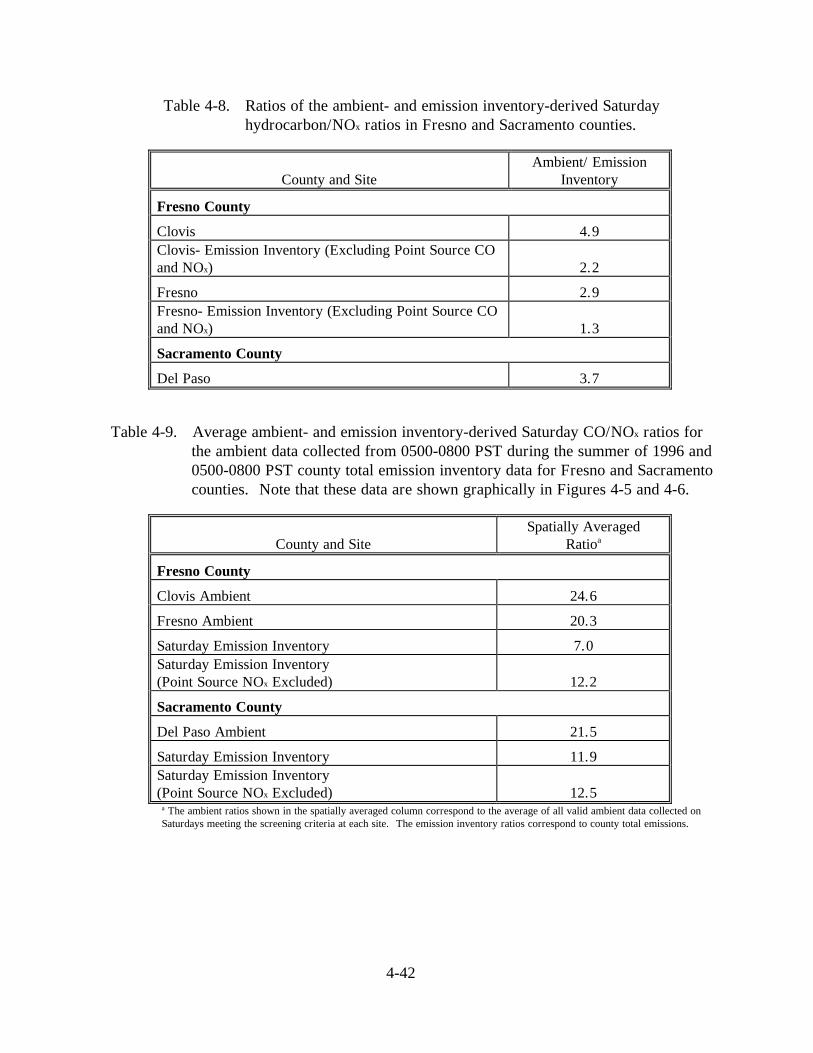
4-42

Table 4-8. Ratios of the ambient- and emission inventory-derived Saturdayhydrocarbon/NOx ratios in Fresno and Sacramento counties.

County and SiteAmbient/ Emission

Inventory

Fresno County

Clovis 4.9Clovis- Emission Inventory (Excluding Point Source COand NOx) 2.2

Fresno 2.9Fresno- Emission Inventory (Excluding Point Source COand NOx) 1.3

Sacramento County

Del Paso 3.7

Table 4-9. Average ambient- and emission inventory-derived Saturday CO/NOx ratios forthe ambient data collected from 0500-0800 PST during the summer of 1996 and0500-0800 PST county total emission inventory data for Fresno and Sacramentocounties. Note that these data are shown graphically in Figures 4-5 and 4-6.


Ratioa

Fresno County

Clovis Ambient 24.6

Fresno Ambient 20.3


Sacramento County

Del Paso Ambient 21.5


a The ambient ratios shown in the spatially averaged column correspond to the average of all valid ambient data collected onSaturdays meeting the screening criteria at each site. The emission inventory ratios correspond to county total emissions.

4-43

Table 4-10. Ratios of the ambient- and emission inventory-derived SaturdayCO/NOx ratios in Fresno and Sacramento counties.

County and SiteAmbient/ EmissionInventory Ratios

Fresno County

Clovis 3.5Clovis- Emission Inventory (Excluding Point Source COand NOx) 2.0

Fresno 2.9Fresno- Emission Inventory (Excluding Point Source COand NOx) 1.7

Sacramento County

Del Paso 1.8

[BLANK PAGE]

5-1

5. CONCLUSIONS FROM THE EMISSION INVENTORYEVALUATION AND RECOMMENDATIONS

Comparisons between ambient data and emission estimates for hydrocarbon, CO, andNOx are based on the premise that early morning ambient pollutant concentrations (whenemissions are high, and wind speed, atmospheric mixing height, and chemical reactivity arelow) are dominated by fresh emissions in the vicinity of the monitor. In this study,comparisons of the ambient- and emission inventory-derived hydrocarbon/NOx and CO/NOx

ratios as well as comparisons of individual hydrocarbon species compositions were made forsix PAMS monitoring sites located in Fresno, Sacramento, and Ventura counties (two sites ineach county). The ambient data used in this comparison were collected from 0500-0800 PSTduring the summer of 1996.

To further maximize the influence of nearby emissions and minimize the influence oftransported emissions, periods with generally high average ambient hydrocarbonconcentrations were selected for analysis at each site. In order to obtain a useful number ofsamples with sufficiently high concentrations above instrument detection limits, minimumhydrocarbon and NOx thresholds of 100 ppbC and 10 ppb, respectively, were established.

The daily speciated emission inventory was prepared by the ARB. Daily totalemissions were speciated and temporally allocated to the 0500-0800 time period using profilecode cross-reference files and source category code files provided by the ARB. The inventorywas then converted from a mass to a molar basis and placed on a common basis with theambient data to include only the chemical species capable of being detected by the PAMSmonitoring systems.

The strength of a top-down emission inventory evaluation is that it can be used toidentify areas of an emission inventory that appear to be suspect. This methodology cannot beused to quantify the absolute errors in an inventory, but can be used to compare the relativeamounts of pollutants in the inventory and the ambient air. The chemical species analysis canbe used to characterize the chemical composition of the inventory and the ambient air and helpto identify which major source types of the inventory appear to need improvement.

5.1 CONCLUSIONS – HYDROCARBON/NOX AND CO/NOX RATIO ANALYSES

Significant differences between the 1996 ambient data and the 1996 ARB inventory forFresno, Sacramento, and Ventura counties exist at the sites examined in this study. Thefollowing conclusions summarize the major findings of the hydrocarbon/NOx and CO/NOx

ratio analyses:

• In general, weekday ambient hydrocarbon/NOx ratios at the two sites in Fresno andSacramento are fairly consistent within each county, while ambient ratios at the two sites inVentura County are quite different. This indicates that ambient concentrations in Fresnoand Sacramento counties are fairly uniform throughout the counties, while in Ventura

5-2

County, there are concentration gradients in the ambient air throughout the county.Consequently, the county-wide average emission inventory ratios do not compare well witheither ambient site in Ventura County and the inventory is not spatially resolved enough tomake robust recommendations based on the ratio comparisons. Conversely, we believethat the relatively even concentrations between site pairs in Sacramento and Fresno countiesallow the reasonable use of county-wide emissions in the ratio comparisons.

• Ratio comparisons were made for cases both including and excluding point sourceemissions. In Sacramento and Ventura counties, point source NOx emissions are notsignificant during the 0500-0800 PST time period and therefore do not affect the emissionsratios. However, in Fresno County, point sources contribute about 35 percent of total NOx

emissions during the morning time period. Consequently, excluding point source NOx

emissions from the ratio calculations significantly changed the ambient-ratio to emissioninventory-ratio comparisons.

• In Fresno County, the weekday ambient hydrocarbon/NOx ratio is approximately a factorof 3 higher than the inventory when all emissions sources are included in the ratiocalculation and about a factor of 1.5 to 2.0 when point source NOx is excluded from thecalculation. Area and mobile sources are the main contributors to hydrocarbon emissions inFresno County. Because these are the dominant emissions sources, it is likely that thehydrocarbon component of these categories is underestimated and/or the NOx component isoverestimated.

• In general, the results of the weekday hydrocarbon/NOx ratio comparisons indicate that thehydrocarbon component of the emission inventory appears to be underestimated by a factorof 2.0 to 2.5 in Sacramento County and 2.0 to 4.0 in Ventura County. Area and mobilesources are the main contributors to emissions in Sacramento and Ventura counties.Because these are the dominant emissions sources, it is likely that the hydrocarboncomponent of these categories is underestimated, and/or the NOx component isoverestimated.

• The results of the weekday CO/NOx ratio comparisons indicate that the ambient CO/NOx

ratios are approximately a factor of 2 higher than emissions ratios in Fresno and Venturacounties, and a factor of 1.5 higher in Sacramento County. This suggests that the COcomponent of the inventory is underestimated and/or the NOx component is overestimated.

• The results of the Saturday hydrocarbon/NOx and CO/NOx ratio comparisons indicate that,on average, Saturday ambient hydrocarbon concentrations are higher than weekdayconcentrations while NOx concentrations are lower. Consequently, the Saturday ambientratios are significantly higher than the weekday ambient ratios. The hydrocarbon/NOx andCO/NOx ratios in the emission inventory do not vary significantly between the weekdayand Saturday inventories. It appears as though the Saturday emission inventory is notrepresentative of Saturday ambient conditions.

• While the mass of hydrocarbon, NOx, and CO are slightly different between the weekdayand Saturday emission inventories, it appears that no adjustment was made for weekendtemporal profile assignments.

5-3

• In general, adjusting ambient concentrations to account for the influence of backgroundconcentrations led to a small improvement in the comparisons between ambient- andemission inventory-derived ratios.

5.2 CONCLUSIONS – HYDROCARBON SPECIES ANALYSES

The following conclusions summarize the major findings of the individual hydrocarbonspecies and species group analyses:

• This comparison shows that while the emission composition and the ambientcompositions in Fresno and Sacramento counties are in generally good agreement, thereis a consistent underestimation of the less reactive compounds and an overestimation ofthe more reactive compounds.

• In Ventura County, ambient data from Simi Valley follows a similar pattern to that inFresno and Sacramento counties (e.g., slight underestimation of paraffins andoverestimation of olefins and aromatics). However, at the El Rio site in VenturaCounty, the concentration of ambient paraffins is much higher than in the inventory,and the concentration of ambient olefins and aromatics is much lower than in theemission inventory. The contributions of paraffins to the total hydrocarbons at El Rioare also much higher than at any of the other sites and likewise the contributions ofolefins and aromatics are much lower than at any of the other sites. We can speculatethat the increased paraffins may be associated with natural geogenic oil and gas seepsoffshore of Ventura County which may not be fully accounted for in the emissionsindustry.

• In general, the individual species composition comparisons indicate that there areseveral compounds in the emission inventory that are either (1) not individuallyidentified or (2) reported below detection limits. One of these compounds isisopentane, an abundant compound in the ambient air that is quite reactive. Isopentaneshould be identified in the emission inventory.

• In Ventura County, species compositions between the two ambient sites aresignificantly different indicating that the chemical composition of the ambient air inVentura County varies throughout the county. The county-wide average inventory doesnot correspond well with either ambient site, which show large differences as wellbetween the two sites’ ambient species compositions.

• There are uncertainties associated with the spatial matching of ambient data and thecounty-wide emission inventory data. Such uncertainties are apparent for all threecounties in the case of ethane. The major sources of ethane in Fresno and Sacramentocounties are from livestock. We speculate that ethane in Ventura County may beassociated with natural geogenic oil and gas seeps offshore of Ventura County. Whilethe absolute mass of ethane emissions from these categories may be correct in theinventory, it appears that ethane from these sources is not detected in the vicinity of theambient monitors. Consequently, in the species comparison plots, there are largediscrepancies in the ambient- and emission inventory-derived ethane compositions.

5-4

• Significant differences between ambient and area source emission inventory acetyleneethane, ethylene, propane, propylene, and formaldehyde compositions in Fresno andSacramento counties may be indicative of the emission inventory containing too mucharea source combustion activity from 0500-0800 PST. Ethane is also characteristic ofevaporative emissions from vehicle refueling which may be misrepresented during thistime period. Vehicle refueling evaporative profiles may not reflect properties of thenewly reformulated fuels in use in California.

• In Fresno County, differences between area source emissions compositions of benzene,xylenes, and acetone suggest that the area source speciation profiles for Fresno Countymay not accurately represent benzene and xylene solvent use in the area. The mobilesource emissions compositions indicate that the mobile source exhaust speciationprofiles may not accurately reflect benzene compositions in fuel.

• In Fresno and Sacramento counties, differences between ambient and emissionscompositions of propane and formaldehyde indicate that the mobile source exhaustspeciation profiles do not accurately represent these compounds.

• In Sacramento County, differences between ambient and emissions compositions ofisobutane, n-butane, n-hexane, and cyclohexane suggest that evaporative emissionsfrom vehicle refueling or the transporting of petroleum products is misrepresented inthe inventory.

• In Ventura County, chemical species compositions of ethane, propane, and n-butane atEl Rio suggest that this site is influenced by a natural gas combustion source, and/orpetroleum production sources while species compositions at Simi Valley suggest thatthis site is primarily influenced by area and mobile source emissions.

• Although the Ventura County inventory does not compare well with either site, thepoint source component of the inventory appears to better match ambient chemicalcompositions at the El Rio site.

• Discrepancies in emissions and ambient chemical compositions of the followingcompounds are important when assessing the reactivity of the inventory and the ambientair: isopentane, toluene, trimethylbenzenes, diethylbenzenes, 1-butene.

5.3 RECOMMENDATIONS

The following recommendations on possible improvements to the emission inventoryare based on the results and conclusions of the emission inventory reconciliation.

• Area and mobile sources combined constitute approximately 80 percent of the totalhydrocarbon component of the emission inventory while point sources contribute theremaining 20 percent. Because area and mobile sources are the dominant categories inthe inventory, future inventory improvement should focus on these source categories.

• Temporal profile assignments in the Saturday emission inventory should be reviewedand revised as necessary to reflect weekend emissions activity.

5-5

• The apparent under-estimation of absolute mass of hydrocarbon, NOx, and COemissions from area and mobile source categories should be investigated.

• The top area and mobile source emissions sub-categories should be identified andreviewed. The speciation profiles used to disaggregate the hydrocarbon emissionsshould be reviewed as well as the temporal code assignments.

• The following source categories are likely assigned unrepresentative speciation and/ortemporal profiles: area source fuel combustion, gasoline refueling evaporativeemissions, gasoline exhaust emissions, and petroleum product storage andtransportation.

• A bottom-up evaluation of the inventory should be performed including review ofemissions sources and activity data in each region.

• It is recommended that the emission inventory be gridded for future top-downevaluations.

[BLANK PAGE]

6-1

6. REFERENCES

Air Resources Board (1997) Public meeting to consider approval and verification of theCalifornia emission inventory. Report prepared by the Technical Support Division,Mobile Source Control Division, Office of Air Quality and Transportation Planning,California Environmental Protection Agency, Air Resources Board, Sacramento, CA,November.

Carter W.P.L. (1994) Development of ozone reactivity scales for volatile organic compounds.J. Air & Waste Manag. Assoc. 44, 881-899.

Fujita E.M., Croes B.E., Bennett C.L., Lawson D.R., Lurmann F.W., and Main H.H. (1992)Comparison of emission inventory and ambient concentration ratios of CO, NMOG,and NOx in California's South Coast Air Basin. J. Air & Waste Manag. Assoc. 42,264-276.

Fujita E.M., Watson J.G., Chow J.C., and Lu Z. (1994) Validation of the chemical massbalance receptor model applied to hydrocarbon source apportionment in the SouthernCalifornia Air Study. Environ. Sci. Technol. 28, 1633-1649.

Gertler A.W. and Pierson W.R. (1996) Recent measurements of mobile source emissionfactors in North American Tunnels. Science Total Environment 189-190, 107-113.

Haste T.L., Chinkin L.R. Main H.H., Kumar N., and Roberts P.T. (1998a) Analysis of Datafrom the 1995 NARSTO-Northeast Study Volume II: Use of PAMS Data to Evaluate aRegional Emission Inventory. Final report prepared for Coordinating ResearchCouncil, Atlanta, GA by Sonoma Technology, Inc., Petaluma, CA under subcontract toENVIRON International Corp., Novato, CA, STI-95424-1737-FR, March.

Haste T.L., Chinkin L.R., Kumar N., Lurmann F.W., and Hurwitt S.B. (1998b) Use ofAmbient Data Collected During IMS-95 to Evaluate a Regional Emission Inventory forthe San Joaquin Valley. Final report prepared for San Joaquin Valleywide AirPollution Study Agency c/o California Air Resources Board, Sacramento, CA bySonoma Technology, Inc., Petaluma, CA, STI-997211-1800-FR, July.

Korc M.E., Roberts P.T., Chinkin L.R., and Main H.H. (1993) Comparison of emissioninventory and ambient concentration ratios of CO, NMOC, and NOx in the LakeMichigan Air Quality Region. Draft final report prepared for Lake Michigan AirDirectors Consortium, Des Plaines, IL by Sonoma Technology, Inc., Santa Rosa, CA,STI-90218-1357-DFR, October.

Korc M.E., Roberts P.T., Chinkin L.R., Lurmann F.W., and Main H.H. (1995)Reconciliation of emission inventory and ambient data for three major regional airquality studies. In Transactions - Regional Photochemical Measurement and ModelingStudies, pp. 176-194

[BLANK PAGE]

A-1

APPENDIX A

HYDROCARBON SPECIES MEASURED AT CLOVIS, FRESNO,DEL PASO, FOLSOM, EL RIO, AND SIMI VALLEY

DURING THE SUMMER OF 1996

[BLANK PAGE]

Table A-1. Hydrocarbon species measured at the Clovis, Fresno 1st Street, Del Paso, Folsom, El Rio, and Simi Valley PAMSmonitoring sites during the summer of 1996.

Clovis Fresno Del Paso Folsom El Rio Simi Valley

acetylene acetylene acetylene acetylene acetylene acetylene

ethylene ethylene ethylene ethylene ethylene ethylene

ethane ethane ethane ethane ethane ethane

propylene propylene propylene propylene propylene propylene

propane propane propane propane propane propane

isobutane isobutane isobutane isobutane isobutane isobutane

1-butene 1-butene 1-butene n-butane 1-butene 1-butene

n-butane n-butane n-butane isopentane n-butane n-butane

trans-2-butene trans-2-butene trans-2-butene 1-pentene trans-2-butene trans-2-butene

cis-2-butene cis-2-butene cis-2-butene n-pentane cis-2-butene cis-2-butene

trimethylbenzene trimethylbenzene isopentane isoprene isopentane isopentane

isopentane isopentane 1-pentene trans-2-pentene 1-pentene 1-pentene

1-pentene 1-pentene n-pentane 2-methyl-2-butene n-pentane n-pentane

n-pentane n-pentane isoprene 2,2-dimethylbutane isoprene isoprene

isoprene isoprene trans-2-pentene cis-3-hexene trans-2-pentene trans-2-pentene

trans-2-pentene trans-2-pentene cis-2-pentene cyclopentane cis-2-pentene cis-2-pentene

cis-2-pentene cis-2-pentene 2-methyl-2-butene 2-methyl-2-butene 2,2-dimethylbutane 2,2-dimethylbutane

2-methyl-2-butene 2-methyl-2-butene 2,2-dimethylbutane 2-hexene cyclopentane cyclopentane

2,2-dimethylbutane 2,2-dimethylbutane cis-3-hexene 3-methylpentane 2-methyl-2-butene 2-methyl-2-butene

cis-3-hexene cis-3-hexene 2-methyl-2-butene n-hexane 2-hexene 2-hexene

cyclopentane 4-methylpentene 2-hexene cis-2-hexene 3-methylpentane 3-methylpentane

2-methyl-2-butene cyclopentane 3-methylpentane methylcyclopentane 2-methyl-1-pentene 2-methyl-1-pentene

2-hexene 2-methyl-2-butene n-hexane 2,4-dimethylpentane n-hexane n-hexane

3-methylpentane 2-hexene trans-2-hexene benzene methylcyclopentane methylcyclopentane


2-methyl-1-pentene 3-methylpentane cis-2-hexene cyclohexane 2,4-dimethylpentane 2,4-dimethylpentane

n-hexane 2-methyl-1-pentene methylcyclopentane 2-methylhexane benzene benzene

trans-2-hexene n-hexane 2,4-dimethylpentane 2,2-dimethylbutane cyclohexane cyclohexane

cis-2-hexene trans-2-hexene benzene 3-methylhexane 2-methylhexane 2-methylhexane

methylcyclopentane cis-2-hexene cyclohexane 2,2,4-trimethylpentane 2,2-dimethylbutane 2,2-dimethylbutane

2,4-dimethylpentane methylcyclopentane 2-methylhexane n-heptane 3-methylhexane 3-methylhexane

benzene 2,4-dimethylpentane 2,2-dimethylbutane methylcyclohexane 2,2,4-trimethylpentane 2,2,4-trimethylpentane

cyclohexane benzene 3-methylhexane 2,3,4-trimethylpentane n-heptane n-heptane

2-methylhexane cyclohexane 2,2,4-trimethylpentane toluene methylcyclohexane methylcyclohexane

2,2-dimethylbutane 2-methylhexane n-heptane 2-methylheptane 2,3,4-trimethylpentane 2,3,4-trimethylpentane

3-methylhexane 2,2-dimethylbutane methylcyclohexane 3-methylhexane toluene toluene

2,2,4-trimethylpentane 3-methylhexane 2,3,4-trimethylpentane n-octane 2-methylheptane 2-methylheptane

n-heptane 2,2,4-trimethylpentane toluene ethylbenzene 3-methylhexane 3-methylhexane

methylcyclohexane n-heptane 2-methylheptane m & p-xylene n-octane n-octane

2,3,4-trimethylpentane methylcyclohexane 3-methylhexane o-xylene ethylbenzene ethylbenzene

toluene 2,3,4-trimethylpentane n-octane n-nonane m & p-xylene m & p-xylene

2-methylheptane toluene ethylbenzene isopropylbenzene m-xylene m-xylene

3-methylhexane 2-methylheptane m & p-xylene n-propylbenzene p-xylene p-xylene

n-octane 3-methylhexane p-xylene 1,3,5-trimethylbenzene styrene styrene

ethylbenzene n-octane styrene 1,2,4-trimethylbenzene o-xylene o-xylene

m & p-xylene ethylbenzene o-xylene o-ethyltoluene n-nonane n-nonane

styrene m & p-xylene n-nonane m-ethyltoluene isopropylbenzene isopropylbenzene

o-xylene p-xylene isopropylbenzene p-ethyltoluene n-propylbenzene n-propylbenzene

n-nonane styrene n-propylbenzene 1,3-diethylbenzene (meta) 1,3,5-trimethylbenzene 1,3,5-trimethylbenzene

isopropylbenzene o-xylene a-pinene 1,4-diethylbenzene (para) 1,2,4-trimethylbenzene 1,2,4-trimethylbenzene

n-propylbenzene n-nonane 1,2,4-trimethylbenzene n-decane o-ethyltoluene o-ethyltoluene

a-pinene isopropylbenzene b-pinene n-undecane m-ethyltoluene m-ethyltoluene

1,3,5-trimethylbenzene n-propylbenzene o-ethyltoluene 2,5-dimethylhexane p-ethyltoluene p-ethyltoluene


1,2,4-trimethylbenzene a-pinene m-ethyltoluene isobutylene 1,3-diethylbenzene (meta) 1,3-diethylbenzene (meta)

b-pinene 1,3,5-trimethylbenzene p-ethyltoluene 1,4-diethylbenzene (para) 1,4-diethylbenzene (para)

o-ethyltoluene 1,2,4-trimethylbenzene 1,3-diethylbenzene (meta) 1,2,3-trimethylbenzene 1,2,3-trimethylbenzene

m-ethyltoluene b-pinene 1,4-diethylbenzene (para) n-decane n-decane

p-ethyltoluene o-ethyltoluene 1,2,3-trimethylbenzene n-undecane n-undecane

1,3-diethylbenzene (meta) m-ethyltoluene n-decane isobutylene isobutylene

1,4-diethylbenzene (para) p-ethyltoluene n-undecane

1,2,3-trimethylbenzene 1,3-diethylbenzene (meta) formaldehyde

n-decane 1,4-diethylbenzene (para) acetaldehyde

n-undecane 1,2,3-trimethylbenzene acetone

formaldehyde n-decane 1,3-butadiene

acetaldehyde n-undecane 1-hexene

acetone formaldehyde 2,5-dimethylhexane

1,3-butadiene acetaldehyde isobutylene

2,5-dimethylhexane acetone

isobutylene 1,3-butadiene

2-methyl-1-butene

1-hexene

2,2,4-trimethylpentane

2,5-dimethylhexane

2,4-dimethylhexane

2,3-dimethylhexane

2,2-dimethylpropane

isobutylene

Documents

THE USE OF PAMS DATA TO EVALUATE REGIONAL EMISSION · PDF fileTami L. Haste-Funk Lyle R. Chinkin ... The u se of PAMS data to evaluate regional emission inventories in California