Embed Size (px)
Citation preview
THE VA~~ONAL METHOD FOR TKE CALCULATION OF RO-VISIONAL ENERGY LULLS
and
1986
NORTH-HOLLAND - Amsterdam
116 S. Carter, N. C. Handy / Variational method for m-vibrational energy levels
Contents
1. h-mx.luction. .............................................. 118 2. The position of the variational method for vibrational energy levels in 1976 . . 122 3. The derivation of the kineiic energy operator for polyatomic systems ....... 123 4. Kinetic energy operators T for various coordinate systems .............. 134 5. The potential energy function, V. ................................ 146 6. A vibration-rotation variational procedure using p(R,, R,, 8) ........... 154 7. Conclusion. ............................................... 168
References .................................................. 169
Computer Physics Reports 5 (1986) 115-172 Norm-Holland. Amsterdam
117
THE VARIATIONAL METHOD FOR THE CALCULATION OF RO-VIBRATIONAL ENERGY LEVELS
S. CARTER
department of Chemists, Universi~ of Read@ ~ite~ights, Reading RG6 2AL), UK
and
N.C. HANDY
University Chemical Laboratory, Lensfield Road, Cambridge CB2 I E W, UK
Received 21 August 1986
In this paper the current status of the variational method for the determination of the rotational-vibrational energy levels of polyatomic systems is reviewed. Special attention is made for the derivation of the kinetic energy operator in various coordinate systems, and several forms are given. Similarly, analytic forms which are in current use for the potentials are given. The calculation of the Hamiltonian matrix elements (expansion functions, numerical integration grid points and weights) is described in detail, and a description of our programs for this problem is given in section 6.
0167-7977/W/$20.30 0 Elsevier Science Publishers B.V. (North-Holland Physics Publishing Division)
118 S. Carter, N. C. Handy / Variational method for ro-vibrational energy levels
1. Introduction
The last decade has seen the r~o~ition that the variational method has a contribution to make in the calculation of vibration-rotation energy levels of a polyatomic molecules. The problem to be solved may be stated very simply: given a potential energy surface in an analytical form, what are the vibration-rotation energy levels? Of course, it is desirable to obtain the associated wavefunctions at the’same time, and if property surfaces are available, it should then be possible to calculate transition matrix elements.
The relevance of spectroscopy is immediate. Spectroscopists are measuring an increasing number of levels for small and medium sized molecules. Our purpose ultimately must be the better understanding of the nature of potential energy surfaces. One of the best tests that we known for analytic potential energy surfaces is that they should reproduce all these experimental levels. Furthe~ore, if an~ytical representations of the dipole (or higher moment) surfaces are available, then tests of these representations come from comparison with experimental transition moments.
Potential energy functions derived from only limited spectroscopic data (geometry, harmonic force constants) and thermochemical data (bond strengths) have a vital role to play, when linked to the variational method, in assisting the spectroscopist in his experimental studies (see in particular the techniques discussed in sections 5.6 and 6). For example, by reproducing only a very few well established vibrational band origins, the combination of a ‘good’ potential function and a ‘good’ basis set can be used in variational calculations to predict very accurate vibrational levels that are not included in the derivation of the potential. It follows that the spectroscopist can use the va~ational method to predict ~brational band origins, which will be of use during his assignment of the spectra. Furthermore, having established a potential form which correctly predicts the vibrational spectra for one isotope, the variational method can be used to predict the positions of spectral lines for other isotopes.
There is a further aspect of the variational method that can be used to great advantage by the spectroscopist. The variational method, as a matter of course, provides eigenfunctions of the various vibrational levels. Providing that ‘good’ basis functions in a ‘good’ coordinate system are used, these eigenfunctions can then be used to assign the spectra in the domain for which the coordinates are most valid. These eigenfunctions can also be used to evaluate matrix elements involving ab initio expansions of the dipole moment to predict line intensities, which is of further use to the spectroscopist.
The variational method is straightfo~~~y applied. Given a Ha~lto~~ fi and some expansion functions arp,, the secular equations
(1.1‘1 s=l
are solved for the eigenvalues q and the eigenvectors Ci. If we denote the eigenvalues for it4 expansion functions in ascending order by WlM, W$“, . . . , TV,,, then MacDonald’s theorem [l] states that
S. Carter, N.C. Handy / Variational method for ro-vibrational energy levels 119
This theorem shows the advantages and weaknesses of the variational method. The great advantage is that all the eigenvalues are upper bounds to the corresponding exact eigenvalues; the great weakness is that the addition of extra expansion functions will always lower the eigenvalues, and one is never sure to what accuracy the eigenvalues are obtained at any given stage, the only test apparently being that the addition of extra expansion functions should not lower the required eigenvalues significantly. At this stage it must be recalled that one may typically be interested in the lowest 50 eigenvalues (if J = 0), if J Z 0 then (2 J + 1) times as many. To achieve convergence for such a number of eigenvalues, M, the number of expansion functions, has to be large (for 50 eigenvalues, M may have to be 500), and so we reach the difficulty that large matrices have to be worked with, and up to 20% of their eigenvalues obtained. Throughout this review it will be assumed that the matrix can be held in the main memory of the computer, and diagonalised there. For most workers this means that the dimension of the largest matrices lie in the range 200 to 700 (or perhaps 2000 with the very latest computers).
It is one of the problems of the next few years to increase this dimension to 5000 or so (there are many problems in physical chemistry for which this is desirable, for example coupled channel problems in reactive scattering [2]). It is well known that ab initio theoretical chemists can deal routinely with matrices whose dimension exceeds 100000 but they have two advantages namely (a) that their matrices are sparse (90% or more) and (b) that they usually want only the lowest one or two eigenvalues. It is therefore unlikely that their methods can be directly applied to the problem of vibrational level determination.
Returning to the secular equations (l.l), the choice of expansion functions is crucially important if the dimension of the matrix is to be minimal. Before this can be answered it is necessary to decide on the coordinate system for the problem. For the lowest vibrations, it has long been recognised that normal coordinates Q are appropriate, but for higher vibrational states these become inappropriate and should be replaced by some internal coordinates X One of the recent discoveries has been the importance of local modes [3] in excited vibrational states, and these are best represented by bond coordinates, and certainty not by normal coordinates. The other main argument in favour of internal coordinates is that the potential energy V must be invariant to rotations, it will be so if expressed in terms of 5I, but not if represented in terms of a truncated normal coordinate expansion.
In a laboratory fixed axis system, an N atom molecule’s position is described by 3N coordinates X. The motion of the centre of mass G is not relevant to the problem, and so it has to be removed from the problem. It is also usual to introduce three Euler angles (Y, p and y to describe the orientation of some ‘molecule-fixed axes’ relative to the laboratory fixed axes. The remaining 3N - 6 coordinates will be either normal coordinates or internal coordinates. There are of course an infinity of ways to define the molecule fixed axes. The problem is again easily stated: given an arbitrary position of the molecule with respect to the laboratory fixed axes, how may a Cartesian axes system be tied to the molecule? It is important to do this because the relative orientation of these two axis systems is described by Euler angles, and for any position of the molecule, it must be possible to attribute unique values for (Y, p and y.
Having decided on the definition of the body fixed axis system, and also on the choice of normal coordinates or a particular set of internal coordinates it is then necessary to derive the form of the kinetic energy operator f in terms of these coordinates. In fact it is usual to express
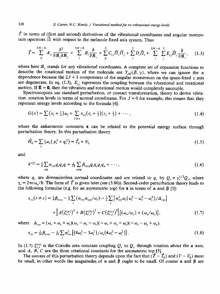
:[g] d pm x) 30 suxw XI! x 103 (do1 ~~11aumlCs~ uv .x03 ~8~a)aym1.1o3 %uf~\o~~o3 aql
01 spaallCIoay1 uogaqmlJad .I~~.IO-puoaas '((9g.g) aas).tala~ ua~@ so s 3ou1303 aye *~/%xxL~ ="x
aJaqM “(&/;A='a dq "b 01 palF?Ial a&? pm! SalXXUp.IOO:, It?WnOU SSaIUO~SUaUUp a.%%? "b aJaqM
W) ‘
. . .
s<r
0-f ‘
*** ~(~+s~~~~+~ff)s~x~ +~~~~+~~~~=~~)~ :[~]epm~o3 aye 01 "au~p-tocm SI~A~I A&ma luasaldaJ
Icay leyl suaaw SKI 'aIdumxa ~03 0 =r 30~ XWX.T~~J~~~, IIKUJOU 30 stu.xal UT SI~AC+I uogalo;r-uog
-tzqF ahgap 01 hzoaql 'uoym1o3su~~11 ~tmluo:, 10 ‘uoy-eqmlmd psepuvls asn slsydo~soncmds
~a~dnomtd~a~a~duro:,p~noMuo~lom~m.rogrtlo.rpu~ uorlmqyayl uaql 'o= 331 TO~OUI
@uoyt?103 pug @ucywq1\ aql uaaMlaq ftugdno3 a$1 sluasalda~"~~ ‘(E'T) -ba III *almma%ap am
SF z pay3-amds ayl uo umluaurom .n@ua aql30 sluauodutoo 1 +fz ayl asnmaq amapuadap
x) aql a.tou%; um aM a.myM ‘(A 'd)"'x a3E apmaf0u.t atg 30 uofloru p2uofl~lo3 ayt aq!map
01 suo~l~.rn3 uotsmdxa 30 3as awldmo3 v -saw~~p.~oor, pmoymq~ dut! 303 spmls !K a.wy aJay;ll
S. Carter, N.C. Handy / Variational method for ro-vibrational energy levels 121
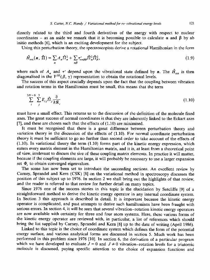
directly related to the third and fourth derivatives of the energy with respect to nuclear coordinates - as an aside we remark that it is becoming possible .to calculate IX and /3 by ab initio methods [6], which is an exciting development for the subject.
Using this perturbation theory, the spectroscopists derive a rotational Hamiltonian in the form
where each of A, and r’ depend upon the vibrational state defined by n. The fir,,, is then diagonalised in the YJ”(/3, y) representation to obtain the rotational levels.
The success of this aspect crucially depends upon the fact that the coupling between vibration and rotation terms in the Hamiltonian must be small, this means that the term
3N-6 3
(1.10)
must have a small effect. This returns us to the discussion of the definition of the molecule fixed axes. The great success of normal coordinates is that they are inherently linked to the Eckart axes [7], and these are chosen such that the effects of (1.10) are minimised.
It must be recognised that there is a great difference between perturbation theory and variation theory in the discussion of the effects of (1.10). For normal coordinate perturbation theory it must be sufficient to go no further than second order to take account of the effects of (1.10). In variational theory the term (1.10) forms part of the kinetic energy expression, which enters every matrix element in the Hamiltonian matrix, and it is, at least from a theoretical point of view, irrelevant to discuss the size of these coupling matrix elements. In practice it will matter, because if the coupling elements are large, it will probably be necessary to use a larger expansion set @r to obtain converged eigenvalues.
The scene has now been set to introduce the succeeding sections. An excellent review by Carney, Sprandel and Kern (CSK) [8] on the variational method in spectroscopy discusses the position of this subject up to 1976. In section 2 we shall bring out the highlights of that review, and the reader is referred to that review for further detail on many topics.
Since 1976 one of the success stories in this topic is the elucidation by Sutcliffe [9] of a straightforward method to derive the kinetic energy operator in any internal coordinate system. In Section 3 this approach is described in detail. It is important because the kinetic energy operator is complicated, and past attempts to derive such hamiltonians have been fraught with serious errors. In section 4, it will be seen that several vibration-rotation kinetic energy operators are now available with certainty for three and four atom systems. Here, these various forms of the kinetic energy operator are reviewed with, in particular, a list of references which should bring the list supplied by Camey, Sprandel and Kern [8] up to the date of writing (April 1986).
Linked to this topic is the choice of coordinate system which defines the form of the potential energy surface, and various analytical forms are discussed in section 5. Much work has been performed in this problem since 1976 [lo]. In section 6, the derivation of a particular program which we have developed to evaluate J = 0 and J # 0 vibration-rotation levels for a triatomic molecule is discussed, paying specific attention to the choice of expansion functions and
122 S. Carter, N. C. Handy / Variational method for ro-vibrational energy levels
integration techniques employed. It will be shown how the program, which uses a hamiltonian expressed in terms of bond lengths and bond angle, can be linked to a potential energy surface optimisation procedure.
2. The position of the variational method for vibrational energy levels in 1976
By this time it was recognised that the perturbation theory approach had severe shortcomings especially if the molecule contains large amplitude (bending) vibrational motions. Therefore workers were looking at the variational approach and ref. [8] discusses in detail the successful applications of the method to diatomic molecules. In this context it was recognized that the expansion of the potential I/ as
was not so compact as the alternative Simons-Parr-Finlan [ll] form
V= xc:,(AR/R)“, (2.2) n
mainly because the latter series is convergent in [1/2R,, co] instead of [0, 2R,] for the Dunham expansion [12]. Much of the work on diatomics carries over to larger systems, for example the use by Suzuki [13] of a harmonic oscillator expansion set, with analytic evaluation of the matrix elements. On the other hand Zetik and Matsen [14] used the HEG (Harrison, Engerholm and Gwinn [15]) numerical quadrature scheme, to take advantage of pointwise determined potential energy curves. CSK also refer to the fact that Greenawalt and Dickinson [16] found Morse-oscil- lator basis sets more rapidly convergent than harmonic oscillator basis sets for diatomic molecules.
In their sections on polyatomic molecules, CSK introduced several coordinate systems and associated kinetic energy operators. The important simplification of the Darling and Dennison Hamiltonian by Watson [17] yields the simple Hamiltonian given by (3.85) in this review, for normal coordinates. CSK also give a Hamiltonian appropriate for an isosceles geometry due to Carney et al. They also give for the first time the correct form for the kinetic energy operator in terms of two bond lengths (R,, Rlj and the enclosed bond angle 8, ascribing it to Lai and Hagstrom [18] and Sprandel and Kern [8].
For the normal coordinate system, Whitehead and Handy [19] used an expansion set involving the product of harmonic oscillator functions - they evaluated the matrix elements numerically using Gauss-Hem&e quadrature schemes. On the other hand Lai and Hagstrom, and Sprandel and Kern solved Self-Consistent Field-like equations to obtain good one-variable expansion functions, and Sprandel and Kern did a CI-type calculation on top of this. CSK demonstrate that by 1976 workers were also using Morse Oscillator expansion functions with analytic integration methods. In summary the position was that applications to triatomic molecules were in full swing, with correct Hamiltonians being used for normal coordinates or internal coordi- nates; and mostly numerical methods being used for matrix element evaluation. Matrices of the size of 220 were being diagonalised for H,O for example.
S. Carter, N.C. Handy / Variational method for ro-vibrational energy levels 123
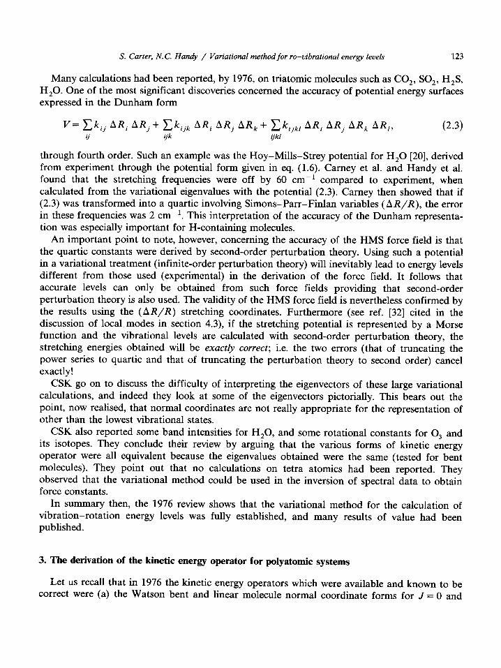
Many calculations had been reported, by 1976, on triatomic molecules such as CO,, SO,, H,S, H,O. One of the most significant discoveries concerned the accuracy of potential energy surfaces expressed in the Dunham form
V= xkij AR, ARj -I- zkijk ARi AR, AR, + xkijk, ARi ARj AR, AR,, ij ijk ijkl
(2.3)
through fourth order. Such an example was the Hoy-Mills-Strey potential for H,O [20], derived from experiment through the potential form given in eq. (1.6). Camey et al. and Handy et al. found that the stretching frequencies were off by 60 cm-’ compared to experiment, when calculated from the variational eigenvalues with the potential (2.3). Camey then showed that if (2.3) was transformed into a quartic involving Simons-Parr-Finlan variables (AR/R), the error in these frequencies was 2 cm- ‘. This interpretation of the accuracy of the Dunham representa- tion was especially important for H-containing molecules.
An important point to note, however, concerning the accuracy of the HMS force field is that the quartic constants were derived by second-order perturbation theory. Using such a potential in a variational treatment (infinite-order perturbation theory) will inevitably lead to energy levels different from those used (experimental) in the derivation of the force field. It follows that accurate levels can only be obtained from such force fields providing that second-order perturbation theory is also used. The validity of the HMS force field is nevertheless confirmed by the results using the (AR/R) stretching coordinates. Furthermore (see ref. [32] cited in the discussion of local modes in section 4.3), if the stretching potential is represented by a Morse function and the vibrational levels are calculated with second-order perturbation theory, the stretching energies obtained will be exactly correct; i.e. the two errors (that of truncating the power series to quartic and that of truncating the perturbation theory to second order) cancel exactly!
CSK go on to discuss the difficulty of interpreting the eigenvectors of these large variational calculations, and indeed they look at some of the eigenvectors pictorially. This bears out the point, now realised, that normal coordinates are not really appropriate for the representation of other than the lowest vibrational states.
CSK also reported some band intensities for H,O, and some rotational constants for 0, and its isotopes. They conclude their review by arguing that the various forms of kinetic energy operator were all equivalent because the eigenvalues obtained were the same (tested for bent molecules). They point out that no calculations on tetra atomics had been reported. They observed that the variational method could be used in the inversion of spectral data to obtain force constants.
In summary then, the 1976 review shows that the variational method for the calculation of vibration-rotation energy levels was fully established, and many results of value had been published.
3. The derivation of the kinetic energy operator for polyatomic systems
Let us recall that in 1976 the kinetic energy operators which were available and known to be correct were (a) the Watson bent and linear molecule normal coordinate forms for J = 0 and
124 S. Carter, N.C. Handy / Variational method for ro-vibrational energy levels
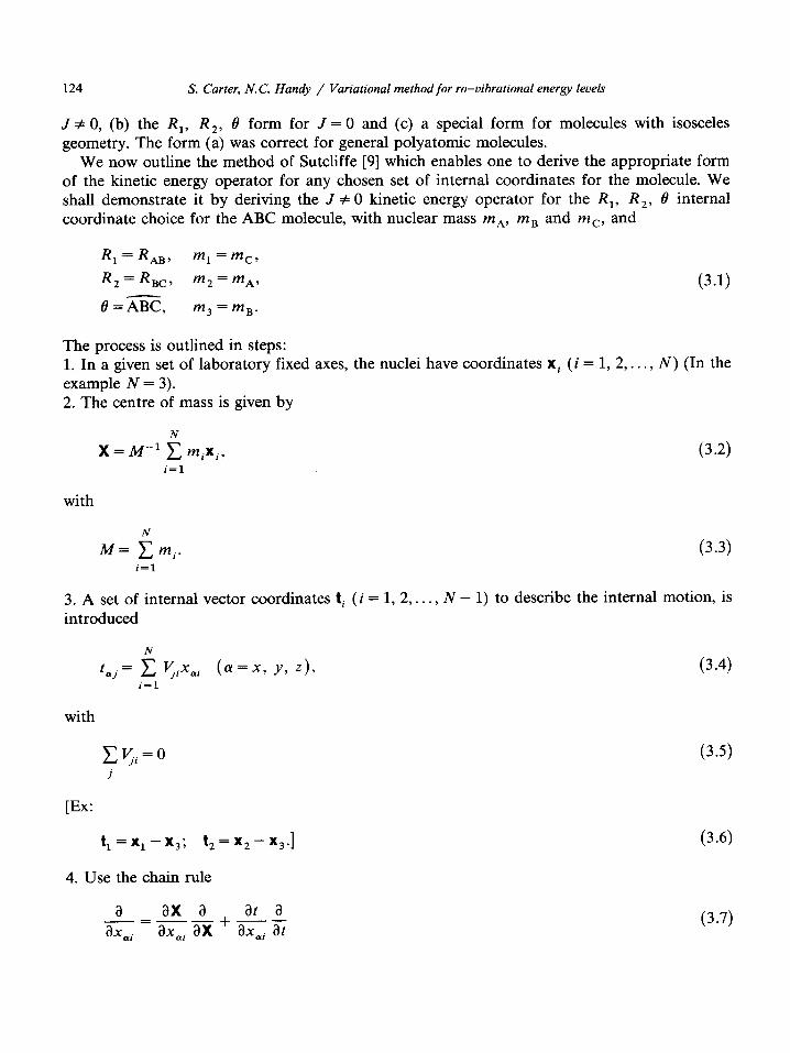
J # 0, (b) the R,, R,, 8 form for J = 0 and (c) a special form for molecules with isosceles geometry. The form (a) was correct for general polyatomic molecules.
We now outline the method of Sutcliffe [9] which enables one to derive the appropriate form of the kinetic energy operator for any chosen set of internal coordinates for the molecule. We shall demonstrate it by deriving the J # 0 kinetic energy operator for the R,, R,, 8 internal coordinate choice for the ABC molecule, with nuclear mass mA, mB and m,, and
R, = %a, m,=m,,
Rz= RBc, m2= mAP (3.1)
0=X5?, m3 = mB.
The process is outlined in steps: 1. In a given set of laboratory fixed axes, the nuclei have coordinates xi (i = 1, 2,. . . , N) (In the example N = 3). 2. The centre of mass is given by
N
)( = Me’ 2 mixi, i=l
with
M= $mi. i=l
3. A set of internal introduced
vector coordinates ti (i = 1, 2,
taj= t QXai (a =x, y, z), i=l
with
Cb$=O
[Ex:
t, =x, -x,; t, = x2 - x,.]
. . . , N - 1) to describe the internal motion, is
(3.2)
(3.3)
(3.4)
(3.5)
(3-b)
4. Use the chain rule
_2EL+ a at a -- axe, axdi ax ax,, at (3.7)
S. Carter, N.C. Handy / Variational method for ro-vibrational energy levels
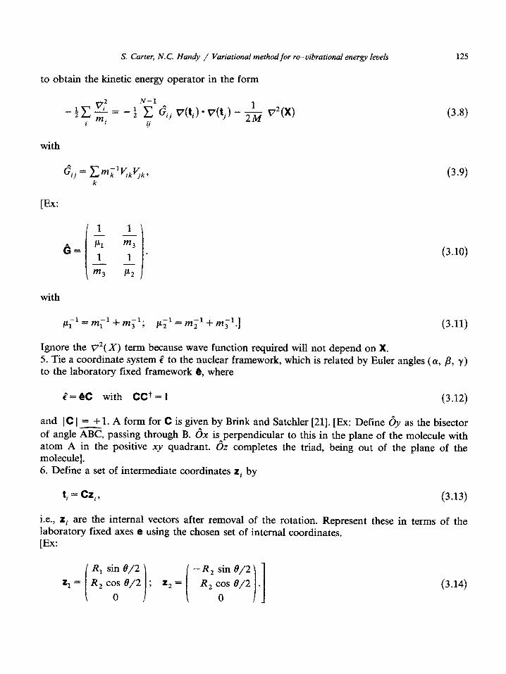
to obtain the kinetic energy operator in the form
-ix 2 = - 3 y ejj v&j l v(tj) - & v*(x)
i l ij
with
Gij = Crn,l~,~,,
[Ex:
with
k
1 1
K m3 1 1 -
m3 E
-1 Pl = m,’ + m;l
125
(3 4
W)
(3.10)
-1 P2 = m;’ + m;l.] (3.11)
Ignore the v2( X) term because wave function required will not depend on X. 5. Tie a coordinate system P to the nuclear framework, which is related by Euler angles (cy, /3, y) to the laboratory fixed framework @, where
t-.&C with CCt=I (3.12)
and (C]= + 1. A form for C is given by Brink and Satchler [21]. [Ex: Define b;, as the bisector of angle z, passing through B. 8~ is perpendicular to this in the plane of the molecule with atom A in the positive xy quadrant. 6.z completes the triad, being out of the plane of the molecule]. 6. Define a set of intermediate coordinates zi by
ti = Cr,,
i.e., zi are the internal vectors after removal of the rotation. Represent laboratory fixed axes e using the chosen set of internal coordinates. [Ex:
z, = R, sini?/
R, cos 8/2
0
-R, sin 8/2
; z,= R, cos 8/2
0 il
(3.13)
these in terms of the
(3.14)
126 S. Carter, N.C. Handy / Variational method fir ro-vibrational energy Ievels
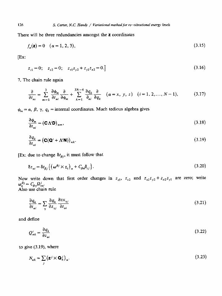
There will be three redundancies amongst the z coordinates
f,(z)=0 (a=l,2,3),
[Ex:
2 21 =e 0; z,2 = 0; Z,pzy~ + Zyl.z,~ = 0.1
7. The chain rule again
a -= 3&?$a atfxi
c -+ c m=l %li a% ~~~~6~~ (a=~, y, z) (i=l,2 ,.._, N-l),
a,
c+~ = EY, p, y, qk = internal coordinates. Much tedious algebra gives
> = (C&D),,, ar
2 = (C(Qi + tiN>),,. #xl
[Ex: due to change Stsj, it must follow that
IjZ,i = Gfsj (( ,‘j X Zi) Q C Ca*Sij ).
(3.15)
(3.16)
(3.17)
(3.18)
(3.19)
(3.20)
Now write down that first order changes in zzl, zz2 and zx1zy2 -t z,~z~~ are zero; write ikPj = C&a;,. Ako use chain rule
aa a% azxd -=~-- atai Y
aZ, atai
and define
to give (3.19), where
~~~ = c(zjx a{),. j
(3.21)
(3.22)
(3.23)
S. Carter, N.C. Handy / Variational method for ro-vibrational energy levels 127
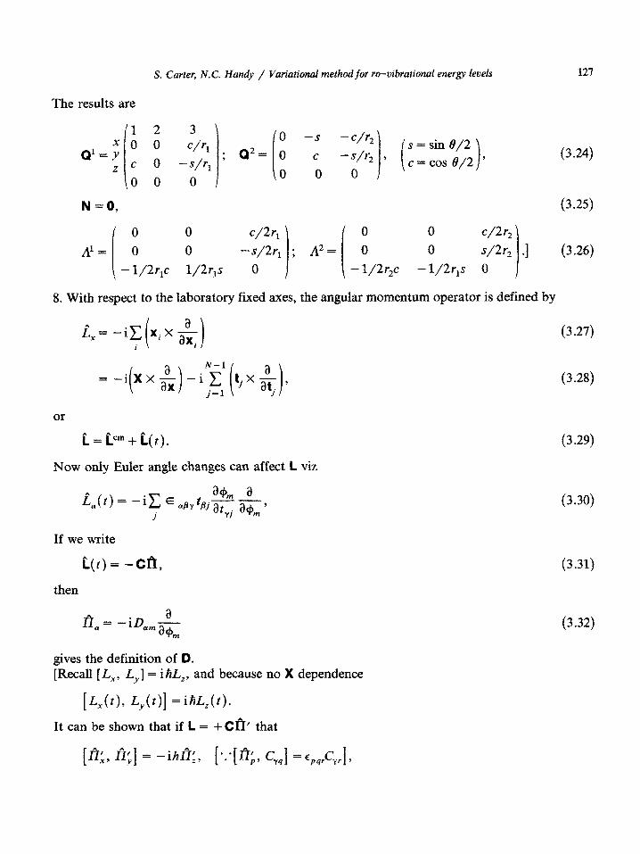
The results are
‘12 3 x0 0
Q1 = Y ze 0
_;;r’; Q’=[; -% ~~~~, (;+;;j), (3.24)
\oo 01
N =O, (3.25)
i
0 0 c/25 0
Al= 0 0 -S/25 ; AZ= 0 (3.26)
-I/2r,c 1/2r,s 0
! i
- 1/2r,c
8. With respect to the laboratory fixed axes, the angular momentum operator is defined by
= -i(X~$)-i~~(tjX$-)!
(3.27)
, (3.28)
or
L=P+i(t).
Now only Euler angle changes can affect L viz
(3.29)
If we write
i(t) = -cfI,
then
gives the definition of D. [Recall [L,, L,,] = i hL,, and because no X dependence
[ &(O, $W] = iW0.
It can be shown that if L = +CI?Ii, that
(3.30)
(3.31)
(3.32)
128 S. Carter, N.C. Handy / Variational method for ro-vibrational energy levels
now
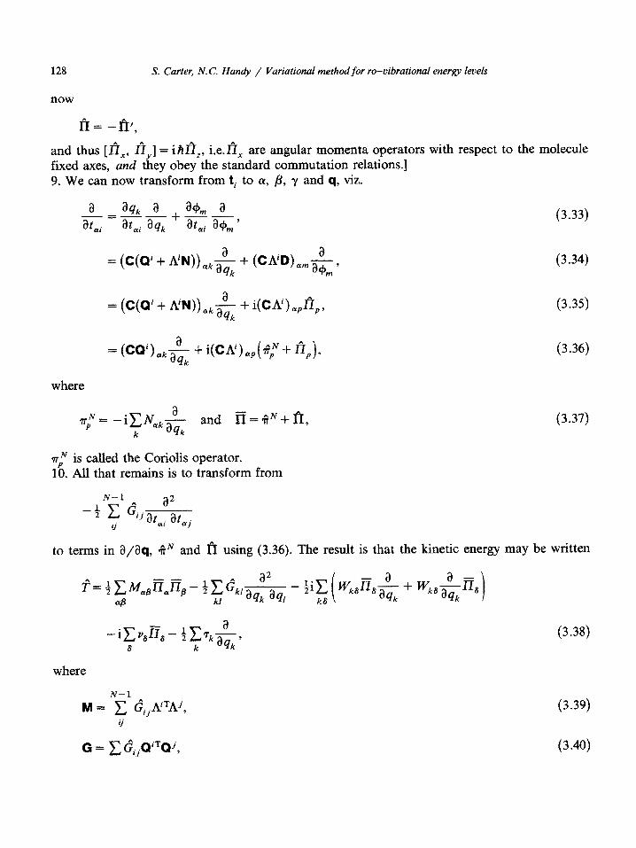
and thus [I?,, I?,,] = i M?,, i.e. fi, are angular momenta operators with respect to the molecule fixed axes, and they obey the standard commutation relations.] 9. We can now transform from ti to cy, p, y and q, viz.
where
a aqk a --- at,i- %%l a
%i %k + atai a+, 7
= (C(@ + ITN)),,; + (C&D).&, qk m
= (C(Q' + tiN)) ak-$- + i(C&) &?IP, k
= (cQi)ak& -t i(ck),p( ti; + fiP),
N a I$ = -izNakaq, and iI=ii”+fi,
k
(3.33)
(3.34)
(3.35)
(3.36)
(3.37)
rN is called the Coriolis operator. 15. All that remains is to transform from
N-l
-4 t: ‘ijat Tit ij al nj
to terms in a/aq, 4iN and f!I using (3.36). The result is that the kinetic energy may be written
where
G = z eijQiTQj,
(3.38)
(3.39)
(3.40)
S. Curter, N.C. Handy / Variationaf method for ro-vibrational energy levels
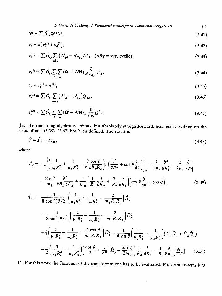
w = C eijQiThj,
129
(3.41)
7-j2)= cGjjc z(Q’+ LYN)~,+&. (3.47) I a I
[Ex: the remaining algebra is tedious, but absolutely straightforward, because everything on the r.h.s. of eqs. (3.39)-(3.47) has been defined. The result is
?= fv + &a, (3.48)
where
_L+l_ a
~1% ~2%
-+cot&gj ----
ii
1 ;t2 1 a2 --
+ %I aR,z 2P2 aR;
cos 9 a2 +
1 la la --
-- -- mB aR, aR, K RI 3R2 -I- R, aR,
(3.49)
(3.50)
11. For this work the Jacobian of the tr~sform~tions has to be evaluated. For most systems it is
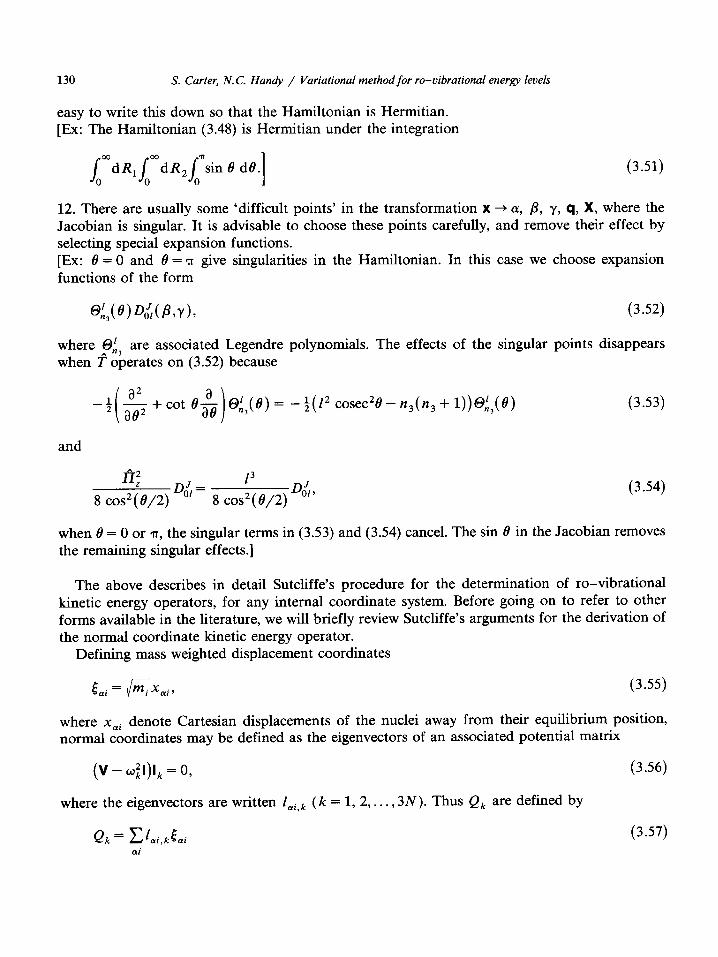
130 S. Carter, N.C. Handy / Variational method for ro-vibrationaI energy Ievels
easy to write this down so that the Hamiltonian is Hermitian. [Ex: The Hamiltonian (3.48) is Hermitian under the integration
(3.51)
12. There are usually some ‘difficult points’ in the transformation x --) (11, j3, y, q, X, where the Jacobian is singular. It is advisable to choose these points carefully, and remove their effect by selecting special expansion functions. [Ex: 8 = 0 and 8 = 7~ give singularities in the Hamiltonian. In this case we choose expansion functions of the form
where pi, are associated Legendre when T operates on (3.52) because
polynomials. The effects of the singular points disappears
and
7=P 13 --2
8 cos2 (e/2) D,:= -
8 c02( 812) %
- $( l2 c0sec2e - P& + l))@(e) (3.53)
(3.54)
when 8 = 0 or IT, the singular terms in (3.53) and (3.54) cancel. The sin 8 in the Jacobian removes the remaining singular effects.]
The above describes in detail Sutcliffe’s procedure for the determination of ro-vibrational kinetic energy operators, for any internal coordinate system. Before going on to refer to other forms available in the literature, we will briefly review Sutcliffe’s arguments for the derivation of the normal coordinate kinetic energy operator.
Defining mass weighted displacement coordinates
(3.55)
where xai denote Cartesian displacements of the nuclei away from their equilibrium position, normal coordinates may be defined as the eigenvectors of an associated potential matrix
(v - w;I)I, = 0, (3.56)
where the eigenvectors are written luiak (k = 1, 2,. . . ,3N). Thus Qk are defined by
Q/c = C lai,ktai ai
(3.57)
131
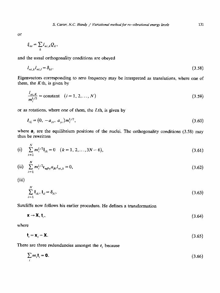
or
and the usual orthogonality conditions are obeyed
Egenvectors corresponding to zero frequency may be interpreted as translations, where one of them, the Kth, is given by
& mv2
=constant (i=l,Z,...,N) I
(3.59)
or as rotations, where one of them, the Lth, is given by
li, = (O, I‘“*i, nyj)mi’2$ (3.60)
where aj are the equilibrium positions of the nuclei. The orthogonality conditions (3.58) may thus be rewritten
(i) ~~f’~l~~=O (k=1,2 ,..., 3N-61, (3.61)
(ii) (3.62) i=l
(iii)
Sutdiffe now follows his earlier procedure. He defines a tr~sformation
x-+x,ti,
where
ti = xi I x.
There are three redundancies amongst the ti because
xWtjtj = 0.
(3.63)
(3.64)
(3.65)
(3.66)
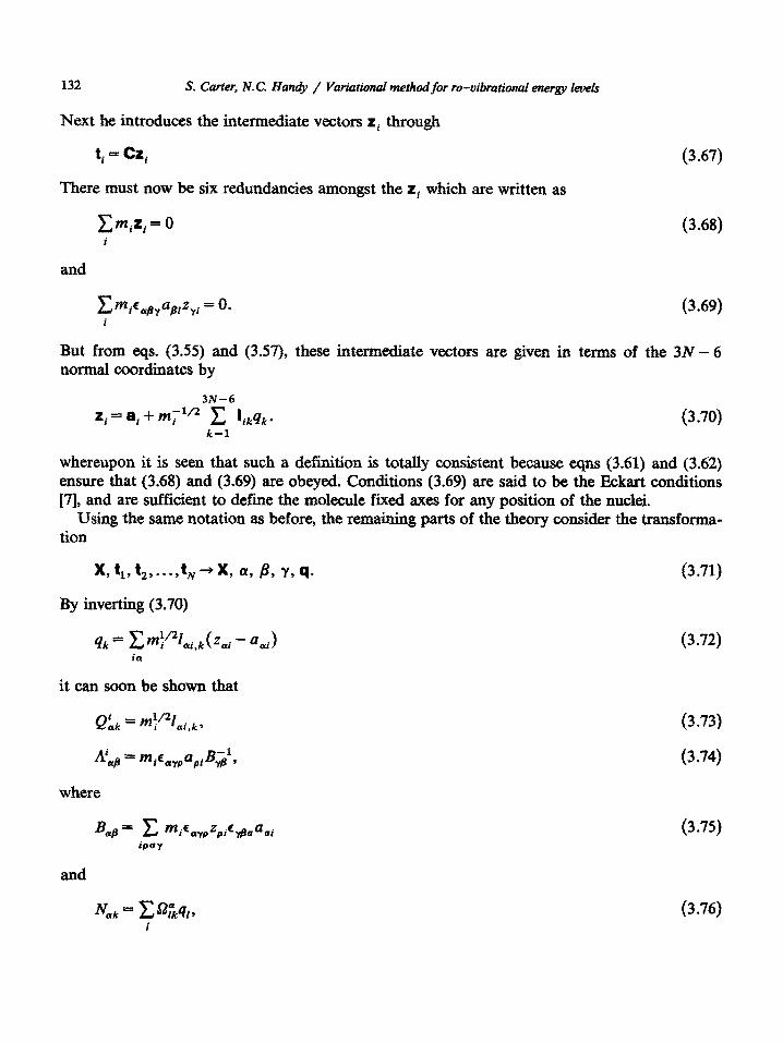
132 S. Carter, N.C. Handy / Variational method for ro-vibrational energy levels
Next he introduces the intermediate vectors zi through
ti = Cr,
There must now be six redundancies amongst the zi which are written as
(3.67)
c m,z, = 0 (3.68)
and
ItI miiQa8yugizyi = 0. (3.69) i
But from eqs. (3.55) and (3.57), these ~te~~ate vectors are given in terms of the 3N - 6 normal coordinates by
3N-6
‘i = e,+m;‘fl c likqk. (3.70) k-l
whereupon it is seen that such a definition is totally consistent because eqns (3.61) and (3.62) ensure that (3.68) and (3.69) are obeyed. Conditions (3.69) are said to be the Eckart conditions [7], and are sufficient to define the molecule fixed axes for any position of the nuclei.
Vsing the same notation as before, the remaining parts of the theory consider the transforma- tion
x, t,, t,,...,t, + K a, la, Y, q* (3.71)
By inverting (3.70)
qk t ~m:‘2zai,k(zai - ‘ai) ia
it can soon be shown that
where
B a/3 = C mi~aypzpibYgaaai
WY
and
(3.72)
(3.73)
(3.74)
(3.75)
(3.76)
S. Carter, N.C. Handy / Variational method for ro-vibrational energy levels
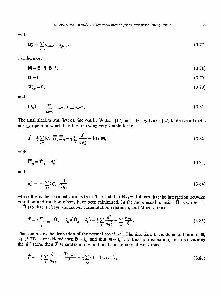
with
133
(3.77)
Furthermore
M = B-‘I,B-‘, (3.78)
G= I, (3.79)
Jq,, = 0, (3.80)
and
(3.81)
The final algebra was first carried out by Watson [17] and later by Louck [22] to derive a kinetic energy operator which had the following very simple form:
with
n,=fi,+;I,” (3.83)
and
(3.82)
where this is the so called coriolis term. The fact that W,, = 0 shows that the interaction between vibration and rotation effects have been minimised. In the more usual notation I? is written as -I? (so that it obeys anomalous commutation relations), and M as 1-1, thus
(3.85)
This completes the derivation of the normal coordinate Hamiltonian. If the dominant term in B, eq. (3.75), is considered then B - I,, and thus M - I; ‘. In this approximation, and also ignoring the ,fiN term, then f separates into vibrational and rotational parts thus
a2 $-ix-- k ad
(3.86)
134 S. Carter, N.C. Handy / Variational method for ro-vibrational energy IeveIs
which is the usual “zeroth order” form for the vibration-rotation kinetic energy operator, and forms the basis of perturbation theory.
In principle the Sutcliffe formalism can be used to derive the form of the vibration-rotation kinetic energy operator for any coordinate system, for any polyatomic molecule. However from the above it will be apparent that the whole process is extraordinarily messy algebraically; the only successful way to proceed will be through an algebraical language. Other forms for the kinetic energy operator which have been derived for three and four atom systems are given in the next chapter.
4. Kinetic energy operators ? for various coordinate systems
The past decade has seen considerable advances in the derivation of kinetic energy operators, and their subsequent use in variational calculations of the ro-vibrational energy levels of small polyatomic molecules. In this section we highlight the principal forms of operators and coordinate systems which are used in this context. Examples of kinetic energy operators which are used in the full variational context are those expressed in internal coordinates (section 4.5), in closed-coupled coordinates (section 4.6), in normal coordinates (section 4.4), and in hyperspheri- cal coordinates (section 4.2). For larger systems and for higher ro-vibrational levels it is not possible to use the full variational theory, and approximations must be introduced. For example, this has been very successfully done in the framework of the non-rigid bender Hamiltonian (section 4.1) and in the study of local-vs.-normal vibrations (section 4.3). We apologise that this chapter can only be a brief and very incomplete examination of all the various methods that are used for the determination of ro-vibrational levels of polyatomic molecules. In particular we are aware that we have given scant attention to those methods which decouple vibrational and rotational motions. However such theories lie behind the whole of modem-day spectroscopy.
4.1. Non-rigid bender and related Hamiltonians
Although these methods of calculation are not entirely variational, they deserve special mention since they represent the transition from the more conventional perturbation treatment to the now popular variational procedure. It is the inadequate treatment, by the perturbation technique, of certain vibrations that has led to the popularity of the variational procedure in recent years, and the non-rigid bender and related methods were the first to tackle such vibrations variationally.
As long ago as 1970, Hougen, Bunker and Johns [23] had derived the complete quantum mechanical kinetic energy operator for triatomic molecules in a coordinate system which was designed for use in rigid bender calculations. In more recent years, Bunker, Jensen and co-workers have developed this Hamiltonian further for application to semi-rigid and non-rigid benders [24,25]. An excellent review article by Jensen has appeared in this Journal [26], which outlines the non-rigid bender technique fully, and so only the highlights of the method will be given here.
The essence of the approach is to separate the ‘floppy’ bending vibration (which limits the perturbation technique) from the ‘fast’ stretching vibrations (cf. the Born-Oppenheimer sep-
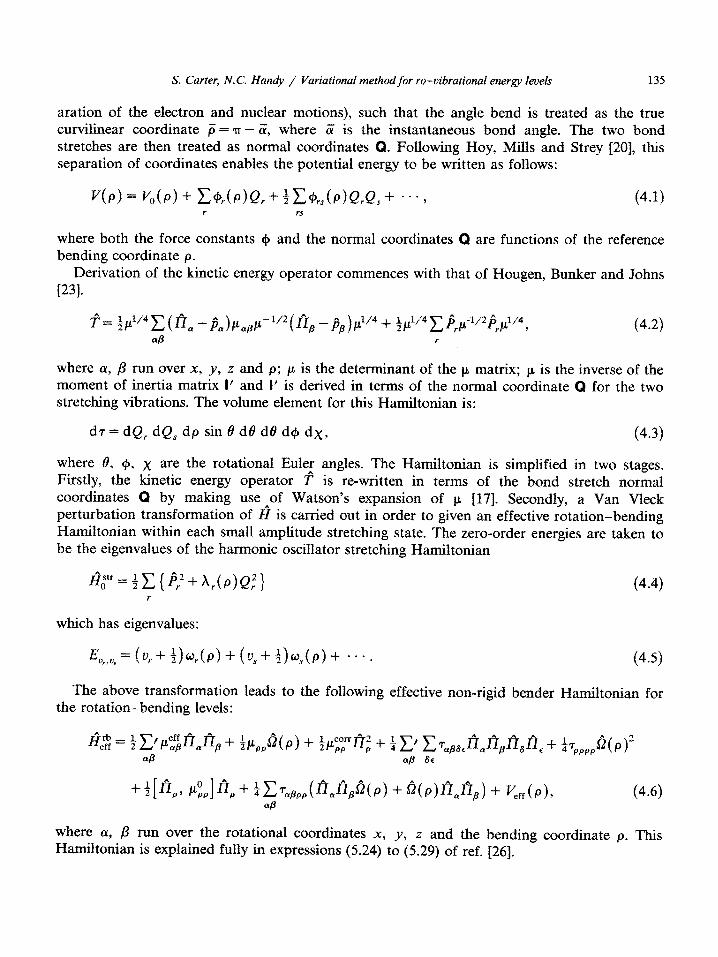
S. Carter, N.C. Handy / Variational method for ro-vibrational energy ieveis 135
aration of the electron and nuclear motions), such that the angle bend is treated as the true cu~ilinear coordinate ii = T - ci; where Z is the instantaneous bond angle. The two bond stretches are then treated as normal coordinates Q. Following Hoy, Mills and Strey [20], this separation of coordinates enables the potential energy to be written as follows:
(4.1)
where both the force constants Cp and the normal coordinates Q are functions of the reference bending coordinate p.
Derivation of the kinetic energy operator commences with that of Hougen, Bunker and Johns
]231.
where cy, @ run over X, y, z and p; p is the determinant of the u matrix; p is the inverse of the moment of inertia matrix I’ and I’ is derived in terms of the normal coordinate Q for the two stretching vibrations. The volume element for this Hamiltonian is:
dr = dQ, dQ, dp sin 9 dtI d0 d4p dx, (4.3)
where 6, (p, x are the rotational Euler angles. The Hamiltonian is simplified in two stages. Firstly, the kinetic energy operator ? is re-written in terms of the bond stretch normal coordinates Q by making use of Watson’s expansion of p [17]. Secondly, a Van Vleck perturbation transformation of I? is carried out in order to given an effective rotation-bending Hamiltonian within each small amplitude stretching state. The zero-order energies are taken to be the eigenvalues of the harmonic oscillator stretching Hamiltonian
(44
which has eigenvalues:
The above tr~sformation leads to the following effective non-rigid bender H~ltonian for the rotation-bending levels:
(4.6)
where 01, p run over the rotational coordinates x, y, z and the bending coordinate p. This Hamiltonian is explained fully in expressions f5.24) to (5.29) of ref. [26].
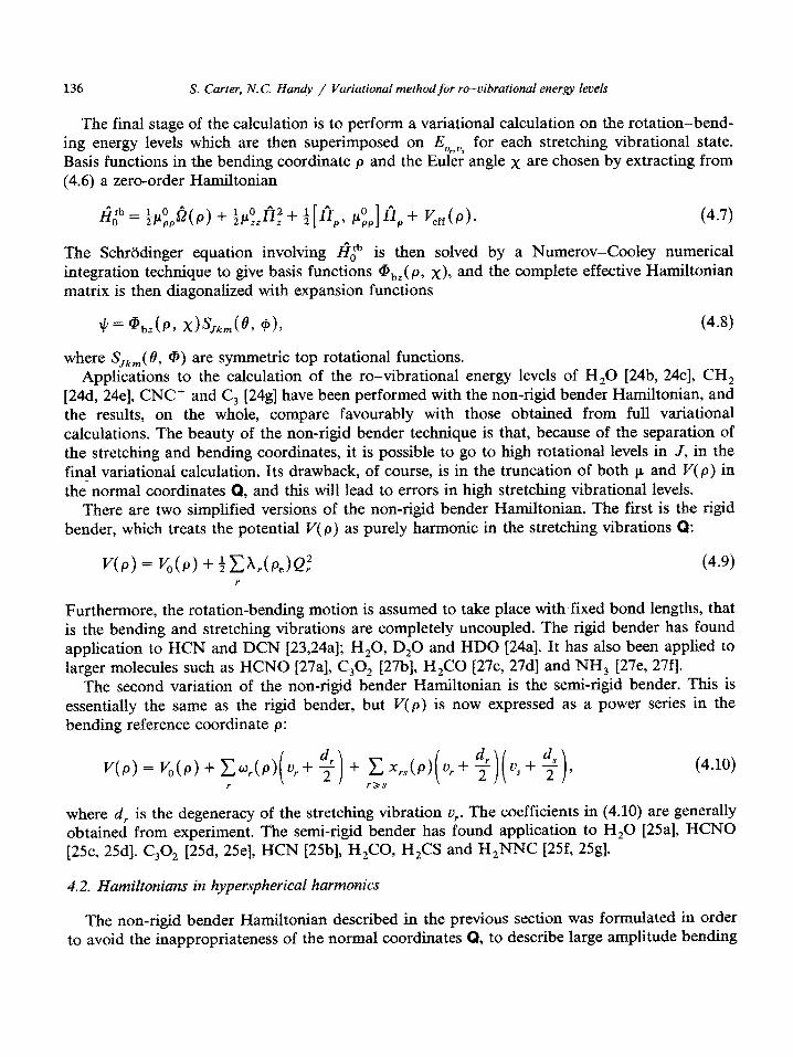
The final stage of the calculation is to perform a variational calculation on the rotation-bend- ing energy levels which are then superimposed on E,,.,, for each stretching vibrational state. Basis functions in the bending coordinate p and the Euler angle x are chosen by extracting from (4.6) a zero-order Hamiltonian
(4.7)
The Schrodinger equation involving fiib is then solved by a Numerov-Cooley numerical integration technique to give basis functions Gbr( p, x), and the complete effective Hamiltonian matrix is then diagonalized with expansion functions
j/ = @br h dsJ,de, (P), (4.8)
where SJk,(O, @) are symmetric top rotational functions. Applications to the calculation of the ro-vibrational energy levels of H,O [24b, 24~1, CH,
[24d, 24e], CNC+ and C, [24g] have been performed with the non-rigid bender Hamiltonian, and the results, on the whole, compare favourably with those obtained from full variational calculations. The beauty of the non-rigid bender technique is that, because of the separation of the stretching and bending coordinates, it is possible to go to high rotational levels in J, in the final variational calculation. Its drawback, of course, is in the truncation of both p and V(p) in the normal coordinates Q, and this will lead to errors in high stretching ~brational levels.
There are two simplified versions of the non-rigid bender Ha~lto~~. The first is the rigid bender, which treats the potential V(p) as purely harmonic in the stretching vibrations Q:
JW = V,(P) + t Chbe>Q: (4.9)
Furthermore, the rotation-bending motion is assumed to take place with fixed bond lengths, that is the bending and stretching vibrations are completely uncoupled. The rigid bender has found application to HCN and DCN [23,24a]; H,O, D,O and HDO [24a]. It has also been applied to larger molecules such as HCNO [27a], C,O, [27b], H,CO [2?c, 27d] and NH, [27e, 27fl.
The second variation of the non-rigid bender Ha~ltonian is the semi-rigid bender, This is essentially the same as the rigid bender, but V(P) is now expressed as a power series in the bending reference coordinate p:
UP)= v,(P)+cw,(P)( u/t; + cx (p) u+3 i- ) r>s rs ( r 2)(uE++)3 (4.10)
where d, is the degeneracy of the stretching vibration u,. The coefficients in (4.10) are generally obtained from experiment. The semi-rigid bender has found application to H,O [25a], HCNO [25c, 25d]. C,O, [25d, 25e], HCN [2Sb], H&O, H,CS and H,NNC [25f, 25g].
The non-rigid bender Hamiltonian described in the previous section was formulated in order to avoid the inappropriateness of the normal coordinates Q, to describe large amplitude bending
S. Carter, N. C. Handy / Eu+iational method for ra-oibrational energy levels 137
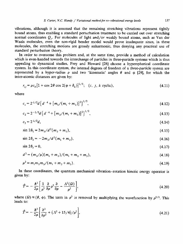
vibrations, although it is assumed that the remaining stretching vibrations represent tightly bound atoms, thus enabling a standard perturbation treatment to be carried out over stretching normal coordinates Q,. For molecules of light and/or weakly bound atoms, such as Van der Waals molecules, even the non-rigid bender model would prove inadequate since, in these molecules, the stretching motions are grossly anh~monic, thus denying any practical use of standard perturbation theory.
In order to overcome this problem and, at the same time, provide a method of calculation which is even-handed towards the interchange of particles in three-particle systems which is thus appealing to dynamical studies, Frey and Howard 1281 choose a hyperspherical coordinate system. In this coordinate system, the internal degrees of freedom of a three-particle system are represented by a hyper-radius p and two ‘kinematic’ angles B and cp [29], for which the inter-atomic distances are given by:
rjj = pc,[l + cos 28 cos 2(+ + 6k)]1’2; (i, j, k cyclic), (4.11)
where
Cl = 2.“Q( d-4 + [ m,/( m, + m2)]2y*,
C~==2-1’ad(6-4+ [“2/(m,+m,)]*)1’2,
(4.12)
(4.13)
c3 = 2-"j2d, (4.14)
sin 25, = 2wr,/d*(m, -+ m,L (4.15)
sin 25, = -2~~/d*~~~ + %)t (4.16)
sin 28, = 0, (4.17)
d2 = bM4( ml + m,Vb, + m2 + m3L (4.18)
# = ~~~*~~/(~~ + *, + *& (4.19)
In these coordinates, the quantum mechanical ~bration-rotation kinetic energy operator is given by:
(4.20)
where (52) = (8, Cp). The term in p5 is removed by multiplying the wavefunction by psj2. This leads to:
&_Az a2 [ 2Y ap2
+ (A2 + 15/4)/p2 , I
(4.21)
138 S. Carter, N.C. Handy / Variational method for ro-vibrational energy levels
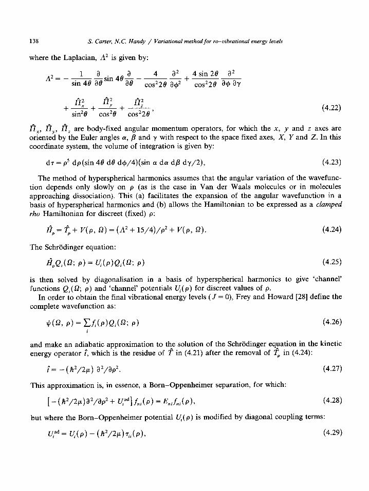
where the Laplacian, A2 is given by:
A2= _L_ a sin 46 ae
+ 4 sin28 a2
c0s22e a+ ay
+ 02 I
0; 0’ sin*8
-+-..-_L_
cos2e c0s22e ’ (4.22)
fiir,, I?,,, I?, are body-fixed angular momentum operators, for which the x, y and z axes are oriented by the Euler angles (Y, p and y with respect to the space fixed axes, X, Y and 2. In this coordinate system, the volume of integration is given by:
dr = p5 dp(sin 48 de d$/4)(sin (Y da dp dy/2), (4.23)
The method of hyperspherical harmonics assumes that the angular variation of the wavefunc- tion depends only slowly on p (as is the case in Van der Waals molecules or in molecules approaching dissociation). This (a) facilitates the expansion of the angular wavefunction in a basis of hyperspherical harmonics and (b) allows the Hamiltonian to be expressed as a clamped rho Hamiltonian for discreet (fixed) p:
fiP=TP+ v(p, 52)=(A2+15/4)/p2+ v(p, i-2).
The Schrijdinger equation:
I-i,Q,@& P) = ~(P)Q;(R P)
(4.24)
(4.25)
is then solved by diagonalisation in a basis of hyperspherical harmonics to give ‘channel’ functions Qj( 9; p) and ‘channel’ potentials Q(p) for discreet values of p.
In order to obtain the final vibrational energy levels (J = 0), Frey and Howard [28] define the complete wavefunction as:
#(a, P) = Cf,(p)Q,(R P) (4.26)
and make an adiabatic approximation to the solution of the Schrodinger equation in the kinetic energy operator ?, which is the residue of f in (4.21) after the removal of fP in (4.24):
t^= - (~2/2~) a2/ap2. (4.27)
This approximation is, in essence, a Born-Oppenheimer separation, for which:
[ -WmWW+ ul~%A~) =~JJP), (4.28)
but where the Born-Oppenheimer potential U;.(p) is modified by diagonal coupling terms:
qad= ~(P)-(A2/2P)Tii(P), (4.29)
S, Carter, N.C. Han& / Variational ~g~hod for ro-vi~rationaI energy levefs 139
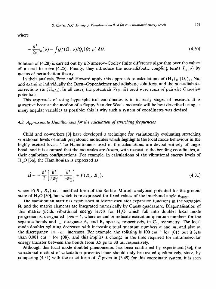
where
- grii(p) = ]Q:(a; p)t^Qi(‘; P) d’* (4.30)
Solution of (4.28) is carried out by a Numerov-Cooley finite difference algorithm over the values of p used to solve (4.25). Finally, they introduce the non-adiabatic coupling terms qj( p) by means of perturbation theory.
In their analysis, Frey and Howard apply this approach to calculations of (H2)3, (D2)2, Ne, and examine indi~dually the horn-Oppe~e~er and adiabatic solutions, and the non-adiabatic corrections (to (H2)3). In all cases, the potentials V{ p, a) used were sums of pairwise Gaussian potentials.
This approach of using hyperspherical coordinates is in its early stages of research. It is attractive because the motion of a floppy Van der Waals molecule will be best described using as many angular variables as possible; this is why such a system of coordinates was devised.
4.3. Approximate Hamiltonians for the calculation of stretching frequencies
Child and co-workers [3] have developed a technique for va~ation~ly evaluating stretching vibrational levels of small polyatomic molecules which ~~~i~ts the local mode behaviour in the highly excited levels. The Hamiltonians used in the calculations are devoid entirely of angle bend, and it is assumed that the molecules are frozen, with respect to the bending coordinates, at their equibrium configurations. For example, in calculations of the vibrational energy levels of H,O [3a], the Hamiltonian is expressed as:
(4.31)
where V( R,, R2) is a modified form of the Sorbie-Mu~ell analytical potential for the ground state of H,O 1301, but which is re-expressed for fixed values of the interbond angle 8,,,.
The hamiltonian matrix is established in Morse oscillator expansion functions in the variables R, and the matrix elements are integrated numerically by Gauss quadrature. Diagonalisation of this matrix yields vibrational energy levels for H,O which fall into doublet local mode progressions, designated 1 nm f ), where m and n indicate excitation quantum numbers for the separate bonds and &- designate A, and B, species, respectively, in C,, symmetry. The local mode doublet splitting decreases with increasing total quantum numbers n and m, and also as the discrepancy 1 n - m 1 increases. For example, the splitting is 100 cm-i for 101) but is less than 0.001 cm-i for ]OS), and this implies a change in the time required for intramolecular energy transfer between the bonds from 0.5 ps to 30 ns, respectively.
Although this local mode doublet phenomenon has been confirmed by experiment (3e], the variational method of calculation presented here should only be treated qu~itatively, since, by comparing (4.31) with the exact form of T given in (3.49) for this coordinate system, it is seen
140
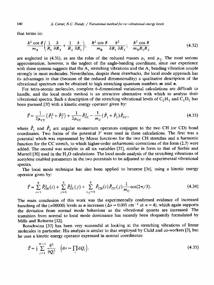
that terms in:
S. Carter, N. C. Handy / Variational method for ro-vibrational energy levels
a2 tr2 cos 8 -- lJR,ilR,' m,R,R,
(4.32)
are neglected in (4.31), as are the roles of the reduced masses pl and ,u2. The most serious approximation, however, is the neglect of the angle-bending coordinate, since our experience with these systems suggests that the A, stretching vibrations and the A, bending vibration couple strongly in most molecules. Nevertheless, despite these drawbacks, the local mode approach has its advantages in that (because of the reduced dimensionality) a qualitative description of the vibrational spectrum can be obtained to high stretching quantum numbers m and n.
For tetra-atomic molecules, complete &dimensional variational calculations are difficult to handle, and the local mode method is an attractive alternative with which to analyse their vibrational spectra. Such a description of the stretching vibrational levels of C,H, and C,D, has been pursued f3fl with a kinetic energy operator given by:
(4.33)
where fir and F2 are angular momentum operators conjugate to the two CH (or CD) bond coordinates. Two forms of the potential V were used in these calculations. The first was a potential which was represented by Morse functions for the two CH stretches and a harmonic function for the CC stretch, to which higher-order anharmonic corrections of the form (2.3) were added. The second was analytic in all six variables [31], similar in form to that of Sorbie and Murrell[30] used in the H,O calculations. The local mode analysis of the stretching vibrations of acetylene enabled parameters in the two potentials to be adjusted to the experimental vibrational spectra.
The local mode technique has also been applied to benzene [3e], using a kinetic energy operator given by:
The main conclusion of this work was the expe~menta~y confirmed evidence of increased bunc~ng of the (~~) levels as n increases (Av = 0.001 cm-’ at n = 4), which again supports the deviation from normal mode behaviour as the vibrational quanta are increased. The transition from normal to local mode dominance has recently been eloquently formulated by Mills and Robiette [32].
(4.34)
Botschwina [33] has been very successful at looking at the stretching vibrations of linear molecules in particular. His analysis is similar to that employed by Child and co-workers [3], but he uses a kinetic energy operator expressed in normal coordinates:
(4.35)
S. Carter, N.C. Ham” / Variational ~eth~~vr r5-vibrational energy levels
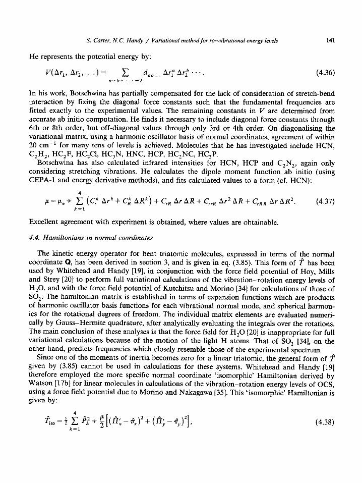
He represents the potential energy by:
141
V(Ar,, At-,, . . . )= c do,.,. ArpAr,b-a-. (4.36) a+b+ . . . -2
In his work, Botschwina has partially compensated for the lack of consideration of stretch-bend interaction by fixing the diagonal force constants such that the fundamental frequencies are fitted exactly to the experimental values. The remaining constants in V are determined from accurate ab initio computation. He finds it necessary to include diagonal force constants through 6th or 8th order, but off-diagonal values through only 3rd or 4th order. On diagonalising the variational matrix, using a harmonic oscillator basis of normal coordinates, a~eement of within 20 cm-’ for many tens of levels is achieved. Molecules that he has investigated include HCN, C,H,, HC,F, HC,Cl, HC,N, HNC, HCP, HC,NC, HC,P.
Botschwina has also calculated infrared intensities for HCN, HCP and C,N,, again only considering stretching vibrations. He calculates the dipole moment function ab-initio CEPA-1 and energy derivative methods), and fits calculated values to a form (cf. HCN):
4
p=pe+ C (C/‘ Ark+ Ck ARk) + C,, Ar AR + CrrR Ar2 AR + C,, Ar AR=. (4.37)
(using
k=l
Excellent agreement with experiment is obtained, where values are obtainable.
4.4. ~a~i~~an~ans in normal coordinates
The kinetic energy operator for bent triatomic molecules, expressed in terms of the normal coordinate Q, has been derived in section 3, and is given in eq. (3.85). This form of f has been used by Whitehead and Handy [19], in conjunction with the force field potential of Hoy, Mills and Strey [20] to perform full variational calculations of the vibration-rotation energy levels of H&I, and with the force field potential of Kutchitsu and Morino [34] for calculations of those of SO,. The hamiltonian matrix is established in terms of expansion functions which are products of harmonic oscillator basis functions for each vibrational normal mode, and spherical harmon- ics for the rotational degrees of freedom. The indi~du~ matrix elements are evaluated numeri- cally by gauss-Her~te quadrature, after ~~ytically evaluating the integrals over the rotations. The main conclusion of these analyses is that the force field for H,O 1201 is inappropriate for full variational calculations because of the motion of the light H atoms. That of SO, [34], on the other hand, predicts frequencies which closely resemble those of the experimental spectrum.
Since one of the moments of inertia becomes zero for a linear triatomic, the general form of f given by (3.85) cannot be used in calculations for these systems. Whitehead and Handy [19] therefore employed the more specific normal coordinate ‘isomorphic’ Hamiltonian derived by Watson [17b] for linear molecules in calculations of the vibration-rotation energy levels of OCS, using a force field potential due to Morino and Nakagawa [35]. This ‘isomorphic’ Hamiltonian is given by:
(4.38)
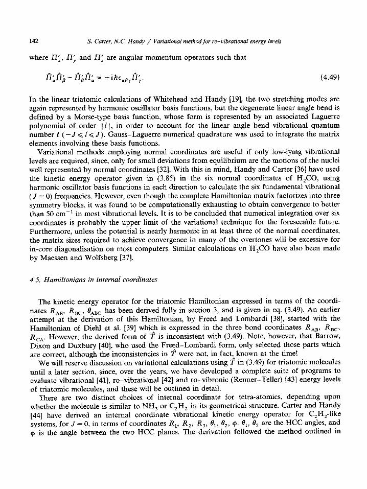
142 S. Carter, N.C. Handy / Variational method for ro-oibra~io~a~ energy levels
where II:, WY and II: are angular momentum operators such that
(4.49)
In the linear triatomic calculations of Whitehead and Handy [19], the two stretching modes are again represented by harmonic oscillator basis functions, but the degenerate linear angle bend is defined by a Morse-type basis function, whose form is represented by an associated Laguerre polynomial of order 1 f I, in order to account for the linear angle bend vibrational quantum number I (-J G f G J). Gauss-Laguerre numerical quadrature was used to integrate the matrix elements involving these basis functions.
Variational methods employing normal coordinates are useful if only low-lying vibrational levels are required, since, only for small deviations from equilibrium are the motions of the nuclei well represented by normal coordinates [32]. With this in mind, Handy and Carter [36] have used the kinetic energy operator given in (3.85) in the six normal coordinates of H&O, using harmonic oscillator basis functions in each direction to calculate the six fundamental vibrational (J = 0) frequencies. However, even though the complete Hamiltonian matrix factorizes into three symmetry blocks, it was found to be computationally exhausting to obtain convergence to better than 50 cm-’ in most vibrational levels. It is to be concluded that numerical integration over six coordinates is probably the upper limit of the variational technique for the foreseeable future. Furthermore, unless the potential is nearly harmonic in at least three of the normal coordinates, the matrix sizes required to achieve convergence in many of the overtones will be excessive for in-core diagonalisation on most computers. Similar calculations on H,CO have also been made by Maessen and Wolfsberg [37].
4.5. Hamiltonians in internal coordinates
The kinetic energy operator for the triatomic Hamiltonian expressed in terms of the coordi- nates RAB, -RBC, flABc has been derived fully in section 3, and is given in eq. (3.49). An earlier attempt at the derivation of this Ha~ltonian, by Freed and Lombardi [38], started with the Hamiltonian of Diehl et al. [39] which is expressed in the three bond coordinates RAB, RBc, R CA. However, the derived form of f is inconsistent with (3.49). Note, however, that Barrow, Dixon and Duxbury [40], who used the Freed-Lombardi form, only selected those parts which are correct, althou~ the inconsistencies in f were not, in fact, known at the time!
We will reserve discussion on variational calculations using !I? in (3.49) for triatomic molecules until a later section, since, over the years, we have developed a complete suite of programs to evaluate vibrational [41], ro-vibrational [42] and ro-vibronic (Renner-Teller) [43] energy levels of triatomic molecules, and these will be outlined in detail.
There are two distinct choices of internal coordinate for tetra-atomics, depending upon whether the molecule is similar to NH, or C,H, in its geometrical structure. Carter and Handy [44] have derived an internal coordinate vibrational kinetic energy operator for C,H,-like systems, for J = 0, in terms of coordinates R,, R *, R,, 8,, S,, $. i& 0, are the HCC angles, and # is the angle between the two HCC planes. The derivation followed the method outlined in
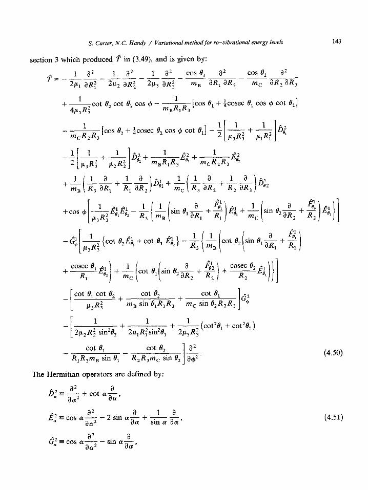
S. Carter, N. C. Handy / Variational method for ro-vibrational energy Ievels 143
section 3 which produced f in (3.49), and is given by:
1 a2 I a2 1 a2 cos 8, a2 ~=_______--__-
cos 0, a2 -_ 3% aR,2 2k aR; 53% aR; mB aR, aR, in, aR, aR,
1 f- 4PL,R: cot 6, cot 0, cos 4 - m B ; 13 R [cos 8, + t+osec 8, cos + cot &]
- nz i R [cos O,+ icosec 02 cos cp cot 8J - $
c 2 3
+cos $I
cot 8, cot 62 +
cot e2 +
cot 6, -
P3G m, sin e1R,R3 m, sin O,R,R,
I
6;
1 - 2~ 2 R$ sin’@,
+ 1 t1 2~IR~sin261
- (cot28, + cot%J 2P&
cot 8, cot 6, a2 - R,R,m, sin B1 - l- R,R,m, sin 8, a@’
The Hermitian operators are defined by:
a2 ii,“=- a
aa -i-cot (Ya(y,
a2 _?+cos cy-- 3+__ I a
aff2 2 sin (Y acu
since aar’
(4.50)
(4.51)
a2 +cos(Y-- a
aa sin ixz,
144 S. Carter, N.C. Handy / Variational method for ro-vibrational energy levels
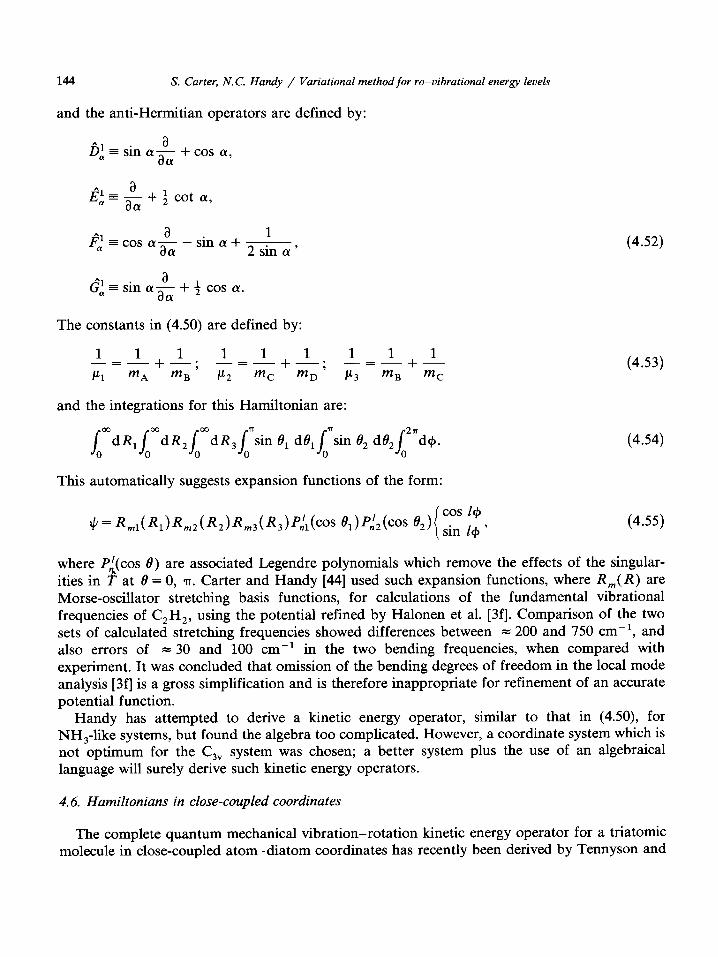
and the anti-Hermitian operators are defined by:
1 F~=cosn$-sina+-.
2 sin (Y ’
The constants in (4.50) are defined by:
1 1 1 -=-++---’ E”1 mA mB
9 1 1 1 1 1 1
-_=-+-. -=_+_ p2 mC mD ’ c13 mB mC
and the integrations for this Hamiltonian are:
This automatically suggests expansion functions of the form:
(4.52)
(4.53)
(4.54)
(4.55)
where Pk(cos 0) are associated Legendre polynomials which remove the effects of the singular- ities in T at 8 = 0, 71. Carter and Handy [44] used such expansion functions, where R,(R) are Morse-oscillator stretching basis functions, for calculations of the fundamental vibrational frequencies of C,H,, using the potential refined by Halonen et al. [3fl. Comparison of the two sets of calculated stretching frequencies showed differences between = 200 and 750 cm-‘, and also errors of = 30 and 100 cm-’ in the two bending frequencies, when compared with experiment. It was concluded that omission of the bending degrees of freedom in the local mode analysis [3fl is a gross simplification and is therefore inappropriate for refinement of an accurate potential function.
Handy has attempted to derive a kinetic energy operator, similar to that in (4.50), for NH,-like systems, but found the algebra too complicated. However, a coordinate system which is not optimum for the C,, system was chosen; a better system plus the use of an algebraical language will surely derive such kinetic energy operators.
4.6. Hamiltonians in close-coupled coordinates
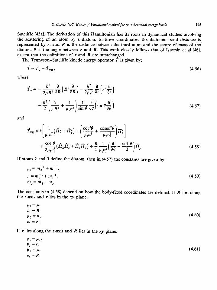
The complete quantum mechanical vibration-rotation kinetic energy operator for a triatomic molecule in close-coupled atom-diatom coordinates has recently been derived by Tennyson and
S. Carter, N. C. Handy / Variational method for ro-vibrational energy levels 145
Sutcliffe [45a]. The derivation of this Hamiltonian has its roots in dynamical studies involving the scattering of an atom by a diatom. In these coordinates, the diatomic bond distance is represented by r, and Ii is the distance between the third atom and the centre of mass of the diatom. 8 is the angle between IC and R. This work closely follows that of Istomin et al [46], except that the definitions of r and R are interchanged.
The Tennyson-Sutcliffe kinetic energy operator ? is given by:
i:= fv -I- fVR,
where
and
(4.56)
(4.57)
(4.58)
If atoms 2 and 3 define the diatom, then in (4.57) the constants are given by:
y, = rn;l+ m;l,
p = m;’ + my’, mj=m2+m,.
(4.59)
The constants in (4.58) depend on how the body-fixed coordinates are defined. If R lies along the z-axis and r lies in the xy plane:
Pl ==PY
v1 = R
Y2 = Pj9
v2 = r.
If r lies along the z-axis and R lies in the xy plane:
Pl = Pj,
u1 = r,
!42=EL,
u,=R.
(4.60)
(4.61)
146 S. Carter, N.C. Handy / Variationai method for ro-vibrational energy levels
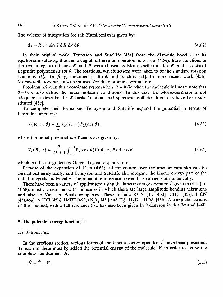
The volume of integration for this Hamiltonian is given by:
dr = R2r2 sin @ dR dr d8. (4.62)
In their original work, Tennyson and Sutcliffe [45a] froze the diatomic bond r at its equilibrium value r,,, thus removing all differential operators in r from (4.56). Basis functions in the remaining coordinates R and 8 were chosen as Morse-oscillators for R and associated Legendre polynomials for 8. The rotational wavefunctions were taken to be the standard rotation functions D;cU, (a, 8, y) d escribed in Brink and Satchler [21]. In more recent work [45b], Morse-oscillators have also been used for the diatomic coordinate r.
Problems arise, in this coordinate system when R = 0 (ie when the molecule is linear; note that B = 0, ?I also define the linear molecule conditions). In this case, the Morse-oscillator is not adequate to describe the R basis function, and spherical oscillator functions have been sub- stituted [45cf.
To complete their formalism, Tennyson and Sutcliffe expand the potential in terms of Legendre functions:
V(R, r, 0) = ~V,(R, +‘,(cos O), (4.63) x
where the radial potential coefficients are given by:
VA@, f-1 = &/+‘P,(cos B)V(R, r, 8) d cos 8 -1
which can be integrated by Gauss-Legendre quadrature. Because of the expansion of Y in (4.63), all integration over the angular variables can be
carried out analytically, and Tennyson and Sutcliffe also integrate the kinetic energy part of the radial integrals analytically. The remaining integration over ‘v is carried out n_umerically.
There have been a variety of applications using the kinetic energy operator T given in (4.56) to (4.58), mostly concerned with molecules in which there are large amplitude bending vibrations and also to Van der Waals complexes. These include KCN [45a, 45d], CH: [45e], LiCN [45f,45g], ArHCl[45h], HeHF [45i], (N2)2 [45j] and H3+, H,DS, HD; f45k]. A complete account of this method, with a full reference list, has also been given by Tennyson in this Journal [461].
5. The potential energy function, Y
5.1. Introduction
In the previous section, various forms of the kinetic energy operator ? have been presented. To each of these must b,e added the potential energy of the molecule, V, in order to derive the complete hamiltonian, H:
rzi=?+v. (5.1)
S. Carter, N. C. Handy / Variational method for m-vibrational energy levels 147
In all but a very few cases, V will be given by the Born-Oppenheimer potential, that is, coupling between the nuclear and electronics motions will be neglected. The exception to this will be if a study of Renner-Teller systems is required, in which case the electronic orbital angular momentum operator L becomes important where surfaces of differing symmetries become degenerate.
As we have seen, once the coordinate system required to tackle a particular problem has been chosen, it is now a straightforward (albeit somewhat tedious) task to derive the appropriate form of i?: This is always given in closed analytical form, and is valid over the entire coordinate space. It is a different matter altogether to decide upon the form of V to be used in (5.1), always assuming, of course, that information is known about Y in the first place! By definition, the potential will have to be appropriate to those regions of the surface that are represented by minima (the stable configurations), and there may be more than one of these on the potential surface. It may be required to investigate these minima in~~dually in order to evaluate the vibrational energy levels for each configuration in turn, in which case individual potentials V will be required to represent such minimum. On the other hand, one may wish to investigate tunnelling between the several minima, and this will require a single potential V which encompasses all minima and the saddle points that connect them. Finally, vibrational energy levels close to dissociation may be required, for example in the study of reaction dynamics, and this demands yet a different form of V.
5.2. Ab initio potentials
The source of potential energy surfaces relevant to the vibration-rotation variational problem is, convention~y, spectroscopy. In this case, functions forms of V in terms of the internal (or normal) coordinates of the indi~dual minima, whose spectra have been recorded, are (some- times) available. However, these are known accurately for only a few molecules. In the absence of any experimental data on the molecular potential energy surface, the only way to obtain I’ is via ab initio calculation. It is now routine to obtain grids of ab initio energies for any specified geometries of the molecule in any required set of coordinates. If this is the case, then all elements in the variational hamiltonian matrix must be integrated numerically. The problem here is to decide at which points on the surface to calculate the ab initio energies. If the numerical integration technique is (say) Gauss quadrature, then for a set of integration points M, it is possible to pre-determine the geometries of the molecule which correspond to these integration points (there will be M1 X M, X M3 of them for a triatomic molecule). Bartholamae, Martin and Sutcliffe [47] have used this technique to determine at which points to evaluate ab initio energies for CH:.
One of the hazards of numerical integration, however, is that an initial selection of integration points M may not be sufficient to exactly integrate over V, and increasing numbers of points M’
will usually have to be tried until convergence is reached. Furthermore, if the number of basis functions !Dr needs to be increased in order to obtain convergence in the energy levels with respect to the basis size, this will correspondingly lead to an increase in the number of integration points M in order to integrate over @; and thus maintain exact integration over I’. This means that the initial grid of ab initio energies will now not be precisely on the integration points, and the energies will either have to be re-calculated at the new points, or interpolated by some fitting procedure. Either method is tedious and undesirable.
148 S. Carter, N.C. Ham” / Variational method for ro-v~br~tionaS energy ievels
5.3. Fore field potentials
It is now possible to calculate derivatives of the potential by ab initio methods, and if these derivatives are calculated at the minimum of the potential, a function V in the form if (2.3) or (4.1) can be derived. This is the form of V conventionally presented by the spectroscopist. Providing that only the vibrational energy levels of a single minimum are required, then these ‘force-field’ potentials are, in principle, adequate. Even so, if one wishes to evaluate vibrational levels other than those that lie close to the minimum of the potential well, these force field potentials will not, in all but a few exceptions, contain derivatives of sufficiently high order to bring about convergence to the true energy levels (there are rarely sufficient spectroscopic data to evaluate force constants to higher than quartic (and usually not even sufficient data to derive a complete quartic force field, even for triatomic molecules) and it is not yet possible to determine high-order force constants ab initio to any degree of accuracy).
Improved force fields can be obtained however by transforming the force constants given in (2.3) to Simons-Parr-Finlan coordinates [ll], whereupon improved convergence is achieved over the bond stretches. The potential over the bond angles Bi, however, is still problematic since, if the molecule becomes linear as any ei + 71, the potential must have the property (aV/W,)?r = 0 and this property is difficult to achieve with force fields of the form of (2.3) and impossible with those of the form (4.1). For potentials with large barriers to linearity (e.g. H,O) this is not usually a serious problem, but for molecules with low barriers to linearity (eg CH,I) it is vital. Also, it is not possible to represent V in the form of (2.3) or (4.1) to describe a surface with multiple minima.
One point in favour of force field potentials, however, is their simplicity, which usually means that it is possible to integrate the matrix elements involving Y analytically. Indeed one pre-requisite of the non-rigid bender approach [26] is that V is expressed in the form of (4.1) solely for this purpose. This factor makes the Taylor expansion of V an ideal ‘model’ potential with which to test new kinetic energy operators T, or new types of expansion function Qr,, but it is not sufficiently flexible for serious variational calculations unless the higher-order constants can be determined, for example, as has Botschwina [33] by refining them directly to the observed vibrational spectrum.
The form of the potential ir to be used in the variational calculations is, to a large extent, dictated by the problem to be tackled and , to a lesser extent, by, the form of the expansion functions Gr which are themselves governed by the choice of T. Some workers (ourselves included) direct their research towards the refinement of complete potential energy surfaces via the variational technique, and this work demands that V is as accurate as possible over large regions of coordinate space. This implies that integrations of the matrix elements in variational calculations involving such potentials will inevitably be carried out numerically, and so the actual form of V is irrelevant (although it is desirable to be able to compute the potential efficiently for any given geometry). This type of potential, however, must be carefully contrived. Other workers (cf. Child ]3] and Botschwina [33]) are content to use model potentials, usually of the force field variety, in order to facilitate analytical inte~a~on of the matrix elements. As both of these authors have found, some ‘tidying up’ of these potentials (e.g. refinement to the spectra of high-order terms) is necessary in order to regain the accuracy lost due to their limited range.
S. Carter, N.C. Handy / Variational method for ro-vibrational energy levels 149
These authors have also found it necessary to omit the awkward bending coordinate from their calculations. It ought to be said at this stage, however, that unless the proposed analysis demands the inclusion of a complicated potential, there is ~~~~Z~~e~y no need to resort to any but the simplest possible form of V.
To summarize therefore, the problem to be investigated dictates the coordinate system and hence the form of f to be used in the variational calculations, and these, in turn, lead to the optimum choice of basis function (sp, which comes closest to diagonalise f. Only when these have been selected should the potential V, of minimum complexity to complete the analysis, be sought.
The foregoing is intended to alert the reader to the possible dilemmas that he may face when undertaking variational calculations for small polyatomic molecules, since the cccuracy of his results will ultimately depend on the accuracy of Y (all kinetic energy operators T are equivalent in their respective coordinate systems). Even though kinetic energy operators can be derived for any molecule, of any size, in any coordinate system, it is an unfortunate fact that reliable potentials are known for only a very few (usually triatomic) molecules, and there are barely a handful known for tetra-atomic molecules. Furthermore, the dimensionahty of the tetra-atomic problem forbids much serious work (involving full variational treatments) on these systems at the moment, and it is therefore to be anticipated that, for the immediate future, most complete variational analyses will be conducted for triatomic molecules.So far in this section, we have discussed potentials V that can be obtained from ab initio calculations in the form of energy grids, and from ab initio calculations and/or spectroscopy in the form of Taylor expansion force fields. We have also made the reader aware of the dangers of using both types of potential. We now go on to discuss other forms of Y that have found use in variational calculations.
Over a decade ago, a functional form of V known as the LEPS (London [48], Eyring, Polanyi [49], Sato [50]) potential had become very popular in the study of reaction dynamics. Recently, Connor and Clary [51] have used such a potential in variational calculations on the repulsive surface of IHI. This is dominated by a collinear saddle point which is bound with respect to the dissociation products HI + I only by virtue of zero point energy, there being a maximum in the potential along the collinear reaction coordinate.
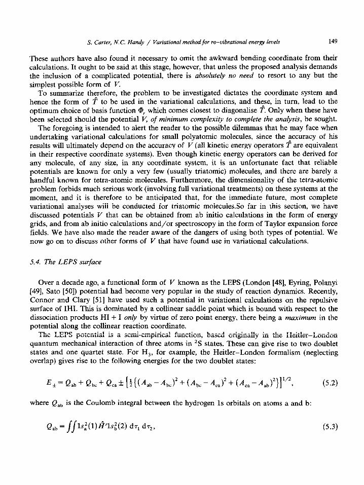
The LEPS potential is a semi-empirical function, based originally in the Heitler-London quantum mechanical interaction of three atoms in 2S states. These can give rise to two doublet states and one quartet state. For II,, for example, the Heitler-London formalism (neglecting overlap) gives rise to the following energies for the two doublet states:
where Qat, is the Coulomb integral between the hydrogen 1s orbitals on atoms a and b:
(5.2)
(5.3)
150 S. Carter, N. C. Handy / Variational method for ro-vibrational energy levels
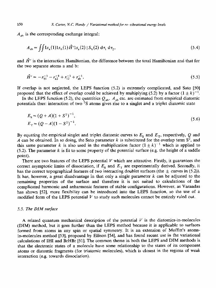
A,, is the corresponding exchange integral:
4J = JJ l~,(l)ls,,(l)fi’ls,(2) 1 S,(2) dr, dr2, (5.4)
and fi’ is the interaction Hamiltonian, the difference between the total Hamiltonian and that for the two separate atoms a and b:
(5.5)
If overlap is not neglected, the LEPS function (5.2) is extremely complicated, and Sato [50] proposed that the effect of overlap could be achieved by multiplying (5.2) by a factor (1 It k)-l.
In the LEPS function (5.2), the quantities eat,, A, etc. are estimated from empirical diatomic potentials thus: interaction of two 2S atoms gives rise to a singlet and a triplet diatomic state
Es = (Q + A)(1 + S2)-l,
E, = (Q - A)(1 - S2)-‘. (5.6)
By equating the empirical singlet and triplet diatomic curves to Es and E,, respectively, Q and A can be obtained. In so doing, the Sato parameter k is substituted for the overlap term S2, and this same parameter k is also used in the multiplication factor (1 + k)-’ which is applied to (5.2). The parameter k is fit to some property of the potential surface (e.g. the height of a saddle point).
There are two features of the LEPS potential v which are attractive. Firstly, it guarantees the correct asymptotic limits of dissociation, if Es and E, are experimentally derived. Secondly, it has the correct topographical features of two interacting doublet surfaces (the + curves in (5.2)). It has, however, a great disadvantage in that only a single parameter k can be adjusted to the remaining properties of the surface and therefore it is not suited to calculations of the complicated harmonic and anharmonic features of stable configurations. However, as Varandas has shown [52], more flexibility can be introduced into the LEPS function, so the use of a modified form of the LEPS potential V to study such molecules cannot be entirely ruled out.
5.5. The DIM surface
A related quantum mechanical description of the potential T/ is the diatomics-in-molecules (DIM) method, but it goes further than the LEPS method because it is applicable to surfaces formed from atoms in any spin or spatial symmetry. It is an extension of Moffitt’s atoms- in-molecules method [53], proposed by Ellison [54], and has found recent use in the variational calculations of IHI and BrHBr [51]. The common theme in both the LEPS and DIM methods is that the electronic states of a molecule have some relationship to the states of its component atoms or diatomic fragments (for triatomic molecules), which is closest in the regions of weak interaction (e.g. towards dissociation).
S. Carter, N.C. Handy / Variational method for ro-vibrational energy levels 151
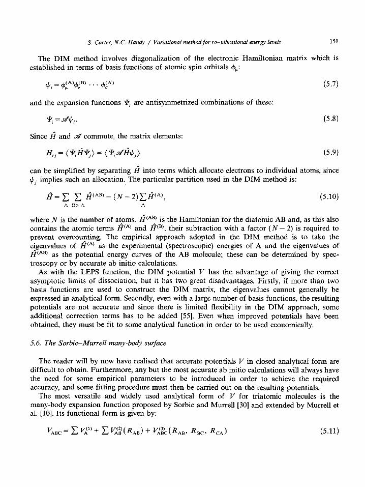
The DIM method involves diagonalization of the electronic Hamiltonian matrix which is established in terms of basis functions of atomic spin orbitals #p:
(5 3
and the expansion functions $ are antisymmetrized combinations of these:
14: =.?Z&.
Since g and & commute, the matrix elements:
(5 4
(5 *9)
can be simplified by separating fi into terms which allocate electrons to individual atoms, since \tj implies such an allocation. The particular partition used in the DIM method is:
&C C &AB)- (~-2)j-‘@4), (5.10) A BbA A
where N is the number of atoms. aCAB) is the Hamiltonian for the diatomic AB and, as this also contains the atomic terms tiCA) and &B), their subtraction with a factor (N - 2) is required to prevent over-counting. The empirical approach adopted in the DIM method is to take the eigenvalues of AtA) as the experimental (spectroscopic) energies of A and the eigenvalues of ACAB) as the potential energy curves of the AB molecule; these can be determined by spec- troscopy or by accurate ab initio calculations.
As with the LEPS function, the DIM potential I’ has the advantage of giving the correct asymptotic limits of dissociation, but it has two great disadvantages. Firstly, if more than two basis functions are used to construct the DIM matrix, the eigenvalues cannot generally be expressed in analytical form. Secondly, even with a large number of basis functions, the resulting potentials are not accurate and since there is limited flexibility in the DIM approach, some additional correction terms has to be added [55]. Even when improved potentials have been obtained, they must be fit to some analytical function in order to be used economically,
The reader will by now have realised that accurate potentiafs V in closed analytical form are difficult to obtain. Furthermore, any but the most accurate ab initio calculations will always have the need for some empirical parameters to be introduced in order to achieve the required accuracy, and some fitting procedure must then be carried out on the resulting potentials,
The most versatile and widely used analytical form of V for triatomic molecules is the many-body expansion function proposed by Sorbie and Murrell[30] and extended by Murrell et al. {lo]. Its functional form is given by:
V ABC = c&i"+ C%?@AB)+ 'l;&@AB, RBC, &A) (5.11)
152 S. Carter, N.C. Handy / Variational method for ro-vibrational energy levels
There are certain similarities between this and the DIM method in that the potentials vjl), the atomic energies, and V’g( R,,), the diatomic terms, are both included in V,,, and can be taken from the experimental (spectroscopic) quantities. Unlike the DIM method, however, only those Vdl) and v&)( R,,) which appear in the dissociation schemes of the state of the triatomic under investigation are required.
The two-body terms Vdg(R,,) are derived from spectroscopic or ab initio data in the form of extended Rydberg potentials [56]:
Yc2)(li) = -D,(l + Crp + C,p2 + C3p3) exp( -yp), (5.12)
where p = R - R, (R, is the equilibrium bond length) and D, is the dissociation energy of the diatom. The constants Ci and y are fit to the spectroscopic force constants or to accurate ab initio energies.
The three-body term V$& (R,, R,,, RCA) is then fit to the remaining triatomic features of the potential, such as harmonic and anharmonic force constants of stable configurations. It is written in the form:
Vo( Rj) = I’( R,)T( Ri), (5.13)
where P( Rj) is a general polynomial in the bond distances R, and T( Ri) is a range function which goes to zero as any bond distances Ri becomes infinite. Because of this, it can be seen, from (5.12) and (5.13) that the potential V (5.11) has the correct dissociation limits providing that the -Y(r) and V(*)(R) are exact, The form of T( Ri) is given by
T(Ri) = ,lfIl [l - t4YjS,/2)],
with
(5.14)
(5.15)
pi being taken from some suitable reference Ry (pi = Ri - Ry). The parameters yj in (5.14) are adjustable, and for any selection of these, the coefficients in the polynormal I’( Ri) are determined from the triatomic data.
This form of Y has found application to a wide range of triatomic molecules and is particularly convenient for variational calculations. The general aspects of (5.11) are discussed in detail in ref. [lo], and the variational applications will be discussed in the following section.
5.7. Van der Waals potentials
The many-body expansion potential (5.11) is ideal for investigating ti~tly-bound molecules, since there is a linear relationship relating the force constants to the coefficients of P( Ri). However, it does not, as yet, include the correct long-range features which are relevant to the study of weakly bound Van der Waals minima, although these are currently being investigated 1571.
S. Curter, N.C. Handy / Variational method for ro-vibrational energy 2eueis 153
Historically, the binding energies of Van der Waals molecules are best represented in terms of a multi-polar expansion [%I. For a diatom& molecule, this gives rise to a long-range potential V of the form:
V(R) = - (C6R-6 + C,R_” + C,,R-lo + - * - ), (5.16)
where the constants C,, C,, C,, are related to the multipoles of the diatom by perturbation theory, providing that overlap can be neglected. If overlap cannot be neglected, the C,, coefficients become functions of R and it is customary to include the effect of overlap by introducing some damping function D, ( R ) :
C,*(R) = C,D,(R). (5.17)
This form of V has lost favour for polyatomic molecules, since it is very slowly convergent. For these triatomic systems, there are a variety of potentials Y in use, but we will discuss only
two of them. The first has been used extensively by Hutson and Howard [59] and assumes that the potential to be constructed is relevant for an atom-rigid diatom system. It is given in the form:
VCR, 8) = @)( -&x-‘- -&x-$
where
x = R’R,@h n = r@(e) + y(x - 1).
In (5.18) and (5.19), B is the scattering angle, and:
e(O) =e(O") + Aqf(B; X) + Ae2g(6)),
R,(B) = R,@=) + A%@; k) + AQ@),
m(s) = m(CP) + Amf(8; 6).
where
f(@; A) = 1 - [$(1+ cos X)l^.
(5.18)
(5.19)
(5.20)
(5.21)
The function g( 8) is defined by
g(8) = cos28 (e > 900),
0) = 0 (e < 900). (5.22)
The expressions for the potential defined by (5.18) to (5.22) contains twelve parameters which Hutson and Howard fit to the spectroscopic data for the inert gas-HCl complexes 1.591.
ut ua@ J, ‘pm?y laylo ayl UQ *S~XT! 3t2auf1 aql lnoqt! uo~~~~lo~ dq passac0~ ifIpi?twf? a3~ sa3nlcKk3ls
asayl Sil?a>aq~ ‘(lt c 0 pug LL > 8) -etufu~ ,wapAtnba, uaaMK?q wa33a %UffIaUUnl p~?f3gpn? m 03 spEa1 snl~, *ur ut?yl 3ajsa32i sr 8 a@w puoq ayj '13~~ ~03 sa3nlDn3R UT sljnsa3 salsufp300:, puuou ayl30 a3nlau 3eaur1ya3 aye sr! ‘(s~-E)u~ ua~f%~ %ufsn sarwQnba33 %tupuaq ~~auo~ aye uyqo 01
afqfssodurf sf $f ‘lu!od ajpp~?s 3eauf1 ay$ aaoqa ai1 sla~a~ %cupuaq3o 6lyo@u ayl a3ay~ ‘sajn~alow
,3vauy-fswnb, asayl 303 ‘leyl papnpuo3 ah '(~~‘#T)uI.Io~ 3eaurI ayl 8ufsn (LIMOIS hraa) pa%3aAuoD
k;ayl l'i?yl Inq‘(S8'~)ux303 iuaq ay, %utsn sfsEq %ursea39ur y~f~ pa83aAfp slaAa1 pi?uorle3q?A 5knpuaq
ayl 1Byl "[t? la at?uroIoy~3e~ pfp SB ‘puno~ pw 's3ow3ado k83aua 3pauyy s,uos~%?~ 30 ~~1303 3eauy
puv luaq ayl ytoq %UySn suo~l~~n3~e~ p~.Ioy?p~~ Ino pa&LIeD 9~. ‘lylualod sgl ~lr& .[Ig] l_m3
1~6 aq 01 3afuEq ST% pavTpa3d put? ‘sahIn3 +EO~IXJJ +HD put! Z~ If?luar.upadxa %ufsn (~f's)
two3 Ieuo~3un3 e 01 t?lep asaql 1;~ aM ‘[up] '$a3 UT &3 303 slufod w?p oypl qt! aq %ufsfi ‘IL = 8 $12 iiq.n?p%~~s I? sq (sg*gj wyl ~23 ayl ~JIM paIdno
‘tC1!3EaufI 0% 3ap3Eq puxs kw.np.3oe3~xa aq 03 sq painqyw pug ‘azfs sy2q aql UT asea3;7ur
ue 01 vadsar yzf~ wa%3aArl, a3aM sa'ceds ST% 30 SU@~JO pwq uy3ac1l~?yl‘(~8*~)%u~sn ‘pun03 [t@]
aJj~i2lns pun up3e~4 ‘avruo~oy~3v~ ‘f$3 30 sIaAa1 1woyc-Tq:A aql 30 sfs1cp2ut? ut? UI *saInDaIour
(8f'p) 3eauTI 30 (58.c) tuaq 303 s3ola3ado Braua 3yauy apour 1?2tu3ou s,uos~afi %ufsn ‘[61]
~puej~ put? p%?aqalyMiCq padolanap asoyl a3aM poqlaw p~?uoy~?+rt?~ayl dqsaIn~a,aIouIc)fuIow~3130
SIaAaI 1C%3aua uo~lt?lo3-uoyE?~q~A %UgI?tIIEAa 303 pasn AIapfM 1sou.1 sw&o3d aql ‘@IaDa IrJun
fog] pal-eIn3p2D meads lfayl pur! (SF?% alay E x) X+-I 303 pauft?lqo uaaq aA??y (92-s) 0% &Z'S)
Aq uaA:s pyuawd ayl uy srawunwd *"' uofwny atp JO ~n~~~ aql 30 uorltsod aql ST mx
(9Z’S) ‘rk < 8) I = wa ‘(?I 3 8) ,[I - (x/wx))P-]dxa = (@a
Aq uan@ sr ((~~*g)aas) (8)~ uoyun3 %ufdrut?p ayl a3ayM
(KS) ‘
[&L&l + ,-&,‘3](zf)Q - (~V-)dxa yyY= (2pA
:dq uaA$ asf! suoy2unJ ptpa3 ay& -d puf! 8 uaahilaq a@he
ay$ S_I 0 pwe suotvun3 ajpua%al a.~ (0 SOD)~~ *uxol~~p ayl30 wauraDeIds!p ssaIuoyw.np ayl st
(KS) od/(“.f-d) =$
pue ‘.f puoq +.uowp ayl30 a3luaD put! ~301~ aq~ uaahlaq a2ur2lsIp ayl SF 8 a3ay~
Z‘O=Y O=Y
(EZ’S) ‘(xyA(6 soqya,s 3 1 = (6 ‘3 ‘x).4
:dq uaA@ SF 11 *~~MOIIE SF tuoisfp aqi 30 uogmqy ~DTM 303 lnq ‘saletup300~
uxo~rr~p-Mona UT [og] -1~ Ia Lox a? Ilq pasn auo st uo ww_w.uo~ a& @puatod puoDas aq&
S. Carter, N.C. Handy / Variational method for ro-vibrational energy levels 155
(4.38) leads, ultimately, to the correct bending levels, but in this case, the rectilinear nature of the bending coordinate now prohibits access to regions around the potential minimum during the integration procedure, unless either the minimum lies close to 8 = T or an enormous number of basis functions and integration points are used.
6.1. The vibrational (J = 0) programs JEQO, JEQOT, JEQOS, JEQOST [62]
From the above analysis, it is apparent that normal coordinates cannot be used to investigate vibrational levels of floppy triatomics, and this prompted us [41] to design a new variational procedure based on the J = 0 kinetic energy operator fv given in (3.49) in terms of the two bond lengths R,, R, and the included angle 6’ (it is worth mentioning that fv in_(3.49) can be obtained, as well as by the method outlmed in section 3, by applying a similarity transformation (sin 0)-‘/2T(sin 0) ‘I2 to the operator T given by Carney, Sprandel and Kern [S]). This operator fv is Hermitian in the sense that:
(6.1)
and also there are no difficulties when the molecule is linear, in contrast to Watson’s normal coordinate operator (3.85), because (sin 0 fv) does not have a singularity at 8 = 0, T.
Our original program was JEQO, which commences by selecting the appropriate basis functions +,, to be used in the variational expansion functions @:
@(n,, n2, 4 = ~~,,(R,)~~*(R,)~~,,(e). (6.2)
The variational eigenfunctions ‘k, are obtained by diagonalization of the Hamiltonian matrix set up in these orthonormal product expansion functions @:
W% n2, n,)= C pjk
,. @cni> njy nk) (6.3) i,j,k
for which the individual Hamiltonian matrix elements
~mdRr~OCdR2~ 8 de @(ni, nj, nk)gv@(n:, n;, ni) 64
are calculated numerically using m,, m2, me ( = m,) Gauss-quadrature integration points, respectively. We will now discuss the derivation of the basis functions +n for JEQO before introducing the refinements included in the remaining programs.
6.2. Vibrational basis functions
For each of the three variables p = R,, R 2, 8 the selection of the appropriate basis function &,( p) depends on certain factors. Firstly, the number ~tl, and the positions q,, of integration points for each coordinate p must be known. The former is input into the program as a
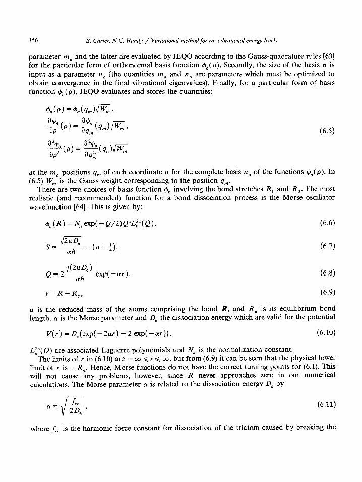
156 S. Curter, N.C. Handy / Variational method for ro-vibrational energy levels
parameter mP and the latter are evaluated by JEQO according to the Gauss-quadrature rules 1631 for the particular form of orthonormal basis function c&(p). Secondly, the size of the basis n is input as a parameter n, (the quantities M, and n, are parameters which must be optimized to obtain convergence in ihe final vibrationa\ eigenvalues). Finally, for a particular form of basis function c#+,( p), JEQO evaluates and stores the quantities:
(6.5)
at the mP positions 4, of each coordinate p for the complete basis nP of the functions (p,(p). Jn (6.5) ;W;, is the Gauss weight corresponding to the position q,.
There are two choices of basis function C& involving the bond stretches R, and R,. The most realistic (and recommended) function for a bond dissociation process is the Morse oscillator wavefunction [64]. This is given by:
(P,(R) = N, ew(-QP)Q”~?(Q),
s._ @ix _(n+l) -- ah 2 f
Q=2_exp(-ar) fxpl ,
r=R-Re,
(6.6)
(6.7)
(6.8)
(6.9)
p is the reduced mass of the atoms comprising the bond A?, and R, is its equilibrium bond length. a: is the Morse parameter and 0, the dissociation energy which are valid for the potential
V(Y) =DJexp( -2ar) - 2 exp( -ffr)), (6.10)
I,:$( Q) are associated Laguerre polyno~als and N, is the normalization constant. The limits of r in (6.10) are - co < r G a, but from (6.9) it can be seen that the physical lower
limit of r is -R,. Hence, Morse functions do not have the correct turning points for (6.1). This will not cause any problems, however, since R never approaches zero in our numerical calculations. The Morse parameter (Y is related to the dissociation energy 0, by:
LX= (6.11)
where f,, is the harmonic force constant for dissociation of the triatom caused by breaking the
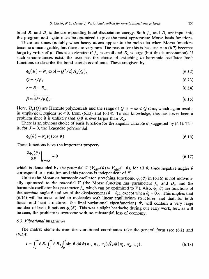
S. Carter, N. C. Handy / Variational method for ro-vibrational energy levels 157
bond R, and De is the co~espon~ng bond dissociation energy. Both f,, and De are input into the program and again must be optimized to give the most appropriate Morse basis functions.
There are times (notably when heavy atoms appear in the molecule) when Morse functions become unmanageable, but these are very rare. The reason for this is because s in (6.7) becomes large by virtue of p. This is accelerated if f,, is small and 0, is large (but this is uncommon). If such circumstances exist, the user has the choice of switching to harmonic oscillator basis functions to describe the bond stretch coordinate. These are given by:
%@I = N, exp(-Q2/2)WQ),
Q = r/P,
r=R-R,,
(6.12)
(6.13)
(6.14)
P=@iz (6.15)
Here, H,(Q) are Hermite polynomials and the range of Q is - co < Q < 00, which again results in unphysical regions R < 0, from (6.13) and (6.14). To our knowledge, this has never been a problem since it is unlikely that Qp is ever larger than R,.
There is an obvious choice of basis function for the angular variable 0, suggested by (6.1). This is, for J = 0, the Legendre polynomial:
(p,(e) = N,$(cos et
These functions have the important property
(6.16)
(6.17)
which is demanded by the potential Y ( VABC( 8) = V,,,( - 8), for all 8, since negative angles 8 correspond to a rotation and this process is independent of 8).
Unlike the Morse or harmonic oscillator stretching functions, rp,(8) in (6.16) is not individu- ally optimized to the potential Y (the Morse function has parameters f,, and De, and the harmonic oscillator has parameter f,, which can be optimized to V). Also, $I~(@) are functions of the Q~~~~~~e angle B and not of the displacement (8 - S,), except when 8, = 0,~. This implies that (6.16) will be most suited to molecules with linear equilib~um structures, and that, for both linear and bent structures, the final variational eigenfunctions 9r will contain a very large number of basis functions cP,(S). This was a slight headache during our early work, but, as will be seen, the problem is overcome with no substantial loss of economy.’
6.3. Vibrational integration
The matrix elements over the vibrational coordinates take the general form (see (6.1) and (6.2)):
(6.18)
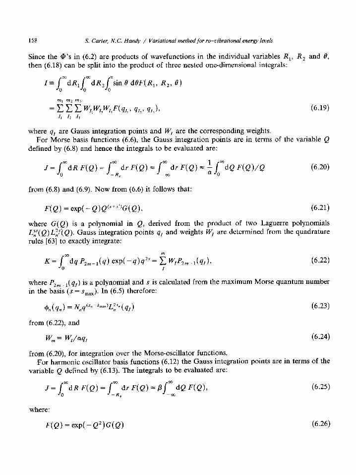
158 S. Carter, N.C. Handy / Variational method for ro-vibrational energy levels
Since the @‘s in (6.2) are products of wavefunctions in the individual variables R,, R, and 8, then (6.18) can be split into the product of three nested one-dimensional integrals:
(6.19)
where qr are Gauss integration points and WI are the corresponding weights. For Morse basis functions (6.6), the Gauss integration points are in terms of the variable Q
defined by (6.8) and hence the integrals to be evaluated are:
J=JmdRF(Q)=jm 0 -R,
drF(Q)=jm drF(Q)=$=dQF(Q)/Q --Do
(6.20)
from (6.8) and (6.9). Now from (6.6) it follows that:
F(Q) = exp( - Q>Q(s's')G(Q>, (6.21)
where G(Q) is a polynomial in Q, derived from the product of two Laguerre polynomials Ls;‘( Q)Lz:‘(Q). Gauss integration points q1 and weights WI are determined from the quadrature rules [63] to exactly integrate:
K= J m&l P,,-,(q) exPk7)q2" = 2 w,p,,_,(q,), 0 I
(6.22)
where ‘*m- I( 41) is a polynomial and s is calculated from the maximum Morse quantum number
in the basis (s = s,,). In (6.5) therefore:
(6.23)
from (6.22), and
wm = W,h7, (6.24)
from (6.20), for integration over the Morse-oscillator functions. For harmonic oscillator basis functions (6.12) the Gauss integration points are in terms of the
variable Q defined by (6.13). The integrals to be evaluated are:
J = imdR F(Q) = I_; dr f’(Q) = Plm dQ F(Q), e --cc,
(6.25)
where:
r;(Q) = exp( - Q')G(Q) (6.26)
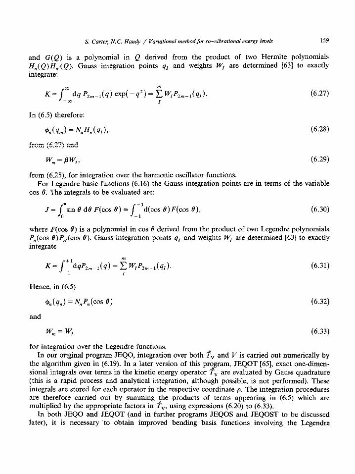
S. Curter, N. C. Hundy / Variational method for ro-vibrational energy levels 159
and G(Q) is a polynomial in e derived from the product of two Hermite polynomials
~~(~}~~/(Q). G auss integration points q1 and weights IV1 are determined [63] to exactly integrate:
K= J 43 dq %dd exd -q2) = E W,4,-,(q,h (6.27)
--00 I
In (6.5) therefore:
(6.28)
from (6.27) and
cy;, = Pw;, (6.29)
from (6.25), for integration over the harmonic oscillator functions. For Legendre basic functions (6.16) the Gauss integration points are in terms of the variable
cos 8. The integrals to be evaluated are:
J = Jo”sin 8 de F(cos 0) = /_l’d(cos B)F(cos 0), (6.30)
where F(cos 0) is a polynomial in cos @ derived from the product of two Legendre polynomials P,(cos @)P,,(cos 0). Gauss integration points qr and weights Cyr are determined [63] to exactly integrate
(6.31)
Hence, in (6.5)
(6.32)
and
wm = wr
for integration over the Legendre functions.
(6.33)
In our original program JEQO, integration over both fv and V is carried out numerically by the algorithm given in (6.19). In a later version of this pr?gram, JEQOT [65], exact one-dimen- sional integrals over terms in the kinetic energy operator Tv are evaluated by Gauss quadrature (this is a rapid process and analytical integration, although possible, is not performed). These integrals are stored for each operator in the respective coordinate p. The integration procedures are therefore carried out by summing the products of terms appearing in (6.5) which are multiplied by the appropriate factors in I’v, using expressions (6.20) to (6.33).
In both JEQO and JEQOT (and in further programs JEQOS and JEQOST to be discussed later), it is necessary to obtain improved bending basis functions involving the Legendre
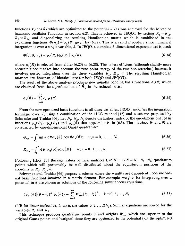
160 S. Carter, N. C. Handy / Variational method for ro-vibrational energy levels
functions P,(cos 8) which are optimized to the potential V (as was achieved for the Morse or harmonic oscillator functions in section 6.2). This is achieved in JEQOT by setting R, = RI,, R, = R,, and diagona~zing the resulting Ha~ltonian matrix which is established in the expansion functions @(n,) = cP,,( 8) given by (6.32). This is a rapid procedure since numerical integration is over a single variable, 8. In JEQO, a complete 3-dimensional expansion set is used:
where (g,(R) is selected from either (6.23) or (6.28). This is less efficient (although slightly more accurate since it takes into account the zero point energy of the two bon stretches) because it involves nested integration over the three variables R,, R,, 8. The resulting Hamiltonian matrices are, however, of identical size for both JEQO and JEQOT).
The result of the above analysis produces new angular bending basis functions 4,(B) which are obtained from the eigenfunctions of fiv in the reduced basis:
(6.35) i-0
From the now optimized basis functions in all three variables, JEQOT modifies the integration technique over V, using a combination of the HEG method [15] and a scheme proposed by Schwenke and Truhlar 1663. Let A$, A& N3 denote the highest index of the one-dimensional basis functions +#,), %z(&) and q,,(S) that appear in !I$ in (6.3). The matrices 0 and R are constructed by one-dimensional Gauss quadrature:
s,,,=J*sinedtt~,ie)coss~,(e); m,n=0,1,...,N3, 0
(6.36)
R = mn J ma %,g(R)Wn(R); m,n = 0, I,..., iv. (6.37) 0
Following HEG [15], the eigenvalues of these matrices give iV + 1 (N = N,, A$, N3) quadrature points which will presumably be well distributed about the equilibrium positions of the coordinates R,, R,, 8.
Schwenke and Truhlar 1661 propose a scheme where the weights are dependent upon individ- ual basis functions involved in a matrix element. For example, weights for inte~ating over a potential in 8 are chosen as solutions of the following simultaneous equations:
k=O, l,...,N, (6.38) l=O
(NB for linear molecules, k takes the values 0, 2,. . . , 2N,). Similar equations are solved for the variables R, and R,.
This technique produces quadrature points 4 and weights Wkn which are superior to the original Gauss points and ‘weights’ since they are optimized to the potential (via the optimized
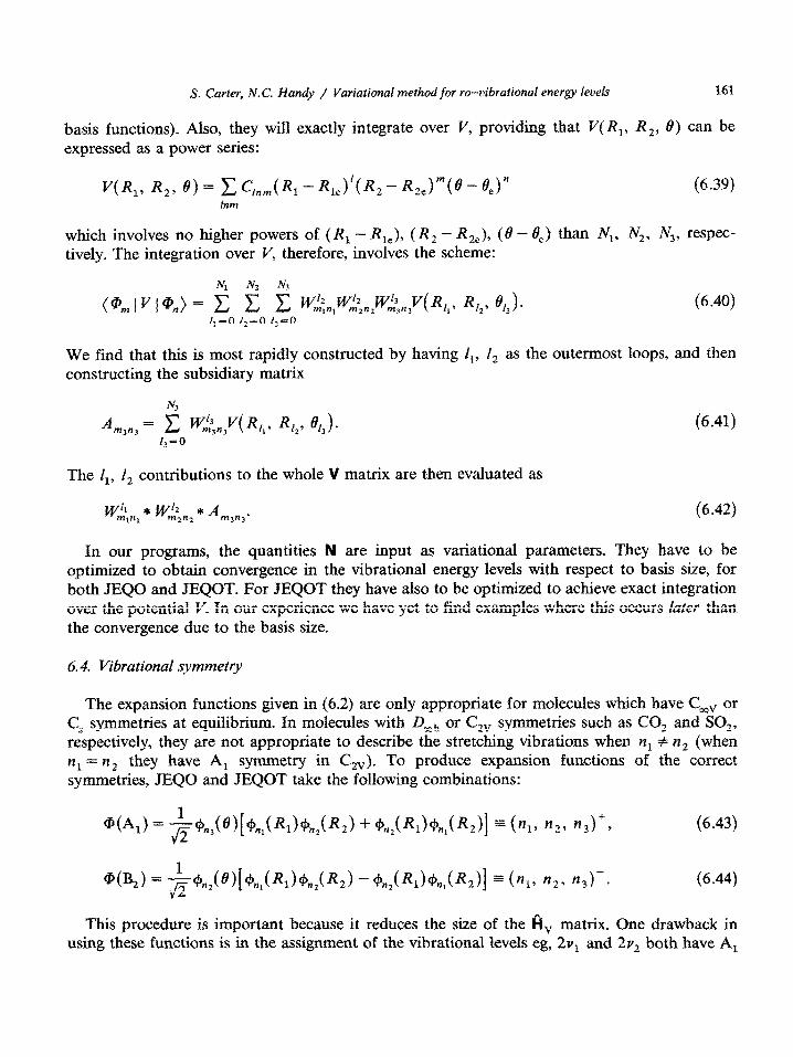
S. Carter, N.C. Handy / Variational method for ro-vibrational energy ievels 161
basis functions)_ Also, they will exactly integrate over V, providing that V(R,, R,, 0) can be expressed as a power series:
(6.39)
which involves no higher powers of (R, - Ri,), (R, - RZe), (B - 0,> than N,, N2, N3, respec- tively. The integration over V, therefore, involves the scheme:
We find that this is most rapidly constructed by having I,, t, as the outermost loops, and then constructing the subsidiary matrix
(6.41)
The I,, I, contributions to the whole V matrix are then evaluated as
In our programs, the quantities N are input as variational parameters. They have to be optimized to obtain convergence in the vibrational energy levels with respect to basis size, for both JEQO and JEQOT. For JEQOT they have also to be optimized to achieve exact integration over the potential V. In our experience we have yet to find examples where this occurs later than the convergence due to the basis size.
6.4. Vibrational symmetry
The expansion functions given in (6.2) are only appropriate for molecules which have C,, or C, sy~et~es at equilib~um. In molecules with Beoh or C,, s~met~es such as CO, and SO,, respectively, they are not appropriate to describe the stretching vibrations when n, f: n2 (when 82, = n2 they have A, symmetry in C,,). To produce expansion functions of the correct symmetries, JEQO and JEQOT take the following combinations:
(6.43)
(6.44)
This procedure is important because it reduces the size of the A, matrix. One drawback in using these functions is in the assignment of the vibrational levels eg, 2v, and 2v, both have A,
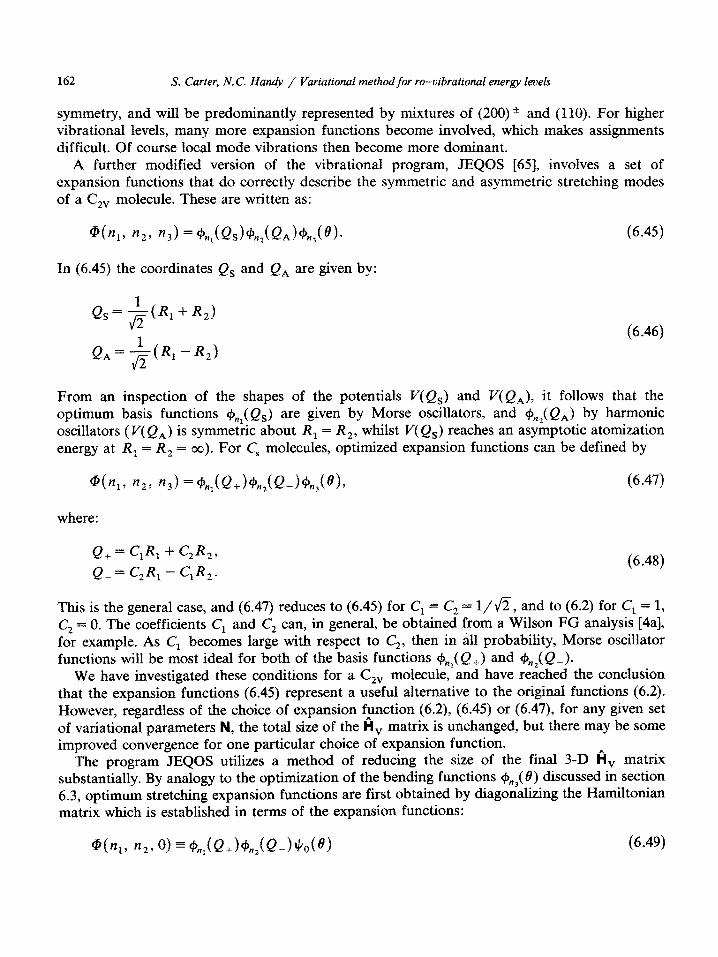
162 S. Carter, N.C. Handy / Variational method for ro-vibrational energy leveis
symmetry, and will be predominantly represented by mixtures of (200) * and (110). For higher vibrational levels, many more expansion functions become involved, which makes assignments difficult. Of course local mode vibrations then become more dominant.
A further modified version of the vibrational program, JEQOS [65], involves a set of expansion functions that do correctly describe the symmetric and asymmetric stretching modes of a C,, molecule. These are written as:
In (6.45) the coordinates Q, and QA are given by:
Q,=-$R,+R,)
Q,=+-R,)
(6.46)
From an inspection of the shapes of the potentials V(Q,) and V( QA), it follows that the optimum basis functions $$ Q,) are given by Morse oscillators, and &,,( QA) by harmonic oscillators (V( QA) is s y mmetric about R, = R,, whilst V( Q,) reaches an asymptotic atomization energy at R, = R, = co). For C, molecules, optimized expansion functions can be defined by
@(n,, n2, n3) = ~~,(Q+)~,,(Q-)#~,(6), (6.47)
where:
Q, = C,R, + C,R,, Q_ = C,R, - C,R,.
(6.48)
This is the general case, and (6.47) reduces to (6.45) for C, = C, = l/a, and to (6.2) for C, = 1, C, = 0. The coefficients C, and C, can, in general, be obtained from a Wilson FG analysis [4a], for example. As C, becomes large with respect to C,, then in all probability, Morse oscillator functions will be most ideal for both of the basis functions cp,,(Q+) and cp,,(Q_).
We have investigated these conditions for a C, molecule, and have reached the conclusion that the expansion functions (6.45) represent a useful alternative to the original functions (6.2). However, regardless of the choice of expansion f:nction (6.2), (6.45) or (6.47), for any given set of variational parameters N, the total size of the H, matrix is unchanged, but there may be some improved convergence for one particular choice of expansion function.
The program JEQOS utilizes a method of reducing the size of the final 3-D Hv matrix substantially. By analogy to the optimization of the bending functions &( 8) discussed in section 6.3, optimum stretching expansion functions are first obtained by diagonalizing the Hamiltonian matrix which is established in terms of the expansion functions:
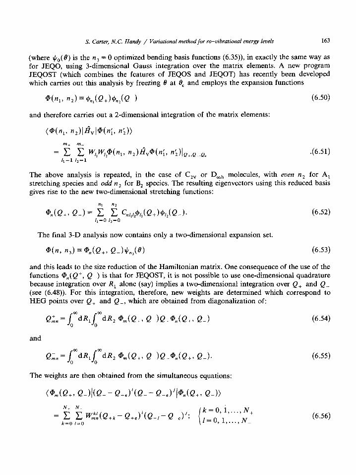
S. Carter, N. C. Handy / Variational method for ro-vibrational energy levels 163
(where GO( 0) is the n3 = 0 optimized bending basis functions (6.35)), in exactly the same way as for JEQO, using 3-dimensional Gauss integration over the matrix elements. A new program JEQOST (which combines the features of JEQOS and JEQOT) has recently been developed which carries out this analysis by freezing 19 at 19, and employs the expansion functions
@(n,, n2) = +n,,,(Q+h,,(Q-) (6.50)
and therefore carries out a 2-dimensional integration of the matrix elements:
.(6.51) I,=1 I*=1
The above analysis is repeated, in the case of C, or Dmh molecules, with euen n2 for A, stretching species and odd n2 for B, species. The resulting eigenvectors using this reduced basis gives rise to the new two-dimensional stretching functions:
@n(Q+, Q-> = 2 ? c,,,,,~,,(Q+>~,,(Q->. (6.52) I,=0 lz=O
The final 3-D analysis now contains only a two-dimensional expansion set.
@i(n, n3) = @n(Q+, Q-)4@> (6.53)
and this leads to the size reduction of the Hamiltonian matrix. One consequence of the use of the functions Qn( Q+, Q-) is that for JEQOST, it is not possible to use one-dimensional quadrature because integration over R, alone (say) implies a two-dimensional integration over Q, and Q_ (see (6.48)). For this integration, therefore, new weights are determined which correspond to HEG points over Q, and Q_, which are obtained from diagonalization of:
Q;, = ~mdRl~mdR, @,(Q+, Q-)Q+@n(Q+, Q-1
and
Q,, = J,k~ mdR, @,JQ+, Q-)Q-@n(Q+, Q-h
The weights are then obtained from the simultaneous equations:
(@,(Q+, Q-)l(Q+ - Q+,>‘(Q- - Q-e)'(@n(Q+> Q-j>
N, N-
= c c JT,kf,(Q+, - k=O I=0
Q+Ji(Q_,- Q-,)'; { ;~;‘1”‘**‘,“+ , ,..., _
(6.54)
(6.55)
(6.56)
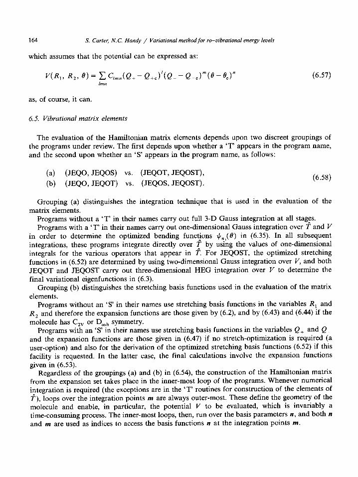
164 S. Carter, N. C. Handy / Variational method for ro-vibrational energy levels
which assumes that the potential can be expressed as:
V(R,, R,, f’) = c C,,,(Q+ - Q+,)‘(Q- - Q-e)“@ - 8)” Imn
(6.57)
as, of course, it can.
6.5. Vibrational matrix elements
The evaluation of the Hamiltonian matrix elements depends upon two discreet groupings of the programs under review. The first depends upon whether a ‘T’ appears in the program name, and the second upon whether an ‘S’ appears in the program name, as follows:
(a) (JEQO, JEQos) VS. (JEQOT, JEQOST) ,
(b) (JEQO, JEQOT) VS. (JEQoS, JEQOST). (6.58)
Grouping (a) distinguishes the integration technique that is used in the evaluation of the matrix elements.
Programs without a ‘T’ in their names carry out full 3-D Gauss integration at all stag_es. Programs with a ‘T’ in their names carry out one-dimensional Gauss integration over T and V
in order to determine the optimized bending functions #,,(fl) in (6.35). In all subsequent integrations, these programs integrate directly over ? by using the values of one-dimensional integrals for the various operators that appear in i? For JEQOST, the optimized stretching functions in (6.52) are determined by using two-dimensional Gauss integration over V, and both JEQOT and JEQOST carry out three-dimensional HEG integration over V to determine the final variational eigenfunctions in (6.3).
Grouping (b) distinguishes the stretching basis functions used in the evaluation of the matrix elements.
Programs without an ‘s’ in their names use stretching basis functions in the variables R, and R, and therefore the expansion functions are those given by (6.2), and by (6.43) and (6.44) if the molecule has C,, or Dooh symmetry.
Programs with an ‘S’ in their names use stretching basis functions in the variables Q, and Q_ and the expansion functions are those given in (6.47) if no stretch-optimization is required (a user-option) and also for the derivation of the optimized stretching basis functions (6.52) if this facility is requested. In the latter case, the final calculations involve the expansion functions given in (6.53).
Regardless of the groupings (a) and (b) in (6.54), the construction of the Hamiltonian matrix from the expansion set takes place in the inner-most loop of the programs. Whenever numerical integration is required (the exceptions are in the ‘T’ routines for construction of the elements of f), loops over the integration points m are always outer-most. These define the geometry of the molecule and enable, in particular, the potential V to be evaluated, which is invariably a time-consuming process. The inner-most loops, then, run over the basis parameters n, and both n and m are used as indices to access the basis functions n at the integration points m.
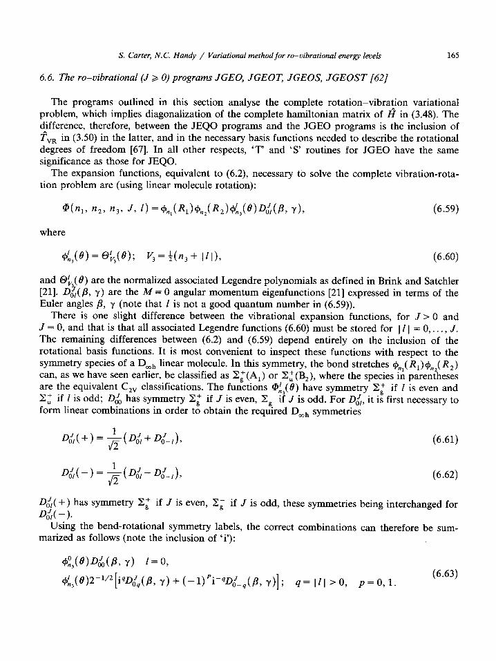
S. Carter, N.C. Handy / Variational method for ro-vibrational energy levels
6.6. The ro-vibrational (J >, 0) programs JGEO, JGEOT, JGEOS, JGEOST [62]
165
The programs outlined in this section analyse the complete rotation-vibration variational problem, which implies diagonalization of the complete hamiltonian matrix of I? in (3.48). The efference, therefore, between the JEQO programs and the JGEO programs is the inclusion of TVR in (3.50) in the latter, and in the necessary basis functions needed to describe the rotational degrees of freedom [67]. In all other respects, ‘T’ and ‘s’ routines for JGEO have the same significance as those for JEQO.
The expansion functions, equivalent to (6.2), necessary to solve the complete vibration-rota- tion problem are (using linear molecule rotation):
&,V) = @&(e>; v, = 3(n, + I l I>, (6.60)
and Ot,( 0) are the normalized associated Legendre polynomials as defined in Brink and Satchler
1211. Qm VI are the it4 = 0 angular momentum eigenfunctions [21] expressed in terms of the Euler angles j3, y (note that I is not a good quantum number in (6.59)).
There is one slight difference between the vibrational expansion functions, for J > 0 and J = 0, and that is that all associated Legendre functions (6.60) must be stored for 111 = 0,. . . , J.
The remaining differences between (6.2) and (6.59) depend entirely on the inclusion of the rotational basis functions. It is most convenient to inspect these functions with respect to the symmetry species of a Dmh linear molecule. In this symmetry, the bond stretches G~,,( Rl)+nZ( R2) can, as we have seen earlier, be classified as Zi(A,) or Zz(B,), where the species in parentheses are the equivalent C,, classifications. The functions @L3(8) have symmetry Xg’ if 1 is even and Zz if 1 is odd; D& has symmetry 29’ if J is even, Xg if J is odd. For D& it is first necessary to form linear combinations in order to obtain the required Doch symmetries
D&( +) has symmetry 29’
D&(-X
if J is even, 2; if J is odd, these symmetries
Using the bend-rotational symmetry labels, the correct combinations marized as follows (note the inclusion of ‘i’):
+!#)2-‘/‘liqD&(P, Y) + (-1)‘ip4QL(P, v)l; q= Ill > 0,
(6.61)
(6.62)
being interchanged for
can therefore be sum-
p=o, 1. (6.63)
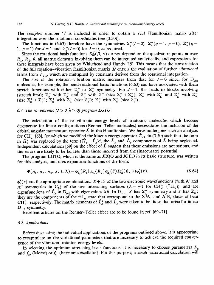
166 S. Carter, N.C. Handy / Variational method~~r r~-vibra~~v~a~ energy levels
The copnpZex number ‘i’ is included in order to obtain a real Hamiltonian matrix after integration over the rotational coordinates (see (3.50)).
The functions in (6.63) therefore have the symmetries Z;(I = 0), 2,‘(4 = 1, p = 0), Z;( q = 1, p = 1) for J = 1 and Z,‘( I = 0) for J = 0, as required.
Since the rotational basis functions O&(/3, y) do not depend on the quadrature points m over R,, R,, 6, all matrix elements involving them can be integrated analytically, and expressions for these integrals have been given by Whitehead and Handy 1191. This means that the construction of the full rotation-vibration Hamiltonian matrix fi entails the evaluation of further vibrationat terms from fvR, which are multiplied by constants derived from the rotational integration.
The size of the rotation-~bration matrix increases from that for J = 0 since, for I>,, molecules, for example, the bend-rotations basis functions (6.63) can have associated with them stretch functions with either 2: or 2,’ symmetry. For J = 1, this leads to blocks involving (stretch first); 22: with 2; and 2: with 2; (size x:g’ + 22:); 22: with 2; and Z:p’ with 2; (size 2:p’ + Z:); 2g’ with Zf (size 2:); 2: with 2: (size 2,‘).
6.7. The ro-vibronic (J 2 0, X > 0) program LGTO
The calculation of the ro-vibronic energy levels of triatomic molecules which become degenerate for linear configurations (Renner-Teller molecules) necessitates the inclusion of the orbital angular momentum operator e in the H~lto~~. We h%ve undergone such an analysis for CH; 1681, for which we modified the_tietie en,ergy opezator TVR in (3.50) _such that the term in fii was replaced by the term (II, + L,)*, the Lx and I;v components of L being neglected. Independent calculations 1691 on the effect of L suggest that these omissions are not serious, and the errors are likely to be far less than those incurred from the (inaccurate) potential.
The program LGTO, which is the same as JEQO and JGEO in its basic structure, was written for this analysis, and uses expansion functions of the form:
(6.64)
&(r) are the appropriate combinations X f iY of the two electronic wavefunctions (with A’ and A” symmetries in-C,) of the two interacting surfaces (h = + 1 for CH: ( 21’IU)), and are eigenfunctions of L, in Dmh with eigenvalues Xtr. In Doct,, X has 2: sy~et~ and Y has 2;; they are the components of the 211, state that corrzspond to the X*A, and A2B, states of bent CH: , respectively. The matrix elements of i,’ and L, were taken to be those that arise for linear Dmh symmetry.
Excellent articles on the Renner-Teller effect are to be found in ref. [69-711.
6.8. Applications
Before discussing the individual applications of the programs outlined above, it is appropriate to recapitulate on the variational parameters that are necessary to achieve the required conver- gence of the ~bration-rotation energy levels.
In selecting the optimum stretching basis functions, it is necessary to choose parameters Be and f,, (Morse) or f,, (harmonic oscillator)_ For this purpose, a smaZ1 variational calculation will
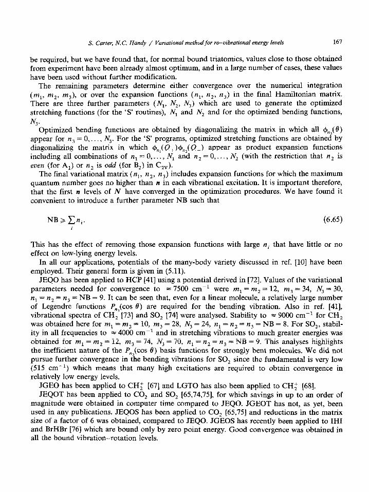
S. Carter, N.C. Handy / Variational ~et~~~ar ro-u~brationa~ energy levels 167
be required, but we have found that, for normal bound triatomics, values close to those obtained from experiment have been already almost optimum, and in a large number of cases, these values have been used without further modification.
The remaining parameters determine either convergence over the numerical integration
(m,, m2, m,), or over the expansion functions (n,, n2, ~1~) in the final Hamiltonian matrix. There are three further parameters (lv,, N2, &) which are used to generate the optimized stretching functions (for the ‘S’ routines), Ni and iV.. and for the optimized bending functions,
% Optimized bending functions are obt~ned by ~agonali~ng the matrix in which all r&,,(e)
appear for n3=0,_.., N3. For the ‘S’ programs, optimized stretching functions are obtained by diagonalizing the matrix in which $I~~( e+)+,,(&) appear as product expansion functions including all combinations of n, = 0,. . . , Nl and n 2 = 0,. . . , A$ (with the restriction that n2 is even (for A,) or n2 is odd (for B,) in C,).
The final variational matrix (n,, n 2, ns) includes expansion functions for which the maximum quantum number goes no higher than n in each vibrational excitation. It is important therefore, that the first n levels of N have converged in the optimization procedures. We have found it convenient to introduce a further parameter NB such that
This has the effect of removing those expansion functions with large nj that have little or no effect on low-lying energy levels.
In all our applications, potentials of the many-body variety discussed in ref. [lo] have been employed. Their general form is given in (5.11).
JEQO has been applied to HCP [41] using a potential derived in [72]. Values of the variational parameters needed for convergence to ~7500 cm-’ were m1=m2=12, m,=34, Nj=30,
- = NB = 9. It can be seen that, even for a linear molecule, a relatively large number $ ~~~e~~:k functions P (cos 6) are required for the bending vibration. Also in ref. [41], vibrational spectra of CH”,3 1731 and SO, [74] were analysed. Stability to = 9000 cm-l for CH, was obtained here for m, = m2 = 10, m3 = 28, N3 = 24, n, = n2 = n3 = NB = 8. For SO,, stabil- ity in all frequencies to = 4000 cm-’ and in stretching vibrations to much greater energies was obtained for m, = m2 = 12, rn3 = 74, N3 = 70, ~zi = n2 = n3 = NB = 9. This analyses highlights the inefficient nature of the P,,(cos 6) basis functions for strongly bent molecules, We did not pursue further convergence in the bending vibrations for SO, since the fundamental is very low (515 cm-‘) which means that many high excitations are required to obtain convergence in relatively low energy levels.
JGEO has been applied to CH: [67] and LGTO has also been applied to CH; [68]. JEQOT has been applied to CO, and SO, [65,74,75], for which savings in up to an order of
magnitude were obtained in computer time compared to JEQO. JGEOT has not, as yet, been used in any publications. JEQOS has been applied to CO, 165,751 and reductions in the matrix size of a factor of 6 was obtained, compared to JEQO. JGEOS has recently been applied to IHI and BrHBr f76] which are bound only by zero point energy. Good convergence was obtained in all the bound vibration-rotation levels.
168 S. Carter, N.C. Handy / Variational ~eth~~or ro-vibratio~i energy levels
JEQOST and JGEOST have not produced, as yet, any published results. The above list of applications may appear short, compared to the length of this section! All
the molecules studied, however, have ‘difficult’ potentials, designed to stretch the variational procedure. The fact that extremely satisfactory results can be obtained for these potentials is sufficient, in our minds, to guarantee the applicability of our programs to more ‘normal molecules.
7. Conclusion
In this review, we have attempted to present the latest developments in the variational method for the determination of vibration-rotation energies and wavefunctions. We have outlined the general method for obtaining the kinetic energy operator in internal coordinates, to be compati- ble with a representation of the potential energy. We have discussed some suitable expansion functions, and the evaluation of their matrix elements.
Naturally we have concentrated on the particular applications we know best. For example we have not mentioned the use of numerical one dimensional expansion functions, which were discussed by Carney, Sprandel and Kern 181, and have been used by Burton and coworkers [77] and Burden and Quiney [78].
Work is still very much in progress in this area. For example Tennyson and Sutcliffe 1781 are making steps towards the determination of high rotational levels e.g., J = 20 for H3f [79a]. They first diagonal&e that part of the Hamiltonian [45] which is diagonal in the quantum number K. This procedure gives new expansion functions which can then be used in the final variational calculations. Chen, Maessen and Wolfsberg [79b] have also used a similar technique to calculate high J levels.
Our final word is to underline the reason for these studies. Our ultimate goal is the accurate determination of potential energy surfaces, if possible in analytical form. Such forms must have the correct minima and dissociation pathways, i.e., these surfaces must satisfy known experimen- tal data. Much experimental data is also available on the ro-vibrational levels; the variational method is the only accurate method to obtain a large number of such levels, and thus parameters in the potential may be adjusted by least squares or otherwise to give the experimental levels. We have indeed used this approach many times [lo] to obtain analytical potential energy surfaces. Our work is continuing in this area, using both experimental and ab initio data [SO], to obtain increasingly accurate surfaces of both the Dunham-Simons-Parr-Finlan form and the Sorbie-Murrell-Carter form.
Finally, we wish to re-emphasise the role of the variational procedure in the analysis of vibration-rotation spectra by the spectroscopist. Providing that a ‘good’ potential energy function has been derived which accurately reproduces the known spectroscopic data for the stable configuration, the variational procedure can be used to great advantage in the prediction of ‘missing’ ~bration~ levels for a variety of isotopic species. If ab initio dipole moment derivative surfaces are also available, the relative intensities of known and absent transitions can also be of use in the experimental analysis of vibration-rotation spectra.
S. Carter, N. C. Handy / Variational method for ro-vibrational energy ievels 169
Acknowledgement
Acknowledgement is made to the donors of The Petroleum Research Fund, administered by the ACS, for partial support of this research.
References
[l] J.K.L. MacDonald, Phys. Rev. 43 (1933) 830. [2] I.F. Kidd, G.G. Balint-Kurti and M. Shapiro, J. Chem. Sot. Faraday Disc. 71 (1981) 287. (31 (a) R.T. Lawton and M.S. Child, Mol. Phys. 40 (1980) 773.
(b) M.S. Child and R.T. Lawton, J, Chem. Sot. Faraday. Disc. 71 (1981) 273. (c) M.S. Child and R.T. Lawton, Chem. Phys. Lett. 87 (1982) 217. (d) L. Halonen and M.S. Child, MoI. Phys. 46 (1982) 239. (e) L. Halonen, Chem. Phys. Lett. 87 (1982) 221. (f) L. Halonen, M.S. ChiId and S. Carter, Mol. Phys. 47 (1982) 1097.
[4] (a) E.B. Wilson, J.C. Decius and P.C. Cross, Molecular Vibrations (McGraw-HiI& New York, 1955). (b) M.R. Aliev and J.K.G. Watson, in: Molecular Spectroscopy, Modem Research vol. III, eds. K.N. Rao and C.W. Mathews (Academic Press, New York, 1985).
[5] I.M. Mills, in: Molecular Spectroscopy, Modem Research, eds. K.N. Rao and C.W. Mathews (Academic Press, New York, 1970).
[6] (a) J. Gerratt and I.M. Mills, J. Chem. Phys. 49 (1968) 1719. (b) J. Gerratt and I.M. Mills, J. Chem. Phys. 49 (1968) 1730.
[7] C. Eckart, Phys. Rev. 47 (1935) 552. [S] G.D. Camey, L.L. Sprandel and C.W. Kern, Advan. Chem. Phys. 37 (1978) 305. [9] (a) B.T. Sutcliffe, in: Current Aspects of Quantum Chemistry, ed. R. Garbo (Elsevier, Amsterdam, 1982).
(b) B.T. Sutcliffe, Mol. Phys. 48 (1983) 561. [lo] J.N. Murrell, S. Carter, SC. Farantos, P. Huxley and A.J.C. Varandas, Molecular Potential Energy Functions
(John Wiley, Chichester, 1984). [ll] G. Simons, R.G. Parr and J.M. Finlan, J. Chem. Phys. 59 (1973) 3229. [12] J.L. Dunham, Phys. Rev. 41 (1932) 713. [13] I. Suzuki, Bull. Chem. Sot. Japan 44 (1971) 3277. [14] D.F. Zetik and F.A. Matsen, J. Mol. Spectr. 24 (1967) 122. [15] D.O. Harris, G.G. Engerholm and W.D. Gwirm, J. Chem. Phys. 43 (1965) 1515. [16] E.M. GreenawaIt and AS. Dickinson, J. Mol. Spectr. 30 (1969) 427. [17] (a) J.K.G. Watson, Mol. Phys. 15 (1968) 479.
(b) J.K.G. Watson, Mol. Phys. 19 (1970) 465. [IS] E.K.C. Lai, Masters Thesis, Department of Chemistry, Indiana University, BI~~ngton, Indiana (1975). [19] R.J. Whitehead and NC Handy, J. Mol. Spectr. 55 (1975) 356. 1201 A.R. Hoy, E.M. Mills and H.M. Strey, Mol. Phys. 24 (1972) 1265. [21] D.M. Brink and G.R. Satchler, Angular Momentum (CIarendon Press, Oxford, 1975). [22] J.D. Louck, J. Mol. Spectr. 61 (1976) 107. [23] J.T. Hougen, P.R. Bunker and J.W.C. Johns, J. Mol. Spectr. 34 (1970) 136. [24] (a) P.R. Bunker and J.M.R. Stone, J. Mol. Spectr. 41 (1972) 310.
(b) A.R. Hoy and P.R. Bunker, J. Mol. Spectr. 52 (1974) 439. (c) A.R. Hoy and P.R. Bunker, J. Mol. Spectr. 74 (1979) 1. (d) P. Jensen, P.R. Bunker and A.R. Hoy, J. Chem. Phys. 77 (1982) 5370. (e) P.R. Bunker and P. Jensen, 3. Chem. Phys. 79 (1983) 1224. (f) P. Jensen and P.R. Bunker, J. Mol. Spectr. 99 (1983) 348. (g) M. Yoshimine, P.R. Bunker and W.P. Kraemer, J. Mol. Spectr. 105r (1984) 191.
170 S. Carter, N.C. Handy / Variational method for ro-vibrutional energy levels
1251 (a) P.R. Bunker and B.M. Landsberg, J. Mol. Spectr. 67 (1977) 374. (b) S.C. Ross and P.R. Bunker, J. Mol. Spectr. 101 (1983) 199. (c) P.R. Bunker, B.M. Landsberg and B.P. Wirmewisser, J. Mol. Spectr. 74 (1979) 9. (d) P. Jensen, J. Mol. Spectr. 101 (1983) 422, 104 (1984) 59. (e) P.R. Bunker, J. Mol. Spectr. 80 (1980) 422, (I) P. Jensen and P.R. Bunker, J. Mol. Spectr. 94 (1982) 114. (g) P. Jensen and P.R. Bunker, J. Mol. Spectr. 95 (1982) 92.
[26] P. Jensen, Comput. Phys. Rep. 1 (1983) 1. [27] (a) J.M.R. Stone, J. Mol. Spectr. 54 (1975) 1.
(b) W.H. Weber, J. Mol. Spectr. 79 (1980) 396. (c) D.C. Moule and C.V.S. Ramachandra Rao, J. Mol. Spectr. 45 (1973) 120. (d) M. Kreglewski, J. Mol. Struct. 55 (1979) 135. (e) D. Papousek, J.M.R. Stone and V. Spirko, J. Mol. Spectr. 48 (1973) 17. (I) V. Danielis, D. Papousek, V. Spirko and M. Horak, J. Mol. Spectr. 54 (1975) 339.
1281 (a) J.G. Frey and B.J. Howard, Chem. Phys. 99 (1985) 415. (b) J.G. Frey and B.J. Howard, Chem. Phys. 99 (1985) 427. (c) J.G. Frey, Chem. Phys. Lett. 102 (1983) 421. (d) J.G. Frey, Mol. Phys. 57 (1986) 1.
[29] (a) F.T. Smith, J. Math Phys. 3 (1962) 735. (b) R.C. Whitten and F.T. Smith, J. Math. Phys. 9 (1968) 1103.
[30] KS. Sorbie and J.N. Murrell, Mol. Phys. 29 (1975) 1387. [31] S. Carter, I.M. Mills, and J.N. Murrell, Mol. Phys. 37 (1980) 1799. [32] I.M. Mills and A.G. Robiette, Mol. Phys. 56 (1986) 743. [33] (a) P. Botschwina, Chem. Phys. 40 (1979) 33.
(b) P. Botschwina, Chem. Phys. 68 (1982) 41. (c) P. Botschwina, Mol. Phys. 47 (1982) 241. (d) P. Botsch~na, Mol. Struct. 88 (1982) 371. (e) P. Botschwina and P. Sebald, J. Mol. Spectr. 100 (1983) 1. (f) P. Botschwina, Chem. Phys. 81 (1983) 73.
[34] K. Kutchitsu and Y. Morino, J. Chem. Sot. Japan 38 (1965) 814. [35] Y. Morino and T. Nakagawa, J. Mol. Spectr. 26 (1968) 496. [36) N.C. Handy and S. Carter, Chem. Phys. Lett. 79 (1981) 118, 83 (1981) 216. [37] B. Maessen and M. Wolfsberg, J. Chem. Phys. 80 (1984) 4651. [38] K.F. Freed and J.K. Lombardi, J. Chem. Phys. 45 (1966) 591. [39] H. Diehl, S. Flugge, U. Schroder, A. Volkel and A. Weiguny, Z. Phys. 162 (1960) 1. [40] T. Barrow, R.N. Dixon and G. Duxbury, Mol. Phys. 27 (1974) 1217. [41] S. Carter and N.C. Handy, Mol. Phys. 47 (1982) 1445. [42] S. Carter, N.C. Handy and B.T. Sutchffe, Mol. Phys. 49 (1983) 745. I433 S. Carter and N.C. Handy, Mol. Phys. 52 (1984) 1367. [44] S. Carter and N.C. Handy, Mol. Phys. 53 (1984) 1033. 1451 (a) J. Tennyson and B.T. Sutcliffe, J. Chem. Phys. 77 (1982) 4061.
(b) J. Tennyson, Comput. Phys. Common. 29 (1983) 307. (c) J. Tennyson, Comput. Phys. Common. 32 (1984) 109. (d) J. Tennyson and S.C. Farantos, Chem. Phys. Lett. 109 (1984) 165. (e) J. Tennyson and B.T. Sutcliffe, J. Mol. Spectr. 101 (1983) 71. (f) J. Tennyson and S.C. Farantos, Chem. Phys. 93 (1985) 237. (g) G. Brocks and J. Tennyson, J. Mol. Spectr. 99 (1983) 263. (h) J. Tennyson, Mol. Phys. 55 (1985) 463. (i) J. Tennyson and B.T. Sutcliffe, J. Chem. Phys. 79 (1983) 43. (j) J. Tennyson and A. van der Avoird, 3. Chem. Phys. 77 (1982) 5664, 80 (1984) 2986. (k) J. Tennyson and B.T. Sutcliffe, Mol. Phys. 51 (1984) 887, 54 (1985) 141, 56 (1985) 1175. (1) J. Tennyson, Comput. Phys. Rep. 4 (1986) 1.
S. Carter, N.C. Havrdy f Variational method for rv-vibrati~~ai energy levels 171
[46] V.A. Istomin, N.F. Stephanov and B.I. Zhilinski, J. Mol. Spectr. 67 (1977) 265. [47] R. Bartholomae, D. Martin and B.T. Sutcliffe, J. Mol. Spectr. 87 (1981) 367. [48] F. London, Z. Electrochem. 35 (1929) 552. [49] H. Eyring and M. Polanyi, Z. Phys. Chem. Abt. B 12 (1931) 279. [SO] S. Sato, J. Chem. Phys. 23 (1955) 592, 2465. [51] J.N.L. Connor and D.C. Clary, Chem. Phys. Lett. 94 (1983) 81. [52] A.J.C. Varandas, J. Chem. Phys. 70 (1979) 3786. [53] W. Moffitt, Proc. Roy. Sot. Ser. A 210 (1951) 245. [54] F.O. E&son, J. Am. Chem. Sot. 85 (1963) 3540. [55] I. Last and M. Baer, Chem. Phys. Lett. 73 (1980) 514. [56] J.N. Murrell and KS. Sorbie, J. Chem. Sot. Faraday Trans. II 70 (1974) 1552. [5’7] J.N. Murrell, (1986) private commu~cation. f58] A.D. Buckingham, in: Intermolecular Interactions from Diatomics to Biopolymers, ed. B. Pullman (John Wiley,
New York, 1978). [59] J.M. Hutson and B.J. Howard, Mol. Phys. 45 (1982) 769, 791. [60] R.J. LeRoy, G.C. Covey and J.M. Hutson, J. Chem. Sot. Faraday Disc. 73 (1982) 339. [61] S. Carter and N.C. Handy, J. Mol. Spectr. 95 (1982) 9. [62] The programs referred to in section 6 are for general release at modest prices. Applications should be made to Dr.
S. Carter, Department of Chemistry, The University, Reading RG6 2AD, England. [63] G.H. Golub and J.H. Welsch, Math. Comp. 23 (1969) 221. [64] L.D. Landau and E.M. Lifshitz, Quantum Mechanics (Pergamon Press, New York, 1959) p. 68. [65] S. Carter and N.C. Handy, Mol. Phys. 57 (1986) 175. [66] D.W. Schwenke and D.G. Truhlar, Comput. Phys. Commun. 34 (1984) 57. [67] S. Carter, NC. Handy and B.T. Sutcliffe, Mol. Phys. 49 (1983) 795. 1681 (a) R.J. Buenker, M. Peric, S.D. Peyerimhoff and R. Marian, Mol. Phys. 43 (1981) 987.
(b) M. Peric, S.D. Peyerimhoff and R.J. Buenker, Mol. Phys. 49 (1983) 379. 1701 Ch. Jungen and A.J. Merer, Mol. Phys. 40 (1980) 1. [71] G. Duxbury and R.N. Dixon, Mol. Phys. 43 (1981) 255. 1721 J.N. Murrell, S. Carter and L.O. Halonen, J. Mol. Spectr. 93 (1982) 307. [73] P. Knowles, N.C. Handy and S. Carter, Mol. Phys. 49 (1983) 681. [74] S. Carter, I.M. Mills, J.N. Murrell and A.J.C. Varandas, Mol. Phys. 45 (1982) 1053. [75] S. Carter and J.N. Murrell, Croat. Chim. Acta 57 (1984) 355. [76] S. Carter, D.C. Clary, J.N.L. Connor and J. Tennyson, J. Chem. Phys. (1986) to be submitted. [77] P.G. Burton, E.I. von Nagy-Felsobuki, G. Doherty and M. Hamilton, Chem. Phys. Lett. 104 (1984) 323. (781 F.R. Burden and H.M. Quiney, Mol. Phys. 53 (1984) 917. [79] (a) J. Tennyson and B.T. Sutchffe, Mol. Phys. (1986) in press.
(b) C.-L. Chen, B. Maessen and M. Wolfsberg, J. Chem. Phys. 83 (1985) 1795. [SO] J.F. Gaw and N.C. Handy, Chem. Phys. Lett. 121 (1985) 321.