Embed Size (px)
Citation preview

8
The Viability of Six Popular Technical Analysis Trading Rules in Determining
Effective Buy and Sell Signals: MACD, AROON, RSI, SO, OBV, and ADL
Steven Gold
Rochester Institute of Technology
ABSTRACT
The viability of six of the top technical analysis trading rules, widely used by
investors, is evaluated, including: MACD, AROON, Relative Strength Index,
Accumulation Distribution Line, Stochastic Oscillator, and On-Balance Volume.
The measures of performance are multi-dimensional and go beyond the
conventional focus on return efficiency; encompassing criteria valued by
professional traders such as: percentage of profitable trades, maximum favorable
excursion, maximum adverse excursion, and end-of-trade drawdown. The
findings with respect to return efficiency were mixed but improved significantly
when volume conditions were combined with the trend and momentum indicators.
Most success is found with the entry signals of the models.
Introduction
The debate in the academic literature concerning the predictability of technical analysis
continues, but it is clear that algorithmic trading and technical analysis is widely used by the
investment community and has a significant influence on the financial markets (Kirilenko and
Lo, 2013). A study by Treleaven, et. al. (2013) reported that 73% of equity trading volume in
2011 is based on computer algorithms.
There have been many notable studies reporting success in the use of technical analysis, dating
back to Fama and Blume (1966), and moving forward to Gencay (1998), and Kestner (2003).
Studies by Loh (2007) and Lento (2009) found that technical analysis has been most profitable
when indicators are combined together, such as setting up trading rules that are conditioned on
both price momentum and volume.
The growth and success of algorithmic trading in the financial industry over the last couple of
decades may be attributed to three factors identified by Kirilienko and Lo (2013), which include:
(1) growth in the complexity of the financial system which requires a much more advanced
technology to assess and evaluate; (2) significant advancements in the quantitative modeling of
financial markets pioneered by the “thought-leaders” of financial economics, such as: Black,
Cox, Fama, Lintner, Markowitz, Merton, Miller, Modigliani, Ross, Samuelson, Scholes, Sharpe;
and (3) breakthroughs in the power and cost efficiency of computer technologies, including
hardware, software, and telecommunications which have altered the way financial markets
function.

9
The success of technical analysis may also be explained in behavioral terms such as herding (see
Boehner and Gold, 2013 & 2014; and Sturm, 2013). For example, a trend following strategy,
based on momentum, capitalizes on phenomenon such as “follow-the-leader” behavior which
causes existing trends in the market to continue and to be predictable. The phenomenon assumes
significant increases in the price and volume of a security will be followed by a pattern of further
gains for price and volume (and vice versa for price and volume decreases).
Sturm (2013) argues that the growth in the use of technical analysis does not contradict the
efficient market hypothesis, and may be explained by the literature in behavioral finance and the
uncertainty surrounding the determination of value. Research findings of overreaction,
momentum and herding, show that behavior repeats itself in predictable ways. Attitudes of
optimism and pessimism in the markets tend to trend, and information may not be immediately
discounted into prices. Because of these types of behaviors, technical analysis is argued to have
credibility.
In contrast, there are studies that do not support the value or effectiveness of technical analysis.
Fang, Jacobsen and Qin (2014) found that using out-of-sample data and testing several well-
known technical trading strategies there is no evidence that the models predict stock returns
between 1987 and 2011. Their study is careful to avoid sample data selection bias, data mining
and optimization. Similar findings were reported by Marshall (2007) who tested five trading
rules: Filter, Moving Average, Support and Resistance, Channel Breakout, and On-Balance
Volume Rules. The author found that technical analysis, during the time period 2002–2003, was
not profitable once adjustments were made to avoid data mining bias. Consistent with this
finding, Sarkissian, and Sirmin (2003) and Lo and MacKinlay (1990) also highlight the statistical
bias problems associated with the research on technical analysis, and the possibilities of false
positive findings.
Skeptical reports on the value of technical analysis also come from practitioner reports, not just
the academic community. In an interview by Tepper (2015) of a well-known and respected
financial analyst, Campell Harvey is quoted as stating:
“There’s all this academic research out there that attempts to explain why stocks
do well or poorly by focusing on investment factors, such as momentum or low
price/ earnings ratios. In all, 316 different factors were identified in the papers I
studied…. What does this mean for the average investor? For individual
investors the best thing to do is to just go with an index fund. Don’t believe these
claims of using this or that “factor” to beat the market. Invest in the broad
market, and go with the lowest possible fee.”
Purpose and Procedure
It is clear from the literature that there is disagreement on the viability of technical analysis,
despite its’ widespread and growing use. The disagreement is not unexpected as many different
trading models have been studied with many different types of: data, time frames, testing
procedures; and even measures of performance. Common pitfalls are also inherent in many

10
studies, such as: data selection bias, data mining and manipulation of parameters to optimize
results (Fang, Jacobsen and Qin, 2014). Furthermore, recent advancements in information
technology may have a significant influence on the behavior of investors and the current
performance impact of algorithmic trading models (Boehner and Gold, 2014).
Owing to the ongoing debate in the literature, the complexity of the issues involved, and the
growing interest in algorithmic trading, the purpose of this study is to investigate and test the
predictability of the most popular fundamental technical indicators.
This paper differs from past studies in several dimensions: (a) We do not investigate a large
universe of trading rules but rather focus on a limited number of highly popular technical trading
rules that practitioners believe to have merit and are widely used; (b) The focus is on the recent
past as opposed to an extended period of time owing to the belief that the financial markets have
undergone significant changes and the near term performance of the indicators are most relevant;
(c) Our measures of success are multi-dimensional and go beyond the conventional focus on
rates of return and risk premiums (return efficiency). We examine a number of performance
measures that professional traders value, such as the percentage of profitable trades, and the
success of entry and exit signals including the maximum favorable excursion, maximum adverse
excursion, and end-of-trade drawdown; and (d) Our study is very careful to avoid biases by
objectively selecting: the portfolio of securities being investigated; the technical indicators
evaluated; and parameter values used to design the trading rules (i.e. no optimization is
attempted).
This study proceeds to:
1. Review the literature to identify and objectively select the top, most popular, but
elemental technical trading indicators.
2. Describe each of the selected technical indicators and identify the standard parameters
that have been used with each indicator.
3. Select an objective database and time period for analysis.
4. Test the performance of each technical indicator using only the standard parameter values
to avoid biases associated with optimization and data mining.
5. Compare the relative performance of the indicators.
6. Draw conclusions on the recent viability of technical analysis and suggest areas of future
research.
Selection of Popular Technical Indicators
Given that there are hundreds of technical indicators used by investors, it was considered
important to be as objective as possible in which indicators to study in order to avoid selection
bias. A review of the literature shows that technical indicators cover three major categories:
trend, momentum and volume. So it was decided to include indicators from each of these major
categories; but to limit our study to six popular indicators, selecting only two indicators in each
category.
11
To satisfy this criterion, with the goal of being as objective as possible in the selection of
indicators, the literature was reviewed to assess commonly referenced technical indicators. After
careful consideration it was decided to use 6 of the 7 “top” technical analysis tools identified by
Investopedia (www.investopedia.com/slide-show/tools-of-the-trade/?article=1). Table 1 lists the
technical indicators examined in this study. The indicators from Investopedia were chosen since
it is a widely used online resource; and their indicators covered each of the three major
categories. The top indictors listed in Investopedia are commonly referenced in many other
sources, such as: Mladjenovic (2013), White (2013), Singh and Kumar (2011); and online
sources at www.thebull.com.au/experts/a/283-top-5-technical-indicators-to-trade-commodities-
.html and www.stock-trading-tools.com/best-technical-analysis-indicators.php.
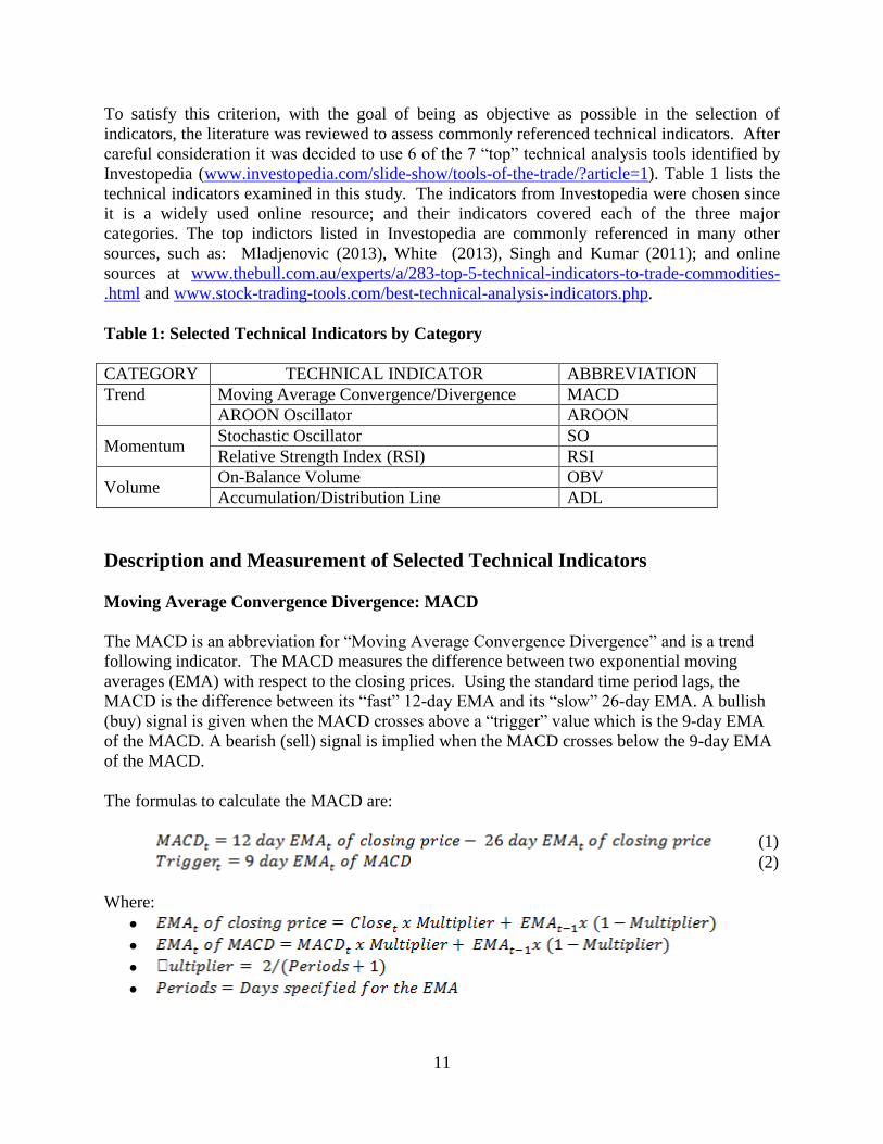
Table 1: Selected Technical Indicators by Category
CATEGORY TECHNICAL INDICATOR ABBREVIATION
Trend Moving Average Convergence/Divergence MACD
AROON Oscillator AROON
Momentum Stochastic Oscillator SO
Relative Strength Index (RSI) RSI
Volume On-Balance Volume OBV
Accumulation/Distribution Line ADL
Description and Measurement of Selected Technical Indicators
Moving Average Convergence Divergence: MACD
The MACD is an abbreviation for “Moving Average Convergence Divergence” and is a trend
following indicator. The MACD measures the difference between two exponential moving
averages (EMA) with respect to the closing prices. Using the standard time period lags, the
MACD is the difference between its “fast” 12-day EMA and its “slow” 26-day EMA. A bullish
(buy) signal is given when the MACD crosses above a “trigger” value which is the 9-day EMA
of the MACD. A bearish (sell) signal is implied when the MACD crosses below the 9-day EMA
of the MACD.
The formulas to calculate the MACD are:
(1)
(2)
Where:

12
Note that to start the calculation of the EMA in the first period (t=1), use a simple moving
average (SMA) as the previous period's EMA.
Aroon – Dawns Early Light
Aroon is a word in Sanskrit that refers to “Dawn’s Early Light” and is a trend indicator that tries
to assess the strength of a trend in the stock price movement. The hypothesis is that a stock is
trending up when a stock is near the top of its price range relative to its previous bottom price; or
trending down if it is closer to the bottom of its price range relative to its previous high price.
To measure this trend, the indicator calculates an Aroon-up; an Aroon-down, and an Aroon-
Oscillator. The formulas using the standard 14-day time period are:
Aroon-Up = 100 x (14 - Days since the 14-day High)/14 (3)
Aroon-Down = 100 x (14 - Days since the 14-day Low)/14 (4)
Aroon Oscillator = Aroon-Up - Aroon-Down (5)
Aroon-Up is 100 if the stock closes at a new high for the given time period. For each day that
passes without another new high, Aroon-Up decreases by an amount equal to (1 / number of
days) x 100. Similarly, an Aroon-Down is 100 if the stock closes at a new low and decreases for
each day after that by an amount equal to (1/number of days)x100.
As an example, if 7 days have passed since the prior High price, and only 2 days have passed
since the prior Low price, then:
Aroon-Up = 100 x (14-7) /14 = 50.00
Aroon-Down = 100 x (14-2) /14 = 85.71
Aroon-Oscillator = 50 – 85.71 = -35.71
An Aroon-Oscillator that crosses below a zero value line is considered a signal of an impending
downtrend; and a cross above a zero value line is considered to be a signal of an impending
uptrend.
Stochastic Oscillator: SO
The stochastic Oscillator is a momentum indicator and focuses on the speed and relative position
of the movements in price; and hypothesizes that momentum changes direction before price. This
indicator measures the current closing price relative to the difference between the high and low
price range over a given period of time.
The formulas for the stochastic oscillator are:
(6)
(7)
13
Where:
C = Current closing price
Lx= Lowest price of the past x trading periods (standard 14 days used)
Hx= Highest price traded during past x trading periods (standard 14 days used)
SMA = simple moving average (standard 3 days used)
The Stochastic Oscillator “K” is above 50 when the closing price, C, is in the upper half of the
range between the high and low price (Hx – Lx); and below 50 when the closing price is in the
bottom half of the range between the high and low price
A bullish signal is when the K value crosses the D in an upward direction. A bearish signal is
when the K crosses below the D value in a downward direction.
Relative Strength Index: RSI
The relative strength index (RSI) is a momentum indicator and is used to signal overbought and
oversold conditions in a security by comparing the magnitude of recent gains in price to recent
losses. The indicator ranges in value between 0 and 100, where 100 is the highest overbought
condition and zero is the highest oversold condition. It is calculated using the following formula:
RSI = 100 – [100 / (1 + RS)] (8)
RS = Average of x-days positive returns / Average of x-days negative returns (9)
In this study, the number of periods (x-days) is set to the standard14 days. A zero RSI means
prices moved lower all 14 periods. In this case the average of x days’ positive returns is set to
zero. An RSI of100 occurs when there are no negative returns. In this case the average of x-days
negative returns is equal to zero and the RS becomes infinitely large, causing RS to be zero and
the RSI to equal 100.
A security is considered overbought (overvalued) once the RSI approaches the 70 level,
suggesting a bearish (sell) signal. Similarly, a security is considered oversold (undervalued) once
the RSI approaches 30, suggesting bullish (buy) signal.
On Balance Volume: OBV
OBV refers to “On Balance Volume” and is a volume indicator. The hypothesis behind the
volume indicator is that volume changes precede price changes. It is hypothesized that it is
likely that before a stock advances, there will be period of increased volume.
OBV measures the buying and selling pressure as a cumulative volume index that increases the
index on days when the stock price increases; and subtracts the index on days when the stock
price decreases. The formula used to calculate OBV is as follows, where the subscript “t”
represents the time:
: (9)
: (10)

14
: (11)
Where:
A rising OBV reflects positive volume pressure that can lead to higher prices. Conversely, falling
OBV reflects negative volume pressure that can foreshadow lower prices. But note that OBV is
argued not to be a stand-alone indicator. It is designed to be used in conjunction with other
indicators, like trend or momentum, to support a buy or sell signal.
Accumulation/Distribution Line: ADL
The Accumulation/Distribution Line (ADL) is a commonly used volume indicator that measures
the “money flow” into or out of a security. To do this, the indicator considers both trading
volume and price together. The intent of the indicator is to determine if traders are
“accumulating” funds or “distributing” funds of a security; so it is a flow of funds measure of
volume.
The ADL indicator is calculated using the following formula:
(12)
(13)
(12) (14)
Where:
MMt = Money Multiplier in period (day) t
MVt = Money Volume in period (day) t
Volumet = trading volume in period (day) t
ADLt = cumulative measure of accumulation distribution in period (day) t
Closet = closing price in period (day) t
Lowt = low price in period (day) t
Hight = high price in period (day) t
Note that the ADL is a cumulative measure and is a running total of each period's money volume
(MV). Interpreting the ADL we observe that the impact of trading volume depends on the price
of the security which determines the money multiplier (MM). The money multiplier (MM)
ranges from +1 to -1. The money multiplier (MM) is +1 when the closing price is equal to the
high price; and MM is equal to -1 when the closing price is equal to the low price. In this case,
trading volume in a period (day) has a greater impact on money flow and the ADL when the
closing price is high.
Note that ADL is argued not to be a stand-alone indicator. It is designed to be used in
conjunction with trend or momentum indicators to support a buy or sell signal. Because of this,
the test of the ADL indicator is done when combined with other indicators.

15
Data and Methodology
Owing to recent and significant advancements in information technology, this study focuses on
the two most recent two years of data, 2013 and 2014; and includes daily data on all firms in the
DOW for each of these years. The portfolio of DOW firms was chosen because it represents an
objective selection of large, well-known securities and should not be affected to any significant
degree by frictions, such as non-synchronous trading that may alter the behavior of investors.
The historical market data for this study is taken from two primary sources: (a) Wharton
Research Data Services (WRDS), which includes the Center for Research in Security Prices
(CRSP); and a commercial database supplied by Kinetick (www.kinetick.com).
Tests of Trading System Performance and Hypothesizes
Several measures of trading performance, commonly examined by both academics and
experienced traders (Davey, 2014; and Chande, 2001), will be used to test the success of the
popular technical indicators identified in this study.
A description of the measures used to identify a successful trading system and the hypothesis
associated with each measure follows.
Percent of Profitable Trades
A common test of success is the percent of profitable trades. According to Davey (2014), the
percentage of profitable trades should exceed 50% to pass a “monkey test”. The money test
assumes stock returns are normally distributed and contends that a random selection of trades
(entry and exit points), like those selected by a monkey, would likely yield profitable returns in
only half the selections. In this respect, a good trading system is considered to be one where the
profitable trades significantly exceed 50% of the total number of trades.
Hypothesis 1: The percent of profitable trades will exceed 50%.
Trading System Rate of Return: HPR and APR
A key measure of a trading system’s success is the rate of return on investment. The rate of
return is measured by the average trade holding period return (HPR) and the average trade
annual percentage return (APR).
The formulas are:
HPR = (Exit Price – Entry Price)/Entry price {over the holding period}
APR = HPR x Holding Periods per year

16
For the trading system to be successful, the average APR of the portfolio is expected to exceed a
buy and hold strategy.
Hypothesis 2: The average trade APR will exceed the percent increase in the market index over
the year.
The HPR and resulting APR of the portfolio is compared to the rate of return of the Dow Jones
Index over the course of the year being studied, not during the same holding period for each
trade, as done in other studies (Fang, Jacobsen, and Qin 2014; Brock, Lakonishok, and LeBaron,
1992; and Sehgal and Garhyan, 2002). A simple example will illustrate the problem associated
with comparing the HPR with the increase in the market index during the same holding period.
Suppose that during the course of a year, the market has four months (e.g. January, April, July,
September) were the growth in the index is very large, say 15% in each of these months; and
four months where the growth is negative 15%; with the remaining months having stable prices
(zero growth). Note that in this example, the market return over the entire year would be zero.
Now assume the trading system signals a buy in each of the four months of growth, and exits
each of these trades at a 10% return. But the trading system did not signal any other buys during
the course of the year, avoiding the periods of market decline. In this case, if the trading system
were compared to the market index during the “holding” periods, the trading system would have
a lower return than the market index (i.e. 10% for the trade versus 15% for the market); and one
might conclude the trade was not successful. Yet in this case the trading system was highly
successful because it invested only during the growth periods, and not during the market
declines; and over the course of the entire year the trading system return would be positive (four
trades with 10% returns) compared to the overall market return which was flat (zero percent
return).
It has also been argued that the using the annualized percent return, APR, is not realistic or
biased because it assumes a trade that only lasts a month, for example, would generate that same
return all year (Sehgal and Garhyan, 2002). The problem with this argument is that it ignores the
opportunity cost of funds. If a trading system performs trades with smaller holding periods, then
the funds are available for other uses for a greater period of time than a portfolio with larger
holding periods. In a sense the APR adjusts for the liquidity value of the trade by adjusting thee
return based on the length of the holding period. In this sense, the APR is considered to be a
valid and important measure of success of the trading system.
Sharpe Ratio (Return Efficiency)
The risk of the portfolio is measured by the Sharpe ratio, sometime referred to as the return
efficiency, which shows the relationship between the risk premium return of the portfolio and its
standard deviation. The Sharpe ratio illustrates the risk to return tradeoff of alternative trading
systems.
Sharpe ratio = (portfolio return – risk free rate) / standard deviation of portfolio return

17
In this study the Sharpe ratio is based on the portfolio’s average percentage return (HPR); and
the risk free rate is measured by the 3-month Treasury bill rate. A portfolio with a higher Sharpe
ratio is considered to have a lower risk.
To assess this dimension, we compare the Sharpe ratio of the trading system portfolio, which in
our study is a portfolio of all Dow stocks, with the Sharpe ratio of the overall Dow Jones market
index (DJI).
Hypothesis 3: The Sharpe ratio of the portfolio (composed of all Dow firms in this study) will
not be significantly lower than the Sharpe ratio of the market index. (Note: a
lower Sharpe represents a higher risk.)
Ratio of Average Winning to Losing Trade Returns
Another measure of success, examined by investors, depends on the average return of the
winning trades compared to the average return of the losing trades. This measure provides
additional insights with respect to the performance of the trading system. A trading system will
be preferred the greater the ratio of average winning to losing returns.
Given the assumption that stock returns are normally distributed, then with a random selection of
trades (i.e. an ineffective trading system), the average returns of winning trades should not differ
statistically from losing trades (using absolute values). So, a signal of a successful trading
system would be if the average returns of the winning trades exceeded the returns (absolute
values) of the losing trades.
To assess this dimension, we test the null hypothesis of equality between the mean return of the
winning trades and the losing trade; where a successful trading system will have a ratio of
winning to losing trade returns that exceeds 1.
Hypothesis 4: The ratio of the absolute value of the average winning to losing trade returns will
exceed 1.0
Maximum Favorable Excursion (MFE) versus Maximum Adverse Excursion (MAE)
The average maximum favorable excursion (MFE) is used by investors to identify a successful
entry signal for a trading system. The MFE measures the maximum amount a security’s price
increases from the entry price while in a trade (i.e. the maximum run-up). A high value for the
MFE implies the entry point is desirable since there is a greater opportunity to capture a
significant gain in price and profits. This information helps gauge how well a trading strategy’s
“entry” conditions predict upcoming price movements.
In the opposite direction to the MFE, the MAE measures the maximum amount the price
decreases (runs down) from the entry point. The average MAE measures how poorly a strategy’s
entry conditions predicts the direction of future price movements. A relatively low percentage
here is desirable since it would imply that the price would not move against the intended
direction of the trade after entering a position.

18
A high MAE works against the MFE, so a successful trading strategy would be one in which the
MFE exceeds the MAE. In this case, the entry signal would select trades where the average run-
up in prices would exceed the average run down in prices.
Hypothesis 5: The average MFE will exceed the average MAE
End of Trade Drawdown (ETD)
The average value of the “End of Trade Drawdown” (ETD) measures the success of the “exit”
strategy of the trading system. The ETD is a measure of the peak price reached in the trade
minus the selling price. It represents the opportunity cost of not selling earlier before the
drawdown occurs. A low value here is best, with a zero ETD representing an ideal exit strategy.
A reasonable goal for the ETD is argued to be a drawdown of 2%. This is based on a common
stop-loss order trading practice where it is suggested that an investor allocate no more than 2% of
available capital on a single trade and is referred to as the “2%-rule”. This restriction is used by
investors that try to stay within acceptable financial limits and controlling risks (see Rockefeller,
2014; tradingpicks.com/stop_loss; and investopedia.com/terms/t/two-percent-rule).
Hypothesis 6: The average ETD is less than 2%.
Results: Performance of Technical Indicators
All the selected indicators listed previously in Table 1 were tested using the standard (typical)
parameters and no optimization (i.e. the changing of parameters to improve results) was
attempted. The results are presented by first looking at the two trend indicators (MACD and
AROON) in Tables 2 and 3; and next the two momentum indicators (SO and RSI) in Tables 4
and 5. The two volume indicators (OBV and ADL) were combined with each of the trend and
momentum indicators because they were not developed to be stand-alone trading models. They
were designed with the assumption that they would be used with other indicators as an additional
selection condition for a buy or sell signal.
MACD with OBV and ADL indicators
In Table 2 the performance results for the MACD as a stand-alone indicator are reported; and
then followed by the MACD combined with the OBV and ADL indicators for the years 2013 and
2014.

19
Table 2: MACD with OBV and ADL
2014 2013
PERFORMANCE
MEASURES MACD
MACD
with
OBV
MACD
with
ADL
MACD
MACD
with
OBV
MACD
with
ADL
Total # of Trades 278 99 119 286 105 123
Percent Profitable Trades 46.76% 61.62% 57.14% 51.40% 71.43% 65.85%
Average Trade HPR 0.715% 2.79% 2.13% 0.99% 4.23% 3.51%
Average Time Trade in
Market (days) 18.56 76.58 54.13 16.15 70.8 45.91
Average Trade APR 14.06% 13.29% 14.36% 22.45% 21.8% 27.93%
Sharpe Ratio 0.457 0.606 0.602 0.683 0.583 0.834
Average Winning Trade
HPR 3.41% 5.67% 5.05% 3.86% 6.84% 6.60%
Average Losing Trade HPR 1.65% 1.85% 1.76% 2.04% 2.30% 2.44%
Ratio Winning/Losing
Trade HPR 2.06 3.07 2.86 1.89 2.97 2.70
Average MFE 3.46% 6.04% 5.20% 4.01% 7.24% 6.29%
Average MAE 1.55% 3.70% 3.21% 1.83% 3.45% 3.04%
Average ETD 2.74% 3.25% 3.07% 3.02% 3.01% 2.78%
The MACD indicator, when used alone generated 278 trades in the year 2014 and 286 trades in
2013 out of the portfolio of 30 Dow firms. When the volume indicators were included, a trade
was only entered or exited when it satisfied both the MACD and volume indicator (either OBV
or ADL) conditions simultaneously. Because of this, the number of trades decreased
significantly to about one-third of the trades when the volume indicators were included. .
A successful trading system is considered to be one where the profitable trades significantly
exceed 50% of the total number of trades. For MACD alone, the percent of profitable trades were
only 46.76% in 2014 and 51.40% in 2013. These values are not significantly different from 50%
and did not pass the “monkey test”. But when the volume indicators OBV and ADL were added
the percent of profitable trades increased above 50%, ranging from 57% to 71%; and the increase
was statistically significant.
The average rate of return of the portfolio is another important measure of overall success. For
the MACD indicator, operating alone in the year 2014, the average holding period return (HPR)
is 0.715%; and with a holding period of only 18.56 days realized an annual percent return (APR)
of 14.06%. This exceeded the annual return of the market index (DJI) of 8.4% for the year 2014.
In the year 2013 the MACD APR is 22.45% but this is not significantly different than the DJI
APR of 23.6% for this year. When the volume indicators were added to the MACD, the average
trade returns (APR) remained at about the same levels and were not significantly different.
20
The risk of the trading portfolios, based on the Sharpe ratios, significantly decreased when the
volume indicators were added to the trading system, except for the MACD with OBV in 2013.
Yet, the Sharpe ratios were all significantly lower than the DJI Sharpe ratios during this time
period of 1.28.
Comparing the average winning trade return to the losing trade return, the ratio is greater than
2.0 in all cases except for the MACD when used alone in 2013. When the volume indicators,
OBV and ADL, were added to the trading system, the ratio of the average winning returns to the
losing returns increased from about 2 to 3. The increase in the ratio was statistically significant,
supporting the hypothesis that the volume indicators added value to the success of the trading
system, based on this dimension.
The success of the trading system entry condition in predicting upcoming price movements is
gauged by examining both the average maximum favorable excursion (MFE) and the maximum
Adverse Excursion (MAE). The MFE was positive and statistically significant in both years for
all measures, and were greater than the MAE values. The MAE values for the MACD alone
were between 1.55% and 1.83%, while the MFE were all higher at 3.46% and 4.01%. When the
volume indicators were added, both the MFE and MAE increased, but the MFE values increased
more than the MAE, and the difference was statistically significant.
The average “End of Trade Drawdown” (ETD) measures the success of the “exit” strategy of the
trading system. A low value here, less than 2%, is desired. Table 2 shows the average ETD
levels were around 3% and were statistically significant. Adding the volume indicators did not
improve (i.e. lower) the ETD values. The difference between the EDT values with and without
the volume measures were not statistically significant. The data indicates that an ideal “exit”
signal could yield an increase in the average return of the trading system by as much as 3%.
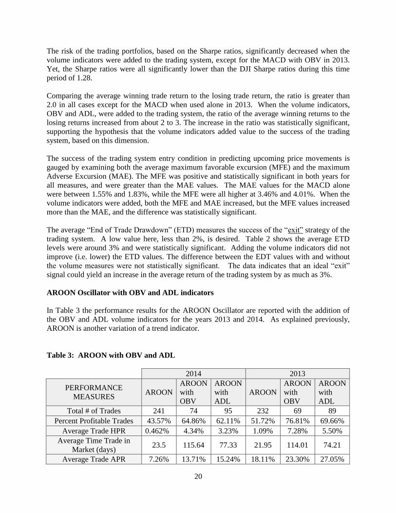
AROON Oscillator with OBV and ADL indicators
In Table 3 the performance results for the AROON Oscillator are reported with the addition of
the OBV and ADL volume indicators for the years 2013 and 2014. As explained previously,
AROON is another variation of a trend indicator.
Table 3: AROON with OBV and ADL
2014 2013
PERFORMANCE
MEASURES AROON
AROON
with
OBV
AROON
with
ADL
AROON
AROON
with
OBV
AROON
with
ADL
Total # of Trades 241 74 95 232 69 89
Percent Profitable Trades 43.57% 64.86% 62.11% 51.72% 76.81% 69.66%
Average Trade HPR 0.462% 4.34% 3.23% 1.09% 7.28% 5.50%
Average Time Trade in
Market (days) 23.5 115.64 77.33 21.95 114.01 74.21
Average Trade APR 7.26% 13.71% 15.24% 18.11% 23.30% 27.05%

21
Sharpe Ratio 0.290 0.452 0.407 1.093 0.792 0.592
Average Winning Trade
HPR 3.50% 8.39% 6.96% 4.51% 10.15% 9.34%
Average Losing Trade HPR 1.88% 3.13% 2.89% 2.57% 2.25% 3.31%
Ratio Winning/Losing
Trade HPR 1.86 2.68 2.41 1.75 4.52 2.82
Average MFE 3.79% 8.67% 7.03% 4.67% 10.62% 8.87%
Average MAE 1.88% 4.71% 3.76% 2.23% 4.52% 3.71%
Average ETD 3.33% 4.33% 3.80% 3.58% 3.34% 3.37%
The AROON indicator, when used alone, generated 241 trades in the year 2014; and 232 trades
in 2013. When the volume indicators were included the number of trades decreased, as expected,
to about one-third of its original level.
The percent of profitable trades for the AROON Oscillator, when used as a stand-alone indicator,
was only 43.57% in 2014 and 51.72% in 2013. These values are not significantly different from
50% and did not pass the “monkey test”. But when the volume indicators OBV and ADL were
added the percent of profitable trades increased above 50%, ranging from 62.11% to 76.81%;
and the increase was statistically significant.
The average holding period return (HPR) for the AROON operating alone in the year 2014 is
0.462%; and with a holding period of 23.5 days realized an annual percent return (APR) of only
7.26%. This was lower than the annual return of the market index (DJI) of 8.4% for the year
2014. In the year 2013 the AROON APR of 18.11% is also lower than the DJI APR of 23.6%.
When the volume indicators were added to the AROON Oscillator, the average trade APR values
all increased significantly, ranging between 13.71% and 15.24% in 2014; and between 23.3%
and 27.05% in 2013. The APR values exceeded the DJI returns in 2014; but in 2013, only the
AROON with ADL annual return of 27.05% exceeded the DJI return.
The Sharpe ratios of the trading system are all lower than the DJI Sharpe ratio of 1.28 in both
years. In 2014, the volume indicators did significantly lower the risk (i.e. higher Sharpe ratios),
but this was not the case in 2013 and the Sharpe ratios declined.
Comparing the average winning trade return to the losing trade return, the ratio is close to or
greater than 2.0 in all cases. When the volume indicators, OBV and ADL, were added to the
trading system, the ratio of the average winning returns to the losing returns increased to higher
values, ranging from 2.41 to 4.52. The increases in the ratios were statistically significant and the
volume indicators added value to the success of the trading system.
Referring to the maximum favorable excursion (MFE), the entry strategy was much more
successful when the volume indicators were included. In 2014, the MFE increased from 3.79%
to 8.67% when OBV was added; and to 7.03% with ADL. In 2013, the MFE increased from
4.67% to 10.62% with OBV; and to 8.87% with ADL.

22
An entry strategy is successful if the MAE is relatively low. In this respect, the MAE values
were all significantly lower than the MFE values in all cases, implying that the entry signals
identified points where the average run-up in prices exceeded the average run down in prices.
When the volume indicators were added, the MAE values increased significantly but remained
below the MFE values.
The average “End of Trade Drawdown” (ETD) values were around 3.5% and were significantly
greater than 2%. Adding the volume indicators did not improve (i.e. lower) the ETD values; and
in the year 2014 ETD increased significantly to 4.33%; but in the other cases there was no
significant difference. The data indicates that an ideal “exit” signal could yield an increase in the
average return of the trading system about 3.5%.
Stochastic Oscillator (SO) with OBV and ADL indicators
In Table 4 the results for the Stochastic Oscillator (SO) are reported along with the OBV and
ADL volume indicators for the years 2013 and 2014. As indicated previously, the Stochastic
Oscillator is a momentum indicator.
Table 4: Stochastic Oscillator with OBV and ADL
2014 2013
PERFORMANCE
MEASURES SO
SO
with
OBV
SO
with
ADL
SO
SO
with
OBV
SO
with
ADL
Total # of Trades 564 254 273 567 269 281
Percent Profitable Trades 49.29% 58.27% 53.48% 46.38% 57.99% 52.31%
Average Trade HPR 0.610% 0.726% 0.512% 0.554% 0.837% 0.803%
Average Time Trade in
Market (days) 9.04 18.55 16.77 8.68 18.45 15.09
Average Trade APR 24.63% 14.28% 11.15% 23.29% 16.55% 19.43%
Sharpe Ratio 1.255 0.574 0.355 1.066 0.617 0.637
Average Winning Trade
HPR 2.76% 2.56% 2.50% 2.97% 2.99% 3.08%
Average Losing Trade HPR 1.48% 1.84% 1.77% 1.54% 2.14% 1.70%
Ratio Winning/Losing
Trade HPR 1.87 1.39 1.41 1.93 1.40 1.81
Average MFE 2.50% 2.68% 2.38% 2.62% 3.11% 2.84%
Average MAE 1.32% 2.28% 2.35% 1.50% 2.40% 2.14%
Average ETD 1.89% 1.96% 1.87% 2.07% 2.27% 2.04%
The SO when used alone, generated many more trades compared to the other indicators. In the
year 2014 there were 564 trades; and in 2013 there were 567 trades. When the volume indicators
were included the number of trades was cut approximately in half.

23
The percent of profitable trades for the SO, when used alone, was only 49.29% in 2014 and
46.38% in 2013. These values are not significantly different from 50% and did not pass the
“monkey test”. But when the volume indicator OBV was added, the percentage of profitable
trades increased to 58.27% in 2014 and to 57.99% in 2013; and was statistically significant,
passing the monkey test. The ADL indicator, although increasing the percentage of profitable
trades by a few percentage points above the 50% did not pass the monkey test.
The average holding period return (HPR) for the Stochastic Oscillator (SO) operating alone in
the year 2014 is 0.61%; and with a holding period of 9.04 days realized an annual percent return
(APR) of 24.63%. This was significantly greater than the annual return of the market index (DJI)
of 8.4% for the year 2014. In the year 2013 the SO APR of 23.29% is on par with the DJI APR
of 23.6%. When the volume indicators were added to the SO, the average trade APR values all
decreased significantly, ranging between 14.28% and 11.15% in 2014; and between 16.55% and
19.43% in 2013.
The Sharpe ratio of the trading system was significantly below the DJI Sharpe ratio of 1.28
except for the year 2014 when the SO was used alone without the volume indicators. In this year
the SO indicator had a Sharpe ratio of 1.255 which was on par with the DJI. Also, adding the
volume indicators significantly increased the risk of this trading system.
Comparing the average winning trade return to the losing trade return, the ratio is less than 2.0 in
all cases; whereas with the MACD and AROON indicators these ratios were greater than 2.
When the volume indicators, OBV and ADL, were added to the trading system, the ratio of the
average winning returns to the losing returns did not improve, and declined in value. With
respect to this dimension, the performance of the trading system declined when the volume
indicators were included.
Comparing the maximum favorable excursion with the maximum adverse excursion, the average
MFE values all exceeded the average MAE values, and in this sense were successful. But when
adding the volume indicators, the performance of the system declined. In this case, the MAE
values significantly increased in both years, while the MFE values remained at about the same
levels (no significant difference). With the inclusion of the volume indicators, the MFE values
were not significantly higher than the MAE, except for the SO with OBV in 2013.
The average ETD measures the success of the “exit” strategy and represents the opportunity cost
of not selling earlier before a drawdown occurs. A low value here is best. Table 3 shows the
average ETD levels were at or near 2%, and were significantly lower than the ETD values for the
MACD and AROON indicators.
The average “End of Trade Drawdown” (ETD) values were at acceptable levels, below or near
2%; and were much lower than the prior trading systems (MACD and AROON). Adding the
volume indicators did not change the ETD values. The ETD was clearly superior with the SO
indicator compared to the MACD and AROON indicators.

24
Relative Strength Index (RSI) with OBV and ADL indicators
In Table 5 the results of the Relative Strength Index (RSI) are reported with the OBV and ADL
volume indicators for the years 2013 and 2014. As indicated previously, the Relative Strength
Index is a momentum indicator.
Table 5 Relative Strength Index with OBV and ADL
2014 2013
PERFORMANCE
MEASURES RSI
RSI
with
OBV
RSI
with
ADL
RSI
RSI
with
OBV
RSI
with
ADL
Total # of Trades 102 6 31 91 8 22
Percent Profitable Trades 83.33% 100.00% 80.65% 86.81% 87.50% 86.36%
Average Trade HPR 3.12% 5.14% 2.91% 3.71% 3.73% 3.72%
Average Time Trade in
Market (days) 34.75 24.83 41.29 33.56 26.25 37.95
Average Trade APR 32.78% 75.49% 25.72% 40.36% 51.91% 35.76
Sharpe Ratio 1.30 2.015 0.899 1.207 1.025 1.157
Average Winning Trade
HPR 4.47% 5.14% 4.42% 4.53% 4.54% 4.66%
Average Losing Trade HPR 3.60% 0.00% 3.38% 1.68% 1.884% 2.22%
Ratio Winning/Losing
Trade HPR 1.24 na 1.31 2.70 2.41 2.09
Average MFE 4.50% 5.16% 4.32% 4.74% 4.86% 4.50%
Average MAE 4.12% 3.58% 4.02% 2.98% 2.90% 3.36%
Average ETD 1.38% 0.03% 1.41% 1.02% 1.13% 0.79%
The RSI criteria, when used alone without volume conditions, did not generate as many trades
compared to the other indicators. In the year 2014 there were only 102 trades; and in 2013 only
91 trades. When the volume indicators were included the number of trades became very small,
ranging between 6 and 31 trades. This limits the statistical inferences one can make with respect
to the impact of adding the volume indicators.
The percent of profitable trades for the RSI, when used alone, was 83.33% in 2014 and 86.81%
in 2013. These values are significantly higher than the other technical indicators (MACD,
AROON, and SO) and are above 50%; clearly passing the “monkey test”. When the volume
indicators OBV and RSI were added, the percentage of profitable trades remained at
approximately the same high level; except for the exceptionally high 100% profit rate realized in
2014 for the OBV indicator. However, the number of trades (only 6) is too small to draw
statistical inferences.
The average holding period return (HPR) for the RSI operating alone in the year 2014 is 3.12%;
and with a holding period of 34.75 days realized an annual percent return (APR) of 32.78%. This

25
was significantly greater than the annual return of the market index (DJI) of 8.4% for the year
2014. In the year 2013 the RSI APR is 40.35% and also exceeds the DJI APR of 23.6%. When
the OBV volume indicators is added to the RSI, the average trade APR values increased
significantly to 75.49% in 2014 and to 51.96% in 2013. But adding the ADL volume indicator
lowered the APR values, but they were equivalent to the market DJI return in 2014; and higher
than the market in 2013. With respect to the APR, the RSI outperformed the other indicators
(MACD, AROON, and SO).
The Sharpe ratio of the RSI was also superior to the other indicators. The Sharpe ratios for the
RSI operating alone are on par with the DJI index Sharpe ratio of 1.28. When adding the OBV
volume indicator the Sharpe ratio increased substantially to 2.015 in 2014; but dropped
somewhat in 2013 to 1.025. Adding the ADL indicator, lowered the Sharpe value significantly
in 2014 but only marginally in 2013. Yet in all cases, the RSI risk levels were lower than the
other indicators.
Comparing the average winning trade return to the losing trade return, the ratios exceeded 1.0 in
2014; and were much higher in 2014, exceeding 2.0 in all cases. The addition of the volume
indicators did not change the ratios (no statistically significant differences) from the RSI used by
itself. This finding does not support the hypothesis that the volume indicators improved trading
system with respect to this dimension.
A relatively high average value of the maximum favorable excursion (MFE) compared to the
maximum adverse excursion (MAE) is used to identify a successful entry strategy for a trading
system. In Table 4 the average MFE values all exceeded the average MAE values; supporting
the hypothesis that the entry criteria were successful. But adding the volume indicators did not
improve the entry performance as there was not a significant difference in the relative values of
MFE and MAE.
Comparing the maximum favorable excursion with the maximum adverse excursion, the average
MFE values all exceeded the average MAE values. For the RSI operating alone, the difference
was not statistically significant in 2014, but was significant in 2013. When adding the volume
indicators, MFE was significantly greater than the MAE except for the ADL in 2014.
With respect to the “exit” strategy of the trading system, Table 5 shows the average ETD levels
were near 1%, and significantly less than the desired target of 2%. This supports the hypothesis
that the exit condition was successful, and the securities were sold before a significant drawdown
occurred.
Summary of Findings: Overall Performance of Trading Rules
In the section we summarize the performance of the trading rules. Table 6 summarizes the tests
of the success of the technical indicators without the inclusion of the volume indicators.

26
Table 6: Test of success of Trading Rules excluding volume indicators
TEST OF
DESIREABLE
PERFORMANCE
Year 2014 Year 2013
MACD AROON SO RSI MACD AROON SO RSI
Profitable trades > 50% no no no yes**
yes yes no yes**
Average APR > Market
Return
Yes* no yes
** yes
** no no no yes
**
Sharpe Ratio >= Market
Sharpe
no no yes yes no no no yes
Winning/Losing trade
returns> 1.0
yes**
Yes**
yes**
yes**
yes**
yes**
yes**
yes**
Average MFE > MAE yes**
yes**
yes**
yes yes**
yes**
yes**
yes**
Average ETD < 2% yes yes yes yes no no no yes**
* Statistically significant at 10% or greater;
**statistically significant at 5% or greater
The test results show limited success with respect to profitability. The percent of profitable
trades were below 50% in three of the four indicators in 2014; and in the year 2013 the average
percent returns (APR) were below the market returns in three of the four indicators. However, it
is noteworthy that the RSI indicator was profitable in both years with lower risk than the overall
market.
Focusing on the viability of the entry signal for the trades, there was significant success. Both
the ratio of the average winning/losing trade returns exceeded 1 and the average MFE exceeded
MAE for all indicators in both years. However, there were lost opportunities with respect to the
exit signals in the year 2013 with ETD levels greater than 2% three of the four indicators.
When the volume indicators are included the overall results improved with respect to
profitability but not with the exit conditions. Table 7 shows that with the addition of the OBV
indicator, the percent of profitable trades were greater than 50% in all cases; and the average
percent returns (APR) exceeded the market returns for all indicators in 2014; but there was no
improvement for the year 2013 with either APR or ETD.
Table 7: Test of success of Trading Rules including On-Balance Volume (OBV)
INDICATORS
WITH OBV
Year 2014 Achievements Year 2013 Achievements
DESIREABLE
PERFORMANCE
MACD
+OBV
AROON
+OBV
SO
+OBV
RSI
+OBV
MACD
+OBV
AROON
+OBV
SO
+OBV
RSI
+OBV
Profitable trades >
50%
yes**
yes**
yes* yes
** yes
** yes
** yes
* yes
**
Average APR >
Market Return
yes yes**
yes* yes
** no no no yes
**
Sharpe Ratio >=
Market Sharpe
no no no yes* no no no yes

27
Winning/Losing
trade returns> 1.0
yes**
Yes**
yes**
yes**
yes**
yes**
yes**
yes**
Average MFE >
MAE
yes**
yes**
no yes**
yes**
yes**
yes* yes
**
Average ETD <
2%
no yes**
yes yes* no no no yes
**
* Statistically significant at 10% or greater;
**statistically significant at 5% or greater
When the Accumulation/Distribution Line is included with each of the basic indicators instead of
the OBV indicator, the profit ratings improved. Table 8 shows the APR exceeded the market
returns in all cases except for AROON+ADL and SO+ADL in 2013. The RSI was again the best
trading rule of the group with successful performance measures in all categories in 2013 and in 5
of the 6 categories in 2014.
Table 8: Test of success of Trading Rules including Accumulation/Distribution Line (ADL)
INDICATORS
WITH ADL
Year 2014 Achievements Year 2013 Achievements
DESIREABLE
PERFORMANCE
MACD
+ADL
AROON
+ADL
SO
+ADL
RSI
+ADL
MACD
+ADL
AROON
+ADL
SO
+ADL
RSI
+ADL
Profitable trades >
50%
yes* yes
* yes yes
** yes yes
** yes yes
**
Average APR >
Market Growth
yes**
yes**
yes**
yes**
yes no no yes**
Sharpe Ratio >=
Market Sharpe
no no no no no no no yes
Winning/Losing
trade returns> 1.0
yes**
yes**
yes**
yes yes**
yes**
yes Yes**
Average MFE >
MAE
yes**
yes**
yes yes yes**
yes**
yes yes
Average ETD < 2% no no yes yes**
no no no yes**
* Statistically significant at 10% or greater;
**statistically significant at 5% or greater
Conclusion
Considering a multi-dimensional objective function, some encouraging results were discovered
with respect to the viability of technical analysis and algorithmic trading. Performance was
measured not only by the overall return efficiency, but by the success of the trading rule entry
and exit signals.
With respect to return efficiency, three of the four indicators, when used independently, without
volume conditions did not do well. But, the returns improved significantly once the volume
indicators were included. Trading volume has clearly added to the predictability of the trading
rules with the APR exceeding the market returns in 6 of the 8 cases once the ADL volume
indicator was included.
28
The entry conditions of the trading rules were also quite successful. In all cases the maximum
favorable excursions exceeded the maximum adverse excursions. But the exit conditions only
had limited success. The bright spot was the RSI indicator which had ETD values consistently
less than 2%. More attention to developing exit conditions could yield significant
improvements.
The trading rules were also more successful in 2014 than in 2013. One possible explanation is
the differences in the market volatility during these two years. In 2013, there was a persistent
bull market with very little volatility compared to other years. Sturm (2013) explains that since
technical analysis measures beliefs, it follows that the most value from technical analysis would
come from markets with the greatest difference in beliefs. As beliefs differ, price volatility is
expected to increase, so the success of technical analysis should be positively related to
volatility. Because of this, technically analysis is less likely to be helpful in markets with low
volatility as was the case in this study in the year 2013.
To support the findings in this study, future research is encouraged selecting different markets
with different degrees of volatility.
References
Boehner, R., & Gold, S. (2013). Herding Behavior in the DJIA 2005-2009. Journal of Applied Financial
Research, Volume II, 51-67.
Boehner, R., & Gold, S. (2014). An Evaluation of the Causes, Extent, and Initiators of Herding Behavior.
Journal of Applied Financial Research, Volume II, 118-136.
Brock, W., Lakonishok, J., & LeBaron, B. (1992). Simple technical trading rules and the stochastic
properties of stock returns. Journal of Finance, 47(5), 1731–1764.
Chande, Tushar S. (2001). Beyond Technical Analysis: How to Develop and Implement a Winning
Trading System (2nd
ed.). Hoboken, NJ: John Wiley & Sons.
Davey, K. J. (2014). Building Winning Algorithmic Trading Systems: A Trader’s Journedy from Data
Mining to Monte Carlo Simulation to Live Trading. Hoboken, NJ: John Wiley & Sons.
Fang, J., Jacobsen, B., & Qin, Y. (2014). Predictability of the simple technical trading rules: An out-of-
sample test. Review of Financial Economics, 23, 30–45.
Ferson,W. E., Sarkissian, S., & Simin, T. T. (2003). Spurious regressions in financial economics?,
Journal of Finance, 58(4), 1393–1414.
Jumah A., Bashar F., & Muneer A. (2014). Advantages of Using Technical Analysis to Predict Future
Prices on the Amman Stock Exchange. International Journal of Business and Management, 9(2), 1-
16.
Kirilenko, A. A., & Lo, A. W. (2013). Moore’s Law versus Murphy’s Law: Algorithmic Trading and Its
Discontents. Journal of Economic Perspectives, 27(2), 51–72.

29
Lo, A. W., & MacKinlay, A. C. (1990). Data-snooping biases in tests of financial asset pricing models.
Review of Financial Studies, 3(3), 431–468.
Marshall, B. R. (2007). Does Intraday Technical Analysis in the U.S. Equity Market Have Value? Massey
University.
Mladjenovic, P. (2013). Stock Investing For Dummies (2nd
Ed.). Hoboken, NJ: John Wiley & Sons.
Rockefeller, Barbara (2014). Technical Analysis for Dummies (3rd
Ed.). Hoboken, NJ: John Wiley &
Sons.
Sehgal, S., Garhyan, A. (2002). Abnormal returns using technical analysis: The Indian experience.
Finance India, 16(1), 181-203.
Singh, R. & Kumar, A. (2011). Intelligent Stock Trading Technique using Technical Analysis.
International Journal of Management & Business Studies, 1(1), 47-49.
Sturm, R. R. (2013). Market Efficiency and Technical Analysis Can they Coexist?. Research in Applied
Economics, 5(3), 1-14.
Tepper, T. (2015). Can You Really Beat the Market?. Money.com, Available at
http://time.com/money/3717466/can-you-really-beat-the-market/
Treleaven, P., Galas, M., & Hand, V. L. (2013). Algorithmic Trading Review. Communications of the
acm, (56(11), 76-85.
White, R. (2013). Technical Analysis Indicator That Works Turns Positive For These Stock. Forbes.com,
Available at www.forbes.com/sites/greatspeculations/2013/04/15/technical-analysis-indicator-that-
works-turns-positive-for-these-stocks/
About the Author
Steven Gold is a professor in the Saunders College of Business at the Rochester Institute of
Technology in the Finance and Accounting department. He has a PhD in economics from the
State University of New York at Binghamton. His current research interests are in financial
markets and behavioral economics. He is a past president of the Association of Business
Simulations and Experiential Learning, and has published several simulations. His most recent
business simulation is “Beat the Market”, published with Gold Simulations. Contact: Saunders
College of Business, Rochester Institute of Technology, 106 Lomb Memorial Dr., Rochester,
New York 14623-5608; +1 585-475-2318; [email protected].

Copyright of Journal of Applied Financial Research is the property of Academy of BusinessResearch and its content may not be copied or emailed to multiple sites or posted to a listservwithout the copyright holder's express written permission. However, users may print,download, or email articles for individual use.