Embed Size (px)
Citation preview
Department of Mathematics and Statistics
The Well-posedness and Solutions of
Boussinesq-type Equations
Qun Lin
This thesis is presented for the Degree of
Doctor of Philosophy of
Curtin University of Technology
March 2009
Declaration
To the best of my knowledge and belief, this thesis contains no material pre-
viously published by any other person except where due acknowledgment has been
made.
This thesis contains no material which has been accepted forthe award of any
other degree or diploma in any university.
Signature:
Date: 13 March 2009
i
Acknowledgments
I am extremely grateful to my supervisor, Professor Yong Hong Wu, for his
guidance and support during my study. I also thank my co-supervisor, Professor
Shaoyong Lai, for his encouragement and Professor Kok Lay Teo for his helpful
advice. Finally, I sincerely thank all the students and staff in the Department of
Mathematics and Statistics for their encouragement duringmy study at Curtin.
ii
Abstract
We develop well-posedness theory and analytical and numerical solution
techniques for Boussinesq-type equations. Firstly, we consider the Cauchy prob-
lem for a generalized Boussinesq equation. We show that under suitable conditions,
a global solution for this problem exists. In addition, we derive sufficient conditions
for solution blow-up in finite time.
Secondly, a generalized Jacobi/exponential expansion method for finding ex-
act solutions of non-linear partial differential equations is discussed. We use the
proposed expansion method to construct many new, previously undiscovered exact
solutions for the Boussinesq and modified Korteweg-de Vriesequations. We also
apply it to the shallow water long wave approximate equations. New solutions are
deduced for this system of partial differential equations.
Finally, we develop and validate a numerical procedure for solving a class of
initial boundary value problems for the improved Boussinesq equation. The finite
element method with linear B-spline basis functions is usedto discretize the equa-
tion in space and derive a second order system involving onlyordinary derivatives.
It is shown that the coefficient matrix for the second order term in this system is
invertible. Consequently, for the first time, the initial boundary value problem can
be reduced to an explicit initial value problem, which can besolved using many
accurate numerical methods. Various examples are presented to validate this tech-
nique and demonstrate its capacity to simulate wave splitting, wave interaction and
blow-up behavior.
iii
List of Publications Related to ThisThesis
1. Qun Lin, Yong Hong Wu, Ryan Loxton and Shaoyong Lai, LinearB-spline
finite element method for the improved Boussinesq equation,Journal of Com-
putational and Applied Mathematics, 224 (2009) 658-667.
2. Qun Lin, Yong Hong Wu and Ryan Loxton, On the Cauchy problemfor a
generalized Boussinesq equation, Journal of MathematicalAnalysis and Ap-
plications, 353 (2009) 186-195.
3. Qun Lin, Yong Hong Wu and Ryan Loxton, A generalized expansion method
for non-linear wave equations, Journal of Physics A: Mathematical and The-
oretical, accepted for publication.
4. Qun Lin, Yong Hong Wu and Shaoyong Lai, On global solution of an initial
boundary value problem for a class of damped nonlinear equations, Nonlinear
Analysis: Theory, Methods and Applications, 69 (2008) 4340-4351.
iv
Contents
Declaration i
Acknowledgments ii
Abstract iii
List of Publications Related to This Thesis iv
List of Figures viii
List of Tables ix
1 Introduction 1
1.1 Background . . . . . . . . . . . . . . . . . . . . . . . . . . . . . . 1
1.2 Objectives . . . . . . . . . . . . . . . . . . . . . . . . . . . . . . . 5
1.3 Outline of the thesis . . . . . . . . . . . . . . . . . . . . . . . . . . 7
2 Review 8
2.1 An overview . . . . . . . . . . . . . . . . . . . . . . . . . . . . . . 8
2.2 Well-posedness theory . . . . . . . . . . . . . . . . . . . . . . . . 8
2.3 Exact solutions . . . . . . . . . . . . . . . . . . . . . . . . . . . . 12
2.4 Numerical methods . . . . . . . . . . . . . . . . . . . . . . . . . . 17
3 On the Cauchy problem for a generalized Boussinesq equation 23
3.1 Introductory remarks . . . . . . . . . . . . . . . . . . . . . . . . . 23
v

3.2 Preliminary results . . . . . . . . . . . . . . . . . . . . . . . . . . 24
3.3 Main results . . . . . . . . . . . . . . . . . . . . . . . . . . . . . . 32
3.4 Concluding remarks . . . . . . . . . . . . . . . . . . . . . . . . . . 38
4 A generalized expansion method for non-linear wave equations 39
4.1 Introductory remarks . . . . . . . . . . . . . . . . . . . . . . . . . 39
4.2 Preliminary results . . . . . . . . . . . . . . . . . . . . . . . . . . 40
4.3 A generalized expansion method . . . . . . . . . . . . . . . . . . . 46
4.4 Traveling wave solutions for the Boussinesq equation . .. . . . . . 50
4.5 Traveling wave solutions for the modified KdV equation . .. . . . 60
4.6 Traveling wave solutions for the shallow water long waveapproxi-
mate equations . . . . . . . . . . . . . . . . . . . . . . . . . . . . 66
4.7 Concluding remarks . . . . . . . . . . . . . . . . . . . . . . . . . . 68
5 Linear B-spline finite element method for the improved Boussinesq equa-
tion 70
5.1 Introductory remarks . . . . . . . . . . . . . . . . . . . . . . . . . 70
5.2 Problem statement . . . . . . . . . . . . . . . . . . . . . . . . . . 72
5.3 Numerical method . . . . . . . . . . . . . . . . . . . . . . . . . . 72
5.4 Numerical examples . . . . . . . . . . . . . . . . . . . . . . . . . 75
5.5 Concluding remarks . . . . . . . . . . . . . . . . . . . . . . . . . . 85
6 Summary and further research 86
6.1 Summary . . . . . . . . . . . . . . . . . . . . . . . . . . . . . . . 86
6.2 Further research . . . . . . . . . . . . . . . . . . . . . . . . . . . . 88
Bibiography 89
vi
List of Figures
4.1 The plot of the solutionu4 to the Boussinesq equation (4.13) with
α1 = −1, α2 = −1, α3 = −3, m = 0.99, k = 1 andν = −1 and
the initial status ofu4. . . . . . . . . . . . . . . . . . . . . . . . . . 55
4.2 The plot of the solutionu7 to the Boussinesq equation (4.13) with
α1 = −1, α2 = −1, α3 = −3,m = 0.9, k = 1 andν = −2 and the
initial status ofu7. . . . . . . . . . . . . . . . . . . . . . . . . . . . 56
4.3 The plot of the solutionu6 to the modified KdV equation (4.31)
with m = 0.95, k = 1 andγ = 0.96 and the initial status ofu6. . . . 65
4.4 The plot of the solutionu6 to the modified KdV equation (4.31)
with m = 0.95, k = 1 andγ = −0.96 and the initial status ofu6. . . 66
4.5 The plot of the solutionu1 of the shallow water long wave approxi-
mate equations (4.37) withm = 0.99, ν = −2 andϑ = γ = 1 and
the initial status ofu1. . . . . . . . . . . . . . . . . . . . . . . . . . 68
4.6 The plot of the solutionv1 to the shallow water long wave approxi-
mate equations (4.37) withm = 0.99, ν = −2 andϑ = γ = 1 and
the initial status ofv1. . . . . . . . . . . . . . . . . . . . . . . . . . 69
5.1 Relationship betweenh andE for Example 5.1. . . . . . . . . . . . 77
5.2 Numerical errors versus time atx = 10 andx = 50 for Example 5.1. 78
5.3 Single soliton solution for Example 5.1. . . . . . . . . . . . . .. . 79
5.4 Wave break-up solution for Example 5.2. . . . . . . . . . . . . . .80
vii
5.5 Inelastic collision withη1 = 1.0 andη2 = 0.5 in Example 5.3. The
contour line on the right illustration starts from 0.01 and the level
step is 0.2. . . . . . . . . . . . . . . . . . . . . . . . . . . . . . . . 82
5.6 Inelastic collision withη1 = 0.5 andη2 = 2.0 in Example 5.3. The
contour line on the right illustration starts from 0.01 and the level
step is 0.3. . . . . . . . . . . . . . . . . . . . . . . . . . . . . . . . 82
5.7 Elastic collision withη1 = 0.4 andη2 = 0.4 in Example 5.3. The
contour line starts from 0.01 and the level step is 0.1. . . . . .. . . 83
5.8 Inelastic collision withη1 = 1.0 andη2 = 1.0 in Example 5.3. The
contour line starts from 0.01 and the level step is 0.2. . . . . .. . . 83
5.9 Elastic collision withη1 = 0.5 andη2 = 0.5 in Example 5.3. The
contour line starts from 0.01 and the level step is 0.1. . . . . .. . . 84
5.10 Solution blow-up in Example 5.4. . . . . . . . . . . . . . . . . . . 85
viii
List of Tables
4.1 Definition of the constantspj,l(γ), j = 1, . . . , 12, l = 0, . . . , 4. . . . 41
5.1 Comparison of the numerical results and exact solution for Example
5.1. . . . . . . . . . . . . . . . . . . . . . . . . . . . . . . . . . . 77
5.2 Numerical results for Example 5.4. . . . . . . . . . . . . . . . . . .85
ix
Chapter 1
Introduction
1.1 Background
The propagation of surface waves is of fundamental and practical importance in
oceanography and marine engineering. Boussinesq-type equations are capable of
providing accurate description of water evolution in coastal regions (see [27, 87]).
The earliest original Boussinesq equation was derived by Boussinesq in 1870s which
takes into account the effects of weak dispersion due to finite depth and weak non-
linearity due to finite amplitude. Boussinesq-type equations also can be applied
to many other areas of mathematical physics dealing with wave phenomena. Ap-
plications to waves in one-dimensional anharmonic lattices, ion acoustic waves in
plasmas, and acoustical waves on circular elastic rods are described in references
[41, 90, 91]. In addition, according to [38] (as quoted by Makhankov [73]), Boussi-
nesq equation is also closely connected with the so-called Fermi-Pasta-Ulam prob-
lem.
The general form of the1 + 1 dimensional Boussinesq equation is
utt + α1uxx + α2uxxxx + α3
(u2)xx
= 0, (1.1)
whereu := u(x, t) represents the wave height from the free surface in the case of
shallow water wave propagation,αj , j = 1, 2, 3, are known constants, and the sub-
scripts denote partial differentiation. In the literature, the Boussinesq equation (1.1)
with αj = −1 (j = 1, 2, 3) is typically referred to as the “bad” or ill-posed Boussi-
1
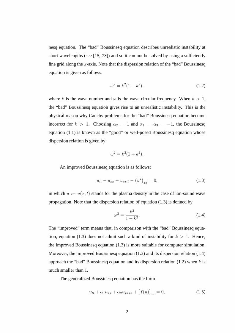
nesq equation. The “bad” Boussinesq equation describes unrealistic instability at
short wavelengths (see [15, 73]) and so it can not be solved byusing a sufficiently
fine grid along thex-axis. Note that the dispersion relation of the “bad” Boussinesq
equation is given as follows:
ω2 = k2(1 − k2), (1.2)
wherek is the wave number andω is the wave circular frequency. Whenk > 1,
the “bad” Boussinesq equation gives rise to an unrealistic instability. This is the
physical reason why Cauchy problems for the “bad” Boussinesq equation become
incorrect fork > 1. Choosingα2 = 1 andα1 = α3 = −1, the Boussinesq
equation (1.1) is known as the “good” or well-posed Boussinesq equation whose
dispersion relation is given by
ω2 = k2(1 + k2).
An improved Boussinesq equation is as follows:
utt − uxx − uxxtt −(u2)xx
= 0, (1.3)
in which u := u(x, t) stands for the plasma density in the case of ion-sound wave
propagation. Note that the dispersion relation of equation(1.3) is defined by
ω2 =k2
1 + k2. (1.4)
The “improved” term means that, in comparison with the “bad”Boussinesq equa-
tion, equation (1.3) does not admit such a kind of instability for k > 1. Hence,
the improved Boussinesq equation (1.3) is more suitable forcomputer simulation.
Moreover, the improved Boussinesq equation (1.3) and its dispersion relation (1.4)
approach the “bad” Boussinesq equation and its dispersion relation (1.2) whenk is
much smaller than1.
The generalized Boussinesq equation has the form
utt + α1uxx + α2uxxxx +[f(u)
]xx
= 0, (1.5)
2
where constantsαj , j = 1, 2, and functionf : R → R are given. Equation (1.5)
arises in the study of one-dimensional anharmonic lattice waves (see [90]). Note
that, if constantsα1 andα2 are negative, then equation (1.5) is referred to as the
generalized “bad” Boussinesq equation.
Equations (1.1) and (1.5) are certain perturbations of the wave equations
which take into account the effects of small non-linearity and dispersion. It has
also been established that, in many practical scenarios, the effect of damping is at
least as significant as non-linearity and dispersion, if notmore so. Hence, Varlamov
[97] introduced the following damped Boussinesq equation:
utt − 2α1utxx + α2uxxxx − uxx + α3
(u2)xx
= 0, (1.6)
whereαj, j = 1, 2, 3, denote constants satisfyingα1, α2 > 0 and the mixed deriva-
tive term is responsible for strong dissipation.
Next, we will introduce some well-known systems of Boussinesq-type equa-
tions which have been studied in the scientific literature onwater waves.
As waves propagate toward shore or around marine structures, the wave field
is transformed due to the effects of shoaling, refraction, diffraction and reflec-
tion. Boussinesq-type equations have been shown to be capable of simulating wave
diffraction in shallow waters. The classical Boussinesq equations derived by Pere-
grine [87] are as follows:
ηt + ∇ ·[(h + η)u
]= 0,
ut + (u · ∇)u + g∇η − 12h∇[∇ · (hut)
]+ 1
6h2∇
(∇ · ut
)= 0,
}(1.7)
whereu := u(x, y, t) =(u(x, y, t), v(x, y, t)
)is the two-dimensional depth-averaged
velocity vector,η := η(x, y, t) is the wave amplitude,h := h(x, y) is the varying
water depth as measured from the still water level, constantg is the gravitational
acceleration, and∇ is the two-dimensional horizontal gradient operator. The dis-
persion relation of equations (1.7) is given as follows:
ω2 =ghk2
1 + h2k2/3
,
wherek2 = k2
1 +k22 andk1, k2 denote the components of the wave number vectork
in thex− andy−directions, respectively. Equations (1.7) can be used to describe
3
the propagation of long waves in water of varying depth. However, this set of equa-
tions is not suitable for deep water.
To extend the applicability of the classical Boussinesq equations in deep wa-
ter, many efforts have been made to improve the dispersion property of the equa-
tions. By rearranging the dispersion terms, Beji and Nadaoka [12] introduced the
following improved Boussinesq equations:
ηt + ∇ ·[(h + η)u
]= 0,
ut + (u · ∇)u + g∇η−1
2h(1 + β)∇
[∇ · (hut)
]− 1
2βgh∇
[∇ · (h∇η)
]
+16(1 + β)h2∇
(∇ · ut
)+ 1
6βgh2∇
(∆η)
= 0,
(1.8)
with the improved dispersion relation
ω2
gk=
kh(1 + βk2h2/3)
1 + (1 + β)k2h2/3, (1.9)
where the constantβ is determined to yield a better dispersion characteristics. In
[12], it has been shown thatβ = 1/5 is the best choice.
Equations (1.7) and (1.8) are derived by using the depth-averaged velocity.
Instead, Nwogu [83] obtained the following extended Boussinesq equations using
the velocityu := u(x, y, t) at an arbitrary elevationz := z(x, y):
ηt + ∇ ·[(h+ η)u
]+ ∇ ·
[(12z2 − 1
6h2)h∇(∇ · u)
+(z + 1
2h)h∇[∇ · (hu)
]]= 0,
ut + g∇η + (u · ∇)u + 12z2∇
(∇ · ut
)+ z∇
[∇ ·(hut
)]= 0.
(1.10)
This set of equations can describe the horizontal propagation of irregular, multi-
directional waves in water of varying depth. It is noted thatthe dispersion relation
of (1.10) is the same as (1.9) ifz is set to−(1 + β)/3.
In [119], Zhao et al. introduced a variableφ and derived the following gener-
alized Boussinesq equations:
ηt + ∇ ·[(h + η)∇φ
]− 1
2∇ ·(h2∇ηt
)
+16h2∆ηt − 1
15∇ ·[h∇(hηt)
]= 0,
φt +12(∇φ)2 + gη − 1
15gh∇ · (h∇η) = 0.
(1.11)
The dispersion relation of (1.11) is the same as (1.9) withβ = 1/5. However,
equations (1.11) are more efficient for calculations and canbe easily implemented
4
by any numerical methods since there are no spatial derivatives with an order higher
than 2.
The following equations are referred to as the variant Boussinesq equation [88]:
Ht + (Hu)x + uxxx = 0,ut +Hx + uux = 0,
}(1.12)
whereu := u(x, t) is the velocity andH := H(x, t) is the total depth of wave.
Compared with other systems of Boussinesq-type equations,equations (1.12) are
much more simple. Traveling wave solutions for equations (1.12) have been derived
in the literature [11, 37, 63, 116, 117, 118].
1.2 Objectives
Although a significant advance in the study of Boussinesq-type equations and their
associated initial or initial boundary value problems has been made, there are still
many problems which require further investigation. In thisthesis, we will study
Boussinesq-type equations from three aspects. Firstly, wewill consider a Cauchy
problem governed by the generalized Boussinesq equation (1.5) and derive con-
ditions for the existence of a global solution, as well as conditions for the solu-
tion blow-up in finite time. Secondly, we develop a generalized expansion method
to construct exact solutions for non-linear partial differential equations and derive
traveling wave solutions for Boussinesq-type equations. Finally, using the finite
element method, we will propose a numerical scheme to solve an initial boundary
value problem for the improved Boussinesq equation (1.3). The specific objectives
are detailed below.
(I) Study the existence and blow-up of the solution for a Cauchy problem for
the generalized Boussinesq equation
Consider the Cauchy problem for the following generalized Boussinesq equa-
tion
utt − αuxx + uxxxx +[f(u)
]xx
= 0, (1.13)
5
subject to the initial conditions
u(x, 0) = u0(x), ut(x, 0) = u1(x), (1.14)
where positive constantα and functionsf , u0, u1 : R → R are given. The objective
of this work is to establish conditions that ensure the existence of a global solution
for the Cauchy problem (1.13)-(1.14). We will also establish conditions that guar-
antee solution blow-up in finite time.
(II) Construct new traveling wave solutions for Boussinesq-type equations
In this work, we aim to develop a generalized expansion method for finding
traveling wave solutions of the Boussinesq equation (1.1).Furthermore, to demon-
strate the flexibility and power of the proposed expansion method, we will apply it
to study the modified Korteweg-de Vries equation and the shallow water long wave
approximate equations.
(III) Develop a numerical method for solving initial boundary value problems
for the improved Boussinesq equation
Consider the initial boundary value problem defined by the improved Boussi-
nesq equation
utt = uxx + uxxtt +(u2)xx, x ∈ (a, b), t > 0, (1.15)
the initial conditions
u(x, 0) = u0(x), ut(x, 0) = u1(x), x ∈ (a, b), (1.16)
and the boundary conditions
u(a, t) = 0, u(b, t) = 0, t > 0, (1.17)
whereu0 andu1 are given functions. In this work, we aim to stimulate complex
wave phenomena governed by the improved Boussinesq equation. To do this, we
will propose an efficient and practical finite element schemeto solve the initial
boundary value problem (1.15)-(1.17).
6
1.3 Outline of the thesis
In this thesis, we develop the theoretical results for the generalized Boussinesq
equation, construct exact solutions for some well-known partial differential equa-
tions and investigate the numerical solutions for the improved Boussinesq equation.
The thesis is organized as follows:
• In Chapter 1, we describe the background of Boussinesq-typeequations and
the objectives of the research project.
• In Chapter 2, we review previous research results relevant to Boussinesq-type
equations.
• In Chapter 3, we construct sufficient conditions for the existence and nonex-
istence of a global solution for the Cauchy problem (1.13)-(1.14).
• In Chapter 4, we propose a generalized expansion method to derive exact so-
lutions for non-linear partial differential equations.
• In Chapter 5, we present a numerical scheme to solve various initial boundary
value problems for the improved Boussinesq equation.
• In Chapter 6, we conclude the research project and discuss some problems
for further research.
7
Chapter 2
Review
2.1 An overview
The Boussinesq’s theory is the first to give a satisfactory, scientific explanation of
the phenomena of solitary waves, which are of permanent formand localized within
a region, and can emerge from the collision with other solitary waves unchanged,
except for a phase shift. However, the mathematical theory for Boussinesq-type
equations is not so complete as the case for Korteweg-de Vries-type equations. Part
of the reason for relative paucity of results about Boussinesq-type equations may
be the fact that Cauchy problems for Boussinesq-type equations are not always
globally well posed.
How to utilize modern mathematical techniques to study Boussinesq-type
equations has been a major concern to mathematicians and physicists. We will
review Boussinesq-type equations from the following threeperspectives: (I) well-
posedness theory for Boussinesq-type equations; (II) exact solutions of Boussinesq-
type equations; (III) numerical methods for Boussinesq-type equations.
2.2 Well-posedness theory
As mentioned before, Cauchy problems for Boussinesq-type equations are not al-
ways globally well posed. Even if the initial wave and velocity profiles are smooth,
the corresponding solution might lose regularity in finite time. Hence, a time evolu-
tion of an arbitrary initial wave packet is one of the most important problems related
8
to Boussinesq-type equations.
In [77], the solitary-wave interaction mechanism for the “good” Boussinesq
equation is investigated. It has been shown that when small amplitude solitons of
the “good” Boussinesq equation collide, they emerge from the non-linear interaction
with no change in shape or velocity. However, the large amplitude solitons change
to the so-called antisolitons as they come out from the interaction. This difference in
behavior is linked to a potential well of the “good” Boussinesq equation. Moreover,
sufficient conditions on the initial data have been established for the existence and
nonexistence of a global solution for the “good” Boussinesqequation.
Using the Faedo-Galerkin method, Pani and Saranga [85] haveshown that
there exists a unique weak solution to the initial boundary value problem for the
“good” Boussinesq equation. The weak solution is also called a generalized solu-
tion, namely, a solution for which the derivatives appearing in the equation may not
all exist but which is nonetheless deemed to satisfy the equation in some precisely
defined sense. An optimal rate of convergence inL2-norm has been derived and
priori error estimates for the fully descrete scheme in timehave been established.
Turitsyn [96] considered the Boussinesq equation (1.1) with α1 = −1 and
α2 = α3 = 1 for the case of periodic boundary conditions. Sufficient conditions
have been determined for the corresponding solution to the Cauchy problem to blow
up in finite time.
The generalized Boussinesq equation (1.13) withα = 1 has been studied in
references [16, 60, 65, 66, 67, 68, 69] through its equivalent system
ut = vx,vt =
[u− uxx − f(u)
]x.
}(2.1)
In [16, 60, 65], local existence for Cauchy problems for system (2.1) has
been investigated. Using Kato’s abstract theory of quasi-linear evolution equation
[52, 53], Bona and Sachs [16] have shown that the Cauchy problem is always locally
well posed iff is an infinitely differentiable function satisfyingf(0) = 0. Applying
the contraction principle, Linares [60] has established the local well-posedness the-
ory for system (2.1). Applying the semi-group theory [86], Liu [65] has shown that,
9
for any initial data from spaceH1(R)×L2(R), if f is a continuously differentiable
function satisfyingf(0) = 0, then the corresponding Cauchy problem possesses a
uniquely weak solution. Moreover, the interval of existence can be extended to a
maximal interval for which either the solution exists globally, or it blows up in finite
time (see [65]).
It is well-known that, system (2.1) withf(s) = |s|p−1s for some real number
p > 1 admits the following solitary wave solutions for all speedsc satisfyingc2 < 1:
u(x, t) = Asech2/(p−1)(B(x− ct)
),
v(x, t) = −cAsech2/(p−1)(B(x− ct)
),
}(2.2)
whereA = [(p + 1)(1 − c2)/2]1/(p−1) andB = (p− 1)
√1 − c2/2. Bona and Sachs
[16] verified that the solitary wave solutions (2.2) are stable in H1(R) × L2(R)-
norm if 1 < p < 5 and (p − 1)/4 < c2 < 1. Combining the stability with the
local existence result [16], one can conclude that the solutions emanating from the
initial data lying relatively close to the stable solitary wave solutions exist globally.
In contrast to the stability, Liu [65] complemented the workof Bona and Sachs
and obtained instability of solitary wave solutions (2.2) when either1 < p < 5,
c2 < (p− 1)/4 or p ≥ 5, c2 < 1.
In [66], Liu investigated conditions for the existence and nonexistence of
global solutions to the generalized Boussinesq equation (1.13) withα = 1. Suf-
ficient conditions on the initial data and functionf have been established for the
blow-up of the corresponding solution in finite time. In particular, whenf(s) =
|s|p−1s (p > 1), two invariant sets have been constructed in terms of the energy of
the function
φ(x) =
(p+ 1
2
) 1p−1
sech2
p−1
((p− 1)x
2
).
Liu proved that, under some conditions, the solution existsglobally if the initial
wave belongs to one of the variant sets, while the solution blows up in finite time
if the initial wave belongs to the other variant set. Note that the blow-up result for
the special case off is referred to as an improved blow-up theorem in which the
energy could be larger. Furthermore, Liu obtained the strong instability ofφ(x).
More precisely, some solutions with initial waves arbitrarily close toφ(x) blow up
10
in finite time. In [68], Liu investigated the strong instability of the solitary wave
solutions
φc(x) =
[(p+ 1)(1 − c2)
2
] 1p−1
sech2
p−1
(√1 − c2(p− 1)(x− ct)
2
)
with 0 < c2 < 1 for the generalized Boussinesq equation (1.13) withf(s) = |s|p−1s
(p > 1).
In [69], Liu and Xu investigated the existence and nonexistence of global
solutions to the generalized Boussinesq equation (1.13) with α = 1 andf(s) =
±|s|p or±|s|p−1s (p > 1). A family of potential wells and the corresponding family
of outside sets have been introduced. Based on these sets, Liu and Xu obtained
two invariant sets, vacuum isolating of solutions, and somethreshold results of the
existence and nonexistence of global solutions.
In [67], Liu studied the long-time behavior of small solutions for the Cauchy
problem involving system (2.1) and obtained a lower bound for the degrees of non-
linearity to establish a non-linear scattering result for small perturbations.
The generalized “bad” Boussinesq equation has been studiedin references
[109, 110]. In [109], Yang introduced a series of isometrically isomorphic Hilbert
spaces. By virtue of the topological invariance of these spaces and the Galerkin ap-
proximation, it has been proved that, under rather mild conditions on the functionf
and initial data, the initial boundary value problems admitlocal weak solutions.
Furthermore, if the functionf is concave, then sufficient conditions on initial data
and f have been determined such that the corresponding solution for the initial
boundary value problem blows up in finite time. Yang and Wang [110] continued
the work of [109] and derived some blow-up results accordingto the energy method
and the Fourier transform method.
In Chapter 3, we will consider a Cauchy problem for equation (1.13). Note
that, in [66], Liu only considered the existence of a global solution for the general-
ized Boussinesq equation (1.13) for a special case, i.e.,f(s) = |s|p−1s (p > 1) and
α = 1. In this thesis, we will generalize the global existence theorem of [66] and
derive sufficient conditions for the existence of a global solution for equation (1.13)
11
whenf is in a more general form andα is an arbitrary constant. In addition, we will
derive a similar but improved blow-up theorem of [66] allowingf to be in a general
form.
2.3 Exact solutions
Finding analytical solutions for non-linear partial differential equations is a difficult
and challenging task. By employing a computer algebra software such as Maple
or Mathematica, the large amounts of tedious working required to verify candi-
date solutions can be avoided. The capability and power of these softwares has
increased dramatically over the past decade. Hence, a direct search for exact solu-
tions is now much more viable. In this section, we will first introduce some popular
methods which have been employed to derive exact solutions for non-linear partial
differential equations. Then, we will review previous results on exact solutions to
Boussinesq-type equations.
Generally, for direct search methods, certain transformation is required to re-
duce the partial differential equation under consideration to an ordinary differential
equation. To simplify the presentation, letξ denote the variable of the reduced or-
dinary differential equation. We can use the transformation ξ = k(x − νt) if the
partial differential equation is1 + 1 dimensional. Then, the solution of the reduced
ordinary differential equation is represented in terms of agiven function with some
parameters to be determined later. For instance, the following expression has been
used in several direct search methods:n∑
j=0
cj[Φ(ξ)
]j, (2.3)
wheren is an integer determined by balancing the highest order derivative term with
the highest order non-linear term in the reduced ordinary differential equation,Φ is
a given function andcj , j = 0, . . . , n, are constants to be determined later.
Using different functionΦ in (2.3) yields different expansion method, such as
the tanh method in whichΦ(·) = tanh(·), sine/cosine method whereΦ(·) = sin(·)or cos(·), and Jacobi elliptic function expansion method whereΦ(·) = sn(·, m),
12
cn(·, m) or dn(·, m), andm ∈ (0, 1) is the modulus of the Jacobi elliptic functions.
Moreover,Φ can be in a more general form. The generalized Jacobi elliptic function
expansion method presented in [22, 30] choosesΦ satisfying the following ordinary
differential equation:
[Φ′(ξ)
]2= q4
[Φ(ξ)
]4+ q3
[Φ(ξ)
]3+ q2
[Φ(ξ)
]2+ q1Φ(ξ) + q0, (2.4)
where′ denotes differentation with respect toξ andqj , j = 0, . . . , 4, are constants.
The improved tanh function method proposed in [32] setsΦ to be a solution of the
following Riccati equation:
Φ′(ξ) = p2
[Φ(ξ)
]2+ p1Φ(ξ) + p0, (2.5)
wherepj , j = 0, 1, 2, are constants.
It is noted thattanh(ξ) is a solution of equation (2.5) withp2 = −1, p1 = 0
andp0 = 1. Hence, the tanh method is a subcase of the improved tanh function
method [32]. It is also noted that the solutions of equation (2.5) also satisfy equa-
tion (2.4) withq4 = p22, q3 = 2p1p2, q2 = 2p0p2 + p2
1, q1 = 2p0p1 andq0 = p20.
However, the improved tanh function method has an advantage. LettingΦ denote a
solution of (2.5) and substituting expression (2.3) into the reduced ordinary differ-
ent equation, we can obtain an equation in terms ofΦ. If Φ is a solution of (2.4), we
might end up with an equation in terms ofΦ andΦ′.
Note that each solution of equation (2.4) generates a corresponding solution
to the partial differential equation. However, different solutions of (2.4) sometimes
create the same solution for the partial differential equation. Generally, the more
solutions of (2.4) you can find, the more solutions of the partial differential equation
you can generate. Many solutions of equation (2.4), including the Jacobi elliptic
function solutions and the Weierstrass elliptic function solutions, have been reported
in references [23, 30, 82, 116, 118].
On the other hand, the expression (2.3) also can be generalized. To sim-
plify the presentation, letΦ denote a solution of equation (2.4),n be an integer
determined by balancing the highest order derivative term with the highest order
13
non-linear term in the equation,cj , Cj , µ andµj are constants to be determined
later.
The following generalized expression has been used in [22]:
c0 +n∑
j=1
cj[Φ(ξ)
]j+ Cj
[Φ(ξ)
]j−1Φ′(ξ)
[µΦ(ξ) + 1
]j . (2.6)
Note that expression (2.3) is a special case of (2.6). In addition, whenq1 = q3 = 0,
the following expressions have been studied in references [7, 30, 42]:
n∑
j=−ncj[Φ(ξ)
]j, (2.7)
n∑
j=−ncj[Φ(ξ)
]j+
Φ′(ξ)[Φ(ξ)
]2
(n∑
j=−nCj[Φ(ξ)
]j)
, (2.8)
n∑
j=−ncj[Φ(ξ)
]j+
Φ′(ξ)[Φ(ξ)
]2
(n+1∑
j=−nCj[Φ(ξ)
]j). (2.9)
The expression (2.7) is a special case of the expressions (2.8) and (2.9). The expres-
sion (2.9) seems more general than the expression (2.8). Indeed, they are the same
as the constantCn+1 in (2.9) will be equal to zero. For details, see Section 4.3 of
Chapter 4. In [113, 114], the special expression
c0 +
n∑
j=1
cj[sn(ξ)
]j+ Cj
[sn(ξ)
]j−1cn(ξ)
[µ1sn(ξ) + µ2cn(ξ) + 1
]j (2.10)
has been used to derive the Jacobi elliptic function solutions for the generalized
Hirota-Satsuma coupled KdV equations, asymmetric Nizhnik-Novikov-Veselov equa-
tions and Davey-Stewartson equations.
The Exp-function method [45, 103] assumes that the solutions can be ex-
pressed in the formn2∑
j=−n1
cjejξ
n4∑l=−n3
Clelξ,
where the positive integersnj , j = 1, . . . , 4 will be determined later. Note that
this method includes the sine/cosine method and the ones in which the solution can
14
be expressed in terms of exponential functions, such as the tanh method, cosh/sinh
ansatz I-III method (see [100]) and those reported in [11, 104, 105, 116]. However,
the method can not derive Jacobi elliptic function solutions or Weierstrass elliptic
function solutions for non-linear partial differential equations.
In [107], an interesting transformation
u(x, t) = 2∂
∂x
[arctan
(φ(x, t)
)]=
2φx(x, t)
1 + φ2(x, t)(2.11)
has been applied to convert the modified KdV+ equation
ut + 6u2ux + uxxx = 0 (2.12)
into another partial differential equation
(1 − φ2)(φt + φxxx) + 6φx(φ2x − φφxx) = 0. (2.13)
Hence, combining the existed solutions of (2.13) with the transformation (2.11),
one can obtain binary traveling wave periodic solutions forthe modified KdV+
equation (2.12). A different transformation is used to solve the modified KdV−
equation in [107]. The method tells us that we can use a transformation to convert
a partial differential equation into a new partial differential equation. By solving
the new partial differential equation, we can obtain exact solutions for the original
one. It should be addressed here that the exact solutions obtained by this way are
different from the ones constructed by direct search methods.
Note that all the methods mentioned above are used to solve non-linear partial
differential equations without boundary conditions. In [75], the tanh method has
been modified to solve partial differential equations with boundary conditions. To
satisfy the boundary conditions, the expression of the solution has to be modified.
For example, if the solution must vanish asξ → +∞, then the solution can be
represented by[1 − tanh(ξ)
]n1
n−n1∑
j=0
cj[tanh(ξ)
]j, (2.14)
wheren1 ∈{1, . . . , n
}can be determined later.
15
Now, let us turn to Boussinesq-type equations. Based on the direct search
methods introduced above, some Boussinesq-type equationshave been solved in
references [11, 37, 49, 63, 81, 100, 116, 117, 118].
In [100], some new hyperbolic schemes have been introduced to solve the
Boussinesq equation (1.1). As mentioned before, these kinds of methods are sub-
cases of the Exp-function method.
The generalized tanh function method developed in [49] assumes that the so-
lution is represented byn∑
j=0
cj[Φ(ξ)
]j,
wherecj = cj(x, t) and ξ := ξ(x, t) = αx + q(t), andΦ is a solution of the
Riccati equation (2.5). The method looks like more general than the improved tanh
function method [32]. However, applying these two methods to the Boussinesq
equation (1.1), you can obtain the same results.
The Boussinesq equation (1.1) and variant Boussinesq equations (1.12) have
been solved by the Jacobi elliptic function expansion method [63] and extended
Jacobi elliptic function expansion method [117]. Some Jacobi elliptic function so-
lutions to equations (1.1) and (1.12) have been reported there. Note that the ex-
tended Jacobi elliptic function expansion method [117] includes the Jacobi elliptic
function expansion method [63]. In [116, 118], by seeking new exact solutions of
equation (2.4), new exact solutions to equations (1.1) and (1.12) have been obtained.
The hyperbola function method [11], in which the solution isrepresented by
n∑
j=0
cj[csch(ξ)
]j+
n∑
j=1
Cj[csch(ξ)
]j−1coth(ξ),
has been applied to solve the variant Boussinesq equation (1.12). Note that the
method is also included in the Exp-function method.
In[37], a new algebraic method has been proposed to solve thevariant Boussi-
nesq equations (1.12). It is noted that in [37] only the caser = 4 has been used to
solve equations (1.12). Hence, the new algebraic method applied to equations (1.12)
is technically the same as the generalized Jacobi elliptic function expansion method
16
[22, 30]. Compared with the methods presented in [11, 63, 116, 117, 118], the pro-
posed method [37] gives new and more general solutions due tomore solutions to
equation (2.4) available.
In addition, Natsis [81] derived a class of solitary wave solutions for the1+1
dimensional improved Boussinesq equations (1.8) withβ = 0 by choosing expres-
sion (2.3) andΦ(·) = sech(·).In Chapter 4, we will develop a generalized expansion methodto construct ex-
act solutions for non-linear partial differential equations without considering bound-
ary conditions. Many new solutions of ordinary differential equation (2.4) will be
reported. These new solutions together with expression (2.3) ensure that the pro-
posed expansion method can yield many new solutions for non-linear partial differ-
ential equations. To demonstrate the proposed expansion method, we apply it to the
Boussinesq equation (1.1), the improved Boussinesq equation (1.3) and the modi-
fied KdV equation. Clearly, we can obtain many additional solutions using the new
solutions of (2.4) together with expression (2.6). We will apply expression (2.6) to
the shallow water long wave approximate equations.
2.4 Numerical methods
Up to now, Boussinesq-type equations are mostly solved by the finite difference
method (see [12, 17, 18, 19, 20, 26, 27, 33, 34, 50, 83, 84, 87, 91, 98, 111]). The
finite difference method is easy to implement calculations.Derivatives in the equa-
tion under consideration are approximated by finite difference approximations, such
as forward difference, back difference, and central difference. However, all such ap-
proximations cause truncation errors. Hence, it is important to study the stability
and convergence of the finite difference method. Fourier method and matrix method
are two well-known methods for determining stability criteria.
In [84], Cauchy problems for the “good” Boussinesq equationhave been in-
vestigated by the finite difference method. Some simple finite difference schemes
have been developed and their non-linear stability and convergence have been an-
17

alyzed. In addition, the numerical schemes have been testedin the long-time inte-
gration of solitary waves and collision of solitary waves.
In [34], based on linearization and the finite-difference technique, an implicit
scheme has been proposed for solving the initial boundary value problem involving
the “good” Boussinesq equation. By using Fourier’s stability method, it has been
proved that this numerical scheme is unconditionally stable. Complex wave phe-
nomena, such as wave splitting and wave interaction, have been simulated by using
the proposed numerical scheme. The numerical results confirmed the theoretical
results reported in [77].
In [17, 19], Bratsos considered initial boundary value problems for both “good”
and “bad” Boussinesq equations. Using finite difference formulation, the original
problem has been converted to a Cauchy problem for a system ofordinary differ-
ential equations. Numerical methods have been developed byreplacing the matrix-
exponential term in a recurrence relation by rational approximations. In [17], Brat-
sos developed a seven-point three-level explicit and fifteen-point three-level implicit
schemes. The later gives rise to a non-linear algebraic system and is solved by the
Gauss-Seidel method. The local truncation and stability for the schemes have been
analyzed. In [19], Bratsos developed a predictor-corrector scheme and a modified
predictor-corrector scheme. Both numerical schemes are based on the explicit and
implicit methods developed in [17]. The exact solutions have been used to test
the proposed numerical schemes. Numerical experiments show that the numerical
schemes proposed in [19] are able to give a satisfactory approximation.
Initial boundary value problems for the improve Boussinesqequation (1.3)
have been solved numerically in [18, 20, 33, 50]. In [50], using a linearization
technique and finite difference approximations, a three-level iterative scheme with
second-order local truncation error was derived to solve the problem numerically.
The scheme was used to investigate head-on collisions between solitary waves. In
[33], an improved scheme with a Crank-Nicolson modificationhas been developed.
A solitary wave solution of the equation has been used to testthe accuracy and
efficiency of the developed scheme. Numerical experiments show that the scheme
18
is able to simulate complex wave phenomena, such as wave breaking-up and head-
on collision. In [18], Bratsos applied finite difference approximations to reduce the
improved Boussinesq equation to a system of ordinary differential equations and
employed a Pade approximation to derive a three-level implicit time-step scheme.
In addition, Bratsos [20] applied an implicit finite difference method associated with
a predictor-corrector scheme to solve the problem. The efficiency of the proposed
method [20] has been tested by various wave packets and the numerical results have
been compared with the relevant ones given in [15, 33, 50].
In [26], a class of initial boundary value problems for the damped Boussinesq
equation (1.6) have been studied by the finite difference method. The temporal and
spatial derivatives have been approximated by finite difference formulae. Choo and
Chung applied the Fourier transform and perturbation technique to derive the sta-
bility of the proposed numerical scheme. In addition, errorestimate for the scheme
has been given.
In [62], a second-order accurate numerical scheme has been presented to solve
the extended Boussinesq equations (1.10). Finite difference formulae have been
used to approximate spatial derivatives of various orders.Then, the equations are
matched in time by a predictor-corrector scheme, in which the predictor and correc-
tor steps are implemented by the explicit third-order Adams-Bashforth and forth-
order Adams-Moulton methods respectively. The predictor-corrector scheme has
been iterated until certain accuracy requirement on the error between two succes-
sive results has been satisfied. The stability of the presented numerical scheme has
been analyzed by a Von Neumann stability analysis and the stability condition for
the scheme has been given. Compared with available theory, other numerical results
from a Navier-Stokes equations solver [61] and experimental data, the numerical ex-
periments show that the proposed numerical scheme has very good properties for
mass and energy conservation and that equations (1.10) are able to describe a wide
range of water wave problems.
Although the finite difference method is easy to implement calculations, fine
grid will be required to increase the accuracy of the numerical solutions. More-
19
over, if the computational domain is irregular, then the finite element method, in
which the governing equations can be discretized in an unstructured mesh system,
is more preferable than the finite difference method. In [35,59, 76, 85, 98, 119],
Boussinesq-type equations have been solved by using the finite element method.
In [76], using a Petro-Galerkin method with linear “hat” trial functions and
cubic B-spline test functions, the Cauchy problem governedby the “good” Boussi-
nesq equation has been converted to a system of ordinary differential equations. Us-
ing central differential approximation of the second orderderivatives, a predictor-
corrector scheme has been developed to solve the ordinary differential equations.
Numerical experiments have been given to demonstrate its capability in simulating
complex wave phenomena, such as wave splitting and wave interaction. In addition,
an analytical formula for the two-soliton solution for the “good” Boussinesq equa-
tion has been given and numerical experiments confirm the theoretical result for the
two-soliton solution.
In [35], spectral/hp discontinuous Galerkin methods for the classical Boussi-
nesq equations (1.7) have been developed on unstructured triangular meshes. Two
different numerical schemes have been proposed to solve theequations. It has been
shown that these two schemes are equivalent and give identical results in terms of
the accuracy, convergence and restriction on the time-step.
In [119], the finite element method has been used to discretize the generalized
Boussinesq equations (1.11) in space. A fourth-order predictor-corrector scheme
which is similar to the predictor-corrector scheme presented in [62] has been used
in the time integration. A damping layer has been applied to the open boundary
for absorbing the outgoing waves. In comparison with experimental data and other
numerical results available in literature [51, 57, 58, 72, 93, 95, 102], the numerical
results demonstrate that equations (1.11) are capable of simulating wave transfor-
mation from relative deep water to shallow water.
In [98], using a linear element spatial discretization method coupled with a
sophisticated adaptive time integration package, a numerical scheme for Nwogu’s
one-dimensional extended Boussinesq equations (1.10) hasbeen developed. Nu-
20
merical experiments with wave propagating in variable water depth are compared
with theoretical and experimental data [28, 29, 115]. The comparison confirms the
accuracy of the numerical results and shows that the proposed numerical scheme
competes well with the existing finite difference methods.
In [59], the improved Boussinesq system (1.8) has been studied by finite
element method. Based on quadrilateral elements with linear interpolating func-
tions, spatial derivatives have been discretized. Then theproblem was reduced
to a system of ordinary differential equations, which was solved by the Adams-
Bashforth-Moulton predictor-corrector method which is similar to the one used in
[62, 119]. The numerical results are in good agreement with the experimental re-
sults [102, 112]. Their numerical results show that the proposed scheme is capable
of providing satisfactory results in engineering applications.
The Adomian’s decomposition method [9] and its modification[1] have also
been applied to solve non-linear partial differential equations. In the method, the
solution is expressed as a series, where the terms are determined recursively. An
approximation is obtained by truncating the series after a sufficient number of terms.
However, it is difficult to prove the convergence of the series. Some convergence
results have been given in references [3, 2, 4, 24, 25, 78].
In [10, 31, 47, 54, 55, 56, 99], Boussinesq-type equations have been solved
by the Adomian’s decomposition method. To demonstrate the efficiency and accu-
racy of the method, the numerical results have been comparedwith exact solutions.
Moreover, some exact solutions can be derived by the Adomian’s decomposition
method (see [54, 99]).
In [1], the Adomian decomposition-Pade technique has beenused to solve
Cauchy problems for the “good” Boussinesq equation. Note that the convergence
region in time for the Adomian’s decomposition method is generally limited. Using
Pade’s technique, the region can be extended. Numerical examples show that the
method can give approximate solutions with faster convergence rate and higher ac-
curacy than using Adomian’s decomposition method alone. However, the disadvan-
tage of Adomian’s decomposition method still remains, thatis, the error increases
21
rapidly ast increases.
In addition, the variational iteration method introduced by He [43, 44] is ca-
pable of solving Boussinesq-type equations (see [48]). In the method, a sequence
can be derived from a correction functional. Tatari and Dehghann [94] established
sufficient conditions for the convergence of this sequence.Extensive numerical ex-
periences indicate that the variational iteration method is efficient for a large class
of non-linear partial differential equations (see [5, 6, 39, 43, 44, 46, 48, 70, 79, 80,
94, 101]). Numerical examples show that the solutions obtained by the variational
iteration method converge to their exact solutions faster than those obtained by the
Adomian’s decomposition method (see [44, 80, 101]).
In Chapter 5, a numerical scheme for solving the initial boundary value prob-
lem (1.15)-(1.17) will be developed. The finite element method with linear B-spline
basis functions is used to discretize the non-linear partial differential equation in
space. Consequently, the original problem is converted into an ordinary differential
system. Thus, many accurate numerical methods are readily applicable. Various
examples are presented to validate this technique and demonstrate its capacity to
simulate wave splitting, wave interaction and blow-up behavior.
22
Chapter 3
On the Cauchy problem for ageneralized Boussinesq equation
3.1 Introductory remarks
Over the past two decades, a great deal of work has been carried out worldwide
to study the properties and solutions of the generalized Boussinesq equation (1.13)
(see [16, 60, 65, 66, 67, 68, 69]). In this chapter, we study the following Cauchy
problem:
utt − αuxx + uxxxx + [f(u)]xx = 0, (3.1)
and
u(x, 0) = u0(x), ut(x, 0) = u1(x), (3.2)
whereu := u(x, t) : R × R+ → R, α > 0 is a constant,f , u0, u1 : R → R are
given functions and the subscripts denote partial differentiation.
Problem (3.1)-(3.2) withα = 1 has been previously considered in [16, 66].
More specially, the authors in [16] used Kato’s theory developed in [52, 53] to
show that the Cauchy problem (3.1)-(3.2) is locally well posed. The solitary wave
solutions of equation (3.1) were also investigated and it was found that within a
certain range of phase speeds, those solutions are non-linearly stable. In [66], based
on the ground state of a corresponding non-linear Euclideanscalar field equation
(see Section 3.2 for a definition), sufficient conditions forsolution blow-up were
established. In addition, whenf(s) = |s|p−1s for somep > 1 in (3.1), conditions
23
guaranteeing the existence of a global solution for problem(3.1)-(3.2) were derived.
One of the aims of this chapter is to construct sufficient conditions for the
existence of a global solution for problem (3.1)-(3.2) whenf is in a more general
form andα is an arbitrary constant. To do this, we first generalize Theorem 2.6 of
[66]. As the method of proof employed in [66] is not suitable for the generalized
problem considered here, we use a different approach to establish this result. Based
on the new result, sufficient conditions for the existence ofa global solution are
established. The other aim is to derive conditions for the blow-up of the solution to
problem (3.1)-(3.2) for some more general cases off . For this purpose, we propose
a different approach to derive a necessary inequality and consequently establish the
blow-up results. It should be addressed here that our blow-up results extend those
reported in [66] which is for the casef(s) = |s|p−1s (p > 1).
3.2 Preliminary results
Before proving our main results relating to problem (3.1)-(3.2), we first need to
establish some preliminary lemmas involving a corresponding non-linear Euclidean
scalar field equation. Although the space domain of (3.1) isR, we will study this
corresponding equation in the more general settingRN .
The non-linear Euclidean scalar field equation that we will consider is
−∆φ + αφ = f(φ), (3.3)
whereφ ∈ H1(RN)\{0}, α > 0 is a constant andf is a given function. The
function f is required to satisfy some conditions. More specifically, we consider
the following two cases:
Case 1.f(s) = |s|p−1s − |s|q−1s for some real numbersp andq satisfying1 <
q < p < κ, where
κ =
{N+2N−2
, N ≥ 3,+∞, N = 1, 2.
Case 2.f satisfies the following hypotheses:
(H1). f ∈ C1(R); f is odd;f ′(0) = 0 andf(s) ≥ 0 for all s ≥ 0.
24
(H2). If N ≥ 3, then lims→+∞
f(s)
sℓ= 0 andlim sup
s→+∞
f ′(s)
sℓ−1< +∞, where
ℓ = N+2N−2
; otherwise, there exists anℓ ∈ (1,∞) such that
lims→+∞
f(s)
sℓ= 0 and lim sup
s→+∞
f ′(s)
sℓ−1< +∞.
(H3). There exists a real numberθ ∈(0, 1
2
)such that
F (s) :=
∫ s
0
f(τ)dτ ≤ θsf(s)
for all s ≥ 0.
(H4). The functionf(s)
sis strictly increasing on(0,+∞).
Remark 3.1. For both Cases 1 and 2,f satisfies (H2) and (H3). Note that if
f(s) = |s|p−1s− |s|q−1s, thenf satisfies (H2) and (H3) by choosingθ = 1/(q + 1)
andℓ = p+ 1 if N = 1, 2.
For both Cases 1 and 2,f is an odd function satisfyinglims→0
f(s)s
= 0 and (H2).
Hence, there exists a positive constantC such that, for eachs ∈ R,
sf(s) ≤ C|s|ℓ+1 +α
2s2, (3.4)
whereℓ is defined as in (H2) (according to Remark 3.1,ℓ = p + 1 for Case 1 if
N = 1, 2).
In this chapter,| · |l denotes the norm ofLl(RN), while‖ · ‖H1(RN ) denotes the
norm ofH1(RN). According to [14], iff is a continuously differentiable function
satisfying (H2) andf(0) = f ′(0) = 0, then the functionals
S(ψ; f, α) :=
∫
RN
[12
∣∣∇ψ(x)∣∣2 +
α
2
∣∣ψ(x)∣∣2 − F
(ψ(x)
)]dx
and
R(ψ; f, α) :=
∫
RN
[∣∣∇ψ(x)∣∣2 + α
∣∣ψ(x)∣∣2 − ψ(x)f
(ψ(x)
)]dx
are well-defined onH1(RN). Normally, we will omit f andα when referring to
those functions if the dependence is obvious.
Recall that a functionϕ ∈ H1(RN)\{0} is called a ground state of equa-
tion (3.3) if
25
(i) ϕ is a solution of (3.3); and
(ii) S(ϕ; f, α) ≤ S(ψ; f, α) wheneverψ is a solution of (3.3).
In other words,ϕminimizesS over the class of solutions of (3.3). For Case 2, it has
been shown in reference [13] that such a ground state exists.This result is extended
further in the following two lemmas.
Lemma 3.1.Suppose thatf satisfies the conditions listed in either Case 1 or Case 2,
and thatα > 0 andψ ∈ H1(RN)\{0}. Then, there exists a uniqueλ∗ ∈ (0,+∞)
such that
R(λψ; f, α)
{> 0, if 0 < λ < λ∗,= 0, if λ = λ∗,< 0, if λ > λ∗.
In addition,S(λ∗ψ; f, α) > S(λψ; f, α) wheneverλ 6= λ∗.
Proof. From the definitions ofS andR, we see that, for eachλ ∈ [0,∞),
S(λψ) =
∫
RN
[12λ2|∇ψ(x)|2 +
α
2λ2|ψ(x)|2 − F
(λψ(x)
)]dx
and
R(λψ) =
∫
RN
[λ2|∇ψ(x)|2 + αλ2|ψ(x)|2 − λψ(x)f
(λψ(x)
)]dx.
A straightforward calculation shows that
dS(λψ)
dλ=R(λψ)
λ. (3.5)
Now, we prove that there exists a unique real numberλ∗ ∈ (0,∞) such that
R(λ∗ψ) = 0, R(λψ) > 0 for 0 < λ < λ∗ andR(λψ) < 0 for λ > λ∗. For Case 1,
let
g(λ) := λp−1 − aλq−1 − b,
wherea =|ψ|q+1
q+1
|ψ|p+1p+1
andb =α|ψ|22 + |∇ψ|22
|ψ|p+1p+1
. Then,
g′(λ) = (p− 1)λp−2 − a(q − 1)λq−2 = (p− 1)λq−2
[λp−q − a(q − 1)
p− 1
]. (3.6)
26
Setλ0 :=
[(q−1)|ψ|q+1
q+1
(p−1)|ψ|p+1p+1
] 1p−q
> 0. It is clear from (3.6) that
g′(λ)
{< 0, if λ ∈ (0, λ0),= 0, if λ = λ0,> 0, if λ ∈ (λ0,+∞).
Consequently,g(λ) is strictly decreasing on[0, λ0] and strictly increasing on(λ0,+∞).
Sinceg(0) < 0 and limλ→+∞
g(λ) = +∞, there exists a uniqueλ∗ ∈ (λ0,+∞) such
that
g(λ)
{< 0, if λ ∈ (0, λ∗),= 0, if λ = λ∗,> 0, if λ ∈ (λ∗,+∞).
AsR(λψ) = −λ2|ψ|p+1p+1g(λ), we derive thatR(λ∗ψ) = 0, R(λψ) > 0 for 0 < λ <
λ∗, andR(λψ) < 0 for λ > λ∗. For Case 2, the odd functionf implies that
R(λψ) = λ2
[|∇ψ|22 + α|ψ|22 −
∫
RN
|ψ(x)|2f(λ|ψ(x)|
)
λ|ψ(x)| dx
].
Note thatf satisfies (H4) andlims→0
f(s)s
= 0. Hence, there exists a uniqueλ∗ ∈ (0,∞)
such thatR(λ∗ψ) = 0,R(λψ) > 0 for 0 < λ < λ∗ andR(λψ) < 0 for λ > λ∗.
In addition, from (3.5), we have
dS(λψ)
dλ
{> 0, if λ ∈ (0, λ∗),= 0, if λ = λ∗,< 0, if λ ∈ (λ∗,+∞).
Hence, it follows thatS(λ∗ψ) > S(λψ) wheneverλ 6= λ∗. �
Lemma 3.2.LetM := {ψ ∈ H1(RN)\{0} : R(ψ; f, α) = 0}, α > 0 and suppose
thatf satisfies the conditions listed in either Case 1 or Case 2. Then, there exists a
solutionψ to the following problem:
minψ∈M
S(ψ; f, α). (3.7)
Moreover, the set of solutions of problem (3.7) coincides with the set of ground
states of equation (3.3).
Proof. Multiplying both sides of (3.3) byφ, integrating overRN and using Green’s
27
formula, we see that any solution of (3.3) belongs toM . Sincef satisfies (H3), we
have that
S(ψ) =1
2|∇ψ|22 +
α
2|ψ|22 −
∫
RN
F(ψ(x)
)dx
>1
2|∇ψ|22 +
α
2|ψ|22 − θ
∫
RN
ψ(x)f(ψ(x)
)dx. (3.8)
If ψ ∈M , then it follows from (3.8) that
S(ψ) >
(1
2− θ
)(|∇ψ|22 + α|ψ|22
). (3.9)
Note thatθ < 1/2. Hence,S is bounded below onM . Accordingly, let{vn} ⊂ M
be a minimizing sequence such thatlimn→+∞
S(vn) = infψ∈M
S(ψ).
Let ψ∗ denote the Schwarz spherical rearrangement of a function|ψ|. From
[13], ψ∗ is the spherically symmetric non-increasing (with respectto |x|) function
having the same distribution function as|ψ| such that∫
RN
|∇ψ∗(x)|2dx ≤∫
RN
|∇ψ(x)|2dx
and
∫
RN
G(ψ∗(x)
)dx =
∫
RN
G(ψ(x)
)dx
for any functionG : R → R. Therefore,
S(ψ∗) ≤ S(ψ) (3.10)
for eachψ ∈ H1(RN). In addition, it is easy to check that, for each real number
γ > 0, (γψ)∗ = γψ∗.
For a givenn, it follows from Lemma 3.1 that there exists a unique real num-
ber νn > 0 such thatR(νn(v∗n)) = 0. Let un = νn(vn)
∗ = (νn(vn))∗. Then,
according to (3.10) and Lemma 3.1, we get
S(un) = S((νn(vn)
)∗) ≤ S(νn(vn)
)≤ S
(vn).
Therefore, the spherically symmetric non-increasing sequence{un} is a minimizing
sequence inM as well.
28
By virtue of (3.9), we haveS(un) >(
12− θ)(|∇un|22 + α|un|22). Hence, the
boundness of sequence{S(un)} implies that sequence{un} is uniformly bounded
in H1(RN). Applying the compactness lemma of Strauss [92] (see also [14]), there
exists a subsequence of{un}, relabeled by{un} for notational convenience, such
thatun ⇀ u∞ weakly inH1(RN ),un → u∞ a.e. inR
N .(3.11)
Arguing by contradiction, we can conclude thatu∞ 6= 0. Suppose thatu∞ =
0. Noting thatun converges almost everywhere to0 asn → ∞, it is clear from
R(un) = 0 that limn→∞
‖un‖H1(RN ) = 0. Thus,un strongly converges to 0 inH1(RN)
asn→ +∞. On the other hand, it follows fromR(un) = 0 and (3.4) that
|∇un|22 + α|un|22 =
∫
RN
un(x)f(un(x)
)dx
≤ C|un|ℓ+1ℓ+1 +
α
2|un|22,
where constantsC andℓ are defined as in (3.4). Hence,
min{1, α2}‖un‖2
H1(RN ) ≤ C|un|ℓ+1ℓ+1.
According to the definition ofℓ, we have the following Sobolev inequality
|un|ℓ+1 ≤ C∗ℓ+1‖un‖H1(RN ),
where the positive constantC∗ℓ+1 is independent ofun. Hence, we obtain that there
exists a positive constantc satisfying
c ≤ ‖un‖H1(RN ).
This leads to a contradiction.
According to Lemma 3.1, there is a unique real numberµ > 0 such that
R(µu∞) = 0. Letφ := µu∞. In view of (3.11), we have
µun ⇀ φ weakly inH1(RN),µun → φ a.e. inR
N .(3.12)
As R(un) = 0, it follows from Lemma 3.1 thatS(µun) ≤ S(un). Noticing thatS
is weakly sequential lower semi-continuous onH1(RN), we have
S(φ) ≤ lim infn→+∞
S(µun) ≤ limn→+∞
S(un) = infψ∈M
S(ψ).
29
Note thatφ ∈M . Henceφ is a solution of problem (3.7).
Now, we will prove thatφ satisfies (3.3). Sinceφ solves problem (3.7), there
exists a Lagrange multiplierΛ such that
S ′(φ) = ΛR′(φ). (3.13)
We claim thatΛ = 0, which implies thatφ is a solution of (3.3). Indeed, it follows
from [14] thatS andR are continuously Frechet-differentiable and
< S ′(φ), φ > = |∇φ|22 + α|φ|22 −∫
RN
φ(x)f(φ(x)
)dx = R(φ) = 0,
< R′(φ), φ > = 2|∇φ|22 + 2α|φ|22 −∫
RN
[φ(x)f
(φ(x)
)+ φ2(x)f ′(φ(x)
)]dx,
where< ·, · >=< ·, · >(H−1(RN ),H1(RN )). If < R′(φ), φ > is negative, then it
follows from (3.13) thatΛ = 0. For Case 1, we have that
< R′(φ), φ > = 2|∇φ|22 + 2α|φ|22 − (p+ 1)|φ|p+1p+1 + (q + 1)|φ|q+1
q+1
< 2|∇φ|22 + 2α|φ|22 − (p+ 1)|φ|p+1p+1 + (p+ 1)|φ|q+1
q+1
= (1 − p)(|∇φ|22 + α|φ|22)
< 0.
For Case 2, it is clear thatf ′ is an even function asf is odd. Thus, fromφ ∈M , we
have that
< R′(φ), φ > =
∫
RN
[φ(x)f
(φ(x)
)− φ2(x)f ′(φ(x)
)]dx
=
∫
RN
[|φ(x)|f
(|φ(x)|
)− |φ(x)|2f ′(|φ(x)|
)]dx.
In addition, condition (H4) implies thatsf ′(s)− f(s) > 0 for eachs > 0. Thus, for
Case 2,< R′(φ), φ > is negative as well. Therefore, the solutions of problem (3.7)
are also ground states of (3.3). Recalling that each solution of (3.3) belongs toM ,
we can conclude that the set of ground states of (3.3) coincides with the set of solu-
tions of problem (3.7) .�
30
In view of Lemma 3.2, we see that equation (3.3) has a ground state if α > 0
andf satisfies the conditions listed in either Case 1 or Case 2. Accordingly, set
d := minψ∈M
S(ψ). (3.14)
Next we will prove a preliminary result that will be used in derivation of the
conditions for the blow-up of the solution to problem (3.1)-(3.2). To do this, the
following additional condition is required for Case 2:
(H′4) There exists a real numberβ > 1 such that the functionf(s)
sβ is increasing
on (0,∞).
Note that the condition (H′4) is stronger than the condition (H4). If f satisfies the
hypotheses (H1), (H2), (H3) and (H′4), we refer to it as Case 2+. Hence, Case 2+
is included in Case 2. It is also noted that iff(s) = |s|p−1s for some real number
p > 1, thenf satisfies all the conditions listed in Case 2+.
Lemma 3.3. Suppose thatα > 0 and f satisfies the conditions listed in either
Case 1 or Case 2+. If ψ ∈ H1(RN)\{0} satisfyingR(ψ) < 0, then,R(ψ) <
(ρ+ 1)[S(ψ) − d
], whereρ = q for Case 1 andρ = β for Case 2+.
Proof. AsR(ψ) < 0, it follows from Lemma 3.1 that there exists a unique number
λ∗ ∈ (0, 1) such thatR(λ∗ψ) = 0. Let
G(λ) := (ρ+ 1)S(λψ) − R(λψ).
Now, we are in the position to prove thatG(λ) is strictly increasing on(0,∞).
Noting that the functionf is odd, we have
G(λ) =ρ− 1
2λ2[α|ψ(x)|22 + |∇ψ(x)|22
]
+
∫
RN
[λ|ψ(x)|f
(λ|ψ(x)|
)− (ρ+ 1)F
(λ|ψ(x)|
)]dx
31
and
G′(λ) =λ(ρ− 1)[α|ψ(x)|22 + |∇ψ(x)|22
]
+ λ
∫
RN
|ψ(x)|2[
f ′(λ|ψ(x)|)− ρ
f(λ|ψ(x)|
)
λ|ψ(x)|
]
dx.
Note that, for both Case 1 and Case 2+, the functionf(s)/sρ is increasing on(0,∞).
Thus,f ′(s) − ρf(s)/s ≥ 0 for eachs > 0. Hence,G′(λ) > 0 for eachλ > 0.
Consequently, we have thatG(1) > G(λ∗). That is,
(ρ+ 1)S(ψ) −R(ψ) > (ρ+ 1)S(λ∗ψ) −R(λ∗ψ).
Using the fact thatR(λ∗ψ) = 0 andS(λ∗ψ) ≥ d, we can obtain that
(ρ+ 1)[S(ψ) − d
]> R(ψ).
�
3.3 Main results
In this section, we first introduce an equivalent form of problem (3.1)-(3.2). Then,
on the basis of an existing local existence theorem, we construct conditions for the
existence of global solution for problem (3.1)-(3.2) underCase 1 and Case 2, and
then establish the sufficient conditions for the blow-up of the solution to problem
(3.1)-(3.2) under Case 1 and Case 2+.
Now, we consider the following problem which is equivalent to problem (3.1)-
(3.2):ut = vx,vt = αux − uxxx − [f(u)]x ,
}(3.15)
subject to the initial conditions
u(x, 0) = u0(x), v(x, 0) = v0(x). (3.16)
Note thatu1(x) in problem (3.1)-(3.2) andv0(x) in problem (3.15)-(3.16) satisfy
u1(x) =[v0(x)
]′.
32
Set
E(u, v) :=
∫ +∞
−∞
[α
2u2(x, t) +
1
2u2x(x, t) +
1
2v2(x, t) − F
(u(x, t)
)]dx,
V (u, v) :=
∫ +∞
−∞u(x, t)v(x, t)dx,
I1(u, v) :=
∫ +∞
−∞u(x, t)dx,
I2(u, v) :=
∫ +∞
−∞v(x, t)dx.
According to [65, 66], it can be easily established that problem (3.15)-(3.16) is al-
ways locally well posed, and the above four functionals are invariant.
Theorem 3.1. (Local existence)[65, 66] If f is a continuously differentiable function
such thatf(0) = 0 and (u0, v0) ∈ H1(R) × L2(R), then problem (3.15)-(3.16)
possesses a unique weak solution(u, v) in C([0, T );H1(R) × L2(R)
)such that
E(u, v) = E(u0, v0), V (u, v) = V (u0, v0), I1(u, v) = I1(u0, v0) andI2(u, v) =
I2(u0, v0). Moreover, the interval of existence[0, T ) can be extended to a maximal
interval[0, Tmax) such that either
(i) Tmax = +∞; or
(ii) Tmax < +∞, limt→T−
max
‖(u, v)‖H1(R)×L2(R) = +∞,
where‖(u, v)‖H1(R)×L2(R) = ‖u‖H1(R) + |v|2 denotes the norm ofH1(R) × L2(R).
Remark 3.2. Note that Theorem 3.1 is slightly different from the ones reported
in [65, 66] whereα = 1. Letg(s) := f(s)−αs+s for eachs ∈ R. If f satisfies the
conditions listed in Theorem 3.1, theng is continuously differentiable andg(0) = 0.
Now, we define two subsets ofH1 (R) which will be proved to be invariant under
the flow generated by problem (3.15)-(3.16) for Cases 1 and 2.Let
K1 := {ψ ∈ H1(R) : S(ψ) < d,R(ψ) > 0} ∪ {0}
33
and
K2 := {ψ ∈ H1(R) : S(ψ) < d,R(ψ) < 0},
whered is defined by (3.14). Suppose that(u0, v0) ∈ H1(R)×L2(R) are such that
E(u0, v0) < d. We will show that ifα > 0 andf satisfies the conditions listed
in either Case 1 or Case 2 andu0 ∈ K1, then the corresponding solution exists
globally. Furthermore, if, in addition to satisfying the conditions listed in either
Case 1 or Case 2+, α > 0 andu0 ∈ K2, then the corresponding solution blows up
in finite time. All these results are furnished precisely in the following theorems.
To simplify the presentation, for the remainder of this section we will use the
following notation:
u(t) := u(x, t),
ux(t) := ux(x, t),
v(t) := v(x, t).
Lemma 3.4. Suppose thatα > 0 and f satisfies the conditions listed in either
Case 1 or Case 2. Ifψ ∈ H1(R) satisfyingR(ψ) < 0, then, there exists a positive
constantc which is independent ofψ such that‖ψ‖H1(R) > c.
Proof. SinceR(ψ) < 0, it follows from inequality (3.4) that
α|ψ|22 + |ψx|22 < C|ψ|ℓ+1ℓ+1 +
α
2|ψ|22,
where constantsC andℓ are defined as in (3.4). Applying the Sobolev inequality,
we obtain that there exists a positive constantC∗ℓ+1 depending onℓ such that
min{α2, 1}‖ψ‖2
H1(R) < C(C∗ℓ+1)
ℓ+1‖ψ‖ℓ+1H1(R). (3.17)
Note that bothC andC∗ℓ+1 are independent ofψ. Inequality (3.17) shows that there
is a positive constantc which is independent ofψ satisfying‖ψ‖H1(R) > c. �
Theorem 3.2. (Invariant sets)Suppose thatα > 0 andf satisfies the conditions
listed in either Case 1 or Case 2, and that(u0, v0) ∈ H1(R) × L2(R) satisfying
34
E(u0, v0) < d. Let (u, v) ∈ C([0, Tmax);H
1(R) × L2(R))
be the weak solution
of problem (3.15)-(3.16). If, for eachj ∈ {1, 2}, u0 ∈ Kj , thenu(t) ∈ Kj for
0 ≤ t < Tmax.
Proof. By virtue of Theorem 3.1, we have thatE(u(t), v(t)
)= E(u0, v0) < d
for eacht ∈ [0, Tmax), which implies thatS(u(t)
)< d. Now we claim that if
R(u(t∗)
)= 0 wheret∗ ∈ (0, Tmax), thenu(t∗) = 0. Indeed, ifu(t∗) 6= 0, then, it
follows from Lemma 3.2 thatS(u(t∗)
)≥ d. This contradictsS
(u(t∗)
)< d.
Now, let us show thatu(t) ∈ K2 for eacht ∈ [0, Tmax) if u0 ∈ K2. Note that
R(u0) < 0 andR(u(t)
)is continuous on[0, Tmax). If there exists at ∈ [0, Tmax)
such thatu(t) /∈ K2, i.e., R(u(t)
)≥ 0, then, there is at∗ ∈ (0, t] such that
R(u(t∗)
)= 0 andR
(u(t)
)< 0 whenevert ∈ [0, t∗). FromR
(u(t∗)
)= 0, we
know thatu(t∗) = 0. On the other hand, according to Lemma 3.4, we have that, for
eacht ∈ [0, t∗), there exists a positive constantc such that‖u(t)‖H1(R) > c. Noting
that‖u(t)‖H1(R) is continuous on[0, Tmax), we obtain that‖u(t∗)‖H1(R) > c, which
contradictsu(t∗) = 0.
Similarly, we can verify that ifu0 ∈ K1, thenu(t) ∈ K1 for t ∈ [0, Tmax).
Suppose that there is at ∈ (0, Tmax) such thatu(t) /∈ K1. Note that ifR(u(t)) = 0,
thenu(t) = 0, that is,u(t) ∈ K1. Thus,R(u(t)) < 0 andu(t) 6= 0. Since
R(u0) > 0. according to the continuity ofR(u(t)
), there is at∗ ∈ (0, t) such that
R(u(t∗)
)= 0, which implies thatu(t∗) = 0, andR
(u(t)
)< 0 whenevert ∈ (t∗, t].
In view of Lemma 3.4, we can obtain that there is a positive constantc satisfying
‖u(t∗)‖H1(R) > c. This contradictsu(t∗) = 0. �
Theorem 3.3. (Global existence inK1) Suppose thatα > 0 andf satisfies the
conditions listed in either Case 1 or Case 2. Then, ifu0 ∈ K1 andv0 ∈ L2(R)
such thatE(u0, v0) < d, problem (3.15)-(3.16) possesses a unique weak solution
(u, v) ∈ C([0,+∞);H1(R) × L2(R)
).
Proof. As stated by Theorem 3.1, it suffices to prove that‖u(t)‖H1(R) + |v(t)|2
35
is bounded for0 ≤ t < Tmax. Sincef satisfies (H3), we have
S(u(t)
)≥1
2
∫ +∞
−∞
[|ux(t, x)|2 + α |u(t, x)|2
]dx− θ
∫ +∞
−∞u(t, x)f
(u(t, x)
)dx
=
(1
2− θ
)∫ +∞
−∞
[|ux(t, x)|2 + α |u(t, x)|2
]dx+ θR
(u(t)
)
≥(
1
2− θ
)min{1, α}‖u(t)‖2
H1(R) + θR(u(t)
).
Applying Theorem 3.2 yieldsu(t) ∈ K1, i.e. S(u(t)
)< d andR
(u(t)
)≥ 0 for
0 ≤ t < Tmax. Thus,‖u(t)‖H1(R) is bounded on[0, Tmax) andS(u(t)
)> 0. On the
other hand, combiningE(u(t), v(t)
)< d andS
(u(t)
)> 0, it is easily verified that
|v(t)|22 < 2d for 0 ≤ t < Tmax. �
Theorem 3.4. (Solution blow-up inK2) Let α > 0 andf satisfy the conditions
listed in either Case 1 or Case 2+. Suppose thatu0 ∈ K2 andv0 ∈ L2(R) such
thatE(u0, v0) < d andξ−1u0 ∈ L2(R), whereu0 denotes the Fourier transform of
u0. Let (u, v) ∈ C([0, Tmax);H
1(R) × L2(R))
be the weak solution of problem
(3.15)-(3.16). ThenTmax < +∞ and
limt→T−
max
(‖u(t)‖H1(R) + |v(t)|2
)= +∞.
Proof. Here we use proof by contradiction. Suppose thatTmax = +∞. According
to [66], it follows fromξ−1u0 ∈ L2(R) that
ξ−1u ∈ C1([0,∞);L2(R)
).
Let
I(t) := |ξ−1u(t, ξ)|22, t ∈ [0,∞).
Then,
I ′(t) = 2(ξ−1u(t, ξ), ξ−1ut(t, ξ)
)(3.18)
and
I ′′(t) = 2|v(t)|22 − 2R(u(t)), (3.19)
36
where(ξ−1u(t, ξ), ξ−1ut(t, ξ)
)=∫ +∞−∞ ξ−1u(t, ξ)ξ−1ut(t, ξ)dξ. Using the Cauchy-
Schwarz inequality, it follows from (3.18) that[I ′(t)]2 ≤ 4I(t)|v(t)|22 for t ∈ [0,∞).
Let ρ = q for Case 1 andρ = β for Case 2+. We have for eacht ∈ [0,∞) that
I ′′(t)I(t) − ρ+ 3
4[I ′(t)]
2
≥ −I(t)[(ρ+ 1)|v(t)|22 + 2R
(u(t)
)]
= −I(t){
2(ρ+ 1)[E(u0, v0) − S
(u(t)
)]+ 2R
(u(t)
)}.
Noting thatE(u0, v0) < d, we have from the above inequality that
I ′′(t)I(t) − ρ+ 3
4[I ′(t)]
2
≥ −I(t){
2(ρ+ 1)[d− S
(u(t)
)]+ 2R
(u(t)
)}.
It follows from Theorem 3.2 thatR(u(t)
)< 0. Thus, using Lemma 3.3, we can
obtain thatI ′′(t)I(t) − ρ+34
[I ′(t)]2 > 0. DefineJ(t) := [I(t)]−ρ−14 , thenJ ′′(t) < 0
for eacht ≥ 0.
Now, we will prove that there exists at∗ > 0 such thatI ′(t∗) > 0. If not, then,
for all t ≥ 0, I ′(t) ≤ 0. From (3.19) andR(u(t)
)< 0, it follows thatI ′′(t) > 0 for
all t ≥ 0. Note that
limt→∞
I ′(t) = I ′(0) +
∫ ∞
0
I ′′(s)ds
exists. Hence, there is a sequence{tn} such that
limn→∞
I ′′(tn) = 0.
Combining (3.19) andR(u(t)
)< 0, we get
limn→∞
R(u(tn)
)= 0. (3.20)
Using Lemma 3.3 again yields that
(ρ+ 1)[E(u0, v0) − d
]≥ (ρ+ 1)
[S(u(tn)
)− d]> R
(u(tn)
).
By virtue of (3.20), we haveE(u0, v0) ≥ d, which leads to a contradiction.
37
For such at∗, J(t∗) > 0 andJ ′(t∗) < 0. Noting thatJ ′′(t) < 0 for t ≥ 0,
there exists at ∈(0,− J(t∗)
J ′(t∗)
]such thatJ(t) = 0. Hence,
limt→t−
I(t) = +∞. (3.21)
Combining (3.18) and the Cauchy-Schwarz inequality, we seethat, for eacht ∈[0, t),
d [I(t)]12
dt=
1
2[I(t)]−
12 I ′(t) ≤ 1
2[I(t)]−
12 2 [I(t)]
12 |v(t)|2 = |v(t)|2,
from which we obtain that, for eacht ∈ [0, t),
[I(t)]12 < [I(0)]
12 +
∫ t
0
|v(τ)|2dτ.
Thus, in view of (3.21), we obtain
∫ t
0
|v(τ)|2dτ = +∞,
which implies that there exists a sequence{τn} such that0 < τn < t, limn→∞
τn = t
and
limn→+∞
|v(τn)|2 = +∞.
This contradictsTmax = +∞. Therefore,Tmax < +∞ and
limt→T−
max
(‖u(t)‖H1(R) + |v(t)|2
)= +∞.
�
3.4 Concluding remarks
In this chapter, we have studied the solution to the Cauchy problem for a general-
ized Boussinesq equation. Based on the ground state of a corresponding non-linear
Euclidean scalar field equation, we constructed two invariant sets. We have then
established the sufficient conditions under which a unique solution exists globally
if the initial functionu0 belongs to the first invariant set, while the solution blows
up if u0 belongs to the second invariant set.
38
Chapter 4
A generalized expansion method fornon-linear wave equations
4.1 Introductory remarks
Solutions of partial differential equations have attracted significant interest in the
literature. Exact traveling wave solutions, in particular, are useful both in practice
and for verifying the accuracy and stability of popular numerical schemes such as
the finite difference and finite element methods. The capability and power of com-
puter algebra softwares such as Maple or Mathematica has increased dramatically
over the past decade. Hence, the large amounts of tedious calculations required to
verify candidate traveling wave solutions can be avoided.
Several effective direct search methods have been proposedin the literature.
These include the tanh method [74, 75], the Exp-function method [45, 103], the
Jacobi elliptic function method [63, 89], the Weierstrass elliptic function method
[82], and the cosh/sinh ansatz I-III method [100].
In this Chapter, we extend the generalized expansion methoddeveloped in
references [22, 30]. More specifically, we obtain some new Jacobi elliptic and
exponential solution classes for the same auxiliary ordinary differential equation
considered in these papers. The solutions of the ordinary differential equation are
then used to construct candidate traveling wave solutions.Our new results ensure
that, when applied to the classical Boussinesq and modified KdV equations, this
generalized expansion method not only recovers all of the solutions reported in [45,
39
63, 89, 100, 117], but also discovers many new ones. Furthermore, this approach
is flexible as well as powerful — it is easily adapted in Section 4.6 to handle the
system of shallow water long wave approximate equations.
4.2 Preliminary results
The Jacobi elliptic functions are discussed thoroughly in [8, 40]. Since these special
functions play an important role in the sequel, we will briefly introduce them here.
We will also discuss some preliminary results that form the basis for our work in
Sections 4.3-4.6. Note that we will follow the usual convention and let i denote the
complex number satisfying i2 = −1. Moreover, for the remainder of this chapter,
m ∈ (0, 1) is arbitrary.
To begin, consider the integral
ζ =
∫ ρ
0
dη√1 −m2 sin2(η)
.
Here, the constantm is referred to as the modulus and the upper limitρ is called the
amplitude ofζ , which we denote as
ρ = am(ζ).
On this basis, the first three Jacobi elliptic functions are defined as
sn(ζ) := sin[am(ζ)] = sin(ρ),
cn(ζ) := cos[am(ζ)] = cos(ρ),
and
dn(ζ) :=√
1 −m2 sin2[am(ζ)] =√
1 −m2 sin2(ρ).
Asm→ 1, we have
sn(ζ) → tanh(ζ) , cn(ζ) → sech(ζ) , dn(ζ) → sech(ζ) .
Similarly, asm→ 0,
sn(ζ) → sin(ζ) , cn(ζ) → cos(ζ) , dn(ζ) → 1.
40
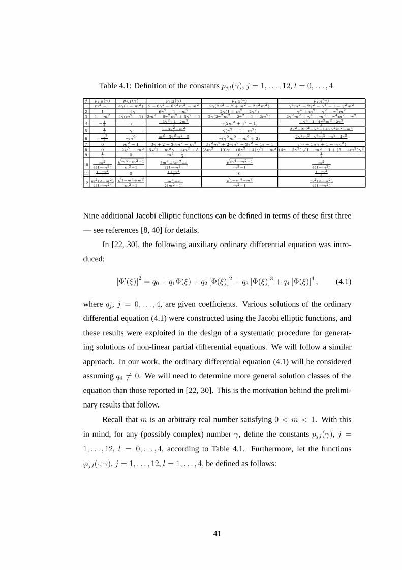
Table 4.1: Definition of the constantspj,l(γ), j = 1, . . . , 12, l = 0, . . . , 4.
j pj,0(γ) pj,1(γ) pj,2(γ) pj,3(γ) pj,4(γ)
1 m2− 1 4γ(1 − m2) 2 − 6γ2 + 6γ2m2
− m2 2γ(2γ2− 2 + m2
− 2γ2m2) γ4m2 + 2γ2− γ4
− 1 − γ2m2
2 1 −4γ 6γ2− 1 − m2 2γ(1 + m2
− 2γ2) γ4 + m2− γ2
− γ2m2
3 1 − m2 4γ(m2− 1) 2m2
− 6γ2m2 + 6γ2− 1 2γ(2γ2m2
− 2γ2 + 1 − 2m2) 2γ2m2 + γ4− m2
− γ4m2− γ2
4 −14
γ−3γ2+1−2m2
2γ(2m2 + γ2
− 1) −γ4−1−4γ2m2+2γ2
4
5 −14
γ1−3γ2+m2
2γ(γ2
− 1 − m2) 2γ2+2m2−γ4
−1+2γ2m2−m4
4
6 −m2
4γm2 m2
−3γ2m2−2
2γ(γ2m2
− m2 + 2) 2γ2m2−γ4m2
−m2−4γ2
47 0 m2
− 1 3γ + 2 − 3γm2− m2 3γ2m2 + 2γm2
− 3γ2− 4γ − 1 γ(γ + 1)(γ + 1 − γm2)
8 0 −2p
1 − m2 6p
1 − m2γ − 4m2 + 5 (8m2− 10)γ − (6γ2 + 4)
p
1 − m2 (4γ + 2γ3)p
1 − m2 + 1 + (5 − 4m2)γ2
9 14
0 −m2 + 12
0 14
10 m2
4(1−m2)
q
m4−m2+1
m2−1
2m4−3m2+4
2(1−m2)
q
m4−m2+1
m2−1
m2
4(1−m2)
11 1−m2
40 1+m2
20 1−m2
4
12 m2(2−m2)
4(1−m2)
q
1−m4+m2
m2−1
m4−4
2(m2−1)
q
1−m4+m2
m2−1
m2(2−m2)
4(1−m2)
Nine additional Jacobi elliptic functions can be defined in terms of these first three
— see references [8, 40] for details.
In [22, 30], the following auxiliary ordinary differentialequation was intro-
duced:
[Φ′(ξ)]2
= q0 + q1Φ(ξ) + q2 [Φ(ξ)]2 + q3 [Φ(ξ)]3 + q4 [Φ(ξ)]4 , (4.1)
whereqj , j = 0, . . . , 4, are given coefficients. Various solutions of the ordinary
differential equation (4.1) were constructed using the Jacobi elliptic functions, and
these results were exploited in the design of a systematic procedure for generat-
ing solutions of non-linear partial differential equations. We will follow a similar
approach. In our work, the ordinary differential equation (4.1) will be considered
assumingq4 6= 0. We will need to determine more general solution classes of the
equation than those reported in [22, 30]. This is the motivation behind the prelimi-
nary results that follow.
Recall thatm is an arbitrary real number satisfying0 < m < 1. With this
in mind, for any (possibly complex) numberγ, define the constantspj,l(γ), j =
1, . . . , 12, l = 0, . . . , 4, according to Table 4.1. Furthermore, let the functions
ϕj,l(·, γ), j = 1, . . . , 12, l = 1, . . . , 4, be defined as follows:
41
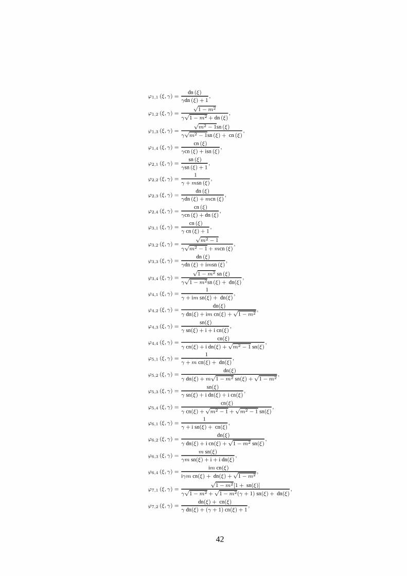
ϕ1,1 (ξ, γ) =dn(ξ)
γdn(ξ) + 1,
ϕ1,2 (ξ, γ) =
√1 −m2
γ√
1 −m2 + dn(ξ),
ϕ1,3 (ξ, γ) =
√m2 − 1sn(ξ)
γ√m2 − 1sn(ξ) + cn(ξ)
,
ϕ1,4 (ξ, γ) =cn(ξ)
γcn(ξ) + isn(ξ),
ϕ2,1 (ξ, γ) =sn(ξ)
γsn(ξ) + 1,
ϕ2,2 (ξ, γ) =1
γ +msn(ξ),
ϕ2,3 (ξ, γ) =dn(ξ)
γdn(ξ) +mcn(ξ),
ϕ2,4 (ξ, γ) =cn(ξ)
γcn(ξ) + dn(ξ),
ϕ3,1 (ξ, γ) =cn(ξ)
γ cn(ξ) + 1,
ϕ3,2 (ξ, γ) =
√m2 − 1
γ√m2 − 1 +mcn(ξ)
,
ϕ3,3 (ξ, γ) =dn(ξ)
γdn(ξ) + imsn(ξ),
ϕ3,4 (ξ, γ) =
√1 −m2 sn(ξ)
γ√
1 −m2sn(ξ) + dn(ξ),
ϕ4,1 (ξ, γ) =1
γ + im sn(ξ) + dn(ξ),
ϕ4,2 (ξ, γ) =dn(ξ)
γ dn(ξ) + im cn(ξ) +√
1 −m2,
ϕ4,3 (ξ, γ) =sn(ξ)
γ sn(ξ) + i + i cn(ξ),
ϕ4,4 (ξ, γ) =cn(ξ)
γ cn(ξ) + i dn(ξ) +√m2 − 1 sn(ξ)
,
ϕ5,1 (ξ, γ) =1
γ +m cn(ξ) + dn(ξ),
ϕ5,2 (ξ, γ) =dn(ξ)
γ dn(ξ) +m√
1 −m2 sn(ξ) +√
1 −m2,
ϕ5,3 (ξ, γ) =sn(ξ)
γ sn(ξ) + i dn(ξ) + i cn(ξ),
ϕ5,4 (ξ, γ) =cn(ξ)
γ cn(ξ) +√m2 − 1 +
√m2 − 1 sn(ξ)
,
ϕ6,1 (ξ, γ) =1
γ + i sn(ξ) + cn(ξ),
ϕ6,2 (ξ, γ) =dn(ξ)
γ dn(ξ) + i cn(ξ) +√
1 −m2 sn(ξ),
ϕ6,3 (ξ, γ) =m sn(ξ)
γm sn(ξ) + i + i dn(ξ),
ϕ6,4 (ξ, γ) =im cn(ξ)
iγm cn(ξ) + dn(ξ) +√
1 −m2,
ϕ7,1 (ξ, γ) =
√1 −m2[1 + sn(ξ)]
γ√
1 −m2 +√
1 −m2(γ + 1) sn(ξ) + dn(ξ),
ϕ7,2 (ξ, γ) =dn(ξ) + cn(ξ)
γ dn(ξ) + (γ + 1) cn(ξ) + 1,
42
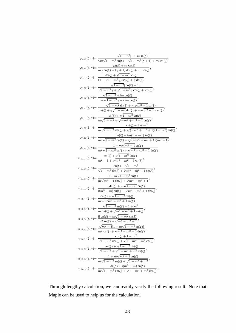
ϕ7,3 (ξ, γ)=
√1 −m2[1 +m sn(ξ)]
γm√
1 −m2 sn(ξ) +√
1 −m2(γ + 1) +mi cn(ξ),
ϕ7,4 (ξ, γ)=dn(ξ) +m cn(ξ)
mγ cn(ξ) + (γ + 1) dn(ξ) + im sn(ξ),
ϕ8,1 (ξ, γ)=dn(ξ) +
√1 −m2 sn(ξ)
(1 +√
1 −m2γ) sn(ξ) + γ dn(ξ),
ϕ8,2 (ξ, γ)=
√1 −m2[ cn(ξ) + 1]√
1 −m2γ +√
1 −m2γ cn(ξ) + cn(ξ),
ϕ8,3 (ξ, γ)=
√1 −m2 + im cn(ξ)
1 +√
1 −m2γ + iγm cn(ξ),
ϕ8,4 (ξ, γ)=
√1 −m2 dn(ξ) +m
√m2 − 1 sn(ξ)
dn(ξ) + γ√
1 −m2 dn(ξ) +m√m2 − 1γ sn(ξ)
,
ϕ9,1 (ξ, γ)=sn(ξ) +
√1 −m2 dn(ξ)
m√
2 −m2 +√−m4 +m2 + 1 cn(ξ)
,
ϕ9,2 (ξ, γ)=cn(ξ) − 1 +m2
m√
2 −m2 dn(ξ) +p
(−m4 +m2 + 1)(1 −m2) sn(ξ),
ϕ9,3 (ξ, γ)=dn(ξ) + im(1 −m2) sn(ξ)
m2√
2 −m2 cn(ξ) +p
(−m4 +m2 + 1)(m2 − 1),
ϕ9,4 (ξ, γ)=1 +m
√m2 − 1 cn(ξ)
m2√
2 −m2 sn(ξ) +√m4 −m2 − 1 dn(ξ)
,
ϕ10,1 (ξ, γ)=cn(ξ) +
√1 −m2 dn(ξ)
m2 − 1 +√m4 −m2 + 1 cn(ξ)
,
ϕ10,2 (ξ, γ)=sn(ξ) +
√1 −m2
√1 −m2 dn(ξ) +
√m4 −m2 + 1 sn(ξ)
,
ϕ10,3 (ξ, γ)=1 +m
√1 −m2 sn(ξ)
m√m2 − 1 cn(ξ) +
√m4 −m2 + 1
,
ϕ10,4 (ξ, γ)=dn(ξ) +m
√1 −m2 cn(ξ)
i(m3 −m) sn(ξ) +√m4 −m2 + 1 dn(ξ)
,
ϕ11,1 (ξ, γ)=cn(ξ) +
√1 −m2 dn(ξ)
m+√m4 −m2 + 1 sn(ξ)
,
ϕ11,2 (ξ, γ)=
√1 −m2 sn(ξ) − 1 +m2
m dn(ξ) +√m4 −m2 + 1 cn(ξ)
,
ϕ11,3 (ξ, γ)=i[ dn(ξ) +m
√1 −m2 cn(ξ)]
m2 sn(ξ) +√m4 −m2 + 1
,
ϕ11,4 (ξ, γ)=
√m2 − 1[1 +m
√1 −m2 sn(ξ)]
m2 cn(ξ) +√m4 −m2 + 1 dn(ξ)
,
ϕ12,1 (ξ, γ)=cn(ξ) + 1 −m2
√1 −m2 dn(ξ) +
√1 −m4 +m2 cn(ξ)
,
ϕ12,2 (ξ, γ)=sn(ξ) +
√1 −m2 dn(ξ)√
1 −m2 +√
1 −m4 +m2 sn(ξ),
ϕ12,3 (ξ, γ)=1 +m
√m2 − 1 cn(ξ)
m√
1 −m2 sn(ξ) +√
1 −m4 +m2,
ϕ12,4 (ξ, γ)=dn(ξ) + i(m3 −m) sn(ξ)
m√
1 −m2 cn(ξ) +√
1 −m4 +m2 dn(ξ).
Through lengthy calculation, we can readily verify the following result. Note that
Maple can be used to help us for the calculation.
43
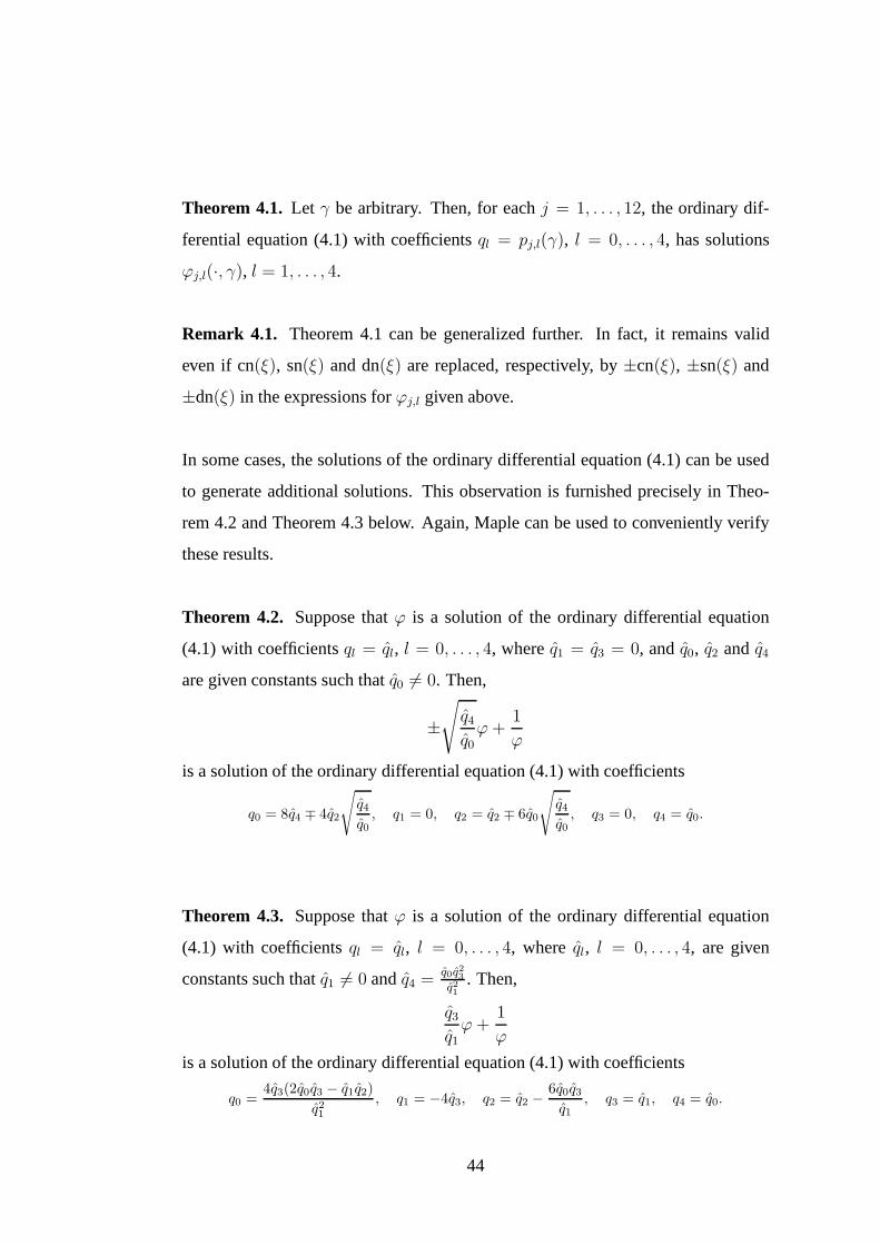
Theorem 4.1. Let γ be arbitrary. Then, for eachj = 1, . . . , 12, the ordinary dif-
ferential equation (4.1) with coefficientsql = pj,l(γ), l = 0, . . . , 4, has solutions
ϕj,l(·, γ), l = 1, . . . , 4.
Remark 4.1. Theorem 4.1 can be generalized further. In fact, it remains valid
even if cn(ξ), sn(ξ) and dn(ξ) are replaced, respectively, by±cn(ξ), ±sn(ξ) and
±dn(ξ) in the expressions forϕj,l given above.
In some cases, the solutions of the ordinary differential equation (4.1) can be used
to generate additional solutions. This observation is furnished precisely in Theo-
rem 4.2 and Theorem 4.3 below. Again, Maple can be used to conveniently verify
these results.
Theorem 4.2. Suppose thatϕ is a solution of the ordinary differential equation
(4.1) with coefficientsql = ql, l = 0, . . . , 4, whereq1 = q3 = 0, andq0, q2 and q4
are given constants such thatq0 6= 0. Then,
±√q4q0ϕ+
1
ϕ
is a solution of the ordinary differential equation (4.1) with coefficients
q0 = 8q4 ∓ 4q2
√q4
q0, q1 = 0, q2 = q2 ∓ 6q0
√q4
q0, q3 = 0, q4 = q0.
Theorem 4.3. Suppose thatϕ is a solution of the ordinary differential equation
(4.1) with coefficientsql = ql, l = 0, . . . , 4, where ql, l = 0, . . . , 4, are given
constants such thatq1 6= 0 andq4 =q0q23q21
. Then,
q3q1ϕ+
1
ϕ
is a solution of the ordinary differential equation (4.1) with coefficients
q0 =4q3(2q0q3 − q1q2)
q21
, q1 = −4q3, q2 = q2 −6q0q3
q1, q3 = q1, q4 = q0.
44
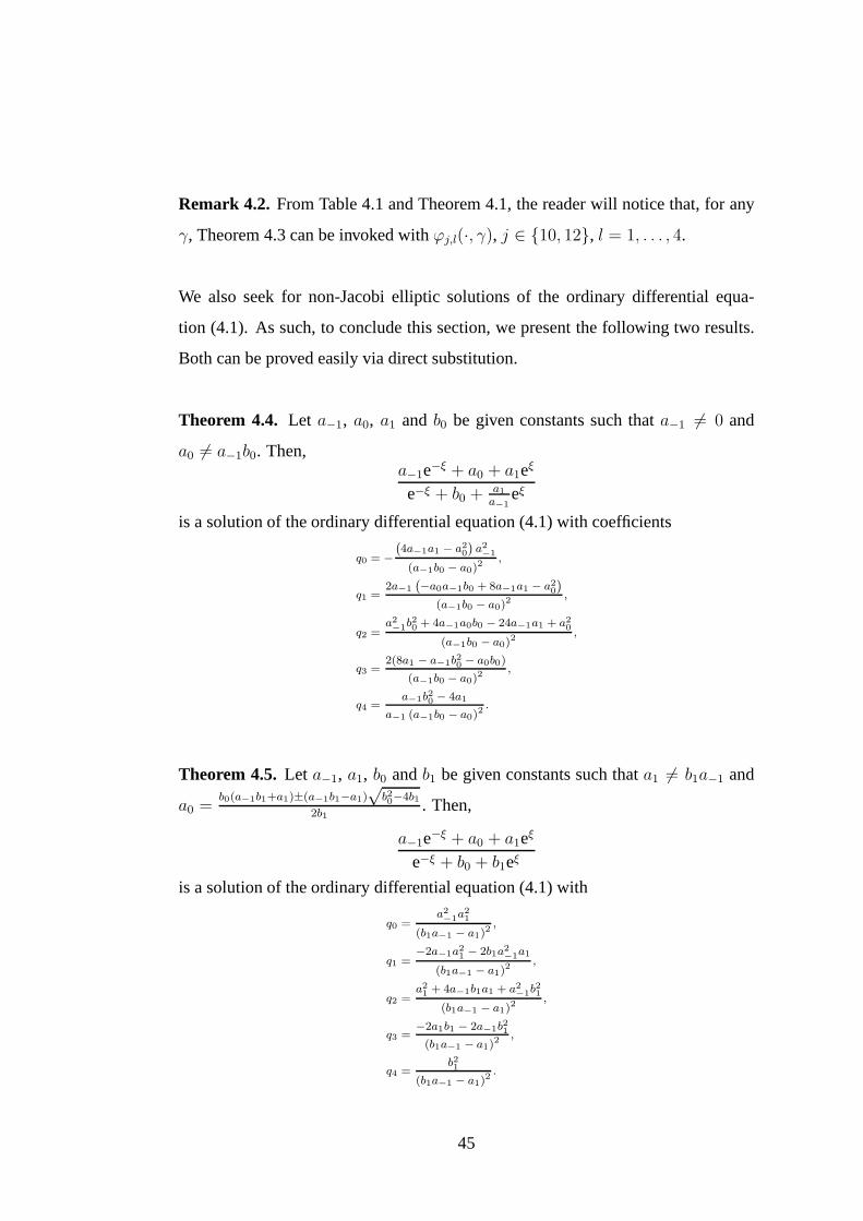
Remark 4.2. From Table 4.1 and Theorem 4.1, the reader will notice that, for any
γ, Theorem 4.3 can be invoked withϕj,l(·, γ), j ∈ {10, 12}, l = 1, . . . , 4.
We also seek for non-Jacobi elliptic solutions of the ordinary differential equa-
tion (4.1). As such, to conclude this section, we present thefollowing two results.
Both can be proved easily via direct substitution.
Theorem 4.4. Let a−1, a0, a1 and b0 be given constants such thata−1 6= 0 and
a0 6= a−1b0. Then,a−1e−ξ + a0 + a1eξ
e−ξ + b0 + a1a−1
eξ
is a solution of the ordinary differential equation (4.1) with coefficients
q0 = −`
4a−1a1 − a20´
a2−1
(a−1b0 − a0)2,
q1 =2a−1
`
−a0a−1b0 + 8a−1a1 − a20´
(a−1b0 − a0)2,
q2 =a2−1b
20 + 4a−1a0b0 − 24a−1a1 + a20
(a−1b0 − a0)2,
q3 =2(8a1 − a−1b20 − a0b0)
(a−1b0 − a0)2,
q4 =a−1b20 − 4a1
a−1 (a−1b0 − a0)2.
Theorem 4.5. Let a−1, a1, b0 andb1 be given constants such thata1 6= b1a−1 and
a0 =b0(a−1b1+a1)±(a−1b1−a1)
√b20−4b1
2b1. Then,
a−1e−ξ + a0 + a1eξ
e−ξ + b0 + b1eξ
is a solution of the ordinary differential equation (4.1) with
q0 =a2−1a
21
(b1a−1 − a1)2,
q1 =−2a−1a21 − 2b1a2−1a1
(b1a−1 − a1)2,
q2 =a21 + 4a−1b1a1 + a2
−1b21
(b1a−1 − a1)2,
q3 =−2a1b1 − 2a−1b21
(b1a−1 − a1)2,
q4 =b21
(b1a−1 − a1)2.
45
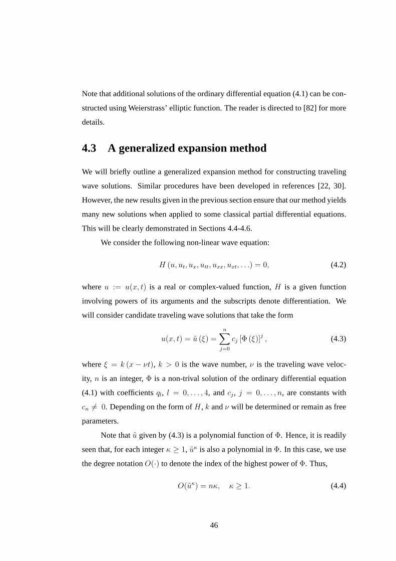
Note that additional solutions of the ordinary differential equation (4.1) can be con-
structed using Weierstrass’ elliptic function. The readeris directed to [82] for more
details.
4.3 A generalized expansion method
We will briefly outline a generalized expansion method for constructing traveling
wave solutions. Similar procedures have been developed in references [22, 30].
However, the new results given in the previous section ensure that our method yields
many new solutions when applied to some classical partial differential equations.
This will be clearly demonstrated in Sections 4.4-4.6.
We consider the following non-linear wave equation:
H (u, ut, ux, utt, uxx, uxt, . . .) = 0, (4.2)
whereu := u(x, t) is a real or complex-valued function,H is a given function
involving powers of its arguments and the subscripts denotedifferentiation. We
will consider candidate traveling wave solutions that takethe form
u(x, t) = u (ξ) =
n∑
j=0
cj [Φ (ξ)]j , (4.3)
whereξ = k (x− νt), k > 0 is the wave number,ν is the traveling wave veloc-
ity, n is an integer,Φ is a non-trival solution of the ordinary differential equation
(4.1) with coefficientsql, l = 0, . . . , 4, andcj, j = 0, . . . , n, are constants with
cn 6= 0. Depending on the form ofH, k andν will be determined or remain as free
parameters.
Note thatu given by (4.3) is a polynomial function ofΦ. Hence, it is readily
seen that, for each integerκ ≥ 1, uκ is also a polynomial inΦ. In this case, we use
the degree notationO(·) to denote the index of the highest power ofΦ. Thus,
O(uκ) = nκ, κ ≥ 1. (4.4)
46
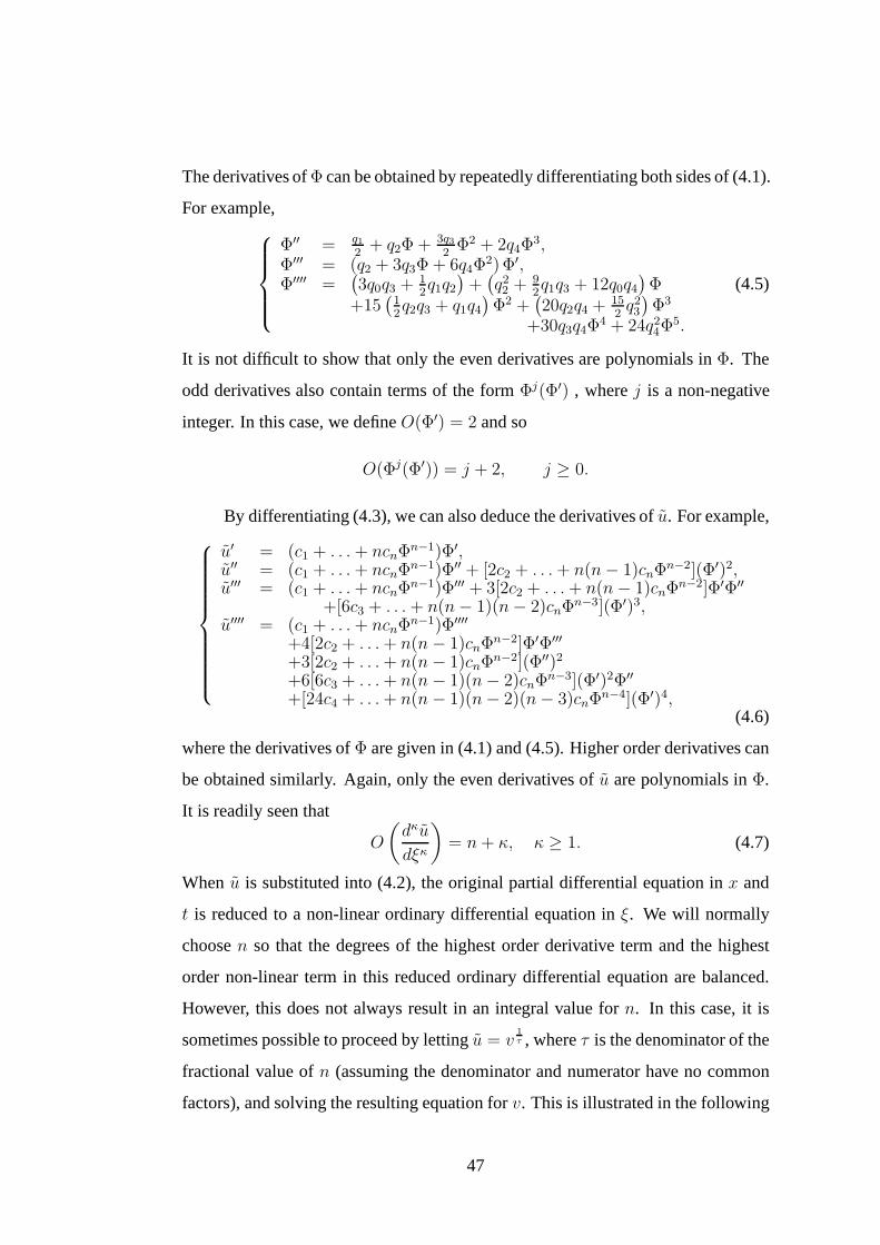
The derivatives ofΦ can be obtained by repeatedly differentiating both sides of(4.1).
For example,
Φ′′ = q12
+ q2Φ + 3q32
Φ2 + 2q4Φ3,
Φ′′′ = (q2 + 3q3Φ + 6q4Φ2)Φ′,
Φ′′′′ =(3q0q3 + 1
2q1q2
)+(q22 + 9
2q1q3 + 12q0q4
)Φ
+15(
12q2q3 + q1q4
)Φ2 +
(20q2q4 + 15
2q23
)Φ3
+30q3q4Φ4 + 24q2
4Φ5.
(4.5)
It is not difficult to show that only the even derivatives are polynomials inΦ. The
odd derivatives also contain terms of the formΦj(Φ′) , wherej is a non-negative
integer. In this case, we defineO(Φ′) = 2 and so
O(Φj(Φ′)) = j + 2, j ≥ 0.
By differentiating (4.3), we can also deduce the derivatives of u. For example,
u′ = (c1 + . . .+ ncnΦn−1)Φ′,
u′′ = (c1 + . . .+ ncnΦn−1)Φ′′ + [2c2 + . . .+ n(n− 1)cnΦ
n−2](Φ′)2,u′′′ = (c1 + . . .+ ncnΦ
n−1)Φ′′′ + 3[2c2 + . . .+ n(n− 1)cnΦn−2]Φ′Φ′′
+[6c3 + . . .+ n(n− 1)(n− 2)cnΦn−3](Φ′)3,
u′′′′ = (c1 + . . .+ ncnΦn−1)Φ′′′′
+4[2c2 + . . .+ n(n− 1)cnΦn−2]Φ′Φ′′′
+3[2c2 + . . .+ n(n− 1)cnΦn−2](Φ′′)2
+6[6c3 + . . .+ n(n− 1)(n− 2)cnΦn−3](Φ′)2Φ′′
+[24c4 + . . .+ n(n− 1)(n− 2)(n− 3)cnΦn−4](Φ′)4,
(4.6)
where the derivatives ofΦ are given in (4.1) and (4.5). Higher order derivatives can
be obtained similarly. Again, only the even derivatives ofu are polynomials inΦ.
It is readily seen that
O
(dκu
dξκ
)= n+ κ, κ ≥ 1. (4.7)
When u is substituted into (4.2), the original partial differential equation inx and
t is reduced to a non-linear ordinary differential equation in ξ. We will normally
choosen so that the degrees of the highest order derivative term and the highest
order non-linear term in this reduced ordinary differential equation are balanced.
However, this does not always result in an integral value forn. In this case, it is
sometimes possible to proceed by lettingu = v1τ , whereτ is the denominator of the
fractional value ofn (assuming the denominator and numerator have no common
factors), and solving the resulting equation forv. This is illustrated in the following
47
example.
Example 4.1.Consider the following Boussinesq-type equation:
utt − uxx + uxxxx + (u5 − u3)xx = 0.
By lettingu(x, t) = u(k(x− νt)), the above partial differential equation is reduced
to the following ordinary differential equation:
ν2u′′ − u′′ + k2u′′′′ + (u5 − u3)′′ = 0.
Integrating twice yields
ν2u− u+ k2u′′ + u5 − u3 = 0. (4.8)
Here, the highest order non-linear term isu5, and the highest order derivative term
is u′′. Balancing these two terms using (4.4) and (4.7) gives5n = n + 2, or n = 12.
Settingu = v12 , (4.8) becomes
(ν2 − 1)v2 +k2
4[2vv′′ − (v′)2] + v4 − v3 = 0. (4.9)
Now, balancing(v′)2 andv4 givesn = 1. Hence, we can search for traveling wave
solutions of (4.9) which take the formv (k(x− νt)) = c0 + c1Φ (k(x− νt)), for
constantsc0 andc1. If such av can be determined, then it is easy to deriveu. �
It is noted in Example 4.1 that substitutingu into (4.2) yields a non-linear ordinary
differential equation inξ. When the derivatives ofu are substituted into this reduced
ordinary differential equation, we will obtain a linear combination ofΦj(Φ′)l, where
j ≥ 0 is an integer andl ∈ {0, 1}. If ν, k, andcj, j = 0, . . . , n, andqj , j = 0, . . . , 4,
can be chosen to make each coefficient in this linear combination zero, then the re-
sulting u will satisfy the original partial differential equation (4.2). However, in
this procedure, we sometimes end up withcj = 0, j = 0, . . . , n (we encounter
this in Section 4.6). In this case, we can use the following alternative solution form
proposed in [22]:
u(ξ) = c0 +n∑
j=1
cj[Φ(ξ)]j + Cj[Φ(ξ)]j−1Φ′(ξ)
[µΦ(ξ) + 1]j, (4.10)
48
wherecj (j = 0, . . . , n), Cj (j = 1, . . . , n) andµ are constants.
In [7, 30], the solutions to the reduced ordinary differential equation are rep-
resented by
u(ξ) =n∑
j=−ncj[Φ(ξ)
]j+
Φ′(ξ)[Φ(ξ)
]2
(n+1∑
j=−nCj[Φ(ξ)
]j). (4.11)
However, the degree ofu given in (4.11) isn + 1. Hence,Cn+1 = 0. Thus, it
becomes
u(ξ) =
n∑
j=−ncj[Φ(ξ)
]j+
Φ′(ξ)[Φ(ξ)
]2
(n∑
j=−nCj[Φ(ξ)
]j). (4.12)
In (4.12), there are4n + 2 variables which need to be determined, while there are
only 2n + 2 variables (cj , j = 0, . . . , n, Cj, j = 1, . . . , n, andµ) in (4.10). Note
that, in (4.12),q1 = q3 = 0 is required. Hence, combining Theorem 4.2 and
expression (4.10) withµ = 0, we can derive the same result as the ones derived
from (4.12). But, (4.10) is much more easy than (4.12) for calculations.
Notice that each of the Jacobi elliptic solutions of the ordinary differential
equation (4.1) reported in [22, 64, 71] can be written as a scalar multiple of some
ϕj,l(·, 0), j ∈ {1, . . . , 6}, l ∈ {1, . . . , 4}. Hence, by applying our expansion
method with (4.3) and Theorem 4.1 to a non-linear partial differential equation, we
can replicate every Jacobi elliptic solution obtained using the methods presented
in [64, 71]. Applying our expansion method with (4.10) and Theorem 4.1 to a
non-linear partial differential equation, we can obtain all Jacobi elliptic solutions
obtained using the method presented in [22]. Similarly, each Jacobi elliptic solu-
tion of the ordinary differential equation (4.1) reported in [30, 36] withω = 1 can
be written as a scalar multiple of someϕj,l(·, 0), j ∈ {1, . . . , 6}, l ∈ {1, . . . , 4}.
It is also evident that, for the special caseµ = 0, using our expansion method
with (4.10) and Theorem 4.1 and Theorem 4.2, we can recover every Jacobi elliptic
solution obtained using the method of [30, 106]. Hence, by virtue of the new results
in Section 4.2, our method is a significant generalization ofthe work reported in
[7, 22, 30, 36, 42, 64, 71, 106].
49
4.4 Traveling wave solutions for the Boussinesq equa-tion
Consider the Boussinesq equation
utt + α1uxx + α2uxxxx + α3
(u2)xx
= 0, (4.13)
whereu := u (x, t) is a real-valued function. Lettingu(x, t) = u(ξ), whereξ is as
defined in Section 4.3, (4.13) becomes an ordinary differential equation
ν2u′′ + α1u′′ + α2k
2u′′′′ + α3
(u2)′′
= 0. (4.14)
Now, let us solve the following ordinary differential equation:
β1Ψ′′(ξ) + β2Ψ
′′′′(ξ) + β3
[Ψ2(ξ)
]′′= 0, (4.15)
where constantsβj, j = 1, 2, 3, are non-zero. Balancing[Ψ2(ξ)]′′ andΨ′′′′(ξ) gives
2n+2 = n+4, orn = 2. Hence, we will search for candidate solutions of the form
Ψ(ξ) = c0 + c1Φ(ξ) + c2 [Φ(ξ)]2 , (4.16)
wherec2 6= 0 andΦ satisfies the ordinary differential equation (4.1) with coeffi-
cientsqj, j = 0, . . . , 4. Substituting (4.16) into (4.15) and using (4.1) and (4.5)-
(4.6), we obtain the following sufficient conditions forΨ to satisfy (4.15):
c0 =3β2q
23 − 16β2q2q4 − 4β1q4
8β3q4,
c1 = −3β2q3β3
,
c2 = −6β2q4β3
,
q1 =q3 (4q2q4 − q2
3)
8q24
.
(4.17)
That is, if a solutionΦ of the ordinary differential equation (4.1) with coefficients
satisfyingq1 =q3(4q2q4−q23)
8q24andq4 6= 0 can be found, then
Ψ(ξ) = c0 + c1Φ(ξ) + c2 [Φ(ξ)]2 , (4.18)
50
wherec0, c1, c2 are as defined in (4.17), is a solution of the ordinary differential
equation (4.15). Now, we generalize this solution form further. Note that, ifq1 =
q3 = 0, then (4.18) reduces to
Ψ(ξ) = −4β2q2+β1
2β3− 6β2q4
β3[Φ(ξ)]2 . (4.19)
If q0 6= 0, then using Theorem 4.2 with (4.19) gives the following solution form for
equation (4.15):
Ψ(ξ) = −4β2q2 + β1
2β3− 6β2q4
β3[Φ(ξ)]2 − 6β2q0
β3 [Φ(ξ)]2. (4.20)
Furthermore, note that (4.18) can be rewritten as
Ψ(ξ) =3β2q
23 − 8β2q2q4 − 2β1q4
4β3q4− 6β2q4
β3
[Φ(ξ) +
q34q4
]2. (4.21)
The solution forms (4.20) and (4.21) provide motivation forthe following more
general candidate solution:
Ψ(ξ) =3β2q
23 − 8β2q2q4 − 2β1q4
4β3q4− 6β2q4
β3
[Φ(ξ)+
q34q4
]2+
d[Φ(ξ) + q3
4q4
]2 , (4.22)
whered is a constant. By substituting (4.22) into (4.15), the valueof d can be de-termined. We summarize our results in the form of the following theorem.
Theorem 4.6. For eachj = 1, 2, let εj ∈ {0, 1}. Suppose thatΦ is a solutionof the ordinary differential equation (4.1) with coefficients qj , j = 0, . . . , 4, satisfy-
ing q4 6= 0 andq1 =q3(4q2q4−q23)
8q24. Then,
Ψ1(ξ, β1, β2, β3) =3β2q
23 − 8β2q2q4 − 2β1q4
4β3q4− ε1
6β2q4
β3
[Φ(ξ) +
q3
4q4
]2
+ ε23β2(16q
23q2q4 − 5q4
3 − 256q34q0)
128β3q34
[Φ(ξ) + q3
4q4
]2
is a solution of the ordinary differential equation (4.15).
Remark 4.3.Ψ1 includes both (4.18) and (4.20) as special cases.
Remark 4.4. When q1 = q3 = 0, using the method proposed in [42], where
51
n∑j=−n
cj[Φ(ξ)
]jhas been used, the same results will be derived asΨ1 with q1 =
q3 = 0.
Applying Theorem 4.6 and using the solutions of (4.1) given in Theorems 4.1,
4.4 and 4.5, we can deduce many solutions for equation (4.15). Let the functions
ψj(ξ, β1, β2, β3), j = 1, . . . , 26, be defined as follows:
ψ1(ξ, β1, β2, β3) =2β2 − β1
2β3− 3β2
2β3
"
ε1
„−e−ξ ±q
λ21 − 4λ2 + λ2eξ
e−ξ + λ1 + λ2eξ
«2
+ ε2
„
e−ξ + λ1 + λ2eξ
−e−ξ ±q
λ21 − 4λ2 + λ2eξ
«2#
,
ψ2(ξ, β1, β2, β3) = − 2β2 + β1
2β3− 3β2
2β3
"
ε1
„ sin(ξ) ±q
1 − λ23
cos(ξ) + λ3
«2
+ ε2
„
cos(ξ) + λ3
sin(ξ) ±q
1 − λ23
«2#
,
ψ3(ξ, β1, β2, β3) =4β2
`
m2 + 1´
− β1
2β3− 6β2
β3
ˆ
ε1m2sn2(ξ) + ε2sn−2(ξ)
˜
,
ψ4(ξ, β1, β2, β3) =4β2
`
m2 − 2´
− β1
2β3+
6β2
β3
»
ε1dn2(ξ) +1 −m2
dn2(ξ)
–
,
ψ5(ξ, β1, β2, β3) =4β2
`
m2 − 2´
− β1
2β3− 6β2
β3
»
ε1cn2(ξ)
sn2(ξ)+
(1 −m2)sn2(ξ)
cn2(ξ)
–
,
ψ6(ξ, β1, β2, β3) =4β2
`
m2 + 1´
− β1
2β3− 6β2
β3
»
m2 cn2(ξ)
dn2(ξ)+
dn2(ξ)
cn2(ξ)
–
,
ψ7(ξ, β1, β2, β3) = −β1 + 4β2
`
2m2 − 1´
2β3− 6β2
β3
»
−m2cn2(ξ) +1 −m2
cn2(ξ)
–
,
ψ8(ξ, β1, β2, β3) = −β1 + 4β2
`
2m2 − 1´
2β3− 6β2
β3
»
dn2(ξ)
sn2(ξ)+m2(m2 − 1)sn2(ξ)
dn2(ξ)
–
,
ψ9(ξ, β1, β2, β3) =2β2
`
2m2 − 1´
− β1
2β3− 3β2[1 − cn(ξ)]
2β3[1 + cn(ξ)],
ψ10(ξ, β1, β2, β3) =2β2
`
2m2 − 1´
− β1
2β3− 3β2[dn(ξ) −
√1 −m2sn(ξ)]
2β3[dn(ξ) +√
1 −m2sn(ξ)],
ψ11(ξ, β1, β2, β3) = −β1 + 2β2
`
m2 + 1´
2β3+
3β2(1 −m2)[1 −msn(ξ)]
2β3[1 +msn(ξ)],
ψ12(ξ, β1, β2, β3) = −β1 + 2β2
`
m2 + 1´
2β3− 3β2(1 −m2)[1 − sn(ξ)]
2β3[1 + sn(ξ)],
ψ13(ξ, β1, β2, β3) = −β1 + 2β2
`
m2 + 1´
2β3− 3β2(1 −m2)[dn(ξ) − cn(ξ)]
2β3[dn(ξ) + cn(ξ)],
ψ14(ξ, β1, β2, β3) = −β1 + 2β22
`
m2 + 1´
2β3+
3β2(m2 − 1)[mcn(ξ) − dn(ξ)]
2β3[mcn(ξ) + dn(ξ)],
52
ψ15(ξ, β1, β2, β3) =−β1 + 2β2
`
m2 − 2´
2β3− 3β2m2[dn(ξ) −
√1 −m2]
2β3[dn(ξ) +√
1 −m2],
ψ16(ξ, β1, β2, β3) =−β1 + 2β2
`
m2 − 2´
2β3− 3β2m2[1 − dn(ξ)]
2β3[1 + dn(ξ)],
ψ17(ξ, β1, β2, β3) =−β1 + β2
`
2m2 + 12m + 2´
2β3+
3β2(m− 1)2
2β3
(
»
1 −√msn(ξ)
1 +√msn(ξ)
–2
+ ε1
»
1 +√msn(ξ)
1 −√msn(ξ)
–2)
,
ψ18(ξ, β1, β2, β3) =−β1 + β2
`
2m2 + 12m + 2´
2β3
+3β2(m− 1)2
2β3
(
»
dn(ξ) −√mcn(ξ)
dn(ξ) +√mcn(ξ)
–2
+ ε1
»
dn(ξ) +√mcn(ξ)
dn(ξ) −√mcn(ξ)
–2)
,
ψ19(ξ, β1, β2, β3) =−β1 + β2(2m2 − 4 + 12√
1 −m2)
2β3
−3β2(1 +√
1 −m2)2
2β3
8
<
:
"
cn(ξ) − 4√
1 −m2sn(ξ)
cn(ξ) + 4√
1 −m2sn(ξ)
#2
+ ε1
"
cn(ξ) + 4√
1 −m2sn(ξ)
cn(ξ) − 4√
1 −m2sn(ξ)
#29
=
;
,
ψ20(ξ, β1, β2, β3) =−β1 + β2(2m2 − 4 − 12√
1 −m2)
2β3
−3β2(1 −√
1 −m2)2
2β3
8
<
:
"
dn(ξ) − 4√
1 −m2
dn(ξ) + 4√
1 −m2
#2
+ ε1
"
dn(ξ) + 4√
1 −m2
dn(ξ) − 4√
1 −m2
#29
=
;
,
ψ21(ξ, β1, β2, β3) =2β2
`
2m2 − 1´
− β1
2β3− 3β2
2β3
"
sn(ξ) +√
1 −m2dn(ξ)
m√
2 −m2 +√−m4 +m2 + 1cn(ξ)
#2
−3β2
2β3ε1
"
m√
2 −m2 +√−m4 +m2 + 1cn(ξ)
sn(ξ) +√
1 −m2dn(ξ)
#2
,
ψ22(ξ, β1, β2, β3) =2β2
`
2m2 − 1´
− β1
2β3− 3β2
2β3
"
cn(ξ) + (m2 − 1)
m√
2 −m2dn(ξ) +p
(−m4 +m2 + 1)(1 −m2)sn(ξ)
#2
−ε13β2
2β3
"
m√
2 −m2dn(ξ) +p
(−m4 +m2 + 1)(1 −m2)sn(ξ)
cn(ξ) + (m2 − 1)
#2
,
ψ23(ξ, β1, β2, β3) =−β1 + 2β2
`
m2 + 1´
2β3+
3β2(m2 − 1)
2β3
"
cn(ξ) +√
1 −m2dn(ξ)
m+√m4 −m2 + 1sn(ξ)
#2
+ε13β2(m2 − 1)
2β3
"
m+√m4 −m2 + 1sn(ξ)
cn(ξ) +√
1 −m2dn(ξ)
#2
,
ψ24(ξ, β1, β2, β3) =−β1 + 2β2
`
m2 + 1´
2β3− 3β2(1 −m2)2
2β3
"
sn(ξ) +√
1 −m2
mdn(ξ) +√m4 −m2 + 1cn(ξ)
#2
−ε13β2
2β3
"
mdn(ξ) +√m4 −m2 + 1cn(ξ)
sn(ξ) +√
1 −m2
#2
,
ψ25(ξ, β1, β2, β3) =−β1 + 2β2
`
m2 + 1´
2β3− 3β2(m2 − 1)
2β3
"
dn(ξ) +√
1 −m2cn(ξ)
m2sn(ξ) +√m4 −m2 + 1
#2
−ε13β2(m2 − 1)
2β3
"
m2sn(ξ) +√m4 −m2 + 1
dn(ξ) +√
1 −m2cn(ξ)
#2
,
ψ26(ξ, β1, β2, β3) =−β1 + 2β2
`
m2 + 1´
2β3+
3β2(1 −m2)2
2β3
"
1 +m√
1 −m2sn(ξ)
m2cn(ξ) +√m4 −m2 + 1dn(ξ)
#2
+ε13β2
2β3
"
m2cn(ξ) +√m4 −m2 + 1dn(ξ)
1 +m√
1 −m2sn(ξ)
#2
,
whereε1, ε2 ∈ {0, 1},m ∈ (0, 1) is the modulus of the Jacobi elliptic functions, and
53

λj , j = 1, 2, 3, are arbitrary real constants satisfyingλ21 ≤ 4λ2 and−1 ≤ λ3 ≤ 1.
Through direct substitution, we can prove the following result.
Theorem 4.7. For eachj = 1, . . . , 26, the functionψj is a solution of the ordi-
nary differential equation (4.15).
Remark 4.5. It follows from Remark 4.1 thatψj , j = 3, . . . , 26, still satisfy equa-
tion (4.15) even if cn(ξ), sn(ξ) and dn(ξ) are replaced, respectively, by±cn(ξ),
±sn(ξ) and±dn(ξ).
Remark 4.6. It is interesting to note that, for eachj ∈ {3, . . . , 26}, the solutionψj
becomes a special case ofψ1 asm→ 1. Similarly, asm→ 0, ψj becomes a special
case ofψ2.
Next, we will make use of the solutionsψj , j = 1, . . . , 26, to derive traveling wave
solutions for the Boussinesq equation (4.13).
For eachj = 1, . . . , 26, let
uj(x, t) := ψj(k(x− νt), α1 + ν2, α2k
2, α3
),
wherek andν are arbitrary real constants. According to Theorem 4.6 and (4.14),
we know that, for eachj = 1, . . . , 26, the functionuj is a solution of the Boussinesq
equation (4.13).
Note that, for some cases, the denominators in the expression of u1 can be
equal to zero at certain points, and thus, such a solution is unbounded. For example,
u1 with ε1 = ε2 = 1 andλ2 6= 0 is unbounded. It is also noted that, for some cases,
the solutionu1 is bounded. For instance,u1 with ε1 = 1, ε2 = 0, 0 ≤ λ2 ≤ λ21/4
andλ1 ≥ 0 is bounded. For the bounded case, clearly, the solutionu1 gives a single
wave that moves in thex-direction with velocityν andu1(x, t) → (2α2k2 − α1 −
ν2)/(2α3) − 3α2k2(ε1 + ε2)/(2α3) ask(x− νt) → ±∞.
To show the physical insight of these solutions, here we chooseα1 = −1,
54
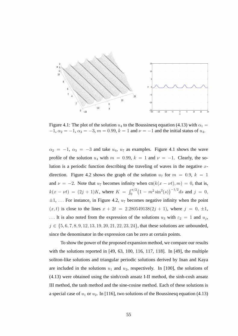
−20
−10
0
10
20
0
2
4
6
8
10−2
02
x
t
u
−20 −15 −10 −5 0 5 10 15 20−15
−10
−5
0
5
10
15
x
u
Figure 4.1: The plot of the solutionu4 to the Boussinesq equation (4.13) withα1 =−1, α2 = −1, α3 = −3,m = 0.99, k = 1 andν = −1 and the initial status ofu4.
α2 = −1, α3 = −3 and takeu4, u7 as examples. Figure 4.1 shows the wave
profile of the solutionu4 with m = 0.99, k = 1 andν = −1. Clearly, the so-
lution is a periodic function describing the traveling of waves in the negativex-
direction. Figure 4.2 shows the graph of the solutionu7 for m = 0.9, k = 1
andν = −2. Note thatu7 becomes infinity when cn(k(x − νt), m) = 0, that is,
k(x − νt) = (2j + 1)K, whereK =∫ π/20
(1 − m2 sin2(s)
)−1/2ds and j = 0,
±1, . . . For instance, in Figure 4.2,u7 becomes negative infinity when the point
(x, t) is close to the linesx + 2t = 2.280549138(2j + 1), wherej = 0, ±1,
. . . It is also noted from the expression of the solutionsu3 with ε2 = 1 anduj,
j ∈ {5, 6, 7, 8, 9, 12, 13, 19, 20, 21, 22, 23, 24}, that these solutions are unbounded,
since the denominator in the expression can be zero at certain points.
To show the power of the proposed expansion method, we compare our results
with the solutions reported in [49, 63, 100, 116, 117, 118]. In [49], the multiple
soliton-like solutions and triangular periodic solutionsderived by Inan and Kaya
are included in the solutionsu1 andu2, respectively. In [100], the solutions of
(4.13) were obtained using the sinh/cosh ansatz I-II method, the sinh-cosh ansatz
III method, the tanh method and the sine-cosine method. Eachof these solutions is
a special case ofu1 or u2. In [116], two solutions of the Boussinesq equation (4.13)
55
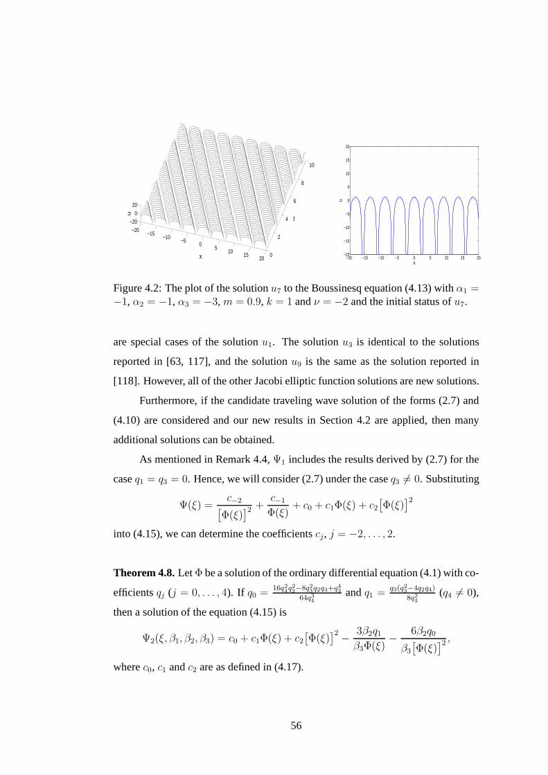
−20−15
−10−5
05
1015
200
2
4
6
8
10
−20
0
20
t
x
u
−20 −15 −10 −5 0 5 10 15 20−20
−15
−10
−5
0
5
10
15
20
x
u
Figure 4.2: The plot of the solutionu7 to the Boussinesq equation (4.13) withα1 =−1, α2 = −1, α3 = −3,m = 0.9, k = 1 andν = −2 and the initial status ofu7.
are special cases of the solutionu1. The solutionu3 is identical to the solutions
reported in [63, 117], and the solutionu9 is the same as the solution reported in
[118]. However, all of the other Jacobi elliptic function solutions are new solutions.
Furthermore, if the candidate traveling wave solution of the forms (2.7) and
(4.10) are considered and our new results in Section 4.2 are applied, then many
additional solutions can be obtained.
As mentioned in Remark 4.4,Ψ1 includes the results derived by (2.7) for the
caseq1 = q3 = 0. Hence, we will consider (2.7) under the caseq3 6= 0. Substituting
Ψ(ξ) =c−2[
Φ(ξ)]2 +
c−1
Φ(ξ)+ c0 + c1Φ(ξ) + c2
[Φ(ξ)
]2
into (4.15), we can determine the coefficientscj, j = −2, . . . , 2.
Theorem 4.8.LetΦ be a solution of the ordinary differential equation (4.1) with co-
efficientsqj (j = 0, . . . , 4). If q0 =16q24q
22−8q23q2q4+q
43
64q34andq1 =
q3(q23−4q2q4)
8q24(q4 6= 0),
then a solution of the equation (4.15) is
Ψ2(ξ, β1, β2, β3) = c0 + c1Φ(ξ) + c2[Φ(ξ)
]2 − 3β2q1β3Φ(ξ)
− 6β2q0
β3
[Φ(ξ)
]2 ,
wherec0, c1 andc2 are as defined in (4.17).
56
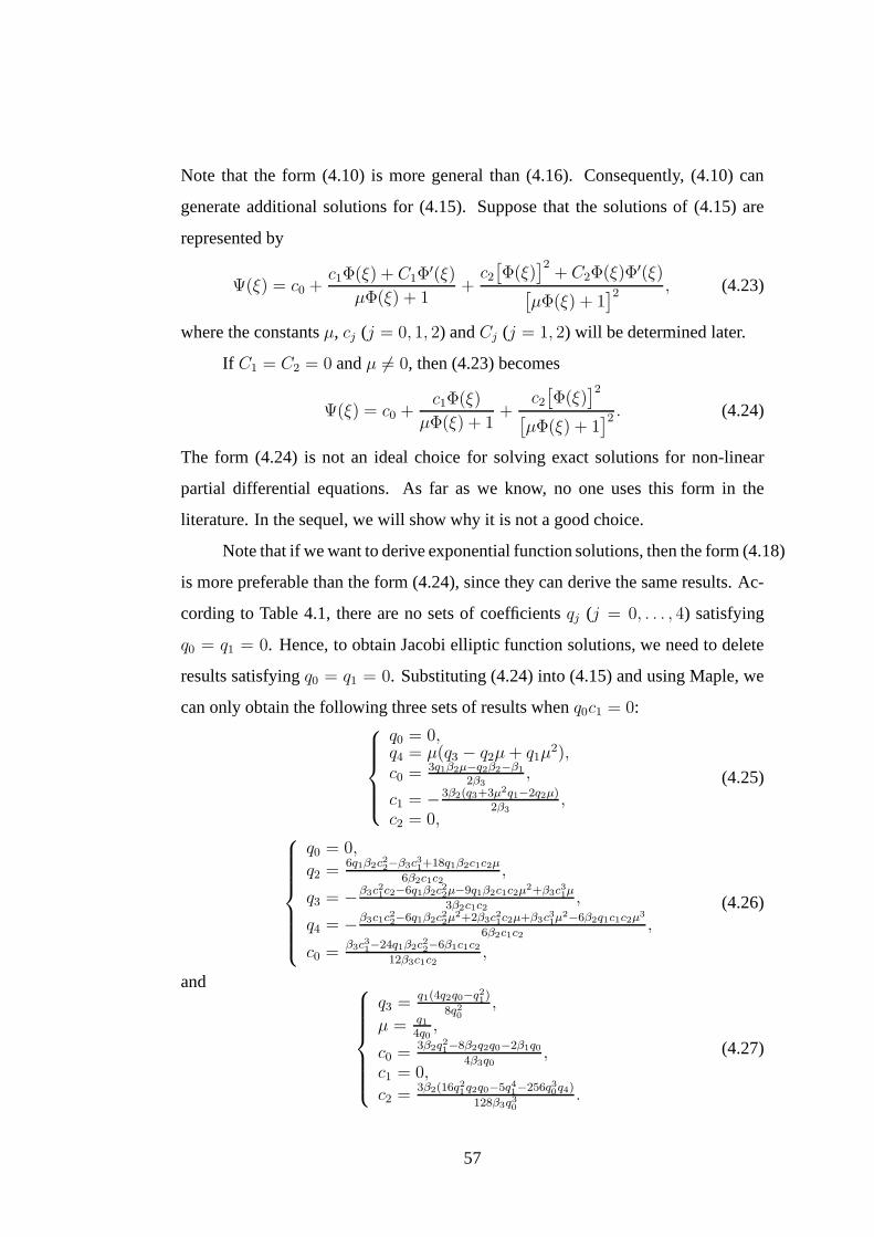
Note that the form (4.10) is more general than (4.16). Consequently, (4.10) can
generate additional solutions for (4.15). Suppose that thesolutions of (4.15) are
represented by
Ψ(ξ) = c0 +c1Φ(ξ) + C1Φ
′(ξ)
µΦ(ξ) + 1+c2[Φ(ξ)
]2+ C2Φ(ξ)Φ′(ξ)
[µΦ(ξ) + 1
]2 , (4.23)
where the constantsµ, cj (j = 0, 1, 2) andCj (j = 1, 2) will be determined later.
If C1 = C2 = 0 andµ 6= 0, then (4.23) becomes
Ψ(ξ) = c0 +c1Φ(ξ)
µΦ(ξ) + 1+
c2[Φ(ξ)
]2[µΦ(ξ) + 1
]2 . (4.24)
The form (4.24) is not an ideal choice for solving exact solutions for non-linear
partial differential equations. As far as we know, no one uses this form in the
literature. In the sequel, we will show why it is not a good choice.
Note that if we want to derive exponential function solutions, then the form (4.18)
is more preferable than the form (4.24), since they can derive the same results. Ac-
cording to Table 4.1, there are no sets of coefficientsqj (j = 0, . . . , 4) satisfying
q0 = q1 = 0. Hence, to obtain Jacobi elliptic function solutions, we need to delete
results satisfyingq0 = q1 = 0. Substituting (4.24) into (4.15) and using Maple, we
can only obtain the following three sets of results whenq0c1 = 0:
q0 = 0,q4 = µ(q3 − q2µ+ q1µ
2),c0 = 3q1β2µ−q2β2−β1
2β3,
c1 = −3β2(q3+3µ2q1−2q2µ)2β3
,c2 = 0,
(4.25)
q0 = 0,
q2 =6q1β2c22−β3c31+18q1β2c1c2µ
6β2c1c2,
q3 = −β3c21c2−6q1β2c22µ−9q1β2c1c2µ2+β3c31µ
3β2c1c2,
q4 = −β3c1c22−6q1β2c22µ2+2β3c21c2µ+β3c31µ
2−6β2q1c1c2µ3
6β2c1c2,
c0 =β3c31−24q1β2c22−6β1c1c2
12β3c1c2,
(4.26)
and
q3 =q1(4q2q0−q21)
8q20,
µ = q14q0,
c0 =3β2q21−8β2q2q0−2β1q0
4β3q0,
c1 = 0,
c2 =3β2(16q21q2q0−5q41−256q30q4)
128β3q30.
(4.27)
57
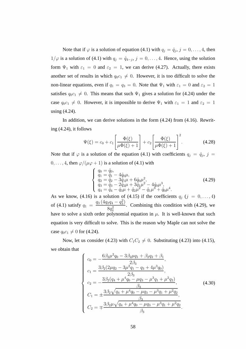
Note that ifϕ is a solution of equation (4.1) withqj = qj , j = 0, . . . , 4, then
1/ϕ is a solution of (4.1) withqj = q4−j , j = 0, . . . , 4. Hence, using the solution
form Ψ1 with ε1 = 0 and ε2 = 1, we can derive (4.27). Actually, there exists
another set of results in whichq0c1 6= 0. However, it is too difficult to solve the
non-linear equations, even ifq1 = q3 = 0. Note thatΨ1 with ε1 = 0 andε2 = 1
satisfiesq0c1 6= 0. This means that suchΨ1 gives a solution for (4.24) under the
caseq0c1 6= 0. However, it is impossible to deriveΨ1 with ε1 = 1 andε2 = 1
using (4.24).
In addition, we can derive solutions in the form (4.24) from (4.16). Rewrit-
ing (4.24), it follows
Ψ(ξ) = c0 + c1
[Φ(ξ)
µΦ(ξ) + 1
]+ c2
[Φ(ξ)
µΦ(ξ) + 1
]2
. (4.28)
Note that ifϕ is a solution of the equation (4.1) with coefficientsqj = qj, j =
0, . . . , 4, thenϕ/(µϕ+ 1) is a solution of (4.1) with
q0 = q0,q1 = q1 − 4q0µ,q2 = q2 − 3q1µ+ 6q0µ
2,q3 = q3 − 2q2µ+ 3q1µ
2 − 4q0µ3,
q4 = q4 − q3µ+ q2µ2 − q1µ
3 + q0µ4.
(4.29)
As we know, (4.16) is a solution of (4.15) if the coefficientsqj (j = 0, . . . , 4)
of (4.1) satisfyq1 =q3 (4q2q4 − q2
3)
8q24
. Combining this condition with (4.29), we
have to solve a sixth order polynomial equation inµ. It is well-known that such
equation is very difficult to solve. This is the reason why Maple can not solve the
caseq0c1 6= 0 for (4.24).
Now, let us consider (4.23) withC1C2 6= 0. Substituting (4.23) into (4.15),
we obtain that
c0 = −6β2µ2q0 − 3β2µq1 + β2q2 + β1
2β3
,
c1 =3β2(2µq2 − 3µ2q1 − q3 + 4µ3q0)
2β3,
c2 = −3β2(q4 + µ4q0 − µq3 − µ3q1 + µ2q2)
β3,
C1 = ±3β2
√q4 + µ4q0 − µq3 − µ3q1 + µ2q2
β3,
C2 = ∓3β2µ√q4 + µ4q0 − µq3 − µ3q1 + µ2q2
β3.
(4.30)
58
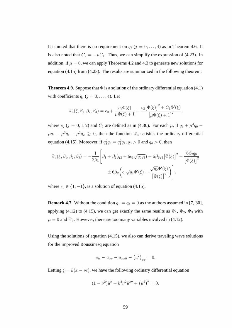
It is noted that there is no requirement onqj (j = 0, . . . , 4) as in Theorem 4.6. It
is also noted thatC2 = −µC1. Thus, we can simplify the expression of (4.23). In
addition, ifµ = 0, we can apply Theorems 4.2 and 4.3 to generate new solutions for
equation (4.15) from (4.23). The results are summarized in the following theorem.
Theorem 4.9.Suppose thatΦ is a solution of the ordinary differential equation (4.1)
with coefficientsqj (j = 0, . . . , 4). Let
Ψ3(ξ, β1, β2, β3) = c0 +c1Φ(ξ)
µΦ(ξ) + 1+c2[Φ(ξ)
]2+ C1Φ
′(ξ)[µΦ(ξ) + 1
]2 ,
wherecj (j = 0, 1, 2) andC1 are defined as in (4.30). For eachµ, if q4 + µ4q0 −µq3 − µ3q1 + µ2q2 ≥ 0, then the functionΨ3 satisfies the ordinary differential
equation (4.15). Moreover, ifq23q0 = q2
1q4, q0 > 0 andq4 > 0, then
Ψ4(ξ, β1, β2, β3) = − 1
2β3
[β1 + β2(q2 + 6ǫ1
√q0q4) + 6β2q4
[Φ(ξ)
]2+
6β2q0[Φ(ξ)
]2
± 6β2
(ǫ1√q4Φ
′(ξ) −√q0Φ
′(ξ)[Φ(ξ)
]2
)],
whereǫ1 ∈ {1,−1}, is a solution of equation (4.15).
Remark 4.7. Without the conditionq1 = q3 = 0 as the authors assumed in [7, 30],
applying (4.12) to (4.15), we can get exactly the same results asΨ1, Ψ2, Ψ3 with
µ = 0 andΨ4. However, there are too many variables involved in (4.12).
Using the solutions of equation (4.15), we also can derive traveling wave solutions
for the improved Boussinesq equation
utt − uxx − uxxtt −(u2)xx
= 0.
Letting ξ = k(x− νt), we have the following ordinary differential equation
(1 − ν2)u′′ + k2ν2u′′′′ +(u2)′′
= 0.
59
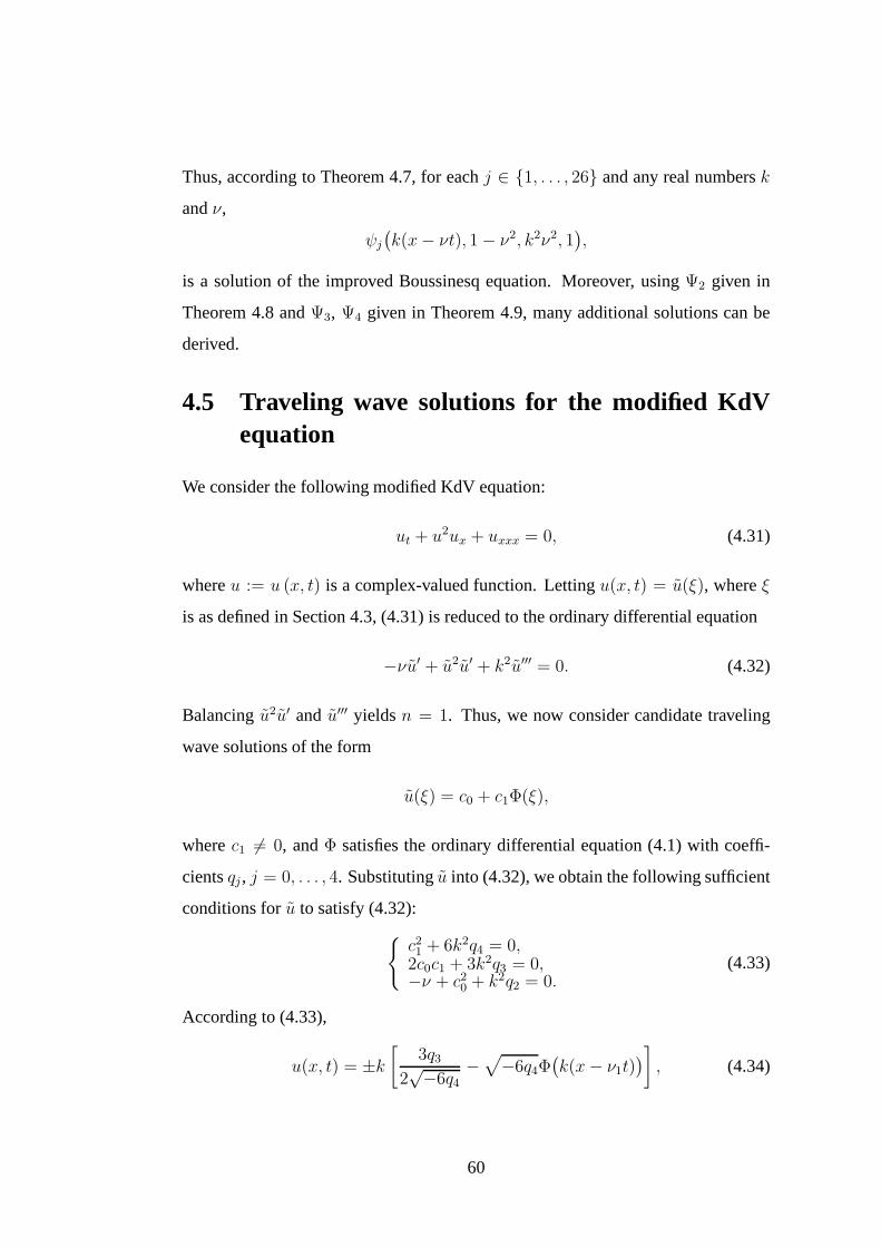
Thus, according to Theorem 4.7, for eachj ∈ {1, . . . , 26} and any real numbersk
andν,
ψj(k(x− νt), 1 − ν2, k2ν2, 1
),
is a solution of the improved Boussinesq equation. Moreover, usingΨ2 given in
Theorem 4.8 andΨ3, Ψ4 given in Theorem 4.9, many additional solutions can be
derived.
4.5 Traveling wave solutions for the modified KdVequation
We consider the following modified KdV equation:
ut + u2ux + uxxx = 0, (4.31)
whereu := u (x, t) is a complex-valued function. Lettingu(x, t) = u(ξ), whereξ
is as defined in Section 4.3, (4.31) is reduced to the ordinarydifferential equation
−νu′ + u2u′ + k2u′′′ = 0. (4.32)
Balancingu2u′ and u′′′ yieldsn = 1. Thus, we now consider candidate traveling
wave solutions of the form
u(ξ) = c0 + c1Φ(ξ),
wherec1 6= 0, andΦ satisfies the ordinary differential equation (4.1) with coeffi-
cientsqj , j = 0, . . . , 4. Substitutingu into (4.32), we obtain the following sufficient
conditions foru to satisfy (4.32):{c21 + 6k2q4 = 0,2c0c1 + 3k2q3 = 0,−ν + c20 + k2q2 = 0.
(4.33)
According to (4.33),
u(x, t) = ±k[
3q32√−6q4
−√
−6q4Φ(k(x− ν1t)
)], (4.34)
60
is a solution of (4.31) in whichν1 = k2(q2 − 3q23
8q4
)andk is an arbitrary constant.
Now, if q1 = q3 = 0 andq0 6= 0, then Theorem 4.2 can be applied with (4.34) to
give the following solution form of (4.31):
u(x, t) = ǫ1k√
−6q0
[ǫ2
√q4q0
Φ(k(x− ν2t)
)+
1
Φ(k(x− ν2t)
)], (4.35)
whereǫj = ±1, j = 1, 2, ν2 = k2(q2 − ǫ26q0
√q4q0
)andk is an arbitrary constant.
In addition, ifq4 =q0q23q21
andq0q1 6= 0, then Theorem 4.3 can be applied with (4.34)
to yield another solution form of (4.31):
u(x, t) = ±k(
3q12√−6q0
−√−6q0
[q3q1
Φ(k(x−ν3t)
)+
1
Φ(k(x− ν3t)
)])
, (4.36)
whereν3 = k2(q2 − 6q0q3
q1− 3q21
8q0
)andk is an arbitrary constant.
We can apply Theorem 4.4 with (4.34) to obtain the following class of travel-
ing wave solutions of (4.31):
u1 (x, t) = λ+3ϑk2
λ
e−k(x−(k2+λ2)t) + ϑ+ ϑ2(2λ2+3k2)8λ2 ek(x−(k2+λ2)t)
,
whereλ, ϑ andk are arbitrary parameters such thatλ 6= 0. It is noted that, ifλ,
ϑ andk are all real constants satisfyingλϑk 6= 0, thenu1 describes a single wave
traveling in thex-direction andu1(x, t) → λ, ask(x− (k2 + λ2)t) → ±∞.
We can also apply Theorem 4.5 with (4.36) to obtain another class of solutions
of (4.31):
u2 (x, t) =ǫ1
√−6k
σ − 1
[σ + 1
2− σe−k(x−ν4t) + 1
2λ(σ + 1) + 12ǫ2
√λ2 − 4ϑ(σ − 1) + ϑek(x−ν4t)
e−k(x−ν4t) + λ + ϑek(x−ν4t)
]
−ǫ1
√−6kσ
σ − 1
[e−k(x−ν4t) + λ + ϑek(x−ν4t)
σe−k(x−ν4t) + 12λ(σ + 1) + 1
2ǫ2√
λ2 − 4ϑ(σ − 1) + ϑek(x−ν4t)
],
whereǫj = ±1, j = 1, 2, ν4 = k2(σ2+10σ+1)2(σ−1)2
, andλ, ϑ andσ are arbitrary constants
such thatσ 6= 1. Note thatu1 is the same as solution (18) in [45], obtained using
the Exp-function method. However,u2 is a new solution.
We also can obtain Jacobi elliptic solutions to the modified KdV equation
(4.31) by combining Theorem 4.1 with (4.34)-(4.36).
61

1. Forl ∈ {1, . . . , 4}, j ∈ {1, . . . , 12} andγ arbitrary, (4.34) withΦ = ϕj,l(·, γ)andqn = pj,n(γ), n = 0, . . . , 4, is a solution of (4.31).
2. For l ∈ {1, . . . , 4} andj ∈ {1, 2, 3, 4, 5, 6, 9, 11}, (4.35) withΦ = ϕj,l(·, 0)
andqn = pj,n(0), n = 0, . . . , 4, is a solution of (4.31).
3. For l ∈ {1, . . . , 4} andj ∈ {10, 12}, (4.36) withΦ = ϕj,l(·, 0) andqn =
pj,n(0), n = 0, . . . , 4, is a solution of (4.31).
Thus, we can obtain many Jacobi elliptic solutions of (4.31). To keep the details to
minimum, we will not list them all here. Instead, we just select some of them to
compare our results with those reported in [89, 117]. Note that our method can also
be applied to the modified KdV equation considered in [89, 117].
Let γ be such thatγ 6= ±1 andγ 6= ±m. Choosingqj = p2,j(γ), j = 0, . . . , 4,
from (4.34), it follows that
u3(x, t)= k
{3γ(1 + m2 − 2γ2)√−6(m2 − γ2)(1 − γ2)
−√−6(m2 − γ2)(1 − γ2) sn[k(x − ν5t)]
γ sn[k(x − ν5t)] + 1
},
u4(x, t)= k
{3γ(1 + m2 − 2γ2)√−6(m2 − γ2)(1 − γ2)
−√−6(m2 − γ2)(1 − γ2)
γ + m sn[k(x − ν5t)]
},
u5(x, t)= k
{3γ(1 + m2 − 2γ2)√−6(m2 − γ2)(1 − γ2)
−√−6(m2 − γ2)(1 − γ2) dn[k(x − ν5t)]
γ dn[k(x − ν5t)] + m cn[k(x − ν5t)]
},
u6(x, t)= k
{3γ(1 + m2 − 2γ2)√−6(m2 − γ2)(1 − γ2)
−√−6(m2 − γ2)(1 − γ2) cn[k(x − ν5t)]
γ cn[k(x − ν5t)] + dn[k(x − ν5t)]
},
are solutions of (4.31) in whichν5 = k2[6γ2 − 1 −m2 − 3γ2(1+m2−2γ2)2
2(m2−γ2)(1−γ2)
]andk
is an arbitrary constant. Ifγ is any real number such thatm < |γ| < 1, thenuj,
j = 3, . . . , 6, are real and bounded. Moreover, ifγ = 0, then according to (4.35),
we can obtain the following two unbounded solutions:
u7(x, t)=√−6k
{±m sn[k(x − ν6t)] +
1
sn[k(x − ν6t)]
},
u8(x, t)=√−6k
{± dn[k(x − ν6t)]
cn[k(x − ν6t)]+
m cn[k(x − ν6t)]
dn[k(x − ν6t)]
},
whereν6 = −k2(1 ± 6m+m2) andk is an arbitrary constant.
62
Similarly, if qj = p3,j(γ), j = 0, . . . , 4, whereγ is an arbitrary constant such
thatγ 6= ±1 andγ 6= ±i m√1−m2 , then we get solutions of (4.31) as follows:
u9(x, t) =k{ 3γ(1 − 2m2 − 2γ2 + 2γ2m2)√
−6(γ2m2 − m2 − γ2)(1 − γ2)
−√−6(γ2m2 − m2 − γ2)(1 − γ2) cn[k(x − ν7t)]
γ cn[k(x − ν7t)] + 1
},
u10(x, t) =k{ 3γ(1 − 2m2 − 2γ2 + 2γ2m2)√
−6(γ2m2 − m2 − γ2)(1 − γ2)
−√
6(γ2m2 − m2 − γ2)(1 − γ2)(1 − m2)
γ√
m2 − 1 + m cn[k(x − ν7t)]
},
u11(x, t) =k{ 3γ(1 − 2m2 − 2γ2 + 2γ2m2)√
−6(γ2m2 − m2 − γ2)(1 − γ2)
−p
−6(γ2m2 −m2 − γ2)(1 − γ2) dn[k(x− ν7t)]
γ dn[k(x− ν7t)] + im sn[k(x− ν7t)]
o
,
u12(x, t) =k{ 3γ(1 − 2m2 − 2γ2 + 2γ2m2)√
−6(γ2m2 − m2 − γ2)(1 − γ2)
−√−6(γ2m2 − m2 − γ2)(1 − γ2)(1 − m2) sn[k(x − ν7t)]
γ√
1 − m2 sn[k(x − ν7t)] + dn[k(x − ν7t)]
},
whereν7 = k2[2m2 − 6γ2m2 + 6γ2 − 1 − 3γ2(1−2m2−2γ2+2γ2m2)2
2(m2γ2−m2−γ2)(1−γ2)
]andk is an ar-
bitrary constant. Moreover, ifγ = 0, then we have the unbounded solutions
u13(x, t)= k√
6(m2 − 1)
{± m√
m2 − 1cn[k(x − ν8t)] +
1
cn[k(x − ν8t)]
},
u14(x, t)= k√
6(1 − m2)
{∓ 1√
m2 − 1
dn[k(x − ν8t)]
sn[k(x − ν8t)]+ m
sn[k(x − ν8t)]
dn[k(x − ν8t)]
},
whereν8 = k2(2m2 − 1 ± 6m√m2 − 1) andk is an arbitrary constant.
If qj = p6,j(γ), j = 0, . . . , 4, whereγ is an arbitrary constant such that
63
m2γ4 +m2 +4γ2 −2m2γ2 6= 0, then we can obtain another four solutions of (4.31)
u15(x, t) =k{ 3γ(γ2m2 − m2 + 2)√
6(γ4m2 + m2 + 4γ2 − 2γ2m2)
−√
6(γ4m2 + m2 + 4γ2 − 2γ2m2)
2γ + i2 sn[k(x − ν9t)] + 2 cn[k(x − ν9t)]
},
u16(x, t) =k{ 3γ(γ2m2 − m2 + 2)√
6(γ4m2 + m2 + 4γ2 − 2γ2m2)
−√
6(γ4m2 + m2 + 4γ2 − 2γ2m2) dn[k(x − ν9t)]
2γ dn[k(x − ν9t)] + i2 cn[k(x − ν9t)] + 2√
1 − m2 sn[k(x − ν9t)]
},
u17(x, t) =k{ 3γ(γ2m2 − m2 + 2)√
6(γ4m2 + m2 + 4γ2 − 2γ2m2)
−√
6(γ4m2 + m2 + 4γ2 − 2γ2m2)m sn[k(x − ν9t)]
2γm sn[k(x − ν9t)] + i2 + i2 dn[k(x − ν9t)]
},
u18(x, t) =k{ 3γ(γ2m2 − m2 + 2)√
6(γ4m2 + m2 + 4γ2 − 2γ2m2)
−√
6(γ4m2 + m2 + 4γ2 − 2γ2m2)im cn[k(x − ν9t)]
i2γm cn[k(x − ν9t)] + 2 dn[k(x − ν9t)] + 2√
1 − m2
},
whereν9 = k2[m2−3γ2m2−2
2+ 3γ2(γ2m2−m2+2)2
2(m2γ4+m2+4γ2−2m2γ2)
]and k is an arbitrary con-
stant. Furthermore, choosingγ = 0 yields that, for anyk,
u19(x, t)=√−6km sn[kx + k3(m2 + 1)t],
u20(x, t)=√−6k
1
sn[kx + k3(m2 + 1)t],
u21(x, t)=√−6km
cn[kx + k3(m2 + 1)t]
dn[kx + k3(m2 + 1)t],
u22(x, t)=√−6k
dn[kx + k3(m2 + 1)t]
cn[kx + k3(m2 + 1)t],
u23(x, t)=√
6km cn[kx − k3(2m2 − 1)t],
u24(x, t)= k√
6(m2 − 1)1
cn[kx − k3(2m2 − 1)t],
u25(x, t)= k√−6
dn[kx − k3(2m2 − 1)t]
sn[kx − k3(2m2 − 1)t],
u26(x, t)= km√
6(1 − m2)sn[kx − k3(2m2 − 1)t]
dn[kx − k3(2m2 − 1)t],
are solutions of (4.31).
Remark 4.8. It follows from Remark 4.1 thatuj, j = 3, . . . , 26, still satisfy
(4.31) even if cn(·), sn(·) and dn(·) are replaced, respectively, by±cn(·), ±sn(·)and±dn(·).
64
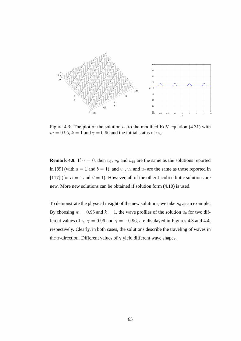
−20
−10
0
10
20
0
5
10100
5
x
t
u
−20 −15 −10 −5 0 5 10 15 2020−20
−15
−10
−5
0
5
10
15
2020
x
u
Figure 4.3: The plot of the solutionu6 to the modified KdV equation (4.31) withm = 0.95, k = 1 andγ = 0.96 and the initial status ofu6.
Remark 4.9. If γ = 0, thenu3, u9 andu15 are the same as the solutions reported
in [89] (with a = 1 andb = 1), andu3, u4 andu7 are the same as those reported in
[117] (for α = 1 andβ = 1). However, all of the other Jacobi elliptic solutions are
new. More new solutions can be obtained if solution form (4.10) is used.
To demonstrate the physical insight of the new solutions, wetakeu6 as an example.
By choosingm = 0.95 andk = 1, the wave profiles of the solutionu6 for two dif-
ferent values ofγ, γ = 0.96 andγ = −0.96, are displayed in Figures 4.3 and 4.4,
respectively. Clearly, in both cases, the solutions describe the traveling of waves in
thex-direction. Different values ofγ yield different wave shapes.
65
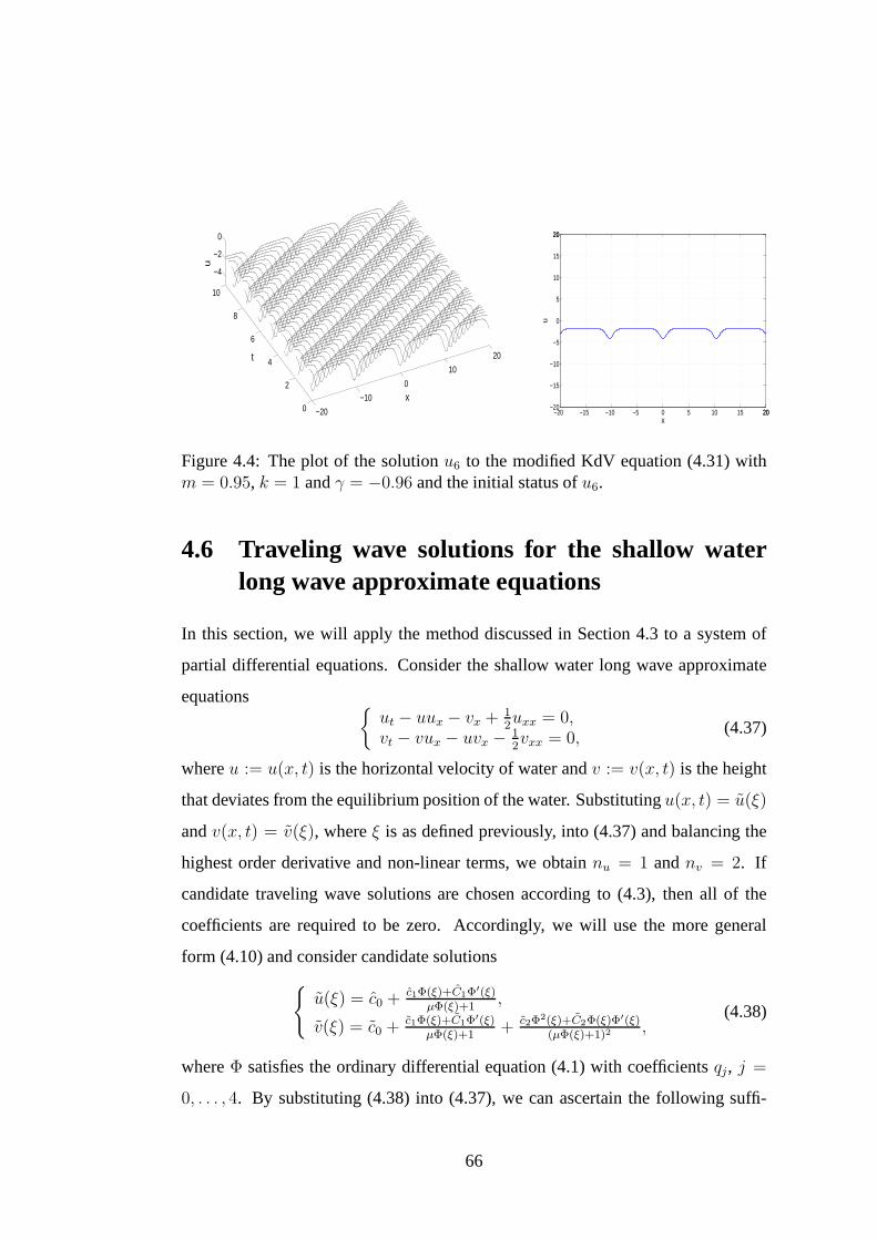
−20
−10
0
10
20
0
2
4
6
8
10
−4
−2
0
x
t
u
−20 −15 −10 −5 0 5 10 15 2020−20
−15
−10
−5
0
5
10
15
2020
x
u
Figure 4.4: The plot of the solutionu6 to the modified KdV equation (4.31) withm = 0.95, k = 1 andγ = −0.96 and the initial status ofu6.
4.6 Traveling wave solutions for the shallow waterlong wave approximate equations
In this section, we will apply the method discussed in Section 4.3 to a system of
partial differential equations. Consider the shallow water long wave approximate
equations {ut − uux − vx + 1
2uxx = 0,
vt − vux − uvx − 12vxx = 0,
(4.37)
whereu := u(x, t) is the horizontal velocity of water andv := v(x, t) is the height
that deviates from the equilibrium position of the water. Substitutingu(x, t) = u(ξ)
andv(x, t) = v(ξ), whereξ is as defined previously, into (4.37) and balancing the
highest order derivative and non-linear terms, we obtainnu = 1 andnv = 2. If
candidate traveling wave solutions are chosen according to(4.3), then all of the
coefficients are required to be zero. Accordingly, we will use the more general
form (4.10) and consider candidate solutions
{u(ξ) = c0 + c1Φ(ξ)+C1Φ′(ξ)
µΦ(ξ)+1,
v(ξ) = c0 + c1Φ(ξ)+C1Φ′(ξ)µΦ(ξ)+1
+ c2Φ2(ξ)+C2Φ(ξ)Φ′(ξ)(µΦ(ξ)+1)2
,(4.38)
whereΦ satisfies the ordinary differential equation (4.1) with coefficients qj, j =
0, . . . , 4. By substituting (4.38) into (4.37), we can ascertain the following suffi-
66
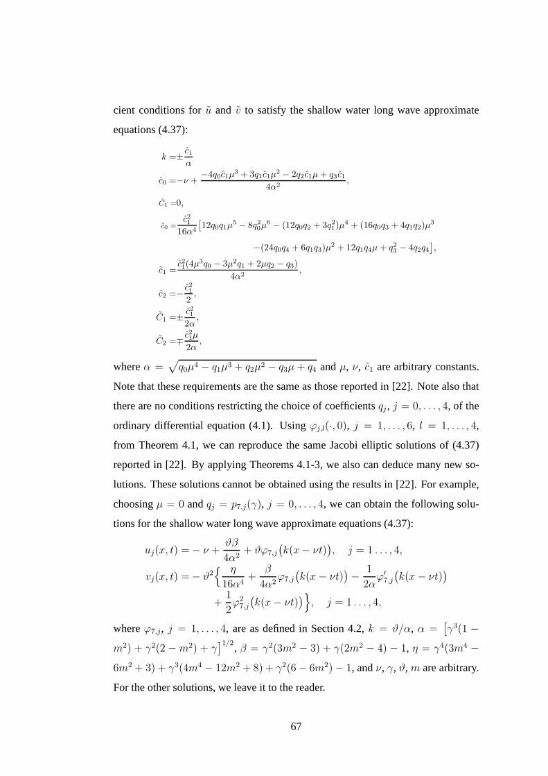
cient conditions foru and v to satisfy the shallow water long wave approximate
equations (4.37):
k =± c1
α
c0 =−ν +−4q0c1µ
3 + 3q1c1µ2 − 2q2c1µ + q3c1
4α2,
C1 =0,
c0 =c21
16α4
[12q0q1µ
5 − 8q20µ
6 − (12q0q2 + 3q21)µ
4 + (16q0q3 + 4q1q2)µ3
−(24q0q4 + 6q1q3)µ2 + 12q1q4µ + q2
3 − 4q2q4
],
c1 =c21(4µ3q0 − 3µ2q1 + 2µq2 − q3)
4α2,
c2 =− c21
2,
C1 =± c21
2α,
C2 =∓ c21µ
2α,
whereα =√q0µ4 − q1µ3 + q2µ2 − q3µ+ q4 andµ, ν, c1 are arbitrary constants.
Note that these requirements are the same as those reported in [22]. Note also that
there are no conditions restricting the choice of coefficients qj , j = 0, . . . , 4, of the
ordinary differential equation (4.1). Usingϕj,l(·, 0), j = 1, . . . , 6, l = 1, . . . , 4,
from Theorem 4.1, we can reproduce the same Jacobi elliptic solutions of (4.37)
reported in [22]. By applying Theorems 4.1-3, we also can deduce many new so-
lutions. These solutions cannot be obtained using the results in [22]. For example,
choosingµ = 0 andqj = p7,j(γ), j = 0, . . . , 4, we can obtain the following solu-
tions for the shallow water long wave approximate equations(4.37):
uj(x, t) = − ν +ϑβ
4α2+ ϑϕ7,j
(k(x− νt)
), j = 1 . . . , 4,
vj(x, t) = − ϑ2{ η
16α4+
β
4α2ϕ7,j
(k(x− νt)
)− 1
2αϕ′
7,j
(k(x− νt)
)
+1
2ϕ2
7,j
(k(x− νt)
)}, j = 1 . . . , 4,
whereϕ7,j, j = 1, . . . , 4, are as defined in Section 4.2,k = ϑ/α, α =[γ3(1 −
m2) + γ2(2 −m2) + γ]1/2
, β = γ2(3m2 − 3) + γ(2m2 − 4) − 1, η = γ4(3m4 −6m2 + 3) + γ3(4m4 − 12m2 + 8) + γ2(6 − 6m2) − 1, andν, γ, ϑ,m are arbitrary.
For the other solutions, we leave it to the reader.
67

−20
−10
0
10
20
0
2
4
6
8
101.5
22.5
x
t
u
−20 −10 0 10 2020−4
−2
0
2
44
x
u
Figure 4.5: The plot of the solutionu1 of the shallow water long wave approximateequations (4.37) withm = 0.99, ν = −2 andϑ = γ = 1 and the initial status ofu1.
To show the physical insight of these solutions, we take the solution (u1, v1)
as an example. Figures 4.5 and 4.6 display the graphs ofu1 andv1 with m = 0.99,
ν = −2 andϑ = γ = 1. Clearly, the solution describes the propagation of waves
with horizontal velocityu1 along the negativex-direction.
4.7 Concluding remarks
In this chapter, we have presented a generalized expansion method for generating
traveling wave solutions of non-linear partial differential equations. This method
has been successfully applied to the Boussinesq equation, the modified KdV equa-
tion and the shallow water long wave approximate equations,and many new results
have been obtained. For each equation investigated, we are able to replicate solu-
tions previously derived in the literature, and discover many new ones. Extensions
to two and three dimensional partial differential equations are possible. Other non-
linear partial differential equations can be tackled if an appropriate transformation
can be found. For example, in [45], the transformationu = ln v was applied to the
Dodd-Bullough-Mikhailov equation to yield a non-linear partial differential equa-
tion involving powers ofv and its derivatives.
68
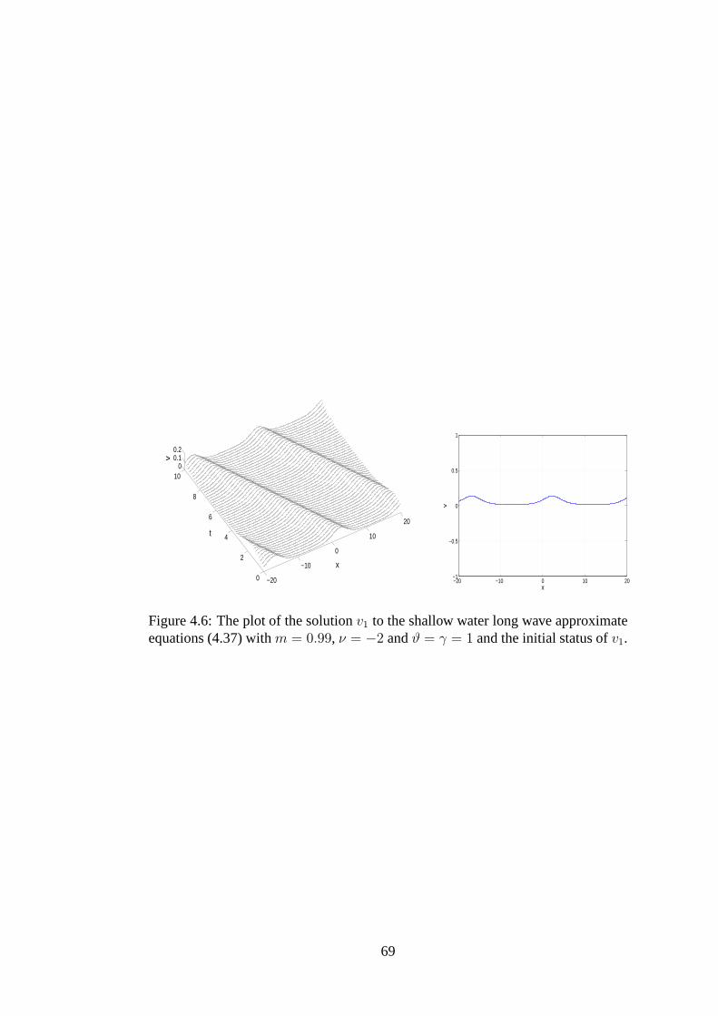
−20
−10
0
10
20
0
2
4
6
8
100
0.10.2
x
t
v
−20 −10 0 10 20−1
−0.5
0
0.5
1
x
v
Figure 4.6: The plot of the solutionv1 to the shallow water long wave approximateequations (4.37) withm = 0.99, ν = −2 andϑ = γ = 1 and the initial status ofv1.
69
Chapter 5
Linear B-spline finite elementmethod for the improved Boussinesqequation
5.1 Introductory remarks
The improved Boussinesq equation (1.3) has been studied extensively over the past
two decades (see [1, 18, 20, 33, 47, 50]). Iskandar and Jain [50] were the first
to investigate the improved Boussinesq equation (1.3) numerically. Applying a lin-
earization technique and finite difference approximations, Iskandar and Jain derived
a three-level iterative scheme with second order local truncation error. The scheme
was used to investigate head-on collisions between solitary waves. Later, Zoheiry
[33] developed an improved scheme with a Crank-Nicolson modification. For this
scheme, each time step is accompanied by an iterative process that ensures the ac-
curacy requirements are satisfied. Hence, whilst accuracy is maintained, efficiency
is compromised.
In [47], Adomian’s decomposition method was applied to the Cauchy problem
for the improved Boussinesq equation (1.3). Using this method, the solution is
expressed as a convergent series, and an approximation is obtained by truncating
the series after a sufficient number of terms. However, the computation of each
term in this series is cumbersome, requiring the integration and differentiation of
several complex expressions. The symbolic manipulation package Maple was used
70
and numerical results were calculated and compared with theanalytical solution, but
only for a very small value oft. It remains to be seen how this method performs for
large values oft. In fact, in order to maintain accuracy ast increases, it is expected
that a large number of more complicated terms will need to be calculated. In [1], the
Adomian decomposition-Pade technique has been presentedand it has been shown
that this technique gives the approximate solution with faster convergence rate and
higher accuracy than using Adomian’s decomposition methodalone. However, the
disadvantage of Adomian’s decomposition method still remains, that is, the error
increases rapidly ast increases.
In [18], Bratsos considered the improved Boussinesq equation (1.3) with bound-
ary conditions imposed on the first spatial derivative. Finite difference approxima-
tions were used to reduce the improved Boussinesq equation (1.3) to a system of
ordinary differential equations. Using a Pade approximation, a three level implicit
time-step scheme was developed. Relevant stability boundswere also derived. In
addition, Bratsos has employed an implicit finite-difference method associated with
a predictor-corrector scheme to solve the initial boundaryvalue problem governed
by the improved Boussinesq equation (1.3) (see [20]).
In this chapter, we develop a Galerkin-based finite element method for a class
of initial boundary value problems governed by the improvedBoussinesq equa-
tion (1.3). The spatial axis is partitioned into a set of finite elements and the solution
is expressed in terms of the linear B-spline basis functions. On this basis, a system
involving only ordinary derivatives is obtained. Then, thestructure of the system co-
efficient matrices is exploited to transform the problem into an explicit initial value
problem. Accordingly, many standard numerical integration algorithms are appli-
cable. In this manner, an approximate solution to the problem can be generated.
In contrast to existing methods, this method is simple to implement and capable
of handling the non-linearity in the governing equation. Wepresent the results of
four numerical experiments to validate the method and demonstrate its capability in
simulating complex wave phenomena.
71
5.2 Problem statement
Consider the initial boundary value problem consisting of the improved Boussinesq
equation
utt = uxx + uxxtt +(u2)xx, x ∈ (a, b), t > 0, (5.1)
the initial conditions
u(x, 0) = u0(x), ut(x, 0) = u1(x), for all x ∈ (a, b), (5.2)
and the boundary conditions
u(a, t) = 0, u(b, t) = 0, for all t ∈ (0,∞), (5.3)
whereu0, u1 : (a, b) → R are given functions.
For any fixedt, we multiply (5.1) by a test functionv ∈ H10 (a, b) = {w ∈
L2(a, b) : wx ∈ L2(a, b), w(a) = w(b) = 0}, integrate the product over[a, b] using
integration by parts, and then apply the boundary conditions (5.3) to yield∫ b
a
(uttv + uxvx + uxttvx + (u2)xvx
)dx = 0, (5.4)
where the function arguments are suppressed for clarity. Equation (5.4) is required
to hold for all admissible test functions. On this basis, we define the following vari-
ational problem.
Problem 5.1.Find au ∈ H10 (a, b) such that (5.2) is satisfied and, for eacht > 0,
(utt, v) + (ux, vx) + (uxtt, vx) +((u2)x, vx
)= 0, for all v ∈ H1
0 (a, b), (5.5)
where
(u, v) =
∫ b
a
u(x)v(x)dx.
5.3 Numerical method
We partition thex-axis inton finite elements by choosing a set of evenly-spaced
knots{xi}ni=0 such thata = x0 < x1 < · · · < xn−1 < xn = b andxi+1 − xi = h,
72
i = 0, . . . , n− 1. Consider an approximate solution of Problem 5.1 of the form:
Un(x, t) =
n∑
i=0
ui(t)φi(x), (5.6)
where
φi(x) =
x− xi−1
xi − xi−1, x ∈ [xi−1, xi],
xi+1 − x
xi+1 − xi, x ∈ [xi, xi+1],
0, elsewhere.
According to (5.6),ui(t) = Un(xi, t), i = 0, . . . , n.
Applying the boundary conditions (5.3) givesu0(t) = 0 andun(t) = 0 for all
t ∈ (0,∞). Hence, (5.6) can be simplified to
Un(x, t) =n−1∑
i=1
ui(t)φi(x). (5.7)
We then follow the standard Galerkin approach and choose test functionsv = φi,
i = 1, . . . , n − 1. On this basis, (5.5) must hold withv = φi, i = 1, . . . , n − 1.
Substituting (5.7) into (5.5) gives
n−1∑
j=1
((φi, φj) uj +
(φ′i, φ
′j
)uj +
(φ′i, φ
′j
)uj + 2
n−1∑
k=1
(φ′iφ
′k, φj) ukuj
)= 0 (5.8)
for eachi = 1, . . . , n− 1, where′ and denote differentiation with respect tox and
t, respectively.
In matrix notation, the system of equations (5.8) can be written as
(A+B)U(t) +BU(t) + C(U(t)
)U(t) = 0, (5.9)
where0 ∈ Rn−1 is a zero vector andU(t) =
[u1(t), u2(t), . . . , un−1(t)
]T. The
(n− 1) × (n− 1) matricesA, B andC(U(t)
)are given as follows:
A =[(φi, φj)
]=h
6
4 1 0 · · · 01 4 1 · · · 00 1 4 · · · 0...
......
. . ....
0 0 0 · · · 4
,
B =[(φ′
i, φ′j)]
=1
h
2 −1 0 · · · 0−1 2 −1 · · · 00 −1 2 · · · 0...
......
. . ....
0 0 0 · · · 2
,
73
and
C(U(t)
)=
[2n−1∑k=1
(φ′iφ
′k, φj)uk
]
=1
h
2u1 − u2 u1 − u2 0 · · · 0u2 − u1 −u1 + 2u2 − u3 u2 − u3 · · · 0
0 u3 − u2 −u2 + 2u3 − u4 · · · 0...
......
. . ....
0 0 0 · · · −un−2 + 2un−1
.
Note thatC is a time dependent matrix, whilstA andB are constant. By virtue of
the structure ofA andB, we have the following theorem.
Theorem 5.1. The matrixA+B is invertible.
Proof. Let y ∈ Rn−1 be a non-zero vector and definew(x) =
n−1∑i=1
yiφi(x).
Then we have
yTBy =
n−1∑
i=1
n−1∑
j=1
yibijyj
=n−1∑
i=1
n−1∑
j=1
yi
(∫ b
a
φ′i(x)φ
′j(x)dx
)yj
=
∫ b
a
n−1∑
i=1
n−1∑
j=1
yiφ′i(x)φ
′j(x)yjdx
=
∫ b
a
(n−1∑
i=1
yiφ′i(x)
)2
dx
=
∫ b
a
(w′(x))2dx
≥ 0.
Sincew′ is piecewise continuous, equality holds if, and only if,w′(x) = 0 for all
x ∈ [a, b]. Now, sincew(a) = 0, w′(x) = 0 for all x ∈ [a, b] if, and only if,w ≡ 0.
This, in turn, requiresy = 0, which contradicts the assumption thaty is non-zero.
Hence,yTBy > 0 for all non-zeroy and soB is positive definite. In a similar
manner, one can ascertain the positive definiteness ofA. Since bothA andB are
74
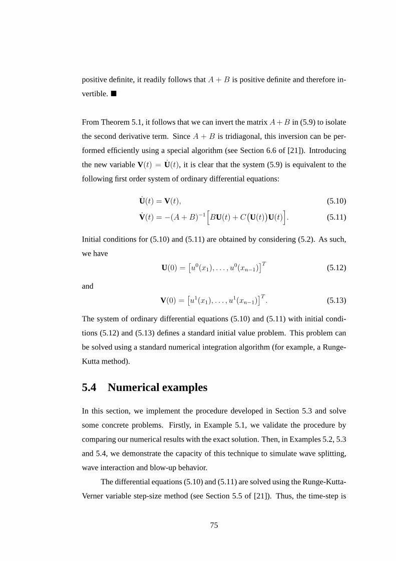
positive definite, it readily follows thatA + B is positive definite and therefore in-
vertible.�
From Theorem 5.1, it follows that we can invert the matrixA+B in (5.9) to isolate
the second derivative term. SinceA + B is tridiagonal, this inversion can be per-
formed efficiently using a special algorithm (see Section 6.6 of [21]). Introducing
the new variableV(t) = U(t), it is clear that the system (5.9) is equivalent to the
following first order system of ordinary differential equations:
U(t) = V(t), (5.10)
V(t) = −(A +B)−1[BU(t) + C
(U(t)
)U(t)
]. (5.11)
Initial conditions for (5.10) and (5.11) are obtained by considering (5.2). As such,
we have
U(0) =[u0(x1), . . . , u
0(xn−1)]T
(5.12)
and
V(0) =[u1(x1), . . . , u
1(xn−1)]T. (5.13)
The system of ordinary differential equations (5.10) and (5.11) with initial condi-
tions (5.12) and (5.13) defines a standard initial value problem. This problem can
be solved using a standard numerical integration algorithm(for example, a Runge-
Kutta method).
5.4 Numerical examples
In this section, we implement the procedure developed in Section 5.3 and solve
some concrete problems. Firstly, in Example 5.1, we validate the procedure by
comparing our numerical results with the exact solution. Then, in Examples 5.2, 5.3
and 5.4, we demonstrate the capacity of this technique to simulate wave splitting,
wave interaction and blow-up behavior.
The differential equations (5.10) and (5.11) are solved using the Runge-Kutta-
Verner variable step-size method (see Section 5.5 of [21]).Thus, the time-step is
75
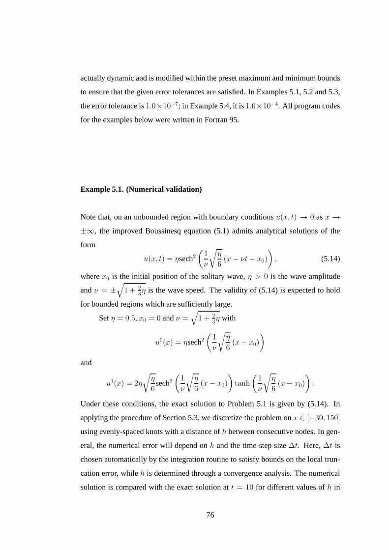
actually dynamic and is modified within the preset maximum and minimum bounds
to ensure that the given error tolerances are satisfied. In Examples 5.1, 5.2 and 5.3,
the error tolerance is1.0×10−7; in Example 5.4, it is1.0×10−4. All program codes
for the examples below were written in Fortran 95.
Example 5.1. (Numerical validation)
Note that, on an unbounded region with boundary conditionsu(x, t) → 0 asx →±∞, the improved Boussinesq equation (5.1) admits analyticalsolutions of the
form
u(x, t) = ηsech2(
1
ν
√η
6(x− νt− x0)
), (5.14)
wherex0 is the initial position of the solitary wave,η > 0 is the wave amplitude
andν = ±√
1 + 23η is the wave speed. The validity of (5.14) is expected to hold
for bounded regions which are sufficiently large.
Setη = 0.5, x0 = 0 andν =√
1 + 23η with
u0(x) = ηsech2(
1
ν
√η
6(x− x0)
)
and
u1(x) = 2η
√η
6sech2
(1
ν
√η
6(x− x0)
)tanh
(1
ν
√η
6(x− x0)
).
Under these conditions, the exact solution to Problem 5.1 isgiven by (5.14). In
applying the procedure of Section 5.3, we discretize the problem onx ∈ [−30, 150]
using evenly-spaced knots with a distance ofh between consecutive nodes. In gen-
eral, the numerical error will depend onh and the time-step size∆t. Here,∆t is
chosen automatically by the integration routine to satisfybounds on the local trun-
cation error, whileh is determined through a convergence analysis. The numerical
solution is compared with the exact solution att = 10 for different values ofh in
76
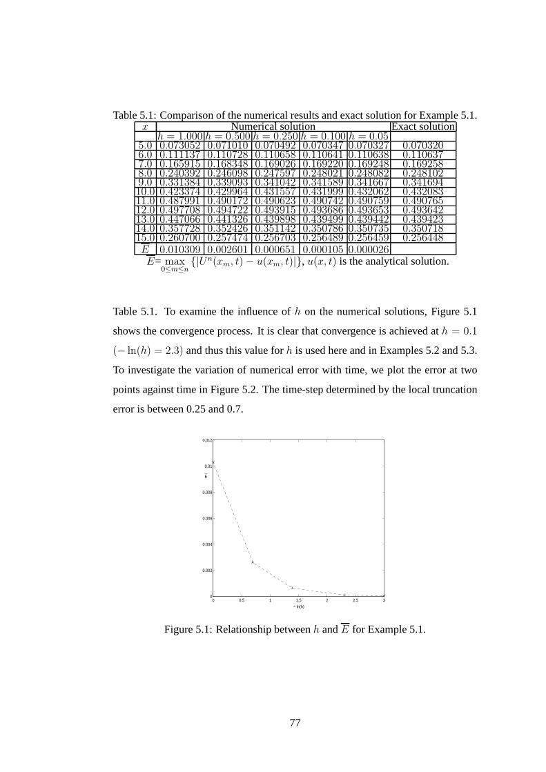
Table 5.1: Comparison of the numerical results and exact solution for Example 5.1.x Numerical solution Exact solution
h = 1.000 h = 0.500 h = 0.250 h = 0.100 h = 0.055.0 0.073052 0.071010 0.070492 0.070347 0.070327 0.0703206.0 0.111137 0.110728 0.110658 0.110641 0.110638 0.1106377.0 0.165915 0.168348 0.169026 0.169220 0.169248 0.1692588.0 0.240392 0.246098 0.247597 0.248021 0.248082 0.2481029.0 0.331384 0.339093 0.341042 0.341589 0.341667 0.34169410.0 0.423374 0.429964 0.431557 0.431999 0.432062 0.43208311.0 0.487991 0.490172 0.490623 0.490742 0.490759 0.49076512.0 0.497708 0.494722 0.493915 0.493686 0.493653 0.49364213.0 0.447066 0.441326 0.439898 0.439499 0.439442 0.43942314.0 0.357728 0.352426 0.351142 0.350786 0.350735 0.35071815.0 0.260700 0.257474 0.256703 0.256489 0.256459 0.256448E 0.010309 0.002601 0.000651 0.000105 0.000026E= max
0≤m≤n{|Un(xm, t) − u(xm, t)|}, u(x, t) is the analytical solution.
Table 5.1. To examine the influence ofh on the numerical solutions, Figure 5.1
shows the convergence process. It is clear that convergenceis achieved ath = 0.1
(− ln(h) = 2.3) and thus this value forh is used here and in Examples 5.2 and 5.3.
To investigate the variation of numerical error with time, we plot the error at two
points against time in Figure 5.2. The time-step determinedby the local truncation
error is between 0.25 and 0.7.
0 0.5 1 1.5 2 2.5 30
0.002
0.004
0.006
0.008
0.01
0.012
− ln(h)
E
Figure 5.1: Relationship betweenh andE for Example 5.1.
77
0 10 20 30 40 50 60 70−4
−3
−2
−1
0
1
2
3
4x 10
−4
t
err
or=
nu
me
rica
l so
lutio
n −
exa
ct s
olu
tion
. −−−−−−−−− error at x=10* −−−−−−−−− error at x=50
Figure 5.2: Numerical errors versus time atx = 10 andx = 50 for Example 5.1.
The wave profile of the numerical solution fort ∈ [0, 72] is shown in Figure 5.3.
The results are in good agreement with those presented in [18, 15, 33, 50]. The
average speed of this solitary wave is 1.1542, which is quiteclose to the theoretical
value of√
1 + 23η = 1.154701. We note that our numerical method is much more
efficient than those presented in the references. For example, using our method, an
accuracy ofE = 3.96 × 10⁻⁴ at t = 72 is achieved with0.25 ≤ ∆t ≤ 0.7. In [18],
∆t needs to be in the order of 0.001 to generate results of comparable accuracy.
78
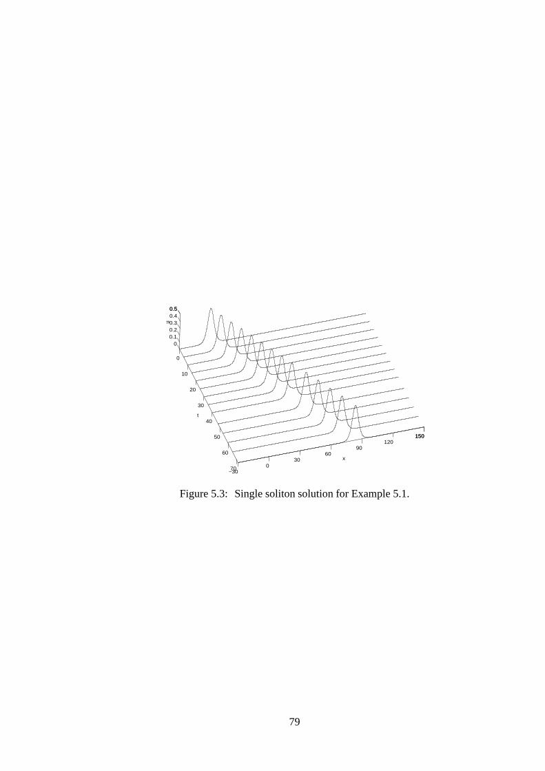
−300
3060
90120
150150
0
10
20
30
40
50
60
70
00.10.20.30.40.50.5
x
t
u
Figure 5.3: Single soliton solution for Example 5.1.
79
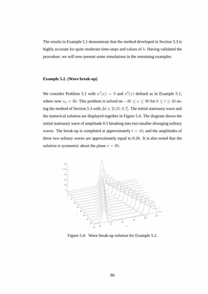
The results in Example 5.1 demonstrate that the method developed in Section 5.3 is
highly accurate for quite moderate time-steps and values ofh. Having validated the
procedure, we will now present some simulations in the remaining examples.
Example 5.2. (Wave break-up)
We consider Problem 5.1 withu1(x) = 0 andu0(x) defined as in Example 5.1,
where nowx0 = 30. This problem is solved on−30 ≤ x ≤ 90 for 0 ≤ t ≤ 40 us-
ing the method of Section 5.3 with∆t ∈ [0.25, 0.7]. The initial stationary wave and
the numerical solution are displayed together in Figure 5.4. The diagram shows the
initial stationary wave of amplitude 0.5 breaking into two smaller diverging solitary
waves. The break-up is completed at approximatelyt = 10, and the amplitudes of
these two solitary waves are approximately equal to 0.26. Itis also noted that the
solution is symmetric about the planex = 30.
−200
2040
6080
0
5
10
15
20
25
30
35
40
0
0.1
0.2
0.3
0.4
0.5
x
t
u
Figure 5.4: Wave break-up solution for Example 5.2.
80
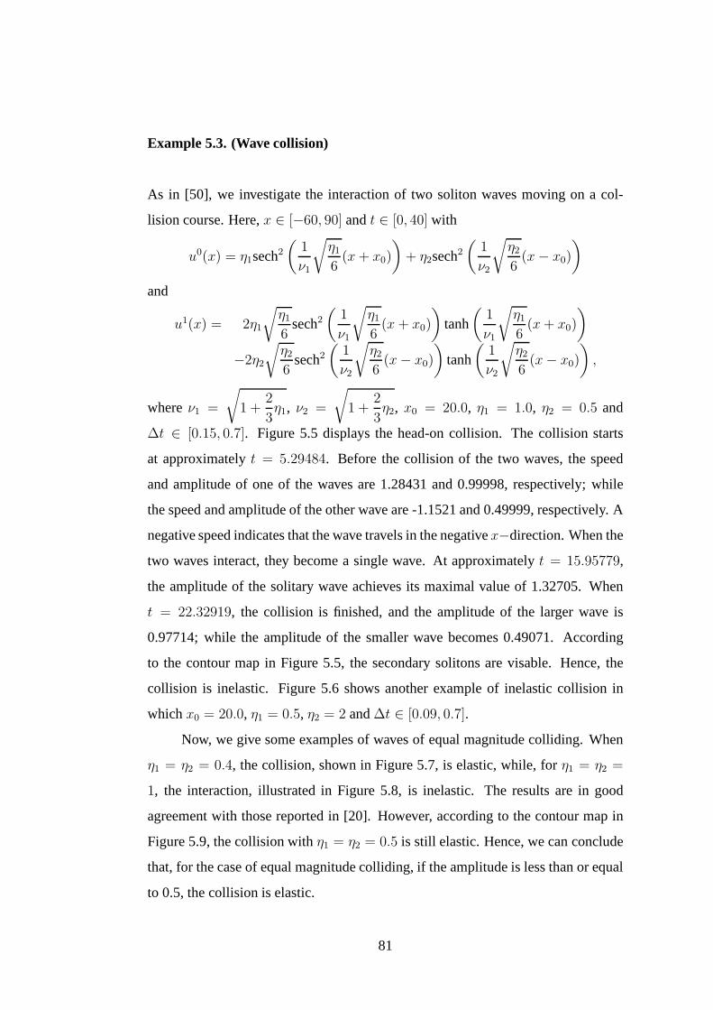
Example 5.3. (Wave collision)
As in [50], we investigate the interaction of two soliton waves moving on a col-
lision course. Here,x ∈ [−60, 90] andt ∈ [0, 40] with
u0(x) = η1sech2(
1
ν1
√η1
6(x+ x0)
)+ η2sech2
(1
ν2
√η2
6(x− x0)
)
and
u1(x) = 2η1
√η1
6sech2
(1
ν1
√η1
6(x+ x0)
)tanh
(1
ν1
√η1
6(x+ x0)
)
−2η2
√η2
6sech2
(1
ν2
√η2
6(x− x0)
)tanh
(1
ν2
√η2
6(x− x0)
),
whereν1 =
√1 +
2
3η1, ν2 =
√1 +
2
3η2, x0 = 20.0, η1 = 1.0, η2 = 0.5 and
∆t ∈ [0.15, 0.7]. Figure 5.5 displays the head-on collision. The collision starts
at approximatelyt = 5.29484. Before the collision of the two waves, the speed
and amplitude of one of the waves are 1.28431 and 0.99998, respectively; while
the speed and amplitude of the other wave are -1.1521 and 0.49999, respectively. A
negative speed indicates that the wave travels in the negativex−direction. When the
two waves interact, they become a single wave. At approximately t = 15.95779,
the amplitude of the solitary wave achieves its maximal value of 1.32705. When
t = 22.32919, the collision is finished, and the amplitude of the larger wave is
0.97714; while the amplitude of the smaller wave becomes 0.49071. According
to the contour map in Figure 5.5, the secondary solitons are visable. Hence, the
collision is inelastic. Figure 5.6 shows another example ofinelastic collision in
whichx0 = 20.0, η1 = 0.5, η2 = 2 and∆t ∈ [0.09, 0.7].
Now, we give some examples of waves of equal magnitude colliding. When
η1 = η2 = 0.4, the collision, shown in Figure 5.7, is elastic, while, forη1 = η2 =
1, the interaction, illustrated in Figure 5.8, is inelastic.The results are in good
agreement with those reported in [20]. However, according to the contour map in
Figure 5.9, the collision withη1 = η2 = 0.5 is still elastic. Hence, we can conclude
that, for the case of equal magnitude colliding, if the amplitude is less than or equal
to 0.5, the collision is elastic.
81

−60−40
−200
2040
60809090
0
10
20
30
40
0
0.5
1
1.5
x
t
u
x
t
−40 −20 0 20 40 60 800
5
10
15
20
25
30
35
40
Figure 5.5: Inelastic collision withη1 = 1.0 andη2 = 0.5 in Example 5.3. Thecontour line on the right illustration starts from 0.01 and the level step is 0.2.
−60 −40 −20 0 20 40 60 80
0
10
20
30
40
00.5
11.5
22.52.5
t
x
u
x
t
−40 −20 0 20 40 60 800
5
10
15
20
25
30
35
Figure 5.6: Inelastic collision withη1 = 0.5 andη2 = 2.0 in Example 5.3. Thecontour line on the right illustration starts from 0.01 and the level step is 0.3.
82
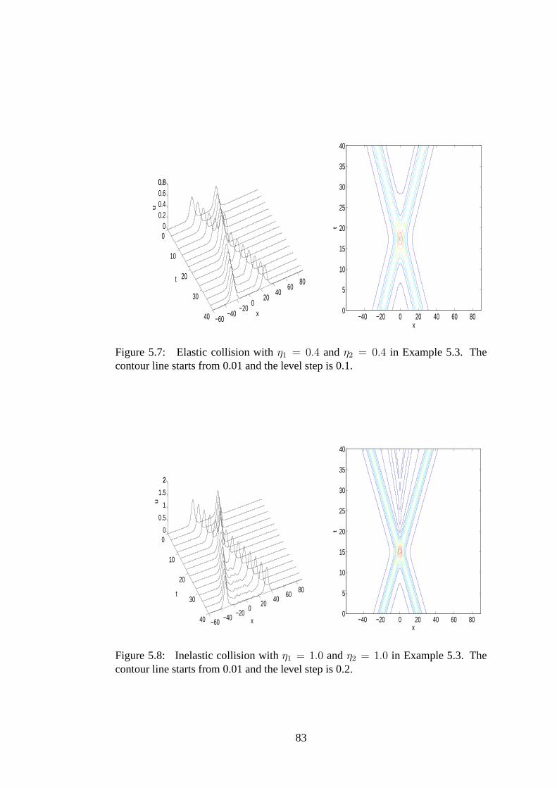
−60−40
−200
2040
6080
0
10
20
30
40
00.20.40.60.80.8
x
t
u
xt
−40 −20 0 20 40 60 800
5
10
15
20
25
30
35
40
Figure 5.7: Elastic collision withη1 = 0.4 andη2 = 0.4 in Example 5.3. Thecontour line starts from 0.01 and the level step is 0.1.
−60−40
−200
2040
6080
0
10
20
30
40
0
0.5
1
1.5
22
x
t
u
x
t
−40 −20 0 20 40 60 800
5
10
15
20
25
30
35
40
Figure 5.8: Inelastic collision withη1 = 1.0 andη2 = 1.0 in Example 5.3. Thecontour line starts from 0.01 and the level step is 0.2.
83
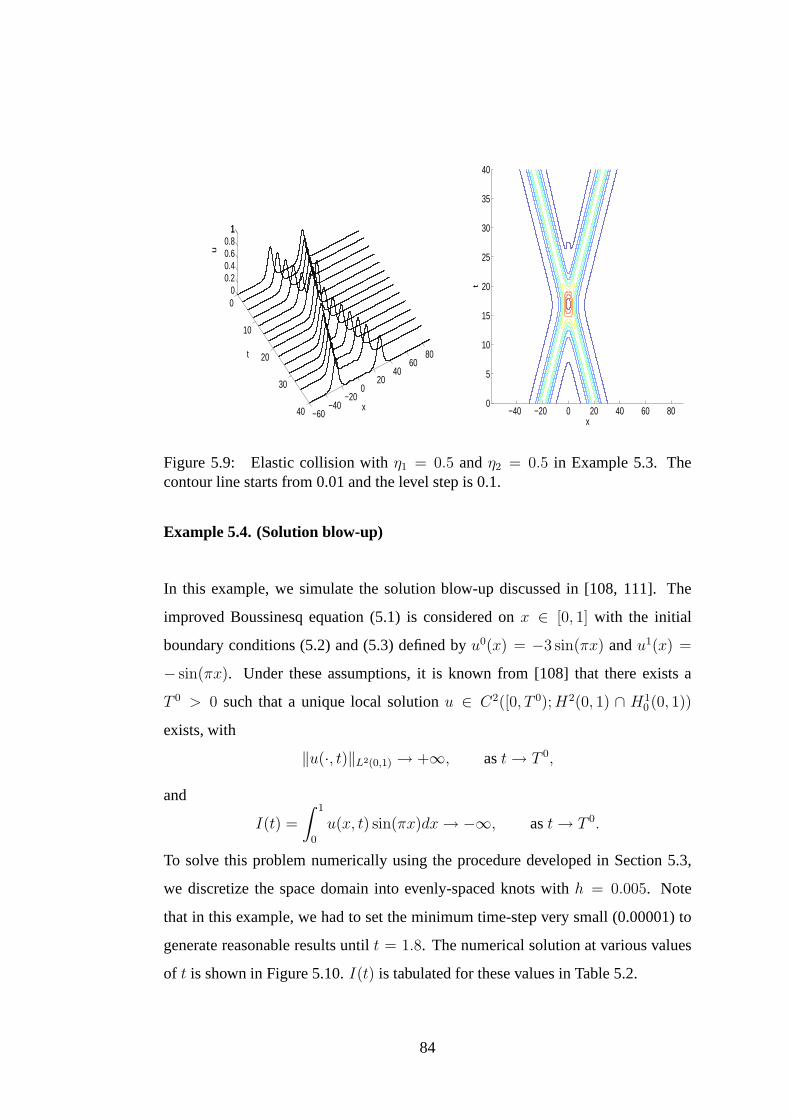
−60−40
−200
2040
6080
0
10
20
30
40
00.20.40.60.8
11
x
t
u
−40 −20 0 20 40 60 800
5
10
15
20
25
30
35
40
x
tFigure 5.9: Elastic collision withη1 = 0.5 andη2 = 0.5 in Example 5.3. Thecontour line starts from 0.01 and the level step is 0.1.
Example 5.4. (Solution blow-up)
In this example, we simulate the solution blow-up discussedin [108, 111]. The
improved Boussinesq equation (5.1) is considered onx ∈ [0, 1] with the initial
boundary conditions (5.2) and (5.3) defined byu0(x) = −3 sin(πx) andu1(x) =
− sin(πx). Under these assumptions, it is known from [108] that there exists a
T 0 > 0 such that a unique local solutionu ∈ C2([0, T 0);H2(0, 1) ∩ H10 (0, 1))
exists, with
‖u(·, t)‖L2(0,1) → +∞, ast→ T 0,
and
I(t) =
∫ 1
0
u(x, t) sin(πx)dx→ −∞, ast→ T 0.
To solve this problem numerically using the procedure developed in Section 5.3,
we discretize the space domain into evenly-spaced knots with h = 0.005. Note
that in this example, we had to set the minimum time-step verysmall (0.00001) to
generate reasonable results untilt = 1.8. The numerical solution at various values
of t is shown in Figure 5.10.I(t) is tabulated for these values in Table 5.2.
84
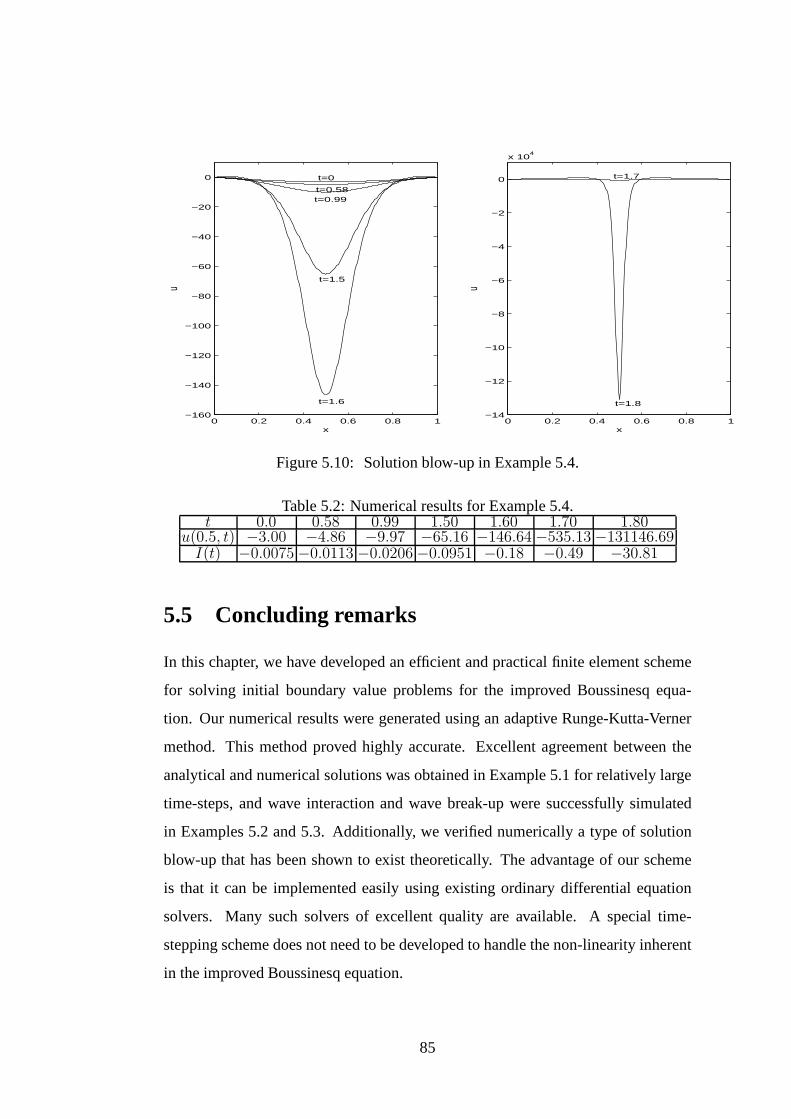
0 0.2 0.4 0.6 0.8 1−160
−140
−120
−100
−80
−60
−40
−20
0
x
u
0 0.2 0.4 0.6 0.8 1−14
−12
−10
−8
−6
−4
−2
0
x 104
x
u
t=0
t=0.58t=0.99
t=1.5
t=1.6
t=1.7
t=1.8
Figure 5.10: Solution blow-up in Example 5.4.
Table 5.2: Numerical results for Example 5.4.t 0.0 0.58 0.99 1.50 1.60 1.70 1.80
u(0.5, t) −3.00 −4.86 −9.97 −65.16 −146.64 −535.13 −131146.69I(t) −0.0075 −0.0113 −0.0206 −0.0951 −0.18 −0.49 −30.81
5.5 Concluding remarks
In this chapter, we have developed an efficient and practicalfinite element scheme
for solving initial boundary value problems for the improved Boussinesq equa-
tion. Our numerical results were generated using an adaptive Runge-Kutta-Verner
method. This method proved highly accurate. Excellent agreement between the
analytical and numerical solutions was obtained in Example5.1 for relatively large
time-steps, and wave interaction and wave break-up were successfully simulated
in Examples 5.2 and 5.3. Additionally, we verified numerically a type of solution
blow-up that has been shown to exist theoretically. The advantage of our scheme
is that it can be implemented easily using existing ordinarydifferential equation
solvers. Many such solvers of excellent quality are available. A special time-
stepping scheme does not need to be developed to handle the non-linearity inherent
in the improved Boussinesq equation.
85
Chapter 6
Summary and further research
6.1 Summary
In this thesis, we have studied Boussinesq-type equations,including the existence
and nonexistence of a global solution for a generalized Boussinesq equation, exact
solutions for the Boussinesq equation and numerical solutions to a class of initial
boundary value problems governed by the improved Boussinesq equation. Based on
previous work in the field and methods of research, we have derived some important
results. The main results achieved are summarized as follows.
(1) We have studied a generalized Boussinesq equation
utt − αuxx + uxxxx +[f(u)
]xx
= 0
and its corresponding Euclidean scalar field equation
−φxx + αφ− f(φ) = 0,
whereα is a positive constant andf satisfies the conditions listed in either Case 1
or Case 2 (Cases 1 and 2 are as defined in Section 3.2 of Chapter 3). We have
shown that there exists a ground state of the Euclidean scalar field equation. Based
on the ground state, a constantd is determined by (3.14). Then, according to the
constantd, two sets have been constructed. It has been shown that thesetwo sets
are invariant under the flow generated by the generalized Boussinesq equation if
86

the initial data satisfy some conditions. By virtue of the local existence theorem
derived by Liu [65], we have established sufficient conditions for Cauchy problems
involving the generalized Boussinesq equation such that the solution exists globally
or blows up in finite time. More precisely, if the initial wavebelongs to the first
invariant set, then the solution exists globally, while thesolution blows up in finite
time if the initial wave belongs to the second invariant set and some additional con-
ditions have been satisfied.
(2) A generalized expansion method for constructing exact solutions of non-linear
partial differential equations has been proposed, in whichthe solutions of partial
differential equations can be derived from solutions of an auxiliary ordinary differ-
ential equation. We have obtained some new Jacobi elliptic and exponential solution
classes for an auxiliary ordinary differential equation. Our new results ensure that
the proposed expansion method is a significant generation ofthe expansion methods
in the literature. Moreover, the proposed expansion methodhas been successfully
applied to the Boussinesq equation, the modified Boussinesqequation, the modified
KdV equation and the shallow water long wave approximate equations. For each
equation considered, we are capable of replicating solutions previously derived in
the literature and discovering many new ones.
(3) Applying the finite element method with linear B-spline basis functions, an
efficient numerical scheme has been established for solvinginitial boundary value
problems for the improved Boussinesq equation. Using the finite element method,
the original problem is converted into a Cauchy problem for an ordinary differential
system. Then, numerical results can be generated by using anadaptive Runge-
Kutta-Verner method. Four numerical experiments have beenpresented to validate
the method and demonstrate its capability in simulating complex wave phenomena.
Excellent agreement between the analytical and numerical solutions has been ob-
tained for relatively large time-steps, and wave interaction and wave break-up have
been successfully simulated. Furthermore, we have successfully simulated a type of
87
solutions which has been shown theoretically to blow up in finite time in [108, 111].
6.2 Further research
In this project, we use some techniques to investigate Boussinesq-type equations
and achieve some important results. Based on the obtained results, there are some
problems for further research.
As mentioned in Chapter 2, the instability of solitary wave solutions for the
generalized Boussinesq equation has been investigated only for the casef(s) =
|s|p−1s (p > 1). Note that the instability for solitary waves is generallyderived
from the blow-up theorem. In this thesis, we consider the generalized Boussinesq
equation whenf is in a general form and establish sufficient conditions under which
the solution blows up in finite time. Using the new blow-up theorem, we can in-
vestigate the instability for solitary wave solutions of the generalized Boussinesq
equation whenf is in a general form.
For the expansion method proposed in Chapter 4, we can apply it to the in-
variant Boussinesq equations. Furthermore, it is possibleto apply the method to
other sets of Boussinesq-type equations. On the other hand,motivated by the inter-
esting transformation (2.11), we can investigate some similar transformation which
can be used to generate new exact solutions for non-linear partial differential equa-
tions. In addition, we also can use the results given in Section 4.2 of Chapter 4 to
construct exact solutions for non-linear partial differential equations with boundary
conditions.
For the numerical methods, we can generalize the technique used to derive
the proposed numerical scheme in Chapter 5 for the improved Boussinesq equation
in 1 + 1 dimensions to2 + 1 or 3 + 1 dimensional space. Furthermore, we can
apply the technique to Boussineq-type systems to stimulatesome complex wave
propagations. In addition, other kind of numerical techniques can be applied to
solve Boussinesq-type equations.
88
Bibliography
[1] T. A. Abassy, M. A. El-Tawil and H. K. Saleh, The solution of Burgers’ and
good Boussinesq equations using ADM-Pade technique, Chaos, Solitons and
Fractals, 32 (2007) 1008-1026.
[2] K. Abbaoui and Y. Cherruault, Convergence of Adomian’s method applied
to differential equations, Computers & Mathematics with Applications, 28
(1994) 103-109.
[3] K. Abbaoui and Y. Cherruault, New ideas for proving convergence of decom-
position mehtods, Computers & Mathematics with Applications, 29 (1995)
103-108.
[4] K. Abbaoui, M. J. Pujol, Y. Cherruault, N. Himoun and P. Grimalt, A new
formulation of Adomian method, convergence result, Kybernetes, 31 (2001)
1183-1191.
[5] M. A. Abdou and A. A. Soliman, New applications of variational iteration
method, Physica D, 211 (2005) 1-8.
[6] M. A. Abdou, On the variational iteration method, Physics Letters A, 366
(2007) 61-68.
[7] M. A. Abdou, An improved generalized F-expansion methodand its applica-
tions, Journal of Computational and Applied Mathematics, 214 (2008) 202-
208.
[8] M. Abramowitz and I. A. Stegun, Handbook of mathematicalfunctions with
89
formulas, graphs, and mathematical tables, Washington DC:National Bureau
of Standards, tenth printing, 1972.
[9] G. Adomian, Nonlinear stochastic systems theory and applications to physics,
Dordrecht: Kluwer Academic Publishers, Netherlands, 1989.
[10] B. S. Attili, The Adomian decomposition method for solving the Boussinesq
equation arising in water wave propagation, Numerical Methods for Partial
Differential Equations, 22 (2006) 1337-1347.
[11] C. Bai, Exact solutions for nonlinear partial differential equation: a new ap-
proach, Physics Letters A, 288 (2001) 191-195.
[12] S. Beji and K. Nadaoka, A formal derivation and numerical modelling of
the improved Boussinesq equations for varying depth, OceanEngineering, 23
(1996) 691-704.
[13] H. Berestycki and T. Cazenave, Instability of stationary state in nonlinear
Schrodinger and Klein-Gordon equations, CNRS, Universite Paris, France,
(1983) 1-52.
[14] H. Berestycki and P. L. Lions, Nonlinear scalar field equations I and II, ex-
istence of a ground state, Archive for Rational Mechanics and Analysis, 82,
(1983) 313-375.
[15] I. L. Bogolubsky, Some examples of inelastic soliton interaction, Computer
Physics Communications, 13 (1977) 149-155.
[16] J. L. Bona and R. L. Sachs, Global existence of smooth solutions and stability
of solitary waves for a generalized Boussinesq equation, Communications in
Mathematical Physics, 118 (1988) 15-29.
[17] A. G. Bratsos, The solution of the Boussinesq equation using the method of
lines, Computer Methods in Applied Mechanics and Engineering, 157 (1998)
33-44.
90
[18] A. G. Bratsos, A second order numerical scheme for the improved Boussinesq
equation, Physics Letters A, 370 (2007) 145-147.
[19] A. G. Bratsos, A second order numerical scheme for the solution of the one-
dimensional Boussinesq equation, Numerical Algorithms, 46 (2007) 45-58.
[20] A. G. Bratsos, A predictor-corrector scheme for the improved
Boussinesq equation, Chaos, Solitons and Fractals (2007),
doi:10.1016/j.chaos.2007.09.083.
[21] R. L. Burden and J. D. Faires, Numerical Analysis, Brooks/cole, seventh edi-
tion, 2001.
[22] Y. Chen and Q. Wang, A new elliptic equation rational expansion method
and its application to the shallow long wave approximate equations, Applied
Mathematics and Computaion, 173 (2006) 1163-1182.
[23] H. Chen and H. Yin, A note on the elliptic equation method, Communications
in Nonlinear Science and Numerical Simulation, 13 (2008) 547-553.
[24] Y. Cherruault, Convergence of Adomian’s method, Kybernetes, 18 (1988) 31-
38.
[25] Y. Cherruault and G. Adomian, Decomposition methods: anew proof of con-
vergence, Mathematical and Computer Modelling, 18 (1993) 103-106.
[26] S. M. Choo and S. K. Chung, Numerical solutions for the damped Boussinesq
equation by FD-FFT-Perturbation method, Computers and Mathematics with
Applications, 47 (2004) 1135-1140.
[27] E. C. Cruz, M. Isobe and A. Watanabe, Boussinesq equations for wave trans-
formation on porous beds, Coastal Engineering, 30 (1997) 125-156.
[28] M. W. Dingemans, Comparison of computations with Boussinesq-like mod-
els and laboratory measurements, Technical Report H1684.12, MAST G8M
Coastal Morphodynamics Research Programme, 1994.
91
[29] N. Dodd, Numerical model of wave run-up, overtopping and regeneration,
Journal of Waterway, Port, Coastal, and Ocean Engineering,124 (1998) 73-
81.
[30] M. F. El-Sabbagh and A. T. Ali, New generalized Jacobi elliptic function ex-
pansion method, Communications in Nonlinear Science and Numerical Sim-
ulation, 13 (2008) 1758-1766.
[31] S. M. El-Sayed and D. Kaya, The decomposition method forsolving (2+1)-
dimensional Boussinesq equation and (3+1)-dimensional KPequation, Ap-
plied Mathematics and Computation, 157 (2004) 523-534.
[32] S. A. El-Wakil and M. A. Abdou, New exact travelling wavesolutions of two
nonlinear physical models, Nonlinear Analysis, 68 (2008) 235-245.
[33] H. El-Zoheiry, Numerical study of the improved Boussinesq equation, Chaos
Solitons and Fractals, 14 (2002) 377-384.
[34] H. El-Zoheiry, Numerical investigation for the solitary waves interaction of
the “good” Boussinesq equation, Applied Numerical Mathematics, 45 (2003)
161-173.
[35] C. Eskilsson and S. J. Sherwin, Spectral/hp discontinuous Galerkin methods
for modelling 2D Boussinesq equations, Journal of Computational Physics
212 (2006) 566-589.
[36] E. Fan, Multiple travelling wave solutions of non-linear evolution equations
using a unified algebraic method, Journal of Physics A: Mathematical and
General, 35 (2002) 6853-6872.
[37] E. Fan and Y.C. Hon, A series of travelling wave solutions for two variant
Boussinesq equations in shallow water waves, Chaos, Solitons and Fractals,
15 (2003) 559-566.
92
[38] E. Fermi, J. R. Pasta and S. M. Ulam, Collected Works of E.Fermi, Vol. 2,
Univ. Chicago Press, 1965.
[39] D. D. Ganji, M. Jannatabadi and E. Mohseni, Applicationof He’s variational
iteration method to nonlinear Jaulent-Miodek equations and comparing it with
ADM, Journal of Computational and Applied Mathematics, 207(2007) 35-45.
[40] I. S. Gradshteyn and I. M. Ryzhik, Table of Integrals, Series, and Products,
San Diego, California: Academic Press, 1980.
[41] M. R. Gupta, Description of the ion acoustic soliton by aBoussinesq type
equation, Physics Letters A, 70 (1979) 211-214.
[42] M. M. Hassan and A. H. Khater, Exact and explicit solutions of higher-order
nonlinear equations of Schrodinger type, Physica A, 387 (2008) 2433-2442.
[43] J. H. He, A new approach to nonlinear partial differential equations, Commu-
nications in Nonlinear Science and Numerical Simulation, 2(1997) 230-235.
[44] J. H. He, Variational iteration method - a kind of non-linear analytical tech-
nique: some examples, International Journal of Non-linearMechanics, 34
(1999) 699-708.
[45] J. H. He and X. H. Wu, Exp-function method for nonlinear wave equations,
Chaos, Solitons and Fractals, 30 (2006) 700-708.
[46] J. H. He and X. H. Wu, Variational iteration method: New development and
applications, Computers and Mathematics with Applications, 54 (2007) 881-
894.
[47] M. Inc and D. J. Evans, A different approach for soliton solution of the im-
proved Boussinesq equation, International Journal of Computer Mathematics,
81 (3) (2004) 313-323.
93
[48] M. Inc, Numerical doubly-periodic solution of the(2+1)-dimensional Boussi-
nesq equation with initial conditions by the variational iteration method,
Physics Letters A, 366 (2007) 20-24.
[49] I. E. Inan and D. Kaya, Exact solutions of some nonlinearpartial differential
equations, Physica A, 381 (2007) 104-115.
[50] L. Iskandar and P. C. Jain, Numerical solutions of the improved Boussinesq
equation, Proceedings of the Indian Academy of Sciences (Mathematical Sci-
ences), 89 (1980) 171-181.
[51] M. de St. Q. IsaacsonIsaacson, Wave run up around large circular cylinder,
Journal of the Waterway Port Coastal and Ocean Division, 104(1978) 69-79.
[52] T. Kato, Quasilinear equations of evolution, with applications to partial differ-
ential equations, Lecture notes in Mathematics, 448 (1974)25-70.
[53] T. Kato, On the Cauchy problem for the (generalized) Korteweg-de Vries
equation, Advances in Mathematical Supplementary Studies: Studies in Ap-
plied Mathematics, 8 (1983) 93-128.
[54] D. Kaya, Explicit solutions of generalized nonlinear Boussinesq equations,
Journal of Applied Mathematics, 1 (2001) 29-37.
[55] D. Kaya, On experimental results and explicit exact solutions for the general-
ized Boussinesq type equation, Applied Mathematics and Computation, 165
(2005) 303-311.
[56] D. Lesnic, Blow-up solutions obtained using the decomposition method,
Chaos, Solitons and Fractals, 28 (2006) 776-787.
[57] B. Li, An evolution equation for water waves, Coastal Engineering, 23 (1994)
227-242.
[58] B. Li and C. A. Fleming, A three dimensional multigrid model for fully non-
linear water waves, Coastal Engineering, 30 (1997) 235-258.
94
[59] Y. S. Li, S. -X. Liu, Y. -X. Yu and G. -Z. Lai, Numerical modeling of Boussi-
nesq equations by finite element method, Coastal Engineering, 37 (1999) 97-
122.
[60] F. Linares, Global existence of small solutions for a generalized Boussinesq
equation, Journal of Differential Equations, 106 (1993) 257-293.
[61] P. Lin and C. W. Li, Aσ-coordinate three-dimensional numerical model for
surface wave propagation, International Journal for Numerical Methods in
Fluids, 38 (2002) 1045-1068.
[62] P. Lin and C. Man, A staggered-grid numerical algorithmfor the extended
Boussinesq equations, Applied Mathematical Modelling, 31(2007) 349-368.
[63] S. Liu, Z. Fu, S. Liu and Q. Zhao, Jacobi elliptic function expansion method
and periodic wave solutions of nonlinear wave equations, Physics Letters A,
289 (2001) 69-74.
[64] J. Liu, L. Yang and K. Yang, Nonlinear transformation and Jacobi elliptic func-
tion solutions of nonlinear equations, Chaos, Solitons andFractals 20 (2004)
1157-1164.
[65] Y. Liu, Instability of solitary waves for generalized Boussinesq equations,
Journal of Dynamics Differential Equations, 5 (1993) 537-558.
[66] Y. Liu, Instability and blow-up of solutions to a generalized Boussinesq equa-
tion, SIAM Journal on Mathematical Analysis, 26 (1995) 1527-1546.
[67] Y. Liu, Decay and Scattering of small solutions of a generalized Boussinesq
equation, Journal of Functional Analysis, 147 (1997) 51-68.
[68] Y. Liu, Strong instability of solitary-wave solutionsof a generalized Boussi-
nesq equation, Journal of Differential Equations, 164 (2000) 223-239.
[69] Y. Liu and R. Xu, Global existence and blow up of solutions for Cauchy prob-
lem of generalized Boussinesq equation, Physica D, 237 (2008) 721-731.
95
[70] J. Lu, Variational iteration method for solving two-point boundary value prob-
lems, Journal of Computational and Applied Mathematics, 207 (2007) 92-95.
[71] X. Lv, S. Lai and Y. H. Wu, An auxiliary equation technique and exact so-
lutions for a nonlinear Klein-Gordon equation, Chaos, Solitons and Fractals
(2007), doi:10.1016/j.chaos.2007.11.013.
[72] R. C. MacCamy and R. A. Fuchs, Wave forces on piles: a diffraction theory.
Tech Mem, 69, US Army Coastal Engineering Research Center, 1954.
[73] V. G. Makhankov, Dynamics of classical solitons, Physics Reports (Section C
of Physics Letters), 35 (1978) 1-128.
[74] W. Malfliet, The tanh method: I. exact solutions of nonlinear evolution and
wave equations, Physica Scripta, 54 (1996) 563-568.
[75] W. Malfliet, The tanh method: a tool for solving certain classes of nonlinear
evolution and wave equations, Journal of Computional and Applied Mathe-
matics, 164-165 (2004) 529-541.
[76] V. S. Manoranjan, A. R. Mitchell and J. L. Morris, Numerical solutions of the
good Boussinesq equation, SIAM Journal on Scientific and Statistical Com-
puting, 5 (1984) 946-957.
[77] V. S. Manoranjan, T. Ortega and J. M. Sanz-Serna, Soliton and antisoli-
ton interactions in the “good” Boussinesq equation, Journal of Mathematical
Physics, 29 (1988) 1964-1968.
[78] T. Mavoungou, Convergence of Adomian’s Method and Applications to Non-
linear Partial Differential Equations, Kybernetes, 21 (1992) 13-25.
[79] S. Momani and S. Abuasad, Application of He’s variational iteration method
to Helmholtz equation, Chaos, Solitons and Fractals, 27 (2006) 1119-1123.
96
[80] S. Momani, S. Abuasad and Z. Odibat, Variational iteration method for solving
nonlinear boundary value problems, Applied Mathematics and Computation,
183 (2006) 1351-1358.
[81] D. G. Natsis, Solitary wave solutions of the one-dimensional Boussinesq equa-
tions, Numerical Algorithms, 44 (2007) 281-289.
[82] J. Nickel, Elliptic solutions to a generalized BBM equation, Physics Letters
A, 364 (2007) 221-226.
[83] O. Nwogu, Alternative form of Boussinesq equations fornearshore wave prop-
agation, Journal of Waterway, Port, Coastal, and Ocean Engineering, 119
(1993) 618-638.
[84] T. Ortega and J. M. Sanz-Serna, Nonlinear stability andconvergence of finite-
difference methods for the “good” Boussinesq equation, Numerische Mathe-
matik, 58 (1990) 215-229.
[85] A. K. Pani and H. Saranga, Finite elememt Galerkin method for the “good”
Boussinesq equation, Nonlinear Analysis, 29 (1997) 937-956.
[86] A. Pazy, Semigroups of linear operators and applications to partial differential
equations, Springer-Verlag, New York, 1983.
[87] D. H. Peregrine, Long waves on a beach, Journal of Fluid Mechanics, 27
(1967) 815-827.
[88] R. L. Sachs, On the integrable variant of the Boussinesqsystem: painleve
property, rational solutions, a related many-body system,and equivalence with
the akns hierarchy, Physics D, 30 (1988) 1-27.
[89] S. Shen and Z. Pan, A note on the Jacobi elliptic functionexpansion method,
Physics Letters A, 308 (2003) 143-148.
97
[90] S. J. Smith and R. Chatterjee, The generalized Korteweg-de Vries equation
for interacting phonons in a coherent state basis, Physics Letters A 125 (1987)
129-133.
[91] M. P. Soerensen, P. L. Christiansen and P. S. Lomdahl, Solitary waves on non-
linear elastic rods. I, Journal of the Acoustical Society ofAmerica, 76 (3)
(1984) 871-879.
[92] W. Strauss, Existence of solitary waves in higher dimensions, Communica-
tions in Mathematical Physics, 55 (1977) 149-162.
[93] Y. Tang and Y. Ouellet, A new kind of nonlinear mild-slope equation for com-
bined refraction-diffraction of multifrequency waves, Coastal Engineering, 31
(1997) 3-36.
[94] M. Tatari and M. Dehghan, On the convergence of He’s variational iteration
method, Journal of Computational and Applied Mathematics,207 (2007) 121-
128.
[95] B. Teng and S. Kato, Third order wave force on axisymmetric bodies, Ocean
Engineering, 29 (2002) 815-843.
[96] S. K. Turitsyn, Blow-up of the Boussinesq equation, Physical Review E, 47
(1993) 796-799.
[97] V. Varlamov, On the Cauchy problem for the damped Boussinesq equation,
Differential and Integral Equations, 9 (1996) 619-634.
[98] M. Walkley and M. Berzins, A finite element method for theone-dimensional
extended Boussinesq equations, International Journal forNumerical Methods
in Fluids, 29 (1999) 143-157.
[99] A. Wazwaz, Construction of soliton solutions and periodic solutions of the
Boussinesq equation by the modified decomposition method, Chaos, Solitons
and Fractals, 12 (2001) 1549-1556.
98
[100] A. Wazwaz, New hyperbolic schemes for reliable treatment of Boussinesq
equation, Physics Letters A, 358 (2006) 409-413.
[101] A. Wazwaz, A comparison between the variational iteration method and Ado-
mian decomposition method, Journal of Computational and Applied Mathe-
matics, 207 (2007) 129-136.
[102] R. W. Whalin, The limit of applicability of linear waverefraction theory in a
convergence zone, Army Engineer Waterways Experiment Station, Vicksburg,
Mississippi, Research Report H-71-3 (1971).
[103] X. H. Wu and J. H. He, Solitary solutions, periodic solutions and compacton-
like solutions using the Exp-function method, Computers and Mathematics
with Applications, 54 (2007) 966-986.
[104] G. Xu and Z. Li, Exact travelling wave solutions of the Whitham-Broer-
Kaup and Broer-Kaup-Kupershmidt equations, Chaos, Solitons and Fractals,
24 (2005) 549-556.
[105] T. Xu, H. Zhang, Y. Zhang, Z. Yao and B. Tian, New extension of the tanh-
function method and application to the Whitham-Broer-Kaupshallow water
model with symbolic computation, Physics Letters A, 369 (2007) 458-463.
[106] Z. Yan, Jacobi elliptic function solutions of nonlinear wave equations via the
new sinh-Gordon equation, Journal of Physics A: Mathematical and General,
36 (2003) 1961-1972.
[107] Z. Yan, New binary travelling-wave periodic solutions for the modified KdV
equation, Physics Letters A, 372 (2008) 969-977.
[108] Z. Yang, Existence and non-existence of global solutions to a generalized
modification of the improved Boussinesq equation, Mathematical Methods in
the Applied Sciences, 21 (1998) 1467-1477.
99
[109] Z. Yang, On local existence of solutions of initial boundary value problems
for the “bad” Boussinesq-type equation, Nonlinear Analysis, 51 (2002) 1259-
1271.
[110] Z. Yang and X. Wang, Blowup of solutions for the “bad” Boussinesq-type
equation, Journal of Mathematical Analysis and Applications, 285 (2003) 282-
298.
[111] Z. Yang and X. Wang, Blow up of solutions for improved Boussinesq-type
equation, Journal of Mathematical Analysis and Applications, 278 (2003) 335-
353.
[112] Y. X. Yu, S. X. Liu, Y. S. Li, and O. W. H. Wai, Refraction and diffraction of
random waves through breakwater, Ocean Engineering, 27 (2000) 489-509.
[113] Y. Yu, Q. Wang and H. Zhang, The extended Jacobi elliptic function method
to solve a generalized Hirota-Satsuma coupled KdV equations, Chaos, Soli-
tons and Fractals, 26 (2005) 1415-1421.
[114] Y. Yu, Q. Wang and H. Zhang, The extension of the Jacobi elliptic func-
tion rational expansion method, Communications in Nonlinear Science and
Numerical Simulation, 12 (2007) 702-713.
[115] J. Zang, J. Lawson, N. Tozer and N. Dodd, The development of a computa-
tional wave model based on extended Boussinesq equations, Technical report,
HR Wallingford, 1996.
[116] H. Zhang, New exact travelling wave solutions for somenonlinear evolution
equations, Chaos, Solitons and Fractals, 26 (2005) 921-925.
[117] H. Zhang, Extended Jacobi elliptic function expansion method and its appli-
cations, Communications in Nonlinear Science and Numerical Simulation, 12
(2007) 627-635.
100
[118] H. Zhang, New exact Jacobi elliptic function solutions for some nonlinear
evolution equations, Chaos, Solitons and Fractals, 32 (2007) 653-660.
[119] M. Zhao, B. Teng and L. Cheng, A new form of generalized Boussinesq
equations for varying water depth, Ocean Engineering, 31 (2004) 2047-2072.
101


![Lump solutions to nonlinear partial differential equations ...shell.cas.usf.edu/~wma3/MaZ-JDE2018.pdfKP, Boussinesq and Toda equations [2,3,17–19]. It has become a very interesting](https://img.pdfslide.net/doc/110x75/5e7acea89c370735eb153410/lump-solutions-to-nonlinear-partial-differential-equations-shellcasusfeduwma3maz-.jpg)