SANDIA REPORT SAND2008-8227 Unlimited Release Printed December 2008

The Xygra EM Gun Simulation Tool Derek C. Lamppa, Christopher J. Garasi, Allen C. Robinson, Thomas V. Russo, David N. Shirley, Matthew S. Aubuchon Prepared by Sandia National Laboratories Albuquerque, New Mexico 87185 and Livermore, California 94550 Sandia is a multiprogram laboratory operated by Sandia Corporation, a Lockheed Martin Company, for the United States Department of Energy’s National Nuclear Security Administration under Contract DE-AC04-94AL85000. Approved for public release; further dissemination unlimited.

2

Issued by Sandia National Laboratories, operated for the United States Department of Energy by Sandia Corporation. NOTICE: This report was prepared as an account of work sponsored by an agency of the United States Government. Neither the United States Government, nor any agency thereof, nor any of their employees, nor any of their contractors, subcontractors, or their employees, make any warranty, express or implied, or assume any legal liability or responsibility for the accuracy, completeness, or usefulness of any information, apparatus, product, or process disclosed, or represent that its use would not infringe privately owned rights. Reference herein to any specific commercial product, process, or service by trade name, trademark, manufacturer, or otherwise, does not necessarily constitute or imply its endorsement, recommendation, or favoring by the United States Government, any agency thereof, or any of their contractors or subcontractors. The views and opinions expressed herein do not necessarily state or reflect those of the United States Government, any agency thereof, or any of their contractors. Printed in the United States of America. This report has been reproduced directly from the best available copy. Available to DOE and DOE contractors from U.S. Department of Energy Office of Scientific and Technical Information P.O. Box 62 Oak Ridge, TN 37831 Telephone: (865) 576-8401 Facsimile: (865) 576-5728 E-Mail: reports@adonis.osti.gov Online ordering: http://www.osti.gov/bridge Available to the public from U.S. Department of Commerce National Technical Information Service 5285 Port Royal Rd. Springfield, VA 22161 Telephone: (800) 553-6847 Facsimile: (703) 605-6900 E-Mail: orders@ntis.fedworld.gov Online order: http://www.ntis.gov/help/ordermethods.asp?loc=7-4-0#online

3

SAND2008-8227 Unlimited Release

Published December 2008

The Xygra Gun Simulation Tool

Derek C Lamppa Dept. 5445, Magnetic Propulsion and Directed Energy Beams

MS1182

Christopher J. Garasi Dept. 1641, HEDP Theory

MS1189

Allen C. Robinson Dept. 1431, Computational Shock and Multiphysics

MS0378

Thomas V. Russo Dept 1437, Electrical and Microsystem Modeling

MS0316

David N. Shirley Scientific Applications and User Support

MS0807

Matthew S. Aubuchon Dept 5445, Magnetic Propulsion and Directed Energy Beams

Sandia National Laboratories

PO Box 5800 Albuquerque, NM 87185-1182

ABSTRACT Inductive electromagnetic launchers, or coilguns, use discrete solenoidal coils to accelerate a coaxial conductive armature. To date, Sandia has been using an internally developed code, SLINGSHOT, as a point-mass lumped circuit element simulation tool for modeling coilgun behavior for design and verification purposes. This code has shortcomings in terms of accurately modeling gun performance under stressful electromagnetic propulsion environments. To correct for these limitations, it was decided to attempt to closely couple two Sandia simulation codes, Xyce and ALEGRA, to develop a more rigorous simulation capability for demanding launch applications. This report summarizes the modifications made to each respective code and the path forward to completing interfacing between them.

4

5

Contents Executive Summary ............................................................................................................ 7 1. Introduction................................................................................................................. 9

1.1. Existing Coilgun Simulation Capabilities ............................................................ 9 1.2. The Need for Next Generation Coilgun Simulation Code.................................. 11 1.3. Case Study: Deformation of 10g armature ......................................................... 12 1.4. Xygra: Interfacing Xyce and Alegra for EM Launch applications.................... 14

2. Updates and Usage of Xyce for EM Launch Applications....................................... 17 2.1. Update of device models in Xyce....................................................................... 17 2.2. Rapid Coilgun Prototyping with Xyce: A Users' Guide..................................... 17 2.3. Changes to Xyce for use as TPL for ALEGRA Coupling.................................. 27 2.4. Xyce Perspective of Xyce / ALEGRA Integration............................................. 28 2.5. Current Status of Modifications to Xyce Code................................................... 30

3. Developing Circuit Coupled Coilgun Modeling in ALEGRA ................................. 31 3.1. Development of Axisymmetric, 2D Theory for coil modeling .......................... 32 3.2. Verification of Axisymmetric coilgun winding modeling.................................. 35 3.3. Continued ALEGRA Development .................................................................... 37 3.4. Experimental data for Xyce/Alegra Simulation Validation................................ 38

4. Conclusions and Future Work .................................................................................. 39 5. References................................................................................................................. 41

Figures Figure 1: Notional coilgun cross-section showing the magnetic wave and armature.................................... 9 Figure 2: SLINGSHOT circuit representation of a coilgun stage coupled to armature element [1]............ 10 Figure 3: Axisymmetric cross section of coil (green), armature (red) elements in SLINGSHOT [1] ......... 10 Figure 4: Simulation and experimental results for 10g aluminum armature ................................................ 12 Figure 5: Side (top) and breech (bottom) views of unfired (left) and fired (right) projectiles...................... 13 Figure 6: 3D ALEGRA model of single-stage coilgun experiment, with armature deformation ................ 14 Figure 7: Coilgun stage circuit equivalent with domains for Sandia codes highlighted.............................. 15 Figure 8: Flowchart of two paths available for modeling coilguns with Xyce and ALEGRA codes .......... 16 Figure 9: Initial Xyce coilgun simulation results for a five-coil, single armature element case.................. 31 Figure 10: Sample coil cross-section, noting discontinuities between windings in axisymmetric space .... 32 Figure 11: Comparison of Current Traces from the coupled modeling and a reference circuit.................... 35 Figure 12: Comparison of magnetic energy from the coupled modeling and a reference circuit ................. 36 Figure 13: Comparison of Joule heating from the coupled modeling and a reference circuit results. .......... 36 Figure 14: 50mm diameter, thin-walled projectiles showing varying degrees of compression.................... 38 Figure 15: Scans of projectile’s surface will yield estimations of level of axisymmetry in deformation.... 39

6

7

EXECUTIVE SUMMARY Sandia has been using a lumped circuit code called SLINGSHOT as the primary simulation tool for designing and developing inductive electromagnetic launchers, or coilguns. A coilgun consists of a discrete stack of solenoidal coils that are inductively couple to a coaxial armature. Current pulses within these coils generate a magnetic field inside the coil bore that interact with current flowing in the armature to produces axial thrust. Unfortunately, SLINGSHOT has limited capability when attempting to account for mechanical deformation and melting of the armature. It is also capable of using one drive circuit to inject current pulses into the coil. Sandia’s Magnetic Propulsion and Directed Energy Beams department was given a two-year LDRD to develop a next-generation simulation capability that improved upon the existing tool. To accomplish this, it was decided to integrate two internally developed Sandia simulation codes. First, the Xyce Parallel Electronic Simulator was selected to provide modeling of arbitrary coil driver circuits. Second, the ALEGRA multiphysics finite element code was chosen to model the cross sectional geometry of a coilgun and self-consistently solve for system magnetic, thermal, and mechanical responses. These codes were to be coupled and interfaced to produce the next generation coilgun simulation tool. Significant accomplishments completed during the lifetime of this project follow:

• Component models in Xyce have been updated or created to allow for simulation of coilgun-specific behaviors. This will allow Xyce to be used as a replacement for SLINGSHOT, but with the added capability to create custom coil driver circuits.

• Xyce has been modified to be included in the ALEGRA libraries as a Third Party Library, enabling ALEGRA to call it during its transient solution of the coilgun geometry. This represents a large portion of the integration effort.

• ALEGRA has been updated to include an accurate model in 2D axisymmetric space of coil cross sections. This model has been verified for a single coil against simple analytic circuit solutions.

• A set of single stage coilgun shots was performed to collect experimental data for validation of test cases for the integrated Xyce / ALEGRA code. This validation will be crucial to use these codes as a predictive tool with confidence.

Work on this simulation tool is continuing under the purview of the Electromagnetic Launch Science and Technology LDRD. Future work will be to complete the integration and testing of these codes and generate simulation results to compare against the collected validation test data.

8

9

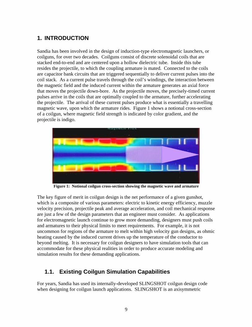
1. INTRODUCTION Sandia has been involved in the design of induction-type electromagnetic launchers, or coilguns, for over two decades. Coilguns consist of discrete solenoidal coils that are stacked end-to-end and are centered upon a hollow dielectric tube. Inside this tube resides the projectile, to which the coupling armature is mated. Connected to the coils are capacitor bank circuits that are triggered sequentially to deliver current pulses into the coil stack. As a current pulse travels through the coil’s windings, the interaction between the magnetic field and the induced current within the armature generates an axial force that moves the projectile down-bore. As the projectile moves, the precisely-timed current pulses arrive in the coils that are optimally coupled to the armature, further accelerating the projectile. The arrival of these current pulses produce what is essentially a travelling magnetic wave, upon which the armature rides. Figure 1 shows a notional cross-section of a coilgun, where magnetic field strength is indicated by color gradient, and the projectile is indigo.

Figure 1: Notional coilgun cross-section showing the magnetic wave and armature

The key figure of merit in coilgun design is the net performance of a given gunshot, which is a composite of various parameters: electric to kinetic energy efficiency, muzzle velocity precision, projectile peak and average acceleration, and coil mechanical response are just a few of the design parameters that an engineer must consider. As applications for electromagnetic launch continue to grow more demanding, designers must push coils and armatures to their physical limits to meet requirements. For example, it is not uncommon for regions of the armature to melt within high velocity gun designs, as ohmic heating caused by the induced current drives up the temperature of the conductor to beyond melting. It is necessary for coilgun designers to have simulation tools that can accommodate for these physical realities in order to produce accurate modeling and simulation results for these demanding applications.

1.1. Existing Coilgun Simulation Capabilities For years, Sandia has used its internally-developed SLINGSHOT coilgun design code when designing for coilgun launch applications. SLINGSHOT is an axisymmetric

10

lumped-parameter circuit code. It models coils as series inductances and resistances (RL) to which a fixed-topology capacitor bank driver is connected. Armature axisymmetric cross sections are meshed into rectilinear elements, which are each treated as an independent RL circuit. Mutual coupling values are calculated between every coil and armature element based on their relative position and stored in a matrix to be used in the electric and mechanical calculations that are performed at each time-step. Figure 2 shows the circuit representation of a single coil stage (capacitor bank and coil) that is mutually coupled to a single armature element [1]. In reality, coupling exists between every inductive element in the simulation: coil to armature, coil to coil, and armature to armature.

Figure 2: SLINGSHOT circuit representation of a coilgun stage coupled to armature element [1]

The subscripted branches in Figure 2 act as placeholders for representations of additional hardware, such as transmission lines between switches and coils, in the driver circuit. Everything within the coilgun system must be lumped within these parameters.

Figure 3: Axisymmetric cross section of coil (green), armature (red) elements in SLINGSHOT [1]

11

Each element is assumed to have uniform current density, so fine meshes are needed to resolve current distributions in the armature cross section. During each time step, the currents in each element are calculated and used along with the mutual inductance information to calculate radial and axial forces per element. These are summed to a single value for the projectile point-mass and used to update its position, velocity, and acceleration information. Projectile motion is only allowed in the forward direction (the positive-z direction in Figure 3). Elements are assumed to be infinitely rigid and material strength properties are not used. The user specifies cross-sectional geometries and materials for coils and armature elements, which the code then uses to establish the equivalent resistances and self-inductances. Based on material specified, a look-up table of resistivity as a function of temperature is used to track conductor resistance of each coil and armature element during ohmic heating. Each element is considered to be adiabatic and when one goes above the assigned material’s melting temperature, it is discarded and ignored for subsequent time-steps within the code.

1.2. The Need for Next Generation Coilgun Simulation Code SLINGSHOT has been a valuable simulation tool for simulating coilgun systems. The previous section was included to highlight the general approach to modeling a coilgun and projectile, with emphasis on the techniques and implementations within SLINGSHOT that limit use of the code to less strenuous gun environments. However, coilguns are always being asked to push harder, go faster, and do so in fewer stages with a shorter axial length. These design goals will cause higher stress environments in which armatures will melt and experience radial magnetic pressure sufficient to cause deformation. In these cases, it becomes essential to capture with high fidelity the mechanical response of these armatures as they are heated and deformed. SLINGSHOT is incapable of satisfactorily accounting for these phenomena, and divergences between simulation and experiment have been seen when they occur. Beyond armature response to the high-stress gun environment, other factors are driving the need to develop a more general simulation tool. The standard topology of an inductive launcher is being expanded upon, no longer thought of as a series of capacitor banks and coil stages. Advanced pulsed power sources, such as rotating energy stores, are being considered for future coilgun designs. There is also a desire to incorporate a larger model of the electrical system, perhaps back to prime power, within a simulation. This all amounts to a need for a more general circuit simulation capability that expands upon the simple series-RLC driver topology found within SLINGSHOT. Further, the inclusion of magnetically permeable materials into a simulation tool’s system of equations is required to develop a modeling capability for shielding experiments, in which Sandia coil systems will be used to impose magnetic field onto devices under test. It is also desired to be able to model systems in which the projectile moves in any of the

12

three translational degrees of motion. This implies expansion from an axisymmetric solution domain to three-dimension simulation space. These are examples of the expansion of the application space to which induction launchers are being designed.

1.3. Case Study: Deformation of 10g armature A brief example of the divergence between reality and SLINGSHOT is provided below. Experimental data has been collected for a single coil system that is used to propel a 10g aluminum slug to 350m/s. Experimental data was collected for various peak currents and tabulated against resulting muzzle velocity, then compared to SLINGSHOT simulations for the same parameters. The data found in Figure 4 shows that as projectiles are radially compressed during launch, SLINGSHOT is unable to account for the subsequent loss of inductive coupling and degrading gun performance.

Simulation Versus Coil Testbed

0

100

200

300

400

500

600

0 5 10 15 20 25 30 35 40 45

Current (kA)

Velo

city

(m/s

)

Simulation -5mm

Experimental -5mm

Simulation 0mm

Experimental 0mm

Figure 4: Simulation and experimental results for 10g aluminum armature

The difference between the two cases is the initial position of the projectile. The distance reference corresponds to the back plane of the armature with respect to the center plane of the coil. The -5mm data corresponds to a projectile that is further down breech initially, and subjected to a longer dwell time within the magnetic field from the current pulse. Significant degraded performance is seen in the -5mm data set at 25kA and above, when the breech corner of the projectile is seen to compress radially inward by over 10% on the diameter. The other dataset, referenced to 0mm, demonstrates this trend is further

13

apparent at higher peak currents. Figure 5 shows pairs of projectiles before and after being launched. When deformation first occurs at lower energies, it does so in an axisymmetric fashion, pinching inward at the rear face. Higher energies and longer dwell time in the -5mm position cause a modal failure in the projectile wall.

Figure 5: Side (top) and breech (bottom) views of unfired (left) and fired (right) projectiles

Early in the program, the multiphysics finite element code ALEGRA was brought to bear to qualitatively explore these results in a 3D simulation. A virtual coil current source was used to simulate the coil, using the actual current waveforms captured during the experimental testing to apply the field boundaries on the armature elements. The projectile was modeled as pure aluminum and no bore tube was present. Though these simplifications prevented reporting anything with quantifiable accuracy, the results revealed that ALEGRA could duplicate the mechanical deformation seen experimentally. We hypothesized that the modal failures seen on the bottom of Figure 5 could be partially attributed to the loose fit of the projectile within the bore: because it sat at the bottom of the bore with a few millimeters of clearance above in the one inch diameter bore, the projectile would be subjected to a non-uniform magnetic field distribution. This would lead to an uneven mechanical loading of the structure. In Figure 6, a rendering of the ALEGRA simulation is given. The initial location of the projectile is positioned to mimic the offset found in the testbed, in which the projectile is moved off of the coil’s coaxial reference by the loose tolerance fit in-bore. This non-axisymmetric initial condition results in non-axisymmetric deformation similar to that seen experimentally.

14

Figure 6: 3D ALEGRA model of single-stage coilgun experiment, with armature deformation

1.4. Xygra: Interfacing Xyce and Alegra for EM Launch applications

Sandia has two internally maintained codes whose capabilities fit perfectly the needs of electromagnetic launch modeling and simulation. Considering again the SLINGSHOT circuit equivalent model for a coilgun stage, seen below in Figure 7, two separate domains are proposed in which each code will operate. On the left and highlighted in red is the capacitor bank driver, which is a specific example of any general circuitry storing the electrical energy that generates the current pulse. It is most desirable to be able to drive a given coil with any arbitrary driver that can be represented by an equivalent circuit. To address this domain, the Sandia Xyce Parallel Electronic Simulator [3] was chosen.

15

Figure 7: Coilgun stage circuit equivalent with domains for Sandia codes highlighted

The section highlighted in blue in Figure 7 represents the physical drive coil and armature, and all mechanical, thermal, and electromagnetic solutions required therein. Sandia’s ALEGRA code [4] is a multiple material, finite element code that emphasizes large deformations in its solution space. Further, it has a robust magnetohydrodynamic modeling capability that is immediately applicable to coilgun inductive coupling. For the scope of this project, it was decided to develop the capability to work within an axisymmetric domain while preparing the path for full three-dimensional simulation. What results are two codes coupled at a two-terminal device interface between these domains. The ALEGRA code models the physical space that the coils and armature inhabit, and Xyce simulates the driver circuitry that generates the current pulses to drive the coils. The codes then need to be coupled to interface at this two-terminal connection. Xyce must provide the initial voltage and current conditions that drive the propulsion coil within ALEGRA space. There, ALEGRA uses this information to fully solve for the magnetic, thermal, and mechanical responses of the modeled geometry. Any projectile movement, whether it be deformation or travel down-bore, changes the magnetic field solution and effective circuit properties of the coil, necessitating an update to the voltage and current parameters at the two-terminal interface. ALEGRA updates these values at the end of its iteration and passes back the incremented circuit parameters to Xyce, who then iterates its transient solution to the driver circuitry. Both Xyce and ALEGRA require significant added capabilities to make them usable in an EM launch application. Xyce circuit models needed to be modified for coilgun-specific phenomena, such as position-dependent mutual inductance coupling coefficients and resistors whose value changes as a function of temperature. The ALEGRA source code requires development of the circuit coupled coilgun modeling capability, to handle driving conserved current between otherwise isolated coil windings in the simulation. Finally, a tandem coding effort is required to allow calling of Xyce as a Third Party Library (TPL) from within ALEGRA to handle the handshake of simulation parameters across the two terminal device between time steps.

16

Given this capability, there are two distinct approaches we want when attempting to simulate coilgun launch. The first, as outlined above, represents a high-fidelity, computationally intensive approach. With the changes undertaken for some Xyce component models to be compatible with ALEGRA, it was not difficult to extend this work into generating a rapid prototyping tool that is entirely Xyce-based. This capability is essentially a retread of the circuit equivalencies for a coilgun found within SLINGSHOT, but with the added capability to use arbitrary coil driver circuits. Figure 8 graphically details the two approaches that can be taken with these developed tools. One can envision multiple iterations in the rapid engineering cycle to narrow down the parameter space for a design before generating a higher-fidelity simulation in the path on the right.

Figure 8: Flowchart of two paths available for modeling coilguns with Xyce and ALEGRA codes

17

2. UPDATES AND USAGE OF XYCE FOR EM LAUNCH APPLICATIONS

2.1. Update of device models in Xyce To use Xyce for rapid prototyping simulation of coilgun problems, a number of new or updated device models were required. They are:

Self-consistent integration of projectile dynamics with circuit solution: A second-order ODE was integrated into the full system of differential-algebraic equations being solved for the circuit itself. Since the position of the projectile is used elsewhere in the circuit (to compute mutual inductance between projectile armature and drive coil), self-consistency of the solution is essential, and is provided by using the same solver for the whole problem.

Mutual inductance with time- and solution-dependent coupling coefficients: The normal SPICE mutual inductor assumes a constant coupling coefficient in the linear mutual inductor. In order to capture the coupling between a moving armature and a fixed launch coil, this feature had to be modified to allow time-varying coupling coefficients. Allowing a time-dependent coupling adds additional time-derivative terms to the set of equations solved by the circuit solver, and allowing the coupling coefficient to depend on other solution variables (such as projectile location) requires additional modifications to assure consistency in the nonlinear system of differential-algebraic equations solved by Xyce.

Thermal Resistor: A resistor model including self-heating effects was incorporated into Xyce, to account for changes in resistance (as defined by a material’s temperature coefficient of resistivity) as the coils and armature elements are subjected to substantial ohmic heating.

2.2. Rapid Coilgun Prototyping with Xyce: A Users' Guide Simulation of coilguns in Xyce is done by casting the problem into a circuit-like description known as a netlist, which defines the connectivity between the circuit elements. In the sections that follow, we describe the steps one would take to design a netlist to simulate a coilgun with a single drive coil and a projectile with a single armature element. We will then describe the additional steps needed to add drive coils, and outline the further steps involved in designing a netlist with more than one armature element. Netlist construction for a single-drive-coil coilgun In the following sections, we will construct a netlist to simulate a coilgun with a single drive coil and a single armature. The drive coil will have an inductance of 13.68855mH, and the armature coil will have an inductance of 94.31303nH. The drive circuitry will contain switches that will close at a time dependent on projectile position and velocity, and turn off at a specified time.

18

Mutual Inductance Tables Before simulation with Xyce can proceed, tables must be generated of mutual inductance and mutual inductor coupling coefficients between armature and drive coils, as functions of the distance between them. This is accomplished by a MATLAB routine that calculates element resistance and inductance values based on element input geometry. These calculations are themselves based off of Lyle’s method found in Grover [2] and identical to the methodology used in the solution found within SLINGSHOT. These scripts tabulate look-up tables as function expressions that Xyce uses to construct a piecewise linear function for the mutual inductance and coupling coefficients. For the simple single-coilgun under consideration, the scripts will produce a file containing the following lines:

.PARAM LM1_1 = 9.431303e-008

.PARAM KM1_1 = 0

.PARAM LM2_2 = 1.368855e-002

.PARAM KM2_2 = 0

.FUNC LMz1_2(x) {TABLE(x, +-1.562200e-001,3.430407e-006, +-1.504200e-001,3.702524e-006, [...] +)} .FUNC KMz1_2(x) {TABLE(x, +-1.562200e-001,9.547309e-002, +-1.504200e-001,1.030465e-001, [...] +1.511800e-001,8.300322e-002, +)}

This file defines a parameter for each of the individual coil inductances, and a piecewise-linear function for mutual inductance (LMz1_2(x)) as a function of armature-coil distance. The function KMz1_2(x) is the mutual inductance coupling coefficient as a function of armature-coil distance, x. The mutual inductance M between inductors of inductance L1 and L2 is related to the coupling coefficient k by 21LLkM = . In the tables, the first column is the value of x and the second the value of the function at x. When called with a given value of x, Xyce performs linear interpolation between the specified values. Netlist specification of coil drive circuitry For ease of re-use, the drive circuitry will be set up as a parameterized subcircuit. When defined this way, the subcircuit can be instantiated multiple times with different parameters; this will come in handy when we progress to multiple-coil devices. The subcircuit is a realization of the same circuit found in Figure 7 to allow for direct comparison with SLINGSHOT results.

Subcircuits in Xyce netlists are defined between “.subckt” and “.ends” lines. The .subckt line defines the name of the subcircuit, its connection ports, and its parameters. We will define a subcircuit with connection ports for the drive coil and also ports for passing in

19

the position and velocity of the projectile. The parameters will be the position of the coil along the gun axis and the component values of all inductors, capacitors, and resistors in the drive circuit.:

.subckt DriveCoil L1 L2 z dzdt PARAMS: pos=0 c=2m Ra=10m Rb=50m

+ Rd=1m La=100nH Lb=10uH Lc=10mH Ld=100nH

This subcircuit declaration defines a subcircuit named “DriveCoil” that is connected via four ports: L1 and L2 for the drive coil, and additional nodes z and dzdt for the projectile position and velocity. The list of parameters after “PARAMS:” defines both the names of parameters we may pass to the subcircuit when we instantiate it, and the default values of any parameters that are left unspecified by the instantiation. Lines beginning with “+” are continuation lines in netlists, so the two text lines above are considered a single “.subckt” line. Following the .subckt declaration line, we specify the components of the subcircuit and their connections, and end the subcircuit definition with an “.ends” line:

Vc L1 4 0 Rc 9 L2 290m Rd 8 9 {Rd} Ld 7 8 {Ld} Sw1 1 7 SW_ideal control={if(pos=0,time/Stime, + (1e-20+v(z)-pos+lead*riseTime*v(dzdt))/ + (if(time>0.0001,v(dzdt)*Stime,1)))} Lb 6 7 {Lb} Sw2 5 6 SW_ideal control={switch_2_off} Rb 4 5 {Rb} La 2 1 {La} C 2 3 {C} ic=5K Ra 4 3 {Ra} Rgnd 0 L1 1e+6 .ends DriveCoil .model SW_Ideal VSWITCH (ROFF=1meg RON=1m OFF=0 ONE=1)

Each line of the specification defines a circuit element, which is followed by some number of voltage nodes at the element's terminals. Component values that are specified in terms of subcircuit parameters are enclosed in curly braces ({}). The capacitor “C” is given an initial condition of 5KV --- this is the voltage across the capacitor at the beginning of the simulation, indicating that it is charged. Switch Sw1 is controlled by an expression dependent on the position of the coil, the position and velocity of the projectile, the current time, and a number of parameters we have not yet defined. The switch is “closed” when the expression is greater than one and “open” when the expression is less than zero. In between those values the resistance of the switch is smoothly varying between its open and closed values. The on and off resistances and control values are specified in the “.model” statement defining the “SW_Ideal” switch model. Consult the Xyce Users Guide [3] for a detailed explanation of the general switch model and netlist expressions.

20

As specified here, we have only defined the subcircuit in terms of parameters and unspecified connections. In this way it is like declaring a subroutine in a program. To use the subcircuit we have to instantiate it in the netlist. This is done by adding an “X” line to the netlist, which serves as a “subroutine call” and specifies the connections to other devices:

XCoil2 11_2 10_2 z dzdt DriveCoil PARAMS: pos=0 c=4m Ra=10m + Rb=50m Rd=1m La=100nH Lb=10uH Lc={LM2_2} Ld=100nH

This line defines an instance of a coil-drive subcircuit where the coil is meant to connect to nodes 11_2 and 10_2, and most of the parameters are set to their default values. Subcircuit parameter “Lc”, which is used only in computation of the parameter “riseTime” is set to match the inductance of the drive coil that was computed by MATLAB and stored in the inductance file. Netlist specification of Drive Coil The drive coil itself is simply an inductor whose inductance is given by the parameter LM2_2 as defined in the inductance file produced by the MATLAB scripts. It is specified in the netlist by a single “L” line:

Lc_2 11_2 10_2a {LM2_2} Rc_2 10_2a 10_2 100m

This line defines an inductor connected between the nodes of the drive circuitry, with an inductance as given by the parameter LM2_2. A series resistor is included per coil to account for the finite conductivity of the coil winding material. Netlist specification of armature The armature will be modeled by a small circuit containing an inductor, a resistor, and an ammeter (from which we can extract the current value we will need to compute forces). In order for the Xyce circuit solver to converge properly, this armature will have to have an artificial connection to ground through a large (1MOhm) resistor.

Lp A_1 0p {LM1_1} Rp A_1 A_1b 0.000012 Vp A_1b 0p 0 RPgnd 0p 0 1e+6

The zero-volt voltage source Vp allows us access to the current through the armature winding. This will be used together with the current in the drive coil and the LMz1_2 function to compute the force between the projectile and drive coil. Netlist specification of drive-coil/armature coupling Changing currents in the drive coil induce currents in the armature; this is the essential property that allows coilguns to generate thrust. This coupling is specified through the Xyce mutual inductor device.

K_1_2 Lp Lc_2 {KMz1_2(v(z)+Poff)}

This mutual inductance line specifies that the inductors Lp in the projectile and the Lc_2 drive coil are coupled with a coupling coefficient that depends on the position of the armature. The position of the projectile is given by the value of the voltage at node z,

21

which is accessed as “v(z)” in the expression. The projectile position is not necessarily the position of the armature, as the armature may be offset from the back of the projectile. We use a defined parameter “Poff” to allow for this offset. This parameter will be defined elsewhere in the netlist. The function KMz1_2(x) is the one from the inductance file produced by the MATLAB scripts, and gives the coupling coefficient between the two inductors Lp and Lc_2. Netlist specification of coil/armature forces and projectile kinematics The force between the drive coil and the armature coil is given by

dzdMIIF ca

ac=

This force is computed in Xyce using a “B” source (analog behavioral modeling source) to provide a fictitious voltage at a circuit node that can then be used to provide the acceleration, to be integrated to yield projectile velocity and position.

Bacc acceleration 0 V={( + I(Vp)*I(XCoil2:Vc)*ddx(LMz1_2(v(z)+Poff),v(z)) + )/mass}

This line defines the node “acceleration” and requires that the voltage between that node and ground be the voltage as specified by the expression in curly braces, which is just the force as given above divided by the projectile mass (which is yet to be defined). Since this voltage source is not yet connected to anything it does not define a proper circuit element, so we provide a resistor to ground so that the circuit is complete:

Racc acceleration 0 1 Finally we must specify that the acceleration be integrated twice to obtain the position and velocity of the projectile. This is done using the YACC “accelerated mass device”:

YACC acc1 acceleration dzdt z v0=0 x0=0 This device adds the second-order initial value problem of projectile kinetics to the set of equations that Xyce will solve. The voltage at node z will be the position and the voltage at node dzdt will be the velocity. Because this YACC device is a specialized device written for this project precisely to compute the solutions of kinematics problems, it is not a voltage source the way that the general Xyce B source circuit element is; these “voltage” nodes do not need to be connected to ground for convergence's sake. Complete Netlist The steps we have taken so far have constructed netlist fragments that need to be assembled with additional information to make a complete input file for Xyce. The completed netlist, with parameter definitions, simulator directives, and comments is given below.

*Sample coilgun netlist * Include the MATLAB-generated inductance file:

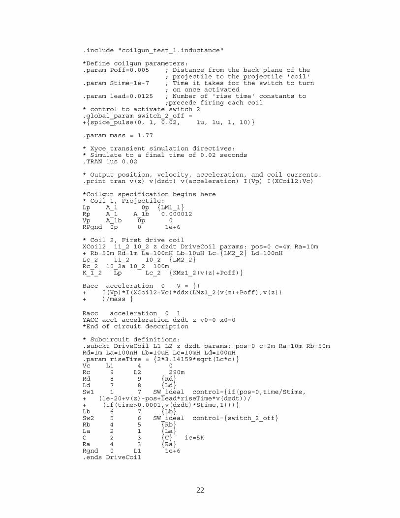
22

.include "coilgun_test_1.inductance" *Define coilgun parameters: .param Poff=0.005 ; Distance from the back plane of the ; projectile to the projectile 'coil' .param Stime=1e-7 ; Time it takes for the switch to turn ; on once activated .param lead=0.0125 ; Number of 'rise time' constants to ;precede firing each coil * control to activate switch 2 .global_param switch_2_off = +{spice_pulse(0, 1, 0.02, 1u, 1u, 1, 10)} .param mass = 1.77 * Xyce transient simulation directives: * Simulate to a final time of 0.02 seconds .TRAN 1us 0.02 * Output position, velocity, acceleration, and coil currents. .print tran v(z) v(dzdt) v(acceleration) I(Vp) I(XCoil2:Vc) *Coilgun specification begins here * Coil 1, Projectile: Lp A_1 0p {LM1_1} Rp A_1 A_1b 0.000012 Vp A_1b 0p 0 RPgnd 0p 0 1e+6 * Coil 2, First drive coil XCoil2 11_2 10_2 z dzdt DriveCoil params: pos=0 c=4m Ra=10m + Rb=50m Rd=1m La=100nH Lb=10uH Lc={LM2_2} Ld=100nH Lc_2 11_2 10_2 {LM2_2} Rc_2 10_2a 10_2 100m K_1_2 Lp Lc_2 {KMz1_2(v(z)+Poff)} Bacc acceleration 0 V = {( + I(Vp)*I(XCoil2:Vc)*ddx(LMz1_2(v(z)+Poff),v(z)) + )/mass } Racc acceleration 0 1 YACC acc1 acceleration dzdt z v0=0 x0=0 *End of circuit description * Subcircuit definitions: .subckt DriveCoil L1 L2 z dzdt params: pos=0 c=2m Ra=10m Rb=50m Rd=1m La=100nH Lb=10uH Lc=10mH Ld=100nH .param riseTime = {2*3.14159*sqrt(Lc*c)} Vc L1 4 0 Rc 9 L2 290m Rd 8 9 {Rd} Ld 7 8 {Ld} Sw1 1 7 SW_ideal control={if(pos=0,time/Stime, + (1e-20+v(z)-pos+lead*riseTime*v(dzdt))/ + (if(time>0.0001,v(dzdt)*Stime,1)))} Lb 6 7 {Lb} Sw2 5 6 SW_ideal control={switch_2_off} Rb 4 5 {Rb} La 2 1 {La} C 2 3 {C} ic=5K Ra 4 3 {Ra} Rgnd 0 L1 1e+6 .ends DriveCoil

23

*Switch model definition .MODEL SW_Ideal VSWITCH (ROFF=1meg RON=1m OFF=0 ON=1) .end

Additional netlist considerations for multiple drive coils The netlist in the previous section contains the essential elements of any coilgun Xyce simulation: drive-coil circuitry, drive coils, armature coils, coupling between drive and armature, and force computation. Adding additional drive coils introduces only a little complexity.

Because we created a parameterized drive subcircuit (and could create more templates as needed), we can add additional drives with relative ease, changing only the parameters and connection nodes. But for each drive coil added there are additional mutual inductors to add: one mutual inductor for each previous drive coil, coupling the new drive coil to the previous, and an additional mutual inductor coupling the new drive coil to the armature. The B source that computes the force on the armature will now have additional terms due to the additional drive coils.

The single-coil drive circuit in the previous netlist may be augmented to a two-coilgun simulation by adding one additional drive circuit, an additional drive coil, and two additional mutual inductors, and by modifying the acceleration computation.

The MATLAB pre-processor script will generate additional functions for the new mutual inductances, and these will be included in the inductance file. The inductance of the second drive coil (LM3_3) and the constant coupling coefficient between the first and second drive coils (KM2_3) will be computed by the scripts and included in the inductance file as well.

The second drive circuit is introduced by creating a second instantiation of the drive subcircuit with a different position (as defined by the parameter “Zspace”) and different Lc value:

XCoil3 11_3 10_3 z dzdt DriveCoil params: pos=Zspace c=2m Ra=10m + Rb=50m Rd=1m La=100nH Lb=10uH Lc={LM3_3} Ld=100nH

It is followed by specification of the second drive coil and the coupling of the second drive coil to the first drive coil and the armature:

Lc_3 11_3 10_3 {LM3_3} K_1_3 Lp Lc_3 {KMz1_3(v(z)+Poff-Zspace)} K_2_3 Lc_2 Lc_3 {KM2_3}

Finally, the Bacc voltage source is replaced with a new one:

Bacc acceleration 0 V = {( + I(Vp)*I(XCoil2:Vc)*ddx(LMz1_2(v(z)+Poff),v(z)) + + I(Vp)*I(XCoil3:Vc)*ddx(LMz1_3(v(z)+Poff-Zspace),v(z)) + )/mass }

As before, this B source sets the voltage at node “acceleration” to be the force on the projectile divided by the mass, but now the force is the sum of the forces generated by the

24

two drive coils. For numerical stability, when actually placed in the netlist the common factor I(Vp) is factored out and the B source is defined as:

Bacc acceleration 0 V = {( + I(Vp)*(I(XCoil2:Vc)*ddx(LMz1_2(v(z)+Poff),v(z)) + + I(XCoil3:Vc)*ddx(LMz1_3(v(z)+Poff-Zspace),v(z))) + )/mass }

These changes lead to a completed netlist that is given below:

* Two-coil coilgun * The inductance file must be regenerated by MATLAB .include "coilgun_test_1.inductance" .param Poff=0.005 ; Distance from the back plane of the ; projectile to the projectile 'coil' .param Zspace=0.0707 ; Spacing of the drive coils .param Stime=1e-7 ; Time it takes for the switch to turn on ; once activated .param lead=0.0125 ; Number of 'rise time' constants to ; precede firing each coil * control to activate switch 2 .global_param switch_2_off = {spice_pulse(0, 1, 0.02, 1u, 1u, 1, 10)} .param mass = 1.77 ; projectile mass .TRAN 0 0.02 .print tran v(z) v(dzdt) v(acceleration) I(Vp) I(XCoil2:Vc) I(XCoil3:Vc) * Coil 1, Projectile: Lp A_1 0p {LM1_1} Rp A_1 A_1b 0.000012 Vp A_1b 0p 0 RPgnd 0p 0 1e+6 * Coil 2, First drive coil XCoil2 11_2 10_2 z dzdt DriveCoil params: pos=0 c=4m Ra=10m + Rb=50m Rd=1m La=100nH Lb=10uH Lc={LM2_2} Ld=100nH Lc_2 11_2 10_2 {LM2_2} K_1_2 Lp Lc_2 {KMz1_2(v(z)+Poff)} * coil 3: second drive coil XCoil3 11_3 10_3 z dzdt DriveCoil params: pos=Zspace c=2m Ra=10m + Rb=50m Rd=1m La=100nH Lb=10uH Lc={LM3_3} Ld=100nH Lc_3 11_3 10_3 {LM3_3} K_1_3 Lp Lc_3 {KMz1_3(v(z)+Poff-Zspace)} K_2_3 Lc_2 Lc_3 {KM2_3} * General coil. Note that param values listed here are defaults. * The actual values used should be specified in the subcircuit * call line (XCoil...) .subckt DriveCoil L1 L2 z dzdt params: pos=0 c=2m Ra=10m Rb=50m + Rd=1m La=100nH Lb=10uH Lc=10mH Ld=100nH .param riseTime = {2*3.14159*sqrt(Lc*c)} Vc L1 4 0 Rc 9 L2 290m Rd 8 9 {Rd} Ld 7 8 {Ld} Sw1 1 7 SW_ideal control={if(pos=0,time/Stime, + (1e-20+v(z)-pos+lead*riseTime*v(dzdt))/

25

+ (if(time>0.0001,v(dzdt)*Stime,1)))} Lb 6 7 {Lb} Sw2 5 6 SW_ideal control={switch_2_off} Rb 4 5 {Rb} La 2 1 {La} C 2 3 {C} ic=5K Ra 4 3 {Ra} Rgnd 0 L1 1e+6 .ends DriveCoil Bacc acceleration 0 V = {( + I(Vp)*(I(XCoil2:Vc)*ddx(LMz1_2(v(z)+Poff),v(z)) + + I(XCoil3:Vc)*ddx(LMz1_3(v(z)+Poff-Zspace),v(z))) + )/mass } Racc acceleration 0 1 YACC acc1 acceleration dzdt z v0=0 x0=0 .MODEL SW_Ideal VSWITCH (ROFF=1meg RON=1m OFF=0 ON=1) .end

Additional coils may be added in a similar manner. The number of mutual inductor devices will grow rapidly, as will the number of tables that will need to be generated by MATLAB scripts. Netlist considerations for multiple armature elements The netlists presented so far all assume a single armature element with a single inductance, and both of the netlists above have been run in Xyce exactly as presented here. To date, no attempt has been made to generate and run a coilgun simulation in Xyce with an armature of more complexity, but nothing in the formulation prohibits using Xyce to simulate a more complex armature model with multiple elements. We present below some guidance on how multiple armature elements would be modeled, with the understanding that netlist fragments presented here have not been tested in real simulations.

In the single-armature-element simulation, the armature is modeled as a single inductor, resistor, and current-measuring voltage source. To model multiple armature elements would require additional instances of this pattern.

*First armature element coil “P1” Lp1 A_1 0p1 {LM1_1} Rp1 A_1 A_1b 0.000012 Vp1 A_1b 0p1 0 RPgnd1 0p1 0 1e+6 *second armature element coil “P2” Lp2 A_2 0p2 {LM2_2} Rp2 A_2 A_2b 0.000012 Vp2 A_2b 0p2 0 RPgnd2 0p2 0 1e+6

Here an additional parameter LM2_2, the inductance of the second armature element, must be computed in the MATLAB scripts.

The presence of a second armature element introduces a new coupling: varying currents in one armature element will induce currents in the other. Hence there will be an

26

additional mutual inductor device with a newly-defined constant coupling KM_p1_p2 that must be computed by MATLAB and defined in the inductor file:

KP1_P2 Lp1 Lp2 {KM_p1_p2}

Each armature element will be coupled further to all drive coils, so the full list of mutual inductors for a single-drive-coilgun would be

K_p1_2 Lp1 Lc_2 {KMzp1_2(v(z)+Poff1)} K_p2_2 Lp2 Lc_2 {KMzp2_2(v(z)+Poff2)}

Here we have adopted the convention that coils in the projectile are labeled “Pn” and drive coils are numbered as they were before (beginning at coil 2, since our original single-armature element netlist named the armature “coil 1”). Here we see that we now require two mutual inductor coupling coefficient functions, one for each armature element. The total number of these coupling functions will be the product of the numbers of armature elements and drive coils. Note also that there are two offset constants, each giving the offset of the armature element from the back of the projectile. Finally, the force on the projectile is now the sum of the forces on the armature elements. For a single drive coil our “Bacc” device becomes:

Bacc acceleration 0 V = {( + I(Vp1)*I(XCoil2:Vc)*ddx(LMzp1_2(v(z)+Poff1),v(z)) + + I(Vp2)*I(XCoil2:Vc)*ddx(LMzp2_2(v(z)+Poff2),v(z)) + )/mass }

Here again we see the need for a second mutual inductance table corresponding to our second coupling coefficient table. Again we will need a total number of mutual inductance functions equal to the product of the numbers of armature elements and drive coils. For multiple drive coils there will also be mutual inductors coupling every pair of drive coils, precisely as we had early for the two-drive/one-armature simulation. Netlist considerations for incorporating self-heating effects Heating of the projectile due to ohmic losses, and the corresponding effect of that heat on the resistance of the projectile, is an important effect in coilgun operation that is not captured by any of the netlists presented so far. To capture this effect, a new resistor model was added to Xyce for this project, the level 2 thermal resistor. This device provides a variable resistance; the resistance at any time is a function of the temperature of the resistor, and the heating of the resistor due to ohmic losses causes a change in the resistor's temperature over time.

The level 2 resistor in Xyce allows the user to specify the resistivity and heat capacity of the material from which the resistor is made. These are specified in a “.model” statement. Specifications of the length and cross-sectional area of the resistor complete the description. A simple netlist that runs a constant 5-volt source across a thermal resistor would be:

*Thermal resistor example

27

.model copper r (level=2 + resistivity={table(temp+273.15, + 0, 0.5e-9, + 100, 3.0e-9, + 1000, 6.6e-8)} * 8.92e+3 is the density of copper in kg/m**3. Tabulated * function is in Joule/degree K/kg, so product is heat capacity * in Joule/degree K/m**3 + heatcapacity={8.92e+3*table(temp+273.15, + 0, 1, + 1000, 1500)} + ) R1 1 0 copper L=0.1 a=1e-5 V1 1 0 5 .tran 0 1 .print tran R1:R R1:TEMP I(R1) .end

This netlist defines a .thermal resistor model called “copper” with specified resistivity and heat capacity functions. The functions are piecewise linear and are specified as tables with the first column being degrees Kelvin and the second being the function value; the temperature is stored internally in Xyce in degrees Celsius, so a conversion is done in the netlist. This model is then used in a resistor instantiation R1 to define a .1m wire of cross sectional area 1e-5m2. This resistor is attached to nodes 1 and 0 of the circuit, and uses the previously-defined “copper” model. The voltage source V1 provides a constant potential of 5 volts between nodes 1 and 0. The simulation begins with the resistor's temperature at the default ambient temperature of 27 degrees Celsius and allows the current to heat the resistor (thereby increasing its resistance and its self-heating) for one second. The netlist prints the resistance, temperature, and current through resistor R1 at each time step. Given the parameters specified above, at the end of the one-second simulation the temperature of the resistor is nearly 3250 degrees. Since this temperature exceeds the tabulated values of resistivity and heat capacity, it is unlikely to be very accurate; tabulating the functions for the full range of expected values would be necessary. Replacing the constant resistor Rp in the armature model with an appropriately designed thermal resistor model would allow simulation of the self-heating of the projectile material in a coilgun shot. To do so would require specification of the resistivity function and heat capacity functions. There are additional parameters available for defining thermal resistors, and these are enumerated in the Xyce Reference Guide for Xyce Release 4.1, to be released after this paper’s publishing.

2.3. Changes to Xyce for use as TPL for ALEGRA Coupling Xyce is primarily intended as a stand-alone application, but has been adapted to serve as an external library for a number of other applications. To prepare for coupling to ALEGRA, a small number of additional classes and API methods were added. The source code incorporating these changes has been added to the ALEGRA/Nevada repository and it is now included in the third party library set for use in ALEGRA. The classes added are:

28

N_CIR_Xygra: This is the primary class that will be used by ALEGRA. All Xygra-specific API calls are methods of this class.

N_DEV_Xygra: This class defines a new device type (”YXYGRA”) for use in netlists. It receives parameters from ALEGRA simulations through the API methods of N_CIR_Xygra. At this time, the Xygra device provides an interface to the circuit that appears as an N-terminal device, with each pair of terminals simulating a single coil of some number of windings. The currents in the windings of each coil are functions of nodal voltages and parameters computed by and passed in from ALEGRA.

Additional internal modifications of the device interface and device manager packages were required to implement the API methods.

2.4. Xyce Perspective of Xyce / ALEGRA Integration From the circuit point of view, the “YXYGRA” device is simply a circuit element that adds current contributions to the differential-algebraic system resulting from a modified nodal analysis of the circuit. At each time integration step, Xyce solves for the set of voltages that satisfy Kirchhoff's voltage and current laws using a Newton-Raphson nonlinear solver. Currents in the Xygra device are computed as a function of nodal voltages using parameters provided by ALEGRA; these parameters are given as an S vector and K matrix as discussed in a later section of this document. At each of ALEGRA's time steps, ALEGRA will query Xyce for nodal voltages in the Xygra device, which it will use as boundary conditions for its solution of the electromagnetics part of the computation. From its solution, ALEGRA will compute these Xygra device parameters and pass them back to Xyce, which will be asked to integrate forward in time to the end of the time step specified by ALEGRA. The process repeats with alternating ALEGRA and Xyce time-stepping until the full simulation time is complete. The single-drive-coil Xyce netlist given earlier would have only minor modifications to be used in this framework. The armature and drive coils would be replaced by a single Xygra device, and the YACC accelerated mass device would be replaced by another Xygra device. Thus, the main top-level circuit (neglecting parameter and subcircuit definitions) would be:

* Coil 2, First drive coil XCoil2 11_2 10_2 z dzdt DriveCoil params: pos=0 c=4m Ra=10m + Rb=50m Rd=1m La=100nH Lb=10uH Lc={LM2_2} Ld=100nH YXygra CoilGun 11_2 10_2 + coil={NAME=coil1 + WINDINGS=40} YXygra Kinematics Z 0 DZDT 0 + coil={NAME=position,velocity + WINDINGS=1,1} Rz Z 0 1 Rdzdt DZDT 0 1

29

In this netlist fragment, the drive circuitry is precisely as it was in the Xyce-only simulation. The armature (those components in “Coil 1”), drive coil Lc_2, and mutual inductor K_1_2 have been replaced by the Xygra device “YXYGRA CoilGun” which is specified as having a single 40-winding coil for example's sake. It is to this device that ALEGRA will provide the S vector and K matrix for simulation of the coilgun's electrical coupling to the circuit. Actual simulation of the projectile and coil windings will be done in ALEGRA using boundary conditions obtained from the circuit simulation. In addition, position and velocity of the projectile are fed from ALEGRA to Xyce through a second Xygra device, “YXYGRA Kinematics.” In this instance, ALEGRA will simply load the S vector parameter with the position and velocity, which Xyce will treat as current sources through fictitious single-winding coils; the K matrix will be left unspecified, signifying no dependence of the current on the voltage across these fictitious coils. These currents are run through 1-ohm resistors to ground, so the corresponding nodes will have a voltage equal to position and velocity. These nodal voltages may then be used in the drive coil switch expressions where position and velocity are needed. The “YXYGRA Kinematics”, Rz, and Rdzdt devices replace the “YACC acc1”, “Bacc” and “Racc” devices in the original circuit. This second Xygra device addresses the active feedback requirement mentioned in point (4) in the list found in section 3.3 below describing the ALEGRA development. Multiple-drive-coil coilguns would be simulated in a similar fashion, with multiple coil driver subcircuit instantiations, but with a Xygra device with more than one pair of connecting nodes, and more than one coil. For example, a two-coilgun would be specified as:

* Coil 2, First drive coil XCoil2 11_2 10_2 z dzdt DriveCoil params: pos=0 c=4m Ra=10m + Rb=50m Rd=1m La=100nH Lb=10uH Lc={LM2_2} Ld=100nH * Coil 3, second drive coil XCoil3 11_3 10_3 z dzdt DriveCoil params: pos=Zspace c=4m Ra=10m + Rb=50m Rd=1m La=100nH Lb=10uH Lc={LM3_3} Ld=100nH YXygra CoilGun 11_2 10_2 11_3 10_3 + coil={NAME=coil2,coil3 + WINDINGS=40,40} YXygra Kinematics Z 0 DZDT 0 + coil={NAME=position,velocity + WINDINGS=1,1} Rz Z 0 1 Rdzdt DZDT 0 1

Note that here the “YXYGRA CoilGun” device now has four nodes and specification of two coils (here both with 40 windings for example's sake). The API of the N_CIR_Xygra class provides the following methods that will be used by ALEGRA:

initialize(int argc, char** argv): This method initializes the N_CIR_Xygra object with the equivalent of a set of command-line arguments. In common usage, the only argument provided will usually be the name of a netlist file.

getDeviceNames(const string & deviceType, vector<string> & deviceNames): This method returns a vector of the names of all devices of the specified type that

30

appear in the netlist. This method will be used to obtain number of Xygra devices in use and their names.

xygraGetCoilWindings(const string & deviceName,vector<int> & coilWindings): Given a named Xygra device, this method returns a vector whose length is the number of coils in the device. The elements of the vector are the numbers of windings in each coil.

xygraSetSources(const string & deviceName, vector<double> S, double t) and xygraSetK(const string & deviceName, vector<vector<double> >K, double t): These methods pass the vector and matrix parameters needed for current computation from ALEGRA to the Xygra device. These are interpolated between values given at the beginning and end of the ALEGRA time step, as Xyce is likely to take several circuit time steps for each of the electromagnetic time steps.

int xygraGetNumNodes(const string & deviceName): returns the number of voltage nodes in the named Xygra device. Each coil has a number of nodes equal to one more than its number of windings. xygraGetNumNodes returns the total number of nodes in all coils of the named device.

int xygraGetNumWindings(const string & deviceName): Returns the total number of windings in the named device. Unlike xygraGetCoilWindings, the returned value is the sum of windings over all coils in the device.

simulateUntil(double untilTime,double & completedTime): resumes the circuit simulation from the last time simulated until the time specified by untilTime, returning the time reached in completedTime. If the simulation has not yet been started, it will be started by this call. When untilTime is reached, the simulation will be paused and control returned to the caller.

xygraGetVoltages(const string & deviceName, vector<double> &V): Returns a vector V containing the voltages on all the nodes in the named device.

simulationComplete(): This method returns true if Xyce has simulated the circuit up to the maximum time specified in the associated netlist. Further calls to simulateUntil made after simulationComplete returns will have no effect. Returns false if the end time specified in the netlist has not yet been reached.

2.5. Current Status of Modifications to Xyce Code

The tools for rapid prototyping of coilgun designs in Xyce are in place and robust. These features of Xyce are part of production releases and are subject to regular regression testing. Initial simulations using the rapid prototyping tool have been performed and are currently being compared against SLINGSHOT results for the same geometry. Figure 9 shows a sample Xyce-produced velocity profile for a single armature element propelled by five drive coils. The flat-top at the end of the simulation indicates the premature end of the look-up mutual inductance table described in section 2.2; the dM/dz tables are forced to zero at a certain axial distance from the coil, resulting in no additional acceleration on the projectile. Shortly, these results will be compared against a similar SLINGSHOT simulation to evaluate the accuracy of the Xyce rapid prototyping tool.

31

Figure 9: Initial Xyce coilgun simulation results for a five-coil, single armature element case

Coupling between Xyce and ALEGRA is still under development. ALEGRA has successfully simulated coilgun problems with imposed voltage boundary conditions and with circuit coupling using its internal DASPK-based circuit solver. The Xygra API and Xygra device have been implemented, and integration with ALEGRA has begun. An alpha-quality code integration will be complete by the end of the FY08 and an example calculation of a single-coil launch demonstrating code coupling will be run soon after. It is not yet known whether this loose coupling between Xyce and ALEGRA will be sufficiently accurate for coilgun modeling needs. Furthermore, discontinuities on the circuit side (as, for example, during switch closures) complicate the loose coupling. It is possible that a tighter coupling of the systems will be necessary, but this has not yet been investigated. Further refinements of the model, API, and coupling strategy will certainly be needed, and a clean user interface for specifying coupled simulation must be developed.

3. DEVELOPING CIRCUIT COUPLED COILGUN MODELING IN ALEGRA

ALEGRA is a multi-physics arbitrary Lagrangian-Eulerian (ALE) modeling code. The code has an extensive history in modeling flyer plates for magnetically driven equation of state studies and other 2D and 3D magnetohydrodynamic problems. The code has a successful history of coupling with external circuits through boundary conditions linearly

32

related to currents or voltage drops across a single power flow gap. The prime example of this usage is for flyer plates modeling in which the anode and cathode gap of the Z-machine at Sandia is modeled using the 2D x-y MHD version of Alegra. In these problems there is one region which represents the cathode side and one region which represents the anode side and the sum of the currents in these two regions is zero since they are assumed to be shorted at the bottom of the load. All of the applications of Alegra-MHD so far have only a single entry and exit point of the current. In contrast, the quasi-static electric field version of ALEGRA which models dielectric systems supports multiple constant potential surfaces and the coupling matrix which relates them. In analogy, it is clear that in moving ALEGRA into the coilgun modeling arena, the methodology for circuit coupling must be generalized to naturally support multiple current entry and exit points. We describe our current approach and results for 2D axisymmetric modeling. The ALEGRA methodology is to split operators in which the mesh moves to understand thermal and magnetics stresses, and magnetic and thermal diffusion is implemented as a separate operator split step. A local remesh and a remap of dependent variables is possible as well.

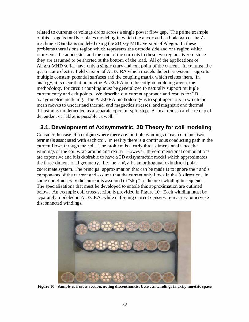
3.1. Development of Axisymmetric, 2D Theory for coil modeling Consider the case of a coilgun where there are multiple windings in each coil and two terminals associated with each coil. In reality there is a continuous conducting path in the current flows through the coil. The problem is clearly three-dimensional since the windings of the coil wrap around and return. However, three-dimensional computations are expensive and it is desirable to have a 2D axisymmetric model which approximates the three-dimensional geometry. Let the ,,r zθ be an orthogonal cylindrical polar coordinate system. The principal approximation that can be made is to ignore the r and z components of the current and assume that the current only flows in the θ direction. In some undefined way the current is assumed to "skip" to the next winding in sequence. The specializations that must be developed to enable this approximation are outlined below. An example coil cross-section is provided in Figure 10. Each winding must be separately modeled in ALEGRA, while enforcing current conservation across otherwise disconnected windings.

Figure 10: Sample coil cross-section, noting discontinuities between windings in axisymmetric space

33

Let us assume that there are W windings. Associated with each of these turns is the region wΩ with 0,...,w W= . All other conducting regions in the problem are designated by pΩ . Dielectric regions have zero conductivity and are designated by dΩ . The union of all these regions is the domainΩ . In the 2D cylindrical version of ALEGRA for magnetic field in the r-z plane the solution is represented by a scalar vector potential, Aθ , which satisfies

( ) ( )A rA dA Ez z r r r dt

θ θ θθ

νν σ∂ ∂ ∂ ∂− − + −∂ ∂ ∂ ∂

and the flux density is given by

( , ) ( , )r zA rAB Bz r rθ θ∂ ∂

= −∂ ∂

.

The form of the electric field must be consistent with the symmetry assumptions as well. In cylindrical polar coordinates, the scalar potential problem looks like

·( ) ( ) 0r r r r z z

φ φ φσ φ σ σ σθ θ

∂ ∂ ∂ ∂ ∂ ∂⎛ ⎞ ⎛ ⎞∇ ∇ = + + =⎜ ⎟ ⎜ ⎟∂ ∂ ∂ ∂ ∂ ∂⎝ ⎠ ⎝ ⎠.

If we insist that there be no r and z directed currents and that the material properties are dependent only on r and z and

0r zφ φ∂ ∂= =

∂ ∂,

then ( , )r zφ αθ∂

=∂

and ( , ) ( , ) ( , )r z r z r zφ α θ β= + . But we have already assumed that

derivatives with respect to r and z are zero so ( , )r zφ αθ β= + and where α and β are constants. Thus the steady state potential in each distinct current carrying region wΩ must be a linear function of θ alone and it makes sense to define a fundamental azimuthal electric field E φ= −∇ by

2

wkwE

rδπ

= −

in the region kΩ . A corresponding steady state current wI is given by

( , )w

w wI r z E drdzσΩ

= ∫ .

Note that wE Eθ = in each winding, wΩ , 0Eθ = in pΩ and is undefined in dΩ . A finite element weak form of the diffusion equation is

34

( ) ( ) ( ) ·bdA A A AN N NN E d d N ddt r r r r z z

θ θ θ θθσ ν ν

Ω Ω Γ

∂ ∂∂ ∂− Ω+ + + + Ω = Γ

∂ ∂ ∂ ∂∫ ∫ ∫ H ,

where d rdrdzΩ = and ( , )d rdr rdzΓ = . We require that the tangential magnetic field

0b =H be zero on boundaries of the two dimensional domain since we wish the problem to be driven only through electric field source conditions. This requires that the user ensure that mesh exists at sufficient radial distance so that this zero tangential field approximation at the boundary is valid. The solution is represented as a linear sum

1

0

W

p w ww

A A Aθ

−

=

= + Δ∑

And

1

0

W

w ww

E Eθ

−

=

= Δ∑

where pA is the solution with 0wΔ = and n npA Aθ= at the beginning of the time step and

wA are the solutions with 0nwA = at the beginning of the time step with electric field

forcing given by wE . Since the equations are linear this gives a solution parameterized in terms of wΔ . Given these solutions, we can compute the current in each winding. Substituting 1/N r= and integrating over each region wΩ we see that

( )w

wdA E drdz Idt

θθσ

Ω− − =∫

where wI is the current through winding w . Alternatively,

,0

W

w j w j wj

S K I=

+ Δ =∑

where

, ( )

i

w

pw

jw j j

AS drdz

tA

K E drdzt

σ

σ

Ω

Ω

∂= −

∂∂

= − −∂

∫

∫

Given this information we can build a response model for purposes of coupling to a circuit solver. The conditions to be satisfied are current conservation at each of the coil terminals, current conservation at each modeled internal winding junction of the coil and voltage consistency at coil terminals. Thus, w kI I= if the windings w and k are part of the same coil. In addition, the sum of the jΔ values in a given coil must equal the total

35

voltage drop across the coil terminals. If there are W windings in a given coil there are W voltage drop unknowns associated with the coil. There are 1W − current consistency conditions and one condition that the sum of the voltage drops should equal the total voltage drop across the coil. The full set of circuit equations including circuit elements external to the mesh are implemented in the differential algebraic equation package utilized in ALEGRA.

3.2. Verification of Axisymmetric coilgun winding modeling To date we have verified the 2D coding for modeling a simple RL circuit for an impulsive constant voltage drive for a one turn coil. Figure 11, Figure 12, and Figure 13 show the results from the coupled ALEGRA/circuit solver approach as compared to a constant property circuit. The constant property circuit is simply an RL circuit with parameters consistent to a single winding within a test coil. This circuit connected to a voltage source driven by a Heaviside 1V step at 0.10e-4s. The analytic first-order response to this forcing function is duplicated in the current results below.

Figure 11: Comparison of Current Traces from the coupled modeling and a reference circuit

36

Figure 12: Comparison of magnetic energy from the coupled modeling and a reference circuit

Figure 13: Comparison of Joule heating from the coupled modeling and a reference circuit results.

37

These results indicate that for a simple single turn winding that the coupling is able to reproduce the expected results. Note that the single time step timing discrepancy at the 1.e-5 switch time for the coupled solution versus the comparison circuit. This has yet to be resolved.

3.3. Continued ALEGRA Development The next phase is to build verification problems for multiple windings and coils and for advanced external circuitry. Once the ALEGRA coupling is verified with the current circuit solver methodology in ALEGRA it will be possible to proceed with the coupling with Xyce. The Xyce coupling essentially weds the advance circuit modeling capability in Xyce with the representation of the coilgun generated by ALEGRA in the S and K matrices. The following items will need to be accomplished:

• Extend the circuit coupling coding to permit access to the specialized Xyce circuit solver NETLIST syntax and calls to the appropriate Xyce libraries which read and/or store this information.

• Implement the coil coupling device description (S and K matrices) as proved out in ALEGRA into Xyce and make this device available to be constructed and filled by ALEGRA.

• Reproduce the verification of ALEGRA coupling with the new Xyce mode. The DAE solver with the Alegra specific circuit description and Xyce solver with industry standard NETLIST description should match where the two capabilities overlap.

• Since some coilguns are designed using active feedback loops which determine the location of the projectile from diagnostics a software interface to pass projectile location information to Xyce will need to be developed.

• Verify the modeling for active feedback coupled to the moving armature. • The development of the response model framework for ALEGRA treats the

voltage drive ( wΔ ) as piecewise constant over each time step. The response model should be upgraded to naturally include time variation as well in an efficient and effective way.

The algorithm in all cases will proceed at the time step as controlled by the stability limit in the Alegra modeling. The circuit solver coupling will be able to easily integrate its equations over the time interval given the circuit equation parameters provided in the S and K matrices. It is expected that this approach will be sufficient and robust. It is not, however, strictly scalable, it is expected that the non-parallel computations for the circuit solver will not be a significant issues unless very large external circuits are developed. In this case it may be necessary to use the parallel features in Xyce to load balance the circuit solve. In addition, for large numbers of windings and coils the superposition methodology may not scale well. An assessment of the cost of the current handoff approach from ALEGRA to the circuit solver must be made to see if a more tightly integrated methodology is required. The primary requirement placed on such a method is that the wall clock time cost of the tightly integrated methodology should be shorter than

38

the superposition method. Since many of the fundamental solutions will tend to have initial guesses very close to the desired answer it is unclear where any break-over point may be. The first task will be to collect evidence on real problems of interest.

3.4. Experimental data for Xyce/Alegra Simulation Validation While the modifications were being made to the Xyce and ALEGRA source code, a parallel effort was being pursued to collect experimental data from simple coilgun launches. The purpose was to establish a data pool against which simulation results could be validated in the future. Sandia’s four stage, 50mm coilgun testbed was used to conduct a series of coilgun shots to produce the experimental data. A test plan was established to launch different aluminum alloys at increasing muzzle velocities. For the sake of simplicity when comparing to simulation, a single coil was used. Capacitor charge voltage and armature wall thickness were varied to generate experimental data in which no, small-, and large-scale deformation occur. So-called Xygra simulations of the single 50mm coil and capacitor driver circuit will be compared against these experimental results to validate the model’s accuracy in predicting projectile velocity profiles, coil current and voltage waveforms, and projectile mechanical response – including deformation. Figure 14 shows a few of these projectiles after being launched. Aluminum 7075 (projectiles 1 and 2, left) and aluminum 6061 (projectiles 3 and 4, right) were the alloys used to generate experimental data for armatures of differing mechanical and electrical material properties.

Figure 14: 50mm diameter, thin-walled projectiles showing varying degrees of compression

After the tests were complete, a material scanner was used to collect a mapping of the outer surface of the projectiles in three-dimensional space. This data will give a highly accurate reference surface against which deformation results from simulations can be compared.

39

Figure 15: Scans of projectile’s surface will yield estimations of level of axisymmetry in deformation

4. CONCLUSIONS AND FUTURE WORK SLINGSHOT, Sandia’s existing coilgun simulation code, while proven and robust for most parameter spaces, is inaccurate at the limits of coil and armature design in which environment stresses can deform or heat the armature beyond melting. Furthermore, the limitations of the single coil drive circuit limit the tool’s use for more exotic electromagnetic launch applications. Xyce and ALEGRA both offer significant improvements to address the shortcomings in these domains and when fully integrated, they will provide a robust tool than can be applied to many facets of EM launch. Modifications to ALEGRA to model an axisymmetric coilgun cross section have been completed and verified to be accurate for simple test circuits. Xyce has been packaged as a TPL and is ready to be called from within an ALEGRA simulation to couple an electrical circuit to the terminals of an ALEGRA-modeled coil. The updates to component models within Xyce have been completed and verification of the Xyce coilgun rapid prototyping tool is in progress. A pool of experimental data for a series of shots from a single stage coilgun has been collected, to later validate simulation results when the Xyce and Alegra codes are fully coupled.

40

This work is continuing on the FY09 EML S&T LDRD, which is focusing on a broader definition of electromagnetic launch. The integration of these two codes will be completed in the first part of FY09. The ALEGRA axisymmetric model will be verified for multiple windings in a single coil and for multiple windings and coils before an armature is used. The Xyce and ALEGRA coupling will be tested for simple geometries and driver circuits before scaling up to the validation test problem.

41

5. REFERENCES

1. B. Marder, SLINGSHOT – A Coilgun Design Code, SAND2001-1780, Sandia National Laboratories, September 2001.

2. F. W. Grover, Inductance Calculations, Dover Publications, Inc., 1946. 3. E. R. Keiter, et al. Xyce Parallel Electronic Simulator User’s Guide Version 4.0,

Sandia National Laboratories, May 2007 4. S. K. Carroll, et al. ALEGRA version 4.6, Sandia National Laboratories,

SAND2004-6541, January 2005

42

DISTRIBUTION

1 MS0316 T. V. Russo, 01437 1 MS0378 A. C. Robinson, 01431 1 MS0807 D. N. Shirley, 09326 1 MS1182 R. J. Kaye, 05445 1 MS1182 D. C. Lamppa, 05445 1 MS1189 C. J. Garasi, 01641 1 MS0899 Technical Library, 09536, (electronic copy) 1 MS0123 D. Chavez, LDRD Office, 01011