Embed Size (px)
Citation preview
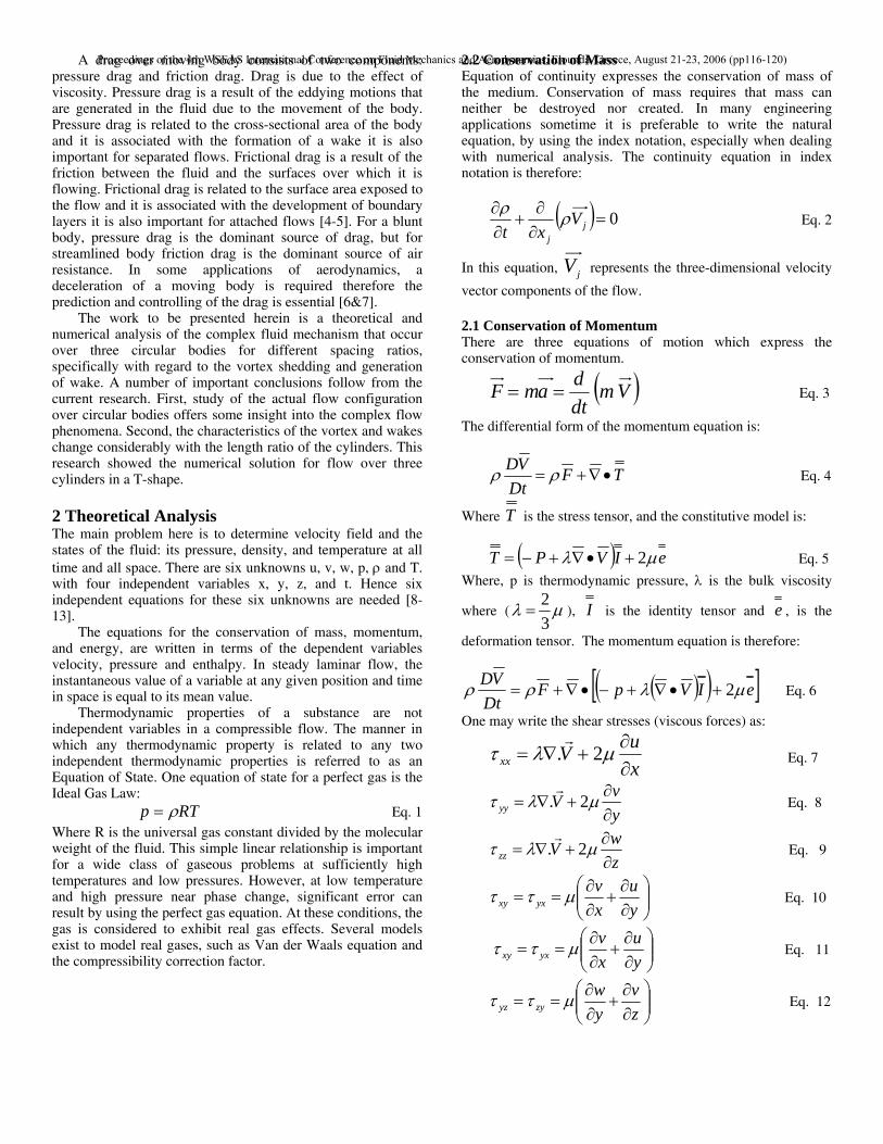
Theoretical and Numerical Study of Vortex-Wake Flow
Khaled Alhussan Research Assistant Professor, Space Research Institute, King Abdulaziz City for Science & Technology,
Saudi Arabia, P.O. Box 6086, Riyadh 11442
Abstract: - This paper is to show a numerical and theoretical analysis of vortex-wake generation for flow past three circular cylinders. The three cylinders are positioned in a T-shape and spaced at length ratios (s/r) from 2 to 8 and the Reynolds number range from 100 to 800. The numerical results show characteristics of the wakes changing considerably with the length ratios. This research showed the numerical solution for flow over three cylinders in a T-shape arrangement. From the numerical results, such as the path lines, one can conclude that the vortex generation and the wake region are affected by the spacing between the cylinders. For the length ratio of 2.0 one can see that the drag is minimized. Key- Words: Vortex, Karman vortex street, bluff body wake, numerical analysis.
Nomenclature Symbol Meaning
cv Specific heat at constant volume
e Internal energy
e Deformation Tensor
fij Viscous forces
I Identity tensor
ho Stagnation enthalpy
k Thermal conductivity
m Mass
p Static pressure
Q Heat generation
t Time
T Static temperature
T Stress tensor
U Mean velocity component
V Mean velocity component
W Mean velocity component
W Molecular Weight
εij Rate of strain tensor
γ Ratio of specific heat
δij Kronecker delta
ρ Density of fluid
λ Bulk viscosity
τij Shear stress
μ Coefficient of viscosity
1 Introduction Flow over external bodies has been studied extensively because of their many practical applications [1-3]. For example, flow past a circular cylinder, usually experiences strong flow oscillations and boundary layer separation in the wake region behind the body. As a fluid particle flows toward the leading edge of a cylinder, the pressure of the fluid particle increases from the free stream pressure to the stagnation pressure. The high fluid pressure near the leading edge of the cylinder forces flow about the cylinder as boundary layers develop about both sides.
The boundary layer separates from the surface forms a free shear layer and is highly unstable. This shear layer will eventually roll into a discrete vortex and detach from the surface. A periodic flow motion will develop in the wake as a result of boundary layer vortices being shed alternatively from either side of the cylinder. The periodic nature of the vortex shedding phenomenon can sometimes lead to unwanted structural vibrations, especially when the shedding frequency matches one of the resonant frequencies of the structure.
Vortices shed alternatively from the cylinder and generate a regular vortex pattern in the wake. This regular pattern of vortices in the wake is called Karman vortex street. It creates an oscillating flow at a discrete frequency that is correlated to the Reynolds number of the flow. Many numerical and experimental studies have focused on the dynamics of the bluff body wake and vortex street problems [4-6].
Proceedings of the 4th WSEAS International Conference on Fluid Mechanics and Aerodynamics, Elounda, Greece, August 21-23, 2006 (pp116-120)
A drag over moving body consists of two components: pressure drag and friction drag. Drag is due to the effect of viscosity. Pressure drag is a result of the eddying motions that are generated in the fluid due to the movement of the body. Pressure drag is related to the cross-sectional area of the body and it is associated with the formation of a wake it is also important for separated flows. Frictional drag is a result of the friction between the fluid and the surfaces over which it is flowing. Frictional drag is related to the surface area exposed to the flow and it is associated with the development of boundary layers it is also important for attached flows [4-5]. For a blunt body, pressure drag is the dominant source of drag, but for streamlined body friction drag is the dominant source of air resistance. In some applications of aerodynamics, a deceleration of a moving body is required therefore the prediction and controlling of the drag is essential [6&7].
The work to be presented herein is a theoretical and numerical analysis of the complex fluid mechanism that occur over three circular bodies for different spacing ratios, specifically with regard to the vortex shedding and generation of wake. A number of important conclusions follow from the current research. First, study of the actual flow configuration over circular bodies offers some insight into the complex flow phenomena. Second, the characteristics of the vortex and wakes change considerably with the length ratio of the cylinders. This research showed the numerical solution for flow over three cylinders in a T-shape. 2 Theoretical Analysis The main problem here is to determine velocity field and the states of the fluid: its pressure, density, and temperature at all time and all space. There are six unknowns u, v, w, p, ρ and T. with four independent variables x, y, z, and t. Hence six independent equations for these six unknowns are needed [8-13].
The equations for the conservation of mass, momentum, and energy, are written in terms of the dependent variables velocity, pressure and enthalpy. In steady laminar flow, the instantaneous value of a variable at any given position and time in space is equal to its mean value.
Thermodynamic properties of a substance are not independent variables in a compressible flow. The manner in which any thermodynamic property is related to any two independent thermodynamic properties is referred to as an Equation of State. One equation of state for a perfect gas is the Ideal Gas Law:
RTp ρ= Eq. 1
Where R is the universal gas constant divided by the molecular weight of the fluid. This simple linear relationship is important for a wide class of gaseous problems at sufficiently high temperatures and low pressures. However, at low temperature and high pressure near phase change, significant error can result by using the perfect gas equation. At these conditions, the gas is considered to exhibit real gas effects. Several models exist to model real gases, such as Van der Waals equation and the compressibility correction factor.
2.2 Conservation of Mass Equation of continuity expresses the conservation of mass of the medium. Conservation of mass requires that mass can neither be destroyed nor created. In many engineering applications sometime it is preferable to write the natural equation, by using the index notation, especially when dealing with numerical analysis. The continuity equation in index notation is therefore:
( ) 0=∂∂
+∂∂
jj
Vxt
ρρ Eq. 2
In this equation, jV represents the three-dimensional velocity
vector components of the flow. 2.1 Conservation of Momentum There are three equations of motion which express the conservation of momentum.
( )VmdtdamF == Eq. 3
The differential form of the momentum equation is:
TFDtVD
•∇+= ρρ Eq. 4
Where T is the stress tensor, and the constitutive model is:
( ) eIVPT μλ 2+•∇+−= Eq. 5
Where, p is thermodynamic pressure, λ is the bulk viscosity
where ( μλ32
= ), I is the identity tensor and e , is the
deformation tensor. The momentum equation is therefore:
( )( )[ ]eIVpFDtVD μλρρ 2+•∇+−•∇+= Eq. 6
One may write the shear stresses (viscous forces) as:
xuVxx ∂∂
+∇= μλτ 2.r
Eq. 7
yvVyy ∂∂
+∇= μλτ 2.r
Eq. 8
zwVzz ∂∂
+∇= μλτ 2.r
Eq. 9
⎟⎟⎠
⎞⎜⎜⎝
⎛∂∂
+∂∂
==yu
xv
yxxy μττ Eq. 10
⎟⎟⎠
⎞⎜⎜⎝
⎛∂∂
+∂∂
==yu
xv
yxxy μττ Eq. 11
⎟⎟⎠
⎞⎜⎜⎝
⎛∂∂
+∂∂
==zv
yw
zyyz μττ Eq. 12
Proceedings of the 4th WSEAS International Conference on Fluid Mechanics and Aerodynamics, Elounda, Greece, August 21-23, 2006 (pp116-120)
The x-momentum therefore is:
xzxyxxx fzyxx
pVutu ρτττρρ
+∂∂
+∂
∂+
∂∂
+∂∂
−=∇+∂
∂ ).()( r
Eq. 13 The y-momentum therefore is:
yzyyyxy fzyxy
pVvtv ρ
τττρρ
+∂
∂+
∂
∂+
∂
∂+
∂∂
−=∇+∂
∂ ).()( r
Eq. 14 The z-momentum therefore is:
zzzyzxz fzyxz
pVpwtw ρτττρ
+∂∂
+∂
∂+
∂∂
+∂∂
−=∇+∂
∂ ).()( r
Eq.15 The momentum equation can be written in tensor form where the shear stress tensor is used. The shear stress (viscous) tensor for Newtonian (linear fluid) therefore is:
Vxu
xu
iji
j
j
iij •∇+⎟
⎟⎠
⎞⎜⎜⎝
⎛
∂
∂+
∂∂
= λδμτ Eq. 16
Where ijδ is the kronecker delta and ijδ =1 for i=j and ijδ =0
for i≠j, the momentum equation in tensor form is:
( ) ij
ij
ij
i fxx
puux
ut ji ρ
τρρ +
∂
∂−
∂∂
−=⎟⎠⎞
⎜⎝⎛
∂∂
+∂∂ −−
Eq. 17 The three terms on the right-hand side of Eq. 17 represent the x-components of all forces due to the pressure, p, the viscous stress tensor,τij , and the body force, fi . 2.3 Conservation of Energy Equation The differential form of the energy equation is written in the same way as the continuity and the momentum equation, namely, by using Green’s theorem, hence:
( ) KQTVVFeVVDtD
•∇−+••∇+•=⎟⎟⎠
⎞⎜⎜⎝
⎛+
• ρρρ2
Eq. 18
Therefore the differential form of the total energy equation can be written in the following form, where the stress tensor is used and the assumption of the Newtonian fluid applied implicitly:
( ) ( ) ( ) ( ) ( )
( ) ( ) ( ) ( )
( ) ( ) ( ) Vfz
wy
wx
wz
vy
vx
vz
uy
ux
uz
wpyvp
xup
zTk
zyTk
yxTk
xQVe
DtD
zzyzxz
zyyyxyzx
yxxx
rr.
2
2
ρτττ
ττττ
ττ
ρρ
+∂
∂+
∂
∂+
∂∂
+
∂
∂+
∂
∂+
∂
∂+
∂∂
+
∂
∂+
∂∂
+∂
∂−
∂∂
−∂∂
−
⎟⎠⎞
⎜⎝⎛
∂∂
∂∂
+⎟⎟⎠
⎞⎜⎜⎝
⎛∂∂
∂∂
+⎟⎠⎞
⎜⎝⎛
∂∂
∂∂
+=⎟⎟⎠
⎞⎜⎜⎝
⎛+
Eq. 19 In some engineering applications, sometimes one wishes to deal with the internal energy alone or in another instance one may wish to evaluate the mechanism of transferring energy from one mode to another, such as in turbulent flow or in viscous situations therefore it will be helpful to develop the energy equation in terms of the internal energy alone. One way to derive the internal energy is to subtract the kinetic energy equation from the total energy equation.
The kinetic energy equation is obtained by using the dot product between two vectors namely the momentum equation and the velocity vector. Therefore the kinetic energy equation is:
( )zyx
zzyzxzzyyyxy
zxyxxx
wfvfufzyx
wzyx
v
zyxu
zpw
ypv
xpu
Dt
VD
+++
⎟⎟⎠
⎞⎜⎜⎝
⎛∂∂
+∂
∂+
∂∂
+⎟⎟⎠
⎞⎜⎜⎝
⎛∂
∂+
∂
∂+
∂
∂+
⎟⎟⎠
⎞⎜⎜⎝
⎛∂∂
+∂
∂+
∂∂
+∂∂
−∂∂
−∂∂
−=
ρ
ττττττ
τττρ 2
2
Eq. 20 One may subtract the kinetic energy obtained from dotting the velocity vector with the three directions of the momentum, therefore the internal energy equation may be written as:
⎥⎥⎥⎥⎥
⎦
⎤
⎢⎢⎢⎢⎢
⎣
⎡
⎟⎟⎠
⎞⎜⎜⎝
⎛∂∂
+∂∂
+⎟⎠⎞
⎜⎝⎛
∂∂
+∂∂
+
⎟⎟⎠
⎞⎜⎜⎝
⎛∂∂
+∂∂
+⎟⎠⎞
⎜⎝⎛∂∂
+⎟⎟⎠
⎞⎜⎜⎝
⎛∂∂
+⎟⎠⎞
⎜⎝⎛∂∂
+
⎟⎟⎠
⎞⎜⎜⎝
⎛∂∂
+∂∂
+∂∂
+⎟⎟⎠
⎞⎜⎜⎝
⎛∂∂
+∂∂
+∂∂
−
⎟⎠⎞
⎜⎝⎛
∂∂
∂∂
+⎟⎟⎠
⎞⎜⎜⎝
⎛∂∂
∂∂
+⎟⎠⎞
⎜⎝⎛
∂∂
∂∂
+=
22
2222
2
.
222
yw
zv
xw
zu
xv
yu
zw
yv
xu
zw
yv
xu
zw
yv
xup
zTk
zyTk
yxTk
xQp
DtDe
μ
λ
ρ
Eq. 21
Proceedings of the 4th WSEAS International Conference on Fluid Mechanics and Aerodynamics, Elounda, Greece, August 21-23, 2006 (pp116-120)
For incompressible fluid, , therefore, Tce v=
Qzw
yw
xw
zv
zyyv
yyxv
xyzu
zx
yu
xuTgradkdiv
DtDTc
zzyzxz
yxxx
ρτττ
ττττ
ττρ
+∂∂
+∂∂
+∂∂
+
∂∂
+∂∂
+∂∂
+∂∂
+
∂∂
+∂∂
+= )(
Eq. 22 For compressible fluid, therefore:
( ) ( ) ( )
( ) ( ) ( )
( ) ( ) ( )
Q
zw
yw
xw
zv
yv
xv
zu
yu
xu
tp
Tgradkdivuhdivth
zzyzxz
zyyyxy
zxyxxx
oo
ρ
τττ
τττ
τττ
ρρ
+
⎥⎥⎥⎥⎥⎥⎥⎥
⎦
⎤
⎢⎢⎢⎢⎢⎢⎢⎢
⎣
⎡
∂∂
+∂
∂+
∂∂
+
∂
∂+
∂
∂+
∂
∂+
∂∂
+∂
∂+
∂∂
+
∂∂
+=+∂
∂)()(
)(
Eq. 23 In tensor form the energy equation therefore is:
( ) ( ) ( ) iijjiij
oi
j
o fuQuxt
phux
ht
ρτρρ ++∂∂
−∂∂
=∂∂
+∂∂
Eq. 24
A numerical analysis must start with breaking the computational domain into discrete sub-domains, which is the grid generation process. A grid must be provided in terms of the spatial coordinates (x, y and z location) of grid nodes distributed throughout the computational domain. At each node in the domain, the numerical analysis will determine values for all dependent variables including pressure, velocity components and temperature.
Considering an infinitesimal control volume, the two terms on the left-hand side of this equation describe the rate of increase of ho and the rate at which ho is transported into and out of the control volume by convection. The first term on the right-hand side describes the influence of the pressure on the total enthalpy. The second term describes the rate at which work is done against viscous stresses by distortion of the fluid. The gradient of Q is the rate of energy transfer into the control volume by conduction, and the last term describes the rate of work done by body forces.
If the Navier-Stokes equations do not hold an equation of the stress tensor must be found and solved simultaneously with the four basic equations. Even when the Navier-Stokes relations hold, the relation of the coefficient of viscosity must be given with respect to the state variables of the fluid such as temperature and density.
There are many other cases where the basic equations of fluid dynamics are not sufficient or should be modified such as in the cases of the two-phase flow, multi-fluid flow theory, relativistic fluid mechanics and biomechanics.
3 Numerical Analysis Now, after stating all the flow equations, mass,
momentum, energy, and the constitutive laws that govern the transport relations, it is time to formulate a solution. But, since, these equations are coupled nonlinear, partial differential equations, it is impossible to have a closed form of solution. In
order to formulate or approximate a valid solution for these equations they must be solved using computational fluid dynamics technique. In order to solve these equations numerically with a computer, they must be discretized. That is, the continuous control volume equations must be applied to each discrete control volume that is formed by the computational grid. The integral equations are substituted with a set of linear algebraic equations solved at a discrete set of points.
In a finite element discretization the grid breaks up the domain into elements over which the changes of the fluid variables are evaluated. Adding all the variations for each element then gives an overall visualization of how the variables vary over the entire domain. The primary advantage of the finite element method is the geometric flexibility allowed by a finite element grid. In a finite volume discretization the grid breaks up the domain into nodes, each associated with a discrete control volume. The fluxes of mass, momentum, and energy for each control volume are then calculated at each node. An advantage of the finite volume method is that the principles of mass, momentum, and energy conservation are applied directly to each control volume, so that the integral conservation of quantities is exactly satisfied for any set of control volumes in the domain. Thus, even for a coarse grid, there is an exact integral flux balance [8].
The nodes must be distributed throughout the volume enclosed by the exterior boundary surface of the domain such that they form a complete three-dimensional matrix of nodes. Each node in the matrix will be referred to by the index triplet (i, j, k).
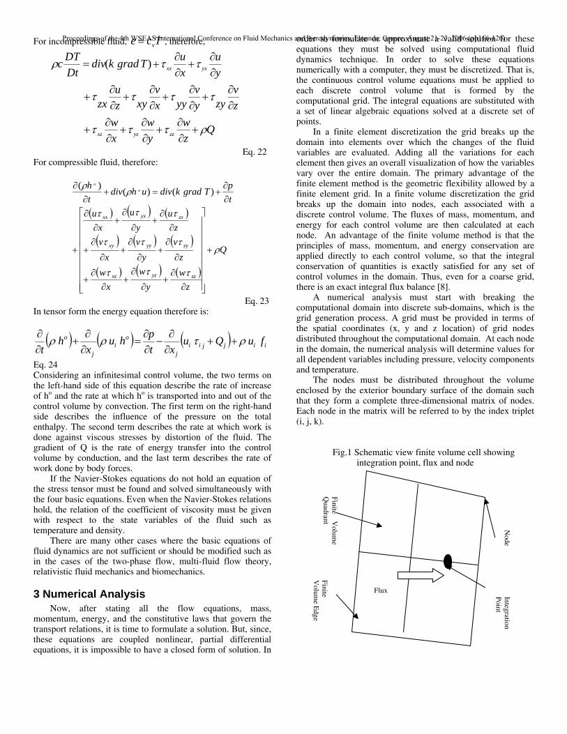
Fig.1 Schematic view finite volume cell showing integration point, flux and node
Finite
Volum
e Q
uadrant
Finite V
olume E
dge
Integration Point
Node
Flux
Proceedings of the 4th WSEAS International Conference on Fluid Mechanics and Aerodynamics, Elounda, Greece, August 21-23, 2006 (pp116-120)

3.1 Flux Elements To complete the description of the distribution of nodes in the computational domain, it is useful to introduce the concept of a flux element. A flux element, such as shown in Figure 1, is a linear, hexahedral element defined by eight nodes. Conforming to the finite element approach, linear shape functions representing the variation of variables within the flux element are applied [8]. Each flux element has four octants for two-dimensional domain and eight octants for three-dimension region. The six sides of each octant are divided into two groups; those that are coincident with the flux element sides and those that are in the interior of the flux element. Because the latter group will form the surfaces of the control volume over which surface integrals will be evaluated, they are referred to as, integration point surfaces, as shown in Figure 1. 3.2 Control Volumes In finite volume method a control volume exists for each node, with the boundary of each interior control volume defined by eight line-segments in two dimensions and 24 quadrilateral surfaces in three dimensions. To solve the governing or the natural equations that were derived in theoretical section they must be converted to their discrete or algebraic form. 3.3 Discretization Discretization is the process whereby the governing equations are converted by their discrete form. Discretization identifies the node locations and flux elements to model the flow problem. The differential equations are transformed to algebraic equations, which should correctly approximate the transport properties of the physical processes.
Next, the fluxes are evaluated at integration points, which are shared by adjacent control volumes. The same flux that leaves one control volume enters the next one. Thus, even with a low accuracy advection scheme numerical conservation is guaranteed. This is the fundamental advantage of a finite volume method. The discretization is evaluated in an elemental basis [8]. 4 Results and Discussion Figure 2 shows a schematic view of the three circular cylinders that are placed in T-Shape configuration. The length S is the distance between the leading circular cylinder and the centers of the aligned two cylinders. The length ratio is defined as the s/r, where r is the radius of the cylinder. The length ratio is varied from 2.0 to 8.0, for a range of Reynolds number from 100 to 800. From the numerical solution one can study the characteristics of the vortex changing and wake generation for cross flow past three circular cylinders. This paper shows details of the vortex interference in the wake region of three circular cylinders. Many researchers have studied variation of vortex generation according to the spacing between two cylinders in tandem arrangement [14 & 15]. Drag and vortex mode shape change across critical spacing [16]. There is a drastic change in vortex mode at critical spacing of about 3.5 to 4 [17]. Vortex wake pattern depend on whether or not there exist vortex shedding between the cylinders [14-17].
Fig.2 Schematic view of three circular cylinders
showing the boundary conditions for the numerical simulations
S
Static Pressure
Inlet-Outlet Pressure
Total Pressure
Inlet-Outlet Pressure
Figure 3 shows path lines for flow past three circular cylinders, the length ratio is 2.0. One can see the vortex generation and the wake region generated by the leading cylinder. One can conclude from this figure that the wake region generated by the leading cylinder is minimized by the present of the other two cylinders. The vortices that are generated at the aligned cylinders are affected by the wake of the leading cylinder and this has an influence in reducing vortex shedding of the aligned cylinders.
The path lines for flow past three circular cylinders of length ratio of 4.0 are show in figure 4. One can notice that the wake region of the leading cylinder is grater than the one shown in figure 3. Figure 5 shows the path line for length ratio of 8.0, where one can see that the leading cylinder has little effect on the other two cylinders.
Fig.3 Path lines for flow past three circular cylinders (s/r=2.0)
Proceedings of the 4th WSEAS International Conference on Fluid Mechanics and Aerodynamics, Elounda, Greece, August 21-23, 2006 (pp116-120)
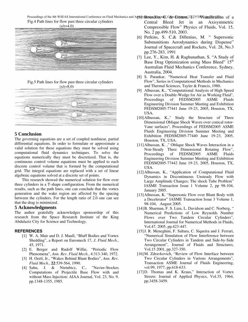
Fig.4 Path lines for flow past three circular cylinders
(s/r=4.0)
Fig.5 Path lines for flow past three circular cylinders (s/r=8.0)
5 Conclusion The governing equations are a set of coupled nonlinear, partial differential equations. In order to formulate or approximate a valid solution for these equations they must be solved using computational fluid dynamics techniques. To solve the equations numerically they must be discretized. That is, the continuous control volume equations must be applied to each discrete control volume that is formed by the computational grid. The integral equations are replaced with a set of linear algebraic equations solved at a discrete set of points.
This research showed the numerical solution for flow over three cylinders in a T-shape configuration. From the numerical results, such as the path lines, one can conclude that the vortex generation and the wake region are affected by the spacing between the cylinders. For the length ratio of 2.0 one can see that the drag is minimized. 5 Acknowledgments The author gratefully acknowledges sponsorship of this research from the Space Research Institute of the King Abdulaziz City for Science and Technology.
REFERENCES [1] W. A. Mair and D. J. Maull, “Bluff Bodies and Vortex
Shedding”, a Report on Euromech 17, J. Fluid Mech., 45, 1971.
[2] E. Berger and Rudolf Willie, “Periodic Flow Phenomena”, Ann. Rev. Fluid Mech., 4:313-340, 1972.
[3] H. Oertl, Jr., “Wakes Behind Blunt Bodies”, Ann. Rev. Fluid Mech., 22:539-564, 1990.
[4] Sahu, J. & Nietubicz, C., ”Navier-Stockes Computations of Projectile Base Flow with and without Mass Injection: AIAA Journal, Vol. 23, No. 9, pp.1348-1355, 1985.
[5] Bourdon, C. & Dutton, J. “ Visualization of a Central Bleed Jet in an Axisymmetric Compressible Flow” Physics of Fluids, Vol. 15, No. 2 pp.499-510, 2003.
[6] Perkins, S. C.& Dillenius, M. “ Supersonic Submunitions Aerodynamics during Dispense” Journal of Spacecraft and Rockets, Vol. 28, No.3 pp.276-283, 1991
[7] Lee, Y., Kim, H. & Raghunathan, S. “A Study of Base Drag Optimization using Mass Bleed” 15th Australian Fluid Mechanics Conference, Sydney, Australia, 2004.
[8] S. Patankar, “Numerical Heat Transfer and Fluid Flow”, Series in Computational Methods in Mechanics and Thermal Sciences, Tayler & Francis, 1980.
[9] Alhussan, K., “Computational Analysis of High Speed Flow over a Double-Wedge for Air as Working Fluid", Proceedings of FEDSM2005 ASME Fluids Engineering Division Summer Meeting and Exhibition FEDSM2005-77441 June 19-23, 2005, Houston, TX, USA.
[10] Alhussan, K.," Study the Structure of Three Dimensional Oblique Shock Waves over conical rotor-Vane surfaces", Proceedings of FEDSM2005 ASME Fluids Engineering Division Summer Meeting and Exhibition FEDSM2005-77440 June 19-23, 2005, Houston, TX, USA.
[11] Alhussan, K. ," Oblique Shock Waves Interaction in a Non-Steady Three Dimensional Rotating Flow", Proceedings of FEDSM2005 ASME Fluids Engineering Division Summer Meeting and Exhibition FEDSM2005-77442 June 19-23, 2005, Houston, TX, USA.
[12] Alhussan, K., “Application of Computational Fluid Dynamics in Discontinuous Unsteady Flow with Large Amplitude Changes; The shock Tube Problem” IASME Transaction Issue 1 Volume 2, pp 98-104, January 2005.
[13] Alhussan, K. “Supersonic Flow over Blunt Body with a Decelerator” IASME Transaction Issue 3 Volume 1, 98-104, August 2005.
[14] B. Sharman, F. S. Lien, L. Davidson and C. Norberg, “ Numerical Predictions of Low Reynolds Number Flows over Two Tandem Circular Cylinders”, International Journal for Numerical Methods in Fluids, Vol.47, 2005, pp.423-447.
[15] J. R. Meneghini, F. Saltara, C. Siqueira and J. Ferrari, “Numerical Simulation of Flow Interference between Two Circular Cylinders in Tandem and Side-by-Side Arrangement”, Journal of Fluids and Structures, Vol.15 2001, pp.327-350.
[16] M. Zdravkovich, “Review of Flow Interface between Two Circular Cylinders in Various Arrangements”, Transaction ASME Journal of Fluids Engineering, vol.99, 1977, pp.618-633.
[17] D. Thomas and K. Kraus,” Interaction of Vortex Streets: Journal of Applied Physics, Vol.35, 1964, pp.3458-3459.
Proceedings of the 4th WSEAS International Conference on Fluid Mechanics and Aerodynamics, Elounda, Greece, August 21-23, 2006 (pp116-120)