1

Theory of Gelation

Post-Gelation Behavior

Kazumi Suematsu

Institute of Mathematical Science

Ohkadai 2-31-9, Yokkaichi, Mie 512-1216, JAPAN

Fax: +81 (0) 593 26 8052, E-mail address: suematsu@m3.cty-net.ne.jp

2

Summary

Within the framework of the random distribution assumption of cyclic bonds, the preceding

theory of gelation is extended to mixing systems with various functionalities. To examine the

validity of the assumption, the theory is applied to experimental data in polyurethane network

formation, the result showing the soundness of the theory for the prediction of gel points and gel

fraction.

Key Words

Gel Point/ Cyclization/ Mixing System/ Critical Dilution/ Gel Fraction/

3

1. Introduction

There remain some unsolved problems in polymer science. Of those, the determination of the

gel point of branched polymer solutions has been one of the most attracting subjects for more than

60 years. It has been shown that the gel point varies widely from systems to systems, often deviating

markedly from the ideal values [1]. It was pointed out earlier that the discrepancy between the

theoretical point and observed ones can be ascribed to the neglect of cyclization [2]. Based on the

findings of the early researchers, the author has pursued so far the general theory of gelation that

includes cyclization effects [3].

In this report, the author will extend the preceding theory to mixing systems. The essence of our

approach is based on the following four premises (three principles and one assumption):

Three Principles

(i) The gel point is divided into the two terms:

D D inter D ringc . (1)

(ii) The total ring concentration, [], is independent of the initial monomer concentration, C; it

is a function of D (the extent of reaction) alone.

(iii) Branched molecules behave ideally at C .

One Assumption

(iv) Assumption I: Cyclic bonds distribute randomly over all bonds.

The premise (i) is a mathematical theorem. The premise (ii) is based on the following formal

solution of []:

C dDR L

R LDj

jv v

v v11, (2)

which is common to all model systems, where vR j denotes the velocity of j-ring formation and

v vR Rj j

, and vL that of intermolecular reaction. Experiments have shown that the relative

velocity, v vR Lj, is a decreasing function of the initial monomer concentration, C, which implies

that eq. (2) is of the form: C t dD1 1 , a function rapidly approaching a constant with

increasing t (t is a representation of the concentration of reactants). This tells us that [] is constant

at high concentration, which, in fact, has been verified rigorously for f 2 [3]. The premise (iii)

can not be verified immediately by experimental methods, but has solid physical foundation: (a)

experiments have shown that v vR Lj 0 as C large , so that the production of rings becomes

negligible at high concentration; (b) all excluded volume effects vanish rigorously at C [3],

[4], since, as C , the monomer density becomes infinite and the notion of atomic radii vanishes.

In contrast to the above three principles, the premise (iv) (Assumption I) is an approximation.

Assumption I, however, greatly simplifies the problem. It reduces otherwise an inherently insoluble

problem of gelation to an elementary mathematical exercise, giving the equality D inter Dco .

4

Eq. (1) then becomes

D D pc co R , (3)

with Dco being the Flory point, and pR the fraction of cyclic bonds to all possible bonds and can be

equated with D ring [3].

In this report, the author generalizes, within the framework of the above three principles and one

assumption, the preceding theory to include mixing systems of multifunctionalities.

2. Theoretical

2-1) R-Af Model

Gel Point

Suppose that a reaction system is comprised of a mixture, f Mi i , of branching units, with fi

being the functionality and Mi the mole number. Let Χ i i i i iif M f M be the fraction of functional

units (FU’s) belonging to the ith branching unit. Let D be the extent of reaction of all FU’s, J be the

number of FU’s to form a junction point. Let X and Z be sets of all bonds and cyclic bonds,

respectively. Each ring possesses only one excess (cyclic) bond. Under Assumption I, the probability,

Α , that a branching unit leads to the next branching unit to form a network is equal to the product

of the fraction of reacted functional units and the fraction of intermolecular bonds. Hence

Α Χ

ii

i k f k

k

fJ

J

kf

kD D J P Z X P Z Xi

i 1 1 1 11

0

11

0

1

ll

l l

l

| | . (4)

where P Z X P Z X P X| is the conditional probability that a randomly chosen bond is a

cyclic bond. Thus the quantity, 1 P Z X| , represents the probability that a chosen bond is an

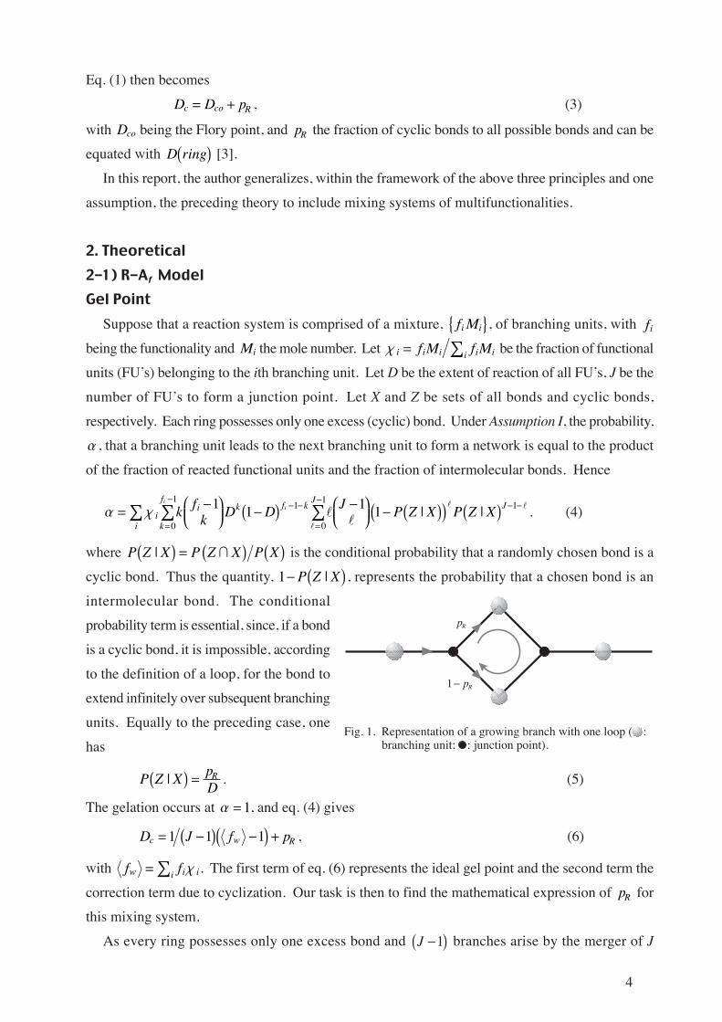
intermolecular bond. The conditional

probability term is essential, since, if a bond

is a cyclic bond, it is impossible, according

to the definition of a loop, for the bond to

extend infinitely over subsequent branching

units. Equally to the preceding case, one

has

P Z X

pDR| . (5)

The gelation occurs at Α 1, and eq. (4) gives

D J f pc w R 1 1 1 , (6)

with f fw ii i Χ . The first term of eq. (6) represents the ideal gel point and the second term the

correction term due to cyclization. Our task is then to find the mathematical expression of pR for

this mixing system.

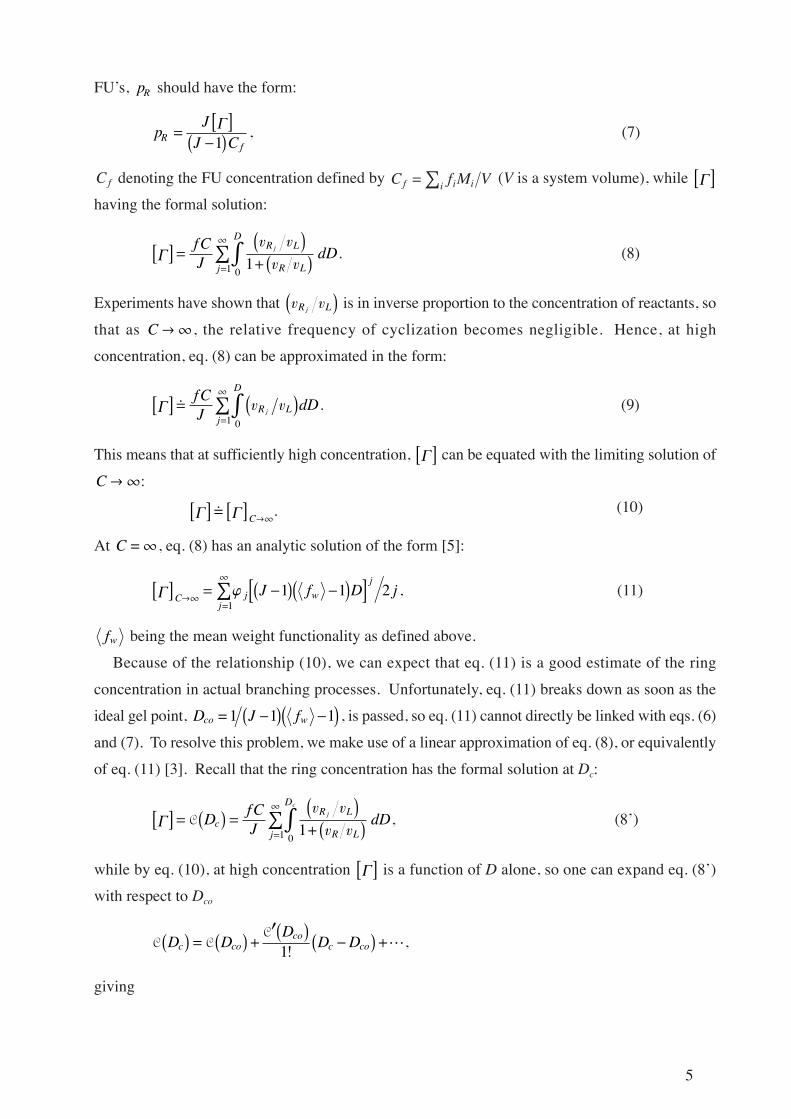
As every ring possesses only one excess bond and J 1 branches arise by the merger of J

pR

1 pR

Fig. 1. Representation of a growing branch with one loop ( :branching unit; : junction point).

5

FU’s, pR should have the form:

p

JJ CR

f

1

, (7)

Cf denoting the FU concentration defined by C f M Vf i ii (V is a system volume), while having the formal solution:

f CJ

dDR L

R L

D

j

jv v

v v101

. (8)

Experiments have shown that v vR Lj is in inverse proportion to the concentration of reactants, so

that as C , the relative frequency of cyclization becomes negligible. Hence, at high

concentration, eq. (8) can be approximated in the form:

f CJ

dDR L

D

jj

v v01

. (9)

This means that at sufficiently high concentration, can be equated with the limiting solution of

C :

C. (10)

At C , eq. (8) has an analytic solution of the form [5]:

C j w

j

jJ f D j 1 1 2

1, (11)

fw being the mean weight functionality as defined above.

Because of the relationship (10), we can expect that eq. (11) is a good estimate of the ring

concentration in actual branching processes. Unfortunately, eq. (11) breaks down as soon as the

ideal gel point, D J fco w 1 1 1 , is passed, so eq. (11) cannot directly be linked with eqs. (6)

and (7). To resolve this problem, we make use of a linear approximation of eq. (8), or equivalently

of eq. (11) [3]. Recall that the ring concentration has the formal solution at Dc:

C Df CJ

dDcR L

R L

D

j

j

c v v

v v101

, (8’)

while by eq. (10), at high concentration is a function of D alone, so one can expand eq. (8’)

with respect to Dco

C C

CD D

DD Dc co

coc co

1!L,

giving

6

jj

wj

jc coj

J fD D2

1 12

, (12)

which, now, can be applied to the new territory, D D Dco c . Eq. (12) has sound mathematical

basis because of the relationship of eq. (10). From eqs. (6), (7) and (12), one has

DJ f

jc

w

J fj fj

J fj fj

w

w

!

"

#

$

11 1

1 1 1

1

1

2

1

2

/ Γ

Γ, (13)

where Γ f fC1 is the reciprocal of the initial FU concentration. For a single component system,

f fw and Γ Γf f , and one recovers the preceding result. Thus eq. (13) is an extension of the

previous expression.

Post-gelation

We confine ourselves to a mixture of monomers with f &2. Let Q be the probability that a

chosen branch emanating from a monomer is finite [6]-[8]. Following the aforementioned

Assumption I, Q satisfies the recurrence relation:

Q D D

pD

pD

QiR R f

i

J

i

!

"#

$

1 1 11

Χ . (14)

It is easy to show that eq. (14) has two solutions, Q1 and

D p Q Q X XR i

f f

i

J Ji i Χ 2 3 2 31 1 1L L , (15)

with

X

pD

pD

QiR R f

ii

Χ 1 1 .

The assignment of branching units can be made by the binomial expansion:

Ω Ωi

f

ii

i f i f

iQ Q

fQ Q

fQ Qi i i1 0 1 1 10 1 1

! "#

$

L , (16)

with Ω Χ

Χim M

m Mm f

m fi i

i ii

i i i

i i ii

being the weight fraction of the ith monomer unit and mi the molecular

mass. The first term of eq. (16) represents the weight fraction (ws) of sol, the second term the

fraction (wp) of pendants, and the higher terms than the third the fraction of active network segments.

Hence

w w Qs g i

f

i

i 1 Ω , (17)

w

fQ Qp i

i f

i

i

Ω 1 1 1 1 . (18)

7

To calculate the post-gelation behavior, we extend the concept of cyclization in sol phase to gel

phase; namely, we apply the foregoing linear approximation shown in eq. (12) to the gel phase and

write

jj

wj

jcoj

J fD D2

1 12

, (19)

for D Dco 1. In this expression, it is assumed that all reactions are smooth and continuous

beyond the gel point with no reaction anomaly. Substitution of eq. (19) into eq. (17), with the help

of eqs. (7) and (15), gives a solution of wg as functions of D, Κ and Γf .

Q 1, Critical Case

Set Q1 and eq. (15) gives the critical condition, D J f pc w R 1 1 1 , in agreement

with eq. (6).

2-2) R-Ag + R-Bf-g Model

Gel Point

Let there be a mixing system comprising of two different types of monomer units, g Mi Ai and

f g M

j B j , where MAi

and MB j are the mole numbers of the A type and the B type monomers,

respectively, and gi and

f gj

are the corresponding functionalities. Let J be the total number of

FU’s to form a junction point on which the two types of the FU’s are arranged alternately. By the

nature of the R A R B g f g model, J must be an even integer and J1 branches arise as a

result of the merger of J 2 A type FU’s and J 2B type FU’s. Thus, the probability, Α, of branching

becomes

Α

!

"#

$

D P Z X g P Z X f g D s P Z X gAJ

AA wJ

AB w Bi J

AB wi

2 2 20

1 1 1 1 1 1 1| | |

(20)

where s P Z X f g DJ

BB w B 2 1 1 1| , the subscripts, AA, AB and BB denote cyclic

formation via respective bond species, and the subscript, w, inside the bracket L the weight

average quantity. For Α 1, eq. (20) gives the gelation condition:

D P Z X gP Z X g f g D

P Z X f g DA

JAA w

JAB w w B

JBB w B

22

2 2

2

1 1 11 1 1

1 1 1 11

!

"

#

$ |

|

|.

(21)

Unfortunately, the solution is much intricate and difficult to use. So, here we examine the J 2

case only, for which eq. (21) reduces to

g f g P Z X D Dw w AB A B 1 1 1 1

2| . (21’)

Substituting P Z X p DAB R A| into eq. (21’), we have the critical condition:

8

D g f g pc w w R Κ 1 1 , (22)

with Dc representing the extent of reaction of A FU’s. Eq. (22) is the R A R B g f g model

version of eq. (6). Since pR is the ratio of cyclic bonds to all possible bonds, it may be written in

the form:

p

CRf A

f

,1 Κ Γ , (23)

with C g M Vf A i Ai i, being the concentration of A FU’s, Κ f g M g M

j Bj i Aij i, the

molar ratio of B FU’s to A FU’s (we define Κ &1), and

Γ f i A j BjiV g M f g M

i j , (24)

the reciprocal of the total FU concentration.

pR as a function of Dc can be obtained in the same manner as in eq. (12). We write

C dDf AR L

R L

D

j

j

c

,v v

v v101

, (25)

for which eq. (25) has the asymptotic solution of C :

C j w w

j

jg f g D j Κ1 1 22

1

. (26)

With the relationship, C , at high concentration in mind, expand eq. (25) with respect to

D Dco and substitute into eq. (23) to get

p jD

D DR jj co

j c coj

f

! "#

$

1 2 11 1

Κ Γ . (27)

Substituting eq. (27) into eq. (22), we have the gel point expression for the mixing system of the

R A R B g f g model J 2 :

D Dj

c coj fj

j fj

!

"#

$

1 1 1 2

1

K

K

Γ

Γ. (28)

Here K 1 Κ Dco and D g f gco w w

Κ 1 1 . Eq. (28) just corresponds to the

following transformation of the homogeneous system [3]:

Γ Γ f ;

functionality weight average functionality .

Post-gelation J = 2 We consider the mixture of f &2 monomers. Let QA be the probability that a branch emanating

from an A type monomer unit is finite, and QB the corresponding probability for a B type unit.

9

Then QA and QB satisfy

Q D D

pD

pD

QA A A B jR

A

R

AB

f g

j

j

1 1 1Χ ;

Q D D

pD

pD

QB B B AiR

A

R

AA

g

i

i

1 1 1Χ , (29)

with ΧAi i A i Aig M g Mi i

and Χ Bj j B j Bj

f g M f g Mj j

. The binomial expansion of

the probabilities, Q, is

Ω Ω ΩA A A

g

iB B B

f g

jA

iAg i

A Ag

ii

i

j

j

i

i iQ Q Q Qg

Qg

Q Q1 10 1

1 1

!

"#

$

L

ΩB

jB

f g jB B

f g

jj

j jf g

Qf g

Q Q

!

"#

$

0 11

1L . (30)

The respective first terms represent the weight fraction of sol:

w w Q Qs g A A

g

iB B

f g

ji

i

j

j 1 Ω Ω , (31)

where ΩAi and ΩB j

are the weight fractions of the ith A type and the jth B type monomer units,

respectively.

Special Solution I

Let us consider a mixing system of gi 2 (for all i s), f g 12, f g

23 and J 2.

This special system has an application to the polyurethane network formation of MDI (4,4’-

diphenylmethane diisocyanate: mA 250) and LHT240 (polyoxypropylene triol: mB 708).

LHT240 is considered to be a mixture of diols and triols [9]:

There are conflicting views about chemical constituents of LHT240. Adam and coworkers [10]

report that LHT240 is purely trifunctional, while Ilavsky and coworkers [9] report that it is a mixture

of diols and triols. The difference of the views stems from the difference in the characterization of

LHT240, especially in the estimation of OH content (see Table 1). Although which estimation is

Table 1. Chemical characterization of LHT240

Adam et al [10] Ilavsky et al [9]

Calculated Functionality

Number Average MW 715 by SEC 708 by VPO

OH Content (w/w %) 7.14 6.94

f - g = 3

f - g( )n= 2.89

SEC: Size exclusion chromatographyVPO: Vapour pressure osmometry

10

correct is indecisive at present, we use here the Ilavsky and coworkers estimation, since then the

theory can reasonably explain all the observed points.

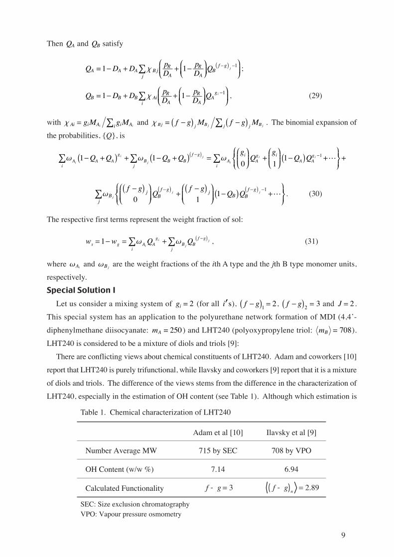
Let ΧB2 be the mole fraction of the triols to the total alcohols as defined above. Eq. (29) yields

Q

D p

D pA

B R

B R

=11 2

2

23

Κ Κ Χ

Χ, Q

D p

D pB

R

B R

=Κ

Χ

2

22 . (32)

Substituting into eq. (31), one has the weight fraction of gel:

w Q Q Qg A A B B B B 1 21

22

3Ω Ω Ω . (33)

In Figs. (2) and (3), eq. (33) is plotted as a function of

Γ f and Κ at D1, respectively. The parameters

employed here are those [3] of MDI-LHT240 (see Table

2). The relative cyclization frequency, j , the only

unknown parameter, is evaluated, based on the premise

(iii), by the equation:

Π Νj d dA

d d ddN

mole l 2 2 2 2 2/ , /

l , (34)

where d is dimension, l is the standard bond length

which can be equated with the C-N bond length

( 1 36. Ao

), d d2 2, Ν is the incomplete Gamma function,

and Ν is the proportionality factor defined by

r C jj F

2 2 2

+ Ν Ξl l , with CF being the Flory

characteristic constant in the + state and Ξ the effective

bond number per a repeating unit of the polymer

backbone [3].

The weight fractions, Ω, can be calculated using

the molecular weights, m, of respective branching

Table 2. Chemical constants of MDI-LHT240 mixture [3]

Functionality g = 2, f - g( )n= 2.89, f - g( )w

= 2.92, c B2 = 0.92

Mean Molecular Mass mA = 250 MDI( ), mB = 708 LHT240( )Flory Characteristic Constant CF = 4.5

Standard Bond Length l = 1.36 Ao

Effective Bond Number x = 68

Relative Frequency j j 2 jj=1

¶

Ê = 0.0272, j jj=1

¶

Ê = 0.1056

Fig. 2. wg vs Γ f curves of the MDI-LHT240 mix-ture (D 1).Solid line: theoretical line by eq. (33); (Κ 1 0. ), (Κ 1 3. ), and × (Κ 1 5. ):experimental points by Ilavsky and Dusek; : theoretical points by the ideal tree theory.

Γ f is a function of Κ itself and was calculatedby the formula:

ΓΚ

Ρ Κf

n A n n B n

n n

f g m g m

g f g

, ,

1000 1v l mol ,where the subscript n denotes the numberaverage, Ρ is the density of the polymericmaterials and v the volume fraction.

0 1 2 2.5

g f

0.0

0.2

0.4

0.6

0.8

1.0

wg

k =1.0

k =1.3

k =1.5

11

units. For the diols ( mB1) and the triols ( mB2) in

question, the observed heterogeneity index,

m mw n 1 03. [10] provides two possible solutions,

m mB B1 2, 359, 751 , 1057, 665 .Not surprisingly, graphical examination showed that

these two solutions gave almost identical wg Κ curves

when applied to eq. (33). For this reason, we mention

o n l y t h e r e s u l t f o r t h e s o l u t i o n ,

m m mA B B, ,1 2 250 ,1057, 665 .The solid lines in Fig. 2 show the theoretical ones;

the symbols ( : Κ 1 0. ; : Κ 1 3. ; × : Κ 1 5. )

are the experimental points by Ilavsky and Dusek [9];

the open circles () represent the theoretical values

predicted by the ideal tree theory Γ f 0 with no rings

and no excluded volume effects. By the aforementioned

reasons (Section I), we expect that all the data should

converge on these limiting cases (), as Γ f 0. Both

the theory and the experiments show that wg is less than

unity at D1, suggesting that the permanent sol

discussed precedently [3] is produced more abundantly

with increasing Γ f .

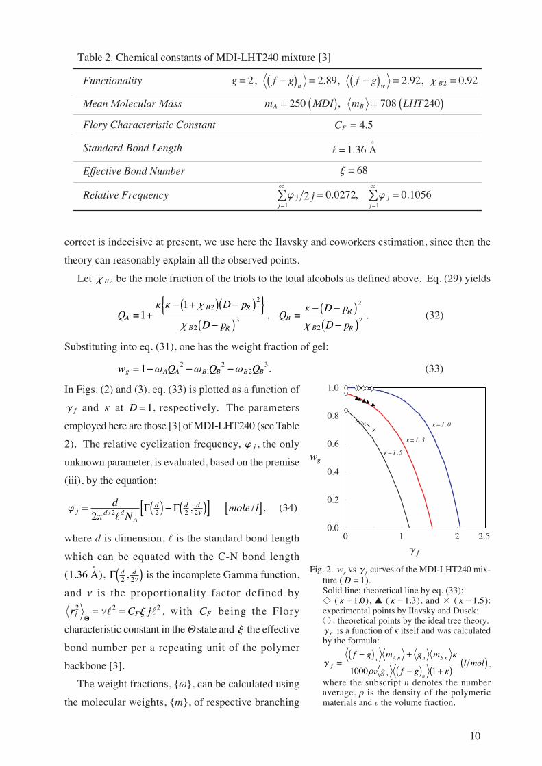
Fig. 3 shows the Κ dependence of wg . The solid

line is the theoretical one calculated by eq. (33), and

the broken line is the ideal case of pR 0; open circles

() are observed points. Agreement between the

theory and the experiments is satisfactory.

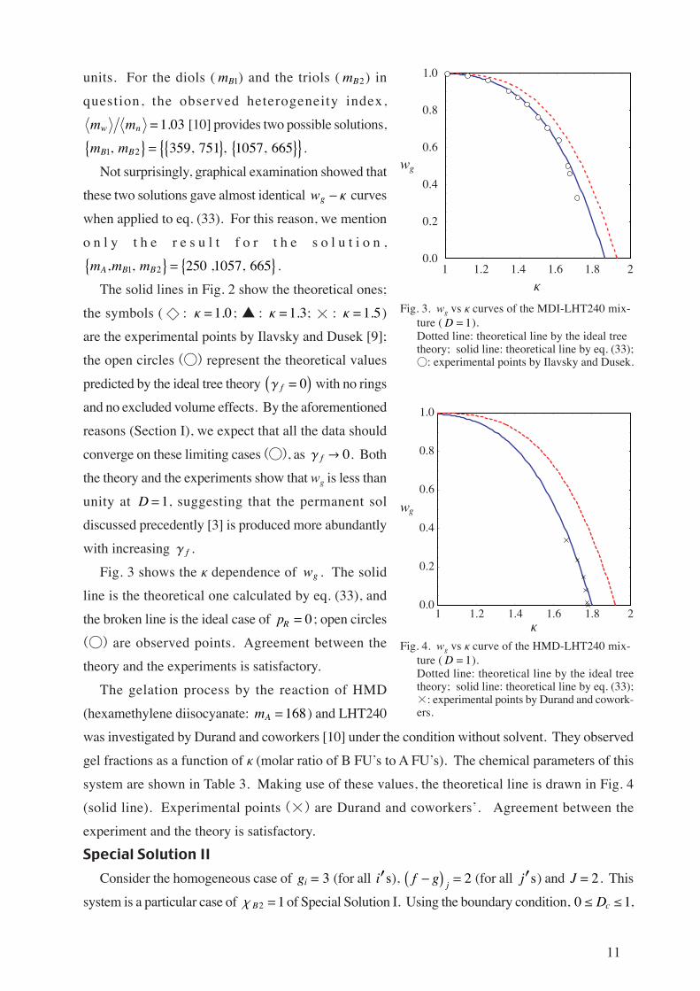
The gelation process by the reaction of HMD

(hexamethylene diisocyanate: mA 168) and LHT240

was investigated by Durand and coworkers [10] under the condition without solvent. They observed

gel fractions as a function of Κ (molar ratio of B FU’s to A FU’s). The chemical parameters of this

system are shown in Table 3. Making use of these values, the theoretical line is drawn in Fig. 4

(solid line). Experimental points (×) are Durand and coworkers’. Agreement between the

experiment and the theory is satisfactory.

Special Solution II

Consider the homogeneous case of gi 3 (for all i s),

f gj

2 (for all j s) and J 2. This

system is a particular case of ΧB2 1 of Special Solution I. Using the boundary condition, 0 1 Dc ,

Fig. 3. wg vs Κ curves of the MDI-LHT240 mix-ture (D 1).Dotted line: theoretical line by the ideal treetheory; solid line: theoretical line by eq. (33);: experimental points by Ilavsky and Dusek.

1 1.2 1.4 1.6 1.8 2

k

0.0

0.2

0.4

0.6

0.8

1.0

wg

Fig. 4. wg vs Κ curve of the HMD-LHT240 mix-ture (D 1).Dotted line: theoretical line by the ideal treetheory; solid line: theoretical line by eq. (33);×: experimental points by Durand and cowork-ers.

1 1.2 1.4 1.6 1.8 2k

0.0

0.2

0.4

0.6

0.8

1.0

wg

12

eq. (28) gives the critical-dilution condition:

Γ ΓΚ

f f cco

co jj

DD j

,1

1 1 1 1 2, (35)

with Dco Κ 2 . In order for the gelation to occur, Γ f must be less than the above critical value,

Γ f c, . The weight fraction of gel is given by

wD p

D p D pg A

R

R

B

R

!

"

#

$

!

"#

$

12 2

3

2

2

3

ΩΚ Κ

ΩΚ

1 1 . (36)

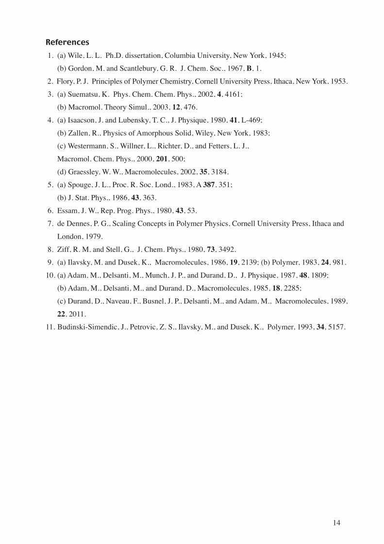
Eq. (35) is applied to Budinski-Simendic and coworkers’ experiments [11] for the polyurethane

network made from TI (tris-4-isocyanatophenylthiophosphate: mA 465 ) and PD

(polyoxypropylenediol: mB 970). With the help of the parameters in Table 4, eq. (35) can be

plotted as a function of Κ(solid line; Fig. 5 & Fig. 6). The symbols () denote the experimental

points by Budinski-Simendic and coworkers. Agreement between the theory and the observations

is excellent. It is important to notice that the classical tree theory (broken line) cannot explain these

Table 4. Chemical constants of TI-PD mixture [11]

Functionality g = 3, f - g = 2

Mean Molecular Mass mA = 465 TI( ) , mB = 970 PD( )Flory Characteristic Constant CF = 4.3

Standard Bond Length l = 1.36 Ao

Effective Bond Number x = 98

Relative Frequency j j 2 jj=1

¶

Ê = 0.0169, j jj=1

¶

Ê = 0.0680

j j 2 jj=1

¶

Ê = 0.0583 j jj=1

¶

Ê = 0.2267,

Table 3 Chemical constants of HMD-LHT240 mixture

13

observed values.

In Fig. 7, eq. (36) is plotted as a function of D: the

solid line __ corresponds to v1 and the broken line

v 0 2. (v denotes the volume fraction of

polymer). The dotted line L shows the ideal tree

theory with no rings. To date, within our knowledge,

there are no experimental observations corresponding

to the dilution regime of v 0 2. .

The results of Figs. (3)-(6) support the soundness of

the theory. We must bear in mind, however, that

Assumption I is an approximation. The experimental

determination of gel points is a difficult task, so

theoretical errors may be hidden behind experimental

errors. For this reason, it will be necessary to scrutinize

further the validity of Assumption I by extensive

experimental observations.

4. Conclusion

The theory of gelation was applied to the observed data in polyurethane networks. Good

agreement was found between the theory and the observations, both in the predictions of gel points

and gel fractions.

Fig. 6. Γf dependence of Κc for the TI-PD mixture.Dotted line: prediction of the ideal tree theory;solid line: prediction of eq. (35); : experi-mental points by Budinski-Simendic and co-workers.

0 1 2 3 3.5g f HlêmolL

1.0

1.2

1.4

1.6

1.8

2.0

kc

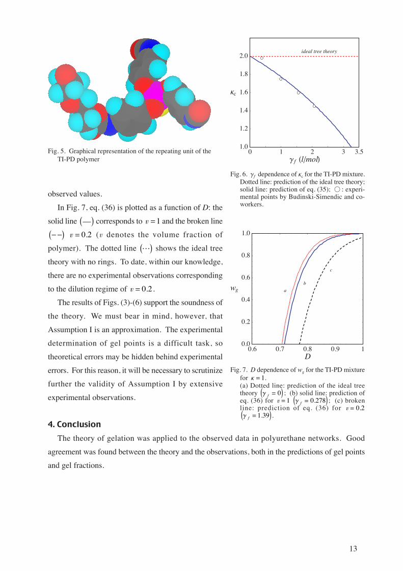
ideal tree theory

Fig. 5. Graphical representation of the repeating unit of theTI-PD polymer

Fig. 7. D dependence of wg for the TI-PD mixturefor Κ 1.(a) Dotted line: prediction of the ideal treetheory

Γ f 0 ; (b) solid line: prediction of

eq. (36) for v 1 Γ f 0 278. ; (c) broken

line: prediction of eq. (36) for v 0 2.

Γ f 1 39. .

0.6 0.7 0.8 0.9 1D

0.0

0.2

0.4

0.6

0.8

1.0

wg a

b

c

14

References

1. (a) Wile, L. L. Ph.D. dissertation, Columbia University, New York, 1945;

(b) Gordon, M. and Scantlebury, G. R. J. Chem. Soc., 1967, B, 1.

2. Flory, P. J. Principles of Polymer Chemistry, Cornell University Press, Ithaca, New York, 1953.

3. (a) Suematsu, K. Phys. Chem. Chem. Phys., 2002, 4, 4161;

(b) Macromol. Theory Simul., 2003, 12, 476.

4. (a) Isaacson, J. and Lubensky, T. C., J. Physique, 1980, 41, L-469;

(b) Zallen, R., Physics of Amorphous Solid, Wiley, New York, 1983;

(c) Westermann, S., Willner, L., Richter, D., and Fetters, L. J.,

Macromol. Chem. Phys., 2000, 201, 500;

(d) Graessley, W. W., Macromolecules, 2002, 35, 3184.

5. (a) Spouge, J. L., Proc. R. Soc. Lond., 1983, A 387, 351;

(b) J. Stat. Phys., 1986, 43, 363.

6. Essam, J. W., Rep. Prog. Phys., 1980, 43, 53.

7. de Dennes, P. G., Scaling Concepts in Polymer Physics, Cornell University Press, Ithaca and

London, 1979.

8. Ziff, R. M. and Stell, G., J. Chem. Phys., 1980, 73, 3492.

9. (a) Ilavsky, M. and Dusek, K., Macromolecules, 1986, 19, 2139; (b) Polymer, 1983, 24, 981.

10. (a) Adam, M., Delsanti, M., Munch, J. P., and Durand, D., J. Physique, 1987, 48, 1809;

(b) Adam, M., Delsanti, M., and Durand, D., Macromolecules, 1985, 18, 2285;

(c) Durand, D., Naveau, F., Busnel, J. P., Delsanti, M., and Adam, M., Macromolecules, 1989,

22, 2011.

11. Budinski-Simendic, J., Petrovic, Z. S., Ilavsky, M., and Dusek, K., Polymer, 1993, 34, 5157.