Theory of HPLC - chromacademy.com · Limit of Detection / Quantification (LOD / LOQ) 6 UV-Vis Detectors, The Flow ... chromatogram is treated as a starting point for the determination

Instrumentation of HPLC

Detectors

i Wherever you see this symbol, it is important to access the on-line course as there is interactive material that cannot be fully shown in this reference manual.

Aims and Objectives

Aims and Objectives

Aims

To describe the purpose and general operating principles of detectors for HPLC

To outline the general terms and concepts by which detector operation and performance are described

To describe specific operating principles of a range Detectors for HPLC, including: UV-Visible, Refractive Index and Fluorescence Detectors

Examine the advantages and functionality associated with Diode Array UV-Visible detection

Outline the basic nature of quantitative analysis by HPLC and investigate instrument calibration

To highlight the advantages and disadvantages of each detector type and to indicate the circumstances under which different detectors might be used

Objectives At the end of this Section you should be able to:

Describe the function of the detector in HPLC

Recognise and use the terms which are used to describe and measure detector performance

Demonstrate an understanding of the operating principles of the most popular detectors used for HPLC

Recognise when a Diode Array detector will bring benefits to the analysis

Understand the settings used to optimise Diode Array detection

Describe the general principles behind instrument calibration and the role of HPLC detectors in quantitative analysis

Recognise the advantages and disadvantages of each detector type and to chose the appropriate detector for a variety of analytical applications

© Crawford Scientific www.chromacademy.com

2

Content Detectors for HPLC –Introduction 3 General Terms and Concepts 4 Selectivity 4 Sensitivity 4 Limit of Detection / Quantification (LOD / LOQ) 6 UV-Vis Detectors, The Flow Cell 9 UV Detectors 9 UV-Vis Detectors, Quantitation 10 External Standard Quantitation 11 Calibration Curve 12 Statistical Information 13 UV-Vis Detectors, UV absorbance 14 Variable Wavelength UV-Vis Detectors 16 Detector sensitivity 17 UV Detectors –Diode Array Detectors 18 The orthogonal nature of diode array UV-Vis detector data 18 UV Detectors –DAD Spectra 20 DAD Detectors –Bandwidth 21 DAD Detectors –Slit Width 23 DAD Detectors –Response time 24 DAD Detectors –Reference Wavelength 25 Choosing Sample and Reference Settings 26 DAD –Peak Suppression 27 Fluorescence Detectors 28 Fluorescence Detectors –Principles 30 Fluorescence Detectors –Excitation & Emission 32 Refractive Index Detectors –Instrumentation 34 Refractive Index Detectors –Principles 37


3

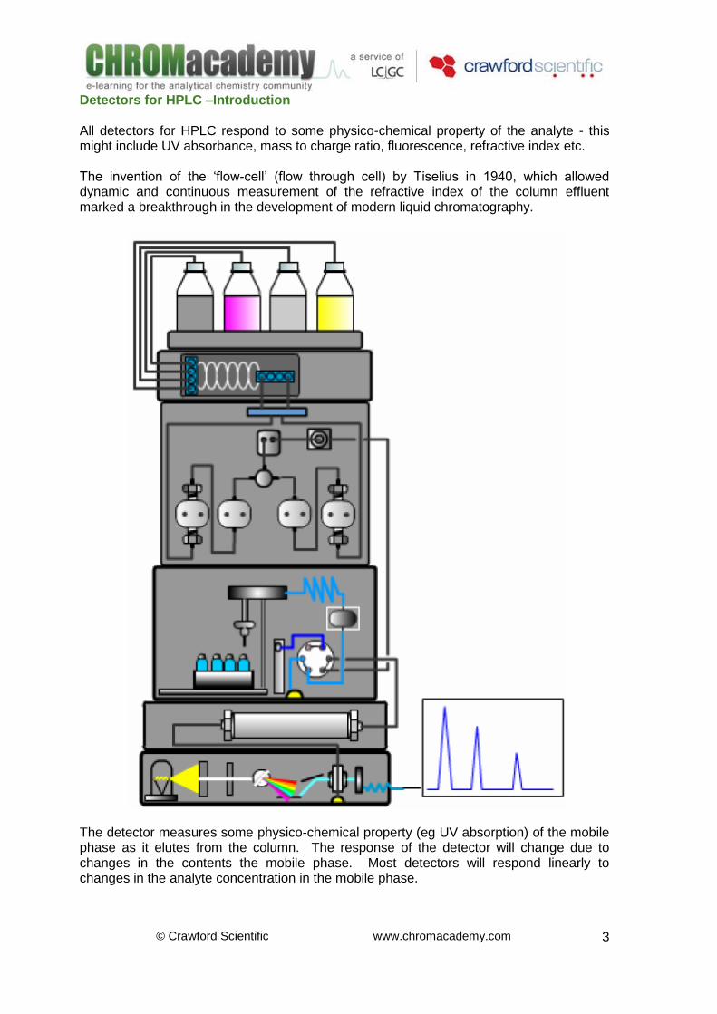
Detectors for HPLC –Introduction All detectors for HPLC respond to some physico-chemical property of the analyte - this might include UV absorbance, mass to charge ratio, fluorescence, refractive index etc. The invention of the ‘flow-cell’ (flow through cell) by Tiselius in 1940, which allowed dynamic and continuous measurement of the refractive index of the column effluent marked a breakthrough in the development of modern liquid chromatography.

The detector measures some physico-chemical property (eg UV absorption) of the mobile phase as it elutes from the column. The response of the detector will change due to changes in the contents the mobile phase. Most detectors will respond linearly to changes in the analyte concentration in the mobile phase.


4

The most common HPLC detectors are based on the absorbance of UV (or Visible) light by the analyte molecule. These detectors are popular because of their low cost, robustness, reasonably low detection limits, and ease of use. There are several common types of ‘UV’ detectors including; single wavelength, multiple wavelength or diode array configurations. The diode array detector also allows some limited qualitative functionality via the ability to dynamically collect UV spectra. Several other detector types are available which use other physico-chemical properties of the analyte molecule and these include:

Flouresence

Electrochemical

Electrical Conductivity These detectors tend to be employed when high sensitivity is required and/or the analyte molecule does not absorb UV radiation. Mass Spectrometric detectors have become increasingly important and these are now widely used in many areas of analytical chemistry as they can be used for the detection of low analyte concentrations, for qualitative analyses or in situations where separation of analyte components is difficult. Refractive index detection is useful when analyte molecules do not respond to any other detector type or if the analyte shows large differences in refractive index from the mobile phase used. The ideal detector should:

Either be equally sensitive to all eluted peaks or only record those of interest

Not be affected by changes in temperature or in mobile phase composition

Be able to monitor small amounts of compound (trace analysis)

Not contribute to band broadening (small cell volume)

React quickly to detect narrow peaks which pass through the cell

Be easy to manipulate and robust General Terms and Concepts Selectivity Non-selective detectors react to the bulk property of the solution passing into the detector. When a compound elutes from the column, this bulk property changes and the change is measured and recorded (i.e. refractive index). Selective detectors do not react to the bulk solution passing through but measure a response due to a specific property of the solute molecule (i.e. UV absorbance). Sensitivity The smallest detectable signal is usually estimated to be equivalent to three times the height of the average baseline noise – this would give a signal to noise ratio of 3:1 for the ‘Limit of Detection’ of the detector . If the amount of analyte injected is less than this, then the signal ceases to be distinguishable from noise. For quantitative analysis a signal to noise (S/N) ratio of 10:1 is recommended for the ‘Limit of Quantitation’.


5

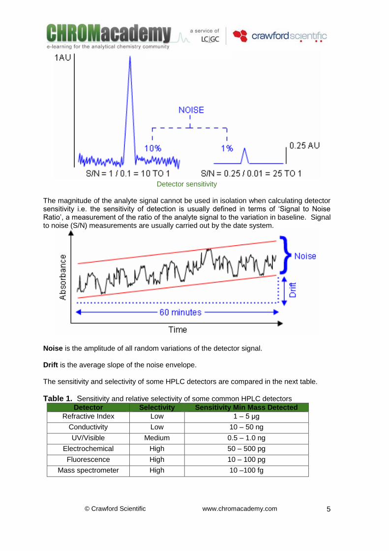
Detector sensitivity

The magnitude of the analyte signal cannot be used in isolation when calculating detector sensitivity i.e. the sensitivity of detection is usually defined in terms of ‘Signal to Noise Ratio’, a measurement of the ratio of the analyte signal to the variation in baseline. Signal to noise (S/N) measurements are usually carried out by the date system.

Noise is the amplitude of all random variations of the detector signal. Drift is the average slope of the noise envelope. The sensitivity and selectivity of some HPLC detectors are compared in the next table.

Table 1. Sensitivity and relative selectivity of some common HPLC detectors Detector Selectivity Sensitivity Min Mass Detected

Refractive Index Low 1 – 5 μg

Conductivity Low 10 – 50 ng

UV/Visible Medium 0.5 – 1.0 ng

Electrochemical High 50 – 500 pg

Fluorescence High 10 – 100 pg

Mass spectrometer High 10 –100 fg


6

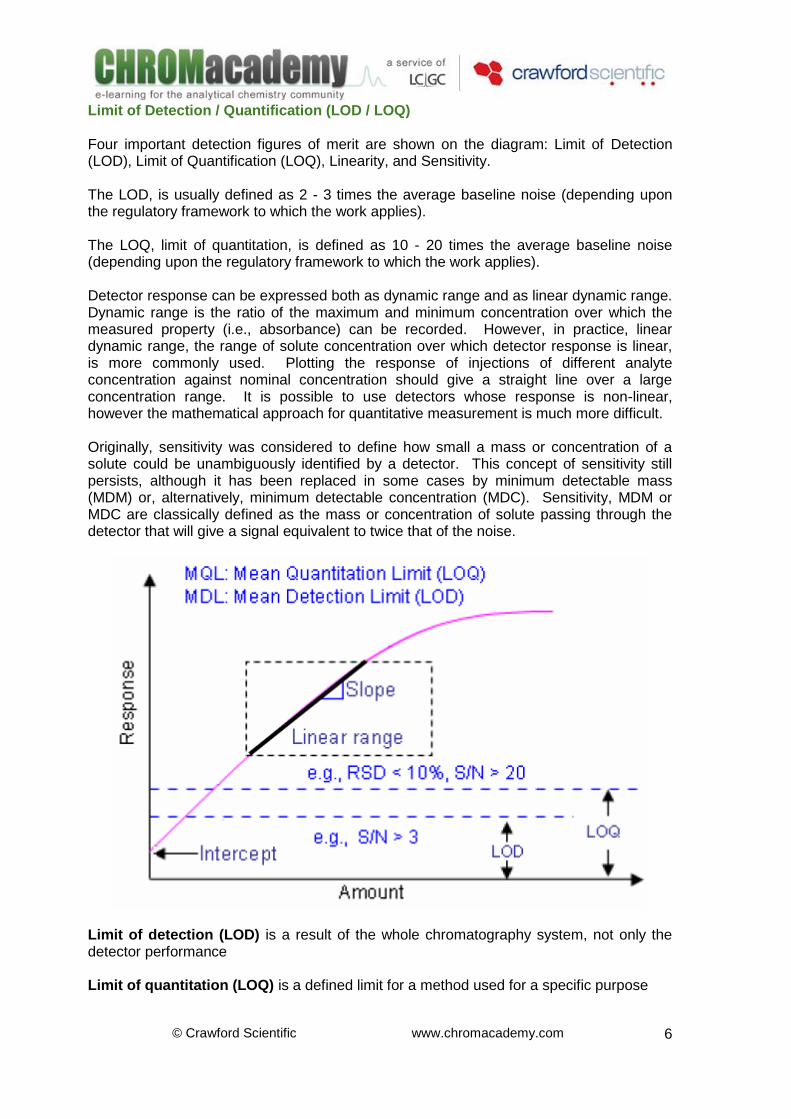
Limit of Detection / Quantification (LOD / LOQ) Four important detection figures of merit are shown on the diagram: Limit of Detection (LOD), Limit of Quantification (LOQ), Linearity, and Sensitivity. The LOD, is usually defined as 2 - 3 times the average baseline noise (depending upon the regulatory framework to which the work applies). The LOQ, limit of quantitation, is defined as 10 - 20 times the average baseline noise (depending upon the regulatory framework to which the work applies). Detector response can be expressed both as dynamic range and as linear dynamic range. Dynamic range is the ratio of the maximum and minimum concentration over which the measured property (i.e., absorbance) can be recorded. However, in practice, linear dynamic range, the range of solute concentration over which detector response is linear, is more commonly used. Plotting the response of injections of different analyte concentration against nominal concentration should give a straight line over a large concentration range. It is possible to use detectors whose response is non-linear, however the mathematical approach for quantitative measurement is much more difficult. Originally, sensitivity was considered to define how small a mass or concentration of a solute could be unambiguously identified by a detector. This concept of sensitivity still persists, although it has been replaced in some cases by minimum detectable mass (MDM) or, alternatively, minimum detectable concentration (MDC). Sensitivity, MDM or MDC are classically defined as the mass or concentration of solute passing through the detector that will give a signal equivalent to twice that of the noise.

Limit of detection (LOD) is a result of the whole chromatography system, not only the detector performance Limit of quantitation (LOQ) is a defined limit for a method used for a specific purpose


7

LOD (Limit of detection) –The minimum amount of analyte that can be reliably detected. The limit of detection, expressed as the concentration, cLl or the quantity, qL, is derived from the smallest measure, xL, that can be detected with reasonable certainty for a given analytical procedure. The value of xL is given by the equation

xL = xbi- + k × sbi Where: xbi- is the mean of the blank measurements sbi is the standard deviation of the blank measurements k is a numerical factor chosen according to the confidence level desired A sample that contains a complex matrix (e.g. environmental, biological sample) may show response from the matrix. RO determine the response a matrix sample without the compounds of interest should be analysed under same condition. The so called ‘blank’ chromatogram is treated as a starting point for the determination of LOD. The LOD is often defined as a ratio of S/N or peak area measurement precision. Examples of defining criteria are S/N ratio > 3 – peak height is compared to the noise height of the blank chromatogram to define the signal to noise ratio. Many modern data systems are capable of automatically providing a very accurate signal to noise ratio. LOQ (Limit of quantitation) –Lowest concentration of an analyte in a defined matrix where positive identification and quantitative measurement can be achieved using a specified method. The term ‘limit of quantitation’ is preferred to ‘limit of determination’ to differentiate it from LOD. LOQ has been defined as 3 times the LOD (Keith, 1991)or as 50% above the lowest calibration level used to validate the method (US-EPA, 1986). The LOQ is often defined as a ratio of S/N or peak area measurement precision and has much less stringent requirements than for limit of detection. Examples of definig criteria are S/N ratio > 20, or peak area precision better than 10%. The peak height is compared to the noise height of the blank chromatogram to define the signal to noise ratio. Many modern data systems are capable of automatically providing a very accurate signal to noise ratio. Intercept –The intercept of the calibration line indicates the degree of systematic error within the method and is the direct result of ‘background’ response. Many workers often include the results of a ‘blank analysis’ (i.e. where no analyte is added and x = 0) as a point in the calibration curve from which the regression line and regression co-efficient are obtained. Slope –The slope of the calibration line is often used to determine the sensitivity of the analytical method. Linear range –Concentration range over which the intensity of the signal obtained is directly proportional to the concentration of the species producing the signal. The linear range of a chromatographic detector represents the range of concentrations or mass flows of a substance in the mobile phase at the detector over which the sensitivity of the detector is constant within a specified variation, usually ±5 percent. The linear range of a detector may be presented as the plot of peak area (height) against concentration or mass flow-rate pf the test substance in the column effluent at the


8

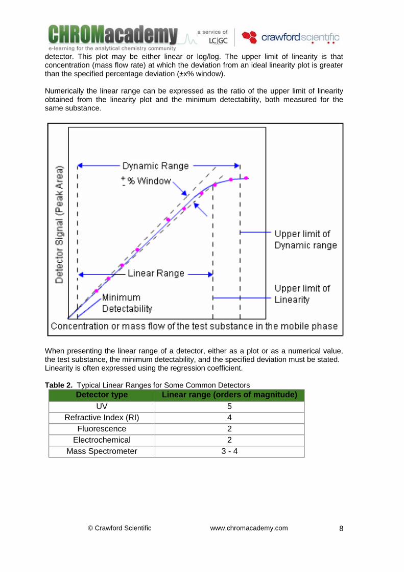
detector. This plot may be either linear or log/log. The upper limit of linearity is that concentration (mass flow rate) at which the deviation from an ideal linearity plot is greater than the specified percentage deviation (±x% window). Numerically the linear range can be expressed as the ratio of the upper limit of linearity obtained from the linearity plot and the minimum detectability, both measured for the same substance.

When presenting the linear range of a detector, either as a plot or as a numerical value, the test substance, the minimum detectability, and the specified deviation must be stated. Linearity is often expressed using the regression coefficient. Table 2. Typical Linear Ranges for Some Common Detectors

Detector type Linear range (orders of magnitude)

UV 5

Refractive Index (RI) 4

Fluorescence 2

Electrochemical 2

Mass Spectrometer 3 - 4


9

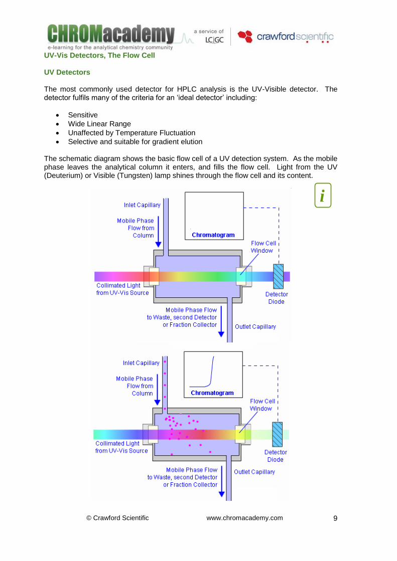
UV-Vis Detectors, The Flow Cell UV Detectors The most commonly used detector for HPLC analysis is the UV-Visible detector. The detector fulfils many of the criteria for an ‘ideal detector’ including:

Sensitive

Wide Linear Range

Unaffected by Temperature Fluctuation

Selective and suitable for gradient elution The schematic diagram shows the basic flow cell of a UV detection system. As the mobile phase leaves the analytical column it enters, and fills the flow cell. Light from the UV (Deuterium) or Visible (Tungsten) lamp shines through the flow cell and its content.

i


10

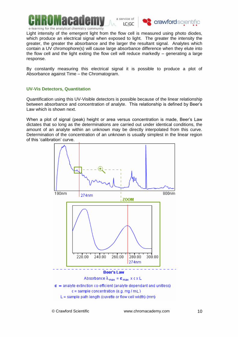
Light intensity of the emergent light from the flow cell is measured using photo diodes, which produce an electrical signal when exposed to light. The greater the intensity the greater, the greater the absorbance and the larger the resultant signal. Analytes which contain a UV chromophore(s) will cause large absorbance difference when they elute into the flow cell and the light exiting the flow cell will reduce markedly – generating a large response. By constantly measuring this electrical signal it is possible to produce a plot of Absorbance against Time – the Chromatogram. UV-Vis Detectors, Quantitation Quantification using this UV-Visible detectors is possible because of the linear relationship between absorbance and concentration of analyte. This relationship is defined by Beer’s Law which is shown next. When a plot of signal (peak) height or area versus concentration is made, Beer’s Law dictates that so long as the determinations are carried out under identical conditions, the amount of an analyte within an unknown may be directly interpolated from this curve. Determination of the concentration of an unknown is usually simplest in the linear region of this ‘calibration’ curve.


11

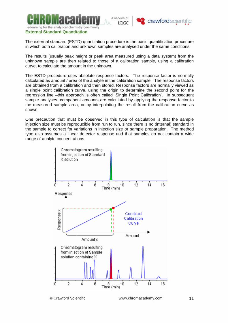
External Standard Quantitation The external standard (ESTD) quantitation procedure is the basic quantification procedure in which both calibration and unknown samples are analysed under the same conditions. The results (usually peak height or peak area measured using a data system) from the unknown sample are then related to those of a calibration sample, using a calibration curve, to calculate the amount in the unknown. The ESTD procedure uses absolute response factors. The response factor is normally calculated as amount / area of the analyte in the calibration sample. The response factors are obtained from a calibration and then stored. Response factors are normally viewed as a single point calibration curve, using the origin to determine the second point for the regression line –this approach is often called ‘Single Point Calibration’. In subsequent sample analyses, component amounts are calculated by applying the response factor to the measured sample area, or by interpolating the result from the calibration curve as shown. One precaution that must be observed in this type of calculation is that the sample injection size must be reproducible from run to run, since there is no (internal) standard in the sample to correct for variations in injection size or sample preparation. The method type also assumes a linear detector response and that samples do not contain a wide range of analyte concentrations.


12

Example:

analyteofamount

areapeakfactorresponse

factorresponse

areapeakanalyteofamount

An injection containing benzene at a concentration of 2000μg/mL is made and results in a peak area of 100000. The response factor for benzene:

502000

100000factorresponse

An injection of the sample with the unknown concentration of benzene has a peak area of 57000. The amount of benzene present in the sample:

gsampletheinbenzeneofAmount 114050

57000

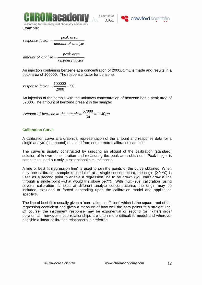
Calibration Curve A calibration curve is a graphical representation of the amount and response data for a single analyte (compound) obtained from one or more calibration samples. The curve is usually constructed by injecting an aliquot of the calibration (standard) solution of known concentration and measuring the peak area obtained. Peak height is sometimes used but only in exceptional circumstances. A line of best fit (regression line) is used to join the points of the curve obtained. When only one calibration sample is used (i.e. at a single concentration), the origin (X0:Y0) is used as a second point to enable a regression line to be drawn (you can’t draw a line through a single point –what would the slope be??). With multi-level calibration (using several calibration samples at different analyte concentrations), the origin may be included, excluded or forced depending upon the calibration model and application specifics. The line of best fit is usually given a ‘correlation coefficient’ which is the square root of the regression coefficient and gives a measure of how well the data points fit a straight line. Of course, the instrument response may be exponential or second (or higher) order polynomial –however these relationships are often more difficult to model and wherever possible a linear calibration relationship is preferred.


13

Multi(3) –level calibration curve

Statistical Information


14

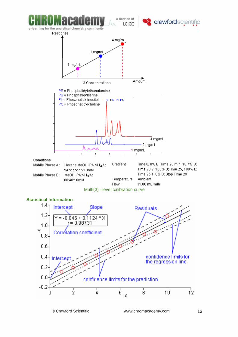
The intercept of the regression equation indicates a systematic error –a large positive or negative value may indicate an inherent error within the sample preparation of analysis. The slope of the line indicates the analytical ‘sensitivity’. The regression co-efficient is a statistical measure for ‘goodness of fit’ to a straight line, calculated using the residuals (error) of each data point, an r value of +1 indicates a straight line with positive slope. Some typical ‘r’ values are shown below –It is important to always plot data to check the fit.

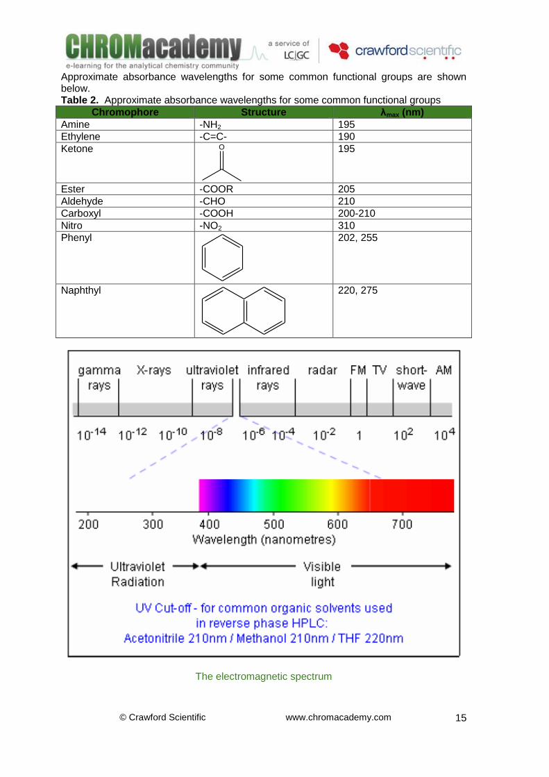
As can be seen from the examples –r values can be misleading! Workers sometimes use an r2 value which is statistically more rigorous. UV-Vis Detectors, UV absorbance In UV-Visible detection, the useful detection wavelength range is between 210 nm and 850 nm (with a tungsten lamp). Deuterium lamps are used for excitation of analyte molecules in the UV region (~180 – 380nm), Tungsten lamps are used for measurements in the visible region (380 – 800nm). Below about 210nm it is possible for the solvent used in the mobile phase to interfere with the analyte absorbance measurement. Electrons tightly bound in single carbon/carbon or carbon hydrogen bonds absorb electromagnetic energies corresponding to wavelengths less than 180 nm - below the useful operating range for a typical UV-Vis detector. Analyte molecules containing only C-C or C-H bonds do not show high sensitivity in UV-Vis detectors. Unshared electrons in the outer orbital’s of constituent atoms may exhibit larger absorbance’s in the useful range. This would include the unshared electrons of sulfur, bromine, and iodine. Electrons within unsaturated system such as double or triple bonds within organic molecules are relatively easily excited by UV radiation, and generally show absorbance within the useful UV-Visible region of the spectrum. Therefore, compounds with unsaturated and aromatic characteristics generally exhibit useful absorbance spectra.


15

Approximate absorbance wavelengths for some common functional groups are shown below. Table 2. Approximate absorbance wavelengths for some common functional groups

Chromophore Structure λmax (nm)

Amine -NH2 195

Ethylene -C=C- 190

Ketone O

195

Ester -COOR 205

Aldehyde -CHO 210

Carboxyl -COOH 200-210

Nitro -NO2 310

Phenyl

202, 255

Naphthyl

220, 275

The electromagnetic spectrum


16

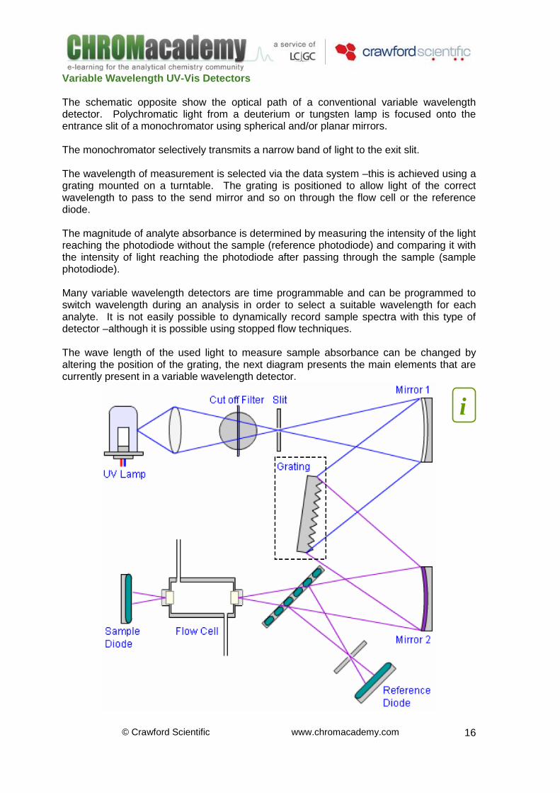
Variable Wavelength UV-Vis Detectors The schematic opposite show the optical path of a conventional variable wavelength detector. Polychromatic light from a deuterium or tungsten lamp is focused onto the entrance slit of a monochromator using spherical and/or planar mirrors. The monochromator selectively transmits a narrow band of light to the exit slit. The wavelength of measurement is selected via the data system –this is achieved using a grating mounted on a turntable. The grating is positioned to allow light of the correct wavelength to pass to the send mirror and so on through the flow cell or the reference diode. The magnitude of analyte absorbance is determined by measuring the intensity of the light reaching the photodiode without the sample (reference photodiode) and comparing it with the intensity of light reaching the photodiode after passing through the sample (sample photodiode). Many variable wavelength detectors are time programmable and can be programmed to switch wavelength during an analysis in order to select a suitable wavelength for each analyte. It is not easily possible to dynamically record sample spectra with this type of detector –although it is possible using stopped flow techniques. The wave length of the used light to measure sample absorbance can be changed by altering the position of the grating, the next diagram presents the main elements that are currently present in a variable wavelength detector.

i


17

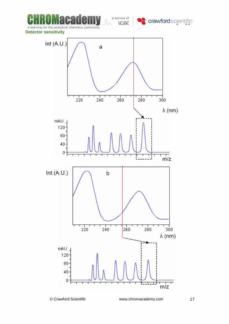
Detector sensitivity


18

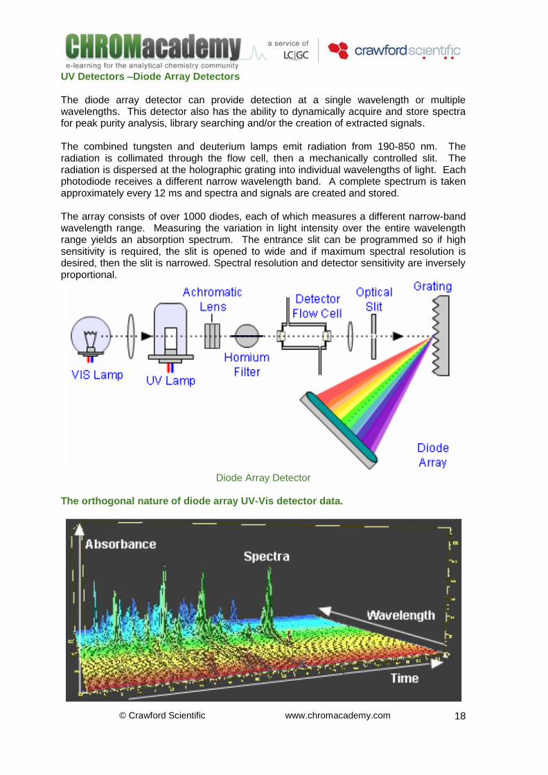
UV Detectors –Diode Array Detectors The diode array detector can provide detection at a single wavelength or multiple wavelengths. This detector also has the ability to dynamically acquire and store spectra for peak purity analysis, library searching and/or the creation of extracted signals. The combined tungsten and deuterium lamps emit radiation from 190-850 nm. The radiation is collimated through the flow cell, then a mechanically controlled slit. The radiation is dispersed at the holographic grating into individual wavelengths of light. Each photodiode receives a different narrow wavelength band. A complete spectrum is taken approximately every 12 ms and spectra and signals are created and stored. The array consists of over 1000 diodes, each of which measures a different narrow-band wavelength range. Measuring the variation in light intensity over the entire wavelength range yields an absorption spectrum. The entrance slit can be programmed so if high sensitivity is required, the slit is opened to wide and if maximum spectral resolution is desired, then the slit is narrowed. Spectral resolution and detector sensitivity are inversely proportional.

Diode Array Detector

The orthogonal nature of diode array UV-Vis detector data.


19

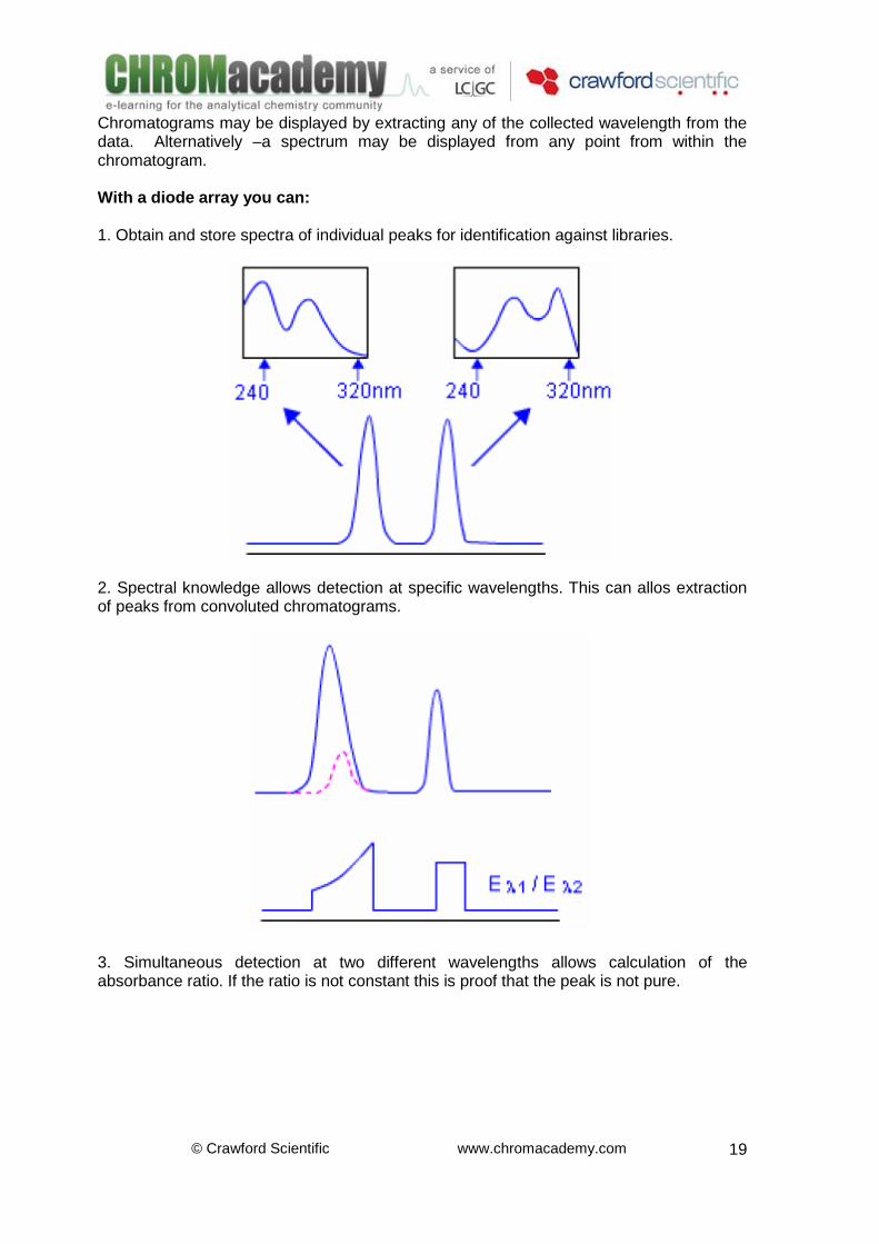
Chromatograms may be displayed by extracting any of the collected wavelength from the data. Alternatively –a spectrum may be displayed from any point from within the chromatogram. With a diode array you can: 1. Obtain and store spectra of individual peaks for identification against libraries.

2. Spectral knowledge allows detection at specific wavelengths. This can allos extraction of peaks from convoluted chromatograms.

3. Simultaneous detection at two different wavelengths allows calculation of the absorbance ratio. If the ratio is not constant this is proof that the peak is not pure.


20

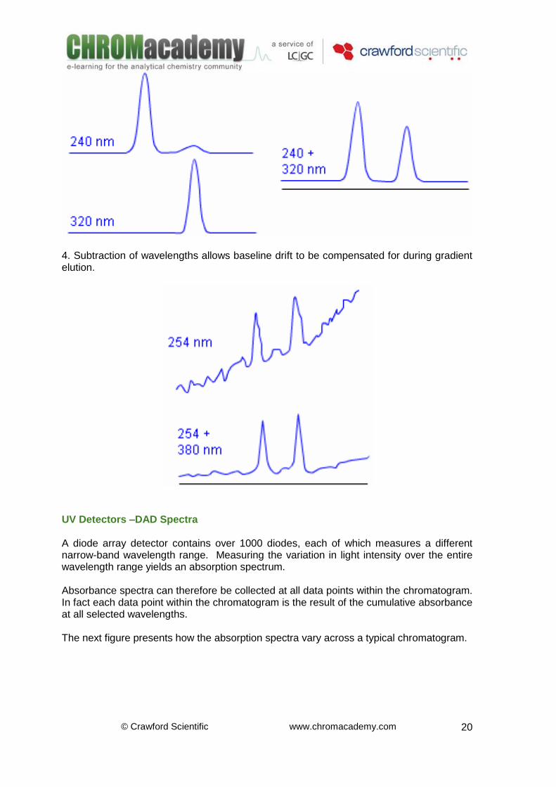
4. Subtraction of wavelengths allows baseline drift to be compensated for during gradient elution.

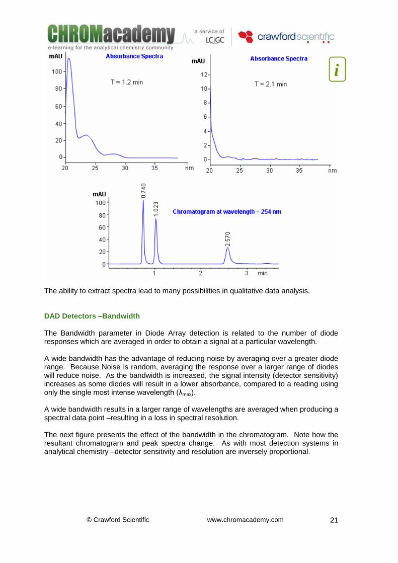
UV Detectors –DAD Spectra A diode array detector contains over 1000 diodes, each of which measures a different narrow-band wavelength range. Measuring the variation in light intensity over the entire wavelength range yields an absorption spectrum. Absorbance spectra can therefore be collected at all data points within the chromatogram. In fact each data point within the chromatogram is the result of the cumulative absorbance at all selected wavelengths. The next figure presents how the absorption spectra vary across a typical chromatogram.


21

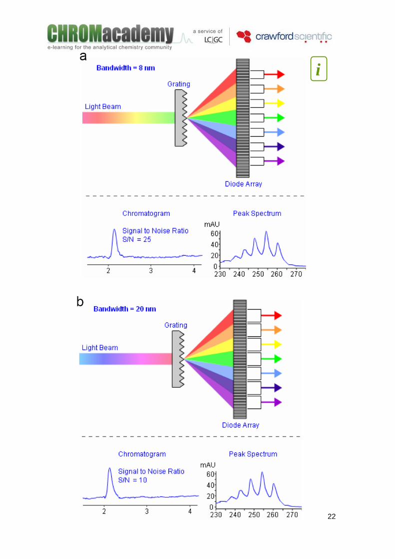
The ability to extract spectra lead to many possibilities in qualitative data analysis. DAD Detectors –Bandwidth The Bandwidth parameter in Diode Array detection is related to the number of diode responses which are averaged in order to obtain a signal at a particular wavelength. A wide bandwidth has the advantage of reducing noise by averaging over a greater diode range. Because Noise is random, averaging the response over a larger range of diodes will reduce noise. As the bandwidth is increased, the signal intensity (detector sensitivity) increases as some diodes will result in a lower absorbance, compared to a reading using only the single most intense wavelength (λmax). A wide bandwidth results in a larger range of wavelengths are averaged when producing a spectral data point –resulting in a loss in spectral resolution. The next figure presents the effect of the bandwidth in the chromatogram. Note how the resultant chromatogram and peak spectra change. As with most detection systems in analytical chemistry –detector sensitivity and resolution are inversely proportional.

i


22

i


23

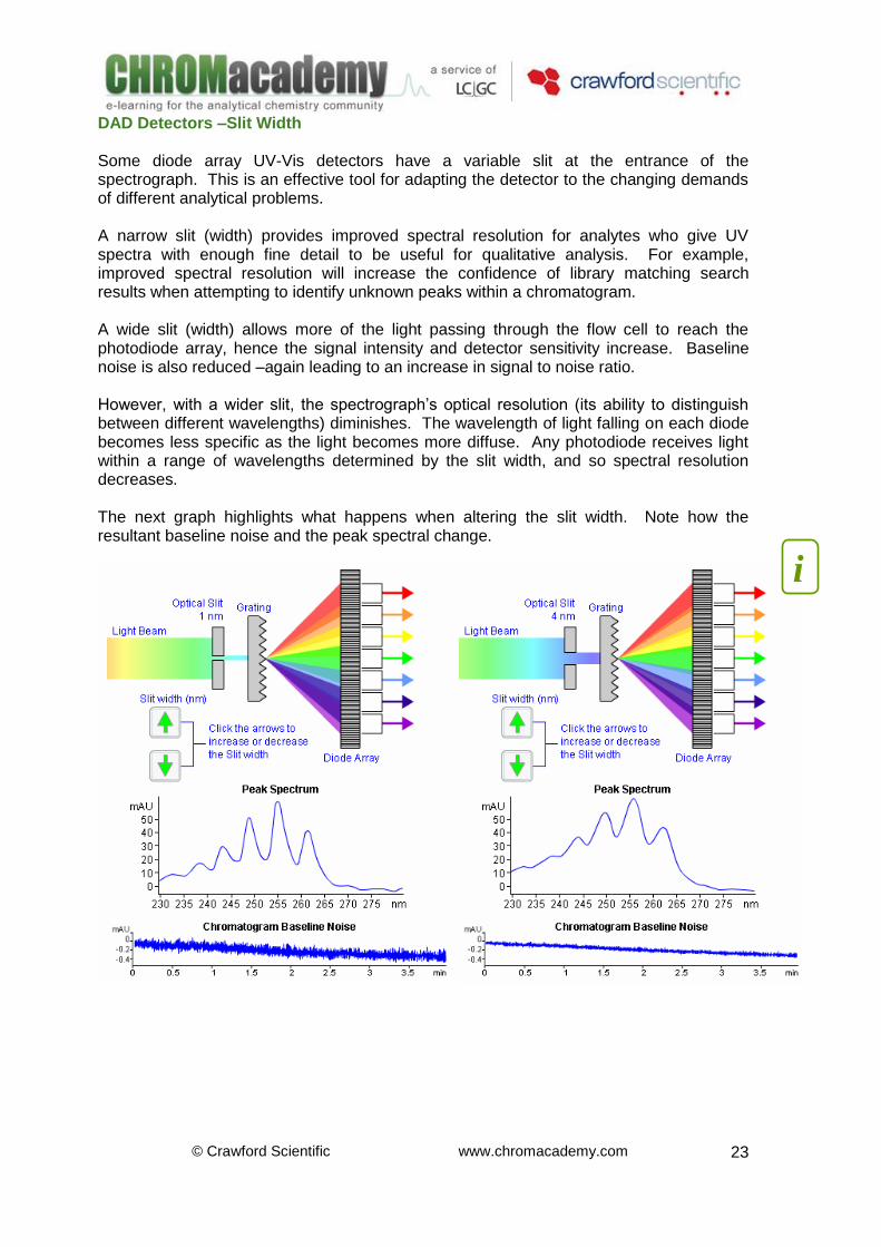
DAD Detectors –Slit Width Some diode array UV-Vis detectors have a variable slit at the entrance of the spectrograph. This is an effective tool for adapting the detector to the changing demands of different analytical problems. A narrow slit (width) provides improved spectral resolution for analytes who give UV spectra with enough fine detail to be useful for qualitative analysis. For example, improved spectral resolution will increase the confidence of library matching search results when attempting to identify unknown peaks within a chromatogram. A wide slit (width) allows more of the light passing through the flow cell to reach the photodiode array, hence the signal intensity and detector sensitivity increase. Baseline noise is also reduced –again leading to an increase in signal to noise ratio. However, with a wider slit, the spectrograph’s optical resolution (its ability to distinguish between different wavelengths) diminishes. The wavelength of light falling on each diode becomes less specific as the light becomes more diffuse. Any photodiode receives light within a range of wavelengths determined by the slit width, and so spectral resolution decreases. The next graph highlights what happens when altering the slit width. Note how the resultant baseline noise and the peak spectral change.

i


24

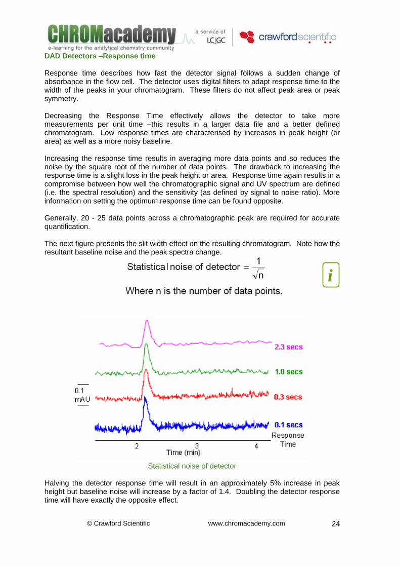
DAD Detectors –Response time Response time describes how fast the detector signal follows a sudden change of absorbance in the flow cell. The detector uses digital filters to adapt response time to the width of the peaks in your chromatogram. These filters do not affect peak area or peak symmetry. Decreasing the Response Time effectively allows the detector to take more measurements per unit time –this results in a larger data file and a better defined chromatogram. Low response times are characterised by increases in peak height (or area) as well as a more noisy baseline. Increasing the response time results in averaging more data points and so reduces the noise by the square root of the number of data points. The drawback to increasing the response time is a slight loss in the peak height or area. Response time again results in a compromise between how well the chromatographic signal and UV spectrum are defined (i.e. the spectral resolution) and the sensitivity (as defined by signal to noise ratio). More information on setting the optimum response time can be found opposite. Generally, 20 - 25 data points across a chromatographic peak are required for accurate quantification. The next figure presents the slit width effect on the resulting chromatogram. Note how the resultant baseline noise and the peak spectra change.

Statistical noise of detector

Halving the detector response time will result in an approximately 5% increase in peak height but baseline noise will increase by a factor of 1.4. Doubling the detector response time will have exactly the opposite effect.

i


25

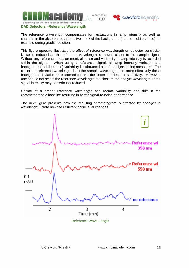
DAD Detectors –Reference Wavelength The reference wavelength compensates for fluctuations in lamp intensity as well as changes in the absorbance / refractive index of the background (i.e. the mobile phase) for example during gradient elution. This figure opposite illustrates the effect of reference wavelength on detector sensitivity. Noise is reduced as the reference wavelength is moved closer to the sample signal. Without any reference measurement, all noise and variability in lamp intensity is recorded within the signal. When using a reference signal, all lamp intensity variation and background (mobile phase) variability is subtracted out of the signal being measured. The closer the reference wavelength is to the sample wavelength, the more effectively these background deviations are catered for and the better the detector sensitivity. However, one should not select the reference wavelength too close to the analyte wavelength or the signal intensity may be seriously reduced. Choice of a proper reference wavelength can reduce variability and drift in the chromatographic baseline resulting in better signal-to-noise performance. The next figure presents how the resulting chromatogram is affected by changes in wavelength. Note how the resultant noise level changes.

Reference Wave Length.

i


26

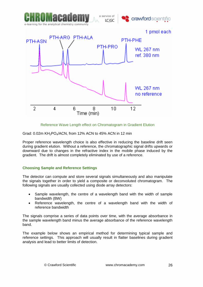
Reference Wave Length effect on Chromatogram in Gradient Elution Grad: 0.02m KH2PO4/ACN, from 12% ACN to 45% ACN in 12 min Proper reference wavelength choice is also effective in reducing the baseline drift seen during gradient elution. Without a reference, the chromatographic signal drifts upwards or downward due to changes in the refractive index in the mobile phase induced by the gradient. The drift is almost completely eliminated by use of a reference. Choosing Sample and Reference Settings The detector can compute and store several signals simultaneously and also manipulate the signals together in order to yield a composite or deconvoluted chromatogram. The following signals are usually collected using diode array detectors:

Sample wavelength, the centre of a wavelength band with the width of sample bandwidth (BW)

Reference wavelength, the centre of a wavelength band with the width of reference bandwidth

The signals comprise a series of data points over time, with the average absorbance in the sample wavelength band minus the average absorbance of the reference wavelength band. The example below shows an empirical method for determining typical sample and reference settings. This approach will usually result in flatter baselines during gradient analysis and lead to better limits of detection.


27

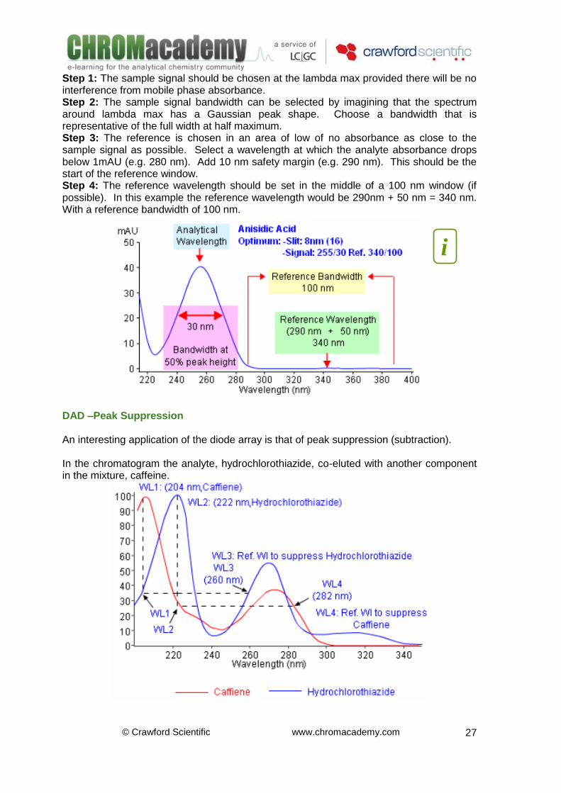
Step 1: The sample signal should be chosen at the lambda max provided there will be no interference from mobile phase absorbance. Step 2: The sample signal bandwidth can be selected by imagining that the spectrum around lambda max has a Gaussian peak shape. Choose a bandwidth that is representative of the full width at half maximum. Step 3: The reference is chosen in an area of low of no absorbance as close to the sample signal as possible. Select a wavelength at which the analyte absorbance drops below 1mAU (e.g. 280 nm). Add 10 nm safety margin (e.g. 290 nm). This should be the start of the reference window. Step 4: The reference wavelength should be set in the middle of a 100 nm window (if possible). In this example the reference wavelength would be 290nm + 50 nm = 340 nm. With a reference bandwidth of 100 nm.

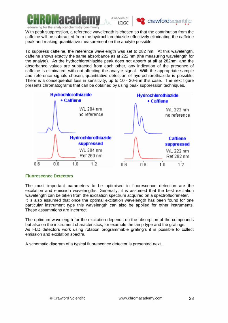
DAD –Peak Suppression An interesting application of the diode array is that of peak suppression (subtraction). In the chromatogram the analyte, hydrochlorothiazide, co-eluted with another component in the mixture, caffeine.

i


28

With peak suppression, a reference wavelength is chosen so that the contribution from the caffeine will be subtracted from the hydrochlorothiazide effectively eliminating the caffeine peak and making quantitative measurement on the analyte possible. To suppress caffeine, the reference wavelength was set to 282 nm. At this wavelength, caffeine shows exactly the same absorbance as at 222 nm (the measuring wavelength for the analyte). As the hydrochlorothiazide peak does not absorb at all at 282nm, and the absorbance values are subtracted from each other, any indication of the presence of caffeine is eliminated, with out affecting the analyte signal. With the appropriate sample and reference signals chosen, quantitative detection of hydrochlorothiazide is possible. There is a consequential loss in sensitivity, up to 10 - 30% in this case. The next figure presents chromatograms that can be obtained by using peak suppression techniques.

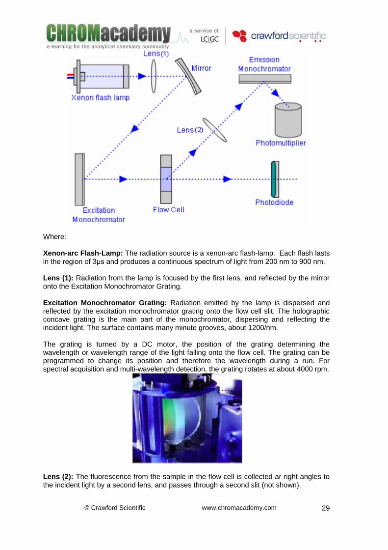
Fluorescence Detectors The most important parameters to be optimised in fluorescence detection are the excitation and emission wavelengths. Generally, it is assumed that the best excitation wavelength can be taken from the excitation spectrum acquired on a spectrofluorimeter. It is also assumed that once the optimal excitation wavelength has been found for one particular instrument type this wavelength can also be applied for other instruments. These assumptions are incorrect. The optimum wavelength for the excitation depends on the absorption of the compounds but also on the instrument characteristics, for example the lamp type and the gratings. As FLD detectors work using rotation programmable grating’s it is possible to collect emission and excitation spectra. A schematic diagram of a typical fluorescence detector is presented next.


29

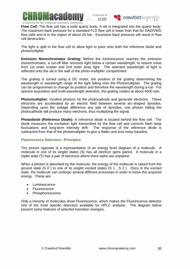
Where: Xenon-arc Flash-Lamp: The radiation source is a xenon-arc flash-lamp. Each flash lasts in the region of 3μs and produces a continuous spectrum of light from 200 nm to 900 nm. Lens (1): Radiation from the lamp is focused by the first lens, and reflected by the mirror onto the Excitation Monochromator Grating. Excitation Monochromator Grating: Radiation emitted by the lamp is dispersed and reflected by the excitation monochromator grating onto the flow cell slit. The holographic concave grating is the main part of the monochromator, dispersing and reflecting the incident light. The surface contains many minute grooves, about 1200/nm. The grating is turned by a DC motor, the position of the grating determining the wavelength or wavelength range of the light falling onto the flow cell. The grating can be programmed to change its position and therefore the wavelength during a run. For spectral acquisition and multi-wavelength detection, the grating rotates at about 4000 rpm.

Lens (2): The fluorescence from the sample in the flow cell is collected ar right angles to the incident light by a second lens, and passes through a second slit (not shown).


30

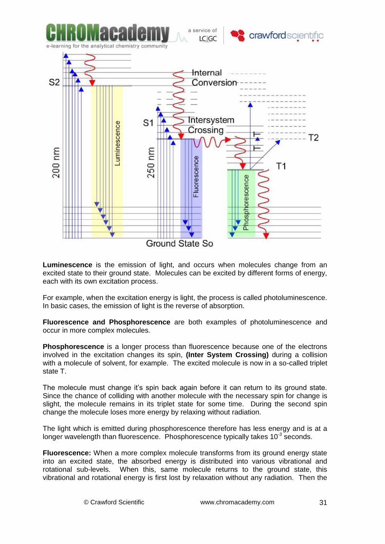
Flow Cell: The flow cell has a solid quartz body. A slit is integrated into the quartz body. The maximum back pressure for a standard FLD flow cell is lower than that for DAD/VWD flow cells and is in the region of about 20 bar. Excessive back pressure will result in flow cell destruction. The light is split in the flow cell to allow light to pass onto both the reference diode and photomultiplier. Emission Monochromator Grating: Before the luminescence reaches the emission monochromator, a cut-off filter removes light below a certain wavelength, to reduce noise from 1st order scatter and 2nd order stray light. The selected wavelength of light is reflected onto the slit in the wall of the photo-multiplier compartment. The grating is turned using a DC motor, the position of the grating determining the wavelength or wavelength range of the light falling onto the Photomultiplier. The grating can be programmed to change its position and therefore the wavelength during a run. For spectra acquisition and multi-wavelength detection, the grating rotates at about 4000 rpm. Photomultiplier: Incident photons hit the photocathode and generate electrons. These electrons are accelerated by an electric field between several arc-shaped dynodes. Depending upon the voltage difference any pair of dynodes, one photon hitting the photocathode will produce many electrons, thus multiplying the signal. Photodiode (Reference Diode): A reference diode is located behind the flow cell. The diode measures the excitation light transmitted by the flow cell and corrects flash lamp fluctuations and long-term intensity drift. The response of the reference diode is subtracted from that of the photomultiplier to give a flatter and less noisy baseline. Fluorescence Detectors –Principles The picture opposite is a representation of an energy level diagram of a molecule. A molecule in one of its singlet states (S) has all electron spins paired. A molecule in a triplet state (T) has a pair of electrons where there spins are unpaired. When a photon is absorbed by the molecule, the energy of the molecule is raised from the ground state (S 0 ) to one of its singlet excited states (S 1 , S 2 ). Once in the excited state, the molecule can undergo several different processes in order to loose the acquired energy. These are:

Luminescence

Fluorescence

Phosphorescence Only a minority of molecules show Fluorescence, which makes the Fluorescence detector one of the most specific detectors available for HPLC analysis. The diagram below present some features of selected transition energies.


31

Luminescence is the emission of light, and occurs when molecules change from an excited state to their ground state. Molecules can be excited by different forms of energy, each with its own excitation process. For example, when the excitation energy is light, the process is called photoluminescence. In basic cases, the emission of light is the reverse of absorption. Fluorescence and Phosphorescence are both examples of photoluminescence and occur in more complex molecules. Phosphorescence is a longer process than fluorescence because one of the electrons involved in the excitation changes its spin, (Inter System Crossing) during a collision with a molecule of solvent, for example. The excited molecule is now in a so-called triplet state T. The molecule must change it’s spin back again before it can return to its ground state. Since the chance of colliding with another molecule with the necessary spin for change is slight, the molecule remains in its triplet state for some time. During the second spin change the molecule loses more energy by relaxing without radiation. The light which is emitted during phosphorescence therefore has less energy and is at a longer wavelength than fluorescence. Phosphorescence typically takes 10-3 seconds. Fluorescence: When a more complex molecule transforms from its ground energy state into an excited state, the absorbed energy is distributed into various vibrational and rotational sub-levels. When this, same molecule returns to the ground state, this vibrational and rotational energy is first lost by relaxation without any radiation. Then the


32

molecule transforms from this energy level to one of the vibrational and rotational sub-levels of its ground state, emitting light. Internal conversion, a transition from S2 to S1 is highly favored because there are typically excited levels in the next lowest singlet state that have the same energy as the higher energy singlet state. If a molecule emits light 10 –9 to 10-5 seconds after it was illuminated then the process is fluorescence.

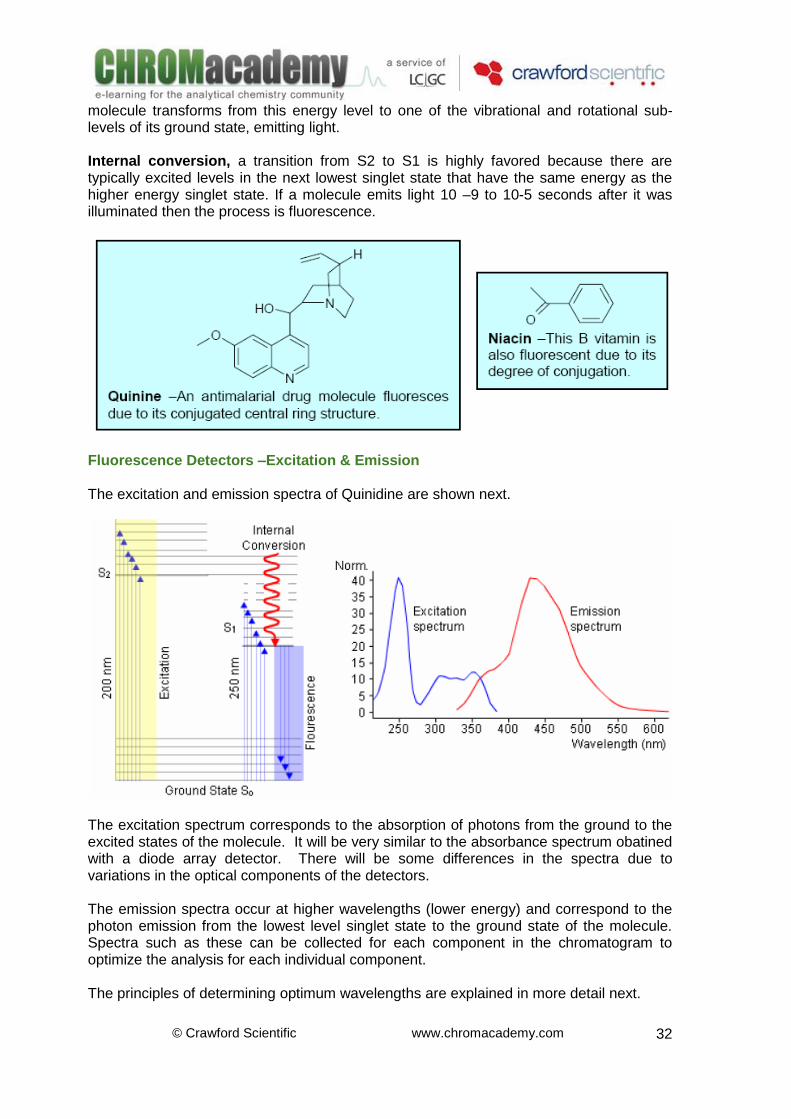
Fluorescence Detectors –Excitation & Emission The excitation and emission spectra of Quinidine are shown next.

The excitation spectrum corresponds to the absorption of photons from the ground to the excited states of the molecule. It will be very similar to the absorbance spectrum obatined with a diode array detector. There will be some differences in the spectra due to variations in the optical components of the detectors. The emission spectra occur at higher wavelengths (lower energy) and correspond to the photon emission from the lowest level singlet state to the ground state of the molecule. Spectra such as these can be collected for each component in the chromatogram to optimize the analysis for each individual component. The principles of determining optimum wavelengths are explained in more detail next.


33

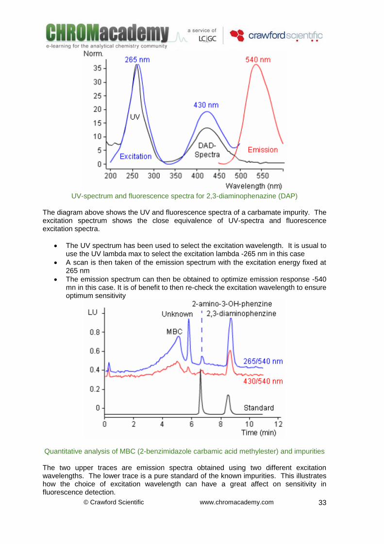
UV-spectrum and fluorescence spectra for 2,3-diaminophenazine (DAP)

The diagram above shows the UV and fluorescence spectra of a carbamate impurity. The excitation spectrum shows the close equivalence of UV-spectra and fluorescence excitation spectra.

The UV spectrum has been used to select the excitation wavelength. It is usual to use the UV lambda max to select the excitation lambda -265 nm in this case

A scan is then taken of the emission spectrum with the excitation energy fixed at 265 nm

The emission spectrum can then be obtained to optimize emission response -540 mn in this case. It is of benefit to then re-check the excitation wavelength to ensure optimum sensitivity

Quantitative analysis of MBC (2-benzimidazole carbamic acid methylester) and impurities The two upper traces are emission spectra obtained using two different excitation wavelengths. The lower trace is a pure standard of the known impurities. This illustrates how the choice of excitation wavelength can have a great affect on sensitivity in fluorescence detection.


34

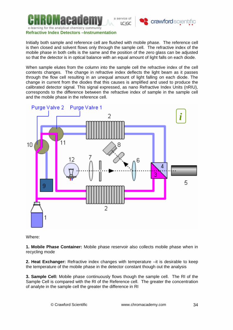
Refractive Index Detectors –Instrumentation Initially both sample and reference cell are flushed with mobile phase. The reference cell is then closed and solvent flows only through the sample cell. The refractive index of the mobile phase in both cells is the same and the position of the zero glass can be adjusted so that the detector is in optical balance with an equal amount of light falls on each diode. When sample elutes from the column into the sample cell the refractive index of the cell contents changes. The change in refractive index deflects the light beam as it passes through the flow cell resulting in an unequal amount of light falling on each diode. The change in current from the diodes that this causes is amplified and used to produce the calibrated detector signal. This signal expressed, as nano Refractive Index Units (nRIU), corresponds to the difference between the refractive index of sample in the sample cell and the mobile phase in the reference cell.

Where: 1. Mobile Phase Container: Mobile phase reservoir also collects mobile phase when in recycling mode 2. Heat Exchanger: Refractive index changes with temperature –it is desirable to keep the temperature of the mobile phase in the detector constant though out the analysis 3. Sample Cell: Mobile phase continuously flows though the sample cell. The RI of the Sample Cell is compared with the RI of the Reference cell. The greater the concentration of analyte in the sample cell the greater the difference in RI

i


35

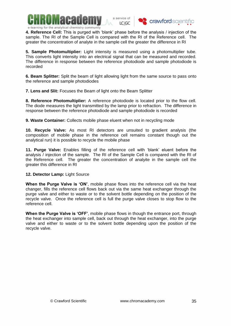
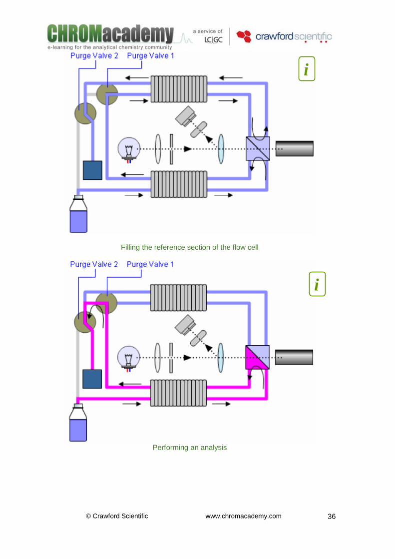
4. Reference Cell: This is purged with ‘blank’ phase before the analysis / injection of the sample. The RI of the Sample Cell is compared with the RI of the Reference cell. The greater the concentration of analyte in the sample cell the greater the difference in RI 5. Sample Photomultiplier: Light intensity is measured using a photomultiplier tube. This converts light intensity into an electrical signal that can be measured and recorded. The difference in response between the reference photodiode and sample photodiode is recorded 6. Beam Splitter: Split the beam of light allowing light from the same source to pass onto the reference and sample photodiodes 7. Lens and Slit: Focuses the Beam of light onto the Beam Splitter 8. Reference Photomultiplier: A reference photodiode is located prior to the flow cell. The diode measures the light transmitted by the lamp prior to refraction. The difference in response between the reference photodiode and sample photodiode is recorded 9. Waste Container: Collects mobile phase eluent when not in recycling mode 10. Recycle Valve: As most RI detectors are unsuited to gradient analysis (the composition of mobile phase in the reference cell remains constant though out the analytical run) it is possible to recycle the mobile phase 11. Purge Valve: Enables filling of the reference cell with ‘blank’ eluent before the analysis / injection of the sample. The RI of the Sample Cell is compared with the RI of the Reference cell. The greater the concentration of analyite in the sample cell the greater this difference in RI 12. Detector Lamp: Light Source When the Purge Valve is ‘ON’, mobile phase flows into the reference cell via the heat changer, fills the reference cell flows back out via the same heat exchanger through the purge valve and either to waste or to the solvent bottle depending on the position of the recycle valve. Once the reference cell is full the purge valve closes to stop flow to the reference cell. When the Purge Valve is ‘OFF’, mobile phase flows in though the entrance port, through the heat exchanger into sample cell, back out through the heat exchanger, into the purge valve and either to waste or to the solvent bottle depending upon the position of the recycle valve.


36

Filling the reference section of the flow cell

Performing an analysis

i

i


37

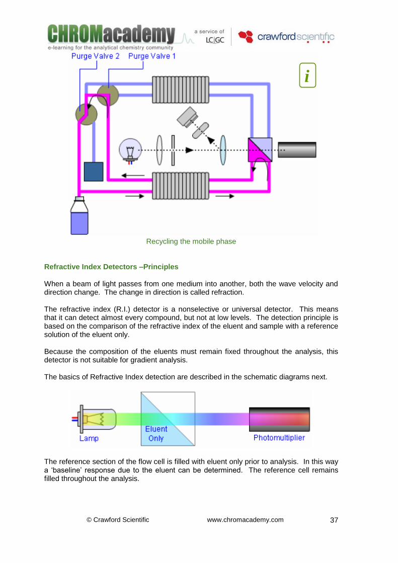
Recycling the mobile phase

Refractive Index Detectors –Principles When a beam of light passes from one medium into another, both the wave velocity and direction change. The change in direction is called refraction. The refractive index (R.I.) detector is a nonselective or universal detector. This means that it can detect almost every compound, but not at low levels. The detection principle is based on the comparison of the refractive index of the eluent and sample with a reference solution of the eluent only. Because the composition of the eluents must remain fixed throughout the analysis, this detector is not suitable for gradient analysis. The basics of Refractive Index detection are described in the schematic diagrams next.

The reference section of the flow cell is filled with eluent only prior to analysis. In this way a ‘baseline’ response due to the eluent can be determined. The reference cell remains filled throughout the analysis.

i


38

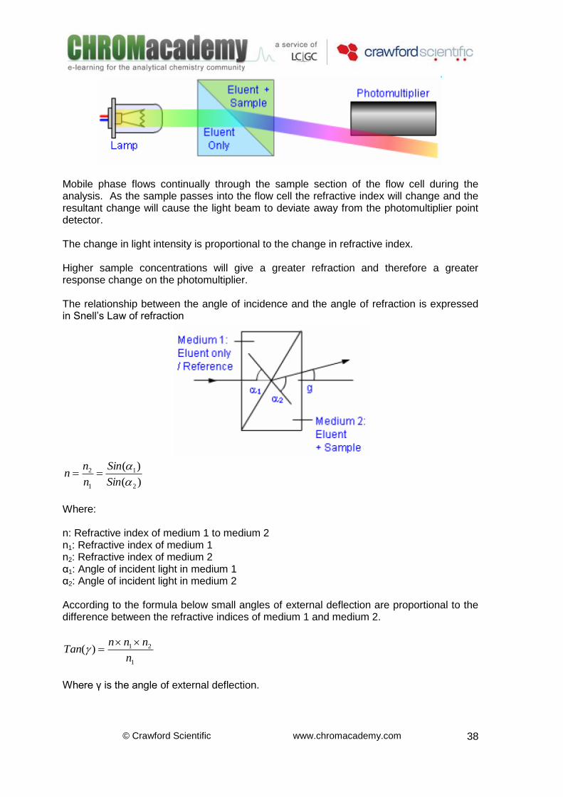
Mobile phase flows continually through the sample section of the flow cell during the analysis. As the sample passes into the flow cell the refractive index will change and the resultant change will cause the light beam to deviate away from the photomultiplier point detector. The change in light intensity is proportional to the change in refractive index. Higher sample concentrations will give a greater refraction and therefore a greater response change on the photomultiplier. The relationship between the angle of incidence and the angle of refraction is expressed in Snell’s Law of refraction

)(

)(

2

1

1

2

Sin

Sin

n

nn

Where: n: Refractive index of medium 1 to medium 2 n1: Refractive index of medium 1 n2: Refractive index of medium 2 α1: Angle of incident light in medium 1 α2: Angle of incident light in medium 2 According to the formula below small angles of external deflection are proportional to the difference between the refractive indices of medium 1 and medium 2.

1

21)(n

nnnTan

Where γ is the angle of external deflection.

Documents

Theory of HPLC - chromacademy.com · Limit of Detection / Quantification (LOD / LOQ) 6 UV-Vis Detectors, The Flow ... chromatogram is treated as a starting point for the determination