Embed Size (px)
Citation preview
1
Theory of Storage, Inventory and Volatility in the LME Base Metals
Hélyette Geman William O. Smith1
Director, Commodity Finance Centre
Birkbeck, University of London & ESCP Europe
Doctoral Programme
Birkbeck, University of London
Abstract
The theory of storage, as related to commodities, makes two predictions
involving the quantity of the commodity held in inventory. When inventory is low
(i.e. , a situation of scarcity), spot prices will exceed futures prices, and spot price
volatility will exceed futures price volatility. Conversely, during periods of no scarcity,
both spot prices and spot price volatility will remain relatively subdued. We test
these relationships for the six base metals traded on the London Metal Exchange
(aluminium, copper, lead, nickel, tin and zinc), and find strong validation for the
theory. Moreover, and in contrast to widespread claims that Chinese inventory
data are opaque, we find that including Chinese inventories strengthens the
relationship further. We also introduce the concepts of excess volatility, inventory-
implied spot price and inventory-implied spot volatility and illustrate some
applications.
JEL Categories: B 26, C22, G13, G31, N50, Q31
Keywords:
Working curve, storage, base metals, inventory, volatility, convenience yield, forward
curve
Forthcoming in Resources Policy, 2012
2
1. Introduction
The aim of this paper is to examine the six base metals traded on the LME
(aluminium, copper, lead, nickel, tin and zinc), and examine the relationship
between price, volatility and the quantity held in inventory, for both the spot and
futures markets. A relationship, believed to exist for many storable commodities, is
predicted by the Theory of Storage. In Section 1.1, we review briefly the base metals
and futures trading. In Section 1.2, we review the theory of storage and its literature
across a number of commodities. In Section 2, we review our data and develop a
gauge for inventory which permits comparison between commodities and over long
time periods. In Section 3, we examine the relationship between price and inventory,
and in Section 4 the relationship between volatility and inventory. In Section 5, we
consider some applications, and Section 6 concludes.
1.1 Base Metals and Futures Trading
Firstly, we review the base metals, futures markets (particularly the London Metal
Exchange) and the existing literature on the theory of storage.
1.1.1 The Base Metals
Unlike the precious metals such as gold and silver, which are often purchased
for investment rather than commercial use, the base metals are all notable for their
industrial uses, principally in automobiles (aluminium, nickel) , packaging (aluminum,
tin), building and infrastructure construction (aluminium, copper, nickel, zinc),
electronic and electrical components (copper, lead, tin) and many other
applications.
Prices of the base metals vary according to their rarity and extraction costs,
ranging from around $25,000 per tonne (nickel, tin), through $10,000 per tonne
(copper) down to around $2,500 per tonne (aluminum, lead, zinc), observed in mid-
2011. They are typically traded on the LME in the form of bars, rods or ingots, with
the exact contract specifications being tailored to the typical requirements of
industrial users, and at high purities in excess of 99.8%.
Unlike many commodities, the base metals show negligible seasonal variation
in their supply and only minor seasonal variation in demand (related to slight
variations in construction activity across the northern hemisphere year), simplifying
3
their analysis. They are easily storable at relatively low cost (typically < 5% of their
value p.a.), and unlike agricultural commodities, suffer negligible degradation over
time, again simplifying their analysis.
1.1.2 Futures Markets
Commodity markets typically have greatest liquidity in futures markets rather
spot markets, which allows participants to ‘lock in’ a price in advance, for example
a farmer may wish to fix a price for his harvest long before harvest time, or a
construction company may wish to fix the price of copper they will use some months
hence. On any given trading date ‘ t ’, a number of futures contracts are traded,
one for each maturity date 1T to NT . Typically maturities range from 1 month to
several years into the future. The purchase of a futures contract obliges the owner
to pay on the maturity date , {1,..., }iT i N∈ ,the market price ( , )iF t T to the seller, and
in turn (s)he will receive one contract’s worth of commodities2. Typically futures are
traded on an exchange, and margin payments will be payable between the trade
date t and the maturity date iT to minimize the counterparty risk born by each side.
In addition, for some commodities, spot markets exist with immediate delivery
required. Where this is not the case, it is typical to consider the price of the futures
contract which is soonest to expire (the so-called ‘front month’ contract) as a proxy
for a spot price.
1.1.3 The London Metal Exchange
London has been the world hub of metal trading for centuries, in an area
near to the former Royal Exchange. Ad-hoc metal trading was replaced with a
formal exchange with the founding of the London Metal Exchange in 1877. The LME
has remained the centre of world metal trading ever since. Despite competition
from COMEX in the US, and the Shanghai Futures Exchange (SHFE) in China, it
remains for now the most liquid venue for trading of base metals. In particular, we
examine in this study its contracts for Aluminum, Copper, Lead, Nickel, Tin and Zinc.
2 Typically there may be some small lag comprising several business days between maturity of the contract and the delivery date, but this is irrelevant in the present context.
4
The LME’s trading structure is somewhat unique, resulting from its long history.
Several times a day, so called ‘ring’ trading sessions occur, in an open-outcry format,
with traders located physically in a seated circle or ring, with only a single metal
traded per brief and intense 5 minute session. Electronic trading is also available
during an extended business day, and telephone trading is available 24 hours per
day, with all trades reported and settled through the LME (LME 2011).
Unlike most commodity exchanges where futures contracts are typically
deliverable in fixed months, with only occasional ‘expiry’ of contracts, the LME
trades constant maturity contracts. On each trading day, contracts for delivery in 2
days (‘spot’), 3 months, 15 months and 27 months are traded. The 3-month contract
is the most heavily traded, and was originally introduced because it took that long
for tin from South-East Asia, or copper from Chile, to arrive by ship to London
(Bloomberg 2011).
The LME maintains a worldwide network of over 600 warehouses. Although
counterparties of a futures or spot trade are free to arrange bilaterally the delivery of
metal from seller to buyer, they can also deliver to or take delivery from an LME
warehouse. The warehouses are carefully chosen worldwide to be at sources of
demand rather than supply, ensuring that the buyer has immediate access to the
metal he has purchased (LME 2011b). However, to date, China does not allow
warehouses in its territory to become LME-registered, and metal for Chinese delivery
is typically shipped from Singapore or South Korea. Inventory figures across all
warehouses are published daily.
1.2 Commodity Inventories and the Theory of Storage
Commodities can be categorized as storable or non-storable. Non-storable
commodities include those where storage methods exist but are prohibitively
expensive (in particular, the case of electricity) and where the commodity is the
provision of a service (as in the shipping industry). The vast majority of commodities
are storable. They are stored for several reasons:
• As a buffer against uneven or seasonal supply, as in the case of agricultural
commodities, which have been stored in silos as early as 10,000 years ago
5
• As a buffer against uneven demand, as in the case of most energy
commodities, which are typically used more in winter for heating, and
midsummer for cooling
• As a buffer against any other supply or logistical disruption, which would
otherwise necessitate the expensive pause of an industrial process
• In recent years, for investment purposes within physically-backed ETFs
• For arbitrage reasons, if any, as described later.
The theory of storage applies to any commodity that can be physically stored
and makes two main predictions, both related to the quantity of the commodity
held in inventory (also known as stocks, a term we avoid due to its confusion with
equity markets).
1.2.1 Prediction 1, concerning the relationship between spot and futures prices.
When there is a situation of scarcity (low inventory), spot prices will rise as
purchasers bid whatever is necessary to secure supply. The effect will be less
pronounced in longer term futures, since market participants know that higher price
will, in the long term, stimulate increased supply and allow for a rebuilding of
inventory. The effect, with spot price > futures price, can be extreme, and is known
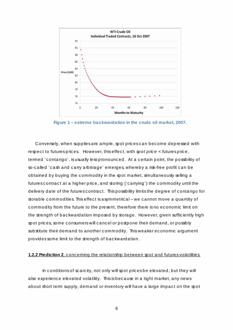
as ‘backwardation’. An example of backwardation in the crude oil futures market
is shown in Figure 1, taken from the time of high oil demand and rapid price rises in
2007. Oil contracts that mature (expire) in 40 or more months are priced around $76,
whereas those expiring within 1 month (so called ‘nearby’) futures are priced as high
as $89.
6
Figure 1 – extreme backwardation in the crude oil market, 2007.
Conversely, when supplies are ample, spot prices can become depressed with
respect to futures prices. However, this effect, with spot price < futures price,
termed ‘contango’, is usually less pronounced. At a certain point, the possibility of
so-called ‘cash and carry arbitrage’ emerges, whereby a risk-free profit can be
obtained by buying the commodity in the spot market, simultaneously selling a
futures contract at a higher price, and storing (‘carrying’) the commodity until the
delivery date of the futures contract. This possibility limits the degree of contango for
storable commodities. This effect is asymmetrical – we cannot move a quantity of
commodity from the future to the present, therefore there is no economic limit on
the strength of backwardation imposed by storage. However, given sufficiently high
spot prices, some consumers will cancel or postpone their demand, or possibly
substitute their demand to another commodity. This weaker economic argument
provides some limit to the strength of backwardation.
1.2.2 Prediction 2, concerning the relationship between spot and futures volatilities.
In conditions of scarcity, not only will spot prices be elevated, but they will
also experience elevated volatility. This is because in a tight market, any news
about short term supply, demand or inventory will have a large impact on the spot
7
market. However, there is little corresponding rise in the volatility of long term futures
contracts, whose prices mainly respond to longer-term news.
In conditions of abundance, this effect will disappear, and there will be no
pronounced difference between the volatility of spot and futures prices.
We note that in general, the so called ‘Samuelson effect’ (Samuelson 1965)
states that commodity futures becomes more volatile as they approach maturity,
although unlike the theory of storage, it does not mention that such conditions
mainly apply during scarcity. We might expect that spot price volatility will almost
always exceed futures price volatility, since long term prices mainly respond to long-
term news, whereas short-term prices should respond to both short and long term
news, as well as all kinds of “noise” induced by short term trading.
1.2.3 Development of the Theory of Storage –Inventory and Prices
We describe below the key architects of the theory of storage. In particular,
early and instrumental work seems to be regularly overlooked in the literature.
Empirical observation of futures markets had long noted that near-month
futures prices were often higher than long-term futures. Keynes (1930) first sought to
explain the empirical data by noting that long term futures were usually sold by
farmers wishing to fix a price for their harvest and therefore reduce their risk. The
futures were bought by speculators, willing to take on the risk in order to realise a
profit. Speculators would not enter the market, bearing risk, he argued, unless
futures prices tended to rise as harvest approached, giving them a profit. Keynes’
theory did not explain why the relationship he described seemed to vary from year
to year, and in some years did not hold at all.
We attribute the initial development of the theory of storage to Holbrook Working.
In 1927, he was a researcher at the recently established ‘Food Research Institute’ of
Stanford University. The institute decided to focus on wheat because of its great
importance as a world staple food (Johnston 1996). Little was formally known about
the large fluctuations in the prices of wheat futures. Working theorized that the
inventory levels of wheat, in particular the ‘year-end carryover’, being the inventory
8
still existing at the end of one ‘harvest year’, just prior to the arrival of the new
harvest, would be instrumental in understanding the behaviour of wheat prices.
Since reliable wheat inventory data, or indeed inventory data of any commodity
had not been collated and aggregated up to this date, Working and the Food
Research Institute began to record new data and research previous years (Working
1927). By 1933, Working had sufficient inventory data, and in two profoundly
important but rarely cited papers (Working 1933, Working 1934), he lays out in detail
the concepts of the theory of storage, based on his empirical research on wheat. In
the first paper, he describes in detail the futures markets in wheat and calculates
price spreads between nearby and distant futures. The US wheat harvest occurs
mainly from June to August, with the harvesting peaking in July. During the months
of June and July, before the harvest had been transported to market, shortages of
wheat sometimes developed. By September, the harvest was complete and for a
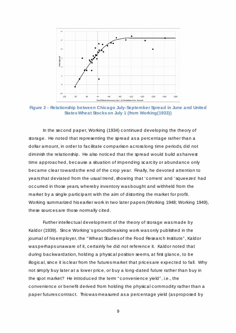
time there was abundance. Working plotted the July-September spread
(comparing pre- and post-harvest prices), as observed in June against the year-end
inventory, see Figure 2 (reproduced using Working’s original data), which we will
henceforth term the “Working curve”. A clear pattern emerged: in years of low
inventory, the prices of July futures were much higher than September futures,
resulting in a negative spread. In years with no shortage, September futures were
slightly more expensive, by an amount roughly equivalent to the additional cost of
storing wheat for two months. This result, showing that short-term futures rise in time
of scarcity, is Prediction 1. As well as this central result, Working also documented,
we believe for the first time, some other features of futures markets:
• Information affecting next year’s harvest (long term information) caused
equal change in prices for July and September, resulting in no changes in
spread. We would today term these as parallel shifts in the futures curve.
Conversely, short-term information, about this year’s harvest, affected short
term prices (July) more than long term prices (September).
• The average weekly changes in price of July wheat (what we would now
term volatility) varied more and more as harvest approached (the so-called
Samuelson (1965) effect).
• In situations of scarcity, when July wheat rose in price over September, its
volatility also rose greatly compared with situations of abundance (Prediction
2).
9
Figure 2 - Relationship between Chicago July-September Spread in June and United
States Wheat Stocks on July 1 (from Working(1933))
In the second paper, Working (1934) continued developing the theory of
storage. He noted that representing the spread as a percentage rather than a
dollar amount, in order to facilitate comparison across long time periods, did not
diminish the relationship. He also noticed that the spread would build as harvest
time approached, because a situation of impending scarcity or abundance only
became clear towards the end of the crop year. Finally, he devoted attention to
years that deviated from the usual trend, showing that ‘corners’ and ‘squeezes’ had
occurred in those years, whereby inventory was bought and withheld from the
market by a single participant with the aim of distorting the market for profit.
Working summarized his earlier work in two later papers (Working 1948; Working 1949),
these sources are those normally cited.
Further intellectual development of the theory of storage was made by
Kaldor (1939). Since Working’s groundbreaking work was only published in the
journal of his employer, the “Wheat Studies of the Food Research Institute”, Kaldor
was perhaps unaware of it, certainly he did not reference it. Kaldor noted that
during backwardation, holding a physical position seems, at first glance, to be
illogical, since it is clear from the futures market that prices are expected to fall. Why
not simply buy later at a lower price, or buy a long-dated future rather than buy in
the spot market? He introduced the term “convenience yield”, i.e., the
convenience or benefit derived from holding the physical commodity rather than a
paper futures contract. This was measured as a percentage yield (as proposed by
10
Working) which the holder of the physical asset implicitly receives to offset the
decline in price. Often the theory of storage is initially credited to Kaldor (Fama and
French 1987; Brennan 1958 and others). We believe that much belated credit is
mainly due to Working, partly because he ‘got there first’, and partly because
Working explicitly plots graphically the relationship between spread and inventory,
whereas Kaldor only discusses the relationship in general qualitative terms.
Brennan (1958) contributed further to the development of the theory of
storage. He took empirical data for a number of agricultural commodities (eggs,
cheese, butter, wheat and oats) over a period of years, and showed that the
Working curve was observed in many markets. Whereas Working had framed the
theory in terms of yearly observations, Brennan noted that it held at all times, using
monthly observations.
Further evidence to support the Working curve has been found over the years
in a range of commodities, such as heating oil, copper and lumber (Pindyck 1994),
soybeans (Geman and Nguyen 2005) and crude oil and natural gas (Geman and
Ohana 2009). Convenience yield is usually said not to exist in the case of electricity,
due to its non-storability. However, in the special case of the Scandinavian
Nordpool electricity market, unusual because a large proportion of its electricity is
generated from hydroelectric dams, water stored in the dams serves as an inventory
of electricity (Botterud, Kristiansen, and Ilic 2010). Watkins and McAleer (2006)
examine the LME base metals in an econometric sense, and find limited support for
a ‘cost of carry’ which is based on convenience yield and hence related to the
theory of storage.
1.2.4 Development of the Theory of Storage –Inventory and Volatility
The 2nd branch of the theory of storage, described in our Prediction 2 was
again first discussed by Working in his seminal 1933 paper. However, it took some
years before further empirical work was done on the relationship between volatility
and inventory.
Fama and French (1988) test five bases metals (aluminium, copper, lead, tin
and zinc) traded on the London Metal Exchange (LME) from 1972 to 1983, as well as
11
3 precious metals, gold, platinum and silver. In the absence of formal inventory data,
they use interested-adjusted spread as a proxy for inventory. In the case of the base
metals, they find that spot price volatility rises as inventory decreases. Gold
inventories are always high (central banks and other reserves hold inventory,
although the willingness of the owners to sell is sometimes in doubt), so spreads are
little-varying and therefore offer little forecast power for price volatility.
Other studies of the relationship between volatility and inventory in the case of
metals include:
• Ng and Pirrong (1994), who study four base metals traded on the London Metal
Exchange (LME): aluminium, copper, lead and zinc, from 1986-1992. They do not
have access to inventory information, so use the adjusted spread as a proxy.
They find, as predicted, a strong relationship between spread and spot price
volatility.
• Brunetti and Gilbert (1995) examine 6 LME-traded base metals and find that low
inventory levels (adjusted for worldwide consumption) are correlated with
periods of high spot price volatility.
12
2. Data and the Units of Inventory
The relationship between price and inventory is usually represented in terms of
convenience yield. The convenience yield, usually denoted ( , )y t T , the benefit
accruing to a holder of a physical commodity between times t and T that is not
enjoyed by the owner of a futures contract , can be derived from the spot-futures
relationship in Equation (1) (See Appendix 1 for details).
[ ( , ) ( , ) ( , )]( )( , ) ( ) r t T c t T y t T T tF t T S t e + − −= (1)
We therefore need a historical database of prices, both spot and futures for
the 6 base metals, as well as of ( , )r t T , the cost of financing over ( , )t T in the
currency in which the commodity is traded, and ( , )c t T , storage costs per unit of
inventory from time t to T . Naturally we also need a historical database recording
the quantity of each metal held in inventory.
2.1 Price Database
In many commodity markets, liquidity exists mainly in the futures market while
spot markets are thinly traded, if at all. In these cases, it is common to use the first
nearby future price as a proxy for the spot price. Still, futures prices often suffer from
technicalities around rollover dates and thin liquidity as delivery date approaches.
Fortunately, structural reasons related to the nature of trading imply that metal spot
and futures prices reported by the LME are reliable and can be used directly (Fama
and French 1988). Since the theory of storage is mainly concerned with relatively
short-term effects caused by abundant or low inventory, we study the ‘short’ end of
the futures curve using the spot and 3 month prices published by the LME.
Our price database from the LME covers the period January 1983 to June
2011, except in the case of tin and zinc, when we start in January 1990 due to
absence of inventory data or suspension of trading during the earlier period. All
prices were initially quoted in British Pounds during the early years of our study period,
later transferring into US$, so when necessary we convert to US$ using the prevailing
spot £/$ spot rates.
13
2.2 Inventory Database
We mainly use inventory data as reported daily by the LME, being the total
metal inventory held in the large number of LME-appointed warehouses worldwide.
All inventory figures are in metric tonnes. We also compiled additional inventory
data:
• Aluminium and Copper also trade (or were traded) for some years on the
COMEX exchange in New York, although the main world market remains the LME.
COMEX publishes its own daily inventory data for its warehouses.
• The US Geographical Survey (USGS) publishes its estimates of annual, year-end US
commercial stocks for all 6 base metals. However, in some cases, there is risk of
double-counting inventory held in US-based LME warehouses.
• In recent years, the Shanghai Futures Exchange, SHFE, has begun trading
aluminium, copper and zinc and publishes its own daily warehouse figures from
2003 onwards (2007 for zinc).
• In the case of Aluminium, the International Aluminium Institute publishes results of
monthly surveys of worldwide total zinc commercial and government stocks, and
explicitly excludes LME warehouses.
2.3 World Consumption Database
In order to compare inventory with increasing worldwide consumption, we
use an annual series of worldwide metal consumption (this includes both primary
and secondary – recycled – materials), from World Metal Statistics.
2.4 Storage Costs
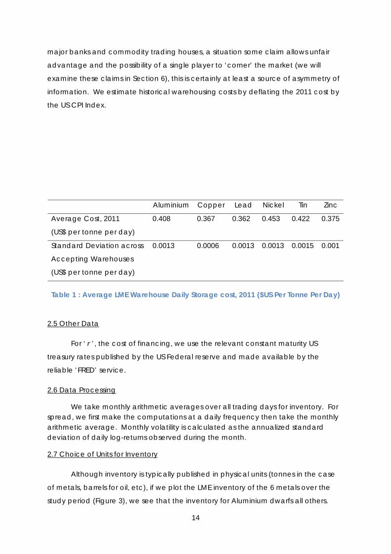
Historical storage costs are unavailable for the LME warehouses. At the time
of writing, 2011, costs for all six of the base metals, at all warehouses worldwide, were
in the range $0.36 - $0.46 per tonne per day (LME 2011b), summarized in Table 1.
These costs are typically set once per year, with minimal variations from year to year.
The costs correspond to annual storage costs ranging from <1% to 5% p.a. of the
value of the metal, i.e. low numbers compared to the situation of crude oil or natural
gas. Warehouse costs are highly consistent across the globe (see the low standard
deviations of cost across all relevant warehouses in Table 1). There are few
warehouse operators, and in recent years they have mainly been taken over by the
14
major banks and commodity trading houses, a situation some claim allows unfair
advantage and the possibility of a single player to ‘corner’ the market (we will
examine these claims in Section 6), this is certainly at least a source of asymmetry of
information. We estimate historical warehousing costs by deflating the 2011 cost by
the US CPI Index.
Aluminium Copper Lead Nickel Tin Zinc
Average Cost, 2011
(US$ per tonne per day)
0.408 0.367 0.362 0.453 0.422 0.375
Standard Deviation across
Accepting Warehouses
(US$ per tonne per day)
0.0013 0.0006 0.0013 0.0013 0.0015 0.001
Table 1 : Average LME Warehouse Daily Storage cost, 2011 ($US Per Tonne Per Day)
2.5 Other Data
For ‘ r ’, the cost of financing, we use the relevant constant maturity US
treasury rates published by the US Federal reserve and made available by the
reliable ‘FRED’ service.
2.6 Data Processing
We take monthly arithmetic averages over all trading days for inventory. For spread, we first make the computations at a daily frequency then take the monthly arithmetic average. Monthly volatility is calculated as the annualized standard deviation of daily log-returns observed during the month.
2.7 Choice of Units for Inventory
Although inventory is typically published in physical units (tonnes in the case
of metals, barrels for oil, etc), if we plot the LME inventory of the 6 metals over the
study period (Figure 3), we see that the inventory for Aluminium dwarfs all others.
15
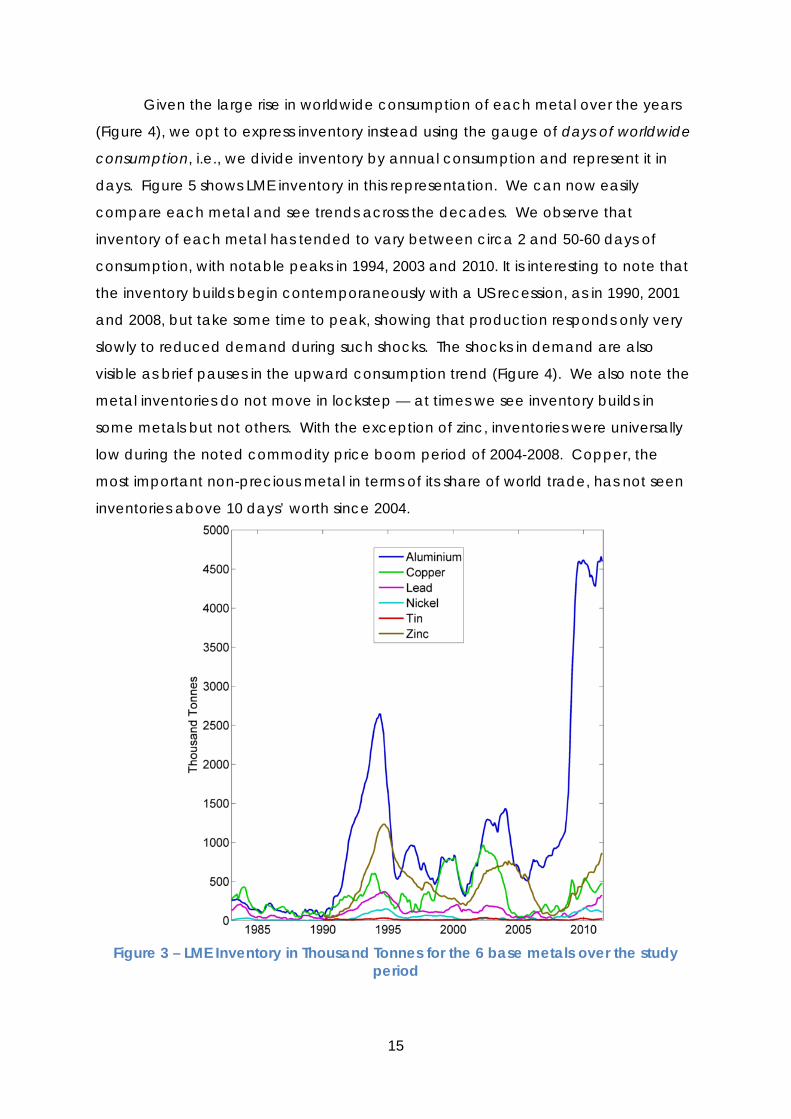
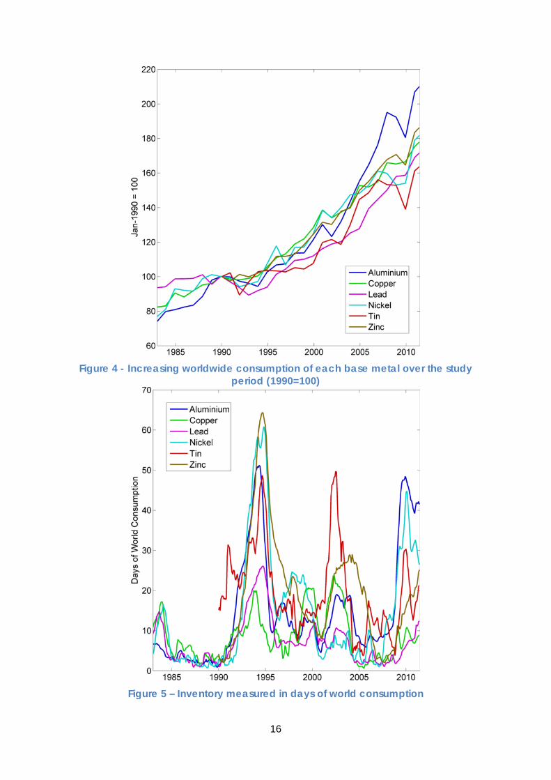
Given the large rise in worldwide consumption of each metal over the years
(Figure 4), we opt to express inventory instead using the gauge of days of worldwide
consumption, i.e., we divide inventory by annual consumption and represent it in
days. Figure 5 shows LME inventory in this representation. We can now easily
compare each metal and see trends across the decades. We observe that
inventory of each metal has tended to vary between circa 2 and 50-60 days of
consumption, with notable peaks in 1994, 2003 and 2010. It is interesting to note that
the inventory builds begin contemporaneously with a US recession, as in 1990, 2001
and 2008, but take some time to peak, showing that production responds only very
slowly to reduced demand during such shocks. The shocks in demand are also
visible as brief pauses in the upward consumption trend (Figure 4). We also note the
metal inventories do not move in lockstep — at times we see inventory builds in
some metals but not others. With the exception of zinc, inventories were universally
low during the noted commodity price boom period of 2004-2008. Copper, the
most important non-precious metal in terms of its share of world trade, has not seen
inventories above 10 days’ worth since 2004.
Figure 3 – LME Inventory in Thousand Tonnes for the 6 base metals over the study
period
16
Figure 4 - Increasing worldwide consumption of each base metal over the study
period (1990=100)
Figure 5 – Inventory measured in days of world consumption
17
3. Results : The Relationship between Price and Inventory
As in Working (1933) we represent the relationship between spot and futures
prices in terms of a spread, rather than looking at convenience yield. More precisely,
we follow Geman and Ohana (2009) and others by calculating an ‘interest and
storage adjusted spread’
[ ( , ) ( , )]( )( , ) ( )( , )
( )
r t T c t T T tF t T S t et TS t
ψ+ −−
= (2)
i.e., it is a ratio, representing the growth from the current spot price ( )S t to the futures
price ( , )F t T for maturity T t> , adjusted for financing and storage costs. As a ratio, it
can be thought of as a return relative to ( )S t from holding the physical commodity
between t and T , and selling one future contract at date t for delivery at T .
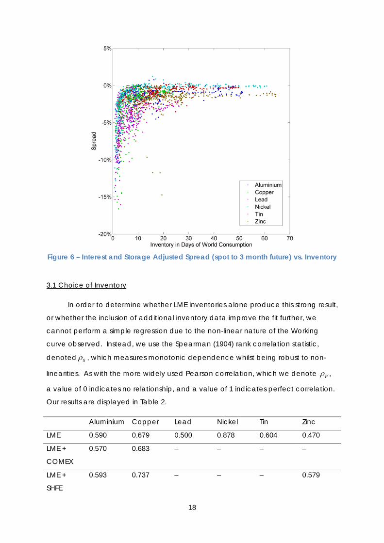
In Figure 6, we plot, for each metal, a scattergram of monthly observations of
the interest and storage adjusted spread (henceforth, ‘spread’) ( , )t Tψ against its
contemporaneous inventory ( )i t . A very clear and consistent picture emerges,
relatively identical for each metal. We note the following features:
1. The vertical axis represents the extent to which the spot price is below the futures
price, after funding and storage costs are removed. That is, a negative spread
represents backwardation, with spot > futures.
2. The spread almost never exceeds 0, as expected; otherwise this would represent
an arbitrage opportunity, obtained by purchasing the spot asset and
simultaneously selling a 3 month future, paying funding and storage costs for 3
months, and delivering the metal to the futures counterparty after 3 months.
3. Whenever inventory exceeds around 30 days of worldwide consumption, we see
a negligible spread, i.e., the futures curve is neither in strong backwardation nor
contango.
4. When inventory falls below 10 days of worldwide consumption, an extreme
spread often occurs, with spot 5% or even 10% above 3 month futures.
5. The curve is exactly as Working observed for wheat. However, he expressed
inventory in terms of ‘variation from the usual’ whereas we measured absolute
inventory in days of worldwide consumption.
18
Figure 6 – Interest and Storage Adjusted Spread (spot to 3 month future) vs. Inventory
3.1 Choice of Inventory
In order to determine whether LME inventories alone produce this strong result,
or whether the inclusion of additional inventory data improve the fit further, we
cannot perform a simple regression due to the non-linear nature of the Working
curve observed. Instead, we use the Spearman (1904) rank correlation statistic,
denoted Sρ , which measures monotonic dependence whilst being robust to non-
linearities. As with the more widely used Pearson correlation, which we denote Pρ ,
a value of 0 indicates no relationship, and a value of 1 indicates perfect correlation.
Our results are displayed in Table 2.
Aluminium Copper Lead Nickel Tin Zinc
LME 0.590 0.679 0.500 0.878 0.604 0.470
LME +
COMEX
0.570 0.683 – – – –
LME +
SHFE
0.593 0.737 – – – 0.579
19
LME +
COMEX +
SHFE
0.578 0.731 – – – 0.579
LME +
USGS
0.271 0.660 0.253 0.597 0.518 0.168
LME+IAI 0.100 – – – – –
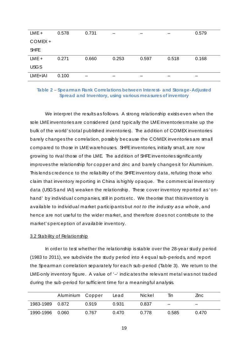
Table 2 – Spearman Rank Correlations between Interest- and Storage-Adjusted
Spread and Inventory, using various measures of inventory
We interpret the results as follows. A strong relationship exists even when the
sole LME inventories are considered (and typically the LME inventories make up the
bulk of the world’s total published inventories). The addition of COMEX inventories
barely changes the correlation, possibly because the COMEX inventories are small
compared to those in LME warehouses. SHFE inventories, initially small, are now
growing to rival those of the LME. The addition of SHFE inventories significantly
improves the relationship for copper and zinc and barely changes it for Aluminium.
This lends credence to the reliability of the SHFE inventory data, refuting those who
claim that inventory reporting in China is highly opaque. The commercial inventory
data (USGS and IAI) weaken the relationship. These cover inventory reported as ‘on-
hand’ by individual companies, still in ports etc. We theorise that this inventory is
available to individual market participants but not to the industry as a whole, and
hence are not useful to the wider market, and therefore does not contribute to the
market’s perception of available inventory.
3.2 Stability of Relationship
In order to test whether the relationship is stable over the 28-year study period
(1983 to 2011), we subdivide the study period into 4 equal sub-periods, and report
the Spearman correlation separately for each sub-period (Table 3). We return to the
LME-only inventory figure. A value of ‘–‘ indicates the relevant metal was not traded
during the sub-period for sufficient time for a meaningful analysis.
Aluminium Copper Lead Nickel Tin Zinc
1983-1989 0.872 0.919 0.931 0.837 – –
1990-1996 0.060 0.767 0.470 0.778 0.585 0.470
20
1997-2003 0.11 0.790 0.160 0.809 0.812 0.319
2004-2011 0.627 0.914 0.578 0.850 0.507 0.284
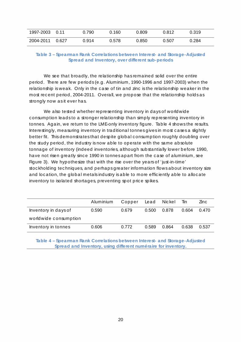
Table 3 – Spearman Rank Correlations between Interest- and Storage-Adjusted
Spread and Inventory, over different sub-periods
We see that broadly, the relationship has remained solid over the entire period. There are few periods (e.g. Aluminium, 1990-1996 and 1997-2003) when the relationship is weak. Only in the case of tin and zinc is the relationship weaker in the most recent period, 2004-2011. Overall, we propose that the relationship holds as strongly now as it ever has.
We also tested whether representing inventory in days of worldwide consumption leads to a stronger relationship than simply representing inventory in tonnes. Again, we return to the LME-only inventory figure. Table 4 shows the results. Interestingly, measuring inventory in traditional tonnes gives in most cases a slightly better fit. This demonstrates that despite global consumption roughly doubling over the study period, the industry is now able to operate with the same absolute tonnage of inventory (indeed inventories, although substantially lower before 1990, have not risen greatly since 1990 in tonnes apart from the case of aluminium, see Figure 3). We hypothesize that with the rise over the years of ‘just-in-time’ stockholding techniques, and perhaps greater information flows about inventory size and location, the global metals industry is able to more efficiently able to allocate inventory to isolated shortages, preventing spot price spikes.
Aluminium Copper Lead Nickel Tin Zinc
Inventory in days of
worldwide consumption
0.590 0.679 0.500 0.878 0.604 0.470
Inventory in tonnes 0.606 0.772 0.589 0.864 0.638 0.537
Table 4 – Spearman Rank Correlations between Interest- and Storage-Adjusted
Spread and Inventory, using different numéraire for inventory.
21
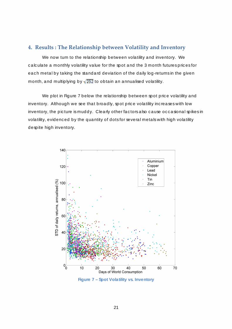
4. Results : The Relationship between Volatility and Inventory
We now turn to the relationship between volatility and inventory. We
calculate a monthly volatility value for the spot and the 3 month futures prices for
each metal by taking the standard deviation of the daily log-returns in the given
month, and multiplying by to obtain an annualised volatility.
We plot in Figure 7 below the relationship between spot price volatility and
inventory. Although we see that broadly, spot price volatility increases with low
inventory, the picture is muddy. Clearly other factors also cause occasional spikes in
volatility, evidenced by the quantity of dots for several metals with high volatility
despite high inventory.
Figure 7 – Spot Volatility vs. Inventory
22
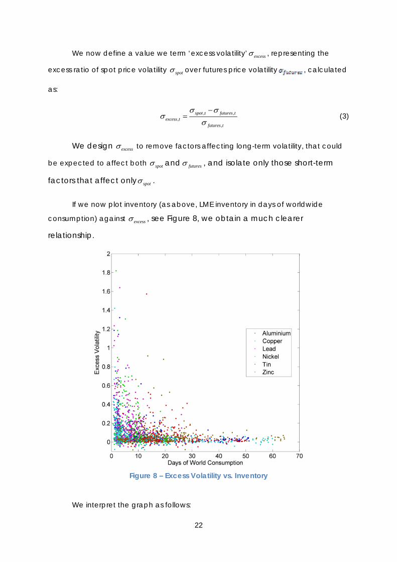
We now define a value we term ‘excess volatility’ excessσ , representing the
excess ratio of spot price volatility spotσ over futures price volatility , calculated
as:
, ,,
,
spot t futures texcess t
futures t
σ σσ
σ−
= (3)
We design excessσ to remove factors affecting long-term volatility, that could
be expected to affect both spotσ and futuresσ , and isolate only those short-term
factors that affect only spotσ .
If we now plot inventory (as above, LME inventory in days of worldwide
consumption) against excessσ , see Figure 8, we obtain a much clearer
relationship.
Figure 8 – Excess Volatility vs. Inventory
We interpret the graph as follows:
23
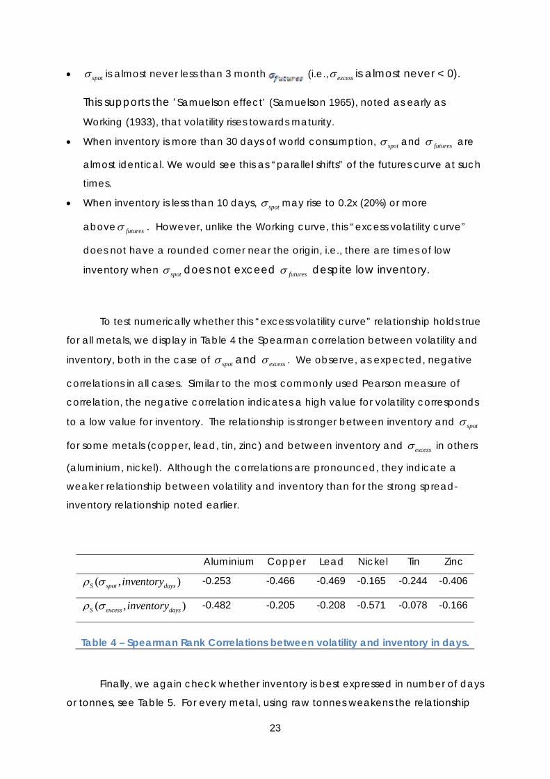
• spotσ is almost never less than 3 month (i.e., excessσ is almost never < 0).
This supports the ‘Samuelson effect’ (Samuelson 1965), noted as early as
Working (1933), that volatility rises towards maturity.
• When inventory is more than 30 days of world consumption, spotσ and futuresσ are
almost identical. We would see this as “parallel shifts” of the futures curve at such
times.
• When inventory is less than 10 days, spotσ may rise to 0.2x (20%) or more
above futuresσ . However, unlike the Working curve, this “excess volatility curve”
does not have a rounded corner near the origin, i.e., there are times of low
inventory when spotσ does not exceed futuresσ despite low inventory.
To test numerically whether this “excess volatility curve” relationship holds true
for all metals, we display in Table 4 the Spearman correlation between volatility and
inventory, both in the case of spotσ and excessσ . We observe, as expected, negative
correlations in all cases. Similar to the most commonly used Pearson measure of
correlation, the negative correlation indicates a high value for volatility corresponds
to a low value for inventory. The relationship is stronger between inventory and spotσ
for some metals (copper, lead, tin, zinc) and between inventory and excessσ in others
(aluminium, nickel). Although the correlations are pronounced, they indicate a
weaker relationship between volatility and inventory than for the strong spread-
inventory relationship noted earlier.
Aluminium Copper Lead Nickel Tin Zinc
( , )S spot daysinventoryρ σ -0.253 -0.466 -0.469 -0.165 -0.244 -0.406
( , )S excess daysinventoryρ σ -0.482 -0.205 -0.208 -0.571 -0.078 -0.166
Table 4 – Spearman Rank Correlations between volatility and inventory in days.
Finally, we again check whether inventory is best expressed in number of days
or tonnes, see Table 5. For every metal, using raw tonnes weakens the relationship
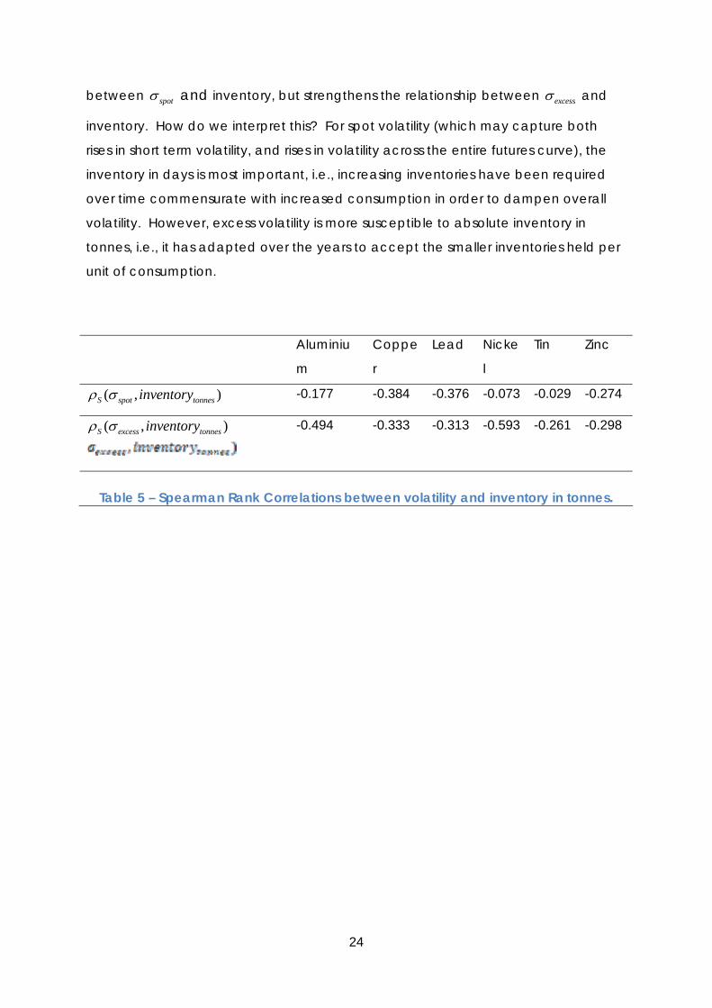
24
between spotσ and inventory, but strengthens the relationship between excessσ and
inventory. How do we interpret this? For spot volatility (which may capture both
rises in short term volatility, and rises in volatility across the entire futures curve), the
inventory in days is most important, i.e., increasing inventories have been required
over time commensurate with increased consumption in order to dampen overall
volatility. However, excess volatility is more susceptible to absolute inventory in
tonnes, i.e., it has adapted over the years to accept the smaller inventories held per
unit of consumption.
Aluminiu
m
Coppe
r
Lead Nicke
l
Tin Zinc
( , )S spot tonnesinventoryρ σ -0.177 -0.384 -0.376 -0.073 -0.029 -0.274
( , )S excess tonnesinventoryρ σ
-0.494 -0.333 -0.313 -0.593 -0.261 -0.298
Table 5 – Spearman Rank Correlations between volatility and inventory in tonnes.
25
5. Applications
We see several applications for these results, detailed below.
5.1 Forecasting
Trajectories of inventory, as demonstrated in Figures 3 and 5, appear to be
mean-reverting, and are certainly not random walks. They display high levels of
autocorrelation in their changes, i.e., inventory rises or falls continuously for many
weeks before reverting. Over the short term of several weeks, inventory changes are
therefore fairly predictable. Given the strong influence of inventory over both the
spot-futures price spread and various measures of volatility, a model for inventory
could thereby predict likely spreads and volatilities out to an horizon of perhaps 1 or
2 months. We propose that the use of stochastic differential equations with
autocorrelation of returns and mean-reversion of levels would be a good starting
point for modelling base metal inventories.
5.2 Investigating Market Abnormalities
The seminal paper of Black and Scholes (1973) showed that given several
parameters, namely the price of an underlying asset and its volatility, the risk free
interest rate, and a duration, the value of an option contingent on that asset could
be expressed as a simple closed-form formula. It was soon observed that given an
option price already quoted in the market, and the other parameters excluding
volatility, an implied volatility could be calculated, namely the (unique) volatility that
would give that option price had the Black-Scholes option pricing formula been
used. This implied volatility can in turn be used to price more complex options, or it
can be used to confirm that the various options on an underlying are neither under-
or over-priced.
We propose a similar approach; we derive inventory implied spot price and
inventory implied spot volatility for a commodity. We can compare these with
observed values of spot price and spot price volatility. If the implied and market
values are in agreement, we can conclude that the market is functioning “normally”
with respect to inventory, i.e., the inventory in warehouses is considered “useful” to
26
the market in the normal way. If inventory has been “cornered” by a market
participant, or another market abnormality implies that inventory is not “available”
to the wider market, we would expect to see elevated values for spot price and
spot price volatility.
5.3 Inventory Implied Spot Price
We fit a functional form between spread and inventory, as plotted in Figure 6.
We choose for the functional form:
( )( , ) Bi tt T Ae Cψ = + (4)
where we expect 0A < , 0B < , 0C ≈ with 0C ≤ reflecting no cash-and-carry
arbitrage opportunities, and 3T t= + months as in the rest of our analysis. Rather
than calibrate using simple least-square methodology, which fits the curve based on
the bulk of the observations and are of moderate inventory values in each case, we
employ a variation of least-squares described in Appendix 2.
Others have fitted different functional forms to the relationship between
inventory and spread to convert it to a linear one. Geman and Nguyen (2005) used
1 , 0( )
K Ki t
< (5)
for soybeans, where scarcity is defined as inverse inventory, and obtain conclusive
results.
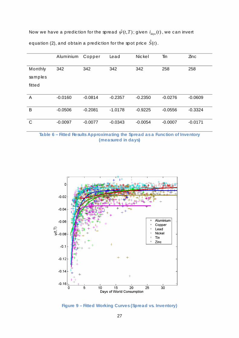
We displayed the results for each metal in Table 6, and the fitted curves in
Figure 9. We note that the fitted curves take a similar form for each metal, although
copper displays a ‘tighter’ curve (indicating tolerance of lower inventory values than
for other metals) and tin displays little curvature. In the case of tin, we have never
had a case of extremely low inventories, so there are no ‘low inventory’ values to fit
and the fitted line does not curve sharply downwards.
27
Now we have a prediction for the spread ˆ ( , )t Tψ ; given ( )daysi t , we can invert
equation (2), and obtain a prediction for the spot price ˆ( )S t .
Aluminium Copper Lead Nickel Tin Zinc
Monthly
samples
fitted
342 342 342 342 258 258
A -0.0160 -0.0814 -0.2357 -0.2350 -0.0276 -0.0609
B -0.0506 -0.2081 -1.0178 -0.9225 -0.0556 -0.3324
C -0.0097 -0.0077 -0.0343 -0.0054 -0.0007 -0.0171
Table 6 – Fitted Results Approximating the Spread as a Function of Inventory (measured in days)
Figure 9 – Fitted Working Curves (Spread vs. Inventory)
28
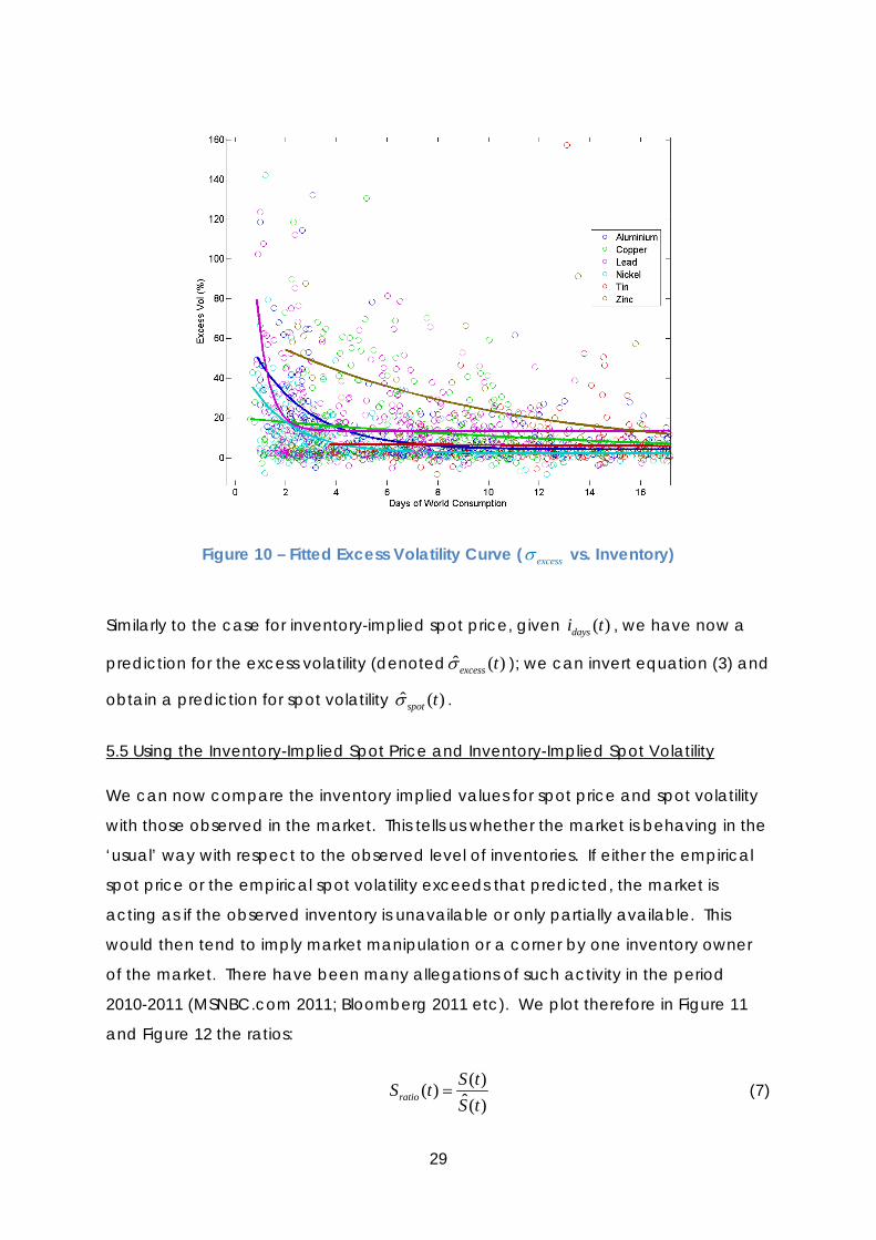
5.4 Inventory Implied Spot Volatility
Noting from Figure 8 the similar form of the relationship between inventory and
excess volatility excessσ (defined in equation(3)), we repeat the above exercise, fitting
a curve of the same form:
( )( ) Bi texcess t Ae Cσ = + (6)
Where again now expect 0A > , 0B < , 0C ≈ but not necessarily 0C > because
there is no economic reason to anticipate spotσ to be always higher than futures. A
fitted graph is displayed in Figure 10 and the fitted values in Table 11. The fitted
curves all take the same form, although again the tin ‘curve’ has little curvature due
to the lack of low-inventory historical values for tin. We also see surprisingly little
curvature for copper.
Aluminium Copper Lead Nickel Tin Zinc
Weekly
samples
to fit
342 342 342 342 258 258
A 0.6882 0.1984 3.8888 0.4979 0.0627 0.6534
B -0.4540 -0.0636 -2.0678 -0.5839 -0.0109 -0.1087
C 0.0422 0.0047 0.1351 0.0237 0.0080 0.0189
Table 11 - Fitted Results Approximating the ‘Excess Volatility’ as a Function of Inventory (measured in days)
29
Figure 10 – Fitted Excess Volatility Curve ( excessσ vs. Inventory)
Similarly to the case for inventory-implied spot price, given ( )daysi t , we have now a
prediction for the excess volatility (denoted ˆ ( )excess tσ ); we can invert equation (3) and
obtain a prediction for spot volatility ( )ˆ spot tσ .
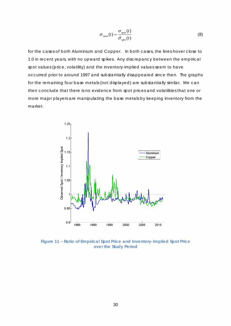
5.5 Using the Inventory-Implied Spot Price and Inventory-Implied Spot Volatility
We can now compare the inventory implied values for spot price and spot volatility
with those observed in the market. This tells us whether the market is behaving in the
‘usual’ way with respect to the observed level of inventories. If either the empirical
spot price or the empirical spot volatility exceeds that predicted, the market is
acting as if the observed inventory is unavailable or only partially available. This
would then tend to imply market manipulation or a corner by one inventory owner
of the market. There have been many allegations of such activity in the period
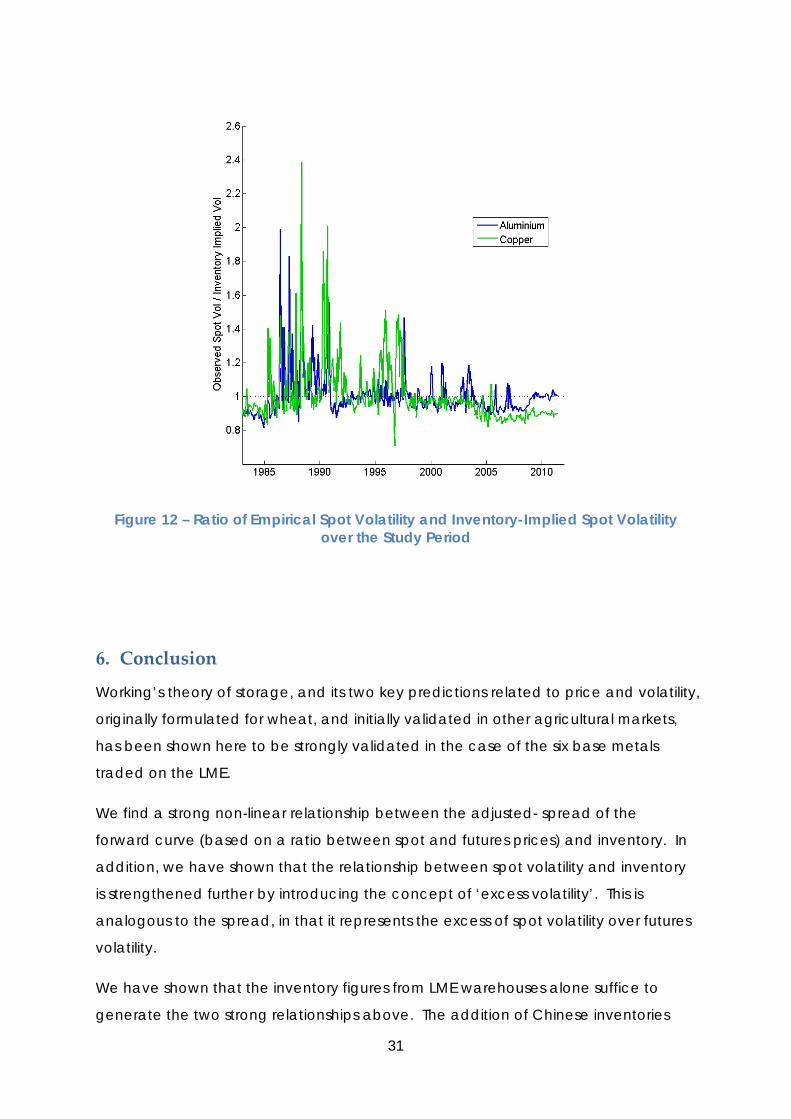
2010-2011 (MSNBC.com 2011; Bloomberg 2011 etc). We plot therefore in Figure 11
and Figure 12 the ratios:
( )( ) ˆ( )ratio
S tS tS t
= (7)
30
( )
( )ˆ ( )
spotratio
spot
tt
tσ
σσ
= (8)
for the cases of both Aluminium and Copper. In both cases, the lines hover close to
1.0 in recent years, with no upward spikes. Any discrepancy between the empirical
spot values (price, volatility) and the inventory-implied values seem to have
occurred prior to around 1997 and substantially disappeared since then. The graphs
for the remaining four base metals (not displayed) are substantially similar. We can
then conclude that there is no evidence from spot prices and volatilities that one or
more major players are manipulating the base metals by keeping inventory from the
market.
Figure 11 – Ratio of Empirical Spot Price and Inventory-Implied Spot Price
over the Study Period
31
Figure 12 – Ratio of Empirical Spot Volatility and Inventory-Implied Spot Volatility
over the Study Period
6. Conclusion
Working’s theory of storage, and its two key predictions related to price and volatility,
originally formulated for wheat, and initially validated in other agricultural markets,
has been shown here to be strongly validated in the case of the six base metals
traded on the LME.
We find a strong non-linear relationship between the adjusted- spread of the
forward curve (based on a ratio between spot and futures prices) and inventory. In
addition, we have shown that the relationship between spot volatility and inventory
is strengthened further by introducing the concept of ‘excess volatility’. This is
analogous to the spread, in that it represents the excess of spot volatility over futures
volatility.
We have shown that the inventory figures from LME warehouses alone suffice to
generate the two strong relationships above. The addition of Chinese inventories
32
figures at the SHFE slightly strengthens the relationship further, highlighting the
increasing importance of China in metal demand and trade, and refuting some
suggestions that Chinese inventory data cannot be trusted. The addition of
inventory figures from other exchanges and trade organisations does not improve
the relationship, highlighting further that only the LME and the SHFE need be
followed, for now at least.
Finally, based on our novel concepts of inventory-implied spot price and inventory-
implied spot volatility, we seen no evidence that the recent allegations of major
market players withholding inventory is substantiated, to the extent that LME prices
are behaving as if the full inventory figures are available to the market.
Acknowledgements
The authors wish to thank Prof. Chris Gilbert for assistance with obtaining historical
data, and the participants of the London Graduate School in Mathematical Finance
Symposium 2011 for their helpful comments. William O. Smith gratefully
acknowledges the receipt of a research studentship from Birkbeck College, London.
33
Appendix A – The Calculation of Convenience Yield and Interest‐
Adjusted Spread
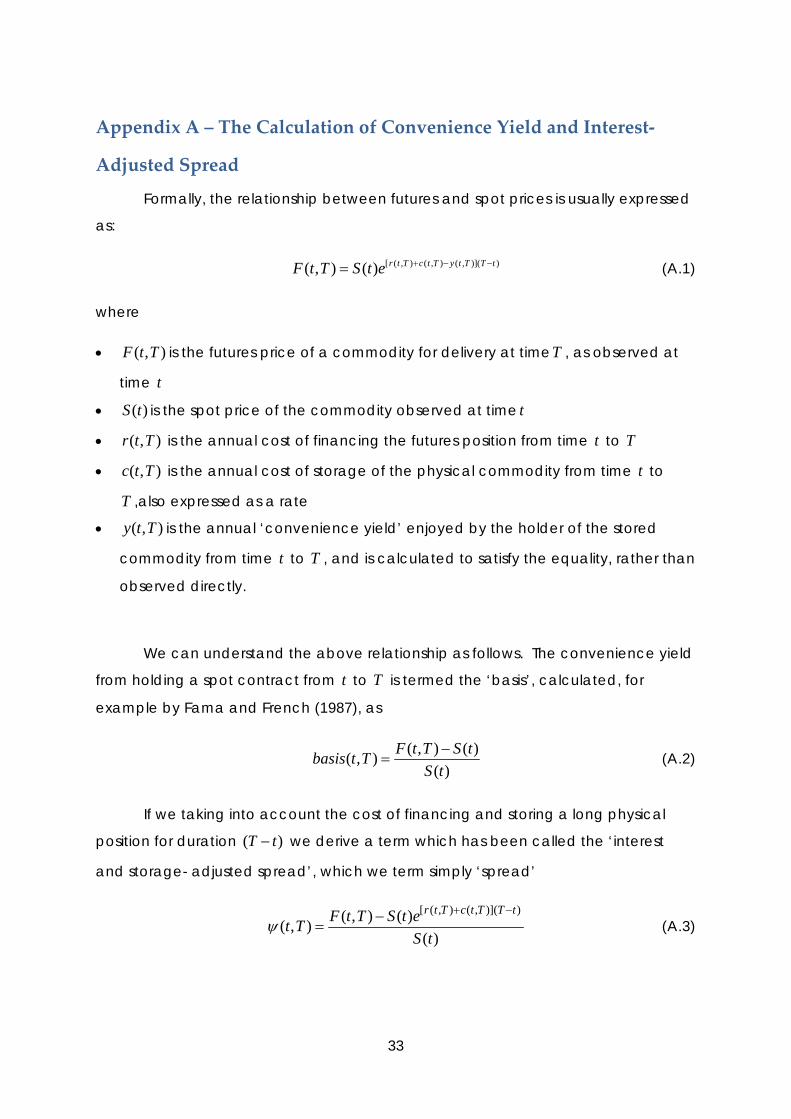
Formally, the relationship between futures and spot prices is usually expressed
as:
[ ( , ) ( , ) ( , )]( )( , ) ( ) r t T c t T y t T T tF t T S t e + − −= (A.1)
where
• ( , )F t T is the futures price of a commodity for delivery at timeT , as observed at
time t
• ( )S t is the spot price of the commodity observed at time t
• ( , )r t T is the annual cost of financing the futures position from time t to T
• ( , )c t T is the annual cost of storage of the physical commodity from time t to
T ,also expressed as a rate
• ( , )y t T is the annual ‘convenience yield’ enjoyed by the holder of the stored
commodity from time t to T , and is calculated to satisfy the equality, rather than
observed directly.
We can understand the above relationship as follows. The convenience yield
from holding a spot contract from t to T is termed the ‘basis’, calculated, for
example by Fama and French (1987), as
( , ) ( )( , )
( )F t T S tbasis t T
S t−
= (A.2)
If we taking into account the cost of financing and storing a long physical
position for duration ( )T t− we derive a term which has been called the ‘interest
and storage- adjusted spread’, which we term simply ‘spread’
[ ( , ) ( , )]( )( , ) ( )( , )( )
r t T c t T T tF t T S t et TS t
ψ+ −−
= (A.3)
34
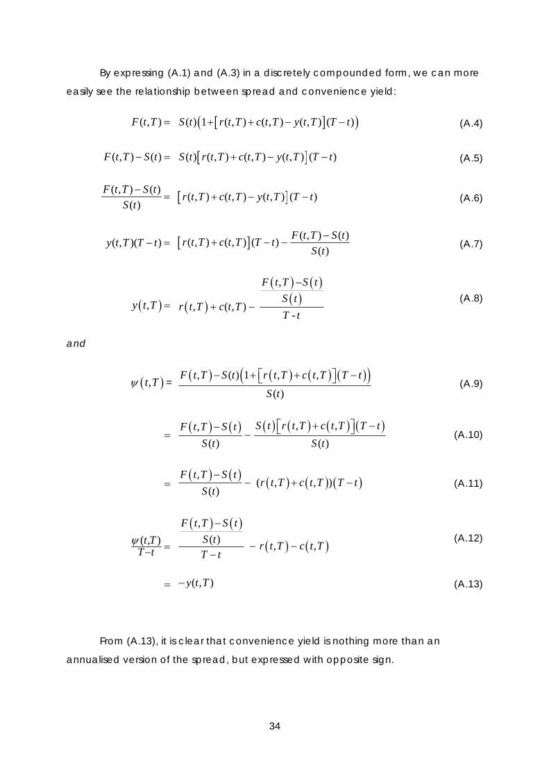
By expressing (A.1) and (A.3) in a discretely compounded form, we can more
easily see the relationship between spread and convenience yield:
( , )F t T = [ ]( )( ) 1 ( , ) ( , ) ( , ) ( )S t r t T c t T y t T T t+ + − − (A.4)
( , ) ( )F t T S t− = [ ]( ) ( , ) ( , ) ( , ) ( )S t r t T c t T y t T T t+ − − (A.5)
( , ) ( )( )
F t T S tS t−
= [ ]( , ) ( , ) ( , ) ( )r t T c t T y t T T t+ − − (A.6)
( , )( )y t T T t− = [ ] ( , ) ( )( , ) ( , ) ( )( )
F t T S tr t T c t T T tS t−
+ − − (A.7)
( ),y t T =
( )
( ) ( )( )
, –
, ( , )-
F t T S tS t
r t T c t TT t
+ − (A.8)
and
( ),t Tψ = ( ) ( ) ( ) ( )( ), ( ) 1 , ,
( )
F t T S t r t T c t T T t
S t
⎡ ⎤− + + −⎣ ⎦ (A.9)
= ( ) ( ) ( ) ( ) ( ) ( ), ,,
( ) ( )
S t r t T c t T T tF t T S tS t S t
⎡ ⎤+ −− ⎣ ⎦− (A.10)
= ( ) ( ) ( ) ( ) ( ),
( , , )( )
F t T S tr t T c t T T t
S t−
− + − (A.11)
( , )t TT t
ψ =−
( ) ( )
( ) ( )
, ( ) , ,
F t T S tS t r t T c t TT t
−
− −−
(A.12)
= ( , )y t T− (A.13)
From (A.13), it is clear that convenience yield is nothing more than an
annualised version of the spread, but expressed with opposite sign.
35
Appendix B – Exponential Curve Fitting Procedure
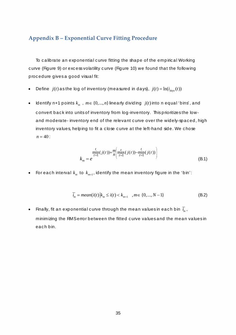
To calibrate an exponential curve fitting the shape of the empirical Working
curve (Figure 9) or excess volatility curve (Figure 10) we found that the following
procedure gives a good visual fit:
• Define ( )j t as the log of inventory (measured in days), ( ) ln( ( ))daysj t i t=
• Identify n+1 points mk , {0,..., }m n∈ linearly dividing ( )j t into n equal ‘bins’, and
convert back into units of inventory from log-inventory. This prioritizes the low-
and moderate- inventory end of the relevant curve over the widely-spaced, high
inventory values, helping to fit a close curve at the left-hand side. We chose
40n = :
1 11
min( ( )) max( ( )) min( ( ))
m
t ttmj j jnk e
τ τττ τ τ
⎛ ⎞⎜ ⎟⎜ ⎟⎜ ⎟⎝ ⎠
= ==+ −
= (B.1)
• For each interval mk to 1mk + , identify the mean inventory figure in the ‘bin’:
1( ( ) ( ) , {0,..., 1}m m mi mean i t k i t k m N+= ≤ < ∈ − (B.2)
• Finally, fit an exponential curve through the mean values in each bin mi ,
minimizing the RMS error between the fitted curve values and the mean values in
each bin.
36
References
Black, F., Scholes, M., 1973. The Pricing of Options and Corporate Liabilities. The J. of Political Econ. 81 (3), 637–654.
Bloomberg, 2011. Seven-Month Wait for Aluminum Drives LME to Review Rules - Bloomberg. http://www.bloomberg.com/news/2011-07-13/seven-month-wait-for-aluminum-from-detroit-drives-lme-to-review-warehouses.html
Botterud, A., Kristiansen, T., Ilic, M.D., 2010. The relationship between spot and futures prices in the Nord Pool electricity market. Energy Econ. 32 (5), 967-978.
Brennan, M.J, 1958. The Supply of Storage. The Am. Econ. Rev. 48 (1), 50-72. Brunetti, C., Gilbert, C.L., 1995. Metals Price Volatility, 1972-1995. Resour. Policy
21 (4), 237–254. Fama, E. F., French, K.R., 1987. Commodity futures prices: Some evidence on
forecast power, premiums, and the theory of storage. J. of Bus. 60 (1), 55-73.
Fama, F., French, K.R, 1988. Business Cycles and the Behavior of Metals Prices. The J. of Finance 43 (5), 1075–1093.
Geman, H., Ohana, S., 2009. Forward curves, scarcity and price volatility in oil and natural gas markets. Energy Econ. 31 (4), 576-585.
Geman, H., Nguyen, V.-N., 2005. Soybean Inventory and Forward Curve Dynamics. Manag. Sci. 51 (7), 1076-1091.
Johnston, B.F., 1996. The History of the Food Research Institute as Seen Through Its Publications: a Long View. http://www.stanford.edu/group/FRI/fri/history/bfjohn.fm.html.
Kaldor, N., 1939. Speculation and Economic Stability. The Rev. of Econ. Stud. 1, 1–27.
Keynes, J.M., 1930. A Treatise on Money. Harcourt, Brace and Company, New York.
LME, 2011a. Ring Trading. http://www.lme.com/who_how_ringtrading.asp. ———. 2011b. Warehousing & Delivery.
http://www.lme.com/warehousing.asp. MSNBC.com, 2011. Goldman’s New Money Machine: Warehouses.
http://www.msnbc.msn.com/id/43931226/ns/business-us_business/#.ToNE9Owt1Bk.
Ng, V.K., Pirrong, S.C., 1994. Fundamentals and Volatility: Storage, Spreads, and the Dynamics of Metals Prices. The J. of Bus. 67 (2), 203-230.
Pindyck, R.S., 1994. Inventories and the Short-Run Dynamics of Commodity Prices. The RAND J. of Econ. 25 (1), 141-159.
Samuelson, P.A., 1965. Proof That Properly Anticipated Prices Fluctuate Randomly. Ind. Manag. Rev. 6, 41–49.
Spearman, C., 1904. The Proof and Measurement of Association Between Two Things. The Am. J. of Psychol. 15, 72–101.
37
Watkins, C., McAleer, M., 2006. Pricing of Non-ferrous Metals Futures on the London Metal Exchange. Appl. Financial Econ. 16 (12), 853-880.
Working, H., 1927. Forecasting the Price of Wheat. J. of Farm Econ. 9 (3), 273–287.
———. 1933. Price Relations between July and September Wheat Futures at Chicago Since 1885. Wheat Stud. of the Food Res. Inst. 9 (6).
———. 1934. Price Relations Between May and New-Crop Wheat Futures at Chicago Since 1885. Wheat Stud. of the Food Res. Inst. 10 (5).
———. 1948. Theory of the Inverse Carrying Charge in Futures Markets. J. of Farm Econ. 30 (1), 1-28.
———. 1949. ‘The Theory of Price of Storage’. The Am. Econ. Rev. 39 (6), 1254–1262.