This page has been reformatted by Knovel to provide easier navigation.

3 Theory ofStructures

W M Jenkins BSc, PhD, CEng, FICE,FIStructEEmeritus Professor of Civil Engineering,School of Engineering, The Hatfield Polytechnic

Contents

3.1 Introduction 3/33.1.1 Basic concepts 3/33.1.2 Force-displacement relationships 3/33.1.3 Static and kinetic determinacy 3/4

3.2 Statically determinate truss analysis 3/43.2.1 Introduction 3/43.2.2 Methods of analysis 3/53.2.3 Method of tension coefficients 3/5

3.3 The flexibility method 3/63.3.1 Introduction 3/63.3.2 Evaluation of flexibility coefficients 3/73.3.3 Application to beam and rigid frame

analysis 3/83.3.4 Application to truss analysis 3/103.3.5 Comments on the flexibility method 3/10

3.4 The stiffness method 3/113.4.1 Introduction 3/113.4.2 Member stiffness matrix 3/113.4.3 Assembly of structure stiffness matrix 3/123.4.4 Stiffness transformations 3/133.4.5 Some aspects of computerization of the

stiffness method 3/133.4.6 Finite element analysis 3/14

3.5 Moment distribution 3/163.5.1 Introduction 3/163.5.2 Distribution factors, carry-over factors

and fixed-end moments 3/163.5.3 Moment distribution without sway 3/173.5.4 Moment distribution with sway 3/183.5.5 Additional topics in moment

distribution 3/18

3.6 Influence lines 3/193.6.1 Introduction and definitions 3/193.6.2 Influence lines for beams 3/193.6.3 Influence lines for plane trusses 3/203.6.4 Influence lines for statically

indeterminate structures 3/203.6.5 Maxwell’s reciprocal theorem 3/213.6.6 Mueller-Breslau’s principle 3/213.6.7 Application to model analysis 3/213.6.8 Use of the computer in obtaining

influence lines 3/22

3.7 Structural dynamics 3/233.7.1 Introduction and definitions 3/233.7.2 Single degree of freedom vibrations 3/233.7.3 Multi-degree of freedom vibrations 3/25

3.8 Plastic analysts 3/263.8.1 Introduction 3/263.8.2 Theorems and principles 3/273.8.3 Examples of plastic analysis 3/28

References 3/31

Bibliography 3/31

3.1 Introduction

3.1.1 Basic conceptsThe Theory of Structures' is concerned with establishing anunderstanding of the behaviour of structures such as beams,columns, frames, plates and shells, when subjected to appliedloads or other actions which have the effect of changing the stateof stress and deformation of the structure. The process of'structural analysis' applies the principles established by theTheory of Structures, to analyse a given structure under speci-fied loading and possibly other disturbances such as tempera-ture variation or movement of supports. The drawing of abending moment diagram for a beam is an act of structuralanalysis which requires a knowledge of structural theory inorder to relate the applied loads, reactive forces and dimensionsto actual values of bending moment in the beam. Hence 'theory'and 'analysis' are closely related and in general the term 'theory'is intended to include 'analysis'.

Two aspects of structural behaviour are of paramount im-portance. If the internal stress distribution in a structuralmember is examined it is possible, by integration, to describe thesituation in terms of 'stress resultants'. In the general three-dimensional situation, these are six in number: two bendingmoments, two shear forces, a twisting moment and a thrust.Conversely, it is, of course, possible to work the other way andconvert stress-resultant actions (forces) into stress distributions.The second aspect is that of deformation. It is not usuallynecessary to describe structural deformation in continuousterms throughout the structure and it is usually sufficient toconsider values of displacement at selected discrete points,usually the joints, of the structure.

At certain points in a structure, the continuity of a member,or between members, may be interrupted by a 'release'. This is adevice which imposes a zero value on one of the stress resul-tants. A hinge is a familiar example of a release. Releases mayexist as mechanical devices in the real structure or may beintroduced, in imagination, in a structure under analysis.

In carrying out a structural analysis it is generally convenientto describe the state of stress or deformation in terms of forcesand displacements at selected points, termed 'nodes'. These areusually the ends of members, or the joints and this approachintroduces the idea of a structural element such as a beam orcolumn. A knowledge of the forces or displacements at thenodes of a structural element is sufficient to define the completestate of stress or deformation within the element providing therelationships between forces and displacements are established.The establishment of such relationships lies within the provinceof the theory of structures.

Corresponding to the basic concepts of force and displace-ment, there are two important physical principles which must besatisfied in a structural analysis. The structure as a whole, andevery part of it, must be in equilibrium under the actions of theforce system. If, for example, we imagine an element, perhaps abeam, to be removed from a structure by cutting through theends, the internal stress resultants may now be thought of asexternal forces and the element must be in equilibrium under thecombined action of these forces and any applied loads. Ingeneral, six independent conditions of equilibrium exist; zerosums of forces in three perpendicular directions, and zero sumsof moments about three perpendicular axes. The second princi-ple is termed 'compatibility'. This states that the componentparts of a structure must deform in a compatible way, i.e. theparts must fit together without discontinuity at all stages of theloading. Since a release will allow a discontinuity to develop, itsintroduction will reduce the total number of compatibilityconditions by one.

3.1.2 Force-displacement relationships

A simple beam element AB is shown in Figure 3.1. Theapplication of end moments MA and MB produces a shear forceQ throughout the beam, and end rotations 0A and 0B. By thestiffness method (see page 3/11), it may be shown that the endmoments and rotations are related as follows:

_4£WA 2H9.MA — + —T

(3.1)_4EKB 2£/0A

MB J-+—T .

Or, in matrix notation,

FMA1 -2£/p npAlIMJ / Ll 2JUJ

which may be abbreviated to,

S = M (3.2)

Figure 3.1

Equation (3.2) expresses the force-displacement relationshipsfor the beam element of Figure 3.1. The matrices S and Bcontain the end 'forces' and displacements respectively. Thematrix k is the stiffness matrix of the element since it containsend forces corresponding to unit values of the end rotations.

The relationships of Equation (3.2) may be expressed in theinverse form:

fvu^-r2 -1IrNL0BJ 6EiI-I 2 J LMJ

or

0 = fS (3.3)

Here the matrix f is the flexibility matrix of the element since itexpresses the end displacements corresponding to unit values ofthe end forces.

It should be noted that an inverse relationship exists betweenk a n d f

i.e.

kf=7

or,

k = f ' (3.4)

or,

f=k '

The establishment of force-displacement relationships for struc-tural elements in the form of Equations (3.2) or (3.3) is animportant part of the process of structural analysis since theelement properties may then be incorporated in the formulationof a mathematical model of the structure.

3.1.3 Static and kinematic determinacy

If the compatibility conditions for a structure are progressivelyreduced in number by the introduction of releases, there isreached a state at which the introduction of one further releasewould convert the structure into a mechanism. In this state thestructure is statically determinate and the nodal forces may becalculated directly from the equilibrium conditions. If thereleases are now removed, restoring the structure to its correctcondition, nodal forces will be introduced which cannot bedetermined solely from equilibrium considerations. The struc-ture is statically indeterminate and compatibility conditions arenecessary to effect a solution.

The structure shown in Figure 3.2(a) is hinged to rigidfoundations at A, C and D. The continuity through the founda-tions is indicated by the (imaginary) members, AD and CD. Ifthe releases at A, C and D are removed, the structure is as shownin Figure 3.2(b) which is seen to consist of two closed rings.Cutting through the rings as shown in Figure 3.2(c) produces aseries of simple cantilevers which are statically determinate. Thenumber of stress resultants released by each cut would be threein the case of a planar structure, six in the case of a spacestructure. Thus, the degree of statical indeterminacy is 3 or 6times the number of rings. It follows that the structure shown inFigure 3.2(b) is 6 times statically indeterminate whereas thestructure of Figure 3.2(a), since releases are introduced at A, Cand D, is 3 times statically indeterminate. A general relationshipbetween the number of members m, number of nodes n, anddegree of static indeterminacy ns, may be obtained as follows:

n.-63(m-n+l)-r (3 5)

where r is the number of releases in the actual structure

Figure 3.2

Turning now to the question of kinematical determinacy; astructure is defined as kinematically determinate if it is possibleto obtain the nodal displacements from compatibility condi-tions without reference to equilibrium conditions. Thus a fixed-end beam is kinematically determinate since the end rotationsare known from the compatibility conditions of the supports.

Again, consider the structure shown in Figure 3.2(b). The

structure is kinematically determinate except for the displace-ments of joint B. If the members are considered to haveinfinitely large extensional rigidities, then the rotation at B is theonly unknown nodal displacement. The degree of kinematicalindeterminacy is therefore 1. The displacements at B are con-strained by the assumption of zero vertical and horizontaldisplacements. A constraint is defined as a device which con-strains a displacement at a certain node to be the same as thecorresponding displacement, usually zero, at another node.Reverting to the structure of Figure 3.2(a), it is seen that threeconstraints, have been removed by the introduction of hinges(releases) at A, C and D. Thus rotational displacements candevelop at these nodes and the degree of kinematical indetermi-nacy is increased from 1 to 4.

A general relationship between the numbers of nodes H,constraints c, releases r, and the degree of kinematical indeter-minacy «k is as follows,

"^("-O-c + r (3.6)

The coefficient 6 is taken in three-dimensional cases and thecoefficient 3 in two-dimensional cases. It should now be appar-ent that the modern approach to structural theory has de-veloped in a highly organised way. This has been dictated by thedevelopment of computer-orientated methods which haverequired a re-assessment of basic principles and their applica-tion in the process of analysis. These ideas will be furtherdeveloped in some of the following sections.

3.2 Statically determinate trussanalysis

3.2.1 Introduction

A structural frame is a system of bars connected by joints. Thejoints may be, ideally, pinned or rigid, although in practice theperformance of a real joint may lie somewhere between thesetwo extremes. A truss is generally considered to be a frame withpinned joints, and if such a frame is loaded only at the joints,then the members carry axial tensions or compressions. Planetrusses will resist deformation due to loads acting in the plane ofthe truss only, whereas space trusses can resist loads acting inany direction.

Under load, the members of a truss will change length slightlyand the geometry of the frame is thus altered. The effect of suchalteration in geometry is generally negligible in the analysis.

The question of statical determinacy has been mentioned inthe previous section where a relationship, Equation (3.5) wasstated from which the degree of statical indeterminacy could bedetermined. Although this relationship is of general application,in the case of plane and space trusses, a simpler relationship maybe established.

The simplest plane frame is a triangle of three members andthree joints. The addition of a fourth joint, in the plane of thetriangle, will require two additional members. Thus in a framehaving j joints, the number of members is:

H = 2(y-3) +3 = 2/-3 (3.7)

A truss with this number of members is statically determinate,providing the truss is supported in a statically determinate way.Statically determinate trusses have two important properties.They cannot be altered in shape without altering the length ofone or more members, and, secondly, any member may bealtered in length without inducing stresses in the truss, i.e. the

truss cannot be self stressed due to imperfect lengths of membersor differential temperature change.

The simplest space truss is in the shape of a tetrahedron withfour joints and six members. Each additional joint will requirethree more members for connection with the tetrahedron, andthus:

n = 3(7- 4) + 6 = 3/- 6 (3.8)

A space truss with this number of members is statically determi-nate, again providing the support system is itself staticallydeterminate. It should be noted that in the assessment of thestatical determinacy of a truss, member forces and reactiveforces should all be considered when counting the number ofunknowns. Since equilibrium conditions will provide two rela-tionships at each joint in a plane truss (there is a space truss), thesimplest approach is to find the total number of unknowns,member forces and reactive components, and compare this with2 or 3 times the number of joints.

3.2.2 Methods of analysis

Only brief mention will be made here of the methods ofstatically determinate analysis of trusses. For a more detailedtreatment the reader is referred to Jenkins1 and Coates, Coutieand Kong.2

The force diagram method is a graphical solution in which avector polygon of forces is drawn to scale proceeding from jointto joint. It is necessary to have not more than two unknownforces at any joint, but this requirement can be met with ajudicious choice of order. The two conditions of overall equili-brium of the plane structure imply that the force vector polygonwill form a closed figure. The method is particularly suitable fortrusses with a difficult geometry where it is convenient to workto a scale drawing of the outline of the truss.

The method of resolution at joints is suitable for a completeanalysis of a truss. The reactions are determined and then,proceeding from joint to joint, the vertical and horizontalequilibrium conditions are set down in terms of the memberforces. Since two equations will result at each joint in a planetruss, it is possible to determine not more than two forces foreach pair of equations. As an illustration of the method,consider the plane truss shown in Figure 3.3. The truss issymmetrically loaded and the reactions are clearly 15 kN each.

Consider the equilibrium of joint A,

vertically, PAEcos 45° = /?A; hence PAE=15V2kN (compres-sion)

horizontally, PAC = PAE cos 45°; hence />AC= 15 kN (tension)

It should be noted that the arrows drawn on the members inFigure 3.3 indicate the directions offerees acting on the joints. Itis also seen that the directions of the arrows at joint A, forexample, are consistent with equilibrium of the joint. Proceed-ing to joint C it is clear that PCE= 1OkN (tension), and that^CD = ^AC = 15 kN (tension). The remainder of the solution maybe obtained by resolving forces at joint E, from which^ED = V2 kN (tension) and PEF = 20 kN (compression).

The method of sections is useful when it is required todetermine forces in a limited number of the members of a truss.Consider, for example, the member ED of the truss in Figure3.3. Imagine a cut to be made along the line XX and consider thevertical equilibrium of the part to the left of XX. The verticalforces acting are /?A, the 1OkN load at C and the verticalcomponent of the force in ED. The equation of vertical equili-brium is:

15-10 = PEDcos45° henceP£D = 5V2kN

Since a downwards arrow on the left-hand part of ED isrequired for equilibrium, it follows that the member is intension. The method of tension coefficients is particularly suit-able for the analysis of space frames and will be outlined in thefollowing section.

3.2.3 Method of tension coefficients

The method is based on the idea of systematic resolution offorces at joints. In Figure 3.4, let AB be any member in a planetruss, rAB = force in member (tension positive), and LAB = lengthof member.

We define:

^AB = £AB>AB (3.9)

where ?AB = tension coefficient.

Figure 3.4

That is, the tension coefficient is the actual force in the memberdivided by the length of the member. Now, at A, the componentof rAB in the X-direction:

= TAB cos BAX

(XB-XA)_ _~ * AB T L\B\*B •*\)1^AB

Similarly the component of 7"AB in the Y-direction:

= ^AB(FB "A)

At the other end of the member the components are:

>AB(*A -*B)> 'AB(^A ~ JV8)

If at A the external forces have components XA and YA, and ifthere are members AB, AC, AD etc. then the equilibriumconditions for directions X and Y are:

'AB(*B ~ *A) + >AC(*C ~ *A) + >AD(*D ~ *A) + • • • + XA = O•(3.10)

^Cy8 ~ ̂ A) + ̂ Ac(Jc - ̂ A)+^AoOo-^A)+ ... +YA = 0Figure 3.3

Similar equations can be formed at each joint in the truss.Having solved the equations, for the tension coefficients, usuallya very simple process, the forces in the members are determinedfrom Equation (3.9).

The extension of the theory to space trusses is straightfor-ward. At each joint we now have three equations of equilibrium,similar to Equation (3.10) with the addition of an equationrepresenting equilibrium in the Z direction:

'AB(^B ~ *A) + >Acfe ~ ZA) + . . . + ZA = O(3.11)

The method will now be illustrated with an example. Thenotation is simplified by writing AB in place of /AB etc. A fabularpresentation of the work is recommended.

Example 3.1. A pin-jointed space truss is shown in Figure 3.5.It is required to determine the forces in the members using themethod of tension coefficients. We first check that the frame isstatically determinate as follows:

Number of members = 6Number of reactions = 9

Total number of unknowns =15

Figure 3.5

The number of equations available is 3 times the number ofjoints, i.e. 3 x 5= 15. Hence, the truss is statically determinate.In counting the number of reactive components, it should beobserved that all components should be included even if theparticular geometry of the truss dictates (as in this case at E)that one or more components should be zero.

The solution is set out in Tables 3.1 and 3.2 where it should benoted that, in deriving the equations, the origin of coordinates istaken at the joint being considered. Thus, each tension coeffi-cient is multiplied by the projection of the member on theparticular axis.

The methods of truss analysis just outlined are suitable for'hand' analysis, as distinct from computer analysis, and areuseful in acquiring familiarity and understanding of structuralbehaviour. Much analysis of this kind is now carried out oncomputers (mainframe, mini- and microcomputers) where thestiffness method provides a highly organized and suitable basis.This topic will be further considered under the heading of thestiffness method.

3.3 The flexibility method

3.3.1 Introduction

The idea of statical determinacy was introduced previously (seepage 3/4) and a relationship between the degree of staticalindeterminacy and the numbers of members, nodes and releaseswas stated in Equation (3.5). A statically determinate structureis one for which it is possible to determine the values of forces atall points by the use of equilibrium conditions alone. A staticallyindeterminate structure, by virtue of the number of members ormethod of connecting the members together, or the method ofsupport of the structure, has a larger number of forces than canbe determined by the application of equilibrium principlesalone. In such structures the force analysis requires the use ofcompatibility conditions. The flexibility method provides ameans of analysing statically indeterminate structures.

Consider the propped cantilever shown in Figure 3.6(a).Applying Equation (3.5) the degree of statical indeterminacy isseen to be:

w s=3(2-2+l)-2=l

(Note that two releases are required at B, one to permit angularrotation and one to permit horizontal sliding, and also that anadditional foundation member is inserted connecting A and B.)The structure can be made statically determinate by removingthe propping force /?B or alternatively by removing the fixingmoment at A. We shall proceed by removing the reaction RB.The structure thus becomes the simple cantilever shown inFigure 3.6(b). The application of the load w produces thedeflected shape, shown dotted, and in particular a deflection u atthe free end B. Note also that it is now possible to determine thebending moment at A = w/2/2, by simple statical principles. The

Table 3.1

Joint Direction

A jc

yZ

C x

yZ

Table 3.2

Equations

-2 AC -2AD +2AB = O

6AC + 6AD+10 = 02AC -2AD = O

-4BC -4BD -2AB+ 20 = 0

6BC + 6BD + 6BE+ 10 = 0

-2BD + 2BC+10 = 0

Solutions

AC = AD= -{§

AB= -J?-4BC-4BD + f

+ 20 = 02BC-2BD+10 = 0

BC = S

BD = ̂

Hence BE= -^

Member

ABACADBCBDBE

Length (m)

26.626.627.487.486

Tensioncoefficient

_ 106

-U-ifJO24

W-15

2

Force (kN)(tension + )

-3.33-5.52-5.52+ 3.12

+ 40.5-45.0

Figure 3.6 Basis of the flexibility method

deflection u may be obtained from elementary beam theory aswl*/8EL We now remove the applied load w and apply the,unknown, redundant force x at B. It is unnecessary to know thesense of the force Jt; in this case we have assumed a downwardsdirection for positive x. The application of the force x producesa displacement at B which we shall call/jt; i.e. a unit value of xwould produce a displacement /. The compatibility conditionassociated with the redundant force x is that the final displace-ment at B should be zero, i.e.:

«+/* = 0 (3.12)

and substituting values of u and /

x= -|w/

The process may be regarded as the superposition of thediagrams Figures 3.6(b) and (c) such that the final displacementat B is zero. The addition of the two systems of forces will alsogive values of bending moment throughout the beam, e.g. at A:

H>/2MA = ̂ -+*/

w/2 , ,. wl2-2-iMrf> =-g-

The actual values of reactions are as shown in Figure 3.6(d).The displacement/is called a 'flexibility influence coefficient'.

In general fn is the displacement in direction r in a structure dueto unit force in direction s. The subscripts were omitted in theabove analysis since the force and displacement considered wereat the same position and in the same direction.

3.3.2 Evaluation of flexibility influence coefficients

As seen in the above example, flexibility coefficients are dis-placements calculated at specified positions, and directions, in astructure due to a prescribed loading condition. The loadingcondition is that of a single unit load replacing a redundantforce in the structure. It should be remembered that at this stagethe structure is, or has been made, statically determinate.

For simplicity we restrict our attention to structures in whichflexural deformations predominate. The extension to othertypes of deformation is straightforward.3 In the case of pureflexural deformation we may evaluate displacements by anapplication of Castigliano's theorem or use the principle ofvirtual work.3 In either case a convenient form is:

Figure 3.7 Evaluation of flexibility coefficients

These are labelled m} and m2. Consider the application of unitforce at Jt1 (Jt2 = O). Displacements will occur in the directions ofJt1 and Jt2. Applying Equation (3.13) the displacement in thedirection of Jt1 will be:

r r dsf\\ = ]m\m\Yj

and in the direction of Jt2: (3.14)

f f ds/21 = Jw2W1-

Similarly, when we apply Jt2= 1, Jt1 = 0, we obtain:

f - f ds

J22-)m2m2£j

and: (3.15)

f - f dsJn-]m\m2—

The general form is:

f -f dsL-]mTm— (316)

The evaluation of Equation (3.16) requires the integration of theproduct of two bending moment distributions over the completestructure. Such distributions can generally be represented bysimple geometrical figures such as rectangles, triangles and

^MdMIdE1 ^1 <3'13)

in which A1 is the displacement required, M is a functionrepresenting the bending moment distribution and F1 is a force,real or virtual, applied at the position and in the directiondesignated by i. It follows that dMJdF1 can be regarded as thebending moment distribution due to unit value of F-.

Consider the cantilever beam shown in Figure 3.7(a). ForcesJt1 and Jt2 act on the beam and it is required to determineinfluence coefficients corresponding to the positions and direc-tions defined by Jt1 and Jt2. From now on we work with unitvalues of Jt1 and Jt2 and draw bending moment diagrams, as inFigure 3.7(b) and (c), due to unit values of Jt1 and Jt2 separately.

parabolas and standard results can be established in advance.Table 3.3 gives values of product integrals for a range ofcombinations of diagrams. It should be noted that in applyingEquation (3.16) in this way, the flexural rigidity EI is assumedconstant over the length of the diagram.

We may now use Table 3.3 to obtain values of the flexibilitycoefficients for the cantilever beam under consideration. UsingEquations (3.14) and (3.15) with Figures 3.7(b) and (c) weobtain:

]. I l_l_ \ _ PJ" 3222 EI 24EI

f =1! 1 LL = JL/21 22 2 EI SEI

'•"-'•'•'•STS

f =LLL.I.JL=JLJ]2 222 EI 8£7

It is seen that/21 and/12 are numerically equal, a result whichcould be established using the Reciprocal Theorem. This is auseful property since in general fn =/sr and the effect is to reducethe number of separate calculations required. It should befurther noted that whilst /21=/,2,/21 is an angular displacementand/12

a linear displacement.The evaluation of the flexibility coefficients fn provides the

displacements at selected points in the structure due to unitvalues of the associated, redundant, forces. Before the compati-bility conditions can be written down, it remains to calculatedisplacements (M) at corresponding positions due to the actualapplied load. The basic equation (Equation 3.13) is applied oncemore. Now the bending moment distribution M is that due tothe applied loads and we will re-designate this m0. As before,dM/dF^ = W1, and thus:

"' = J"v4 (3.17)

The table of product integrals, Table 3.3, can be used forevaluating the M1 in the same way as the fn.

Table 3.3

In cases where the bending moment diagrams do not fit thestandard values given in Table 3.3 or where a member has astepped variation in EI, the member may be divided intosegments such that the standard results can be applied and thetotal displacement obtained by addition. In cases where thestandard results cannot be applied, e.g. a continuous variationin EI, the integration can be carried out conveniently by the useof Simpson's rule:

Jm^j^/r, + 4A2 + 2A3 + 4A4 + . . . + Hn)

where a = width of strip

h- = ̂ ~ at section i.till

In using Simpson's rule it should be remembered that thenumber of strips must be even, i.e. n must be odd.

3.3.2.1 Sign convention

A flexibility coefficient will be positive if the displacement itrepresents is in the same sense as the applied, unit, force. Thebending moment expressions must carry signs based on the typeof curvature developing in the structure. Since the integrand inEquation (3.16) is always the product of two bending momentexpressions, it is only the relative sign which is of importance. Auseful convention is to draw the diagrams on the tension(convex) sides of the members and then the relative signs of mrand ws can readily be seen. In Figure 3.7(b) and (c), both the m}and W2 diagrams are drawn on the top side of the member. Theirproduct is therefore positive. Naturally, the product of onediagram and itself will always be positive. This follows fromsimple physical reasoning since the displacement at a point dueto an applied force at the same point will always be in the samesense as the applied force.

3.3.3 Application to beam and rigid frame analysis

The application of the theory will now be illustrated with twoexamples.

Example 3.2. Consider the three-span continuous beamshown in Figure 3.8(a). The beam is statically indeterminate tothe second degree and we shall choose as redundants theinternal bending moments at the interior supports B and C. Thebeam is made statically determinate by the introduction ofmoment releases at B and C as in Figure 3.8(b). We note that theapplication of the load W now produces displacements in spanBC only, and in particular rotations M, and M2 at B and C. Thebending moment diagram (w0) is shown in Figure 3.8(c).

We now apply unit value of x{ and Jt2 in turn. The deflectedshapes and the flexibility coefficients, in the form of angularrotations, are shown at (d) and (e). The bending momentdiagrams m] and m2 are shown at (f) and (g).

Using the table of product integrals (Table 3.3), we find:

EIfu=\l

EIf22 = ̂ l

EIfn = EIf21=L

Product integrals f1_ _ — :— / t f l r /77« OS(EI uniform) -fc

lac

LOC

ioc

^o(c+d)

\(ac

ioc

L0C

*-io(2c+ d)O

f*

^(a+b)c

^(2o+6)c

^(a+2t>}c

^o(2c+d} +

t>(2d+c&

^ (a+b] c

Figure 3.8 Flexibility analysis of continuous beam

»,.-•(,*»)«-•.•.!«-^w,

and

EIu,=-^b + 2a)o<

The required compatibility conditions are, for continuity of thebeam:

at B,/, ,JC1-I-J12Jc2+ W1 = OatC,/2I*,+/22*2+«<2 = 0

or, in matrix form:

FX + U = 0 (3.18)

i.e.:

/ ["4 1"IfJc1I Wab Ha + 26)16£/ Ll 4J L*2J /<*£//L.№ + 2a)J

and the solutions are:

rjc,"[_FKi6["(2fl + 76)"]UJ 75/2 1(26 +70) J

The actual bending moment distribution may now be deter-mined by the addition of the three systems, i.e. the applied loadand the two redundants. The general expression is:

Af=W0-I-W1Jc1-I-W2Jc2 (3.19)

In particular:

Figure 3.9The frame has two redundancies and these are taken to be the

fixing moment at A and the horizontal reaction at D. Thebending moment diagrams corresponding to the unit redundan-cies, w, and W2 and the applied load, W0, are shown at (b), (c)and (d) in Figure 3.9.

Using the table of product integrals, Table 3.3, we obtain:

f -C 2dS- 14f»-r>E~r3Ei

f -f w 2^_55f»-\m>Ei~EI

s _/• _ f d5_ 35f»-f»-\m^Trwi_ f ds_ 1320

Ml-J"VW'£7~-^T

f dy 4600H2 = Jw0W2-=--

Thus the compatibility equations are:

R4 35HfX1 I+TmOI^135 165J |_*2J |_4600j

.. Wab,- , _ , ,MB = x]=-^rjT(2a + lb)

,. Wab.-,.. .MC = X2 = ̂ r( 2b + ld)

and the bending moment under the load W is:

Ajf __Wab b aMw — j -f- -jx} -t- ^x2

2Wab/AI2,- ,.= —jjjr(4l2 + 5ab)

The final bending moment diagram is shown in Figure 3.8(h).

Example 3.3. A portal frame ABCD is shown in Figure 3.9(a).The frame has rigid joints at B and C, a fixed support at A and ahinged support at D. The flexural rigidity of the beam is twicethat of the columns.

EI constant

from which

jc,= +157 kNm

and

jc2=-f 5OkN

The bending moment at any point in the frame may now bedetermined from the expression:

M=W0 + w, jc, +W2Jc2

e.g.:

MBA = 480-l(+157)-4( + 50)=123kNm

and

MCD = 3Jc2= 15OkNm

3.3.4 Application to truss analysis

The analysis of statically indeterminate trusses follows closelyon that established for rigid frames; however, the problem issimplified due to the fact that for each system of loadinginvestigated, the axial forces are constant within the lengths ofthe members and thus the integration is considerably simplified.We are now concerned with deformations in the members due toaxial forces only and the flexibility coefficients are:

f -V l

Jn-LPr P*AE (3.20)

and

-V _LUi-LPtPiAE (3.21)

in which the pr system of forces is due to unit tension in the rthredundant member and similarly for ps and p-. The p0 system offorces is that due to the applied load system acting on thestatically determinate structure (i.e. with the redundant mem-bers omitted). Equations (3.20) and (3.21) should be comparedwith Equations (3.16) and (3.17) in the flexural case.

Example 3.4. The plane truss shown in Figure 3.10 has tworedundancies which we will choose as the forces in members AEand EC. AE is constant for all the members and equal to1 x 106kN. The member EC is //100OO short in manufactureand has to be forced into position. The member force systems/?0,P1 and p2 are found from a simple statical analysis and are listedin Table 3.4.

The flexibility coefficients may now be obtained as follows:

f-'lf^E-^^

/22=/,,

f -f V ' '

f»-f»-lPJ>fAE-2AE

J JJfI

«, = 1/̂ = (̂1 + 1/^2)

Ignoring, for the moment, the effect of the shortness in length ofmember EC, the compatibility equations are:

/n*,+/,2*2 + « i=0

/21*1 +/22*2 + W2 = 0

Clearly the symmetry will produce x} — Jc2 and thus:

x-x ._„,& +JV*' *2 (5+ 4V2)

The effect of the prestrain caused by the forced fit of member ECmay be obtained by putting:

"--[10%] <3-22>and then solving FX + U = Oobtaining:

= _-200__*' (47 + 32V2)

800(1+V2)2 (47 + 32^2)

The forces in the other members may now be obtained fromp=pQ+p} Jt1 ^p2X2.

The sign of the lack of fit in Equation (3.22) should be studiedcarefully and it should be noted that the convention for the signsof forces is tension-positive throughout.

3.3.5 Comments on the flexibility method

For a more detailed treatment of the flexibility method thereader may consult any of the standard texts, e.g. Jenkins1 and

Figure 3.10

Table 3.4

Member

ABBCCDDEEFAFFBBEBDAEEC

Length

I/////

V(2)//

A/(2)/

V(2)/V(2)/

Po/ W

OO

-1/2-1/2-1/2-1/2l/v/2

O1/V2

OO

Pl

-1/V2OOO

-1/V2- l/V'2

1-1/V2

O1O

PlO

-1/V2- l/v/2-1/V2

OOO

-1/V21O1

Coates, Coutie and Kong.2 The method has declined in popular-ity in recent years due to the widespread adoption of computer-ized methods based on stiffness concepts. In the context ofautomatic computation, the stiffness method, which will beconsidered in the next section, offers considerable advantagesover the flexibility method. Methods based on flexibility offersome advantage for hand computation in structures with low (1or 2) degrees of statical indeterminacy or with lack of fit,temperature change or flexible supports. The concept of flexibi-lity influence coefficients is also useful in determining stiffnesscoefficients, e.g. in nonprismatic members.

3.4 The stiffness method

3.4.1 Introduction

This method has been very extensively developed in recent yearsand now forms the basis of most structural analysis carried outon digital computers. The method of 'slope-deflection' is anexample of the application of the general stiffness method.

Consider the structure shown in Figure 3.11 (a) which is fixedat A and C and has a rigid joint at B. The degree of kinematicalindeterminacy, from Equation (3.6), is:

«k = 3(«-l)-c + r

= 3(3-l)-5 + 0

= 1

The five constraints are the zero displacements, three at C andtwo at B, related to the fixed point A. The single unknown

. 4EI 4EIk=~T^~Ti\ ii

Thus:

"(H)-?Hence:

WP1I2r 32£/(/, + /2)

The member forces are now obtained by adding the two systems(b) and (c) in Figure 3.11, e.g.:

_ Wl}_4EI(r)_ Wl1 f I2 \BA 8 /, 8 V l\ + /2/

Wl\8(/, + /2)

and

_ 4EI(r)__ Wl\MBC T2 8(VH)

Note that in the above, clockwise moments are consideredpositive.

Table 3.5 Fix-end moments for uniform beams (clockwisemoments positive)

MFL Loading MFR

3.4.2 Member stiffness matrix

In the stiffness method, a structure is considered to be anassemblage of discrete elements, beams, columns, plates, etc.and the method requires a knowledge of the stiffness character-istics of the elements. In the 'finite element' method (see page 3/14) an artificial discretization of the structure is adopted. As an

Figure 3.11 Basis of the stiffness method

displacement, nodal degree of freedom is, of course, the rotationof the joint B.

The procedure is to clamp the joint B so constraining thenodal degree of freedom r. On applying the load W, a constrain-ing force, R, will be required at B to prevent the rotation of thejoint. The constraining force R is now applied to the, otherwiseunloaded, structure with its sign reversed and the nodal degreeof freedom released. The result is a rotation of joint B throughangle r. The external moment required to effect this rotation iskr where k is the stiffness of the structure for this particulardisplacement. Thus, for equilibrium:

kr = R (3.23)

From the table of fixed-end moments, Table 3.5:

*-?

and from the force-displacement relationships of Equation (3.1)

Figure 3.12 Structural beam element

example of the determination of stiffness influencing coefficientswe shall consider the simple beam element shown in Figure 3.12.We neglect any axial deformation.

The expression for the bending moment in the beam withorigin at end 1 and deflections y positive downwards is:

EId2yjdx2 = P,x-M,

Integrating

P x2

Eldy/dx^^-M.x+C,

= £70, for * = 0

Hence:

C1 = EIO,

= EW2 for x=l

Hence:

/> /2£/№-0,) = ̂ --M1/ (3.24)

Integrating again:

P y3 X2

EIy = ̂ --M^ + EIO]x+C2

= EIy, for jc = 0

Therefore:C2 = EIy1

= EIy2 for jc = /

Hence:

EI(y,-y,)-Eie,l=P^-M^ (3.25)

Solving equations (3.24) and (3.25) for M, and P1:

4EI0, 6EIy^ 2E102 6EIy21 ~r + ~i^ + ~r~— (3.26)

and

= 6EI6, 12EIy, 6EIO2 12EIy,1 /2 /3 /2 /3 (3.27)

Two further relationships between the forces and displacementsare obtained from statical equilibrium as follows:

For vertical equilibrium, P1 + P2 = O

Hence:

P*=-Pi (3.28)

Taking moments about end 1:

M2 = -M1-P2I

_2EW 6EIy 4EI02 6EIy2r~+~7^+~r~~v~ <3-29)Equations (3.26X3.29) may be combined in the matrix form:

M,~] I" 4/2 6/ 2l2 -6/l[0~P} E] 61 12 61-12 y,M2 = -fT 2/2 6/ 4/2 -61 O2

P2

l -61 -12 -61 12 y2

orS = kA (3.30)

The matrix k is the stiffness matrix of the beam, and S and A arethe matrices of member forces and nodal displacements respecti-vely. Equation (3.30) expresses the force-displacement relation-ships for the beam in the stiffness form as distinct from theflexibility form. The symmetry of the matrix should be noted asconsistent with the symmetry exhibited by flexibility coefficients(see page 3/9).

3.4.3 Assembly of structure stiffness matrix

The stiffness method involves the solution of a set of linearsimultaneous equations, representing equilibrium conditions,which may be expressed in the form:

Kr = R (3.31)

Equation (3.31) is similar in form to Equation (3.23) with theimportant difference that now we are concerned with a multipledegree of freedom system as distinct from a single unknowndisplacement. K is the structure stiffness matrix, r is a matrix ofnodal displacements and R a matrix of applied nodal forces.

The process of assembling the matrix K is one of transferringindividual element stiffnesses into appropriate positions in thematrix K. Naturally, this has been the subject of considerableorganization for digital computer analysis and the subject is welldocumented.3 Some aspects of a computerized approach will beconsidered later but the basic process will be illustrated hereusing a simple example. Consider the structure shown in Figure3.13(a). The two beams are rigidly connected together at Bwhere there is a spring support with stiffness ks. End A is hingedand end C fixed. The structure has three degrees of freedom,rotations r, and r3 at A and B and a vertical displacement r2 at B.The stiffness matrix for each beam has the form of Equation(3.30) from which k may be written in the general form:

k k k if ~\/Cn /C ) 2 /Cn /C|4Jf Jf Ir If

k = "<2I ""22 *23 ""24 (^ ?2\k if if if vj-j^;/C3, /C32 /C33 /C34

k If if If7Ml ^42 ^43 ^44

Figure 3.13

where kll = 4EI/l; k{2 = 6EI/l\ etc.

We apply unit value of each degree of freedom in turn as shownin Figure 3.13(b), (c) and (d). It should be noted that when r, = 1is applied, r2 and r3 are constrained at zero value and similarlywith r2 = 1 and r3 = 1. The force systems necessary to achieve theunit values of the degrees of freedom are also shown at (b), (c)and (d). The equilibrium conditions are clearly:

*,,/-, + K12T2 + K13T3 = R1

K2}^ +K22T2 +K23T3 = R2

K31T1 + K32T2 -I- K33T3 = R3

i.e. Kr = R

where R is the matrix of applied loads. Clearly, the forces shownin Figure 3.13(b), (c) and (d) constitute the elements of thestiffness matrix K and this may now be assembled by inspection.Using the individual beam elements from Equation (3.30) withthe notation of Equation (3.32):

(*„), -(*,2). №,3),

v_ -(*12), №44),+№22)2+*. №23)2-№.4). „_K~ (j- Jj)

(*„), (U2-(U, (U,+ (*„);

and more specifically:

•(¥)] -(?), I Z(T'),

.--«(fQ, uffl.^ffl.^ «(f).-.(f),

~(EI\ *(EI\ t(EI\ A(EI\.A(EI\2W1 6W2-6W1

4W1+4W2

(3.34)

3.4.4 Stiffness transformations

The member stiffness matrix k in Equation (3.30) is based on acoordinate system which is convenient for the member, i.e.origin at one end and X-axis directed along the axis of the beam.Such a coordinate system is termed 'local' as distinct from the'global' coordinate system which is used for the completestructure. This subject is considered in detail in a number of

texts2-3 and we shall give only a brief indication of the type ofcomputation required.

Consider a three-dimensional coordinate system JCYZ (glo-bal) which is obtained by rotation of the (local) coordinatesystem XYZ. In the local system the force-displacement re-lationships for a beam element may be expressed in the par-titioned matrix form:

R]=C: a CO

in which the subscripts refer to ends 1 and 2.The stiffness expressed in the coordinate system %¥2 may be

obtained as follows:

[S1I FAk11A- Ak12AnFr1HLsJ Uk21A' Ak22A-J Lr2J (3.36)

in which A is a matrix of direction cosines as follows:

~LXX Lxy LKZ O O 0~Lyx Lyy A-, O O O

X= ^ ^ ** ° ° ° (337)O O O Lxx Lxy Lxz V'*'>O O O Lyx Lyy Ly2

0 0 0 L2x A5, 4_

where A-x = cos %OX, etc.

3.4.5 Some aspects of computerization of thestiffness method

The remarkable increase in popularity of the stiffness method isdue to the widespread availability of relatively cheap computingpower. The method is of limited practical use except on com-puters. The stiffness method is eminently suitable for computersbecause the setting up of the data describing the structure andloading system to be analysed is a comparatively simple opera-tion. Although there is then generally considerable numericalcomputation to do, this is done by the computer. Thus thehuman effort required is minimized and the likelihood of errorsbeing made also reduced. With the phenomenal development ofcheap and powerful microcomputers, which are quite suitablefor analysing most 'run-of-the-mill' structures, it is quite likelythat in the very near future almost all structural analysis will becarried out on computers.

It will be useful to look briefly at the more important aspectsof adapting the stiffness method for use on computers. Themethod may be viewed as a succession of six stages:

(1) Define the nodal degrees of freedom of the structure (ri)(Equation (3.6)), the nodal 'coordinates'. The total numberdetermines the size of the structure stiffness matrix K. Theordering is a matter of convenience but in some programs ajudicial ordering of coordinates is necessary to reduce the'band width' of K. An array K (n x n) is now generated in thecomputer and all elements are zeroed. This is necessary sincecomponent stiffnesses are going to be added-in to this arraythus 'accumulating' the stiffnesses element by element.

(2) The individual structural elements are now defined and theirforce-displacement relationships expressed in stiffnessmatrices, k (Equation (3.3O)); S = kA. The dimensions ofthese matrices will depend on the type of element used butfor most of the common elements (beam, column, pin-jointed truss member, etc.) the standard matrices are pub-

Springstiffness

Beam I Beam 2

lished in the textbooks. The element stiffnesses are nowtransformed from local to global coordinates using matrixtransformations as in Equation (3.36).

(3) The transformed stiffnesses are now transferred into appro-priate locations of the structure stiffness matrix K. Supposewe are to transfer the stiffnesses of a particular element andsuppose this element has two coordinates numbered 1 and 2.If the coordinates in the actual structure which correspondto 1 and 2 of the element are, say, i and/ then the transfer ofstiffnesses is carried out as follows:

k,i-»kik,2-ktt

k*-*,k —>kK22^Kjj

There is considerable economy in organization and pro-gramming if the above procedure is applied to 'groups' ofcoordinates, e.g. all the displacements at one node. This canbe achieved by partitioning the element stiffness matrices.

(4) Once K has been set up, the applied load matrix R isgenerated. This is simply a column matrix containing theapplied (nodal) loads arranged in the same order as thenodal coordinates. If the structure is carrying loads otherthan at the defined nodes, then such loads must be con-verted to statically equivalent nodal loads. In rigid frames,for example, this is easily done using the standard values of'fixed-end' effects. If a concentrated load does not coincidewith the defined nodal coordinates then it is a simple matter,as an alternative, to introduce a node at the load point. Thisprocedure, although it increases the size of the system to besolved, does have the advantage of yielding the displace-ments developing at the load point.

(5) The computer now solves the linear simultaneous equations(Equation (3.31)) Kr = R to produce the nodal displace-ments r.

(6) Lastly, the element forces are obtained from Equation (3.30)S = kA. In this last operation, some logical organization isclearly needed to extract the element nodal displacements Afrom the structure displacement Sr.

The foregoing is a description of the fundamental basis of thestiffness method applied on computers. Of course, it is possibleto incorporate many refinements and devices to simplify theinput and output, to check the results and to make changes indata without having to re-input all data.

In its most general form the stiffness method is used toanalyse complex structures in which not only simple elementssuch as beams and columns are used but 'continua' such asplates and shells. This is the 'finite element' method which willnow be examined briefly.

3.4.6 Finite element analysis

This extremely powerful method of analysis has been developedin recent years and is now an established method with wideapplications in structural analysis and in other fields. Spacepermits only the most brief introduction here but the method isextensively documented elsewhere.4"6 We have discussed theapplication of the stiffness method to framed structures in whichthe structural elements, beams and columns, have been con-nected at the nodes and the method observes the correctconditions of displacement compatibility and equilibrium at thenodes. The finite element method was developed, originally, inorder to extend the stiffness method to the analysis of elasticcontinua such as plates and shells and indeed to three-dimensio-nal continua. The first step in the process is to divide thestructure into a finite number of discrete parts called 'elements'.

The elements may be of any convenient shape, e.g. a thin platemay be represented by triangular or rectangular elements, andthe discretization may be coarse, with a small number ofelements, OT fine, with a large number of elements. The connec-tion between elements now occurs not only at the nodal pointsbut along boundary lines and over boundary faces.

The procedure ensures, as for framed structures, that equili-brium and compatibility conditions are satisfied at the nodes butthe regions of connection between nodes are constrained toadopt a chosen form of displacement function. Thus, compati-bility conditions along the interfaces between elements may notbe completely satisfied and a degree of approximation is gener-ally introduced. Once the geometry of the elements has beendetermined and the displacement function defined, the stiffnessmatrix of each element, relating nodal forces to nodal displace-ments, can be obtained. The remainder of the structural analysisfollows the established procedures similar to those for framedstructures. Naturally the best choice of element and discretiza-tion pattern, the precise conditions occurring at the interfacesand the accuracy of the solution, are matters which havereceived a great deal of attention in the literature.

A central stage in the process is the adoption of a suitabledisplacement function for the element chosen, and the subse-quent evaluation of the element stiffnesses. This will be illus-trated with one of the simplest possible elements, a triangularplate element for use in a plane stress situation.

3.4.6.1 Triangular element for plant stress

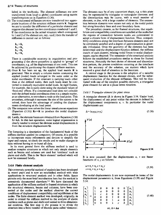
A triangular element ijk is shown in Figure 3.14. Under load,the displacement of any point within the element is defined bythe displacement components M, v. In particular the nodaldisplacements are:

A^fyi^v^vJ (3.38)

It is now assumed that the displacements u, v are linearfunctions of x, y as follows:

M = a, + a2x + a3>> ,3 3^v=a4 + a5x + a6y

The nodal displacements A are now expressed in terms of thedisplacement parameters a, from Equations (3.39) and Figure3.14:

M1I Pl O O O O O ITa1"MJ 1 a O O O O a2

«k 1 c b O O O a3v; ~ O O O 1 O O a4 ^ }

v. O O O 1 a O a5

vk O O O 1 c b a6

or, A = Aa

Figure 3.14

The strains in the element are functions of the derivatives of uand v as follows:

Fe, I Tdu/dx -|€= UJ = \dv/dy (3.41)

[^,J \duldy + dvldx\

«.Po 1 O O O ol a2 (3-42)

= O O O O O 1 ^O O 1 O 1 O a<U- J OC5

« 6 _

i.e.:

C = Ba = BA-1A (3.43)

from Equation (3.40).

It should be noted that the matrix B in Equation (3.42) containsonly constant terms and it follows that the strains are constantwithin the element.

The stress-strain relationships for plane stress in an isotropicmaterial with Poisson's ratio v and Young's modulus E are:

0\ 1 v O £v<j,. = E

(1-v2) v 1 O £v

T,, O O Kl -v) yxy

i.e.:

C=DE=DBA 1A (3.44)Matrix D is the 'elasticity' matrix relating stress and strain. Toobtain the element stiffness we employ the principle of virtualwork and apply arbitrary nodal displacements A producingvirtual strains in the element:

§ = BA 1A (3.45)

The virtual strain energy in the element, from Equation (2.78) ofChapter 2, is:

J1-FcIdK

where V= volume of triangular element = tab/2, / = thicknessSubstituting for 1T and <r from Equations (3.45) and (3.44)respectively, the virtual strain energy is:

Jvo/ [BA-1AfDBA-1AdK

Now since all the matrices contain constant terms only and arethus independent of jc and y, the expression for the virtual strainenergy may be written:

Ar{[A-']rBr DBA' 1K)A

The external work is the product of the virtual displacements Aand the nodal forces S, hence equating external virtual work andinternal virtual strain energy:

A7-S = AM[A-1FB7-DBA-1K)A

The virtual displacements are quite arbitrary and in particularmay be taken to be represented by a unit matrix, thus:

S = {[A ']rBrDBA-'K}A= kA, from Equation (3.30)

Thus:

k = [A 1J7B7DBA 1 K (3.46)

Before the matrix multiplications required in Equation (3.46)can be performed we need to find A~ ' . This is easily determinedas:

" ab 0 0 0 0 0 "- b b O O O O

1 (c~a) - c a O O OA - ' = ^ O Q Q a b O O

O O O -b b OO O O (c-a) - c a _

Hence finally, with | A1 = J(I ~ v) and ^2 = iO + v) we obtain the

stiffness matrix for the plane stress triangular element as shownin equation (3.47) below.

It is neither necessary nor economical to carry out theseoperations by hand; the computation of the element stiffnessand, indeed, the entire computational process is easily pro-grammed for the digital computer.

Computer 'packages' for finite element analysis of structuresare highly developed, very powerful and readily available.Because of the comparatively heavy demands on computerstorage, the use of the packages is generally confined to main-frame computers. A good example of a finite element systemwhich is used very extensively is PAFEC.6 The more importanttopics which should be studied in pursuing finite elementanalysis include: (1) shape (displacement) functions; (2) con-forming and nonconforming elements; (3) isoparametric ele-ments; and (4) automatic mesh generation.

k_ Et2(1-V2)^

b2 + ^(c-a)2

-b2- ̂ c(C- a)

^a(c -a)

-I2b(c-a)

^b(c -a)+vcb

— vab

£2+V2

— k\ac

^cb + vb(c-d)

-A2bc

vab

w— ̂ ab

^ab

O

^b2 + (c-a)2

-^b2-c(c-a)

a(c-a)

Symmetric

V>2 + c2

— ac a2

(3.47)

3.5 Moment distribution

3.5.1 Introduction

Although the stiffness method, described in the previous sectionhas the merit of simplicity, the solution of the equilibriumequations (3.31) is generally a matter for the digital computersince only for the simplest structures can a hand solution becontemplated. An alternative procedure which is eminentlysuitable for hand computation is the method of moment distri-bution which is essentially an iterative solution of the equationsof equilibrium.

As in the general stiffness method, we first imagine all thedegrees of freedom, joint rotations and joint translations, to beconstrained. We ignore axial effects in members and considerflexure only. The constraints are imagined to be clamps appliedto the joints to prevent rotation and translation. The forcesrequired to effect the constraints are applied artificially and inthe moment distribution processes these clamping forces aresystematically released so as to allow the structure to achieve anequilibrium state. It is important to note that in the method asgenerally applied, the rotational joint restraints are relaxed byone process and the translational restraints by another. Finallythe principle of superposition is used to combine the separateresults.

It is necessary to assemble certain standard results before wecan consider the actual process.

3.5.2 Distribution factors, carry-over factors andfixed-end moments

For the time being we confine our attention to prismaticmembers. The treatment of nonuniform section members will betouched on later.

Standard member stiffnesses are required and these are illus-trated in Figure 3.15. The member end forces are those requiredto produce the deflected forms shown. Diagrams (a) and (b)relate to rotation without translation (sway), and diagrams (c)and (d) relate to sway without rotation. The results in diagrams(a) and (c) may be deduced from the stiffness matrix in Equation(3.30). The other results may be obtained easily from elementarybeam theory, e.g. in Figure 3.15(b), taking the origin of x at theleft-hand end and y positive downwards:

Ely = ™ ^+ (BIO- M L^ x + C2

= 0 for jc=0; hence C2 = O

n f i u ., *EI°= O for x = /; hence, M=—-.—

When loads are applied to members which are constrained atthe joints, fixed-end moments are required to prevent the endrotations. This is another standard type of result which isrequired in the moment distribution method. Table 3.5 listsfixed-end moments for a selection of loading cases on uniformsection beams. Again, these results may be obtained fromelementary beam theory. It should be noted that the signconvention is that a moment is positive if tending to produceclockwise rotation of the end of the member at which it acts.This convention is different to, and should not be confused with,the sign convention for constructing bending moment diagramswhich must be based on the curvature produced in the member.

As an illustration of the basic process, consider the structureABC shown in Figure 3.11. This structure was analysed by thestiffness method previously. Joint B is considered to be clampedand thus a system of fixed-end moments is set up in member AB.The end moments in the members are shown in line 1 of Table3.6. The constraining moment at joint B is seen to be Wl J%clockwise and we imagine this moment to be removed by theapplication of a moment - Wl1 /8. The subsequent rotation ofjoint B, anticlockwise through angle 0, will develop moments inboth members. Referring to Figure 3.15 the moments inducedwill be:

_ 4EIO m _ 2EIOMBA- ~—,—» ^AB- ~—J—11 'i

M _ *EW. M _ i™MB C— — —.—, MCB — ——.—12 12

For equilibrium of joint B, the applied moment - W/,/8 mustequal the sum of the moments absorbed by the two membersmeeting at the joint:

-2--^--(H)and it is seen that the moment is 'distributed' to the members inproportion to their /// values.

Thus:

_-Wl, Ul, _~Wl,( I2 \MBA 8 (///,+///,) 8 U + /J

and:

_-»7, ///, _-WlJ I1 \MK 8 (///, + ///,) 8 U + /2/

The moments induced at A and C are from Figure 3.15, one-halfof those induced at B and the factor of one-half is termed thecarry over factor. This set of moments is shown in line 2 of Table3.6.

Joint B is now 'in balance' and since it was the only jointwhich was clamped we have reached an equilibrium state and nofurther distribution of moments is required. The final set of

Figure 3.15

EId2y/dx2 = —j-, where M is the moment, to be determined, at

the right-hand end,

Eldy/dx = ̂ - y+C,

= EI8 for x = l; hence C, = EIO-M^

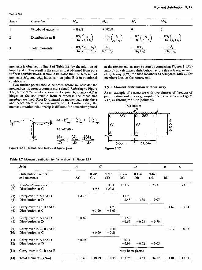
Table 3.6

Stage Operation MAB

1 Fixed-end moments - Wl1 /8

2 Distribution at B -J¥L (-^~\16 U + /J

3 Total moments _ K7,/2/, + 3/2\16 v / ,+ / 2 ;

moments is obtained in line 3 of Table 3.6, by the addition oflines 1 and 2. This result is the same as that obtained from purestiffness considerations. It should be noted that the zero sum ofmoments MBA and MBC indicates that joint B is in rotationalequilibrium.

Two further points should be noted before we consider themoment distribution process in more detail. Referring to Figure3.16, of the three members connected at joint A, member AD ishinged at the end remote from A whereas the other twomembers are fixed. Since D is hinged no moment can exist thereand hence there is no carry-over to D. Furthermore, themoment-rotation relationship is different for a member pinned

MBA MBC A/CB

+ f*7,/8 O O

_wi±(_k\ _MI(JL_\ -™i(Ji_\8 V/. + /2/ 8 U + /2/ 16 V/ ,+ /2/

Wl1, IVP, WP,8(/, + /2) 8(/, + /2) 16(/, + /2)

at the remote end, as may be seen by comparing Figures 3.15(a)and (b). In calculating distribution factors this is taken accountof by taking J(//0 for sucn members as compared with /// formembers fixed at the remote end.

3.5.3 Moment distribution without sway

As an example of a structure with two degrees of freedom ofjoint rotation and no sway, consider the frame shown in Figure3.17, EI (beams) = 3 x EI (columns).

Figure 3.16 Distribution factors at typical joint Figure 3.17

Table 3.7 Moment distribution for frame shown in Figure 3.17

Joint

Distribution factorsend moments

(1) Fixed-end moments(2) Distribution at C

(3) Carry-over to A and D(4) Distribution at D

(5) Carry-over to C, B and E(6) Distribution at C

(7) Carry-over to A and D(8) Distribution at D

(9) Carry-over to C, B and E(10) Distribution at C

(11) Carry-over to A and D(12) Distribution at D

(13) Carry-over to C, B and E

(14) Total moments (kNm)

A

AC

+ 4.75

+ 0.60

+ 0.05

+ 5.40

C

0.285CA

+ 9.5

+ 1.20

+ 0.09

+ 10.79

0.715CD

-33.3+ 23.8

-4.23+ 3.03

-0.30+ 0.21

- 10.79

D

0.386 0.154DC DB

+ 33.3

+ 11.9-8.45 -3.38

+ 1.52-0.59 -0.23

+ 0.11-0.04 -0.02

May be neglected

+ 37.75 -3.63

0.460DE

-23.3

- 10.07

-0.70

-0.05

-34.12

B

BD

-1.69

-0.12

-1.81

E

ED

+ 23.3

-5.04

-0.35

+ 17.91

The fixed-end moments are, (w/2/12),

MFCD= -30x2^!; MFDC= + 30 x ̂ = 33.3 kNm

^FDE= -30x^ MFED= +30x^=23.3 kNm

and the distribution factors are:

atC CD-CA- 3/3'65 • I/3-°5

' ' (1/3.05) + (3/3.65)' (1/3.05) + (3/3.65)= 0.715:0.285

at D, DC:DB:DE =

3/3.65 1/3.05(3/3.65) + (1/3.05) + (3/3.05): (3/3.65) + (1/3.05) + (3/3.05):

3/3.05(3/3.65) + (1/3.05) + (3/3.05)

= 0.386:0.154:0.460

The moment distribution is carried out in Table 3.7. It should benoted that after each distribution at a joint the distributedmoments are underlined to indicate that the joint is balanced atthat stage. At step 4, the out-of-balance moment to be distri-buted at D is + 33.3+11.9-23.3= +21.9; hence the distributedmoments should total -21.9.

3.5.4 Moment distribution with sway

This process will be illustrated with reference to Example 3.3(page 3/9), for which the structure is shown in Figure 3.9. Wefirst ignore any horizontal movement (sway) of the joints B andC and carry out a moment distribution.

The fixed-end moments are w/2/12 = ±40kNm; and the dis-tribution factors are:

BA:BC = i:f

CB: CD = f: i (noting J/// for CD)

The result of this (no sway) moment distribution is given in line3 of Table 3.8. We now consider the horizontal equilibrium ofthe beam BC, Figure 3.18(a), and find that a force F1 is requiredto maintain equilibrium. F1 may be calculated by evaluating thehorizontal shear forces at the tops of the columns as follows:

F, = 120 + (20±M-20=I2(,8kN

This force cannot exist in practice and what happens is that thebeam BC deflects to the right and a new set of bending momentsis set up with the effect that the out-of-balance horizontal forceF1 is removed. We consider the effect of this sway separately.Referring to Figure 3.18(b), a movement to the right of A,without joint rotation, requires column moments as shown.From Figure 3.15(c) and (d), these column moments are,

^FBA = ^FAB= ~6 ( -JT J AAB

Figure 3.18

MFCD= - 3 (|Q ACD (note MFDC = O)

We cannot evaluate these moments unless A is known but wecould proceed with an arbitrary value of A, and carry out adistribution to produce rotational equilibrium of the joints Band C. In fact, it is seen that any arbitrary values of momentscan be used providing these are in the correct proportionsbetween the two columns. The ratio in this example is:

»=»-(*) 40')\* / A B >' 'CD

If we adopt

^FBA = A/FAB =-90

and

MFCD =-80

the moments are in the correct proportion. A second momentdistribution is now carried out, using these values of fixed-endmoments, and the result is shown in line 1 of Table 3.8. This setof moments is consistent with an applied horizontal force F2,Figure 3.18(c), and:

^^±Z5+^56.3kN

Table 3.8

Joint A B C

End moments AB BA BC CB CD

(1) Arbitrary sway -78 -66 +66 +61 -61(2) Corrected [(1) x A] -167 -141 +141 +131 -131(3) No sway moments +10 +20 - 20 +20 - 20(4) Final moments

[(2) + (3)] -157 -121 +121 +151 -151

Now F2 has to be scaled to equal F1 and the scaling factor is F1/F2 = A= 120.8/56.3 = 2.14.

The corrected moments are given in line 2 of Table 3.8 and thefinal moments are in line 4 obtained by adding lines 2 and 3.

3.5.5 Additional topics in moment distribution

Space has permitted only a brief introduction to the method ofmoment distribution. Additional topics which should be studiedby reference to the standard texts,3-4 are as follows:

(1) Frames with multiple degrees of freedom for sway. Theseare handled by carrying out an arbitrary sway distribution

for each sway in turn. Equilibrium conditions are then usedto relate the out-of-balance forces and obtain the correctionfactors for each sway mode.

(2) Treatment of symmetry. In cases of symmetry the momentdistribution process can be considerably shortened. Twocases arise and should be studied, systems in which it isknown that the final set of moments is symmetrical andsystems in which the final moments form an anti-symmetri-cal system.

(3) Nonprismatic members. If the flexural rigidity (EI) of amember varies within its length, then the effect is to changethe values of end stiffnesses, carry-over factor and fixed endmoments. A suitable general method for handling thissituation is to evaluate end flexibilities by the use of Simp-son's rule and then convert the flexibilities into stiffnesses.

3.6 Influence lines

3.6.1 Introduction and definitions

It is frequently necessary to consider loads which may occupyvariable positions on a structure. For example, in bridge designit is important to determine the maximum effects due to thepassage of a specified train or system of loads. In other cases thetotal load on a structure may be comprised of different loadswhich may be applied in various combinations and this again isa problem of variability of load or load position. The effect ofvarying a load position may be studied with the help of influencelines.

An influence line shows the variation of some resultant actionor effect such as bending moment, shear force, deflection, etc. ata particular point as a unit load traverses the structure. It isimportant to observe that the effect considered is at a fixedposition, e.g. bending moment at C, and that the independentvariable in the influence line diagram is the load position. Thefollowing is a summary of influence line theory. For a moredetailed treatment the reader should consult Jenkins.1

3.6.2 Influence lines for beams

Consider the simply-supported beam AB, Figure 3.19, carryinga single unit load occupying a variable position distant y fromA. We require to obtain influence lines for bending moment andshear force at a fixed point X distant a from A and b from B.

If the unit load lies between X and B:

MK = R^a=\^j^-a (3.48)

If the unit load acts between A and X:

MK = RB'b = l-y/l'b (3.49)

Equations (3.48) and (3.49) are linear in y and when plotted inthe regions to Which they relate, form a triangle as shown inFigure 3.19(b). We note that, in both cases, substitution of y = agives Mx = 1 -ab/l. Thus the influence line for Mx is a triangle witha peak value ab/l at the section X.

Turning now to the influence line for shearing force at X. Forunit load between X and B:

Sx = *A = ̂ (3.50)

(and now we have implied a sign convention for shear force

Figure 3.19 Influence lines and related diagrams for simplysupported beams

namely that Sx is positive if the resultant force to the left of thesection is upwards).

Where ^ = a, SK = b/l

For unit load between A and X:

S11=-R9=-y/l (3.51)

when y = a, Sx = — a/7

We note that Equations (3.50) and (3.51) give different values ofSx for y = a and moreover the signs are opposite. This meansthat the shear force influence line contains a discontinuity at Xas shown in Figure 3.19(c).

In using influence lines with a given system of loads andhaving determined the locations of the loads on the span, thetotal effect is evaluated as:

£(WX ordinate), for concentrated loads (3.52)

and:

(whdx= w (area under influence line) (3.53)

for distributed loads (Figure 3.19(d).The maximum effect produced at a given position is of

interest in the design process. In the case of concentrated loads,from Equation (3.52), this is obtained when:

£( W x ordinate) is a maximum

The process of locating the loads to produce the maximum valueis best done by trial and error. It follows from the straight-linenature of a bending moment diagram due to concentrated loads,that the maximum bending moment at a section will be obtainedwhen one of the loads acts at the section. This may be illustratedby reference to the two-load system shown at (e) in Figure 3.19.The shape of the bending moment diagram is as shown at (O andat (g) is drawn a diagram which shows the maximum value ofbending moment at any section in the beam. This is themaximum bending moment envelope Afmax which is seen to consistof two intersecting parabolic curves Afyl and Afy2.

The curve Afyl represents the maximum bending moment atall sections in the beam when this is obtained with load IV}

placed at the section. The curve Afy2 represents the maximumbending moment at all sections in the beam when this isobtained with load IV2 at the section. It is seen that W1 should beplaced at the section towards the left-hand end of the beam, andW2 at the section towards the right-hand end of the beam.

The expressions for Afy, and Afy2 are as follows:

M^ = (W,+W^i(I-y,-a)

(3.54)

M^ = (W1+W$-f&(yi-b)

In the case of a distributed load which has a length greater thanthe span, then for an influence line of type (b) in Figure 3.19, thewhole span would be loaded, whereas for an influence line oftype (c) one would place the left-hand end of the load at X thusavoiding the introduction of a negative effect on the maximumpositive value. For a short distributed load, as at (h), formaximum effect at y, the load must be placed so that the shadedarea in (j) is a maximum.

The rule for this is:

y 11= ale (3.55)

3.6.3 Influence lines for plane trusses

In the analysis of plane trusses, the influence line is useful inrepresenting the variations in forces in members of the truss.

Figure 3.20(a) shows a Warren girder AB of span 20m. Forthe unit load acting at any of the lower chord joints, the force inmember 1 is:

p_^A

^'-273

The peak value occurs when the unit load is at C, and thus:

P =Ax 4xl=J-^1""" V3 5 l 5V3

The influence line for P1 is shown at (b).For member 2, if the unit load lies between A and E, we take:

Figure 3.20 Influence lines for plane truss

n-12*,2 2V3

or, if the unit load lies between E and B we take:

p _ 8 * A

^2~275

The result is a triangle with peak value 12/Sx/3 at E, as shown indiagram (c).

It should be noted that both the P1 and P2 influence linesindicate compression for all positions of the unit load.

For members 3 and 4 it is useful to note that these memberscarry the vertical shear force in the panel CE, and we proceed bydrawing the influence line for VCE as at (d).

Considering now the force in member 3 and the section XX indiagram (a), it is clear that the relationship is:

p- ^CE3 sin 60°

and that P3 is tensile when VCE is positive and compressive whenVCE is negative.

3.6.4 Influence lines for statically indeterminatestructures

The use of influence lines in representing the effects of variable-position loads in statically determinate beams and trusses hasbeen outlined. The concept is, of course, of general application.When dealing with statically indeterminate structures it isconvenient to introduce some additional theorems to assist theanalysis. It is possible to relate influence line shapes to deflectedshapes of structures under particular forms of applied force.This involves an application of Mueller-Breslau's principle,which we shall look at in this section. The application of thisprinciple can take the form of a model analysis, to which asimple form or model of the structure is made and particulardistortions of the model produce scaled versions of influencelines.

Compression

Figure 3.21

The first bracket in Equation (3.56) contains the work doneduring the application of W and the second bracket the workdone (by both M and W) during the application of M.

In a similar way, if the order is reversed, the work done is:

(iM/22) + (i^/u + M/2l) (3.57)

From Equations (3.56) and (3.57) it is evident that:

JVf12 = Mf21 (3.58)

If the applied actions are taken to have unit values, thenEquation (3.58) simplifies to:

/I2=/2, (3.59)

Equation (3.59) is a statement of Maxwell's reciprocal theorem.A more general theorem, of which Maxwell's is a special case, isdue to Betti. This latter theorem states that if a system of forcesP1 produces displacements p} at corresponding positions andanother set of forces Q^ at similar positions to P-, producesdisplacements ^1, then:

^1+^202+ . . - +^=e./>, + C2/>2+ ." +QnPn (3-60)

3.6.6 Mueller-Breslau's principle

This principle is the basis of the indirect method of modelanalysis. It is developed from Maxwell's theorem as follows.Consider the two-span continuous beam shown in Figure3.22(a). On removal of the support at C and the application of aunit load at C, a deflected shape, shown dotted in Figure

3.22(b), is obtained. If a unit load now occupies any arbitraryposition D, as at (c), then from Maxwell's theorem the deflec-tion at C will be S0. In other words, the deflected form (b) is theinfluence line for deflection of C.

Now the force at C to move C through Sc = 1Hence, the force at C to move C through ^= 1 x SD/SC.If a unit load acts at D, producing a deflection SD at C, then

the upwards force needed to restore C to the level of AB is1 x 6D/SC. Hence, the reaction at C for unit load at D is 1 x SJS0.Since D is an arbitrary point in the beam then it is seen that thedeflected shape due to unit load at C, Figure 3.22(b), is to somescale, the influence line for Rc. The scale of the influence line isdetermined from the knowledge that the actual ordinate at Cshould equal unity. Hence, the ordinates should all be dividedby<5c.

This result leads to Mueller-Breslau's principle which may bestated as follows:

'The ordinates of the influence line for a redundant force areequal to those of the deflection curve when a unit loadreplaces the redundancy, the scale being chosen so that thedeflection at the point of application of the redundancyrepresents unity.'

With the enormous increase in computing power now avail-able there is little need to use models in this way and it isgenerally more economical to produce influence lines by com-puter. It should be noted that it is always possible to constructinfluence lines by repeated analysis of the structure under a unitapplied load, changing the load position for each analysis andthus producing a succession of ordinates to the influence linesought. This latter approach will be illustrated in section 3.6.8.

We now look at two important theorems concerned withinfluence lines.

3.6.5 Maxwell's reciprocal theorem

Consider the propped cantilever shown in Figure 3.21 to besubjected to a load Wat A, producing displacements/, and/21as shown at (a), and then separately to be subjected to a momentM at B producing displacements/J2 and/22 as at (b). Assuming alinear load-displacement relationship we may use the principleof superposition and obtain the combined effects of W and M byadding (a) and (b). Clearly it will be immaterial in which orderthe forces are applied. Applying W first and then M, the workdone by the loads will be:

(Wn) +(P^22+tf/12) (3.56)

Figure 3.22

3.6.7 Application to model analysis

Consider the fixed arch shown in Figure 3.23(a). The arch hasthree redundancies which may be taken conveniently as //A, VKand MA. We make a simple model of the arch to a chosen linearscale and pin this to a drawing board. End B is fixed in positionand direction and the undistorted centreline is transferred to thedrawing paper. We then impose a purely vertical displacementAv at A and transfer the distorted centreline to the drawingpaper. The distortion produced will require force actions at A,V\ H' and M'. Let the displacement of a typical load point beAw. Applying Equation (3.60) to the two systems of forces:

KA(AV) + //A_(0) + MA(0) + Jf(AJ = F'(0) + If(Q) + Kf(O) + 0(S)

Hence:

FA+JTA^O

and if W=I:

Figure 3.23

FA = -̂ (3.61)

Similarly, we impose a purely horizontal displacement AH andobtain:

"* = -^ (3-62>

then a pure rotation 9 and obtain:

^A=--/ (3.63)

In Equations (3.62) and (3.63) the displacements A^, and A^represent the arch displacements due to the imposed horizontaland rotational displacements respectively. In each case thedeflected shape, suitably scaled, gives the influence line for thecorresponding redundancy.

3.6.7.1 Sign convention

The negative sign in Equations (3.61) to (3.63) leads to thefollowing convention for signs. On the assumption that areaction is positive if in the direction of the imposed displace-ment, then a load W will give a positive value of the reaction ifthe influence line ordinate at the point of application of the loadis opposite to the direction of the load. This is evident in Figure3.23(b) where the upward deflection A1,, being opposed to thedirection of the load W, is consistent with a positive (upwards)direction for KA.

Unit Load Positions

3.67.2 Scale of the model

It should be noted that when using relationships (3.61) and(3.62) the ratios AW/AV and A'W/AW are dimensionless and thus thelinear scale of the model does not affect the influence lineordinates. On the other hand, when using Equation (3.63) inobtaining an influence line for bending moment, AJO has thedimensions of length and thus the model displacements must bemultiplied by the linear scale factor.

In performing the model analysis, quite large displacementscan be used providing the linear relation between load anddisplacement is maintained. Hence, the indirect method issometimes called the 'large displacement' method.

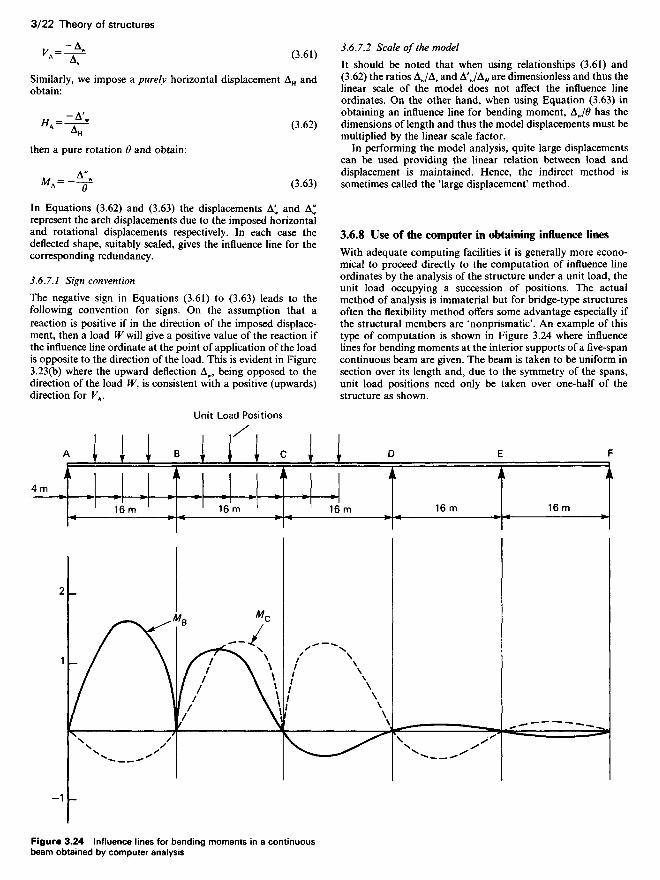
3.6.8 Use of the computer in obtaining influence lines

With adequate computing facilities it is generally more econo-mical to proceed directly to the computation of influence lineordinates by the analysis of the structure under a unit load, theunit load occupying a succession of positions. The actualmethod of analysis is immaterial but for bridge-type structuresoften the flexibility method offers some advantage especially ifthe structural members are 'nonprismatic'. An example of thistype of computation is shown in Figure 3.24 where influencelines for bending moments at the interior supports of a five-spancontinuous beam are given. The beam is taken to be uniform insection over its length and, due to the symmetry of the spans,unit load positions need only be taken over one-half of thestructure as shown.

Figure 3.24 Influence lines for bending moments in a continuousbeam obtained by computer analysis

3.7 Structural dynamics

3.7.1 Introduction and definitions

Structural vibrations result from the application of dynamicloads, i.e. loads which vary with time. Loads applied to struc-tures are often time-dependent although in most cases the rateof change of load is slow enough to be neglected and the loadsmay be regarded as static. Certain types of structure may besusceptible to dynamic effects; these include structures designedto carry moving loads, e.g. bridges and crane girders, andstructures required to support machinery. One of the mostsevere and destructive sources of dynamic disturbance of struc-tures is, of course, the earthquake.

The dynamic behaviour of structures is generally described interms of the displacement-time characteristics of the structure,such characteristics being the subject of vibration analysis.Before considering methods of analysis it is helpful to definecertain terms used in dynamics.

(1) Amplitude is the maximum displacement from the meanposition.

(2) Period is the time for one complete cycle of vibration.(3) Frequency is the number of vibrations in unit time.(4) Forced vibration is the vibration caused by a time-dependent

disturbing force.(5) Free vibrations are vibrations after the force causing the

motion has been removed.(6) Damping. In structural vibrations, damping is due to: (a)

internal molecular friction; (b) loss of energy associatedwith friction due to slip in joints; and (c) resistance tomotion provided by air or other fluid (drag). The type ofdamping usually assumed to predominate in structuralvibrations is termed viscous damping in which the forceresisting motion is proportional to the velocity. Viscousdamping adequately represents the resistance to motion ofthe air surrounding a body moving at low speed and also theinternal molecular friction.

(7) Degrees of freedom. This is the number of independentdisplacements or coordinates necessary to completely definethe deformed state of the structure at any instant in time.When a single coordinate is sufficient to define the positionof any section of the structure, the structure has a singledegree of freedom. A continuous structure with a distributedmass, such as a beam, has an infinite number of degrees offreedom. In structural dynamics it is generally satisfactoryto transform a structure with an infinite number of degreesof freedom into one with a finite number of freedoms. Thisis done by adopting a lumped mass representation of thestructure, as in Figure 3.25. The total mass of the structure isconsidered to be lumped at specified points in the structureand the motion is described in terms of the displacements ofthe lumped masses. The accuracy of the analysis can beimproved by increasing the number of lumped masses. Inmost cases sufficiently accurate results can be obtained witha comparatively small number of masses.

Distributed moss beam Lumped mass beam

Figure 3.25

3.7.2 Single degree of freedom vibrations

The portal frame shown in Figure 3.26 is an example of astructure with a single degree of freedom providing certainassumptions are made. If it is assumed that the entire mass of

Figure 3.26

the structure (M) is located in the girder and that the girder hasan infinitely large flexural rigidity and further, that the columnshave infinitely large extensional rigidities, then the displacementof the mass M resulting from the application of an exciting force/*(/), is defined by the transverse displacement y. The girdermoves in a purely horizontal direction restrained only by theflexure of the columns.

From Newton's second law of motion:

Force = mass x acceleration

i.e.:

£P=My (3.64)

Now from Figure 3.26(b), the force resisting motion is:

a-, (^S)

-«f (3.65,

Thus Equation (3.64) becomes:

P(t) -24 ̂ = My

or:

My + IA^-W (366)

If the effect of damping is included then the equation of motion,Equation (3.66) is modified by the inclusion of a term cy where cis a constant. It should be noted that since the effect of dampingis to resist the motion, then the term cy is added to the left-handside of Equation (3.66). Thus:

My + cy + 2A~£ = P(t) (3.67)

Equation (3.67) may be generalized for any single degree offreedom structure by observing that the stiffness of the struc-ture, i.e. force required for unit displacement horizontally, isgiven by:

*-24^*'** V (3.68)

Combining Equations (3.67) and (3.68) we obtain the generalsingle degree of freedom equation of motion:

My + <$ + ky = P(t) (3.69)

If in Equation (3.69) P(t) = O, we have a state of free vibration ofthe structure. The governing equation becomes:

My + cy + ky = 0 (3.70)

The situation envisaged by Equation (3.70) would arise if thebeam were given a horizontal displacement and then released.The resulting vibrations would depend on the amount ofdamping present, measured by the coefficient c.

The solution of Equation (3.70) is:

y = A,e* + &fh? (3.71)

where A1 and A2 are the constants of integration, to be evaluatedfrom initial conditions, and A1 and A2 are the roots of theauxiliary equation:

AfA2 -I- cA + k = O (3.72)

or, substituting:

P2 = h/M \

and I (3.73)2n = c/M I

Equation (3.72) becomes:

A2 + 2wA+/72 = 0 (3.74)

Hence:

A=-«±V(«2-/>2) (3.75)

Four cases arise:

Case 3.1 p2<n2

Here (rf—p2) is always positive and <n2 and thus A1 and A2 arereal and negative.

Equation (3.71) takes the form:

y = e'"t(A^"2~^t^A2e-^2-^') (3.76)

The relationship between y and / of Equation (3.76) is shown inFigure 3.27(a) and it is seen that the displacement y graduallyreturns to zero, no vibrations taking place.

Now, since n2>p2, then:

^!_>A4M2 M

or

02J(Mk) (3.77)

A structure exhibiting these characteristics is said to be over-damped.

Case 3.2 p2 = n2

From Equation (3.75), A-AJ (twice)and hence,

y = e-«(Ai + A2t) (3.78)

Figure 3.27

This is termed critical damping and the critical dampingcoefficient cc is the value of the damping coefficient at theboundary between vibratory and nonvibratory motion. Thecritical damping coefficient is a useful measure of the dampingcapacity of a structure. The damping coefficient of a structure isusually expressed as a percentage of the critical dampingcoefficient.

Case 3.3 p2>n2

Here c < cc and the structure is underdamped.From Equation (3.75), A= -n±ij(p2-n2)Hence:

y = £>-%VV("2~"2)' + A2e-^2-n2)t)

or, putting:

(P2~n2) = q2

y = e-nt(A]eit" + A2e-Ui')

or

y = e ~ "'(A cos qt + B sin qt) (3.80)

A typical displacement-time relationship for this condition isshown in Figure 3.27(b).

An alternative form for Equation (3.80) is:

y = Ce ntsin(qt + fi) (3.81)

where C and /? are new arbitrary constants

~i • j rr, 2n 2nThe period T= — = —T71—( , .,.F q pj{l-(n/p)2}

The period is constant but the amplitude decreases with time.The decay of amplitude is such that the ratio of amplitudes atintervals equal to the period is constant, i.e.:

y(t) — gnT

y«+T>and log e"T=nT=6

Again, no vibrations result and Equation (3.78) has the formshown in Figure 3.27(a).

From Equation (3.73) the value of c for this condition is givenby:

cc = 2J(Mk) (3.79)

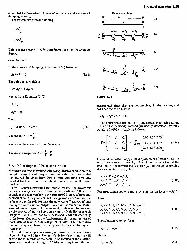
S is called the logarithmic decrement, and is a useful measure ofdamping capacity.

The percentage critical damping

= 10(£Cc

-'«£

This is of the order of 4% for steel frames and 7% for concreteframes.

Case 3.4 c = 0

In the absence of damping, Equation (3.70) becomes:

My + ky = 0 (3.82)

The solution of which is:

y = A]e*\' + A2e^t

where, from Equation (3.72):

A1 = ip

I2=-ip

Thus:

y = A sinpt + Bcospt (3.83)

The period is, T=-

where p is the natural circular frequency

The natural frequency is/= ~=y-

3.7.3 Multi-degree of freedom vibrations

Vibration analysis of systems with many degrees of freedom is acomplex subject and only a brief indication of one usefulmethod will be given here. For a more comprehensive anddetailed treatment, the reader should consult one of the stan-dard texts.7

For a system represented by lumped masses, the governingequations emerge as a set of simultaneous ordinary differentialequations equal in number to the number of degrees of freedom.Mathematically the problem is of the eigenvalue or characteristicvalue type and the solutions are the eigenvalues (frequencies) andthe eigenvectors (modal shapes). We shall consider the evalu-ation of mode shapes and fundamental, undamped, frequenciesby the process of matrix iteration using the flexibility approach(see page 3/6). The method to be described, leads automaticallyto the lowest frequency, the fundamental, this being the one ofmost interest from a practical point of view. The alternativemethod using a stiffness matrix approach leads to the highestfrequency.

Consider the simply-supported, uniform cross-section beamshown in Figure 3.28(a). The mass/unit length is w and we willregard the total mass of the beam to be lumped at the quarter-span points as shown in Figure 3.28(b), We may ignore the end

Figure 3.28

masses w//8 since they are not involved in the motion, andconsider the three masses

Af, = Af2 = Af3 = H>//4.

The appropriate flexibilities,/^ are shown at (c), (d) and (e).Using the flexibility method previously described, we may

obtain a flexibility matrix as follows:

~/, fi2 /i3~l |~3.00 3.67 2.33 ~

F= /21 /22 /M =25M7 3'67 5'33 3'67 (3'84)

/3, /32 /33J L2'33 3'67 3-°°_

It should be noted that/j is the displacement of mass Af1 due tounit force acting at mass M-. Thus, if the forces acting at thepositions of the lumped masses are F12>3 and the correspondingdisplacements are 7,23, then:

>>,=/;, F1 -KTi2F2 +f}3F3]J2-/2,*1,+/22*2+/23*3 (3-85)^3=/;.*1.+/32*2+/33*3 J

For free, undamped vibrations, F1 is an inertia force= — Mty{.

Thus:

>>, +/,W, +/,2^2 +/,3^3 = O ]

^2 +/2 W, +/22^2*2 +/23^3* = O (3.86)

y, +/3,^, +/32^2 +/33^F3 = O j

The solutions take the form:

y, = S1 cos (pt + a) (3.87)

Hence:

y~~P2yt (3-88)

Moss w /unit length

Thus, Equations (3.86) become:

<5, -/,,M./72 <5, -/,2 ̂ 2^2-/,3 **3/>2 ^3 = 0

<*2 -/2,M,/>2 <5, -/22 ̂ 2^2 ~/23 ̂ 3 /^3 = 0 (3.89)

<53-/3,^,/>2 <*, -/32 M2^2-/33 M3/ <53 = O)

or:

A=/72FMA (3.90)

where:

"̂ 1"] FM, o o n

A= S2 • M= O M2 O<53 I O O M3

The unknowns in Equation (3.90) are the displacement ampli-tudes S{ and the frequency p\ p has as many values as there areequations in the system, and for every value of p (eigenvalue)there corresponds a set of y (eigenvector).

We adopt an iterative procedure for the solution of Equation(3.90) and first of all rewrite the equations in the form:

FMA=^A (3.91)

We start with an assumed vector A0, thus:

FMA0=^A0

Putting FMA0 = A1

A1 ̂ 2 A0 giving p2^

We cannot form A0/A, since each A is a column matrix, so wetake the ratio of corresponding elements in A0 and A, and formthe ratio 6Jd1. It is best to use the numerically greatest 6 for thispurpose.

Continuing the process:

FMA1^2-A1 giving p2 = 6} /S2

= A2

and again:

FMA2=^A2

= A3 giving P2^=S2IS3

It can be shown that this iterative process converges to thelargest value of l/p2 and hence yields the lowest (fundamentalmode) frequency.

Applying the iterative scheme to the beam of Figure 3.28, andassuming:

*••[?]

then, A1 = FMA0

/3 [3.00 3.67 2.33~j Pw//4 O O ~|where FM = -~- 3.67 5.33 3.67 O w//4 O

Z^hI J^2 33 3 67 3 QOJ Jj) 0 w//4j

/4 |~3.00 3.67 2.33~= ™ 3.67 5.33 3.67

W24L1 j^2 33 3 6? 3 0()̂

TH A "'4 [££l «-«™'["!-£lTh- A'-l^[!«$J-T^[j;£]

„ , 6a 2 x 1024£/Hence: P^= 12 6?x , 42,,/4

= 114^w/4

A second iteration gives:

,. T3.00 3.67 2.33"! ,.,, .. ~i.00~A =FMA = Wl 3.67 5.33 3.67 12'67vv/ 1.42A> FMA' 1024*7 [233 367 3.Q0J 1024£/ [L00_

/ wi> v T10-54]

= 12.67177̂ =-. 14.91Vio24£/y ^1054J

Hence:

2_^_12.67xl .42w/ 4y 1

P2 S2 IQ24EI X 12.67(M'/4/1024£/)2x 14.91

= 975^w/4

This result is very close to that produced by an exact method,i.e. 97.41£//w/4.

3.8 Plastic analysis

3.8.1 Introduction

The plastic design of structures is based on the concept of a loadfactor (N), where

Collapse load _ Wc 'Working load ~W~W (3.92)

A structure is considered to be on the point of collapse whenfinite deformation of at least part of the structure can occurwithout change in the loads. The simple plastic theory is basedon an idealized stress-strain relationship for structural steel asshown in Figure 3.29. A linear, elastic, relationship holds up to astress Gy, the yield stress, and at this value of stress the material isconsidered to be in a state of perfect plasticity, capable ofinfinite strain, represented by the horizontal line AB continuedindefinitely to the right. For comparison the dotted line showsthe true relationship.

The term 'plastic analysis' is generally related to steel struc-tures for which the relationship indicated in Figure 3.29 is agood approximation. The equivalent approach when dealingwith concrete structures is generally termed 'ultimate loadanalysis' and requires considerable modification to the methoddescribed here.

The stress-strain relationship of Figure 3.29 will now beapplied to a simple, rectangular section, beam subjected to anapplied bending moment M (Figure 3.30).

Under purely elastic conditions, line OA of Figure 3.29, thestress distribution over the cross-section of the beam will be asshown in Figure 3.30(b) and the limiting condition for elasticbehaviour will be reached when the maximum stress reaches thevalue <7y. As the applied bending moment is further increased,material within the depth of the section will be subjected to theyield stress ay and a condition represented by Figure 3.30(c) willexist in which part of the cross-section is plastic and part plastic.On further increase of the applied bending moment ultimatelycondition (d) will be reached in which the entire cross-section isplastic. It will not be possible to increase the applied bendingmoment further and any attempt to do so will result in increasedcurvature, the beam behaving as if hinged at the plastic section.Hence, the use of the term plastic hinge for a beam section whichhas become fully plastic.

Figure 3.30

The moment of resistance of the fully plastic section is, fromFigure 3.30(d):

*, _ L<* d_bd2vM*-b2a>2 4^

= Ze<7w (3.93)

where Zp = plastic section modulus

In contrast, the moment of resistance at working stress crw is,from Figure 3.30(b):

*, -L <J°*2 j-bd2

M»-b2^3d—6*» (3.94)

= Ze<rw

where Ze = elastic section modulus

The ratio Zp/Ze is the shape factor of the cross-section. Thus theshape factor for a rectangular cross-section is 1.5.

The shape factor for an !-section, depth d and flange width b,is given approximately by:

/l+*/2\\l+x/3j

where x = ^T-T and /w and tf are the web and flange thicknesses

respectively

Values of plastic section moduli for rolled universal sections aregiven in steel section tables.

3.8.2 Theorems and principles

The definition of collapse, which follows from the assumed basicstress-strain relationship of Figure 3.29, has already been given.If the structural analysis is considered to be the problem ofobtaining a correct bending moment distribution at collapse,then such a bending moment distribution must satisfy thefollowing three conditions:

(1) Equilibrium condition: the reactions and applied loads mustbe in equilibrium.

(2) Mechanism condition: the structure, or part of it, mustdevelop sufficient plastic hinges to transform it into amechanism.

(3) Yield condition: at no point in the structure can the bendingmoment exceed the full plastic moment of resistance.

In elastic analysis of structures where several loads are acting,e.g. dead load, superimposed load and wind load, it is permiss-ible to use the principle of superposition and obtain a solutionbased on the addition of separate analyses for the differentloads. In plastic theory the principle of superposition is notapplicable and it must be assumed that all the loads bear aconstant ratio to one another. This type of loading is called'proportional loading'. In cases where this assumption cannotbe made, a separate plastic analysis must be carried out for eachload system considered.

For cases of proportional loading, the uniqueness theoremstates that the collapse load factor Nc is uniquely determined if abending moment distribution can be found which satisfies thethree collapse conditions stated.

The collapse load factor Nc may be approached indirectly byadopting a procedure which satisfies two of the conditions butnot necessarily the third. There are two approaches of this type:

(a) We may obtain a bending moment distribution whichsatisfies the equilibrium and mechanism conditions, (1) and(2); in these circumstances it can be shown that the loadfactor obtained is either greater than or equal to the collapseload factor Nc. This is the 'minimum principle' and a loadfactor obtained by this approach constitutes an 'upperbound' on the true value.

(b) We may obtain a bending moment distribution whichsatisfies the equilibrium and yield conditions, (1) and (3),and in these circumstances it can be shown that the loadfactor obtained is either less than or equal to the collapseload factor JVC. This is the 'maximum principle' and itsapplication produces a 'lower bound' on the true value.

It should be observed that whilst method (a) is simpler to use inpractice, it produces an apparent load factor which is eithercorrect or too high and thus an incorrect solution is on theunsafe side. A most useful approach is to employ both principles

Figure 3.29

in turn and obtain upper and lower bounds which are suffi-ciently close to form an acceptable practical solution.

3.8.3 Examples of plastic analysis

This section contains some examples of plastic analysis based onthe minimum principle. The method employed is termed the'reactant bending moment diagram method'.

Example 3.5. The structure is a propped cantilever beam ofuniform cross-section, carrying a central load W, as shown inFigure 3.31(a). The bending moment distribution under elasticconditions is shown in Figure 3.3 l(b) and it should be noted thatthe maximum bending moment occurs at the fixed end A.

As the load W is increased, plasticity will develop first at endA. As the load is further increased, end A will eventually becomefully plastic with a stress distribution of the type shown inFigure 3.30(d) and the bending moment at A, AfA, will equal Afpthe fully plastic moment of the beam. Further increase of loadwill have no effect on the value of Af A but will increase Af8 untilit also reaches the value Afp. The resulting bending momentdistribution will now be as shown in Figure 3.31(c).

Figure 3.31

The geometry of the diagram produces a relationship betweenthe load at collapse, W^ and the plastic moment of resistance ofthe beam Afp, as follows:

^-M, + M,/2

or:

W=(^*W* ^l (3.95)

If the working load is W^ then the load factor is given by:

JV--^^w (3.96)

Example 3.6. This is again a propped cantilever but here theload is uniformly distributed (Figure 3.32(a)). At collapse thebending moment diagram will be as shown in Figure 3.32(b)with plastic hinges at A and C. It should be noted that C is notat the centre of the beam. The location of the plastic hinge at C

Figure 3.32

and the relationship between the load and the value of Afp maybe obtained by differentiation as follows.

AtC.

\t ( \JWlX \TWX2\ \*XM = ̂ —-N-^) -Mf-j

i.e.:

*- "T^ <w<*MP_ wl{(l+ x)(l- 2x) - x(l-x)}djc 2 (/+x)2

= OforM p m a x

Hence: jc2 + 2jc/-/2 = 0

i.e.:

JC = /(x/2-l) = 0.414/

which locates the point C.

Figure 3.33

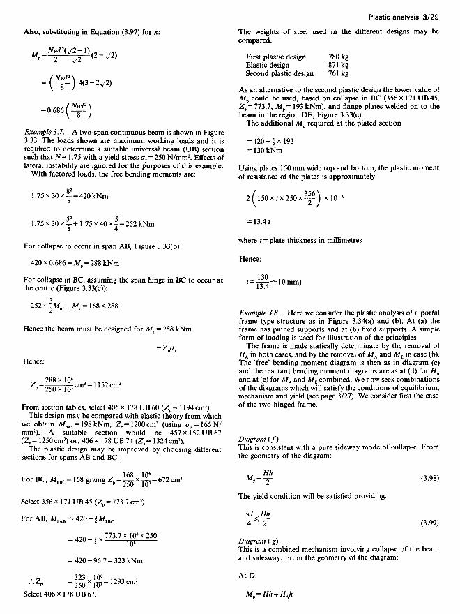
Also, substituting in Equation (3.97) for x:

«,,^V2zl)(2-V2)

-(Uf)O-U*

-«•(*£)

Example 3.7. A two-span continuous beam is shown in Figure3.33. The loads shown are maximum working loads and it isrequired to determine a suitable universal beam (UB) sectionsuch that N= 1.75 with a yield stress ay = 250 N/mm2. Effects oflateral instability are ignored for the purposes of this example.

With factored loads, the free bending moments are:

1.75 x 30 x ̂ = 420 kNmO

1.75 x 30 x ̂ +1.75 x 40 x I = 252 kNm

For collapse to occur in span AB, Figure 3.33(b)

420 x 0.686 = Mp = 288 kNm

For collapse in BC, assuming the span hinge in BC to occur atthe centre (Figure 3.33(c)):

252 = ~Mp, Mp=168<288

Hence the beam must be designed for Mp = 288 kNm

-v,Hence:

_ 288 x l O 6 , t , M ,Zp = 250MO^Cm H52cm

From section tables, select 406 x 178 UB 60 (Zp = 1194cm3).This design may be compared with elastic theory from which

we obtain Afmax= 198 kNm, Z6= 1200 cm3 (using <rw=165N/mm2). A suitable section would be 457x152 UB 67(Ze= 1250cm3) or, 406 x 178 UB 74 (Z6 = 1324cm3).

The plastic design may be improved by choosing differentsections for spans AB and BC:

For BC, MPBC = 168 giving Zp = i|j x I?! = 672 cm3

Select 356 x 171 UB 45 (Zp = 773.7 cm3)

For AB, MPAB = 420 - iMPBC

= 420- jx773-7 ̂ 250

= 420-96.7 = 323 kNm

•••ZP =§xw=1293cm3

Select 406 x 178 UB 67.

The weights of steel used in the different designs may becompared.

First plastic design 780 kgElastic design 871 kgSecond plastic design 761 kg

As an alternative to the second plastic design the lower value ofMp could be used, based on collapse in BC (356 x 171 UB 45,Zp= 773.7, Mp= 193 kNm), and flange plates welded on to thebeam in the region DE, Figure 3.33(c).

The additional Mp required at the plated section

= 420-|xl93= 130 kNm

Using plates 150mm wide top and bottom, the plastic momentof resistance of the plates is approximately:

2^150xrx250x^^ x lO- 6

= 13.4/

where / = plate thickness in millimetres

Hence:

t — -yr-7 —10 mm)

Example 3.8. Here we consider the plastic analysis of a portalframe type structure as in Figure 3.34(a) and (b). At (a) theframe has pinned supports and at (b) fixed supports. A simpleform of loading is used for illustration of the principles.

The frame is made statically determinate by the removal of//A in both cases, and by the removal of MA and ME in case (b).The 'free' bending moment diagram is then as in diagram (c)and the reactant bending moment diagrams are as at (d) for //Aand at (e) for MA and ME combined. We now seek combinationsof the diagrams which will satisfy the conditions of equilibrium,mechanism and yield (see page 3/27). We consider first the caseof the two-hinged frame.

Diagram (/)This is consistent with a pure sideway mode of collapse. Fromthe geometry of the diagram:

Mp = f (3.98)

The yield condition will be satisfied providing:

vW HhT^ 2 (3.99)

Diagram (g)This is a combined mechanism involving collapse of the beamand sidesway. From the geometry of the diagram:

AtD:

M9 = HhT^HJi

Figure 3.34

AtC:

*>•¥-%***

Adding:

**-?+?

or:

M=™+™p 8 4 (3.100)

In the case of the frame with fixed feet, there are three possible

modes of collapse. The corresponding bending moment dia-grams are constructed at (h), (j) and (k) and the results are asfollows:

Diagram (h):

M-H*hM,-^rMp = HH-HAh-Mf

Hence:

J-UiMp = — (3.101)

Diagram (J):

., Wl Hh^11.M,=-f—T±H*h

Mp = Hh + HAh-Mp

Adding:

M(4-Wl+Hh3A*P-^- + ̂

or:

^1T+T* (3J02)

Diagram (k)This mode is the same as the collapse of a fixed end beam; thecolumns are not involved in the collapse apart from providingthe resisting moment Mp at B and D. From the geometry of thediagram:

^P = X (3*103)

Example 3.9. Here we consider a pitched roof frame, a struc-ture which is eminently suitable for design by plastic methods.The frame is shown in Figure 3.35(a). The given loads arealready factored and we are to find the required section moduluson the basis of a yield-stress ay = 280 N/mm2, neglecting instabi-lity tendencies and the reduction in plastic moment of resistancedue to axial forces.

The bending moment diagram at collapse is shown in Figure3.35(b). The free bending moment diagram, EFGB, is drawn toscale after evaluating values of moment at intervals along therafter members. The reactant line (#A diagram) is then drawn bytrial and error so that the maximum moment in the region BC isequal to the moment at D. This moment is the required Mp forthe frame and is found to be:

A/p = 52kNm = (7yZp

from which:

_ 52x l0 3 xl0 3 3

Z'= 280 x lO 3 =186cm

Home8 and Baker and Heyman9 should be consulted for a more

Figure 3.35

detailed study of plastic analysis. Among the topics deserving offurther study are:

(1) Use of the principle of virtual work in obtaining relation-ships between applied loads and plastic moments of resis-tance.

(2) Effects of strain hardening.(3) Evaluation of shape factors for various cross-sections.(4) Application of the maximum principle in obtaining lower

bounds.

(5) Numbers of independent mechanisms.(6) Shakedown.(7) Effects of axial forces.(8) Moment carrying capacity of columns.(9) Behaviour of welded connections.

References

1 Jenkins, W. M (1982) Structural mechanics and analysis level IV7 V.Thomas Nelson/Van Nostrand Reinhold, London.

2 Coates, R. C., Coutie, M. G. and Kong, F. K. (1972) Structuralanalysis. Nelson, London.

3 Ghali, A. and Neville, A. M. (1978) Structural analysis. 2nd edn.Chapman and Hall, London.

4 Zeinkiewicz, O. C. (1977) The finite element method. McGraw-Hill,Maidenhead.

5 Desai, C. S. (1977) Elementary finite element methods.Prentice-Hall, New Jersey.

6 PAFEC (1978) PAFEC 75, Pafec Ltd, Pafec House, 40 Broadgate,Beeston, Nottingham NG9 2FW.

7 Warburton, G. B (1976) The dynamical behaviour of structures,2nd edn. Pergamon Press, Oxford.

8 Home, M. R. (1979) Plastic theory of structures, 2nd edn.Pergamon Press, Oxford.

9 Baker, J. and Heyman, J. (1969) Plastic design of frames.Cambridge University Press, Cambridge.

Bibliography

Bhatt, P. (1981) Problems in structural analysis by matrix methods. TheConstruction Press, London.

Cheung, Y. K. (1976) Finite strip method in structural analysis.Pergamon Press, Oxford.

Cheung, Y. K. and Yeo, M. F. (1979) A practical introduction to finiteelement analysis. Pitman, London.

Dawe, D. J. (1984) Matrix and finite element displacement analysis ofstructures. Clarendon Press, Oxford.

Graves Smith, T. R. (1983) Linear analysis of frameworks. EllisHorwood, Chichester.

Harrison, H. B. (1980) Structural analysis and design: somemini-computer applications. Pergamon Press, Oxford.

Jenkins, W. M., Coulthard, J. M. and de Jesus, G. C. (1983) BASICcomputing for civil engineers. Van Nostrand Reinhold, London.

McGuire, W. and Gallagher, R. H. (1979) Matrix structural analysis.Wiley, Chichester.