arX

iv:1

511.

0599

8v1

[co

nd-m

at.d

is-n

n] 1

8 N

ov 2

015

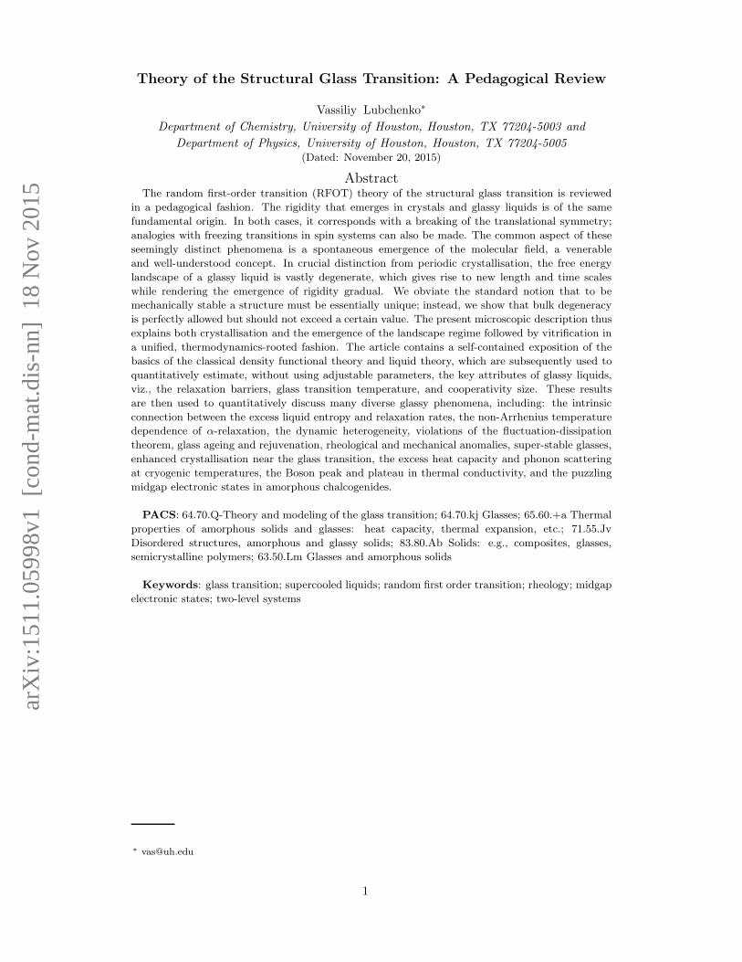
Theory of the Structural Glass Transition: A Pedagogical Review

Vassiliy Lubchenko∗

Department of Chemistry, University of Houston, Houston, TX 77204-5003 and

Department of Physics, University of Houston, Houston, TX 77204-5005

(Dated: November 20, 2015)

AbstractThe random first-order transition (RFOT) theory of the structural glass transition is reviewed

in a pedagogical fashion. The rigidity that emerges in crystals and glassy liquids is of the same

fundamental origin. In both cases, it corresponds with a breaking of the translational symmetry;

analogies with freezing transitions in spin systems can also be made. The common aspect of these

seemingly distinct phenomena is a spontaneous emergence of the molecular field, a venerable

and well-understood concept. In crucial distinction from periodic crystallisation, the free energy

landscape of a glassy liquid is vastly degenerate, which gives rise to new length and time scales

while rendering the emergence of rigidity gradual. We obviate the standard notion that to be

mechanically stable a structure must be essentially unique; instead, we show that bulk degeneracy

is perfectly allowed but should not exceed a certain value. The present microscopic description thus

explains both crystallisation and the emergence of the landscape regime followed by vitrification in

a unified, thermodynamics-rooted fashion. The article contains a self-contained exposition of the

basics of the classical density functional theory and liquid theory, which are subsequently used to

quantitatively estimate, without using adjustable parameters, the key attributes of glassy liquids,

viz., the relaxation barriers, glass transition temperature, and cooperativity size. These results

are then used to quantitatively discuss many diverse glassy phenomena, including: the intrinsic

connection between the excess liquid entropy and relaxation rates, the non-Arrhenius temperature

dependence of α-relaxation, the dynamic heterogeneity, violations of the fluctuation-dissipation

theorem, glass ageing and rejuvenation, rheological and mechanical anomalies, super-stable glasses,

enhanced crystallisation near the glass transition, the excess heat capacity and phonon scattering

at cryogenic temperatures, the Boson peak and plateau in thermal conductivity, and the puzzling

midgap electronic states in amorphous chalcogenides.

PACS: 64.70.Q-Theory and modeling of the glass transition; 64.70.kj Glasses; 65.60.+a Thermal

properties of amorphous solids and glasses: heat capacity, thermal expansion, etc.; 71.55.Jv

Disordered structures, amorphous and glassy solids; 83.80.Ab Solids: e.g., composites, glasses,

semicrystalline polymers; 63.50.Lm Glasses and amorphous solids

Keywords: glass transition; supercooled liquids; random first order transition; rheology; midgap

electronic states; two-level systems

∗ vas@uh.edu

1

CONTENTS

I. Motivation 3

II. Placing the Glass Transition on the Map, Thermodynamics-wise: The

Microcanonical Spectrum of Liquid, Supercooled-Liquid, and Crystal States. The

Definition of the Glass Transition and Ageing 7

III. Liquid-to-crystal transition as a breaking of translational symmetry. Review of

the Theory of Liquids and Liquid-to-Solid Transition. 11

A. What drives crystallisation, why it is a discontinuous transition, and why the

entropy of fusion is modest 11

B. Emergence of the Molecular Field 24

C. Transferability of DFT results from model liquids to actual compounds 36

IV. Emergence of Aperiodic Crystal and Activated Transport, as a Breaking of

Translational Symmetry 40

A. The Random First Order Transition (RFOT) 40

B. Configurational Entropy 49

C. Qualitative discussion of the transition at TA as a kinetic arrest, by way of

mode-mode coupling. Connection between kinetic and thermodynamic views

on the transition at TA. Short discussion on colloids, binary and metallic

mixtures, and ionic liquids. 55

D. Connection with spin models 58

V. Quantitative Theory of Activated transport in Glassy Liquids 64

A. Glassy liquid as a mosaic of entropic droplets 64

B. Mismatch Penalty between Dissimilar Aperiodic Structures: Renormalisation

of the surface tension coefficient 73

C. Quantitative estimates of the surface tension, the activation barrier for liquid

transport, and the cooperativity size 78

VI. Dynamic heterogeneity 94

A. Correlation between non-exponentiality of liquid relaxation and fragility 95

B. Violation of the Stokes-Einstein relation and decoupling of various processes 97

VII. At the crossover from collisional to activated transport 101

VIII. Relaxations far from equilibrium: glass ageing and rejuvenation 109

A. Ageing 110

B. Rejuvenation 113

IX. Rheological and Mechanical Anomalies 115

A. Shear thinning 115

B. Mechanical Strength 118

X. Ultra-Stable Glasses 119

XI. Ultimate Fate of Supercooled Liquids 122

XII. Quantum Anomalies 124

A. Two-Level Systems and the Boson Peak 125

B. The midgap electronic states 133

2

XIII. Summary and Connection with Jammed and Other Types of Aperiodic Solids 141

A. Volume mismatch during ageing 148

References 150

I. MOTIVATION

Practical use of structural glasses by early hominins—in the form of tools and weapons—

likely goes back to about 2 million years ago [1] and thus well predates the appearance

of the anatomically modern human. The lack of crystallite boundaries, which helped our

forefathers to impart sharp and smooth edges to obsidian rocks, still underlies many uses

of structural glasses. For instance, it results in optical transparency and mechanical stur-

diness of amorphous silicates; the combination of the two makes glasses uniquely useful in

construction and in information technology. Metallic glasses are exceptionally rigid at room

temperature while being soft and malleable over a rather broad temperature range near the

glass transition [2]. In contrast, polycrystalline metals liquefy almost instantly near their

melting temperature and thus have a much narrower processing window. Some of the ap-

plications of glasses are thoroughly modern: The reflectivity and electrical conductance of

chalcogenide alloys depend on whether the material is in a crystalline or amorphous form,

a property currently utilised in optical drives. In some of these alloys, crystal-to-glass tran-

sition can be induced by electric current or irradiation, which can be exploited to make

non-volatile computer memory and for other useful applications [3–9].

The relatively gradual onset of rigidity in structural glassformers—viewed alternatively

as a rapid, super-Arrhenius slowing down of molecular motions with increasing density

or lowering temperature—is as useful to the industrial designer as it is interesting to the

physicist and chemist. For basic symmetry reasons, liquids freeze into periodic crystals in a

discontinuous fashion so that shear resistance emerges within a narrow temperature interval.

The mechanical stability of a periodic array of atoms is intuitive to those familiar with the

Debye theory: The positive-definiteness of the force-constant matrix for a periodic lattice

can be readily shown for a variety of generic force laws between individual atoms [10].

Even in those difficult cases where the individual interactions balance each other out in

a delicate fashion—such situations often arise in applications such as multiferroics—the

stability analysis of a periodic crystal usually reduces to that for a very small number of

normal modes. In contrast, the structure and rigidity change continuously on approach

to vitrification, while there is no obvious way to diagonalise the force-constant matrix for

an aperiodic lattice. Another way to look at this distinction is that glassy liquid and the

corresponding crystal, if any, occupy distinct regions in the phase space that are separated

by a substantial barrier. The glass transition itself is not even a phase transition but,

rather, signifies that the supercooled liquid falls out of equilibrium, an expressly kinetic

phenomenon. Glasses are typically only metastable with respect to crystallisation.

Given the above notions, it appears reasonable to question whether the underlying causes

of rigidity in periodic crystals and glasses are related even as the local interactions in the

two types of solids are very similar, aside from subtle differences in bond lengths and angles.

In such a view, the roles of the cohesive forces and the thermodynamic driving force for

solidification are essentially gratuitous; the cohesive forces simply prevent the particles from

flying apart and/or fix local coordination on average. To avoid confusion, we note that in

liquids made of rigid particles, there is no actual bonding and so one speaks of contacts or

collisions. Nevertheless, the thermodynamics of packing-driven solidification can be put in

correspondence with that of chemically-bonded solids, as will be discussed.

As surprising and unpalatable it may feel, the view of a gratuitous role of thermodynamics

3

in glassy phenomena would seem to be suggested by a number of theoretical developments.

For instance, one of the earliest methodologies that yielded an emergence of rigidity in ape-

riodic systems was the mode-coupling theory (MCT) [11, 12]. Hereby the rigidity arises for

expressly kinetic reasons: At sufficiently high densities, a particle can not keep up with the

feedback it receives from the surrounding particles in response to its own motions. To reduce

the feedback, the particle is forced to slow down. In the mean-field limit of the MCT, in

which equations become tractable, the slowing down is nothing short of catastrophic; it leads

to a complete kinetic arrest and, hence, freezing. A thermodynamic signature of this type

of freezing, if any, does not readily transpire in this framework. A variety of models charac-

terised by complicated kinetic constraints have been conceived in the past few years [13, 14],

motivated by Palmer et al.’s work on hierarchically constrained dynamics [15]. The latter

models, like the MCT, were advanced in the early 80s. These kinetics-based models exhibit a

slowing down of cooperative nature, and so does the MCT. Complicated kinetic phenomena,

which are at least superficially similar to the non-Arrhenius and non-exponential relaxations

observed in actual glass-formers, can emerge in kinetically constrained models even if the

thermodynamics of the model are trivial [16].

A distinct set of models suggesting a somewhat gratuitous role of thermodynamics in the

structural glass transition focus on the phenomenon of jamming [17–20]. During jamming,

as epitomised by sand dunes, the thermal motions are negligible because temperature is

effectively zero compared to the energies involved. In apparent similarity to glasses, the

rigidity of jammed systems appears to form gradually. Flow occurs through the proliferation

of soft, harmonic modes that arise when particle contacts are removed. Such soft modes

also emerge in random matrix theories [21] and have been implicated as giving rise to the so

called Boson Peak. The Boson Peak is a set of vibrational-like states in glasses at frequencies

of 1 THz or so, which reveals itself as a “bump” in the heat capacity and excess phonon

scattering at the corresponding temperatures, i.e., near 101 K [22, 23].

Yet we shall see in the following that one is, in fact, correct in expectating that thermody-

namics are not simply a spectator of the slowing down that takes place in supercooled liquids

when they are cooled or compressed toward the glass transition. Until vitrification has taken

place, the liquid is in fact equilibrated and thus should obey detailed balance [24, 25]. (The

liquid is equilibrated conditionally in that there is a lower free energy state, viz., the crystal.

The latter, however, is behind a barrier and is not accessed.) By detailed balance, coopera-

tive motions that give to rise to the non-trivial kinetics observed in supercooled liquids must

correspond to a specific set of microstates. Such states necessarily have a thermodynamic

signature in the form of additional entropy and heat capacity. For instance, the critical

slowing down during a second order transition corresponds to a non-analyticity in the free

energy [26], thus leading to a singularity in the temperature dependence of the heat capacity.

Detailed balance dictates that a complete theory of the slowing down in supercooled liquids

must describe both the thermodynamics and kinetics in an internally consistent, unified

fashion. The present review is intended as a pedagogical exposition of a theory that delivers

exactly that: a unified, quantitative description of thermodynamic and kinetic phenomena

in supercooled liquids and glasses. This theory is called the random first order transition

(RFOT) theory and has been developed since the early-mid 80s, earlier reviews can be found

in Refs. [23, 27, 28]. The theory has provided a microscopic framework that allows one to

understand the emergence of rigidity in aperiodic systems in thermodynamic terms and thus

connect the structural glass transition to a better understood—at least conceptually—fields

of the liquid-to-crystal transition and the theory of chemical bonding in solids [29].

Despite showing basic similarity in bonding, supercooled liquids and glasses differ funda-

mentally from periodic crystals in that they are vastly structurally degenerate, that is, their

free energy exhibits exponentially many minima at a specific value of the free energy. The

thermodynamic signature of the degeneracy is the excess liquid entropy of the supercooled

4

liquid relative to the corresponding crystal. Upon vitrification, this excess entropy ceases

to change as the temperature lowers, thus leading to a discontinuity in the measured heat

capacity. The remarkable variety of relaxations unique to glassy systems can all be traced

to transitions between the distinct free energy minima. This microscopic picture gives rise

to quantitative predictions for many signature phenomena that accompany the structural

glass transition and their quantitative characteristics, without using adjustable parameters.

These cardinal predictions of the theory include the activation barriers for α-relaxation and

their relation to the excess liquid entropy [30, 31] and elastic constants [32–34], details of

the deviations from Arrhenius behaviour [31, 35, 36] and the pressure dependence of the

barriers. [37] In addition, the theory predicts correlations of thermodynamics with non-

exponential relaxations [38], the cooperativity length [31, 33], deviations from the Stokes-

Einstein relation [39], ageing dynamics in the glassy state [40], crossover between activated

and collisional transport in glass-forming liquids [35, 41, 42], decoupling between various

types of relaxation [43], beta-relaxation [44], shear thinning [45], dynamics near the surface

of glasses [46], mechanical strength [47], rejuvenation and front propagation in ultrastable

glasses [48, 49], and re-entrant T -dependence of the crystallisation rate [50].

The RFOT theory is a microscopic theory: For simple liquids, such as hard spheres or

Lennard-Jones particles, the theory starts from the functional form of the interaction and

provides a detailed approach to compute every quantity of interest from scratch. For the

more complicated glass-forming materials of technology, the interactions must be evaluated

by quantum-chemical means. Owing to the computational complexity of the quantum-

chemical problem, detailed results cannot be expressed in closed form. In these cases,

the microscopic analysis of the RFOT theory delineates a small sufficient set of system-

specific quantities—structural and thermodynamic—that represent the microscopic input

for computations of the dynamics. These quantities can be extracted by measurement, such

as X-ray scattering, the Brillouin scattering, and the calorimetry of the liquid-to-crystal

transition, while no phenomenological assumptions are made. The ensuing computations

do not involve adjustable parameters, consistent of course with the microscopic nature of

the description. Importantly, none of those listed measurements have to do directly with

the glass transition per se or use any kind of dynamic assumptions.

Likewise, the RFOT theory has elucidated in a microscopic fashion several quantum phe-

nomena, [28] which play a role at cryogenic temperatures. Somewhat surprisingly, the low

temperature physics turns out to be intrinsically related to the molecular motions that froze

in at the much higher, glass transition temperature. The theory ineluctably leads to the

result that an equilibrated liquid must have a specific, rather universal concentration of con-

figurations that originate from the transition state configurations for transport. In the equi-

librated liquid, these special configurations are “domain walls” of high free energy density

separating compact regions characterised by relatively low free energy density. The domain

walls quantitatively account for the excess structural states in cryogenic glasses responsible

for the mysterious two-level systems and the Boson Peak [22, 23, 51, 52]. More recently,

it has been established that the domain walls have a topological signature in chalcogenide

alloys and host very special midgap electronic states, responsible for light-induced midgap

absorption and ESR signal [53, 54]. These quantum phenomena underscore the danger of

thinking of crystals merely as some kind of disordered analogue of periodic crystals. Again,

we shall use thermodynamics as our guiding light in elucidating this important feature of

structural glasses.

Consistent with its being firmly rooted in thermodynamics, the RFOT theory highlights

the symmetry aspects of the structural glass transition. The basic symmetry that becomes

broken en route to the glass transition is the translational symmetry intrinsic to liquids

and gases. As a result of this symmetry breaking, the one-particle density profile (gradu-

ally) switches from being, in time average, spatially uniform to a sensibly fixed collection of

5

disparate, sharp peaks. Similarly to periodic crystals, these peaks indicate the particles or-

ganise themselves into structures that live much longer than the vibrations. In contrast with

periodic crystals, however, the structures are not infinitely long-lived but eventually recon-

figure, thus leading to a liquid flow on long times that eventually restores the translational

symmetry. Only when the activated reconfigurations become slower than the quenching

rate, which depends on glass preparation, does the system fall out of equilibrium com-

pletely. Importantly, translational symmetry being broken does not imply there is another

symmetry, like periodic ordering, that replaces it. The symmetry perspective furnishes the

requisite completeness we have come to associate with established physical theories, such

as the theory of second order transitions, which was originally built on a symmetry-based

coarse-grained functional [55] and was later complemented by the discovery of anomalous

scaling. The latter is fully determined by the symmetry and range of the molecular inter-

action but not its detailed form [26]. Likewise, the presence of an underlying symmetry

breaking makes the RFOT description of the structural glass transition robust with respect

to possible ambiguities that inevitably arise from approximations and incomplete knowledge

of detailed particle-particle interactions; it thus undergirds the applicability of the theory

to rigid particles and chemically-bonded liquids alike. The symmetry perspective will also

allow us to connect the glass transition with the phenomenon of jamming.

The RFOT theory definitively answers the aforementioned basic question as to the me-

chanical stability of an aperiodic array of particles: To achieve macroscopic mechanical

stability on a finite time scale, the structure does not have to be unique; indeed, even

a thermodynamic degeneracy is perfectly allowed so long as it does not exceed a certain

value. In turn this guarantees that the transitions between alternative free energy minima

are sufficiently slow. Relics of locallymetastable configurations are present in the frozen glass

and persist down to the lowest temperatures measured but do not affect the macroscopic

stability.

The article is intended to be a rather self-contained source on the foundations of the

RFOT theory and on how to obtain its main results with a minimum of technical complex-

ity. The narrative is organised as follows: Section II describes what the glass transition is

from the viewpoint of macroscopic thermodynamics and explains the relation between the

supercooled-liquid/glass states and the thermodynamically stable liquid and crystal states.

Section III explains the thermodynamics of the ordinary liquid-to-periodic-crystal transi-

tion and, along the way, introduces the basic machinery of the classical density theory and

the theory of liquids, which will be our main tools in discussing things glassy. These tools

no longer seem to be part of standard courses in statistical mechanics; it is hoped that

the present text covers the necessary minimum in a sufficiently self-contained manner. Sec-

tion IV uses the machinery from Section III to understand the emergence of aperiodic solids,

from both the thermodynamic and kinetic perspectives. There we also briefly discuss the

connections with several spin models; these connections have proved to be a source of both

insight and some confusion to many over the years. In Section V, we establish in a self-

contained manner both the qualitative and quantitative features of activated transport and

the intrinsic, testable predictions that connect the thermodynamics and kinetics of glassy

liquids. These results will be used in Sections VI-XII to review quantitative predictions

made by the RFOT theory on a great variety of glassy phenomena mentioned above. In

Section XIII, we summarise, briefly review the formal status of the theory and establish an

intrinsic connection and, at the same time, basic distinction between the glass transition

and jamming.

Last but not least, let us settle a semantic issue that can be confusing to physicists and

chemists alike, in the author’s experience: We will often use the words “aperiodic crystal”

and “aperiodic lattice”—or simply “lattice”—when referring to the infinite aperiodic array

of particles that a glass or a snapshot of a liquid is. The purpose is to avoid the repeated use

6

B 1 K

/T1 g

Kauzmann temperature

( = const)VHE

p( = const)

activated transport collisional transportVXtal VliqV

Xtal liq

0.8k /T

Xtal

for Xtal−liquidtransition

/T1 m

temperatureglass transition

temperaturemelting

Liquid

Dulong−Petit

S, entropyper particle

A

V

mp

transition inisobaric ensemble

transition inisochoric ensemble

Liquid

Xtal

(a) (b)

T( = const)

tangent construction

gla

ssy

sta

tes

H

cro

sso

ver

latent heatenthalpy (energy) "gap"

S

S

fusi

on

en

tro

py

Xtal

liq

H

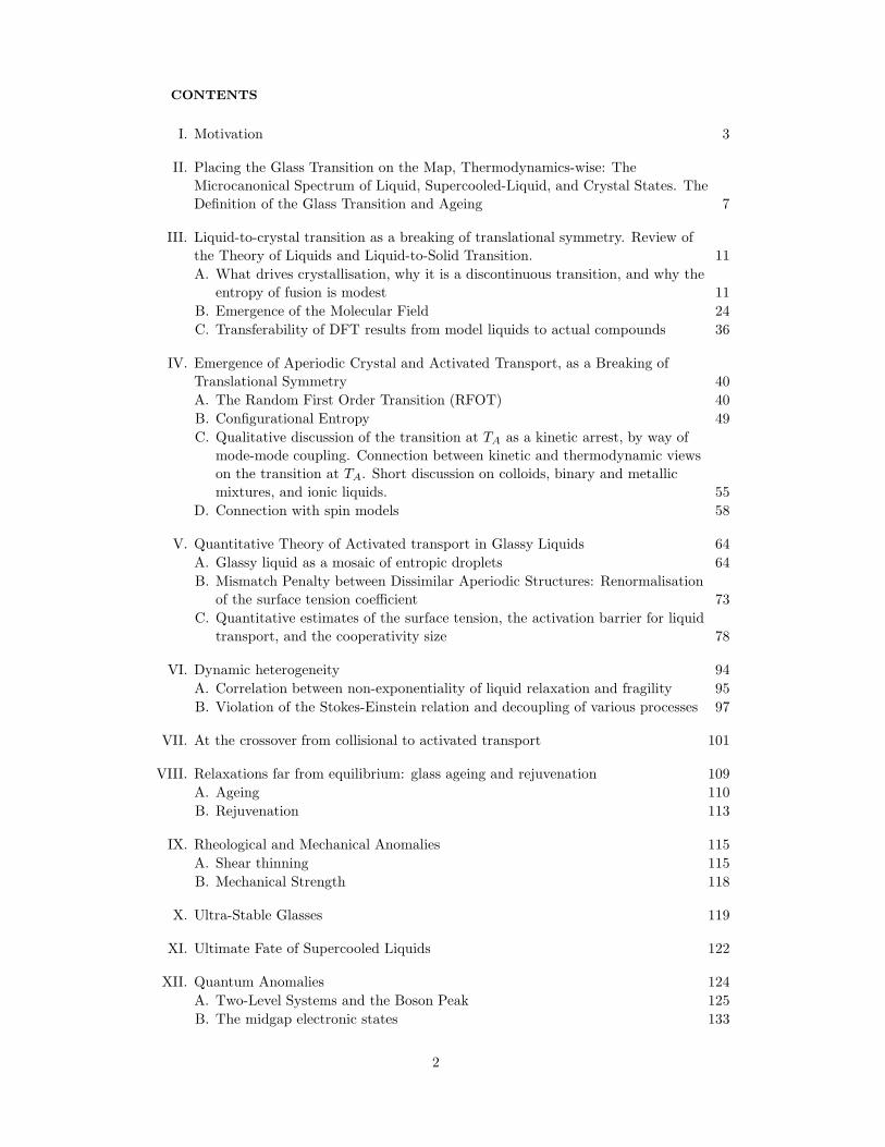
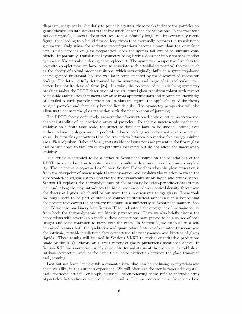
FIG. 1. (a) The “spectrum” of a liquid in the enthalpy (energy) range of relevance to the liquid-

to-crystal and the glass transition. The thick, solid black lines depict the entropy as a function

of enthalpy; the high and low enthalpy branches correspond to the liquid and crystal respectively.

The states between HXtal and Hliq are bypassed during crystallisation but are visited, if the liquid

can be supercooled below the melting temperature. (Some degree of supercooling is necessary

for crystallisation to proceed anyways because crystal-nucleation is subject to a barrier.) The

glass transition ordinarily occurs at enthalpy values within the enthalpy gap [HXtal,Hliq], when

the liquid excess entropy is 0.8 . . . 0.9 kB or so, per rigid molecular unit. The crossover to the

landscape regime (“glassy states”) could be either above or below the melting point Tm, the two

cases corresponding to strong and fragile liquids respectively. (b) The two thick solid curves

correspond to the Helmholtz free energy of two phases characterised by distinct density, such as

liquid and crystal. The equilibrium transition between the two phases occurs at pressure p = pm. It

is, in principle, possible to transition between the two phases by forcing the system to stay spatially

uniform and remain on the branch corresponding to the current phase up to the crossing point V ‡

and then switch to the other phase as a whole. However, the two phases will not be in mechanical

equilibrium during the transition, −(∂Aliq/∂V )T |V ‡ 6= −(∂AXtal/∂V )T |V ‡ .

of the awkward “infinite aperiodic array.” (The author recognises that in their traditional

use, the words “crystal” and “lattice” usually refer to periodic arrays of objects.)

II. PLACING THE GLASS TRANSITION ON THE MAP, THERMODYNAMICS-

WISE: THE MICROCANONICAL SPECTRUM OF LIQUID, SUPERCOOLED-

LIQUID, AND CRYSTAL STATES. THE DEFINITION OF THE GLASS TRANSI-

TION AND AGEING

We begin by locating the supercooled-liquid state on the energy landscape of the system,

as reflected in its microcanonical spectrum. Fig. 1(a) schematically shows the log-density of

states, or entropy S, as a function of energy E, if the experiment is done at constant volume

V , or enthalpy H , if one employs the more common isobaric conditions p = const. Note

the latter is the ensemble of choice for infinitely rigid particles, which do not undergo phase

changes at constant volume because their equation of state is simply p/T = f(V ), where

f(V ) is a function of volume. The two (disconnected) thick solid lines correspond to the

periodic crystal states at low enthalpies and the liquid (and gas) states at high enthalpies.

The slope of each curve is equal to the inverse temperature at the corresponding value of

the enthalpy: 1/T = (∂S/∂H)p = (∂S/∂E)V .

In Fig. 1(a), the spectral region bounded by the points on the curves through which

the common tangent passes is special (these points are shown as large red dots). The

7

states belonging to this special spectral region are bypassed during crystallisation and may

thus be said to comprise an enthalpy or energy “gap” because they are inaccessible in true

equilibrium. For an enthalpy value falling within the gap, the system is phase-separated into

liquid and crystal, while the total entropy is a linear function of the enthalpy and simply

reflects the partial quantity of the liquid and crystal, an instance of the lever rule [56]:

S(H) = xSliq+(1−x)SXtal, where H = xHliq+(1−x)HXtal and x is the mole fraction of the

liquid. The quantities Sliq and SXtal are the entropies at the the edges of the enthalpy gap,

viz., Hliq and HXtal respectively. The numerical value of the width of the gap, (Hliq−HXtal),

which is equal to the latent heat, can be divided by the melting temperature Tm to obtain

the entropy of fusion Sm = Sliq − SXtal. The latter is generically about 1.5kB per particle

for ionic compounds [57]; it is somewhat larger for Lennard-Jones-like substances (1.68kBfor Ar [56]) but often less than kB for covalently bonded liquids, such as SiO2 [57]. The

corresponding enthalpy of fusion is thus comparable to the kinetic energy of the atoms.

If, however, the cooling rate is finite, the liquid must be supercooled somewhat before

it can crystallise, because the nucleation barrier for crystallisation is infinite strictly at the

melting temperature. Consequently, the liquid states on the right flank of the enthalpy gap

are sampled. These states correspond to a supercooled liquid. Note the higher the viscosity,

the larger the width of the sampled region, because the prefactor of the nucleation rate

scales roughly inversely with the viscosity.

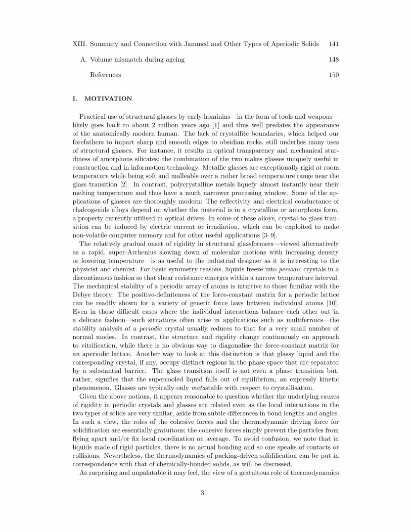
Now, it is often the case that the viscosity and, thus, the relaxation times grow rapidly

with lowering the temperature, see Fig. 2; the details of the viscosity growth and the relation

between viscosity and relaxation rates will be discussed in detail shortly. Given such an in-

crease in the relaxation time, a liquid is often easy to bring to and maintain in a supercooled

state. A familiar household example of such a supercooled liquid is glycerol, which is rather

difficult to crystallise, as it turns out. (See, however, Onsager’s anecdote about a glycerol

factory in Canada [58].) One can continue to cool down such a deeply supercooled liquid at

a slow rate, with little risk of crystallisation. Eventually, a liquid cooled at a steady rate will

fail to reach equilibrium—owing to the rapidly growing relaxation times. This statement

applies at least to the slow rates realistically achievable in the laboratory; Stevenson and

Wolynes have argued given a slow enough cooling rate, a (periodic-crystal-forming) liquid

will actually crystallise [50]. The re-entrant behaviour the glass-to-crystal nucleation, which

has been recently observed in some organic liquids, [59, 60] seems to be consistent with this

prediction, see Section XI.

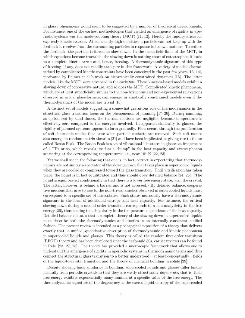
The structural relaxation responsible for the viscous flow can be readily witnessed in the

form of a low-frequency peak in the dielectric loss spectrum ǫ′′(ω). This relatively slow

process is traditionally called α-relaxation. Other, faster processes can be argued to take

place in addition to main α-relaxation; these faster processes are often non-Arrhenius as

well, see Fig. 3.

Once the liquid that is being cooled fails to equilibrate, we say that the glass transition,

or vitrification, has taken place, at a temperature Tg. Although the system is no longer

equilibrated, the particles continue to move and the material still relaxes partially, which

is called “ageing.” These relaxational motions are even slower than the motions above the

glass transition, whose sluggishness caused the falling out of equilibrium in the first place;

the deeper the quench below the glass transition, the slower the ageing.

The non-equilibrium, glassy states are no longer identifiable on the equilibrium spectrum

in Fig. 1. Rather, they are a complicated mixture of configurations that are similar to

structures equilibrated in a continuous range of temperatures; these are sometimes called

“fictive” temperatures. Still, before significant ageing has taken place, the structure of the

glass is very close to that of the supercooled liquid just above the glass transition, save for

the somewhat reduced magnitude of vibrational motions. Hereby, the fictive temperature is

only weakly distributed and approximately equal to the glass transition temperature itself.

8

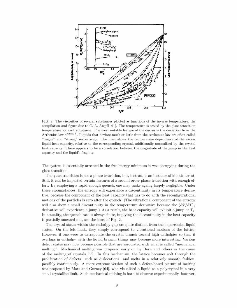
FIG. 2. The viscosities of several substances plotted as functions of the inverse temperature, the

compilation and figure due to C. A. Angell [61]. The temperature is scaled by the glass transition

temperature for each substance. The most notable feature of the curves is the deviation from the

Arrhenius law econst/T . Liquids that deviate much or little from the Arrhenius law are often called

“fragile” and “strong” respectively. The inset shows the temperature dependence of the excess

liquid heat capacity, relative to the corresponding crystal, additionally normalised by the crystal

heat capacity. There appears to be a correlation between the magnitude of the jump in the heat

capacity and the liquid’s fragility.

The system is essentially arrested in the free energy minimum it was occupying during the

glass transition.

The glass transition is not a phase transition, but, instead, is an instance of kinetic arrest.

Still, it can be imparted certain features of a second order phase transition with enough ef-

fort. By employing a rapid enough quench, one may make ageing largely negligible. Under

these circumstances, the entropy will experience a discontinuity in its temperature deriva-

tive, because the component of the heat capacity that has to do with the reconfigurational

motions of the particles is zero after the quench. (The vibrational component of the entropy

will also show a small discontinuity in the temperature derivative because the (∂V/∂T )pderivative will experience a jump.) As a result, the heat capacity will exhibit a jump at Tg.

In actuality, the quench rate is always finite, implying the discontinuity in the heat capacity

is partially smeared out, see the inset of Fig. 2.

The crystal states within the enthalpy gap are quite distinct from the supercooled-liquid

states. On the left flank, they simply correspond to vibrational motions of the lattice.

However, if one were to extrapolate the crystal branch toward high enthalpies so that it

overlaps in enthalpy with the liquid branch, things may become more interesting: Various

defect states may now become possible that are associated with what is called “mechanical

melting.” Mechanical melting was proposed early on by Born and others as the cause

of the melting of crystals [63]. In this mechanism, the lattice becomes soft through the

proliferation of defects—such as dislocations—and melts in a relatively smooth fashion,

possibly continuously. A more extreme version of such a defect-based picture of melting

was proposed by Mott and Gurney [64], who visualised a liquid as a polycrystal in a very

small crystallite limit. Such mechanical melting is hard to observe experimentally, however,

9

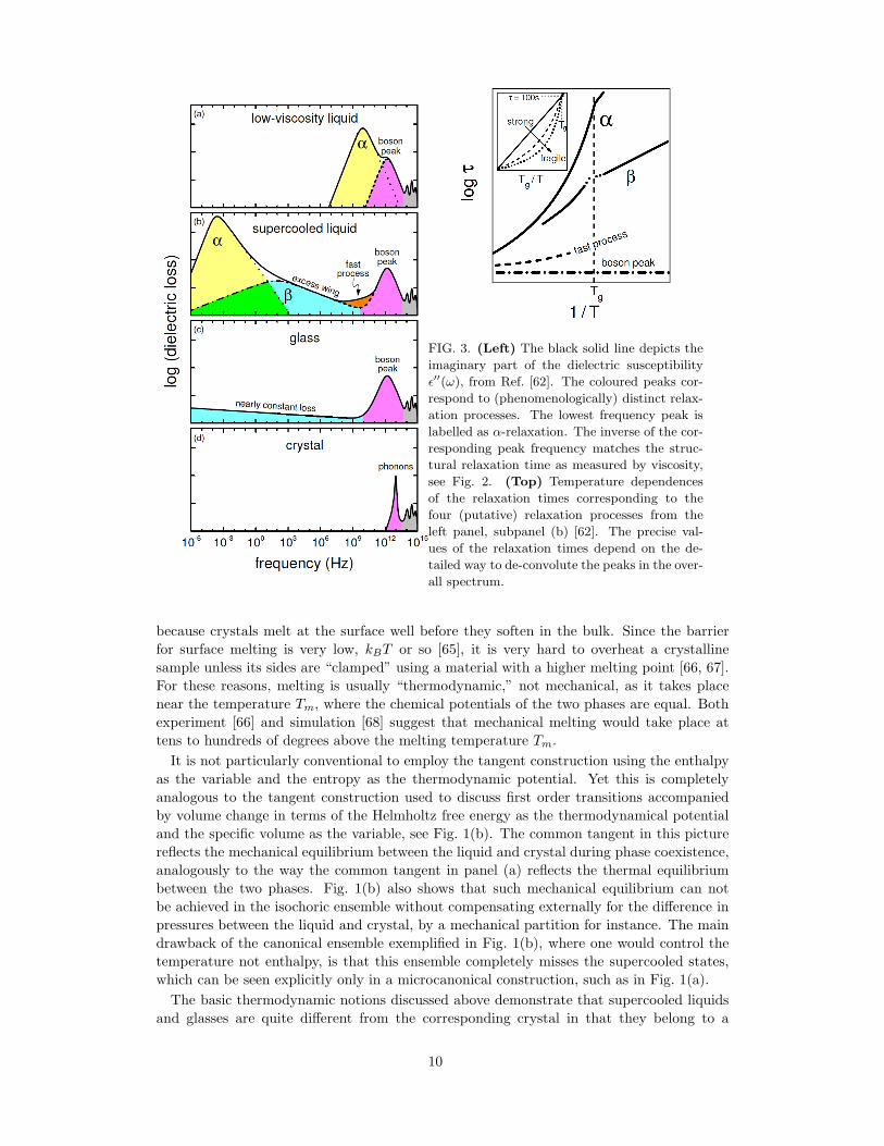
FIG. 3. (Left) The black solid line depicts the

imaginary part of the dielectric susceptibility

ǫ′′(ω), from Ref. [62]. The coloured peaks cor-

respond to (phenomenologically) distinct relax-

ation processes. The lowest frequency peak is

labelled as α-relaxation. The inverse of the cor-

responding peak frequency matches the struc-

tural relaxation time as measured by viscosity,

see Fig. 2. (Top) Temperature dependences

of the relaxation times corresponding to the

four (putative) relaxation processes from the

left panel, subpanel (b) [62]. The precise val-

ues of the relaxation times depend on the de-

tailed way to de-convolute the peaks in the over-

all spectrum.

because crystals melt at the surface well before they soften in the bulk. Since the barrier

for surface melting is very low, kBT or so [65], it is very hard to overheat a crystalline

sample unless its sides are “clamped” using a material with a higher melting point [66, 67].

For these reasons, melting is usually “thermodynamic,” not mechanical, as it takes place

near the temperature Tm, where the chemical potentials of the two phases are equal. Both

experiment [66] and simulation [68] suggest that mechanical melting would take place at

tens to hundreds of degrees above the melting temperature Tm.

It is not particularly conventional to employ the tangent construction using the enthalpy

as the variable and the entropy as the thermodynamic potential. Yet this is completely

analogous to the tangent construction used to discuss first order transitions accompanied

by volume change in terms of the Helmholtz free energy as the thermodynamical potential

and the specific volume as the variable, see Fig. 1(b). The common tangent in this picture

reflects the mechanical equilibrium between the liquid and crystal during phase coexistence,

analogously to the way the common tangent in panel (a) reflects the thermal equilibrium

between the two phases. Fig. 1(b) also shows that such mechanical equilibrium can not

be achieved in the isochoric ensemble without compensating externally for the difference in

pressures between the liquid and crystal, by a mechanical partition for instance. The main

drawback of the canonical ensemble exemplified in Fig. 1(b), where one would control the

temperature not enthalpy, is that this ensemble completely misses the supercooled states,

which can be seen explicitly only in a microcanonical construction, such as in Fig. 1(a).

The basic thermodynamic notions discussed above demonstrate that supercooled liquids

and glasses are quite different from the corresponding crystal in that they belong to a

10

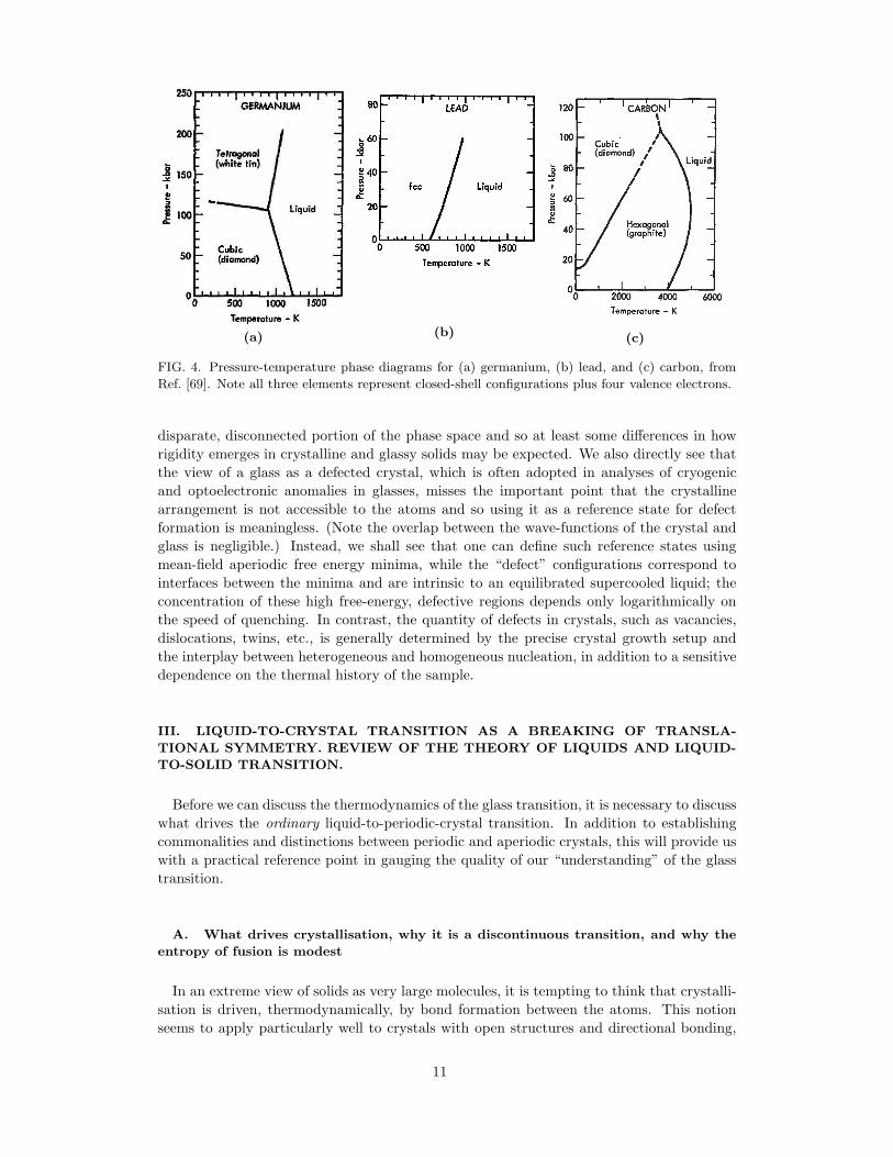
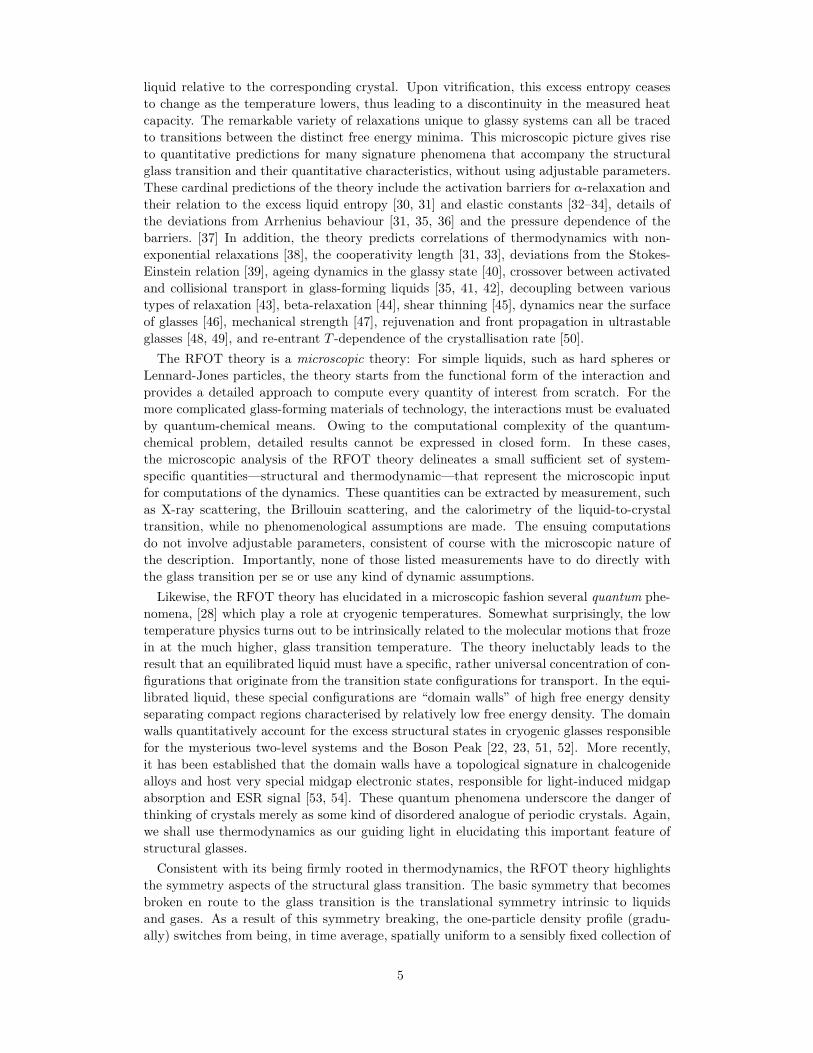
(a) (b) (c)

FIG. 4. Pressure-temperature phase diagrams for (a) germanium, (b) lead, and (c) carbon, from

Ref. [69]. Note all three elements represent closed-shell configurations plus four valence electrons.

disparate, disconnected portion of the phase space and so at least some differences in how

rigidity emerges in crystalline and glassy solids may be expected. We also directly see that

the view of a glass as a defected crystal, which is often adopted in analyses of cryogenic

and optoelectronic anomalies in glasses, misses the important point that the crystalline

arrangement is not accessible to the atoms and so using it as a reference state for defect

formation is meaningless. (Note the overlap between the wave-functions of the crystal and

glass is negligible.) Instead, we shall see that one can define such reference states using

mean-field aperiodic free energy minima, while the “defect” configurations correspond to

interfaces between the minima and are intrinsic to an equilibrated supercooled liquid; the

concentration of these high free-energy, defective regions depends only logarithmically on

the speed of quenching. In contrast, the quantity of defects in crystals, such as vacancies,

dislocations, twins, etc., is generally determined by the precise crystal growth setup and

the interplay between heterogeneous and homogeneous nucleation, in addition to a sensitive

dependence on the thermal history of the sample.

III. LIQUID-TO-CRYSTAL TRANSITION AS A BREAKING OF TRANSLA-

TIONAL SYMMETRY. REVIEW OF THE THEORY OF LIQUIDS AND LIQUID-

TO-SOLID TRANSITION.

Before we can discuss the thermodynamics of the glass transition, it is necessary to discuss

what drives the ordinary liquid-to-periodic-crystal transition. In addition to establishing

commonalities and distinctions between periodic and aperiodic crystals, this will provide us

with a practical reference point in gauging the quality of our “understanding” of the glass

transition.

A. What drives crystallisation, why it is a discontinuous transition, and why the

entropy of fusion is modest

In an extreme view of solids as very large molecules, it is tempting to think that crystalli-

sation is driven, thermodynamically, by bond formation between the atoms. This notion

seems to apply particularly well to crystals with open structures and directional bonding,

11

such as Si, Ge, and H2O. In the (low pressure) solids of these substances, atoms are less

coordinated than in the corresponding liquids above melting, as witnessed by a positive

volume change following crystallisation: ∆V > 0, see the phase diagram of germanium in

Fig. 4(a). One expects that at higher pressures, the bonding anisotropy becomes progres-

sively subdominant to the steric repulsion, leading to the more conventional reduction in

volume upon freezing, ∆V < 0, as is the case for lead or high-pressure germanium, see

Fig. 4. Yet there is generally no simple correlation between the pressure and the sign of

∆V , as is exemplified by the phase diagram of carbon shown in Fig. 4(c). Although all

three elements in Fig. 4 represent closed-shell configurations plus four valence electrons,

they show very different phase behaviours. Clearly, bonding changes play a significant role

in the liquid-to-crystal transition and exhibit remarkable variety even for seemingly similar

electronic configurations.

Yet, while partially correct, the notion of the bonding-driven crystallisation is potentially

misleading. The majority of enthalpy change due to bonding in the condensed phase occurs

already during the vapour-to-liquid transition, whose latent heat is typically an order of

magnitude greater than that for the liquid-to-crystal transition. This fact is reflected in the

venerable Trouton’s rule [56], by which the entropy of condensation at normal pressure is

numerically close to 101kB per particle, compared with the fusion entropy of about 100kBmentioned earlier. Indeed, the fusion enthalpy is comparable to the kinetic energy and thus

is much lower than the bond enthalpy, suggesting the crystal stability is of somewhat subtle

origin.

The relatively small entropy change upon freezing can be understood using the follow-

ing qualitative, mean-field argument [64, 70, 71]: Neglecting correlation between particles’

movements, the partition function for the liquid can be roughly estimated as

Zliquid ∼ 1

N !

(VfΛ3

)N

, (1)

where Λ ≡ (2π~2/mkBT )1/2 is the de Broglie thermal wavelength. The quantity Vf is

the total “free” volume, i.e., the total volume of the system minus the combined volume

of the molecules which we approximate here as relatively rigid, compact objects. The

combinatorial factor 1/N ! reflects that the particles are indistinguishable (Ref. [55], Chapter

41). The symmetry of the Hamiltonian with respect to particle identity is physically realised

by the particles exchanging locations: The defining feature of an equilibrium liquid/gas is

the uniform distribution of a particle’s density on any meaningful time scale. This is just a

technical way to say that the liquid assumes the shape of its container. In contrast, particles

comprising a solid are confined to “cages” with specific locations in space, which enables one

to actually label the particles, even if they are indistinguishable otherwise. To estimate the

partition function for the corresponding solid, let us use the Einstein approximation—which

also neglects particle-particle correlations. Here we simply multiply the partition functions

for individual particles each rattling within its own cage. The cage volume is the free volume

per particle: Vf/N , thus yielding:

Zsolid ∼ 1

NN

(VfΛ3

)N

(2)

The N ! factor is now absent because particles in a solid can be labelled (according to

which lattice sites they are nearest to) and thus may be regarded as distinguishable, as

just mentioned. Consequently, the excess entropy of the liquid relative to the corresponding

crystal is about kB ln(NN/N !) ≃ NkB, roughly consistent with observation. We thus

tentatively conclude that the entropy of fusion is relatively small because the translational

(or “mixing”) entropy in the uniform liquid only modestly exceeds the vibrational entropy

12

of particle motions within assigned cages in the corresponding solid; the interactions enter

the analysis through the free volume and cage shape and contribute toward system-specific

corrections to the simple result NkB. Note that the modest value of the translational

entropy in gases/liquids is a consequence of an interaction that is of statistical origin. This

interaction is present even if the particles do not interact in energetic terms: Because two

configurations in which two identical particles are interchanged are not distinct, the volume

statistically available to an individual particle is not the total free volume Vf , but only a

tiny portion of it, i.e., eVf/N or so, see Eq. (1).

But, in the first place, why should the liquid-to-crystal transition ordinarily be first order?

This is not an entirely trivial question. For instance, early computer simulations [72], which

employed small system-sizes, were ambiguous as to the discontinuous nature of the transition

for hard spheres; particles had to be confined to individual cells in space to minimise effects

of fluctuations, see discussion in Ref. [73]. An early constructive argument in favour of

a discontinuous nature of the liquid-to-solid transition is contained in a prescient paper

published by Bernal in 1937 [74], to which we shall return in due time. Of the most general

applicability is Landau’s symmetry-based argument [75, 76], whose publication also dates to

1937 and also significantly predates the aforementioned liquid simulations. The main tool

in the argument is what is now known as the Landau-Ginzburg functional [26, 55],

F =

∫d3r[κ(∇φ)2/2 + V (φ)]. (3)

We begin from the simplest non-trivial approximation for the bulk free energy term, viz.,

in terms of a 4th order polynomial:

V (φ) ≡ A

2φ2 +

B

3φ3 +

C

4φ4. (4)

In the Landau-Ginzburg approach one makes a non-obvious assumption that both the bulk

term and the (∇φ)-dependent term—which we have truncated at the second order—are

well-behaved, i.e., analytic.

To make analysis constructive, the terms in the expansion (4) must be traced to physical

interactions. Let us do this first for a familiar system, namely, the Ising spin model with

the energy function

H = −∑

i<j

Jijσiσj , σi = ±1. (5)

One can formally write down the Helmholtz free energy of the magnet as a sum of two

contributions, both of which are uniquely determined by the average magnetisation on

individual sites:

F (mi) = Fid(mi) + Fex(mi) (6)

where the “ideal gas” contribution:

Fid(mi) = kBT∑

i

(1 +mi

2ln

1 +mi

2+

1−mi

2ln

1−mi

2

), (7)

is the free energy of N non-interacting, free spins and is simply the sum over the entropies

of individual, standalone spins, times (−T ). This expression can be easily derived by noting

that the energy of a free spin is zero while the entropy of a spin with average magnetisation

〈σi〉 = mi (8)

is equal to the log-number of distinct configurations of a macroscopic number N of spins,

of which N(1 +mi)/2 point up and N(1−mi)/2 point down (divided by N and multiplied

13

by kB). Thus the entropy of a free spin with average magnetisation mi is simply the

Gibbs mixing entropy of two ideal gases with mole fractions (1 + mi)/2 and (1 − mi)/2,

per particle. Now, the excess term includes all other contributions to the free energy and

is difficult to write down except in a few cases [26, 77]. We will content ourselves with a

mean-field approximation, which becomes exact when each spin interacts infinitely weakly

with an infinite number of other spins. For the Ising magnet from Eq. (5), this would imply

Jij = J/N , so that the energy scales linearly with N , see Problem 2-2 of Goldenfeld [26].

Because each spin is in “contact” with (N − 1) spins, this situation formally corresponds

to an infinite dimensional space, the exact dimensionality depending on the type of lattice.

For a cubic lattice, the dimensionality would be (N − 1)/2. In the mean-field limit, the

correlations between spin flips can be ignored, since 〈σiσj〉 ≈ 〈σi〉 〈σj〉+O(1/N)N→∞→ mimj .

The entropy of such a collection of uncorrelated spins is equal to that of N free spins, and so

Fex is simply the average energy, since F = E−TS. Averaging energy (5) in the mean-field

limit 〈σiσj〉 = mimj readily yields:

Fex(mi) = −∑

i<j

Jijmimj (mean-field limit). (9)

Note that given the knowledge of the free energy as a function of mi’s, the couplings Jijcan be determined by varying the free energy with respect to the magnetisation on sites i

and j:

Jij = − ∂2Fex

∂mi∂mj. (10)

(∂2Fid/∂mi∂mj) = 0, of course.

From now on, assume for concreteness that all of the couplings are positive: Jij > 0. In

a translationally invariant system, Jij = J(ri − rj), the local magnetisation that minimises

the functional is spatially uniform: mi = m, and is an appropriate order parameter. In this

strictest, spatially-uniform limit of the mean-field approximation, the Helmholtz free energy

of the magnet reads, per spin:

F (m)/N = kBT

(1 +m

2ln

1 +m

2+

1−m

2ln

1−m

2

)− 1

2(ΣjJij) m

2. (11)

The bulk free energy (11) is the analog of the bulk free energy V (φ) from Eq. (4).

The free energy cost of deviations from the strictly uniform configuration in Eq. (11) can be

estimated by still using a mean-field approximation. The thermally-averaged interaction en-

ergy from Eq. (9) can be re-written as −(1/2)∑

imi

∑j Jijmj ≃ −(1/2)

∑imi

∑j Jij1 +

(rj − ri)∇ + (1/2)[(rj − ri)∇]2m(r)|r=ri , where we have truncated the Taylor expan-

sion of mj ≡ m(rj) around point ri at the 2nd order; this suffices to account for the

longest wavelength fluctuations relative to the average magnetisation. If, on the other

hand, we have an anti-ferromagnet, then an expansion around a finite wave-vector q = q0should be performed, not q = 0. Now, after summation in j, the 0th order term in

the expansion gives the 2nd term on the r.h.s. of Eq. (11), while the 1st order term

drops out by symmetry (ri − ri+j) = −(ri − ri−j) and the 2nd order term simplifies to

−(1/2)[∑

j Jij(rj − ri)2/(2 · 3)]∑imi∇2m(ri). In this expression, we switch from discrete

summation to volume integration and integrate by parts to obtain, per spin:

1

2

[1

6

(Σjr

2ijJij

)](∇m)2. (12)

This term represents the square-gradient term κ(∇φ)2/2 in the Landau-Ginzburg expansion

(3) for our ferromagnet. (The one-particle, entropic term from Eq. (6) does not contribute to

14

the square-gradient term.) The coefficient(Σjr

2ijJij

), which corresponds with the coefficient

κ in Eq. (3), follows a general pattern: Insofar as the interaction Jij possesses a finite range

l, the coefficient scales with l2 times an energy scale that characterises the interaction.

Now, returning to the bulk energy (11), the interaction term is second order in the order

parameter m and is proportional to the coupling constant J , in reflection of its two-body

origin. The entropic contribution also has a quadratic contribution, but of positive sign;

it stabilises the symmetric phase, m = 0, at high temperatures. The total coefficient at

the second order term reads as: A = −(∑

j Jij) + kBT and vanishes at the critical (Curie)

temperature Tc = (∑

j Jij)/kB leading to a ferromagnetic ordering below the Curie point,

whereby macroscopic regions acquire non-zero magnetisation, m = ±(−A/C)1/2 6= 0. (The

Curie point is lowered when non-meanfield effects are included in the treatment [26].) Note

that the entropic part of the free energy limits the possible value of magnetisation: |m| < 1—

and thus renders the functional stable. In the low order expansion (4), such stability is

guaranteed by the quartic term, whereby C > 0, however there is no hard constraint on the

magnitude of m. (This is reasonable so long as |m| is not too close to its maximum value of

1.) The spontaneous magnetisation m = ±(−A/C)1/2 below the critical point corresponds

to a non-zero (local) field which, in effect, breaks the time-reversal symmetry of the full

Hamiltonians E(σi) = E(−σi). Incidentally, because of the time-reversal symmetry,

the coefficient B at the cubic term in the functional is identically zero for the Ising model,

which is an exception rather than the rule, as we shall see shortly.

To build a free energy functional of the form (4) that is appropriate for particles—we first

specify that the order parameter reflect fluctuations of the density around its equilibrium

value ρeq(r), which we regard for now as coordinate-dependent, for the sake of generality:

δρ(r) ≡ ρ(r)− ρeq(r). (13)

Analogously to Eq. (6), we present the total Helmholtz free energy of the liquid (whether

uniform of not) as the sum of the “ideal gas” and interacting, or “excess” free energy

contributions [78, 79]:

F [ρ(r)] = Fid[ρ(r)] + Fex[ρ(r)], (14)

The “ideal gas” part is given by the expression

Fid[ρ(r)] = kBT

∫d3rρ(r)

[ln(ρ(r)Λ3

)− 1]. (15)

This equation is the Helmholtz free energy of an ideal gas whose concentration is not neces-

sarily spatially-uniform. We split space into elemental volumes Vi, each containing Ni gas

particles: Fid =∑

i F(i)id = −kBT lnZ

(i)id = kBTVi(Ni/Vi)[ln(Ni/Vi)− 1], each of the partial

free energies F(i)id corresponds to Eq. (1) with Vf = Vi. Switching to continuum integration

Vi → d3r and replacing Ni/Vi with its value ρ(r) yields Eq. (15). The ideal-gas free energy

(15) is the liquid analog of the entropic free energy Eq. (7). The only (and non-essential)

difference that it also has an energetic contribution due to the kinetic energy of individual

particles; this contribution obligingly renders the argument of the logarithm in Eq. (15)

dimensionless.

Note Eq. (14) is formally exact; it embodies the main idea of the classical density func-

tional theory (DFT). The DFT builds on the Hohenberg-Kohn-Mermin theorem [80, 81],

which states that there is a unique free energy functional F [ρ(r)] that is minimised by the

equilibrium density profile ρeq(r). As in the ferromagnet case, the interacting part Fex can

be computed in 3D only approximately. Appropriate approximations will be discussed in

due time. For now, let us formally expand the free energy (14) as a power series in terms

15

c q

c (

r)(2

)

r/d

(a)

qd

(2)

(b)

FIG. 5. We display two specific examples of the direct correlation function, corresponding to the

Percus-Yevick (dashed line) and Henderson-Grundke [83] (solid line) approximations for the hard

sphere liquid. Panels (a) and (b) show the function and its Fourier image respectively. Note the

significantly finer scale on the positive portion of the vertical axis in panel (a).

of δρ(r), up to the second order:

F [ρ(r)] = F [ρeq(r)] + kBT

∫d3r

[ln(ρeq(r)Λ

3)− c(1)(r)

]δρ(r) (16)

+kBT

2

∫d3r1d

3r2 δρ(r1)

[1

ρeq(r1)δ(r1 − r2)− c(2)(r1, r2)

]δρ(r2)

where, by definition,

c(1)(r) ≡ −β δFex

δρ(r). (17)

and c(2)(r1, r2) is the standard direct correlation function:

c(2)(r1, r2) ≡ −β δ2Fex[ρ(r)]

δρ(r1) δρ(r2)

∣∣∣∣ρ(r)=ρeq(r)

, (18)

c.f. Eq. (10). Note that the direct correlation function is translationally invariant and

isotropic for a bulk uniform liquid

ρeq(r) = ρliq

c(1)(r) = c(1)liq (19)

c(2)(r1, r2) = c(2)(|r1 − r2|),

but this assumption is not strictly correct in liquids that are not uniform—as would be the

case in an otherwise homogeneous fluid near a wall or liquid-vapour interface [79] and, of

course, in crystals [82].

As in the ferromagnet case, the second order term in Eq. (16) accounts for the two-body

contributions to the free energy. Appropriately, it can be seen from Eq. (16) that in the

16

weak-interaction limit [78]:

c(2)(r1, r2) → −βv(r1, r2), as ρ→ 0, (20)

and so in this limit, the direct correlation function has the same range as the pairwise

interaction v(r1, r2). Even near critical points, where the full density-density correlation

function becomes so long-ranged that the compressibility diverges, the direct correlation

function remains integrable (see Eq. (69) and (70) below). The direct correlation function

c(2)(r1, r2) includes all interactions between these two particles, including those induced by

the rest of the particles. For instance, c(2)(r) for the hard sphere liquid has a positive—i.e.,

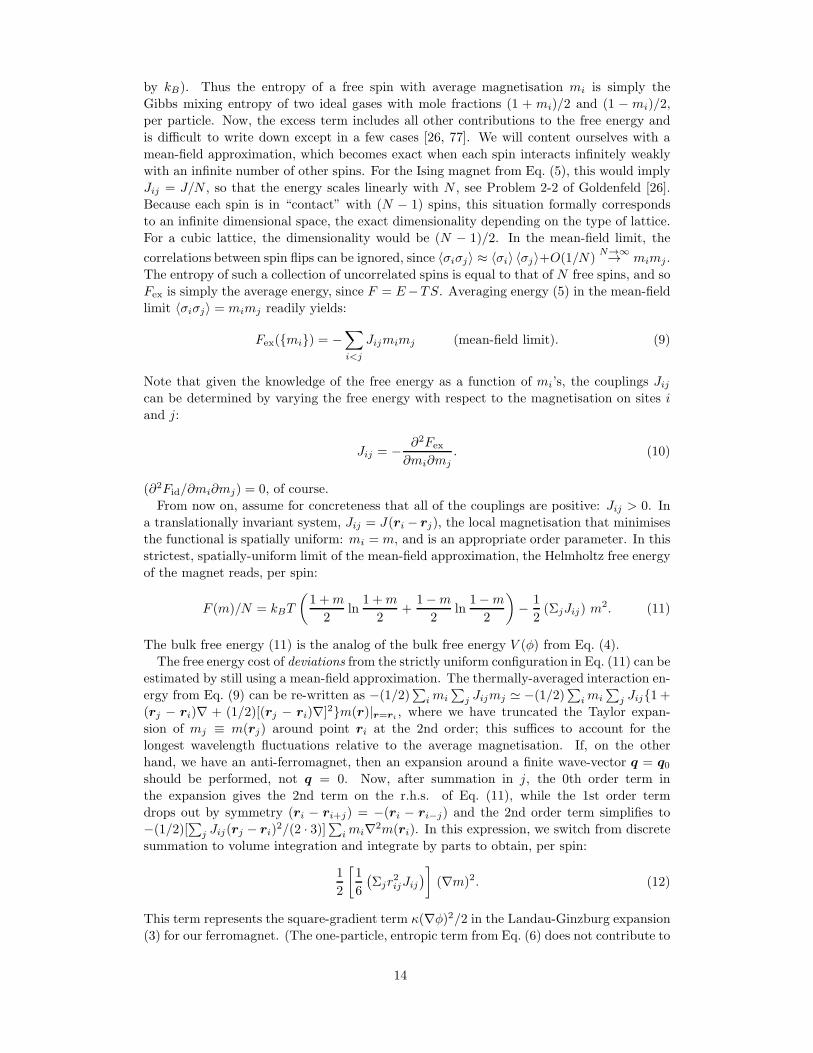
“attractive” by Eq. (20)—tail around r = d, see Fig. 5(a). Two neighbouring particles

are effectively pushed together by being repelled from the surrounding particles. (This is

analogous to the so called “depletion interaction” that can be induced between molecules

by adding polymer to the solution [84].) At short separations, r < d, the direct correlation

function has a rather different meaning. Namely, it scales (with the negative sign) with the

bulk modulus of the liquid. This notion will be made precise in a short while. For now, it is

instructive to compare the free energy cost of quadratic fluctuations in Eq. (16) to the free

energy cost of a weak deformation of an elastic continuum [85]:

F =

∫∫d3r1d

3r2D(r1 − r2)

[(K

2− µ

3

)ujj(r1)ull(r2) + µu′ij(r1)u

′ij(r2)

](21)

where the deformation tensor uij is defined in the standard fashion:

uij = (1/2) (∂ui/∂xj + ∂uj/∂xi) (22)

and u′ij stands for its traceless portion u′ij ≡ uij − 13δijull that corresponds to pure shear.

The vector u gives a particle’s displacement relative to its equilibrium position, while its

divergence uii yields the relative volume change of a compact region encompassing a specific

group of atoms, due to uniform contraction or dilation. Eq. (21) corresponds to a non-local

form of the elasticity theory [86–88], which is reduced to the classic, ultra-local approxi-

mation [85] by taking the limit D(r) → δ(r). In this continuum limit, the coefficient K

corresponds with the macroscopic bulk modulus:

K ≡ −V(∂p

∂V

)

T

, (23)

while µ becomes the standard shear modulus. This is where we can make connection with

the functional in Eq. (16), since the δρ’s in that equation also scale with local volume

changes. For a region containing an appreciable number of particles, δρ/ρ = −uii. Despite

this relation, we note that there is generally no one-to-one correspondence between the

deformation tensor uij and the local density variation δρ because the former is a quantity

coarse-grained over a mesoscopic region, while the latter is defined on an arbitrarily small

length scale and can change arbitrarily rapidly in space. For instance, for a stationary

particle at the origin, ρ(r) = δ(r). Now, to connect the functionals (16) and (21), we

first set µ = 0 as is appropriate for uniform liquids. Because only long-wavelength density

variations can be compared between the two functionals, we can adopt the continuum limit

of the elasticity: F = (1/2)∫d3rKu2jj(r), yielding Ku

2jj(r)/2 for the free energy density at

location r. By Eq. (16), the same quantity is given by (kBT/2)δρ2(r)

∫d3r[1/ρeq− c(2)(r)],

where we used that the direct correlation function decays much faster than the lengthscale

for density variations. For such slow variations, δρ/ρ = −uii, and we obtain:

− ρliq

∫d3rc(2)(r) =

K

kBTρliq

− 1, (24)

17

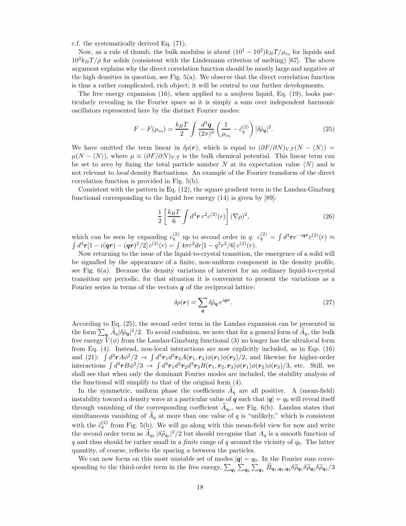
c.f. the systematically derived Eq. (71).

Now, as a rule of thumb, the bulk modulus is about (101 − 102)kBT/ρliq for liquids and

102kBT/ρ for solids (consistent with the Lindemann criterion of melting) [67]. The above

argument explains why the direct correlation function should be mostly large and negative at

the high densities in question, see Fig. 5(a). We observe that the direct correlation function

is thus a rather complicated, rich object; it will be central to our further developments.

The free energy expansion (16), when applied to a uniform liquid, Eq. (19), looks par-

ticularly revealing in the Fourier space as it is simply a sum over independent harmonic

oscillators represented here by the distinct Fourier modes:

F − F (ρliq) =kBT

2

∫d3q

(2π)3

(1

ρliq

− c(2)q

)|δρq|2. (25)

We have omitted the term linear in δρ(r), which is equal to (∂F/∂N)V,T (N − 〈N〉) =

µ(N − 〈N〉), where µ ≡ (∂F/∂N)V,T is the bulk chemical potential. This linear term can

be set to zero by fixing the total particle number N at its expectation value 〈N〉 and is

not relevant to local density fluctuations. An example of the Fourier transform of the direct

correlation function is provided in Fig. 5(b).

Consistent with the pattern in Eq. (12), the square gradient term in the Landau-Ginzburg

functional corresponding to the liquid free energy (14) is given by [89]:

1

2

[kBT

6

∫d3r r2c(2)(r)

](∇ρ)2, (26)

which can be seen by expanding c(2)q up to second order in q: c

(2)q =

∫d3re−iqrc(2)(r) ≈∫

d3r[1− i(qr)− (qr)2/2] c(2)(r) =∫4πr2dr[1 − q2r2/6] c(2)(r).

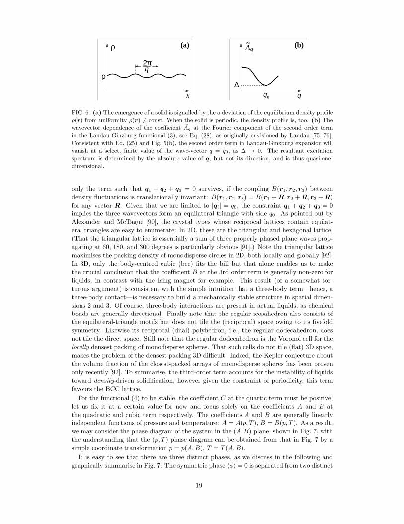
Now returning to the issue of the liquid-to-crystal transition, the emergence of a solid will

be signalled by the appearance of a finite, non-uniform component in the density profile,

see Fig. 6(a). Because the density variations of interest for an ordinary liquid-to-crystal

transition are periodic, for that situation it is convenient to present the variations as a

Fourier series in terms of the vectors q of the reciprocal lattice:

δρ(r) =∑

q

δρq eiqr. (27)

According to Eq. (25), the second order term in the Landau expansion can be presented in

the form∑

q Aq|δρq|2/2. To avoid confusion, we note that for a general form of Aq, the bulk

free energy V (φ) from the Landau-Ginzburg functional (3) no longer has the ultralocal form

from Eq. (4). Instead, non-local interactions are now explicitly included, as in Eqs. (16)

and (21):∫d3rAφ2/2 →

∫d3r1d

3r2A(r1, r2)φ(r1)φ(r2)/2, and likewise for higher-order

interactions∫d3rBφ3/3 →

∫d3r1d

3r2d3r3B(r1, r2, r3)φ(r1)φ(r2)φ(r3)/3, etc. Still, we

shall see that when only the dominant Fourier modes are included, the stability analysis of

the functional will simplify to that of the original form (4).

In the symmetric, uniform phase the coefficients Aq are all positive. A (mean-field)

instability toward a density wave at a particular value of q such that |q| = q0 will reveal itself

through vanishing of the corresponding coefficient Aq0 , see Fig. 6(b). Landau states that

simultaneous vanishing of Aq at more than one value of q is “unlikely,” which is consistent

with the c(2)q from Fig. 5(b). We will go along with this mean-field view for now and write

the second order term as Aq0 |δρq0 |2/2 but should recognise that Aq is a smooth function of

q and thus should be rather small in a finite range of q around the vicinity of q0. The latter

quantity, of course, reflects the spacing a between the particles.

We can now focus on this most unstable set of modes |q| = q0. In the Fourier sum corre-

sponding to the third-order term in the free energy,∑

q1

∑q2

∑q3Bq1,q2,q3

δρq1δρq2

δρq3/3

18

(b)

ρ

x

q2π

ρ

∆q0 q

Aq~(a)

FIG. 6. (a) The emergence of a solid is signalled by the a deviation of the equilibrium density profile

ρ(r) from uniformity ρ(r) 6= const. When the solid is periodic, the density profile is, too. (b) The

wavevector dependence of the coefficient Aq at the Fourier component of the second order term

in the Landau-Ginzburg functional (3), see Eq. (28), as originally envisioned by Landau [75, 76].

Consistent with Eq. (25) and Fig. 5(b), the second order term in Landau-Ginzburg expansion will

vanish at a select, finite value of the wave-vector q = q0, as ∆ → 0. The resultant excitation

spectrum is determined by the absolute value of q, but not its direction, and is thus quasi-one-

dimensional.

only the term such that q1 + q2 + q3 = 0 survives, if the coupling B(r1, r2, r3) between

density fluctuations is translationally invariant: B(r1, r2, r3) = B(r1 +R, r2 +R, r3 +R)

for any vector R. Given that we are limited to |qi| = q0, the constraint q1 + q2 + q3 = 0

implies the three wavevectors form an equilateral triangle with side q0. As pointed out by

Alexander and McTague [90], the crystal types whose reciprocal lattices contain equilat-

eral triangles are easy to enumerate: In 2D, these are the triangular and hexagonal lattice.

(That the triangular lattice is essentially a sum of three properly phased plane waves prop-

agating at 60, 180, and 300 degrees is particularly obvious [91].) Note the triangular lattice

maximises the packing density of monodisperse circles in 2D, both locally and globally [92].

In 3D, only the body-centred cubic (bcc) fits the bill but that alone enables us to make

the crucial conclusion that the coefficient B at the 3rd order term is generally non-zero for

liquids, in contrast with the Ising magnet for example. This result (of a somewhat tor-

turous argument) is consistent with the simple intuition that a three-body term—hence, a

three-body contact—is necessary to build a mechanically stable structure in spatial dimen-

sions 2 and 3. Of course, three-body interactions are present in actual liquids, as chemical

bonds are generally directional. Finally note that the regular icosahedron also consists of

the equilateral-triangle motifs but does not tile the (reciprocal) space owing to its fivefold

symmetry. Likewise its reciprocal (dual) polyhedron, i.e., the regular dodecahedron, does

not tile the direct space. Still note that the regular dodecahedron is the Voronoi cell for the

locally densest packing of monodisperse spheres. That such cells do not tile (flat) 3D space,

makes the problem of the densest packing 3D difficult. Indeed, the Kepler conjecture about

the volume fraction of the closest-packed arrays of monodisperse spheres has been proven

only recently [92]. To summarise, the third-order term accounts for the instability of liquids

toward density-driven solidification, however given the constraint of periodicity, this term

favours the BCC lattice.

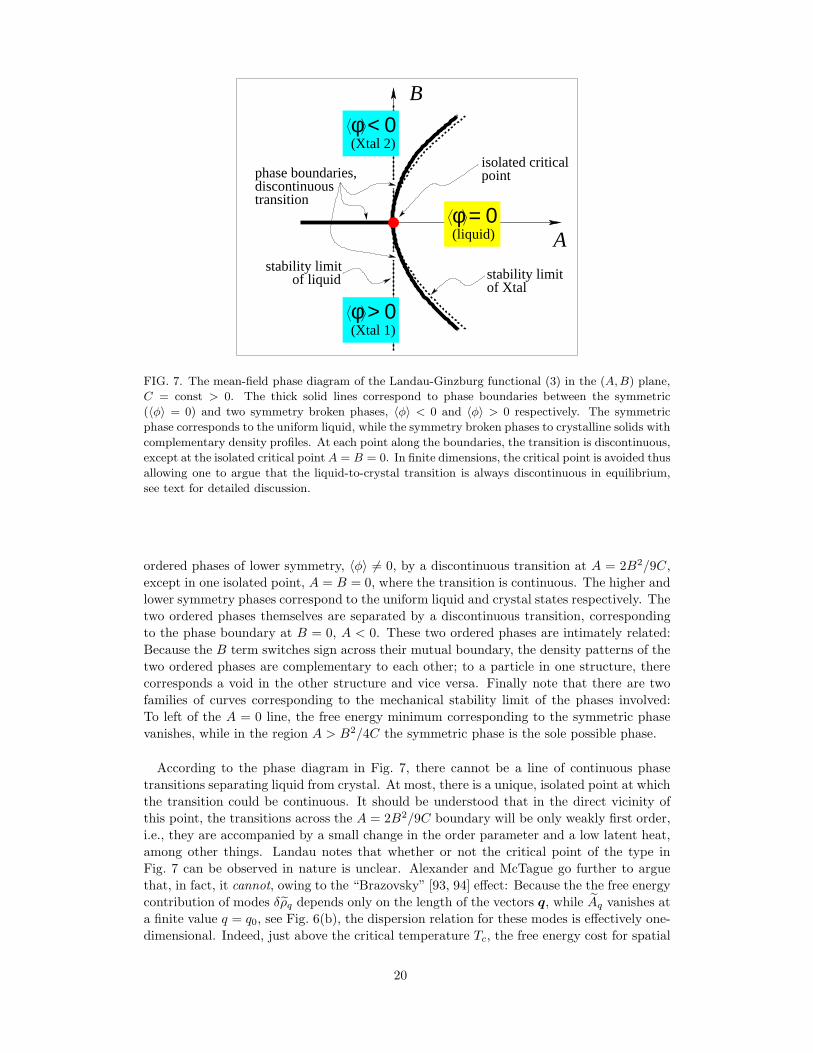
For the functional (4) to be stable, the coefficient C at the quartic term must be positive;

let us fix it at a certain value for now and focus solely on the coefficients A and B at

the quadratic and cubic term respectively. The coefficients A and B are generally linearly

independent functions of pressure and temperature: A = A(p, T ), B = B(p, T ). As a result,

we may consider the phase diagram of the system in the (A,B) plane, shown in Fig. 7, with

the understanding that the (p, T ) phase diagram can be obtained from that in Fig. 7 by a

simple coordinate transformation p = p(A,B), T = T (A,B).

It is easy to see that there are three distinct phases, as we discuss in the following and

graphically summarise in Fig. 7: The symmetric phase 〈φ〉 = 0 is separated from two distinct

19

B

isolated criticalpoint

stability limitof Xtal

of liquidstability limit

phase boundaries,discontinuoustransition

A

(Xtal 2)

φ = 0(liquid)

φ > 0(Xtal 1)

φ < 0

FIG. 7. The mean-field phase diagram of the Landau-Ginzburg functional (3) in the (A,B) plane,

C = const > 0. The thick solid lines correspond to phase boundaries between the symmetric

(〈φ〉 = 0) and two symmetry broken phases, 〈φ〉 < 0 and 〈φ〉 > 0 respectively. The symmetric

phase corresponds to the uniform liquid, while the symmetry broken phases to crystalline solids with

complementary density profiles. At each point along the boundaries, the transition is discontinuous,

except at the isolated critical pointA = B = 0. In finite dimensions, the critical point is avoided thus

allowing one to argue that the liquid-to-crystal transition is always discontinuous in equilibrium,

see text for detailed discussion.

ordered phases of lower symmetry, 〈φ〉 6= 0, by a discontinuous transition at A = 2B2/9C,

except in one isolated point, A = B = 0, where the transition is continuous. The higher and

lower symmetry phases correspond to the uniform liquid and crystal states respectively. The

two ordered phases themselves are separated by a discontinuous transition, corresponding

to the phase boundary at B = 0, A < 0. These two ordered phases are intimately related:

Because the B term switches sign across their mutual boundary, the density patterns of the

two ordered phases are complementary to each other; to a particle in one structure, there

corresponds a void in the other structure and vice versa. Finally note that there are two

families of curves corresponding to the mechanical stability limit of the phases involved:

To left of the A = 0 line, the free energy minimum corresponding to the symmetric phase

vanishes, while in the region A > B2/4C the symmetric phase is the sole possible phase.

According to the phase diagram in Fig. 7, there cannot be a line of continuous phase

transitions separating liquid from crystal. At most, there is a unique, isolated point at which

the transition could be continuous. It should be understood that in the direct vicinity of

this point, the transitions across the A = 2B2/9C boundary will be only weakly first order,

i.e., they are accompanied by a small change in the order parameter and a low latent heat,

among other things. Landau notes that whether or not the critical point of the type in

Fig. 7 can be observed in nature is unclear. Alexander and McTague go further to argue

that, in fact, it cannot, owing to the “Brazovsky” [93, 94] effect: Because the the free energy

contribution of modes δρq depends only on the length of the vectors q, while Aq vanishes at

a finite value q = q0, see Fig. 6(b), the dispersion relation for these modes is effectively one-

dimensional. Indeed, just above the critical temperature Tc, the free energy cost for spatial

20

density variations reads (in the quadratic approximation and in D spatial dimensions):

F − Funi =1

2

∫dDq

(2π)DAq|δρq|2 ∝

∫qD−1dq

[∆+ (q − q0)

2]|δρq|2, (28)

c.f. Eqs.(25) and Fig. (5)(b). Clearly, the r.h.s. integral above is one-dimensional. On the

other hand, the Landau-Ginzburg bulk energy describes the breaking of a discrete symmetry,

φ ↔ −φ, as B → 0. The Curie point of an Ising ferromagnet is a good example of such

a discrete symmetry breaking. Critical points of this type are generally suppressed by

fluctuations in one-dimensional systems at finite temperatures [55]. (This is true unless

the interactions are very long range, 1/r2 or slower [95, 96]; note excitations in elastic 3D

solids interact at best according to 1/r3 [85], see also below.) In the present context, these

criticality-destroying fluctuations are motions of domain walls separating the two symmetry

broken phases corresponding to B > 0 and B < 0 and are indeed quasi-one dimensional

for interfaces with sufficiently low curvature. The Brazovsky effect implies that not only

is the phase boundary between the symmetric and broken-symmetry phases moved down

toward lower values of A owing to fluctuations—as it generally would—it also dictates that

the continuous transition at B = 0 will be pushed all the way down to T = 0. Thus, the

liquid-to-crystal transition is always first order in equilibrium. (Conversely, one may be able

to sample some of this criticality by using rapid quenches, to be discussed in due time.) We

also note that to understand what actually happens at B = 0, A < 0, i.e., which polymorph

will be ultimately chosen by the system, generally requires knowledge of higher order terms

in the functional (4).

The erasure of the critical point is not the only non-meanfield effect we should be mindful

of. Recall that the coefficient Aq is small in a finite vicinity of the vector q. This means that

lattice types other than BCC, such as FCC, can become stable [97]. It is these structures

in which the system could settle when the critical point at A = B = 0 is avoided. Indeed,

elemental solids display a variety of structures, with bcc being far from prevalent. Still,

Alexander and McTague have argued that even if the BCC structure is not the most stable,

it is likely most kinetically-accessible, especially near weakly discontinuous liquid-to-solid

transitions, consistent with experiment [90].

The simplest possible approximation (4), in which one truncates the Landau-Ginzburg

expansion at the fourth-order term, apparently covers the worst-case scenario in the sense

that the presence of negative terms of order higher than three will only act to further suppress

a continuous liquid-to-crystal transition. Indeed, suppose the coefficient C at the fourth-

order term in Eq. (4) is negative, which dictates that we now expand the free energy up to

the sixth order or higher. A negative fourth-order term stabilises a broken-symmetry phase,

φ 6= 0, even if the third-order term is strictly zero. Important examples of crystal-lattice

types for which the fourth or higher order terms must be non-zero include the graphite,

diamond, and simple-cubic lattices. For instance, to stabilise the graphite lattice, not only

should the bond-angle be fixed at sixty degrees, for which a third-order term alone would

suffice. In addition, the three bonds emanating from an individual particle must be stabilised

in the planar arrangement. In the case of the diamond lattice, it is likely that the fifth-

order term is non-zero, too: While a fourth-order term alone could stabilise local pyramidal

configuration in which the bond-angles are at the requisite value of 109.4, the resulting

energy function could also favour stacked double-layers giving rise to a rhombohedral lattice,

in addition to the diamond structure. (The latter stacked structure is exemplified by arsenic,

however the angle is intermediate between 109.4 and 90.) Likewise, a structure with

enforced 90 bond-angles could, in principle, be simple-cubic but such a structure is often

unstable toward tetragonal distortion. Interestingly, the only elemental solid that has the

simple-cubic lattice structure at normal pressure is polonium. (Arsenic, phosphorus, and, of

all things, calcium can be made simple-cubic by applying pressure [98, 99].) Consistent with

21

these notions, we know for a fact that interactions in actual crystals are truly many-body and

are even affected by (electronic) relativistic effects [100]. Note the diamond, graphite, and

simple-cubic lattices are some of the most open structures encountered in actual crystals.

(Low density structure with nanovoids can be readily made [101] but are not uniformly

open.)

The following picture emerges from the above discussion: The presence of a significant,

fourth (or higher) order stabilising contribution to the free energy of the liquid leads to

the formation of open structures with very directional bonding and thus reduces the effects

of steric repulsion on the liquid-to-solid transition. At the same time the discontinuity of

the liquid-to-crystal transition is relatively large, see discussion at the end of this Section.

Liquids that freeze into the diamond lattice and expand alongside illustrate this situation

particularly well. Conversely, if such high order terms in the free energy expansion are

weak, excluded-volume effects become important that are accounted for by the third-order

term. The smaller the third order term, the milder the discontinuity of the liquid-to-solid

transition (if the higher-order terms are non-negative!). Still, the third-order terms cannot

completely disappear in equilibrium because of the steric effects. On the other hand, quasi-

one dimensional fluctuations would destroy the critical point, even if the third-order terms

were very small. We thus conclude that those quasi-one dimensional fluctuations are also of

steric origin. We reiterate that despite their importance, the steric effects are not the only

player. It is essential to remember that the liquid is equilibrated at a finite temperature and,

thus, is not jammed; the particles ultimately are allowed to vibrate and exchange places.

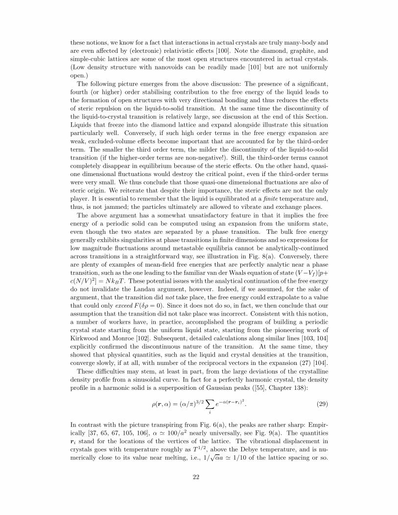
The above argument has a somewhat unsatisfactory feature in that it implies the free

energy of a periodic solid can be computed using an expansion from the uniform state,

even though the two states are separated by a phase transition. The bulk free energy

generally exhibits singularities at phase transitions in finite dimensions and so expressions for

low magnitude fluctuations around metastable equilibria cannot be analytically-continued

across transitions in a straightforward way, see illustration in Fig. 8(a). Conversely, there

are plenty of examples of mean-field free energies that are perfectly analytic near a phase

transition, such as the one leading to the familiar van der Waals equation of state (V −Vf )[p+c(N/V )2] = NkBT . These potential issues with the analytical continuation of the free energy

do not invalidate the Landau argument, however. Indeed, if we assumed, for the sake of

argument, that the transition did not take place, the free energy could extrapolate to a value

that could only exceed F (δρ = 0). Since it does not do so, in fact, we then conclude that our

assumption that the transition did not take place was incorrect. Consistent with this notion,

a number of workers have, in practice, accomplished the program of building a periodic

crystal state starting from the uniform liquid state, starting from the pioneering work of

Kirkwood and Monroe [102]. Subsequent, detailed calculations along similar lines [103, 104]

explicitly confirmed the discontinuous nature of the transition. At the same time, they

showed that physical quantities, such as the liquid and crystal densities at the transition,

converge slowly, if at all, with number of the reciprocal vectors in the expansion (27) [104].

These difficulties may stem, at least in part, from the large deviations of the crystalline

density profile from a sinusoidal curve. In fact for a perfectly harmonic crystal, the density

profile in a harmonic solid is a superposition of Gaussian peaks ([55], Chapter 138):

ρ(r, α) = (α/π)3/2∑

i

e−α(r−ri)2

. (29)

In contrast with the picture transpiring from Fig. 6(a), the peaks are rather sharp: Empir-

ically [37, 65, 67, 105, 106], α ≃ 100/a2 nearly universally, see Fig. 9(a). The quantities

ri stand for the locations of the vertices of the lattice. The vibrational displacement in

crystals goes with temperature roughly as T 1/2, above the Debye temperature, and is nu-

merically close to its value near melting, i.e., 1/√αa ≃ 1/10 of the lattice spacing or so.

22

(b)

φ

F

actual free energy

analyticalcontinuation

F

g m

(a)

FIG. 8. (a) This sketch illustrates that analytical continuation of the free energy between distinct

phases is generally ill-defined. (b) Thick solid line: The Helmholtz free energy F of a spatially

uniform ferromagnet below the Curie point, as a function of the average magnetisation m ≡M/N

(M is the total magnetisation). The region separating the two minima is non-concave; one cannot

use the Legendre transform to compute the Gibbs free energy G: G = F −Mh, h = (∂F/∂M)T .

In equilibrium, the system phase-separates, and so the actual, equilibrium Helmholtz free energy

between the two minima in F is given by the thick dashed line. The latter line is entirely analogous

to the red line in Fig. 1(b).

The latter quotient should be nearly universal, as was argued by Lindemann more than a

century ago. It is by no means intuitively obvious that the vibrational displacement near

melting, which is often called the Lindemann length, should as small as one-tenths. Linde-

mann himself [107] thought that this displacement should be about a half of the particle

spacing, which would be more consistent with the mild density variation in Fig. 6(a) than

with the sharp peaks in Fig. 9(a). Lindemann’s (correct) logic was that the melting was

caused by intense collisions between the atoms. Still, both experiment and theory indicate

the dramatic anharmonicities that eventually lead to crystal’s disintegration should become

important already at α ≃ 100/a2. In Subsection IVA, we shall see that for rigid particles,

the quantity αa2 is essentially given by the number of particles in the first coordination shell

(up to a logarithmic correction and a constant factor), which scales as the dimensionality

of space squared, see Eq. (83).

It is straightforward to obtain an explicit expression for α—which is the “spring constant”

of an effective Einstein oscillator—given a specific form of the phonon spectrum. For in-

stance, assuming isotropic elasticity with the isothermal bulk modulus K and shear modulus

µ and a Debye phonon spectrum with an ultraviolet cutoff at |k| = π/a, one obtains [42]:

α−1 ≡ 1

a

kBT

3πµ

6K + 11µ

3K + 4µ. (30)

It is particularly straightforward to discuss the driving force for the crystallisation of

hard spheres, which do not form actual bonds and for which the enthalpy change during the

transition:

∆Hm = ∆Em + pm∆Vm (31)

is entirely due to the work needed to compress the liquid: ∆Vm < 0, at constant temper-

ature. The stability of the hard sphere crystal, relative to the corresponding liquid (gas),

stems from the notion that the densest packing of monodisperse spheres in 3D is a periodic

crystal—face-centred cubic (FCC) or hexagonal close-packed HCP—which now appears to

be rigorously proven [92]. This notion has resisted systematic effort since time of Kepler

and is non-trivial because the most compact Voronoi cell of a particle surrounded by twelve

neighbours—the highest number allowed in 3D—is the regular dodecahedron. The latter

23

has a five-fold symmetry and thus does not tile space. As follows from the proof of the

Kepler conjecture, one can say that thermodynamically, the transition is density-driven or,

equivalently, sterically-driven. Already the original Landau argument from 1937, which ne-

glects fluctuations, suffices to show that the transition in hard spheres is first order: All

points on the liquid-crystal phase boundary in the (p, T ) plane are equivalent because the

p/T ratio in hard spheres is determined by the density exclusively. Thus, it is impossible to

have an isolated critical point on that phase boundary.

To give a partial summary, the liquid-to-crystal transition is a discontinuous phase tran-

sition resulting in a breaking of translational symmetry, upon which individual particles

occupy specific cells in space as opposed the whole space. The fusion entropy is essentially

the difference between the entropy of translational motion in the uniform liquid and the vi-

brational entropy in the crystal. Consistent with this, the fusion entropy in open structures

often exceeds that for crystallisation of well-packed structures, as we shall see explicitly in

Subsection III C. For rigid particles, crystallisation is driven by steric repulsion alone. The

liquid-to-crystal transition breaks a continuous symmetry. Breaking such a symmetry re-

sults in the emergence of Goldstone modes [26] below the transition, which are represented

in crystals by the phonons [91]. To put this in perspective, the symmetry of the Hamilto-

nian to simultaneous flips of all spins σi ↔ −σi, which is broken during ferromagnetic

ordering, is a discrete symmetry, see Fig. 8.

B. Emergence of the Molecular Field

A methodological advantage of studying a monodisperse, hard-sphere liquid is that one

can gain qualitative insight into its crystallisation while being able to test the corresponding

approximations against simulations. Such tested approximations will come in handy when

studying the emergence of rigidity in aperiodic systems, since monodisperse hard spheres

crystallise too readily thus preventing one from achieving meaningfully deep quenches in a

direct simulation.

Most of the quantitative theories of liquid-to-solid transition can be traced back to the

very old idea of the “molecular field,” which was originally conceived in the context of the

vapour-to-liquid transition by van der Waals [108] and in the context of ferromagnetism

by Curie and Weiss [10, 109]. We have already benefited from thinking about the latter

system; let us use it again to illustrate the concept of the molecular field. For a collection of

Ising spins, Eq. (5), spin i is subject to an instantaneous field∑

j Jijσj . If we, in the mean-

field fashion, ignore correlations in spin flips: 〈σiσj〉 ≈ 〈σi〉 〈σj〉, the (thermally-averaged)

value of the molecular field hmoli is simply given by the expression: hmol

i =∑

j Jijmj. We

observe that when a ferromagnet spontaneously polarises, so that mi > 0 or mi < 0, this

effective field becomes non-zero thus breaking the time-reversal symmetry σi ↔ −σi of

the Hamiltonian H = −∑i<j Jijσiσj .

A systematic way to implement the concept of the effective field is to employ an additional

ensemble. The Helmholtz free energy in Eq. (6) is the appropriate thermodynamic potential

at fixed magnetisation and is analogous to the canonical construction for particulate systems,

in which one fixes the volume of the system. Alternatively, one may use the ensemble in

which the magnetisation is allowed to fluctuate while the magnetic field is fixed. In gases,

this is analogous to allow for volume changes at fixed particle number, while subjecting

the gas to external pressure (the isobaric ensemble); the corresponding thermodynamic

potential is the Gibbs free energy G = F + pV . Alternatively, one may allow the particle

number to change at fixed V , while imposing a specific value of the chemical potential (the

grand-canonical ensemble); the corresponding free energy is Ω = F − µN = −pV [55, 110].

To evaluate the Gibbs free energy for the magnet, let us formally write down the partition

24

function for the energy function from Eq. (5) with an added term −∑i hiσi:

Z(hi) =∑

σi=±1exp[−β(H−

∑

i

hiσi)]. (32)

Clearly, the average magnetisation mi ≡ 〈σi〉 can be computed according to:

mi = −(∂G(hi)∂hi

)

T

, (33)

where G(hi) ≡ −kBT lnZ(hi) is a function of the fields hi. It is easy to convince

oneself (without actually computing Z) that one can write out this (Gibbs) free energy as

G = −∑imihi + E − TS, where E ≡ 〈H〉 is the energy while the quantity S is equal to

−(∂G/∂T )hi and thus must be identified with the entropy. Consequently, the function

F = G+∑

imihi = E−TS must be identified with the Helmholtz free energy, which we have

seen can be expressed exclusively as a function of local magnetisations mi: F = F (mi).On the other hand, dF = dG+ d(

∑imihi) = −SdT +

∑i hidmi, and so one has for spin i:

hi =

(∂F (mi)∂mi

)

T

. (34)

The meaning of Eq. (33) is that one solves for hi such that satisfy the equation for a

specified set of magnetisations mi’s. Likewise, one solves for mi such that satisfy Eq. (34)

for a chosen set of on-site fields hi. It would appear that the two descriptions in Eq. (33) and

(34) are equivalent, so that either one can be used. In fact, the Gibbs ensemble is often more

computationally convenient and thus is used more frequently. However, the two descriptions,

which are related by a Legendre transform: F = G+∑

imihi, are only equivalent if both F

orG are concave or convex [111], which is certainly not the case for the ferromagnet below its

Curie point, see Fig. 8. This figure demonstrates that while to a given value of magnetisation

m there corresponds a unique value of the field h = ∂F/∂m, the converse is not generally

true: Up to three distinct solutions exist for equation h = ∂F/∂m when the F (m) curve has

a convex-up portion. Furthermore, for h = 0, the two stable solutions for the magnetisation

are exactly degenerate in free energy, thus making the choice between distinct solutions of

Eqs. (34) particularly ambiguous. Furthermore, if one enforces summation over spin states

in the partition function from Eq. (32), at hi = 0, one will recover mi = 0 even below

the Curie point, thus missing the transition. This apparent—but incorrectly determined—

equilibrium value of mi = 0 is an unstable solution of the free energy functional! This

problematic situation would not arise in the Helmholtz ensemble, which clearly shows the

two polarised states as minima of the free energy. These notions indicate that the Helmholtz

ensemble is more basic than the Gibbs ensemble. In much the same way, the microcanonical

ensemble is more basic than the canonical ensemble in the context of Fig. 1(a); the isochoric

ensemble is more basic than the isobaric ensemble in Fig. 1(b).

For an individual spin, however, the h ↔ m correspondence is one-to-one and we may

safely choose to work with either the magnetisation mi or the corresponding “molecular

field” hmoli :

hmoli =

∂Fid

∂mi⇒ hmol

i = kBT tanh−1(mi) ⇔ mi = tanhβhmoli (35)

For the field-less energy function in Eq. (5), hi = 0, and so the equilibrium configuration

of mi simply optimises the free energy F :

∂F

∂mi= 0, (36)

25

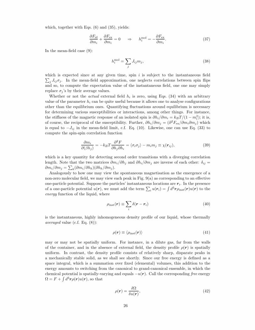
which, together with Eqs. (6) and (35), yields:

∂Fid

∂mi+∂Fex

∂mi= 0 ⇒ hmol

i = −∂Fex

∂mi. (37)

In the mean-field case (9):

hmoli =

∑

j

Jijmj , (38)

which is expected since at any given time, spin i is subject to the instantaneous field∑j Jijσj . In the mean-field approximation, one neglects correlations between spin flips

and so, to compute the expectation value of the instantaneous field, one one may simply

replace σj ’s by their average values.

Whether or not the actual external field hi is zero, using Eqs. (34) with an arbitrary

value of the parameter hi can be quite useful because it allows one to analyse configurations

other than the equilibrium ones. Quantifying fluctuations around equilibrium is necessary

for determining various susceptibilities or interactions, among other things. For instance,

the stiffness of the magnetic response of an isolated spin is ∂hi/∂mi = kBT/(1−m2i ); it is,

of course, the reciprocal of the susceptibility. Further, ∂hi/∂mj = (∂2Fex/∂mi∂mj) which

is equal to −Jij in the mean-field limit, c.f. Eq. (10). Likewise, one can use Eq. (33) to

compute the spin-spin correlation function

∂mi

∂(βhj)= −kBT

∂2F

∂hj∂hi= 〈σiσj〉 −mimj ≡ χ(rij), (39)

which is a key quantity for detecting second order transitions with a diverging correlation

length. Note that the two matrices ∂mi/∂hj and ∂hi/∂mj are inverse of each other: δij =

∂mi/∂mj =∑

k(∂mi/∂hk)(∂hk/∂mj).

Analogously to how one may view the spontaneous magnetisation as the emergence of a

non-zero molecular field, we may view each peak in Fig. 9(a) as corresponding to an effective

one-particle potential. Suppose the particles’ instantaneous locations are ri. In the presence

of a one-particle potential u(r), we must add the term∑

i u(ri) =∫d3rρinst(r)u(r) to the

energy function of the liquid, where

ρinst(r) ≡∑

i

δ(r − ri) (40)

is the instantaneous, highly inhomogeneous density profile of our liquid, whose thermally

averaged value (c.f. Eq. (8)):

ρ(r) ≡ 〈ρinst(r)〉 (41)

may or may not be spatially uniform. For instance, in a dilute gas, far from the walls

of the container, and in the absence of external field, the density profile ρ(r) is spatially

uniform. In contrast, the density profile consists of relatively sharp, disparate peaks in

a mechanically stable solid, as we shall see shortly. Since our free energy is defined as a

space integral, which is a summation over fixed (elemental) volumes, this addition to the

energy amounts to switching from the canonical to grand-canonical ensemble, in which the

chemical potential is spatially-varying and equals −u(r). Call the corresponding free energy

Ω = F +∫d3rρ(r)u(r), so that

ρ(r) =δΩ

δu(r), (42)

26

ρ

ρx~a

1/α1/2

(a)

0 100 200 300 400 5000

0.2

0.4

0.6

0.8

1

α d2

∆G/N

= (

∆F +

p ∆

V)/

N,

k BT

p d3/kBT= 10.3

p d3/kBT= 5.88

FCC

(b)

FIG. 9. (a) Sketch of the density profile in a periodic crystal. In a purely harmonic solid, the

profile is a sum of gaussians, (α/π)3/2e−α(r−bri)2

, where ri denotes the average position of particle

i, see Eq. (29). In important contrast with the density profile in Fig. 6(a), the density profile is not

simply a periodic function of the coordinate, but a superposition of narrow, disparate peaks whose

width is about one-tenth of the particle spacing: 1/α1/2 ≃ a/10. (b) The Gibbs free energy of the

hard sphere FCC crystal as a function of the force constant α of the effective Einstein oscillator

from Eq. (29). The thick line corresponds to equilibrium between the liquid and crystal. The

dashed line corresponds to a liquid that is still well above the fusion transition, but the metastable

minimum corresponding to the crystal just begins to appear.

c.f. Eq. (33). Consequently, the appropriate analog of Eq. (34) is

u(r) = − δF

δρ(r). (43)

(In the literature, one often uses not the quantity u(r) but its negative [79], and also

additionally multiplied by β [89, 112, 113].) Because here the density is defined over

continuum space, not a discrete set over spin sites, we employ functional differentiation in

Eqs. (42) and (43). The difference of functional differentiation from regular differentiation

is that in the latter, we write an increment of a function f defined over a discrete set of

independent variables gi (∂gi/∂gj = δij) as a discrete sum: df =∑

j(∂f/∂gj)dgj . If, on the

other hand, g is defined over a continuum space, we would like to change our definition of the

derivative so that one can replace the discrete summation by continuous integration: df =∫d3rj [δf/δg(rj)]dg(rj). This convention does work, but only if we define δf(ri)/δf(rj) ≡

δ(ri − rj) for any function f(r). As a result, δδρ(r′)

∫d3ru(r)ρ(r) = u(r′), if the function u

does not depend on ρ or its derivatives; see, for instance, Ref. [26] or [114] for more details.

Another useful notion is δf/δh =∫d3rj [δf/δg(rj)][δg(rj)/δh]. Functional variation of a

quantity with respect to the density, δ/δρ(r), is special in that it yields the (differential)

response of the quantity to adding a particle to the system in the vicinity of site r: On

the one hand,∫d3r[dρ(r)] δ

δρ(r) = limdVi→0

∑i[dρ(ri)]

∂∂ρ(ri)

by construction. On the other

hand,∫d3r[dρ(r)] δ

δρ(r) = limdVi→0

∑i dVi[dρ(ri)]

δδρ(ri)

by definition of the definite integral.

This implies δδ[ρ(ri)]

↔ ∂∂[dViρ(ri)]

= ∂∂[dNi]

.

As in the ferromagnet case, the variable u(r) in Eq. (43) can be set to an external

potential of relevance, thus resulting in an equation for the density profile. By varying

u(r), we can explore the density distribution to a desired degree of deviation from equilib-

rium. As the simplest illustration of Eq. (43), consider an ideal gas in an external potential

U(r). The Maxwell-Boltzmann distribution dictates that ρ(r) = Λ−3e−βU(r) ⇒ U(r) =

27

−kBT ln[ρ(r)Λ3]. Substituting this in U(r) = −δFid/δρ(r) and integrating in ρ readily

yields Eq. (15), as expected.

In full correspondence with the ferromagnet case, the descriptions in Eqs. (42) and (43) are

generally not equivalent. It is a corollary of the Hohenberg-Kohn-Mermin theorem [80, 81]

that to a given density profile, there corresponds a unique external potential, and so the

solution of Eq. (42) is unique, while the same is not necessarily true of Eq. (43). This notion

will return in full force in the following Subsection, when the degeneracy of the solution is

not 2, as was the case for the ferromagnet, but scales exponentially with the system size!

The quantity δF/δρ(r) is the free energy cost of adding a particle to the system at location

r, i.e., the local value of the chemical potential µ. In equilibrium and in the absence of

external potential, the free energy cost of adding a particle to the system should be uniform

in space, lest there be non-zero net particle flux j ∝ −∇µ. Thus the liquid analog of Eq. (36)

is

δF

δρ(r)= µ = const. (44)

In correspondence with equations (35) and (37), we can define the molecular field:

umol(r) ≡ − δFid

δρ(r)⇒ umol(r) = −kBT ln[ρ(r)Λ3] (45)

and establish its relation with the interaction part of the free energy:

δFid

δρ(r)+

δFex

δρ(r)= µ ⇒ −umol(r) = µ+ β−1c(1)(r). (46)

On the one hand, there is one-to-one correspondence between the molecular field and

the equilibrium density. On the other hand, the free energy of the liquid is completely

determined by the density. Thus calculation of the free energy amounts to finding the

molecular field. No approximation is made and no generality is lost hereby.

Eq. (46) is trivially satisfied by the uniform liquid, for which all three terms are spatially-

uniform. To see a possibility of non-trivial solutions, we may present the first-order correla-

tion function c(1)(r) as a power-series expansion in terms of deviations from the (uniform)

liquid density ρl: δρ(r) = ρ(r)− ρliq, as was done by Ramakrishnan and Yussouff [115]. In

the lowest non-trivial order this expansion reads:

c(1)(r1)− c(1)liq =

∫d3r2 [δc

(1)(r1)/δρ(r2)]δρ(r2) =

∫d3r2 c

(2)(r1, r2)δρ(r2), (47)

where c(1)liq denotes the value of c(1)(r) in the uniform liquid. The quantity c(2)(r1, r2) is the

familiar direct correlation function:

c(2)(r1, r2) =δc(1)(r1)

δρ(r2)= −β δ2Fex[ρ(r)]

δρ(r1) δρ(r2). (48)

In the uniform liquid state, c(2)(r1, r2) = c(2)(r1 − r2; ρliq). Eq. (46) thus becomes:

ln[ρ(r1)/ρliq] =

∫d3r2c

(2)(r1 − r2; ρliq)δρ(r2), (49)

where we had to set chemical potential so that βµ + c(1)liq = ln[ρliqΛ

3]. In view of Eqs. (45)

and (49), we observe how a molecular field could self-consistently arise in the presence of

a frozen-in density wave δρ(r) 6= 0: umol(r) = −kBT∫d3r1c

(2)(r1 − r2; ρliq)δρ(r2), up to

an additive constant. We can attempt to make a connection with the ferromagnet case by

considering the weak interaction limit, in which c(2)(r) → −βv(r), as in Eq. (20). The

28

resulting expression, umol(r) =∫d3r1v(r1 − r2)δρ(r2), is quite similar to the expression

hmoli =

∑j Jijmj we obtained in the mean-field limit for the ferromagnet. We will see in a

bit that the two expressions are in fact identical in structure.

Before that, let us write down an exact expression that connects the molecular field with

the full density of the solid, which will turn out to be instructive in other contexts as well.

In the presence of external potential U(r) and in equilibrium, we must set u(r) = U(r)

in Eq. (43). As a result, Eqs. (14), (15), (43), and (17) yield βU(r) = − ln[ρ(r)Λ3] +

c(1)(r). Taking the gradient of this equation results in ∇[βU(r) + ln ρ(r)] = ∇c(1)(r). To

evaluate∇c(1)(r), we note that the dependence of c(1)(r) on the coordinate arises exclusively

through the density profile ρ(r), by Eqs. (14) and (17). Consequently, a change in the

direct correlation function upon a small shift dr in the coordinate c(1)(r1 + dr)− c(1)(r1) =∫d3r2[δc

(1)(r1)/δρ(r2)]δρ(r2), where δρ(r2) is the (small) change in the density profile

resulting from the increment dr in the coordinate. This change is equal to δρ(r2) = ρ(r2 +

dr)− ρ(r2). (Note the change is in the argument of the density, be this argument a dummy

variable or not.) Using this notion and the definition of the direct correlation function

Eq. (48), we thus obtain [112, 116]:

∇1[ln ρ(r1) + βU(r1)] =

∫d3r2 c

(2)(r1, r2)∇2 ρ(r2). (50)

The equation demonstrates that, on the one hand, the liquid density obeys the Boltzmann

law in the absence of correlations between particles: (ρ → 0) ⇒ (ρ ∝ e−βU(r)). Conversely,

it directly shows how the particles produce an effective force onto each other, via the corre-

lations, since the r.h.s. enters in the equation additively with external force −∇U(r). Note

that even given a high quality functional form for the density profile, such as in Eq. (29), the

equation above cannot be used to determine the parameters of the profile self-consistently

because it requires the knowledge of the direct correlation function in the solid. Such knowl-

edge is currently lacking (see however the insightful analysis by McCarley and Ashcroft [82]).

For a homogeneous liquid, c(2)(r1, r2) = c(2)(r1 − r2), the equation above is easily inte-

grated to yield, in the absence of external potential [117]:

ln ρ(r1) =

∫d3r2 c

(2)(r1 − r2)ρ(r2) + const. (51)

In the weak-interaction limit, Eq. (20), we obtain an equation that has an identical structure

to the simplest type of molecular field theory: ln ρ(r1) = −β∫d3r2 v(r1 − r2)ρ(r2)+ const.

Despite its clear structure, the latter equation is explicitly missing three-body interactions,

which are essential for building a solid, as remarked earlier. In addition, it is obviously

useless for hard spheres, for which v(r) is either zero or infinity. Now, the additive constant

in Eq. (51) can be fixed by noticing that for the uniform liquid, ln ρliq =∫d3r2 c

(2)(r1 −r2)ρliq + const. Subtracting this from Eq. (51) yields Eq. (49). We remind that Eq. (51)

was derived in the assumption of the liquid’s uniformity and so it could be valid only up to

terms of order (δρ)2.

Continuing this line of thought, we realise that Eq. (49) can be obtained by varying (w.r.t.

to the density) the free energy from Eq. (14), in which the excess part of the free energy Fex

is expanded as power series in terms of the deviation of the local density from its value in the

uniform liquid, where the expansion is truncated at the second order. But this expansion

is exactly the expression (16) combined with the conditions (19) to account for the liquid’s

uniformity. We spell it out explicitly here for future use:

F [ρ(r)] = kBT

∫d3rρ(r)

ln[ρ(r)Λ3]− 1

− kBT

2

∫d3r1d

3r2 δρ(r1)c(2)(r2 − r1; ρliq)δρ(r2) + Fex(ρliq), (52)

29

where Fex(ρliq) is the excess free energy of the uniform liquid at ρ = ρliq. We have again

dropped the term linear in δρ(r), as in Eq. (25). Functional (52) is commonly called the

Ramakrishnan-Yussouff [115] (RY) functional, even though it was first written down in this

simple form by Haymet and Oxtoby [113], see also Ref. [89].

Eqs. (49) and (52) can be used to search for crystalline free energy minima in cases when

the direct correlation function is available, either from a calculation or experiment. Good

approximations for c(2)(r; ρliq) are available for hard spheres at densities comparable to or

below the density at the melting point. One such approximation is that by Percus and

Yevick [118], for which the explicit expression is available [119, 120]. Following exactly

this route, Ramakrishnan and Yussouff have recovered a periodic solution of the liquid free

energy in equilibrium with the liquid. In this method, one expands the candidate crystal

density field in a Fourier series in terms of the reciprocal lattice vectors q, see Eq. (27). Note

the q = 0 component corresponds to the bulk density, which is generally different between

the liquid and solid. In practice, one assumes a specific lattice type and spacing and uses

a modest number of Fourier components in the expansion. The expansion coefficients are

then determined by solving the (non-linear) Eq. (49). One can further compute the free

energy of both the uniform liquid and the crystal as functions of the density and thus

compute the pressure p and Gibbs free energy F + pV of both states. The equality of the

pressure and chemical potential of the liquid and the crystal signals the two phases are

in equilibrium. Thus, although the procedure does not predict the lattice type, it does

yield the relative stability of distinct lattice types, which simplifies the search for the true

equilibrium configuration. Likewise, the procedure predicts the densities of the phases at

ambient conditions and thus enables one to evaluate the density and entropy jumps during

the transition.

On a historical note, the first successful attempt to quantify the liquid-to-solid transition

along the lines of the molecular field theory is due to Kirkwood and Monroe [102], who

sought solid density profiles in the form of periodic waves. These workers approximated the

crystal field by a sum of effective pairwise potentials and derived a self-consistent equation

for the crystal density distribution similar in structure to Eq. (49). The treatment by Kirk-

wood and Monroe superseded earlier treatments by Bragg and Williams [121], Hershfeld,

Stevenson, and Eyring [71], Born [63], and Mott and Gurney [64], to name a few. These

treatments viewed the crystal-to-liquid transition as an order-disorder transition and were

similar in spirit to treatments of the critical point by Lennard-Jones and Devonshire [70].

Hereby one regards liquefaction as substitutional disorder in alloys [121], or a proliferation of

local molecular rotations [71], dislocations [63], or domain walls between relatively ordered

crystallites [64]. While achievable near a critical point—where density fluctuations are rel-

atively facile–creation of such defects is too costly near the melting point. As mentioned in

the Introduction, such defect-based treatments correspond to the mechanical melting, which

takes place in the bulk, not at the surface; they predict melting points that are too high.

We shall see in the following that the view of supercooled liquids or glasses as a collection

of such ultra-local defects is similarly flawed.

A more modern approach to building a solid starting from the liquid state is to note that

Eq. (44) is an optimisation problem with respect to any parameter on which the density

depends; the optimal values of such parameters are then found by minimisation of the

functional (52). The superposition ρ(r, α) of gaussians in Eq. (29) is an excellent ansatz for

the crystal density profile. Exact for a harmonic lattice, it has the flexibility to effectively

include anharmonic effects in a variational fashion [122]. Once the lattice type is chosen,

the free energy of the solid can be computed for any values of the density and the effective

spring constant α:

F (α) ≡ F [ρ(r, α)], (53)

30

where F [ρ(r)] is the functional from Eq. (52). The α-dependence of the free energy, F (α),

at fixed density, is of the type shown in Fig. 9(b). This dependence is particular noteworthy

since it allows one to directly see that the vibrational amplitude in the crystal is determined

by a competition between two factors. On the one hand, the entropic cost of localisation—as

reflected by the ideal free energy of the crystal Fid—grows approximately logarithmically

with increasing α:

Fid ≈ kBTN

ln

[Λ3(απ

) 32

]− 5

2

. (54)

The approximation is quantitatively adequate for not too small α, namely, α exceeding 20

or so. On the other hand, the increasing localisation mitigates the mutual collision rate

and, hence, the pressure that the particles exert on each other, thus providing progressive

stabilisation in a certain range of α’s. Formally this stabilisation comes about because the

direct correlation function is large and negative at small separations owing to the repulsion.

As the peaks in Fig. 9(a) and Eq. (29) become progressively narrower, at a given density,

the excess free energy decreases. The resulting interplay of the localisation entropy and

stabilisation due to reduced collisions results in a minimum in the F (α) curve at a finite

value of α. The equilibrium solid corresponds to the bottom of the minimum, of course.

We note that an analogous sterically-driven symmetry breaking takes place during nematic

ordering in liquid crystals, as elucidated by Onsager a long time ago [123]. In the liquid

crystal case, it is the rotational symmetry that gets broken when the molecules spontaneously

align, locally. (The translational symmetry remains preserved in liquid crystals, as particles

can still exchange places readily.)

When the direct correlation function is not available, we can take advantage of the in-

trinsic relation between c(2)(r) of a uniform liquid and the liquid structure factor, which is

experimentally measurable. Indeed, let us rewrite δu(r1)/δu(r2) = δ(r1 − r2) as

∫d3r3

δu(r1)

δρ(r3)

δρ(r3)

δu(r2)= δ(r1 − r2). (55)

Eqs. (14), (15), (43), and (17) yield

βu(r) = − ln[ρ(r)Λ3] + c(1)(r) (56)

and, with the help of Eq. (48),

βδu(r1)

δρ(r2)= − 1

ρ(r1)δ(r1 − r2) + c(2)(r1, r2). (57)

On the other hand,

β−1 δρ(r1)

δu(r2)= 〈ρinst(r1)ρinst(r2)〉 − ρ(r1)ρ(r2), (58)

yields the density-density correlation function, c.f. Eq. (39). The thermally averaged quan-

tity on the r.h.s. is closely related to the pairwise correlation function

ρ(2)(r1, r2) ≡⟨∑

i6=j

δ(r1 − ri)δ(r2 − rj)

⟩(59)

that reflects the probability of finding a particle at location r2, if there already is a particle

at location r1. With the help of Eq. (40), one obtains

〈ρinst(r1)ρinst(r2)〉 = ρ(2)(r1, r2) + ρ(r1)δ(r1 − r2). (60)

31

We have used the equality 〈∑i δ(r1 − ri)δ(r2 − ri)〉 = ρ(r1)δ(r1 − r2), which can be estab-

lished by checking that this latter sum is non-zero only for r1 = r2, while the multiplicative

factor ρ(r1) is verified by integrating the equality in r1 or r2.

The connection with experiment is made by realising that (the coherent part of) the

intensity of light scattered off a sample at wave-vector q is proportional to⟨|∑

i e−iqri |2

⟩,

as light scattering is much faster than the thermal motions [78]. This quantity, up to a

multiplicative factor, is commonly known as the structure factor Sq:

Sq ≡ 1

N

⟨∑

ij

e−iq(ri−rj)

⟩=

1

N

∫d3r1d

3r2 e−iq(r1−r2) 〈ρinst(r1)ρinst(r2)〉

= 1+1

N

∫d3r1d

3r2 e−iq(r1−r2)ρ(2)(r1, r2). (61)

Combining Eqs. (55), (57), (58), and (60) yields [79, 124]:

ρ(2)(r1, r2)− ρ(r1)ρ(r2) = ρ(r1)ρ(r2)c(2)(r1, r2) (62)

+ ρ(r2)

∫dr3[ρ

(2)(r1, r3)− ρ(r1)ρ(r3)]c(2)(r3, r2).

The quantity on the l.h.s. and inside the brackets in the integrand is important. By Eqs. (60)

and (40), its integral is equal to

∫d3r1d

3r2 [ρ(2)(r1, r2)− ρ(r1)ρ(r2)] =

⟨N2⟩− 〈N〉2 − 〈N〉 . (63)

At the same time, the mean square deviation of the particle number from its average value

for uniform liquids is directly related to the isothermal compressibility:

χT ≡ − 1

V

(∂V

∂p

)

T

≡ K−1. (64)

via χT =〈(δN)2〉

NVT [55]. The quantity K is the isothermal bulk modulus. In addition, the

l.h.s. of Eq. (63) can be also readily evaluated for a harmonic solid with isotropic elasticity

to yield [32, 125]: [kBT ρ(K + 4µ/3)−1 − 1]ρV , where µ is the shear modulus and ρ is the

density. We thus obtain an important sum rule that, among other things, discriminates

between uniform liquids and solids:

1

ρV

∫d3r1d

3r2 [ρ(2)(r1, r2)− ρ(r1)ρ(r2)] + 1 =

kBT ρK , liquid

kBT ρK+4µ/3 , solid

(65)

Interestingly, if we had the adiabatic values for the elastic coefficients on the r.h.s. of Eq. (65),

the r.h.s. would yield the same expression in terms of the speed cl of longitudinal sound,

since for liquids, KS = ρmc2l , while for solids, (KS + 4µS/3) = ρmc

2l , where ρm is the mass

density. (The adiabatic and isothermal shear moduli are strictly equal [85], while the bulk

moduli are usually close numerically.) The distinction of the sum rule between the liquid in

solid is not widely known but is not too surprising, if one thinks of the density fluctuations

not in terms of particle number fluctuations at constant volume, as in Eq. (63), but in terms

of volume fluctuations at fixed particle number. Because of a finite shear modulus, the

fluctuations of two subvolumes of a solid are coupled, however large the subvolumes are.

The only way to decouple such fluctuations is to clamp the sides of the subvolumes. The

restoring force for deformation of an elastic body with clamped sides is greater than that

for a free solid and this force corresponds precisely to a modulus (K + 4µ/3), see Chapter

5 of Ref. [85].

32

For an equilibrium uniform liquid, both the density-density and the direct correlation func-

tions are translationally invariant and isotropic: ρ(2)(r1, r2) = ρ(2)(|r1 − r2|), c(2)(r1, r2) =c(2)(|r1− r2|). After introducing the standard, dimensionless pair-correlation function g(r):

g(r) ≡ 1

ρ2liq

ρ(2)(r), (66)

Eq. (62) reduces to the familiar Ornstein-Zernike equation [79, 110, 126]:

g(r)− 1 = c(2)(r) + ρliq

∫d3r′[g(r′)− 1]c(2)(|r − r′|). (67)

Upon defining a new function

h(r) ≡ g(r)− 1, (68)

Eq. (67) looks particularly simple in the Fourier space:

hq = c(2)q + ρliqhq c(2)q , (69)

while the structure factor becomes (for a uniform liquid!):

Sq = 1 + ρliq gq. (70)

Eqs. (68)-(70) form the sought connection between the experimentally determined structure

factor and the direct correlation function. The functions g(r) and c(2)(r) are exemplified

in Fig. 10. The pair-correlation g(r) looks intuitive: It reflects the steric repulsion between

the particles at short distances, while its oscillating nature at larger separations accounts

for the short-range order in the liquid. The interpretation of the direct correlation function

is more complicated. The (very weak) “attractive” tail at large distances is consistent with

Eq. (20). What is the meaning of the much larger, and negative, portion at small r? By

Eqs. (65), (66), and (67), we obtain:

− ρliq

∫d3rc(2)(r) =

K

kBTρliq

− 1. (71)

Note also that, by Eqs. (65) and (68-70),

limq→0

Sq = kBTρliqχT , (72)

where χT = K−1 is the usual compressibility, Eq. (64). This equation helps one mitigate the

(usually significant) uncertainty in the measured structure factor at small wavevectors. Note

q should remain strictly positive in the limit above, which is usually the case in experiment

anyway because the q = 0 component includes the incident light.

Given the shape of the direct correlation function in Fig. 10, the aforementioned rule of

thumb K ≃ (101 − 102)kBTρliq along with Eq. (71) explains the large and negative value

of the direct correlation function at the origin. Furthermore this notion implies that upon

compression, the direct correlation function becomes increasingly negative at the origin since

both the pressure and its derivative ∂p/∂V will increase in magnitude with density.

Like the Landau expansion that we used to demonstrate the discontinuous nature of the

liquid-to-crystal transition, the approximation in Eq. (49) amounts to analytically continuing

the free energy from the liquid state to the solid state. Although Eq. (49) is derived by a

systematic expansion—which can be, in principle carried out to higher orders—one is left

wondering whether the direct correlation function at the density ρliq can adequately describe

correlations in the solid. Despite the somewhat decreased entropy, the crystal becomes more

33

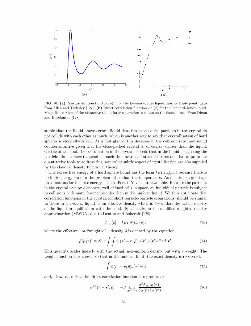
0.5 1 1.5 2 2.5 3 3.50

0.5

1

1.5

2

2.5

3

r/σ

g(r

)

(a) (b)

FIG. 10. (a) Pair-distribution function g(r) for the Lennard-Jones liquid near its triple point, data

from Allen and Tildesley [127]. (b) Direct correlation function c(2)(r) for the Lennard-Jones liquid.

Magnified version of the attractive tail at large separation is shown as the dashed line. From Dixon

and Hutchinson [128].

stable than the liquid above certain liquid densities because the particles in the crystal do

not collide with each other as much, which is another way to say that crystallisation of hard

spheres is sterically-driven. At a first glance, this decrease in the collision rate may sound

counter-intuitive given that the close-packed crystal is, of course, denser than the liquid.

On the other hand, the coordination in the crystal exceeds that in the liquid, suggesting the

particles do not have to spend as much time near each other. It turns out that appropriate

quantitative tools to address this, somewhat subtle aspect of crystallisation are also supplied

by the classical density functional theory.

The excess free energy of a hard sphere liquid has the form kBTfliq(ρliq) because there is

no finite energy scale in the problem other than the temperature. As mentioned, good ap-

proximations for this free energy, such as Percus-Yevick, are available. Because the particles

in the crystal occupy disparate, well defined cells in space, an individual particle is subject

to collisions with many fewer molecules than in the uniform liquid. We thus anticipate that

correlation functions in the crystal, for short particle-particle separations, should be similar

to those in a uniform liquid at an effective density which is lower that the actual density

of the liquid in equilibrium with the solid. Specifically, in the modified-weighted density

approximation (MWDA) due to Denton and Ashcroft [129]:

Fex [ρ] = kBTNfliq (ρ) , (73)

where the effective—or “weighted”—density ρ is defined by the equation:

ρ [ρ (r)] ≡ N−1

∫ ∫w (r′ − r; ρ) ρ (r) ρ (r′) d3rd3r′. (74)

This quantity scales linearly with the actual, non-uniform density but with a weight. The

weight function w is chosen so that in the uniform limit, the exact density is recovered:∫w(r′ − r; ρ)d3r′ = 1 (75)

and, likewise, so that the direct correlation function is reproduced:

c(2) (r − r′; ρ) = −β limρ(r)→ρ

δ2Fex [ρ (r)]

δρ (r) δρ (r′)(76)

34

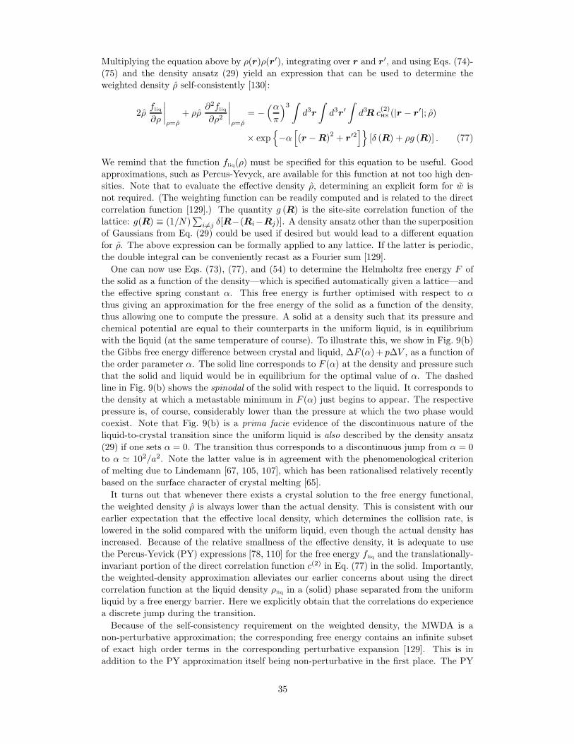
Multiplying the equation above by ρ(r)ρ(r′), integrating over r and r′, and using Eqs. (74)-

(75) and the density ansatz (29) yield an expression that can be used to determine the

weighted density ρ self-consistently [130]:

2ρfliq

∂ρ

∣∣∣∣ρ=ρ

+ ρρ∂2fliq

∂ρ2

∣∣∣∣ρ=ρ

= −(απ

)3 ∫d3r

∫d3r′

∫d3R c

(2)HS (|r − r′|; ρ)

× exp−α[(r −R)

2+ r′2

][δ (R) + ρg (R)] . (77)

We remind that the function fliq(ρ) must be specified for this equation to be useful. Good

approximations, such as Percus-Yevyck, are available for this function at not too high den-

sities. Note that to evaluate the effective density ρ, determining an explicit form for w is

not required. (The weighting function can be readily computed and is related to the direct

correlation function [129].) The quantity g (R) is the site-site correlation function of the

lattice: g(R) ≡ (1/N)∑

i6=j δ[R−(Ri−Rj)]. A density ansatz other than the superposition

of Gaussians from Eq. (29) could be used if desired but would lead to a different equation

for ρ. The above expression can be formally applied to any lattice. If the latter is periodic,

the double integral can be conveniently recast as a Fourier sum [129].

One can now use Eqs. (73), (77), and (54) to determine the Helmholtz free energy F of

the solid as a function of the density—which is specified automatically given a lattice—and

the effective spring constant α. This free energy is further optimised with respect to α

thus giving an approximation for the free energy of the solid as a function of the density,

thus allowing one to compute the pressure. A solid at a density such that its pressure and

chemical potential are equal to their counterparts in the uniform liquid, is in equilibrium

with the liquid (at the same temperature of course). To illustrate this, we show in Fig. 9(b)

the Gibbs free energy difference between crystal and liquid, ∆F (α) + p∆V , as a function of

the order parameter α. The solid line corresponds to F (α) at the density and pressure such

that the solid and liquid would be in equilibrium for the optimal value of α. The dashed

line in Fig. 9(b) shows the spinodal of the solid with respect to the liquid. It corresponds to

the density at which a metastable minimum in F (α) just begins to appear. The respective

pressure is, of course, considerably lower than the pressure at which the two phase would

coexist. Note that Fig. 9(b) is a prima facie evidence of the discontinuous nature of the

liquid-to-crystal transition since the uniform liquid is also described by the density ansatz

(29) if one sets α = 0. The transition thus corresponds to a discontinuous jump from α = 0

to α ≃ 102/a2. Note the latter value is in agreement with the phenomenological criterion

of melting due to Lindemann [67, 105, 107], which has been rationalised relatively recently

based on the surface character of crystal melting [65].

It turns out that whenever there exists a crystal solution to the free energy functional,

the weighted density ρ is always lower than the actual density. This is consistent with our

earlier expectation that the effective local density, which determines the collision rate, is

lowered in the solid compared with the uniform liquid, even though the actual density has

increased. Because of the relative smallness of the effective density, it is adequate to use

the Percus-Yevick (PY) expressions [78, 110] for the free energy fliq and the translationally-

invariant portion of the direct correlation function c(2) in Eq. (77) in the solid. Importantly,

the weighted-density approximation alleviates our earlier concerns about using the direct

correlation function at the liquid density ρliq in a (solid) phase separated from the uniform

liquid by a free energy barrier. Here we explicitly obtain that the correlations do experience

a discrete jump during the transition.

Because of the self-consistency requirement on the weighted density, the MWDA is a

non-perturbative approximation; the corresponding free energy contains an infinite subset

of exact high order terms in the corresponding perturbative expansion [129]. This is in

addition to the PY approximation itself being non-perturbative in the first place. The PY

35

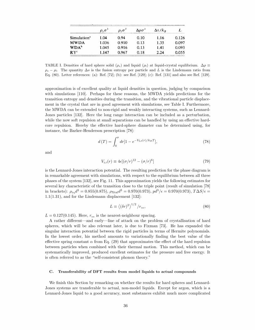
TABLE I. Densities of hard sphere solid (ρs) and liquid (ρl) at liquid-crystal equilibrium. ∆ρ ≡

ρs − ρl. The quantity ∆s is the fusion entropy per particle and L is the Lindemann ratio from

Eq. (80). Letter references: (a): Ref. [72]; (b): see Ref. [129]; (c): Ref. [131] and also see Ref. [129].

approximation is of excellent quality at liquid densities in question, judging by comparison

with simulations [110]. Perhaps for these reasons, the MWDA yields predictions for the

transition entropy and densities during the transition, and the vibrational particle displace-

ment in the crystal that are in good agreement with simulations, see Table I. Furthermore,

the MWDA can be extended to non-rigid and weakly interacting systems, such as Lennard-

Jones particles [132]. Here the long range interaction can be included as a perturbation,

while the now soft repulsion at small separations can be handled by using an effective hard-

core repulsion. Hereby the effective hard-sphere diameter can be determined using, for

instance, the Barker-Henderson prescription [78]:

d (T ) =

∫ σ

0

dr[1 − e−VLJ(r)/kBT ], (78)

and

VLJ(r) ≡ 4ǫ[(σ/r)12 − (σ/r)6] (79)

is the Lennard-Jones interaction potential. The resulting prediction for the phase diagram is

in remarkable agreement with simulations, with respect to the equilibrium between all three

phases of the system [132], see Fig. 11. This approximation yields the following estimates for

several key characteristic of the transition close to the triple point (result of simulation [78]

in brackets): ρliqd3 = 0.855(0.875), ρXtald

3 = 0.970(0.973), pd3/ǫ = 0.970(0.973), T∆S/ǫ =

1.1(1.31), and for the Lindemann displacement [132]:

L ≡⟨(δr)2

⟩1/2/rnn, (80)

L = 0.127(0.145). Here, rnn is the nearest-neighbour spacing.

A rather different—and early—line of attack on the problem of crystallisation of hard

spheres, which will be also relevant later, is due to Fixman [73]. He has expanded the

singular interaction potential between the rigid particles in terms of Hermite polynomials.

In the lowest order, his method amounts to variationally finding the best value of the

effective spring constant α from Eq. (29) that approximates the effect of the hard repulsion

between particles when combined with their thermal motion. This method, which can be

systematically improved, produced excellent estimates for the pressure and free energy. It

is often referred to as the “self-consistent phonon theory.”

C. Transferability of DFT results from model liquids to actual compounds

We finish this Section by remarking on whether the results for hard spheres and Lennard-

Jones systems are transferable to actual, non-model liquids. Except for argon, which is a

Lennard-Jones liquid to a good accuracy, most substances exhibit much more complicated

36

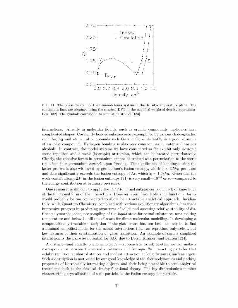
FIG. 11. The phase diagram of the Lennard-Jones system in the density-temperature plane. The

continuous lines are obtained using the classical DFT in the modified weighted density approxima-

tion [132]. The symbols correspond to simulation studies [133].

interactions. Already in molecular liquids, such as organic compounds, molecules have

complicated shapes. Covalently bonded substances are exemplified by various chalcogenides,

such As2Se3 and elemental compounds such Ge and Si, while ZnCl2 is a good example

of an ionic compound. Hydrogen bonding is also very common, as in water and various

alcohols. In contrast, the model systems we have considered so far exhibit only isotropic

steric repulsion and a weak (isotropic) attraction, which can be treated perturbatively.

Clearly, the cohesive forces in germanium cannot be treated as a perturbation to the steric

repulsion since germanium expands upon freezing. The significance of bonding during the

latter process is also witnessed by germanium’s fusion entropy, which is ∼ 3.5kB per atom

and thus significantly exceeds the fusion entropy of Ar, which is ∼ 1.68kB. Generally, the

work contribution p∆V in the fusion enthalpy (31) is very small—10−4 or so—compared to

the energy contribution at ordinary pressures.

One reason it is difficult to apply the DFT to actual substances is our lack of knowledge

of the functional form of the interactions. However, even if available, such functional forms

would probably be too complicated to allow for a tractable analytical approach. Inciden-

tally, while Quantum Chemistry, combined with various evolutionary algorithms, has made

impressive progress in predicting structures of solids and assessing relative stability of dis-

tinct polymorphs, adequate sampling of the liquid state for actual substances near melting

temperature and below is still out of reach for direct molecular modelling. In developing a

computationally-tractable description of the glass transition, our best bet may be to find

a minimal simplified model for the actual interactions that can reproduce only select, but

key features of their crystallisation or glass transition. An example of such a simplified

interaction is the pairwise potential for SiO2 due to Beest, Kramer, and Santen [134].

A distinct—and equally phenomenological—approach is to ask whether we can make a

correspondence between the actual substances and isotropically interacting particles that

exhibit repulsion at short distances and modest attraction at long distances, such as argon.

Such a description is motivated by our good knowledge of the thermodynamics and packing

properties of isotropically interacting objects, and their being amenable to semi-analytical

treatments such as the classical density functional theory. The key dimensionless number

characterising crystallisation of such particles is the fusion entropy per particle.

37

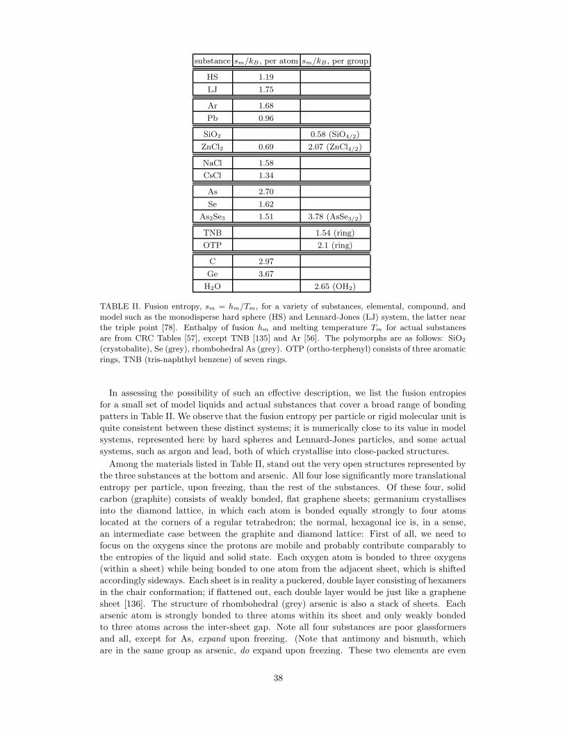
substance sm/kB , per atom sm/kB , per group

HS 1.19

LJ 1.75

Ar 1.68

Pb 0.96

SiO2 0.58 (SiO4/2)

ZnCl2 0.69 2.07 (ZnCl4/2)

NaCl 1.58

CsCl 1.34

As 2.70

Se 1.62

As2Se3 1.51 3.78 (AsSe3/2)

TNB 1.54 (ring)

OTP 2.1 (ring)

C 2.97

Ge 3.67

H2O 2.65 (OH2)

TABLE II. Fusion entropy, sm = hm/Tm, for a variety of substances, elemental, compound, and

model such as the monodisperse hard sphere (HS) and Lennard-Jones (LJ) system, the latter near

the triple point [78]. Enthalpy of fusion hm and melting temperature Tm for actual substances

are from CRC Tables [57], except TNB [135] and Ar [56]. The polymorphs are as follows: SiO2

(crystobalite), Se (grey), rhombohedral As (grey). OTP (ortho-terphenyl) consists of three aromatic

rings, TNB (tris-naphthyl benzene) of seven rings.

In assessing the possibility of such an effective description, we list the fusion entropies

for a small set of model liquids and actual substances that cover a broad range of bonding

patters in Table II. We observe that the fusion entropy per particle or rigid molecular unit is

quite consistent between these distinct systems; it is numerically close to its value in model

systems, represented here by hard spheres and Lennard-Jones particles, and some actual

systems, such as argon and lead, both of which crystallise into close-packed structures.

Among the materials listed in Table II, stand out the very open structures represented by

the three substances at the bottom and arsenic. All four lose significantly more translational

entropy per particle, upon freezing, than the rest of the substances. Of these four, solid

carbon (graphite) consists of weakly bonded, flat graphene sheets; germanium crystallises

into the diamond lattice, in which each atom is bonded equally strongly to four atoms

located at the corners of a regular tetrahedron; the normal, hexagonal ice is, in a sense,

an intermediate case between the graphite and diamond lattice: First of all, we need to

focus on the oxygens since the protons are mobile and probably contribute comparably to

the entropies of the liquid and solid state. Each oxygen atom is bonded to three oxygens

(within a sheet) while being bonded to one atom from the adjacent sheet, which is shifted

accordingly sideways. Each sheet is in reality a puckered, double layer consisting of hexamers

in the chair conformation; if flattened out, each double layer would be just like a graphene

sheet [136]. The structure of rhombohedral (grey) arsenic is also a stack of sheets. Each

arsenic atom is strongly bonded to three atoms within its sheet and only weakly bonded

to three atoms across the inter-sheet gap. Note all four substances are poor glassformers

and all, except for As, expand upon freezing. (Note that antimony and bismuth, which

are in the same group as arsenic, do expand upon freezing. These two elements are even

38

worse glassformers and better electric conductors than As.) To avoid confusion we note that

having relatively little entropy per atom does not guarantee being a good glass-former, as

can be seen by comparing NaCl and CsCl (poor glass-formers forming a simple-cubic-like

and BCC-like structures respectively) and ZnCl2 and As2Se3, the latter two being good

glass-formers. Zinc chloride consists of relatively rigid, corner-sharing ZnCl4/2 tetrahedra

(but apparently not as rigid as in SiO4/2) while As2Se3 consists of relatively rigid AsSe3/2pyramids co-joined through the Se corners and forming puckered sheets like those of black

phosphorus but with vacancies [29].

To appreciate just how open the diamond structure is, and to rationalise its high fusion

entropy, we first consider the FCC lattice, which is a close-packed structure. The FCC

structure has two types of cavities: two octahedral (cornered by the six face-centred vertices)

per three tetrahedral. The diamond lattice can be produced from the FCC lattice by placing

a particle in every other tetrahedral cavity in a (3D) checker pattern. Alternatively, to

generate the diamond lattice, one can superimpose two identical FCC lattices, with lattice

constant 1, which are shifted by√3/4 along the main diagonal. On the other hand, the

simple-cubic lattice can be obtained by superimposing two identical FCC lattices, with

lattice constant 1, but which are shifted by√3/2 along the main diagonal. Consequently,

two diamond lattices complement each other to form a BCC lattice. Thus roughly, the

entropy of freezing of the diamond lattice is the total entropy due to the ordering of an

equal measure of particles and vacancies into a BCC lattice. Per particle, we get about

twice as much fusion entropy as for a BCC lattice made of two distinct particles. (We

should be mindful of the mixing entropy, too.) Indeed, the fusion entropy of CsCl per atom

is at least twice less than that of germanium or water. The high fusion entropy of open

structures is in full harmony with our earlier analysis of the discontinuous nature of the

liquid-to-crystal transition. Per that discussion, materials with open structures freeze well

before the steric effects—which are signalled by relatively low values of the fusion entropy—

become important. It is instructive to note that the filling fraction in the diamond lattice

made of touching, identical spheres is only π√3/16 ≈ 0.34, to be compared with the filling

fraction of the FCC lattice, π/3√2 ≈ 0.74, or the random close-packed structure, viz.,

≈ 0.64 [137]. Conversely, many example of pressure-induced amorphisation of relatively

open structures are known [138–141].

We thus tentatively conclude that with the exception of these very open structures, steric

interactions contribute significantly to the thermodynamics of freezing. The degree of “open-

ness” is positively correlated—but not without exception—with the sign of the volume

change during freezing and the value of the fusion entropy; it is negatively correlated with

the glass-forming ability. We will be able to rationalise this negative correlation in the fol-

lowing Section, where we show that equilibrium aperiodic structures are stabilised by steric

effects. Now, the glass forming ability is also decreased when a relatively well-packed struc-

ture is agreeable with the stoichiometry, even if the fusion entropy is not too high. (The

rock salt structure is, in fact, rather well-packed for NaCl, because of the disparity in the

ion sizes and despite the relatively low coordination number of six.) Thus it appears that

at least for structures that are not too open, an effective description in terms isotropically

interacting particles is possible. Certain layered compounds, such as As2Se3, are good glass-

formers despite having a relatively large entropy of fusion. We shall see that determining

the effective particle size for such compounds is difficult, in contrast with compounds that

exhibit less propensity for local ordering.

To avoid confusion, we note that substances with very isotropic bonding, such as monodis-

perse hard-spheres or Lennard-Jones particles, are also poor glassformers. These fail to

vitrify readily despite the prominence of steric effects because monodisperse spheres easily

find close-packed arrangements. We will return to this topic at the end of the article.

39

IV. EMERGENCE OF APERIODIC CRYSTAL AND ACTIVATED TRANSPORT,

AS A BREAKING OF TRANSLATIONAL SYMMETRY

The density functional theory (DFT) provides us with reliable tools to determine the free

energy of the uniform liquid and, at the same time, the free energy of specific crystalline

arrangements. As such, the DFT enables us to assess the stability of distinct crystalline

polymorphs relative to each other and to the uniform liquid state in the first place. Likewise,

it will enable us to assess the stability of aperiodic structures. Until further notice, we will

focus on rigid systems exemplified by hard spheres and also with added weak attraction

as in Lennard-Jones liquids. These results will be generalised for actual substances in due

time.

A. The Random First Order Transition (RFOT)

Let us now consider a supercooled liquid just above its glass transition, so that its struc-

ture relaxes on a timescale comparable to one hour. The latter time scale is 16 orders of

magnitude longer than the vibrational relaxation time, which is numerically a picosecond

or so. In other words, the supercooled liquid, despite being able to flow on very long times,

is a solid on mesoscopic length scales and below. Frozen glasses, if quenched considerably

below the glass transition, not only fail to flow but are often even more rigid than the

corresponding crystal. Given their remarkable mechanical stability, it is natural to enquire

whether aperiodic structures such as those pertaining to supercooled liquids or glasses are

free energy minima.

This question was answered affirmatively by Stoessel and Wolynes in 1984 [142], who

used the self-consistent phonon theory and assumed an aperiodic structure characterised by

the pair-correlation function g(r) of a uniform liquid. These authors have determined self-

consistently the force constant α from the Gaussian density profile (29), where the lattice

is now aperiodic. The self-consistent phonon theory also predicts the liquid density above

which the aperiodic free energy minima begin to exist.

Soon afterwards, Singh, Stoessel, Wolynes [143] (SSW) reported their stability analysis of

aperiodic structures using the Ramakrishnan-Yussouff density functional (52), in which the

free energy was determined explicitly as a function of α, analogously to the periodic-crystal

calculation in Fig. 9(b). There are notable differences between how the calculations are set

up in the periodic and aperiodic case, in addition to the use of an aperiodic lattice. (SSW

employed a lattice generated using the Bennett algorithm [144].) In the regular liquid-

to-crystal transition, the two phases occupy distinct parts of the space. The two phases

can coexist for an indefinite time, if the temperature, pressure, and chemical potential

are uniform throughout the whole system. The appropriate free energy for analysing the

relative stability of the two phases is thus the Gibbs free energy. One may still consider a

transient coexistence between the two phases when one of them is metastable, and so only

temperatures and pressures are equal between the two phases, while the metastable free

energy is now in excess of the Gibbs free energy. (The metastable phase will eventually

convert into the stable phase, subject to pertinent kinetics.) In contrast, there is no phase

separation in the aperiodic case. The aperiodic minimum at finite α is built with the very

same particles comprising the liquid and thus replaces the uniform liquid, it does not coexist

with the uniform liquid; there is no spatial interface involved. Nor is there volume change

and so the appropriate free energy is the Helmholtz free energy from Eq. (14).

The result of the SSW calculation of the free energy F (α) for an aperiodic lattice, relative

to the uniform liquid is shown in Fig. 12(a). Here we observe that in complete analogy with

the regular liquid-to-crystal transition, a metastable minimum develops at a finite value of

40

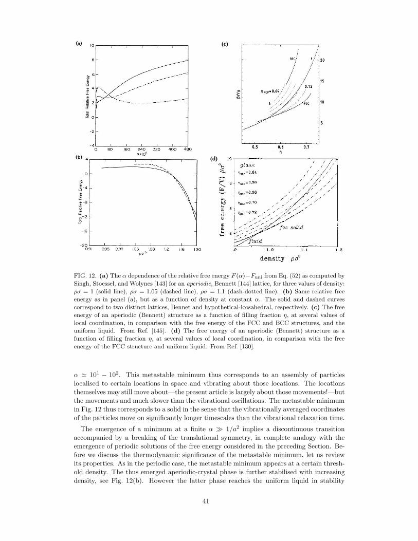
(d)

(c)

FIG. 12. (a) The α dependence of the relative free energy F (α)−Funi from Eq. (52) as computed by

Singh, Stoessel, and Wolynes [143] for an aperiodic, Bennett [144] lattice, for three values of density:

ρσ = 1 (solid line), ρσ = 1.05 (dashed line), ρσ = 1.1 (dash-dotted line). (b) Same relative free

energy as in panel (a), but as a function of density at constant α. The solid and dashed curves

correspond to two distinct lattices, Bennet and hypothetical-icosahedral, respectively. (c) The free

energy of an aperiodic (Bennett) structure as a function of filling fraction η, at several values of

local coordination, in comparison with the free energy of the FCC and BCC structures, and the

uniform liquid. From Ref. [145]. (d) The free energy of an aperiodic (Bennett) structure as a

function of filling fraction η, at several values of local coordination, in comparison with the free

energy of the FCC structure and uniform liquid. From Ref. [130].

α ≃ 101 − 102. This metastable minimum thus corresponds to an assembly of particles

localised to certain locations in space and vibrating about those locations. The locations

themselves may still move about—the present article is largely about those movements!—but

the movements and much slower than the vibrational oscillations. The metastable minimum

in Fig. 12 thus corresponds to a solid in the sense that the vibrationally averaged coordinates

of the particles move on significantly longer timescales than the vibrational relaxation time.

The emergence of a minimum at a finite α ≫ 1/a2 implies a discontinuous transition

accompanied by a breaking of the translational symmetry, in complete analogy with the

emergence of periodic solutions of the free energy considered in the preceding Section. Be-

fore we discuss the thermodynamic significance of the metastable minimum, let us review

its properties. As in the periodic case, the metastable minimum appears at a certain thresh-

old density. The thus emerged aperiodic-crystal phase is further stabilised with increasing

density, see Fig. 12(b). However the latter phase reaches the uniform liquid in stability

41

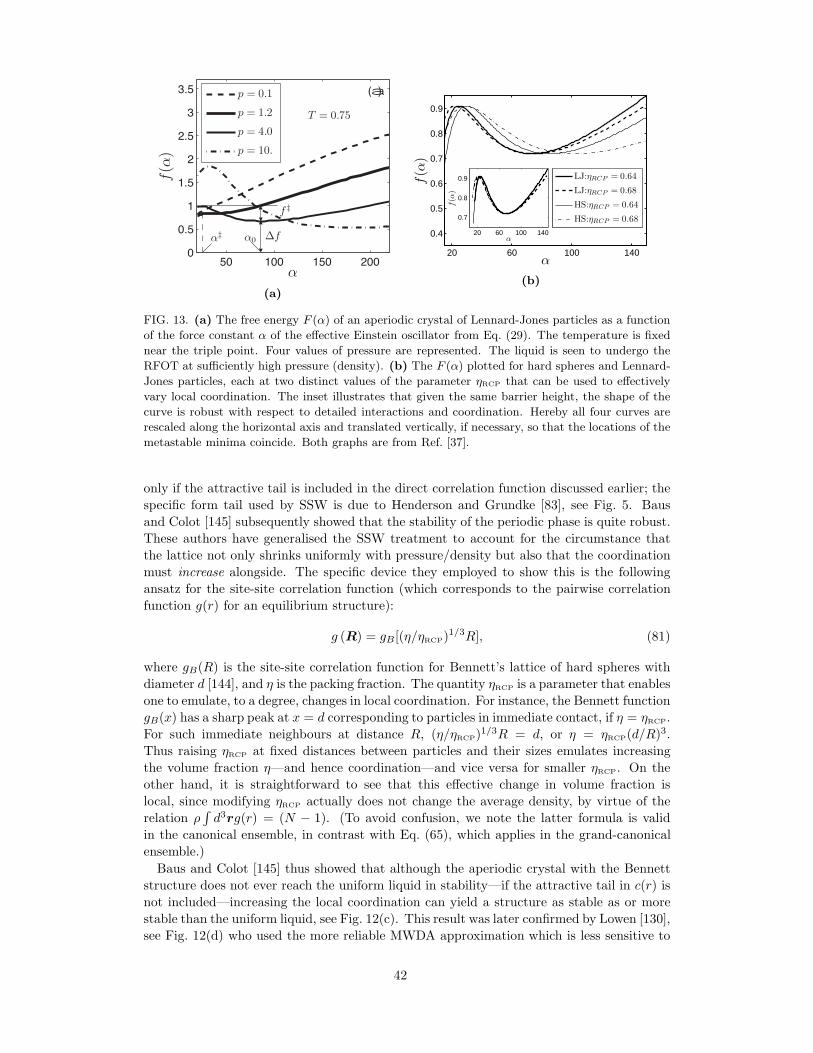
50 100 150 2000

0.5

1

1.5

2

2.5

3

3.5

α

f(α

)

0

0.5

1

1.5

2

2.5

3

3.5p = 0.1

p = 1.2

p = 4.0

p = 10.

(a)

f ‡

∆fα0α‡

T = 0.75

(a)

20 60 100 140

0.4

0.5

0.6

0.7

0.8

0.9

α

f(α

)

20 60 100 140

0.7

0.8

0.9

α

f(α

)

LJ:ηRCP = 0.64

LJ:ηRCP = 0.68

HS:ηRCP = 0.64

HS:ηRCP = 0.68

(b)

FIG. 13. (a) The free energy F (α) of an aperiodic crystal of Lennard-Jones particles as a function

of the force constant α of the effective Einstein oscillator from Eq. (29). The temperature is fixed

near the triple point. Four values of pressure are represented. The liquid is seen to undergo the

RFOT at sufficiently high pressure (density). (b) The F (α) plotted for hard spheres and Lennard-

Jones particles, each at two distinct values of the parameter ηRCP that can be used to effectively

vary local coordination. The inset illustrates that given the same barrier height, the shape of the

curve is robust with respect to detailed interactions and coordination. Hereby all four curves are

rescaled along the horizontal axis and translated vertically, if necessary, so that the locations of the

metastable minima coincide. Both graphs are from Ref. [37].

only if the attractive tail is included in the direct correlation function discussed earlier; the

specific form tail used by SSW is due to Henderson and Grundke [83], see Fig. 5. Baus

and Colot [145] subsequently showed that the stability of the periodic phase is quite robust.

These authors have generalised the SSW treatment to account for the circumstance that

the lattice not only shrinks uniformly with pressure/density but also that the coordination

must increase alongside. The specific device they employed to show this is the following

ansatz for the site-site correlation function (which corresponds to the pairwise correlation

function g(r) for an equilibrium structure):

g (R) = gB[(η/ηRCP)1/3R], (81)

where gB(R) is the site-site correlation function for Bennett’s lattice of hard spheres with

diameter d [144], and η is the packing fraction. The quantity ηRCP is a parameter that enables

one to emulate, to a degree, changes in local coordination. For instance, the Bennett function

gB(x) has a sharp peak at x = d corresponding to particles in immediate contact, if η = ηRCP.

For such immediate neighbours at distance R, (η/ηRCP)1/3R = d, or η = ηRCP(d/R)

3.

Thus raising ηRCP at fixed distances between particles and their sizes emulates increasing

the volume fraction η—and hence coordination—and vice versa for smaller ηRCP. On the

other hand, it is straightforward to see that this effective change in volume fraction is

local, since modifying ηRCP actually does not change the average density, by virtue of the

relation ρ∫d3rg(r) = (N − 1). (To avoid confusion, we note the latter formula is valid

in the canonical ensemble, in contrast with Eq. (65), which applies in the grand-canonical

ensemble.)

Baus and Colot [145] thus showed that although the aperiodic crystal with the Bennett

structure does not ever reach the uniform liquid in stability—if the attractive tail in c(r) is

not included—increasing the local coordination can yield a structure as stable as or more

stable than the uniform liquid, see Fig. 12(c). This result was later confirmed by Lowen [130],

see Fig. 12(d) who used the more reliable MWDA approximation which is less sensitive to

42

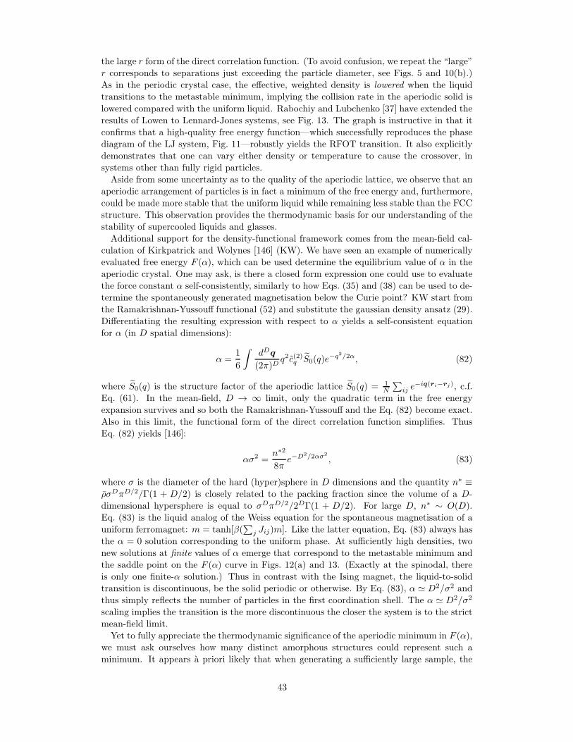
the large r form of the direct correlation function. (To avoid confusion, we repeat the “large”

r corresponds to separations just exceeding the particle diameter, see Figs. 5 and 10(b).)

As in the periodic crystal case, the effective, weighted density is lowered when the liquid

transitions to the metastable minimum, implying the collision rate in the aperiodic solid is

lowered compared with the uniform liquid. Rabochiy and Lubchenko [37] have extended the

results of Lowen to Lennard-Jones systems, see Fig. 13. The graph is instructive in that it

confirms that a high-quality free energy function—which successfully reproduces the phase

diagram of the LJ system, Fig. 11—robustly yields the RFOT transition. It also explicitly

demonstrates that one can vary either density or temperature to cause the crossover, in

systems other than fully rigid particles.

Aside from some uncertainty as to the quality of the aperiodic lattice, we observe that an

aperiodic arrangement of particles is in fact a minimum of the free energy and, furthermore,

could be made more stable that the uniform liquid while remaining less stable than the FCC

structure. This observation provides the thermodynamic basis for our understanding of the

stability of supercooled liquids and glasses.

Additional support for the density-functional framework comes from the mean-field cal-

culation of Kirkpatrick and Wolynes [146] (KW). We have seen an example of numerically

evaluated free energy F (α), which can be used determine the equilibrium value of α in the

aperiodic crystal. One may ask, is there a closed form expression one could use to evaluate

the force constant α self-consistently, similarly to how Eqs. (35) and (38) can be used to de-

termine the spontaneously generated magnetisation below the Curie point? KW start from

the Ramakrishnan-Yussouff functional (52) and substitute the gaussian density ansatz (29).

Differentiating the resulting expression with respect to α yields a self-consistent equation

for α (in D spatial dimensions):

α =1

6

∫dDq

(2π)Dq2c(2)q S0(q)e

−q2/2α, (82)

where S0(q) is the structure factor of the aperiodic lattice S0(q) = 1N

∑ij e

−iq(ri−rj), c.f.

Eq. (61). In the mean-field, D → ∞ limit, only the quadratic term in the free energy

expansion survives and so both the Ramakrishnan-Yussouff and the Eq. (82) become exact.

Also in this limit, the functional form of the direct correlation function simplifies. Thus

Eq. (82) yields [146]:

ασ2 =n∗2

8πe−D2/2ασ2

, (83)

where σ is the diameter of the hard (hyper)sphere in D dimensions and the quantity n∗ ≡ρσDπD/2/Γ(1 + D/2) is closely related to the packing fraction since the volume of a D-

dimensional hypersphere is equal to σDπD/2/2DΓ(1 + D/2). For large D, n∗ ∼ O(D).

Eq. (83) is the liquid analog of the Weiss equation for the spontaneous magnetisation of a

uniform ferromagnet: m = tanh[β(∑

j Jij)m]. Like the latter equation, Eq. (83) always has

the α = 0 solution corresponding to the uniform phase. At sufficiently high densities, two

new solutions at finite values of α emerge that correspond to the metastable minimum and

the saddle point on the F (α) curve in Figs. 12(a) and 13. (Exactly at the spinodal, there

is only one finite-α solution.) Thus in contrast with the Ising magnet, the liquid-to-solid

transition is discontinuous, be the solid periodic or otherwise. By Eq. (83), α ≃ D2/σ2 and

thus simply reflects the number of particles in the first coordination shell. The α ≃ D2/σ2

scaling implies the transition is the more discontinuous the closer the system is to the strict

mean-field limit.

Yet to fully appreciate the thermodynamic significance of the aperiodic minimum in F (α),

we must ask ourselves how many distinct amorphous structures could represent such a

minimum. It appears a priori likely that when generating a sufficiently large sample, the

43

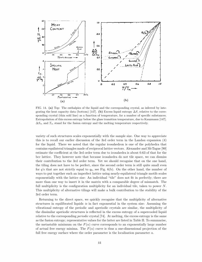
(a) (b)

FIG. 14. (a) Top: The enthalpies of the liquid and the corresponding crystal, as inferred by inte-

grating the heat capacity data (bottom) [147]. (b) Excess liquid entropy ∆S, relative to the corre-

sponding crystal (thin sold line) as a function of temperature, for a number of specific substances.

Extrapolation of this excess entropy below the glass transition temperature, due to Kauzmann [147].

∆Sm and Tm stand for the fusion entropy and the melting temperature respectively.

variety of such structures scales exponentially with the sample size. One way to appreciate

this is to recall our earlier discussion of the 3rd order term in the Landau expansion (4)

for the liquid. There we noted that the regular icosahedron is one of the polyhedra that

contains equilateral triangles made of reciprocal lattice vectors. Alexander and McTague [90]

estimate the coefficient at the 3rd order term due to icosahedra is about 0.63 of that for the

bcc lattice. They however note that because icosahedra do not tile space, we can dismiss

their contribution to the 3rd order term. Yet we should recognise that on the one hand,

the tiling does not have to be perfect, since the second order term is still quite small even

for q’s that are not strictly equal to q0, see Fig. 6(b). On the other hand, the number of

ways to put together such an imperfect lattice using nearly-equilateral triangle motifs scales

exponentially with the lattice size: An individual “tile” does not fit in perfectly; there are

more than one way to insert it in the matrix with a comparable degree of mismatch. The

full multiplicity is the configuration multiplicity for an individual tile, taken to power N .

This multiplicity of alternative tilings will make a bulk contribution to the stability of the

3rd order term.

Returning to the direct space, we quickly recognise that the multiplicity of alternative

structures in equilibrated liquids is in fact exponential in the system size: Assuming the

vibrational entropy of the periodic and aperiodic crystals are similar, the multiplicity of

the dissimilar aperiodic structures is reflected in the excess entropy of a supercooled liquid

relative to the corresponding periodic crystal [74]. At melting, the excess entropy is the same

as the fusion entropy; representative values for the latter are listed in Table II. To summarise,

the metastable minimum on the F (α) curve corresponds to an exponentially large number

of actual free energy minima. The F (α) curve is thus a one-dimensional projection of the

full free energy surface where the order parameter is the localisation parameter α.

44

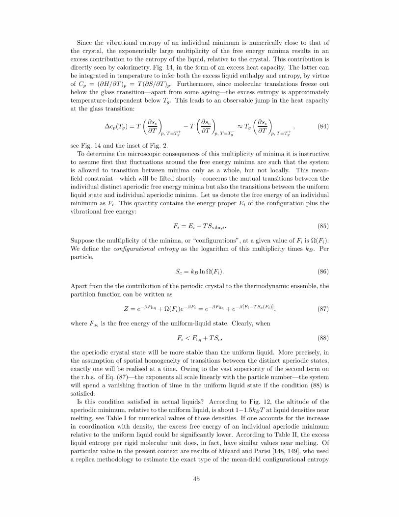
Since the vibrational entropy of an individual minimum is numerically close to that of

the crystal, the exponentially large multiplicity of the free energy minima results in an

excess contribution to the entropy of the liquid, relative to the crystal. This contribution is

directly seen by calorimetry, Fig. 14, in the form of an excess heat capacity. The latter can

be integrated in temperature to infer both the excess liquid enthalpy and entropy, by virtue

of Cp = (∂H/∂T )p = T (∂S/∂T )p. Furthermore, since molecular translations freeze out

below the glass transition—apart from some ageing—the excess entropy is approximately

temperature-independent below Tg. This leads to an observable jump in the heat capacity

at the glass transition:

∆cp(Tg) = T

(∂sc∂T

)

p, T=T+g

− T

(∂sc∂T

)

p, T=T−g

≈ Tg

(∂sc∂T

)

p, T=T+g

, (84)

see Fig. 14 and the inset of Fig. 2.

To determine the microscopic consequences of this multiplicity of minima it is instructive

to assume first that fluctuations around the free energy minima are such that the system

is allowed to transition between minima only as a whole, but not locally. This mean-

field constraint—which will be lifted shortly—concerns the mutual transitions between the

individual distinct aperiodic free energy minima but also the transitions between the uniform

liquid state and individual aperiodic minima. Let us denote the free energy of an individual

minimum as Fi. This quantity contains the energy proper Ei of the configuration plus the

vibrational free energy:

Fi = Ei − TSvibr,i. (85)

Suppose the multiplicity of the minima, or “configurations”, at a given value of Fi is Ω(Fi).

We define the configurational entropy as the logarithm of this multiplicity times kB. Per

particle,

Sc = kB lnΩ(Fi). (86)

Apart from the the contribution of the periodic crystal to the thermodynamic ensemble, the

partition function can be written as

Z = e−βFliq +Ω(Fi)e−βFi = e−βFliq + e−β[Fi−TSc(Fi)], (87)

where Fliq is the free energy of the uniform-liquid state. Clearly, when

Fi < Fliq + TSc, (88)

the aperiodic crystal state will be more stable than the uniform liquid. More precisely, in

the assumption of spatial homogeneity of transitions between the distinct aperiodic states,

exactly one will be realised at a time. Owing to the vast superiority of the second term on

the r.h.s. of Eq. (87)—the exponents all scale linearly with the particle number—the system

will spend a vanishing fraction of time in the uniform liquid state if the condition (88) is

satisfied.

Is this condition satisfied in actual liquids? According to Fig. 12, the altitude of the

aperiodic minimum, relative to the uniform liquid, is about 1−1.5kBT at liquid densities near

melting, see Table I for numerical values of those densities. If one accounts for the increase

in coordination with density, the excess free energy of an individual aperiodic minimum

relative to the uniform liquid could be significantly lower. According to Table II, the excess

liquid entropy per rigid molecular unit does, in fact, have similar values near melting. Of

particular value in the present context are results of Mezard and Parisi [148, 149], who used

a replica methodology to estimate the exact type of the mean-field configurational entropy

45

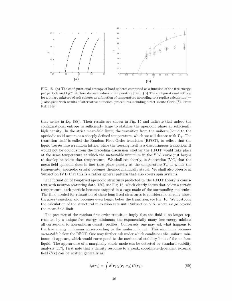
1.5 2.0 2.5 3.0 3.5f

0.0

0.5

1.0

1.5

Sc

(a)

0

0.2

0.4

0.6

0.8

1

1.2

1.4

1.6

1.8

0 0.05 0.1 0.15 0.2 0.25 0.3 0.35 0.4 0.45 0.5

Σ

T

(b)

FIG. 15. (a) The configurational entropy of hard spheres computed as a function of the free energy,

per particle and kBT , at three distinct values of temperature [148]. (b) The configurational entropy

for a binary mixture of soft spheres as a function of temperature according to a replica calculation(—

), alongside with results of alternative numerical procedures including direct Monte-Carlo (*). From

Ref. [149].

that enters in Eq. (88). Their results are shown in Fig. 15 and indicate that indeed the

configurational entropy is sufficiently large to stabilise the aperiodic phase at sufficiently

high density. In the strict mean-field limit, the transition from the uniform liquid to the

aperiodic solid occurs at a sharply defined temperature, which we will denote with TA. The

transition itself is called the Random First Order transition (RFOT), to reflect that the

liquid freezes into a random lattice, while the freezing itself is a discontinuous transition. It

would not be obvious from the preceding discussion whether the RFOT would take place

at the same temperature at which the metastable minimum in the F (α) curve just begins

to develop or below that temperature. We shall see shortly, in Subsection IVC, that the

mean-field spinodal does in fact take place exactly at the temperature TA at which the

(degenerate) aperiodic crystal becomes thermodynamically stable. We shall also observe in

Subsection IVD that this is a rather general pattern that also covers spin systems.

The formation of long-lived aperiodic structures predicted by the RFOT theory is consis-

tent with neutron scattering data [150], see Fig. 16, which clearly shows that below a certain

temperature, each particle becomes trapped in a cage made of the surrounding molecules.

The time needed for relaxation of these long-lived structures is considerable already above

the glass transition and becomes even longer below the transition, see Fig. 16. We postpone

the calculation of the structural relaxation rate until Subsection VA, where we go beyond

the mean-field limit.

The presence of the random first order transition imply that the fluid is no longer rep-

resented by a unique free energy minimum; the exponentially many free energy minima

all correspond to non-uniform density profiles. Conversely, one may ask what happens to

the free energy minimum corresponding to the uniform liquid. This minimum becomes

metastable below the RFOT. One may further ask under which conditions the uniform min-

imum disappears, which would correspond to the mechanical stability limit of the uniform

liquid. The appearance of a marginally stable mode can be detected by standard stability

analysis [117]. First note that a density response to a weak, coordinate-dependent external

field U(r) can be written generally as:

δρ(r1) =

∫d3r2 χ(r1, r2)U(r2). (89)

46

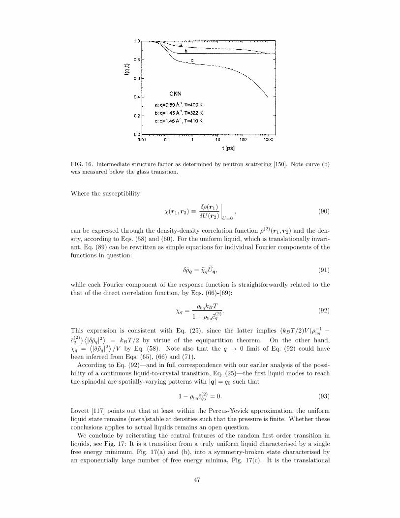
FIG. 16. Intermediate structure factor as determined by neutron scattering [150]. Note curve (b)

was measured below the glass transition.

Where the susceptibility:

χ(r1, r2) ≡δρ(r1)

δU(r2)

∣∣∣∣U=0

, (90)

can be expressed through the density-density correlation function ρ(2)(r1, r2) and the den-

sity, according to Eqs. (58) and (60). For the uniform liquid, which is translationally invari-

ant, Eq. (89) can be rewritten as simple equations for individual Fourier components of the

functions in question:

δρq = χqUq, (91)

while each Fourier component of the response function is straightforwardly related to the

that of the direct correlation function, by Eqs. (66)-(69):

χq =ρliqkBT

1− ρliqc(2)q

. (92)

This expression is consistent with Eq. (25), since the latter implies (kBT/2)V (ρ−1liq

−c(2)q )

⟨|δρq|2

⟩= kBT/2 by virtue of the equipartition theorem. On the other hand,

χq =⟨|δρq|2

⟩/V by Eq. (58). Note also that the q → 0 limit of Eq. (92) could have

been inferred from Eqs. (65), (66) and (71).

According to Eq. (92)—and in full correspondence with our earlier analysis of the possi-

bility of a continuous liquid-to-crystal transition, Eq. (25)—the first liquid modes to reach

the spinodal are spatially-varying patterns with |q| = q0 such that

1− ρliqc(2)q0 = 0. (93)

Lovett [117] points out that at least within the Percus-Yevick approximation, the uniform

liquid state remains (meta)stable at densities such that the pressure is finite. Whether these

conclusions applies to actual liquids remains an open question.

We conclude by reiterating the central features of the random first order transition in

liquids, see Fig. 17: It is a transition from a truly uniform liquid characterised by a single

free energy minimum, Fig. 17(a) and (b), into a symmetry-broken state characterised by

an exponentially large number of free energy minima, Fig. 17(c). It is the translational

47

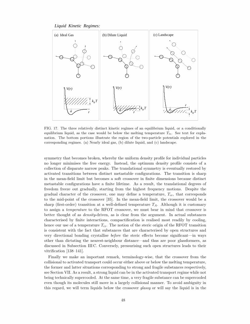
k TB

a

V(r)

rk TB

k TB

(c) Landscape(b) Dilute Liquid(a) Ideal Gas

Liquid Kinetic Regimes:

a

V(r)

a

V(r)

r

r

FIG. 17. The three relatively distinct kinetic regimes of an equilibrium liquid, or a conditionally

equilibrium liquid, as the case would be below the melting temperature Tm. See text for expla-

nation. The bottom portions illustrate the region of the two-particle potentials explored in the

corresponding regimes. (a) Nearly ideal gas, (b) dilute liquid, and (c) landscape.

symmetry that becomes broken, whereby the uniform density profile for individual particles

no longer minimises the free energy. Instead, the optimum density profile consists of a

collection of disparate narrow peaks. The translational symmetry is eventually restored by

activated transitions between distinct metastable configurations. The transition is sharp

in the mean-field limit but becomes a soft crossover in finite dimensions because distinct

metastable configurations have a finite lifetime. As a result, the translational degrees of

freedom freeze out gradually, starting from the highest frequency motions. Despite the

gradual character of the crossover, one may define a temperature, Tcr, that corresponds

to the mid-point of the crossover [35]. In the mean-field limit, the crossover would be a

sharp (first-order) transition at a well-defined temperature TA. Although it is customary

to assign a temperature to the RFOT crossover, we must bear in mind that crossover is

better thought of as density-driven, as is clear from the argument. In actual substances

characterised by finite interactions, compactification is realised most readily by cooling,

hence our use of a temperature Tcr. The notion of the steric origin of the RFOT transition

is consistent with the fact that substances that are characterised by open structures and

very directional bonding crystallise before the steric effects become significant—in ways

other than dictating the nearest-neighbour distance—and thus are poor glassformers, as

discussed in Subsection III C. Conversely, pressurising such open structures leads to their

vitrification [138–141].

Finally we make an important remark, terminology-wise, that the crossover from the

collisional to activated transport could occur either above or below the melting temperature,

the former and latter situations corresponding to strong and fragile substances respectively,

see Section VII. As a result, a strong liquid can be in the activated transport regime while not

being technically supercooled. At the same time, a very fragile substance can be supercooled

even though its molecules still move in a largely collisional manner. To avoid ambiguity in

this regard, we will term liquids below the crossover glassy or will say the liquid is in the

48

landscape regime.

B. Configurational Entropy

We just saw that the magnitude of the configurational entropy is key to whether the

emerging aperiodic structures can compete, free-energy wise, with the uniform liquid state.

We shall also see shortly that knowing the configurational entropy is central to computing

the activation barrier for liquid relaxations below the crossover. The configurational entropy

has been evaluated from first principles only for the simplest systems, even if approximately,

see Fig. 15. Such calculations for actual substances are very difficult, especially given that

the explicit form of the actual quantum-chemical interactions is complicated and not known

in closed form. On the other hand, the classical DFT calculations for aperiodic lattices,

from Subsection IVA, strictly apply only to isotropically interacting particles that repel at

short distances and attract modestly at large distances. It is thus imperative to be able

to take advantage of the measured excess liquid entropy of actual liquids, which, however,

must be calibrated in terms the entropy content of such a model liquid that is amenable to

the DFT analysis.

Before we discuss the calibration, we provide in Fig. 14(b) a graph of the excess liquid

entropy, as a function of temperature, from the seminal paper of Kauzmann [147]. Kauz-

mann emphasised, following Simon [151], that the excess entropy would vanish at a finite

temperature, TK > 0, if extrapolated beyond the glass transition. Approximately, one may

write:

sc ≈ ∆cp(TK)(T − TK)/TK . (94)

In practice, one often uses the following functional form for the temperature dependence of

the configurational entropy [152, 153]:

sc ≃ ∆cp(Tg)Tg(1/TK − 1/T ), (95)

c.f. Eq. (84), which works very well for many substances.

To calibrate the excess liquid entropy of an actual substance we first consider a useful,

extreme limit of the hard sphere: The entropy of monodisperse spheres depends only on the

density. Likewise, the fusion entropy is also temperature independent and is about 1.19kBper particle (Table I). Furthermore, we also understand fairly well how hard spheres pack:

For instance, the highest filling fraction for monodisperse spheres is π/3√2 ≈ 0.74. We

know accurately the density of the liquid and crystal in equilibrium (Table I), and have

a good idea as to the filling fraction of the random close-packed structure, 0.64 or so. A

somewhat better reference system can be obtained by starting with hard spheres and then

including a weakly attractive tail to the particle-particle interaction. The next step is to

find a naturally occurring system that shows strong—but not infinitely strong—repulsion at

short distances and weak attraction otherwise. The finiteness of the energy scale associated

with both the repulsive and attractive portion of the interaction affords one more flexibility

in calibrating actual interactions. (We have already seen an example of this in Section III,

see Fig. 11.) Argon is a good choice: On the one hand, Ar is a closed-shell atom and so

two argon atoms repel at short distances owing to the Pauli exclusion principle while being

attracted through weak, dispersive forces at larger separations. On the other hand, Ar is

not too light so quantum effects are not large, and it is not too heavy, so that polarizability

is not too high.

In all known glassformers—in contrast with argon—the interactions are directional, to

a lesser or greater degree. For instance, suppose the magnitude of the fusion entropy per

atom in an actual glass-former is smaller than in argon, see Table II. This means that fewer

49

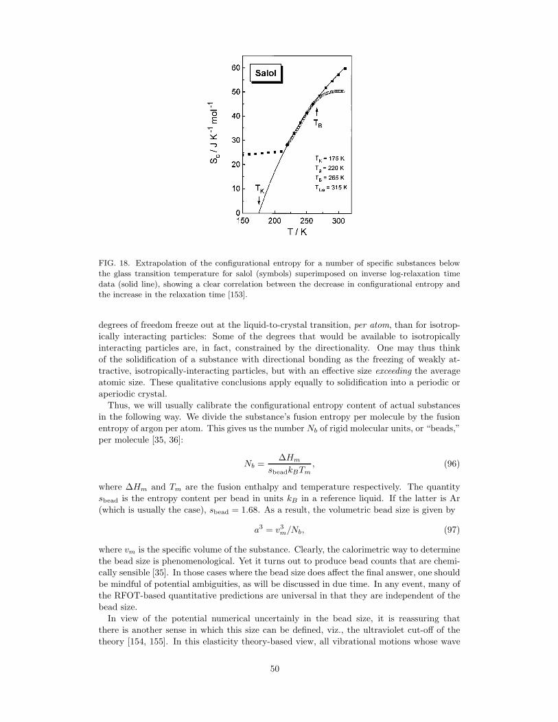
FIG. 18. Extrapolation of the configurational entropy for a number of specific substances below

the glass transition temperature for salol (symbols) superimposed on inverse log-relaxation time

data (solid line), showing a clear correlation between the decrease in configurational entropy and

the increase in the relaxation time [153].

degrees of freedom freeze out at the liquid-to-crystal transition, per atom, than for isotrop-

ically interacting particles: Some of the degrees that would be available to isotropically

interacting particles are, in fact, constrained by the directionality. One may thus think

of the solidification of a substance with directional bonding as the freezing of weakly at-

tractive, isotropically-interacting particles, but with an effective size exceeding the average

atomic size. These qualitative conclusions apply equally to solidification into a periodic or

aperiodic crystal.

Thus, we will usually calibrate the configurational entropy content of actual substances

in the following way. We divide the substance’s fusion entropy per molecule by the fusion

entropy of argon per atom. This gives us the number Nb of rigid molecular units, or “beads,”

per molecule [35, 36]:

Nb =∆Hm

sbeadkBTm, (96)

where ∆Hm and Tm are the fusion enthalpy and temperature respectively. The quantity

sbead is the entropy content per bead in units kB in a reference liquid. If the latter is Ar

(which is usually the case), sbead = 1.68. As a result, the volumetric bead size is given by

a3 = v3m/Nb, (97)

where vm is the specific volume of the substance. Clearly, the calorimetric way to determine

the bead size is phenomenological. Yet it turns out to produce bead counts that are chemi-

cally sensible [35]. In those cases where the bead size does affect the final answer, one should

be mindful of potential ambiguities, as will be discussed in due time. In any event, many of

the RFOT-based quantitative predictions are universal in that they are independent of the

bead size.

In view of the potential numerical uncertainly in the bead size, it is reassuring that

there is another sense in which this size can be defined, viz., the ultraviolet cut-off of the

theory [154, 155]. In this elasticity theory-based view, all vibrational motions whose wave

50

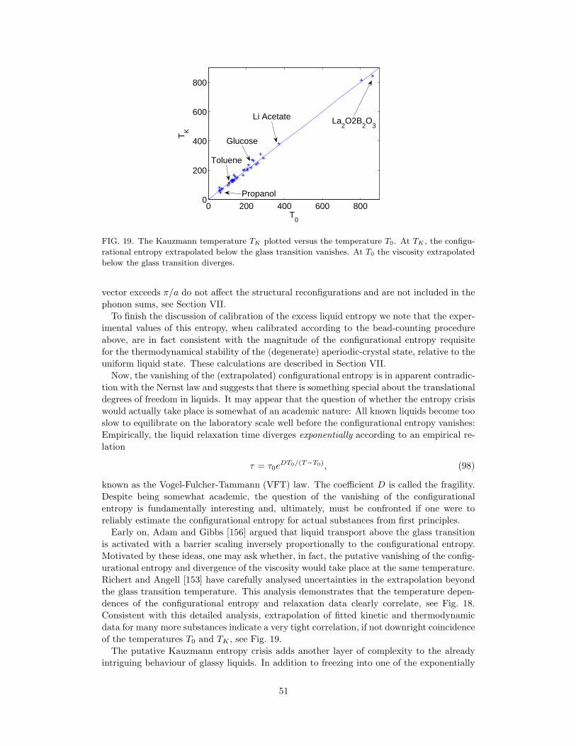
0 200 400 600 8000

200

400

600

800

T0

TK

Propanol

Toluene

Glucose

Li Acetate La2O2B

2O

3

FIG. 19. The Kauzmann temperature TK plotted versus the temperature T0. At TK , the configu-

rational entropy extrapolated below the glass transition vanishes. At T0 the viscosity extrapolated

below the glass transition diverges.

vector exceeds π/a do not affect the structural reconfigurations and are not included in the

phonon sums, see Section VII.

To finish the discussion of calibration of the excess liquid entropy we note that the exper-

imental values of this entropy, when calibrated according to the bead-counting procedure

above, are in fact consistent with the magnitude of the configurational entropy requisite

for the thermodynamical stability of the (degenerate) aperiodic-crystal state, relative to the

uniform liquid state. These calculations are described in Section VII.

Now, the vanishing of the (extrapolated) configurational entropy is in apparent contradic-

tion with the Nernst law and suggests that there is something special about the translational

degrees of freedom in liquids. It may appear that the question of whether the entropy crisis

would actually take place is somewhat of an academic nature: All known liquids become too

slow to equilibrate on the laboratory scale well before the configurational entropy vanishes:

Empirically, the liquid relaxation time diverges exponentially according to an empirical re-

lation

τ = τ0eDT0/(T−T0), (98)

known as the Vogel-Fulcher-Tammann (VFT) law. The coefficient D is called the fragility.

Despite being somewhat academic, the question of the vanishing of the configurational

entropy is fundamentally interesting and, ultimately, must be confronted if one were to

reliably estimate the configurational entropy for actual substances from first principles.

Early on, Adam and Gibbs [156] argued that liquid transport above the glass transition

is activated with a barrier scaling inversely proportionally to the configurational entropy.

Motivated by these ideas, one may ask whether, in fact, the putative vanishing of the config-

urational entropy and divergence of the viscosity would take place at the same temperature.

Richert and Angell [153] have carefully analysed uncertainties in the extrapolation beyond

the glass transition temperature. This analysis demonstrates that the temperature depen-

dences of the configurational entropy and relaxation data clearly correlate, see Fig. 18.

Consistent with this detailed analysis, extrapolation of fitted kinetic and thermodynamic

data for many more substances indicate a very tight correlation, if not downright coincidence

of the temperatures T0 and TK , see Fig. 19.

The putative Kauzmann entropy crisis adds another layer of complexity to the already

intriguing behaviour of glassy liquids. In addition to freezing into one of the exponentially

51

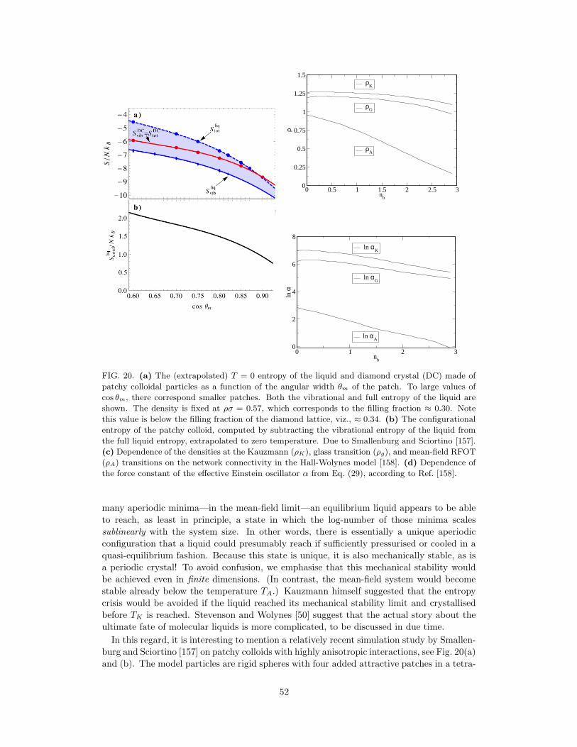
(c)

0 0.5 1 1.5 2 2.5 3n

b

0

0.25

0.5

0.75

1

1.25

1.5

ρ

ρA

ρK

ρG

(d)

0 1 2 3n

b

0

2

4

6

8

ln α

ln αA

ln αK

ln αG

FIG. 20. (a) The (extrapolated) T = 0 entropy of the liquid and diamond crystal (DC) made of

patchy colloidal particles as a function of the angular width θm of the patch. To large values of

cos θm, there correspond smaller patches. Both the vibrational and full entropy of the liquid are

shown. The density is fixed at ρσ = 0.57, which corresponds to the filling fraction ≈ 0.30. Note

this value is below the filling fraction of the diamond lattice, viz., ≈ 0.34. (b) The configurational

entropy of the patchy colloid, computed by subtracting the vibrational entropy of the liquid from

the full liquid entropy, extrapolated to zero temperature. Due to Smallenburg and Sciortino [157].

(c) Dependence of the densities at the Kauzmann (ρK), glass transition (ρg), and mean-field RFOT

(ρA) transitions on the network connectivity in the Hall-Wolynes model [158]. (d) Dependence of

the force constant of the effective Einstein oscillator α from Eq. (29), according to Ref. [158].

many aperiodic minima—in the mean-field limit—an equilibrium liquid appears to be able

to reach, as least in principle, a state in which the log-number of those minima scales

sublinearly with the system size. In other words, there is essentially a unique aperiodic

configuration that a liquid could presumably reach if sufficiently pressurised or cooled in a

quasi-equilibrium fashion. Because this state is unique, it is also mechanically stable, as is

a periodic crystal! To avoid confusion, we emphasise that this mechanical stability would

be achieved even in finite dimensions. (In contrast, the mean-field system would become

stable already below the temperature TA.) Kauzmann himself suggested that the entropy

crisis would be avoided if the liquid reached its mechanical stability limit and crystallised

before TK is reached. Stevenson and Wolynes [50] suggest that the actual story about the

ultimate fate of molecular liquids is more complicated, to be discussed in due time.

In this regard, it is interesting to mention a relatively recent simulation study by Smallen-

burg and Sciortino [157] on patchy colloids with highly anisotropic interactions, see Fig. 20(a)

and (b). The model particles are rigid spheres with four added attractive patches in a tetra-

52

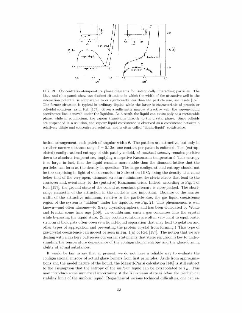
FIG. 21. Concentration-temperature phase diagrams for isotropically interacting particles. The

l.h.s. and r.h.s panels show two distinct situations in which the width of the attractive well in the

interaction potential is comparable to or significantly less than the particle size, see insets [159].

The former situation is typical in ordinary liquids while the latter is characteristic of protein or

colloidal solutions, as in Ref. [157]. Given a sufficiently narrow attractive well, the vapour-liquid

coexistence line is moved under the liquidus. As a result the liquid can exists only as a metastable

phase, while in equilibrium, the vapour transitions directly to the crystal phase. Since colloids

are suspended in a solution, the vapour-liquid coexistence is observed as a coexistence between a

relatively dilute and concentrated solution, and is often called “liquid-liquid” coexistence.

hedral arrangement, each patch of angular width θ. The patches are attractive, but only in

a rather narrow distance range δ = 0.12σ; one contact per patch is enforced. The (extrap-

olated) configurational entropy of this patchy colloid, at constant volume, remains positive

down to absolute temperature, implying a negative Kauzmann temperature! This entropy

is so large, in fact, that the liquid remains more stable than the diamond lattice that the

particles can form at the density in question. The large configurational entropy should not

be too surprising in light of our discussion in Subsection III C; fixing the density at a value

below that of the very open, diamond structure minimises the steric effects that lead to the

crossover and, eventually, to the (putative) Kauzmann crisis. Indeed, according to Fig. 1 of

Ref. [157], the ground state of the colloid at constant pressure is close-packed. The short-

range character of the attraction in the model is also important. Because of the narrow

width of the attractive minimum, relative to the particle size, the gas-liquid coexistence

region of the system is “hidden” under the liquidus, see Fig. 21. This phenomenon is well

known—and often irksome—to X-ray crystallographers, and has been elucidated by Wolde

and Frenkel some time ago [159]. In equilibrium, such a gas condenses into the crystal

while bypassing the liquid state. (Since protein solutions are often very hard to equilibrate,

structural biologists often observe a liquid-liquid separation that may lead to gelation and

other types of aggregation and preventing the protein crystal from forming.) This type of

gas-crystal coexistence can indeed be seen in Fig. 1(a) of Ref. [157]. The notion that we are

dealing with a gas here buttresses our earlier statements that steric repulsion is key to under-

standing the temperature dependence of the configurational entropy and the glass-forming

ability of actual substances.

It would be fair to say that at present, we do not have a reliable way to evaluate the

configurational entropy of actual glass-formers from first principles. Aside from approxima-

tions and the model nature of the liquid, the Mezard-Parisi calculation [148] is still subject

to the assumption that the entropy of the uniform liquid can be extrapolated to TK . This

may introduce some numerical uncertainty, if the Kauzmann state is below the mechanical

stability limit of the uniform liquid. Regardless of various technical difficulties, one can es-

53

tablish useful connections between the bonding patterns in the liquid and its configurational

entropy using a microscopically-motivated model. Hall and Wolynes [158] (HW) used the

self-consistent phonon theory to analyse a hard sphere liquid with randomly added bonds

between particles, so that a particle is bonded on average to nb neighbours. Adding bonds

stabilises contacts energetically but destabilises them entropically. As expected, increasing

the number of bonds dramatically decreases the density ρA at which metastable structure

begin to form while affecting the density ρK of the Kauzmann state only modestly, Fig. 20(c).

The rapid decrease of ρA with the number of rigid bonds is consistent with the results from

Fig. 20(a) and (b) in that increasing directionality makes local bonding patterns more open.

Beyond a certain critical value of bonds a rigid percolation takes place in the network, as

signalled by α−1/2 approaching the particle size a, see Fig. 20(d). The rigidity percolation at

nb ≃ 2.8 is not inconsistent with independent estimates by Thorpe and coworkers [160, 161],

who obtain nb ≃ 2.4. Similarly to the behaviour of the density, adding bonds also affects

the temperature TA much more than TK (both increase), so that the TK/TA ratio decreases.

We shall see in Section VII that the laboratory glass transition occurs at a nearly universal

value of the configurational entropy. This notion, in combination with Eq. (95), implies that

a smaller value of the TK/TA corresponds with the smaller value of the heat capacity jump

at the glass transition ∆cp(Tg). This is qualitatively consistent with observation [61], see

also the inset in Fig. 2.

One should be cautious in interpreting the results in Figs. 20(c) and (d) at values of α

significantly below 102/a2. While these graphs give correct qualitative trends for large to

medium values of α, they could not correspond to an equilibrated liquid for the smallest

values of α, certainly not as small as 1/a2. Indeed, we know that the vibrational displacement

near the mechanical stability limit in directionally bonded materials, such as silicon, is quite

similar in magnitude to that in well-packed materials, see Ref. [105]. In other words, the

model liquid in Figs. 20(c) and (d), if equilibrated, should melt well before the percolation

transition at α ∼ 1/a2 can be reached. Consequently, the liquid is not in the landscape

regime on the low end of the investigated range of α. Conversely, given the apparent

metastability of the network-like states with α ∼ 1/a2, one may infer from the Hall and

Wolynes model that such small values of α could be still be reached, but only off-equilibrium,

i.e., by preparing the glass through rapid quenching or vapour deposition. This notion will

be of use toward the end of the article.

Finally, given the complexity of the interactions in actual materials, it is reasonable to ask

whether one could evaluate the configurational entropy semi-phenomenologically. This way,

those interactions enter in the form of the measured values of materials constants such as

elastic moduli and thermal expansion coefficient, etc. Bevzenko and Lubchenko [154, 155]

have, in part, accomplished this program, to be discussed in Subsection IVD.

We reiterate that it is imperative to recognise that whether or not the configurational

entropy strictly vanishes at some low temperature is not directly relevant to the translational

symmetry breaking that results from the random first order transition. In fact, it is a

common misconception that the existence of the entropy crisis at TK is the essential feature

of the the RFOT. It is not. The only prerequisite for the translational symmetry breaking

at TA is that condition (88) be satisfied. We note also that there is a rigorous sense, in

which the Kauzmann crisis can be defined for a liquid that would not ordinarily have one

in a macroscopic sample. This crisis can be achieved when a finite sample runs out of

configurations, to be discussed in Section VC.

54

C. Qualitative discussion of the transition at TA as a kinetic arrest, by way of

mode-mode coupling. Connection between kinetic and thermodynamic views on the

transition at TA. Short discussion on colloids, binary and metallic mixtures, and ionic

liquids.

Studying the thermodynamic stability of aperiodic solids is certainly not the only way

to approach the problem of the glass transition. Much effort toward understanding the

dramatic slowing-down in supercooled liquids, Fig. 2, was undertaken in the early 1980s

starting from a purely kinetic prospective. This work culminated in the creation of the

mode coupling theory [11, 12, 162] (MCT), which predicts that under certain conditions,

the traditional view of the dynamics of a liquid as being that of a dense gas fails. This

theory builds on early theories of collisional transport [163] and arrives at the conclusion that

already in a uniform liquid, the view of particle transport as a memory-less, Langevin process

eventually becomes internally-inconsistent as the density increases. Given the difficulty of

summing high-order terms in the mode-mode coupling expansion [164], one has to resort to

a mean-field approximation. In this mean-field limit, one discovers that at a high enough

density, a particle’s memory extends indefinitely implying that it no longer moves about but,

instead, forever vibrates around a certain location in space. This behaviour is often called

“caging.” As the cages form, the viscosity diverges, leading to a kinetic catastrophe. These

“cages” turn out to correspond to the metastable structures that emerge during the RFOT.

Indeed, Kirkpatrick and Wolynes [146] have shown that in the mean-field limit, the kinetic

catastrophe of the MCT theory and the RFOT theory are equivalent. In this approach, the

response of the liquid becomes elastic while the equation that self-consistently specifies the

force constant α of the effective Einstein oscillator from Eq. (29) has the same structure as

the DFT-based Eq. (83) for determining α self-consistently:

α =ρ

6

∫dDq

(2π)Dq2c(2)h(q)e−q2/2α, (99)

where the function h is defined in Eq. (68). It turns out that this equation identically

coincides with Eq. (82) in the mean-field limit D → ∞. Indeed, Sq → ρgq in this limit

(since the i = j contribution in Eq. (61) becomes vanishingly small), and so ρhq → Sq (at

q > 0), by Eq. (68). On the other hand, it can be shown [146] that α ∝ D2 as D → ∞, c.f.

Eq. (83); thus S0(q) → S(q). As a result, the kinetic arrest of the MCT exactly coincides

with the inception of the spinodal in F (α), in the mean-field limit. Furthermore, since

the system is equilibrated and must obey detailed balance, it must be true that the set of

states corresponding to the finite value of α at the spinodal are thermodynamically stable.

Otherwise, the system would not have been arrested in a state characterised by a finite α

but, instead, would remain in the uniform state α = 0. In other words, the temperature TAof the RFOT transition strictly coincides with the mean-field spinodal. The above argument

is somewhat subtle because in the strictest mean-field limit, the system could, in principle,

get arrested even in a metastable free energy minimum because the barrier for escape would

be infinite. To make the argument work, we must assume a finite D at the onset, to make the

escape barrier finite and take advantage of detailed balance. At finite D, the temperature

of the spinodal may or may not strictly coincide with the temperature TA at which the

aperiodic-crystal state becomes thermodynamically stable. In the D → ∞ limit, however,

the two temperatures become equal. We shall observe a similar pattern for mean-field spin

models in the next Subsection.

In finite dimensions, the cages do not live forever and eventually disintegrate via ac-

tivated processes, as will be discussed in detail in Section V. Reproducing the activated

processes formally within the the MCT framework appears to be difficult and has not been

accomplished to date, to the author’s knowledge and judgement [165]. Adding activated

55

processes on top of the MCT effects can be done phenomenologically and results in good

fits of temperature dependences of relaxation times [166, 167]. At any rate, the correspon-

dence between the thermodynamics-based RFOT treatment and the MCT survives in finite

dimensions in the sense that the sharp RFOT transition becomes a soft crossover, while the

kinetic catastrophe becomes a gradual rise in viscosity.

Even in its simplest version, the MCT is rather formal in that it discusses correlations

in liquid in terms of coupling between hydrodynamic modes, not molecular motions them-

selves; discussing the technical details of the MCT would be beyond the scope of the article.

Extensive reviews of the MCT can be found elsewhere [168, 169]. Here, instead, we discuss

the kinetic perspective on the RFOT transition in a qualitative, phenomenological fashion,

yet with relatively explicit reference to molecular motions.

Suppose first that particle motions have no memory whatsoever. Under these circum-

stances, we can connect the (thus frequency-independent) self-diffusivity D with the viscos-

ity η via the Stokes-Einstein relation: D = kBT/(6π(a/2)η), where we set the hydrodynamic

radius of the particle at one-half of its volumetric size. By Einstein’s formula, the typical

travelled distance squared goes with time t as⟨r2⟩= 6Dt. Thus the time is takes for a

particle to diffuse its own size is given by:

τex =πηa3

2kBT. (100)

Note that this size represents a secure upper bound on the time it takes for two particles to

exchange identities and thus locally establish configurational equilibrium.

Now suppose that transient structures could, in principle, form in the same system,

whether as a result of a phase transition or not. According to the phenomenological Maxwell

relation (which can be derived constructively, see Section IX), the lifetime of the metastable

structures in such a liquid is intrinsically related to its viscosity and elastic constants:

τ ≃ η

K(101)

The liquid may be regarded as uniform only insofar as we cannot distinguish the particles

by their location. Consequently, when the viscosity is so high that the time a particle “sticks

around” becomes comparable to the lifetime of a transient structure from Eq. (101), we must

conclude that the assumption of the liquid’s uniformity is internally-inconsistent and that

transient structures do, in fact, form. This is the essence of the symmetry breaking that

takes place during the crossover from collisional to activated transport, if expressed in kinetic

terms. Equating the times in Eqs. (100) and (101) yields η = ∞. (There is no η = 0 solution

because because the viscosity of hard spheres is finite and concentration-independent in the

infinite dilution limit.) The η = ∞ solution is internally consistent and corresponds with

the kinetic catastrophe of the MCT, by which the liquid would be completely arrested, in

the mean-field limit.

If one attempts to equate the timescales from Eqs. (100) and (101), with the aim to

estimate the viscosity at which the crossover would actually occur, one quickly discov-

ers a potential issue. These two equations, in combination with the Lindemann criterion,

Ka3 ≃ αa2kBT ≃ 102kBT , would seem to indicate that the exchange time is always longer

than the structural relaxation time τ , whenever the transient structures could exist. (Some

of this excess is intrinsic and some is due to a likely overestimate in Eq. (100).) Yet there

is not necessarily a contradiction here. The condition that τex > τ simply implies that

the emergence of the solid is driven thermodynamically, not kinetically. The finite differ-

ence between τex and τ is inevitable because the kinetic arrest is due to a solidification

transition and is thus a discontinuous transition, as we saw in Section III for the regular

liquid-to-crystal transition and in Subsection IVA for the random-first order transition; this

implies that the viscosities in “pure” uniform liquid and aperiodic crystal should differ by a

56

finite amount. The viscosity of actual substances interpolates between the values given in

Eqs. (100) and (101) and thus changes continuously through the crossover. It seems worth-

while to recall that the finite (and large) value of the inverse Lindemann length squared α,

at a liquid-to-solid transition, is crucial in avoiding the critical point in Fig. 7. Likewise, the

present, crude argument suggests that a continuous kinetic arrest would also be avoided, in

equilibrium, owing to the finite value of α in a solid, be it periodic or aperiodic.

Still, is there a simple way to estimate the viscosity at which the crossover takes place

based on the simplistic reasoning above? To do so, we must use a measure of liquid’s memory

that would be more appropriate at the crossover than that afforded by Eq. (100). The latter

equation clearly does not apply when nearby particles’ movements are tightly correlated,

as in Fig. 17(b). In this regime, the configurational and velocity equilibration processes

are coupled and so one expects the corresponding equilibration times to be mutually tied.

Indeed, the hopping time of vibrational packets is tied to the particle hopping time in that

the latter is an upper bound for the former. On the other hand, the vibrational hopping

time is directly connected with the velocity equilibration. To put this in perspective, the

configurational equilibration is much faster in dilute gases, Fig. 17(a), and vice versa in very

dense liquids or solids, in which collisions are very frequent, Fig. 17(c). In both of these cases

configurational and velocity equilibration processes are decoupled. Velocities equilibrate on

the times comparable to auto-correlation time τauto:

τauto =m

ζ≃ a2ρ

3πη, (102)

where m = ρa3 is the particle mass. Thus, near the crossover, we may associate the

duration of a particle’s memory with the time τauto multiplied by a dimensionless number

C that signifies how many collisions the particle must undergo before the memory of its

location is completely erased: τmemory ∼ Cτauto. Substitution of typical values of the

density, particle size and viscosity in Eq. (102) shows that τauto is very short, shorter than

molecular vibrations. (This is expected as each molecule directly interacts with molecules

from several coordination shells.) The velocity equilibration time should be about two

orders of magnitude greater than τauto, while the configurational equilibration is even slower.

Consequently, the numerical factor C is, very roughly, 103 or greater. We reiterate that

τauto reflects the configurational equilibration only in a narrow density range; note the

inverse scaling of τauto with the viscosity, which is the opposite of what is expected for the

configurational equilibration timescale. Equating τmemory with τ from Eq. (101) yields the

following estimate for the viscosity at the crossover:

η ∼ K(a/cs)C1/2, (103)

where cs is the speed of sound and so a/cs scales with but exceeds a typical vibrational

period of a molecule. Quantitative criteria for crossover will be presented in Section VII,

where we shall see that at Tcr, η ≃ Kτvibr × 103, where τvibr stands for the vibrational

relaxation time.

Although lacking the sophistication of the mode-coupling theory, the qualitative discus-

sion above on the kinetic aspects of the emergence of the landscape makes one realise that

in liquids made of indistinguishable particles, particle collisions and configurational equili-

bration are intrinsically connected: Each particle collides exclusively with particles it must

exchange places with for the liquid to equilibrate. Conversely, the viscous drag on a given

particle is solely due to particles that are identical to that given particle. Colloidal sus-

pensions, among other systems, present a radically different situation. The viscous drag on

a colloidal particle is now largely due to the solvent. Thus by varying the solvent or the

particle size, one can vary the timescale for configurational equilibration at a fixed filling

57

fraction. Alternatively said, the bulk viscosity and structural relaxation are largely decou-

pled in colloidal suspensions. Owing to this decoupling, one can make colloidal particles

arbitrarily sluggish—by increasing their size—without them ever entering the landscape

regime. To quantify these notions, we note the dynamic range accessible to an ordinary,

molecular liquid between the melting point (τ ≃ 10−12) and the crossover to the landscape

regime (τ ≃ 10−9 . . . 10−8) is about 3-4 order of magnitude. By Eq. (100), the exchange

time τex for micron-sized colloidal particles exceeds that for ordinary liquid easily by ten

orders of magnitude, at the same value of the bulk viscosity. This implies that on ordinary

laboratory timescales, such mesoscopic colloids only begin to sample the landscape regime

when their arrest arrest becomes macroscopically apparent.

Likewise, one expects some decoupling between collisions and structural relaxations in

viscous metallic mixtures and heterodisperse mixtures of model particles employed in sim-

ulational studies of slow liquids. In such mixtures, the mole fractions of the ingredients are

comparable and so the degree of decoupling is not nearly as large as in colloids. An alterna-

tive, thermodynamic way to see this is as follows: One often employs eutectic mixtures of

elements to destabilise the crystal state, relative to the liquid, at the same value of viscosity.

By the same token, employing carefully chosen size ratios or molar fractions in mixtures,

one may lower the temperature TA, while not affecting the liquid’s viscosity. Again, this

will lead to an increased dynamic range of the pre-landscape regime. We shall see additional

indications in Subsection XIIA that metallic glasses freeze just below the crossover.

Room temperature ionic liquids represent an intermediate case between colloidal suspen-

sions and metallic mixtures. Like the metals, such liquids are mixtures of molecules that

do not have obvious crystalline ground states. On the other hand, the decoupling between

collisional processes and structural relaxation is significantly greater than in those mixtures.

Because of the very long range of the Coulomb interaction, each molecule directly collides

with a very large number of molecules, not just its nearest neighbours. Indeed, although

the intensity of an individual collision decays as 1/r with distance, the number of molecules

grows as r2 with distance. (The author does not have a simple argument to determine

the collisional range.) We thus conclude ionic liquids are at least as slow and are likely

slower than metallic mixtures and thus are further away from the landscape regime, at a

given value of viscosity. To avoid confusion we note that the above logic does not apply to

traditional ionic liquids such as ZnCl2, since these exhibit a great deal of covalent bonding.

Such liquids are more appropriately though of as dipolar.

D. Connection with spin models

The formal status of the RFOT theory as of the late 80s–mid 90s was somewhat uncertain

for a number of reasons. Given the inherent approximations of the density-functional theory,

the mean-field character of the DFT-MCT connection, and the technical complexity of

the MCT theory [168], many regarded the picture advanced by the RFOT theory of the

structural glass transition as lacking in formal foundation or were unaware of the theory in

the first place. The replica-based calculation of the configurational entropy by Mezard and

Parisi [148] was not available until 1999. Although constructive, that replica calculation,

again, is approximate and relies on the assumption that the mechanical stability limit of

the uniform liquid is not reached above the (putative) temperature TK . On the other hand,

calorimetry data for actual supercooled liquids yield the magnitude of the configurational

entropy requisite for the stability of the aperiodic crystal. Perhaps the most forceful proof

of the activated nature of the liquid transport near the glass transition is that the rate of

the transport is Arrhenius-like below the glass transition, as emphasised in Ref. [170]. Thus,

although the premise of the RFOT theory is clearly consistent with observation—and so are

58

its many predictions!—some of the aspects of the theory itself could be perceived as having

been established only phenomenologically. To fill this perceived formal gap, much technical

effort has been directed at finding solvable models that exhibit features reflecting those of

the structural glass transition.

By the late 1980s, a very interesting disordered model having a glass-like transition had

already been worked out, viz., the mean-field Sherrington-Kirkpatrick (SK) model [171, 172].

This model exhibits a proliferation of metastable minima below a certain temperature,

similar to what happens during the RFOT. The model is an Ising magnet from Eq. (5),

but with randomly distributed couplings Jij . The distribution’s mean is zero. In the mean-

field limit, the couplings should scale not as 1/N , but 1/√N , in contrast with the Ising

ferromagnet. Most commonly, the distribution is assumed to be Gaussian:

p(Jij) =1√

2πJ2/Ne−

J2ij

2J2/N (104)

In an interesting contrast with the regular Ising magnet, we must retain the second order

term in the expression for the molecular field even in the strict mean-field limit:

hmoli =

∑

j

Jijmj −mi

∑

j

βJ2ij(1−m2

j), (105)

c.f. Eq. (38). The reader will recognise β(1 − m2j) at the susceptibility of a spin with

magnetisation mj discussed following Eq. (38). Thus the second order term on the r.h.s.

gives the effective field spin i exerts on itself through interactions with the rest of the spins,

consistent with this term being proportional to mi itself. This term corresponds to the

Onsager cavity field in electrodynamics [173] and turns out to make a finite contribution to

the molecular field in disordered magnets even in the mean-field limit; this contribution is

in fact numerically equal to the first term at the glass transition and thus must be retained

in the free energy expansion [172, 174].

Combined with Eq. (35), which connects the molecular field with local magnetisa-

tion, Eq. (105), forms a closed system of equations, often called the Thouless-Anderson-

Palmer [175] (TAP) equations that can be used, in principle, to determine the equilibrium

magnetisation in the SK magnet. The corresponding free energy reads:

F (mi) = kBT∑

i

(1 +mi

2ln

1 +mi

2+

1−mi

2ln

1−mi

2

)

−∑

i<j

Jijmimj −1

2

∑

ij

βJ2ij(1 −m2

i )(1−m2j), (106)

c.f. Eqs. (6), (7), and (9).

The mean-field system freezes into a “spin-glass” state below a certain, sharply defined

temperature, whereby the number of possible states to freeze into scales with the system

size, in contrast, for instance, with the ordinary Ising magnet, in which the number of such

distinct states is just two. All free energy minima are automatically aperiodic—owing to

the disorder in the couplings—similarly to the liquid below the RFOT. Yet the ergodicity-

breaking transition in the SK model is continuous, in contrast with the liquid. The continuity

of the transition is consistent with the discrete symmetry of the time-inversion symmetry of

the SK hamiltonian, σi ↔ −σi, by which the cubic term and the rest of the odd terms

in the Landau-Ginzburg expansion are expressly forbidden by symmetry.

An equally important piece of distinction between the SK model and the liquid case is that

in the former, the disorder is built-in, or quenched. The multiplicity of the solution is due to

the vast number of configurations available to a magnet with the disordered couplings from

Eq. (104) and a lack of a unique stable state. This type of frustration can be seen already

59

with an Ising antiferromagnet on the 2D triangular lattice: E = −J(σ1σ2 + σ1σ3 + σ2σ3)

with J < 0. The ground state of this system is six-fold degenerate (E = J) and the excited

state is two-fold degenerate (E = −3J). In contrast with the SK model, there is no built-in

disorder in liquids. Instead, the interactions between molecules are perfectly translationally

invariant. The disorder in structural glass is thus entirely self-generated. Although the latter

fact is often cited as a most enigmatic feature of the structural glass transition, it is not

hard to see how frustration could, in principle, arise in 3D liquids. For instance, the Voronoi

cell corresponding to the locally-densest packing in 3D is the regular dodecahedron, which

has a 5-fold symmetry axis and thus does not tile space.

It turns out that the solutions of the free energy (106) have an incredibly rich structure.

The free energy minima are organised into a multi-tiered hierarchy, by which distinct solu-

tions can be classified according to the degree of mutual similarity. It is convenient to think

of these solutions as distinct replicas in the Gibbs ensemble that happened to freeze into dis-

tinct free energy minima, below the glass transition, the same way extensive portions of an

Ising ferromagnet could polarise up or down below the Curie point. For the mean-field SK

model, the similarity of distinct solutions—or replica overlap—is continuously distributed.

This multi-tiered ergodicity breaking was elucidated by Parisi [172], among others, in the

early 1980s and is often called full replica symmetry breaking (RSB).

Already in their 1985 paper, Singh, Stoessel, and Wolynes [143] point out that the free

energy landscape of an aperiodic crystal can bear similarities to the Parisi solution of the

SK model, as the distinct replicas are also aperiodic upon ergodicity breaking. Still, a

meaningful connection between the two systems, if any, was difficult to establish given their

distinct symmetries, even setting aside the lack of quenched disorder in liquids.

Spin models that afford such a connection must not have the time-inversion symmetry of

the Ising model. One such model is the so called p-spin model with an odd p:

E = −∑

i1<i2<...<ip

Ji1i2...ipσi1σi2 . . . σip , (107)

where the couplings are distributed according to

p(Ji1i2...ip) =1√

p!πJ2/Ne−

J2i1i2...ip

p!J2/N . (108)

This model exhibits a one-stage replica symmetry breaking (RSB), for p > 2 [176]. (In the

limit p → ∞, the p-spin model reduces to the so called random energy model (REM) [177,

178] while the calculations simplify significantly.) That all the replica overlaps are the same

implies that all free energy minima are equivalent.

In contrast with the SK model (which corresponds to p = 2), the ergodicity breaking

in the p-spin model is discontinuous for p > 2 [177]. Motivated by this notion and the

mean-field equivalence between the kinetic catastrophe of the MCT and the RFOT [146]

discussed in Subsection IVC, Kirkpatrick and Thirumalai [179, 180] have analysed, upon

Wolynes’s suggestion, a dynamic version of the p-spin model. One way to impart the model

with dynamics is to treat the length of an individual spin as a particle with a finite mass,

whose motion is subject to a soft, bistable potential. Aside from some potential uncertainty

stemming from approximations, these workers discovered that the dynamic p-spin model

undergoes, in mean-field, a kinetic catastrophe at a temperature Tg above the temperature

T ′g at which the replica symmetry is broken.

In 1987, Kirkpatrick and Wolynes [181] (KW) definitively rationalised those intriguing

but enigmatic findings by obtaining a complete solution of the mean-field version of the so

called Potts glass model, using a state-counting strategy employed by Thouless, Anderson,

and Palmer [175]. A formally exact calculation of the free energy of the mean-field Potts

glass had been furnished two years prior, by Gross, Kanter, and Sompolinsky [182]. The

60

Potts model is similar to the SK model, but generally does not exhibit the time-inversion

symmetry and may exhibit a discontinuous ergodicity-breaking transition under certain

circumstances, similarly to the p-spin model. In its most basic form [183], the Potts model is

a generalisation of the Ising model to an energy function of the form E = −∑i<j Jijσ(si, sj),

where the (generally vectorial) spin variables si are allowed to have a chosen, discrete set

of values. The test-function σ(si, sj) = δsi,sj singles out only the configurations in which

the spin variables on sites i and j have the same value. More generally, one may use a test

function that assigns a non-zero weight to si 6= sj configurations also; this weight, however,

must be different from that of the identical configuration, by definition. A common test

function of this kind is simply the scalar product of the vectors, as would be natural in a

Heisenberg model: σ(si, sj) = sisj, however in contrast with Heisenberg-like models, the

spins are not continuous but are allowed to point only in specified directions. Specifically

one often dictates that the spins point toward the vertices of a p-cornered hypertetrahedron

in a flat (p − 1)-dimensional space [184]. Here we set the length of each vector at√p− 1,

by definition. For p = 2, we recover the usual Ising spins; the corresponding test function

sisj is equal to either 1 (si = sj) or −1 (si 6= sj). When p = 3, the spins point toward the

corners of an equilateral triangle with the side√6. The test function can have the value 2

(si = sj) or −1 (si 6= sj). For p = 4, the spins could point toward the corners of the regular

3D tetrahedron, which implies four distinct orientations, and so on. KW considered exactly

this version of the Potts model (for an arbitrary value of p):

E = −∑

i<j

Jij sisj , (109)

where the couplings Jij are random and obey the distribution (104).

For p > 4, the mean-field Potts glass exhibits a discontinuous transition at a temperature

TA, in which an exponential number of solutions emerge, each solution corresponding to a

free energy minimum. The transition exhibits itself as a spinodal at a finite value of the

replica-overlap order parameter, call it q. The free energy just below the spinodal, as a

function of q, looks like the F (α) curve in Fig. 12(a) corresponding to ρσ = 1.05. It turns

out that each individual solution is higher in free energy than the symmetric phase exactly

by TSc, where Sc is the log-number of those solutions times kB . Despite the spectacular

symmetry breaking at TA, the full free energy or entropy of the mean-field Potts glass

does not experience a singularity of any sort. In further contrast with the SK model, the

replica-symmetry breaking at TA is one-stage, not infinite-stage.

Furthermore, the configurational entropy Sc is found to vanish at a finite temperature

TK < TA. Note that in the mean-field model from Eq. (109), the barriers separating the

distinct minima emerging below TA are strictly infinite. This means that the system is al-

ready completely arrested at a temperature TA > TK even as its entropy is finite! KW [181]

pointed out that in finite dimensions, however, the barriers separating the distinct free en-

ergy would be, in fact, finite and so activated transitions between the minima would be

allowed. Accounting for spatial fluctuations already in the long-wavelength approximation,

dictates that there be correlation lengths diverging both at TA, owing to critical-like fluc-

tuations at the spinodal, and diverging at TK , to be discussed in detail in Section V. The

infinite-range correlations at TA would be destroyed by the aforementioned activated tran-

sitions. Complemented by these notions, the exact solution of the mean-field Potts glass

model was important in that it showed that the RFOT-advanced picture of the glass transi-

tion as a kinetic arrest into a degenerate aperiodic crystal is not unique from a purely formal

standpoint. As an added bonus, the Potts glass also exhibits a Kauzmann state.

Because of these apparent similarities between the thermodynamics and kinetics of glassy

liquids and the disordered Potts model, it is still very common to see statements in the

literature that the RFOT picture of the structural glass transition is simply an analogy

61

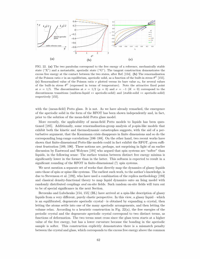
GX

2 2k g /2

dilated aperiodicphase

stable reference state

F

g

k g /2

(a) (b) (c)

FIG. 22. (a) The two parabolas correspond to the free energy of a reference, mechanically stable

state (“X”) and a metastable, aperiodic state (“G”). The tangent construction demonstrates the

excess free energy at the contact between the two states, after Ref. [154]. (b) The renormalisation

of the Poisson ratio ν in an equilibrium, aperiodic solid, as a function of the built-in stress θG [155].

(c) Renormalised value of the Poisson ratio ν plotted versus its bare value ν0, for several values

of the built-in stress θG (expressed in terms of temperature). Note the attractive fixed point

at ν = 1/5. The discontinuities at ν = 1/2 (µ = 0) and ν = −1 (K = 0) correspond to the

discontinuous transitions (uniform-liquid ↔ aperiodic-solid) and (stable-solid ↔ aperiodic-solid)

respectively [155].

with the (mean-field) Potts glass. It is not. As we have already remarked, the emergence

of the aperiodic solid in the form of the RFOT has been shown independently and, in fact,

prior to the solution of the mean-field Potts glass model.

More recently, the applicability of mean-field Potts models to liquids has been ques-

tioned [185]. Additionally, some renormalisation-group analysis of p-spin-like models that

exhibit both the kinetic and thermodynamic catastrophes suggests, with the aid of a per-

turbative argument, that the Kauzmann crisis disappears in finite dimensions and so do the

corresponding long-range correlations [186–188]. On the other hand, two recent works have

shown that finite-dimensional Potts-like models could in fact exhibit the RFOT, given suffi-

cient frustration [189, 190]. These notions are, perhaps, not surprising in light of an earlier

discussion by Eastwood and Wolynes [191] who argued that spin systems are “softer” than

liquids, in the following sense: The surface tension between distinct free energy minima is

significantly lower in the former than in the latter. This softness is expected to result in a

significant rounding of the RFOT in finite-dimensional (!) spin systems.

We next mention a separate set of works that directly map the dynamics of glassy liquids

onto those of spin or spine-like systems. The earliest such work, to the author’s knowledge, is

due to Stevenson et al. [192], who have used a combination of the replica methodology [193]

and classical density-functional theory to map liquid dynamics onto an Ising model with

randomly distributed couplings and on-site fields. Such random on-site fields will turn out

to be of special significance in the next Section.

Bevzenko and Lubchenko [154, 155] (BL) have arrived at a spin-like description of glassy

liquids from a very different, purely elastic perspective. In this view, a glassy liquid—which

is an equilibrated, degenerate aperiodic crystal—is obtained by expanding a crystal, then

letting the atoms settle into one of the many aperiodic arrangements, and then letting the

volume relax. According to a heuristic construction in Fig. 22(a), the free energies of the

periodic crystal and the degenerate aperiodic crystal correspond to two distinct terms, as

functions of deformation. The two terms must cross since the glass term starts at a higher

value of the free energy, but has a lower curvature because the bonding in the aperiodic

sample is softer. This construction explicitly demonstrates there is a mismatch penalty

between the crystal and glass, which corresponds to the excess free energy above the common

62

tangent [194, 195]. To make the glassy state metastable, the aperiodic crystal must be

sufficiently stabilised entropically by the multiplicity of distinct aperiodic arrangements

and by steric repulsion between ill-fitting molecular fragments. The built-in stress pattern

resulting from this repulsion is of shorter wavelength than the regular elastic waves. Thus

in the full free energy of an aperiodic crystal,∫dV uijΛijklukl/2, the full displacement

uij can be profitably presented as a sum of a short-wavelength contribution u>ij and long-

wavelength contribution u<ij . The former and latter take care of the built-in and regular

elastic stress, respectively. The the elastic-moduli tensor Λijkl looks particularly simple for

isotropic elasticity [85]: Λijkl = (K − 2µ/3)δijδkl + 2µ(δikδjl + δilδjk), c. f. Eq. (21). The

model is made non-linear by fixing the magnitude of the local built-in stress; three specific

ways to do so are described in Ref. [155].

The component of the deformation corresponding to the built-in stress violates the so-

called Saint-Venant compatibility condition, whereby a certain combination of the deriva-

tives of the strain (or stress) tensor, called the “incompatibility”, is non-zero:

inc(u>)ij ≡ −ǫiklǫjmn∂u>ln/∂xk∂xm 6= 0. (110)

Setting the incompatibility to zero in the ordinary elasticity theory allows one to obtain the

displacement field u from the tensor of the derivatives uij from Eq. (22) unambiguously; this

way the result is independent of the integration contour [196, 197]. In physical terms the

Saint-Venant compatibility condition guarantees, among other possibilities, that no bonds

are broken. To illustrate this point with a more familiar analogy, one imposes the rotor-

free constraint on the electric field in electrodynamics: ∇ × E = 0 so that the electric

field can be expressed as the gradient of a single-valued, scalar field, viz., the electrostatic

potential. In turn, this implies the energy of an electric charge subject to electric field is a

well defined, single-valued function of the coordinate. Note that the existence of a unique

reference state in continuum mechanics is analogous to stipulating that vacuum be unique

in electrodynamics; it allows one to unambiguously match the particles in the ground and

any excited vibrational state. In contrast, a glassy liquid is a spatial superposition of many

distinct vacua, which thus invalidates the premise of the ordinary elasticity theory. BL [155]

have shown that as long as the degenerate solid is equilibrated, finite-frequency elastic

moduli can still be defined and, in fact, are renormalised versions of the elastic constants in

the individual vibrational “vacua,” as is briefly described below.

Integrating out the regular vibrations, u< in the partition function Tr exp(−β∫dV uijΛijklukl/2),

leads to a Hamiltonian of the type E = −∑i<j siJijsj , c. f. Eq. (109), where the variables

si are now six-component vectors that are allowed to point in any direction and Jij is a

six-by-six matrix. The number six stems from the number of independent entries in the

elastic strain (stress) tensor. (The variables u>ij and s are linearly related.) The coupling Jijis rather complicated and spatially anisotropic, see the explicit expression in Ref. [155], but

scales with the distance and elastic constants as 1/µ(1−ν)r3 (ν is the Poisson ratio). In the

BL approach, there is no built-in disorder. The frustration comes about exclusively because

of the anisotropy of the interaction between local structural excitations. This anisotropy is

similar to, but more complicated than that in the electric dipole-dipole interaction.

In the strict mean-field limit [154], the BL model yields a second order transition be-

tween two regimes corresponding to two types of frozen-in stress, namely, mostly shear and

uniform dilation/contraction respectively. The transition takes place at a specific value of

the Poisson ratio ν = 1/5. BL argued the two regimes typically correspond to strong and

fragile liquids respectively. At the next level of approximation [155], the Onsager cavity

term was included, as in the last term in Eqs. (105) and (106). This results in much richer

thermodynamics compared with the strictest mean-field limit. In addition, the effective

(finite-frequency) elastic constants of the degenerate aperiodic solid can be determined self-

consistently, similarly to how Onsager determined the dielectric constant of a polar liquid

63

based on the molecular dipole moment. The role of the dipole moment is played here by the

magnitude of the built-in stress, which determines the length of the 6-spin. The transition

at ν = 1/5 now becomes an attractive fixed point, see Fig. 22(b) and (c). In addition,

one recovers two more fixed points: one at the uniform liquid (µ/K = 0) and the other at

the infinitely compressible liquid (K = 0). The former transition is self-consistently deter-

mined to be first order, consistent with the RFOT theory. The transition at K = 0—which

corresponds to an infinite compressibility—was speculated to correspond to a mechanical

instability that occurs during pressure-induced amorphisation.

Recently, Yan, During, and Wyart [198] have put forth an elasticity-based model for

glassy-liquid dynamics in which local groups of particles are postulated to possess multiple

alternative states; the associated particle motions are coupled via elastic force fields.

V. QUANTITATIVE THEORY OF ACTIVATED TRANSPORT IN GLASSY LIQ-

UIDS

We begin by remarking that the mean-field limit—which is often a good starting point for

analysing phase transitions—could be somewhat confusing in the case of the random first

order transition. On the one hand, the aperiodic crystal state becomes thermodynamically

stable partially owing to its degeneracy, which in itself is somewhat counter-intuitive since

ordinarily, transitions driven by lowering temperature are accompanied by a decrease in the

(total) entropy. (No discontinuity in the total entropy occurs at the RFOT transition.)

In any event, because the multiplicity of the aperiodic states is a key part of the stabil-

isation, it is essential that the system be able to sample all of those aperiodic structures

without exception. Yet, there are no transitions between the alternative aperiodic minima

in the mean-field limit. This seeming paradox is resolved by noting that the transitions

between the distinct aperiodic are not subject to infinite barriers in finite dimensions. As

already mentioned, Kirkpatrick and Wolynes[181] discussed a mechanism by which individ-

ual aperiodic minima would locally interconvert by means of activated transitions already

in 1987. The driving force for the transitions to occur is precisely the multiplicity of the

distinct aperiodic minima. According to this early argument, the barriers for the activated

transport would scale inversely with the square of the configurational entropy. While the

experimental viscosity curves could be fitted with such a dependence, the inverse linear

scaling matches the empirical Vogel-Fulcher-Tammann law (98) better. In the following, we

discuss α-relaxation in great detail.

Throughout this Section, we will assume the liquid is already in the landscape regime,

i.e., below the temperature Tcr of the crossover between mainly collisional and activated

transport, so that the locally-stable aperiodic structures live significantly longer than the

vibrational relaxation time. In this limit, counting the metastable free energy minima, each

of which corresponds to individual mechanically-metastable structures, becomes unambigu-

ous. Consequently, the configurational entropy, too, is well defined, while the structural

relaxation can be quantitatively described as rare, activated processes, with the help of the

transition state theory [199, 200].

A. Glassy liquid as a mosaic of entropic droplets

We are used to systems whose free energy surface is essentially independent of the system

size: For instance, the free energy surface of a macroscopic Ising ferromagnet below its

Curie point has two distinct free energy minima that can be distinguished by their average

magnetisation, which can be taken to be up or down respectively. If the system is made thrice

bigger, the free energy is simply multiplied by a factor of three; that is, while the number

64

of states within each minimum increases exponentially, the number of minima themselves

remains the same, i.e., two. In contrast, the number of free energy minima in a glassy

liquid scales exponentially with the system size N : escN , as already mentioned. Under

these circumstances, the system will break up into separate, contiguous regions that are

relatively stabilised; the contiguous regions are separated by relatively strained interfaces

characterised by a higher free energy density. To see this, suppose the opposite were true and

the free energy density were uniform throughout. Owing to the multiplicity of distinct free

energy minima, the nucleation rate for another relatively stabilised configuration is finite, as

we will see shortly. As a result, the original configuration will be locally replaced by another

configuration while the boundary of the replaced region will be relatively strained because

of a mismatch between the new structure and its environment. Thus in equilibrium, there

is a steady-state concentration of the strained regions; local reconfigurations take place at a

steady rate between distinct aperiodic structures. The concentration of the strained regions

and the escape rate from the current liquid configuration can be determined self-consistently,

as discussed by Kirkpatrick, Thirumalai, and Wolynes [30], Xia and Wolynes [31], and

Lubchenko and Wolynes [40].

First we provide a somewhat more explicit, “microcanonical” version of that argument,

as detailed recently in Ref. [34]. In a standard fashion, thermodynamic quantities are

Gaussianly distributed in a sufficiently large system. Thus the partition function of a ther-

modynamic system in contact with a thermal bath at temperature T ≡ 1/kBβ and pressure

p can be expressed as a Gaussian integral over the fluctuating value of the Gibbs free energy

G:

Z =

∫dG√2πδG2

e−βG e−(G−G)2/2δG2

. (111)

Here G is the most probable value of the Gibbs free energy and δG =⟨(G−G)2

⟩1/2is the

corresponding standard deviation. It is easy to show [34] that for a region containing N

particles,

δG = N1/2

[kBTK

ρ+ (Kαt − s)2

kBT2

ρcv

]1/2, (112)

where K ≡ −V (∂p/∂V )T is the bulk modulus, and αt ≡ (1/V )(∂V/∂T )p the thermal

expansion coefficient. The quantities cv and s are, respectively, the heat capacity at constant

volume and entropy, both per unit volume. The average particle density ρ can be rewritten

in terms of the volumetric particle size a:

ρ ≡ 1/a3. (113)

There is some freedom in choosing the identity and/or size of the effective particle of the

theory. Often one chooses actual atoms as effective particles so that the particle-particle

interaction can be directly estimated using quantum-chemistry calculations. It is also com-

mon to use a coarse-grained description, in which the particle contains several atoms or

even a non-integer number of atoms. For instance, when treating a molecular substance, it

is often most convenient to use computed from scratch or suitably parametrised potentials,

the most common example of such a parametrised interaction is the Lennard-Jones poten-

tial. (Incidentally, evaluating such intermolecular interactions ab initio is not necessarily

an easy task even for small molecules.) Here we assign the effective particle of the theory

as the bead defined in Eq. (96). This way, we shall be able to take advantage of several

quantitative predictions of the DFT theory, as discussed in Subsection IVB.

Let us now consider a liquid below the crossover to activated transport but above the glass

transition; the liquid is thus equilibrated. Below the crossover, the reconfigurations are rare

65

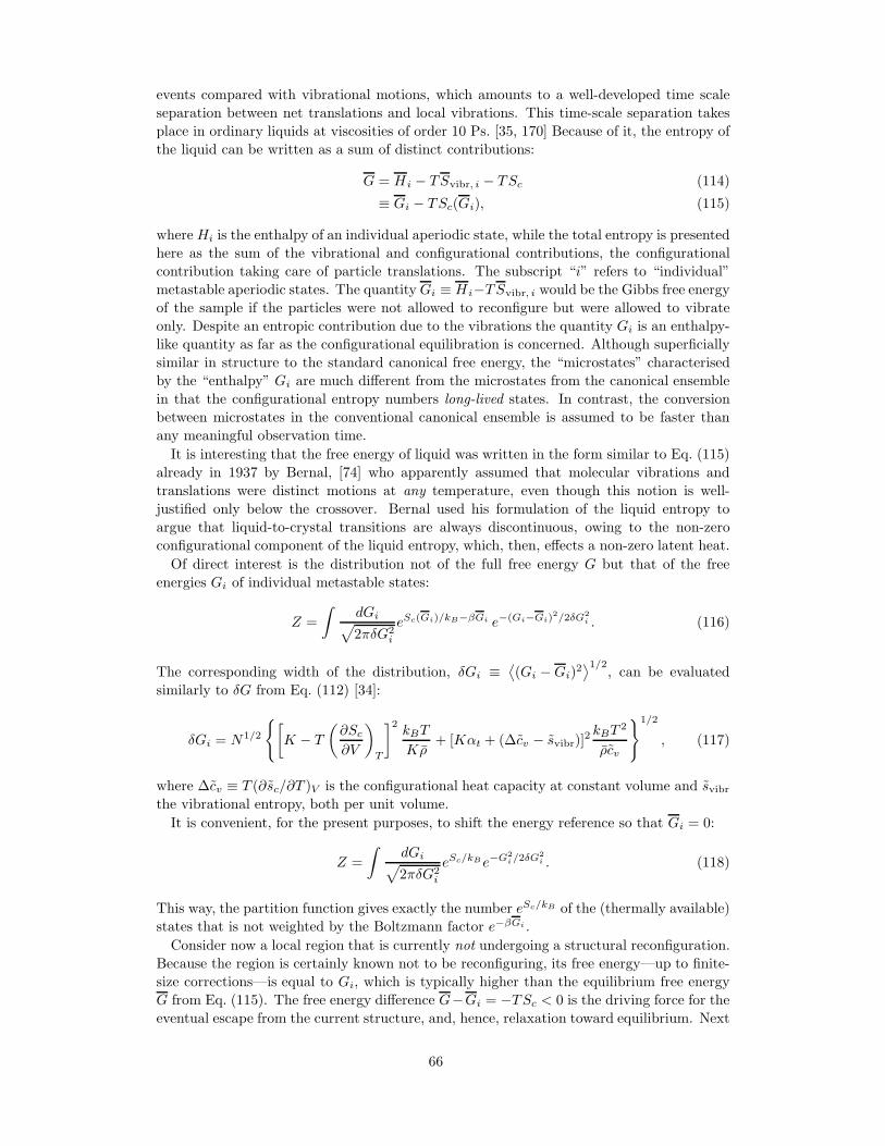
events compared with vibrational motions, which amounts to a well-developed time scale

separation between net translations and local vibrations. This time-scale separation takes

place in ordinary liquids at viscosities of order 10 Ps. [35, 170] Because of it, the entropy of

the liquid can be written as a sum of distinct contributions:

G = Hi − TSvibr, i − TSc (114)

≡ Gi − TSc(Gi), (115)

whereHi is the enthalpy of an individual aperiodic state, while the total entropy is presented

here as the sum of the vibrational and configurational contributions, the configurational

contribution taking care of particle translations. The subscript “i” refers to “individual”

metastable aperiodic states. The quantityGi ≡ Hi−TSvibr, i would be the Gibbs free energy

of the sample if the particles were not allowed to reconfigure but were allowed to vibrate

only. Despite an entropic contribution due to the vibrations the quantity Gi is an enthalpy-

like quantity as far as the configurational equilibration is concerned. Although superficially

similar in structure to the standard canonical free energy, the “microstates” characterised

by the “enthalpy” Gi are much different from the microstates from the canonical ensemble

in that the configurational entropy numbers long-lived states. In contrast, the conversion

between microstates in the conventional canonical ensemble is assumed to be faster than

any meaningful observation time.

It is interesting that the free energy of liquid was written in the form similar to Eq. (115)

already in 1937 by Bernal, [74] who apparently assumed that molecular vibrations and

translations were distinct motions at any temperature, even though this notion is well-

justified only below the crossover. Bernal used his formulation of the liquid entropy to

argue that liquid-to-crystal transitions are always discontinuous, owing to the non-zero

configurational component of the liquid entropy, which, then, effects a non-zero latent heat.

Of direct interest is the distribution not of the full free energy G but that of the free

energies Gi of individual metastable states:

Z =

∫dGi√2πδG2

i

eSc(Gi)/kB−βGi e−(Gi−Gi)2/2δG2

i . (116)

The corresponding width of the distribution, δGi ≡⟨(Gi −Gi)

2⟩1/2

, can be evaluated

similarly to δG from Eq. (112) [34]:

δGi = N1/2

[K − T

(∂Sc

∂V

)

T

]2kBT

Kρ+ [Kαt + (∆cv − svibr)]

2 kBT2

ρcv

1/2

, (117)

where ∆cv ≡ T (∂sc/∂T )V is the configurational heat capacity at constant volume and svibrthe vibrational entropy, both per unit volume.

It is convenient, for the present purposes, to shift the energy reference so that Gi = 0:

Z =

∫dGi√2πδG2

i

eSc/kBe−G2i/2δG

2i . (118)

This way, the partition function gives exactly the number eSc/kB of the (thermally available)

states that is not weighted by the Boltzmann factor e−βGi .

Consider now a local region that is currently not undergoing a structural reconfiguration.

Because the region is certainly known not to be reconfiguring, its free energy—up to finite-

size corrections—is equal to Gi, which is typically higher than the equilibrium free energy

G from Eq. (115). The free energy difference G−Gi = −TSc < 0 is the driving force for the

eventual escape from the current structure, and, hence, relaxation toward equilibrium. Next

66

we estimate the actual rate of escape and the typical region size that will have reconfigured

as a result of the escape event.

We specifically consider escape events that are local. Therefore, the environment of a

chosen compact region is static, up to vibrations. Consider the partition function for a

compact region of size N surrounded by such a static, aperiodic lattice. The vast majority

of the configurations do not fit the region’s boundary as well as the original configuration,

and so there is a free energy penalty Γi > 0 due to the mismatch between the static boundary

and any configuration of the region other than the original configuration. We anticipate that

since local replacement of a structure amounts to a legitimate fluctuation, Γ and δGi should

be intrinsically related, which will indeed turn out to be the case.

In the presence of the mismatch penalty, the density of states can be obtained by replacing

Gi → Gi + Γ under the integral in Eq. (116), where Γ ≡ Γi is the typical value of the

mismatch. The latter generally scales with the region size:

Γ = γNx, (119)

but in a sub-thermodynamic fashion: x < 1, where the coefficient γ(N → ∞) = const.

Thus we obtain for the total number of thermally available states for a region embedded in

a static lattice:

Z =

∫dGi√2πδG2

i

eSc/kB−βΓe−(Gi−Γ)2/2δG2i , (120)

where we set the expectation value of the free energy in the absence of the penalty at zero, as

before. (The expectation value of Gi corresponding to Eq. (120) is not zero at N > 0.) Note

the argument of the first exponential on the r.h.s. is independent of Gi but does depend on

the region size N , and so does the total number of thermally available states Z:

Z(N) = escN/kB−βγNx

, (121)

where sc ≡ Sc/N is the configurational entropy per particle.

Because of the sub-linearN -dependence of the mismatch penalty, the number of thermally

available states Z(N) depends non-monotonically on the region size. For small values of N ,

this number decreases with the region size, which is expected since the region is stable with

respect to weak deformation such as movement of a few particles. At the value N ‡ such

that (∂Z/∂N)N‡ = 0, the number of available stats reaches its smallest value and increases

with N for all N > N ‡. This critical size N ‡:

N ‡ =

(xγ

Tsc

)1/(1−x)

, (122)

corresponds to the least likely size of a rearranging region, and thus corresponds to a bot-

tleneck configuration for the escape event: Indeed, any state at N < N ‡ is less likely than

the initial state and so cannot be a final state upon a reconfiguration; such final state must

thus be at N > N ‡. On the other hand, to move any number of particles N in excess of

N ‡, one must have moved N ‡ particles as an intermediate step.

The size N∗ > N ‡ such that

Z(N∗) = 1 (123)

is special in that the region of this size is guaranteed to have a thermally available configu-

ration, distinct from the original one, even though the boundary is fixed. By construction,

this configuration is mechanically (meta)stable. This implies that a region of size N∗:

N∗ =

(γ

Tsc

)1/(1−x)

, (124)

67

i

N=5

G

Local Library N=5Initial ConfigurationGlobal Library Local Library N=7

N=7

FIG. 23. Illustration of the library construction of aperiodic states [40]. On the left, we start out

with some metastable structure. The density of the horizontal bars reflects the increase of the

density of states (DoS) eSc(Gi)/kB with Gi. This DoS is distinct from the probability distribution

in Eq. (120), which also includes the Boltzmann factor e−βGi . In the centre and right panels,

5 and 7 particles have been moved. The density of states pertaining to the corresponding local

regions are much lower than the global density of states. In addition, the majority of the thus

obtained configurations are higher in free energy than the original configuration, owing to the

mismatch with the environment. As the region size grows, the distribution of free energies Gi of

individual structures is determined by a competition between a depletion due to the mismatch and

an entropically-driven increase in the DoS. For a large enough N = N∗, there will be a configuration

whose free energy Gi is comparable to that of the original structure.

can always reconfigure. What happens physically is that the centre of the free energy distri-

bution from Eq. (120) moves to the right with N according to γNx because the mismatch

typically increases with the interface area. This alone would lead to a depletion of states

that are degenerate with the original state, which is typically at Gi = 0. Yet as N increases,

the free energy distribution also grows in terms of the overall area, height, and, importantly,

width, as more states become available. For a sufficiently large size N∗, the distribution is so

broad that the region is guaranteed to sample a state at Gi = 0 even though the distribution

centre is shifted to the right by Γ. One may say that in such a state, a negative fluctuation

in the free energy exactly compensates the mismatch penalty. For this to be typically true,

we must have

Γ(N) = δGi(N) at N = N∗, (125)

where we have emphasised that both Γ and δG depend on N .

Finally note that the physical extent ξ of the reconfiguring region:

(ξ

a

)3

≡ 4π

3

(R∗

a

)3

≡ N∗ (126)

yields the volumetric cooperativity length for the reconfigurations.

The above notions can be discussed explicitly in terms of particle movements, within the

library construction of aperiodic states [40], graphically summarised in Fig. 23. We start

out with the original state, which is some state from the full set of states available to the

68

system. We then draw a surface encompassing a compact region containing N particles and

consider all possible configurations of the particles inside while the environment is static

up to local elastic deformations, i.e., vibration. Most of the resulting configurations are,

of course, very high in energy because of steric repulsion between the particles comprising

the region itself and between the particles on the opposite sides of the the boundary. Only

few configurations will contribute appreciably to the actual ensemble of states, and even

those are offset upwards, free energy-wise, by the mismatch penalty. As the chosen region is

made progressively bigger, three things happen at the same time: (a) the mismatch penalty

typically increases as γNx; (b) the log-number of available states first decreases but then

begins to increase, asymptotically as ∝ N ; and (c) the spectrum of states becomes broader,

the width going as ∝√N . Think of (a) as a density of states eS(Gi)/kB that moves up

according to γNx with the region size (see Fig. 23), thus leading to a “depletion” of the

density of states at low Gi. Items (b) and (c), on the other hand, mean the density of states

increases in magnitude roughly as escN−Γ−(Gi−Γ)2/2δG2

, at fixedGi (δG ∝√N and Γ ∝ Nx).

For a large enough N , this growth of the density of states, at fixed Gi, dominates the

depletion due to the mismatch penalty and so the free energy of the substituted configuration

eventually stops growing and begins to decrease with the region size N , after the latter

reaches a certain critical value N ‡. Eventually, at size N∗, one will typically find an available

state that is mechanically stable.

The discussion of the statistical notions embodied in Eqs. (119)-(124) in terms of particle

motions helps one to recognise that the full set of configurations in some range [0, Nmax] can

be sorted out into (overlapping) subsets according to the following protocol: (a) within each

subset, every region size is represented at least once and (b) two configurations characterised

by sizes N and (N +1) differ by the motion of exactly one particle. The subsets thus corre-

spond to dynamically-connected paths, along each of which particles join the reconfiguring

region one at a time. Along each of the dynamically connected paths, one could thus think

of the reconfiguration as a droplet growth. A certain path will dominate the ensemble of the

paths given a particular final configuration. This dominating path is the one that maximises

the number of states Z(N) from Eq. (121) (including all intermediate values of N , of course).

This is entirely analogous to the Second Law, whereby the equilibrium configurations are

those the maximise the density of states (subject to appropriate constraints).

One may take the notion of the dynamic connectivity even further by noting that consec-

utive movements must be directly adjacent in space because the nucleus grows is a sequence

of individual bead movements. Such movements—whether belonging to the same or distinct

reconfigurations—interact, the interaction scaling with distance r as 1/r3, similarly to the

electric dipole-dipole interaction [154]. The nucleus growth in Eq. (128) differs, for instance,

from nucleation of liquid inside vapour in that in the latter, gas particles can join the nucleus

from any side, while in the former, consecutive bead movements are relatively likely to be

neighbours in physical space, in which case the movements form a contiguous chain. Now,

how extensive are these individual bead displacements? At the crossover, the individual

free energy minima are marginally stable with respect to transitions between each other

and with respect to the decay into the uniform liquid state α = 0. Xia and Wolynes [31]

thus concluded that the vibrational displacements within individual free energy minima

should be numerically close to the value prescribed by the Lindemann criterion of melting,

i.e., one-tenth of the volumetric particle size or so:

dL ≃ a/10. (127)

Conversely, displacements just beyond this length will result in a transition between distinct

free energy minima. An important corollary of the result in Eq. (127) is that individual bead

motions are nearly harmonic, that is, no bonds are broken. The total combination of the

individual moves is, of course, an anharmonic process since both the initial and final state are

69

metastable and are thus separated by a barrier. A well-known example of such anharmonic

processes consisting of individual harmonic motions are rotations of rigid SiO4/2 tetrahedra

in silica [201]. Another explicit example will be considered in Subsection XIIB, in which a

covalent bond does not break but, instead, becomes a weaker, secondary bond. The energy

cost of an individual bead movement is modest.

One may question whether the most likely bottle-neck configuration in the set of all

dynamically connected paths leading to the final state at N∗ is, in fact, as likely as what

is prescribed by Z(N ‡) with Z(N) from Eq. (121). The answer is yes because sampling

of all possible shapes and locations for a region of size N is implied in the summation in

Eq. (120). By backtracking individual dynamically-connected trajectories from N = N∗

to N = 0, we can determine the precise reconfigured region that produces the most likely

bottle-neck configuration with probability Z(N ‡).

Now, for region sizes in excess of N∗, the number Z(N) of available states exceeds one,

implying that, for instance, two distinct metastable configurations are available to a region

of size N such that Z(N) = 2. According to the above discussion, the trajectories leading to

these two states are generally distinct, though the probabilities of the respective bottle-neck

configurations and the corresponding critical sizes N ‡ should be comparable.

Structural reconfiguration can be equally well discussed not in a microcanonical-like fash-

ion, through the number of states Z(N), but, instead, in terms of the corresponding free

energy F (N) = −kBT lnZ(N), as was originally done by Kirkpatrick, Thirumalai, and

Wolynes [30]. This yields the following activation profile for the reconfiguration:

F (N) = Γ− TscN ≡ γNx − TscN, (128)

Since we are considering all possible configurations for escape, subject to the appropriate

Boltzmann weight, this amounts to locally replacing the original configuration encompassing

N particles by the equilibrated liquid while the particles in the surrounding are denied any

motion other than vibration. Upon the replacement, the local bulk free energy is typically

lowered by G−Gi = −TscN , hence the driving term −TscN in Eq. (128).

The equilibrated liquid is a Boltzmann-weighted average of alternative, metastable ape-

riodic structures that are mutually distinct and are also generally distinct from the initial

configuration. Another way of saying two structures are distinct is that the particles be-

longing to the structures inside and outside do not fit as snugly—at the interface between

the structures—as they do within the respective basis structures. This is quite analogous to

the mismatch between two distinct crystalline polymorphs in contact, such as must occur

during a first order transition between the polymorphs. In contrast with a polymorphic

transition, the scaling of the mismatch penalty with the area of the interface will turn out

to be somewhat complicated, viz, the exponent x need not be (D − 1)/D.

Combining the free energy view with the notion of dynamically connected trajectories,

due to the library construction, we conclude that the activation profile in Eq. (128) is also a

nucleation profile. Naturally, the bottle-neck configuration corresponding to N = N ‡ from

Eq. (122) thus corresponds to the critical nucleus size. The corresponding barrier is equal

to

F ‡ ≡ F (N ‡) = γ

(xγ

Tsc

)x/(1−x)

(1− x) = γ(1− x) (N ‡)x. (129)

This directly shows that the escape rate from a specific aperiodic state is indeed finite. Note

also that the cooperativity size is always equal to the critical size N ‡ times an x-dependent

numerical coefficient:

N∗ = N ‡ x−1/(1−x) > N ‡. (130)

70

Yet there is more to the activation profile in Eq. (128). In ordinary theories of nucleation,

the nucleus continues to grow indefinitely once it exceeds the critical size, unless it collides

with other growing nuclei, as happens during crystallisation, or, for instance, when the

supply of the contents for the minority phase runs out, as happens when a fog forms. This

essentially unrestricted growth takes place because this way, the system can minimise its

free energy by fully converting to the minority phase. Such a view is adequate when there

are only two free energy minima to speak of and the system converts between those two

minima.

However in the presence of an exponentially large number of free energy minima, we

must think about the meaning of the F (N) curve more carefully. We must recognise that

both the initial and final state for the escape event are individual aperiodic states that

are, on average, equally likely. In fact, because we have chosen Gi = 0 as our free energy

reference, F (N) gives exactly the log-number (times −kBT ) of thermally available states to

the selected region. As a result, that the free energy F (N) reaches its initial value of zero

indicates that a mechanically metastable state has become available to escape to. One is

accustomed to situations in which the initial and final state for a barrier-crossing event are

minima of the free energy, which does not seem to be the case in the above argument. There

is no paradox here, however. The quantity F (N) is not the actual free energy of the system.

Instead, by construction, it is the free energy under the constraint that the outside of the

selected compact region is not able to relax in the usual matter, but, instead, is forced to be

in a specific, metastable aperiodic minimum. The monotonic decrease of F (N) at N = N∗

is trivial in that it simply says the surrounding of the droplet will eventually proceed to

reconfigure again and again, as it should in equilibrium. As we have already emphasised,

the state to which the initial configuration has escaped is perfectly metastable.

We now shift our attention to the energy. Suppose the liquid is composed of particles

that are not completely rigid, and so the mismatch penalty has an energetic component.

Furthermore, it is instructive to suppose that the penalty is mostly energetic, which is

probably the case for covalently bonded substances such as silica or the chalcogenides. [29]

At a first glance, the energy of the system appears to grow with each nucleation event, since

the driving force in Eq. (128) is exclusively entropic, at equilibrium. Such unfettered energy

growth is, of course, impossible in equilibrium. On the contrary, the configurations before

and after a reconfiguration are typical and the energy must be conserved, on average. The

energy change following a transition must be within the typical fluctuation range, which

reflects the heat capacity CV at constant volume and the bulk modulus K: [55]

δE = kBCvT2 − V [T (∂p/∂T )V − p]2T/K1/2. (131)

Note both CV and V pertain to a single cooperative region. The conservation of energy, on

average, means that since one new interface appears following an escape event, an equivalent

of one interface must have been subsumed during an event, as emphasised in Ref. [54].

We thus conclude that the equilibrium concentration of the interface configurations is

given by 1/ξ3 with ξ from Eq. (126), and so a glassy liquid is a mosaic of aperiodic struc-

tures, [31] each of which is characterised by a relatively low free energy density, while the

interfaces separating the mosaic cells are relatively stressed regions characterised by excess

free energy density due to the mismatch between stabilised regions. This stress pattern is

not static, but relaxes at a steady pace so that a region of size ξ reconfigures once per time

τ , on average:

τ = τ0eF ‡/kBT , (132)

where the pre-exponent τ0 corresponds to the vibrational relaxation time. It is the same

vibrational-hopping time we encountered in Subsection IVC. Since the nucleation is driven

71

by the multiplicity of distinct aperiodic configurations, i.e., by the configurational entropy,

a glassy liquid may be said to be a mosaic of entropic droplets [31].

Note that the total free energy stored in the strained regions corresponding to the domain

walls is equal to Γ(N/N∗) = TscN , i.e. the enthalpy difference between the liquid and

the corresponding crystal at the temperature in question, up to possible differences in the

vibrational entropy between the crystal and an individual aperiodic structure.

Note that every metastable configuration—which contains both the relatively relaxed and

strained regions—is a true free energy minimum of the liquid. This is in contrast with the

mean-field view we usually take of macroscopic phase coexistence, by which extensive por-

tions of the sample are occupied by structures corresponding to true minima of the bulk free

energy density, such as the two minima in Fig. 8. Appropriately, the physical boundary be-

tween those macroscopic regions then corresponds to the saddle-point in the bulk free energy

in Fig. 8 and to a saddle point solution of the free energy of a nucleating droplet. Thus only

in the mean-field limit do the relatively stabilised regions in glassy liquids correspond with

true free energy minima. (Their multiplicity is still given by the configurational entropy!)

In finite dimensions, there is a steady-state, uniform density of both relatively stabilised

and relatively strained regions, whose spatial density can be determined self-consistently, as

explained above.

We finish this Subsection by describing a somewhat distinct way to think about the mosaic,

due to Bouchaud and Biroli [202]. In this view, the ensemble of all states of a compact

region of size ξ consists of a contribution from the current state and contributions of the

full, exponentially large set of alternative structures. As in the library construction, the

surrounding of the chosen region is constrained to be static up to vibrational displacement.

What sets apart the current state from all the alternative states is that it fits the environment

better. The partition function for the region thus goes roughly as:

ZBB ≃ e−β(−γNx) + eNsc/kB . (133)

The mismatch free energy γNx scales with the region sizeN sublinearly, x < 1, while the log-

number of alternative states scales linearly. Thus the stability of sufficiently small regions—

smaller than ξ—can be understood thermodynamically in a straightforward manner: The

energetic advantage of being in the current state, due to the matching boundary, outweighs

the multiplicity of poorer matching, higher energy states. This is not unlike the stability

of a crystal relative to the liquid below freezing. Indeed, at liquid-crystal equilibrium, the

partition function of the system can be written as Z = e−β(−∆H) + e∆S/kB , where ∆H > 0

and ∆S > 0 are the fusion enthalpy and entropy respectively.

The just listed aspects of the Bouchaud-Biroli picture are essentially equivalent to the li-

brary construction, and, in particular, with regard to the entropic nature of the driving force

for the activated transport. In contrast with the KTW [30] and library construction [40],

however, the BB scenario is agnostic as to the concrete mechanism of mutual reconfiguration

between alternative aperiodic states, other that the reconfigurations must be rare, activated

events. In the absence of such a concrete mechanism, BB posited a generic scaling relation

between the cooperativity size and the relaxation barrier that is similar to that transpiring

from Eqs. (129) and (130). In this view, a region larger than the size N∗ can still reconfigure

via a single activated event but would do so typically more slowly than the region of size

N∗. Combining this notion with the lower bound on the cooperativity size obtained above

one concludes that the cooperativity size is in fact N∗ and one does not face the subtlety

stemming from the downhill decrease of the free energy profile F (N) from Eq. (128). The

present picture contrasts with the Bouchaud-Biroli approach in that it specifically prescribes

that the activated reconfigurations take place through a process akin to nucleation.

Now, according to Eqs. (122)-(126), we need to evaluate the exponent x and the coefficient

γ for the mismatch penalty, to estimate the escape rate and the cooperativity size for the

72

activated reconfigurations, to which we proceed next.

B. Mismatch Penalty between Dissimilar Aperiodic Structures: Renormalisation

of the surface tension coefficient

The mismatch penalty between two ill-fitting structures can be evaluated with the help

of the free energy functional. This evaluation is particularly straightforward in the long

wavelength approximation represented by the Landau-Ginzburg functional from Eq. (3),

which is often called the Cahn-Hiilliard [203] functional in the context of nucleation. Further

simplification is achieved when the nucleus is very large [194, 195], provided that the interface

remains of finite width. Hereby the interface can be effectively regarded as flat while the

total mismatch penalty scales asymptotically linearly with the interface area. Under these

circumstances, the characteristics of the interface are determined by two parameters. One

parameter is the coefficient κ at the square gradient term in Eq. (3), the other is the barrier

height g‡ in the bulk free energy density V (φ), see Fig. 8. The expressions for the width l

and the surface tension coefficient σ read

l ∼√κ/g‡, (134)

and

σ ∼√κg‡ ∼ g‡l, (135)

respectively; both equalities are within factors of order one, which depend on the specific

form of the free energy functional. The total mismatch penalty goes as 4πr2g‡l, consistentwith simple dimensional analysis. Roughly speaking, the excess free energy g‡l per unit

area reflects the free energy penalty due to unsatisfied bonds at the interface, see also

Eq. (12). In the case of rigid particles, bonds are not defined, but analogous expressions

involving the direct correlation function instead of the pair-interaction potential can be

written, as in Eq. (26).One recognises that the interface width l reflects the interaction (or

direct correlation) range—according to Eqs. (12) and (26)—and thus is not directly tied to

the molecular size, even though the two are often numerically similar.

Because the states on both sides of our interface are aperiodic, the degree of mismatch is

distributed [204, 205]. Thus in some places the two structures may fit quite well and so the

scaling of the surface energy term Γ from Eq. (128) with the droplet size N may be weaker

than the N (D−1)/D scaling expected for interfaces separating periodic or spatially uniform

phases. The mechanism of this partial lowering of the mismatch penalty is as follows: The

number of distinct aperiodic structures available to a sufficiently large region, we remind,

scales exponentially with the region size. The free energies Gi of individual structures from

Eq. (115) are distributed; they are equal on average but differ by a finite amount for any

specific pair of aperiodic states. Fluctuations of extensive quantities scale with√N as

functions of size N . [55] (The size N at which the√N scaling sets in can be rather small in

the absence of long-range correlations, such as those typical of a critical point.) Thus the

free energy difference between the configurations outside and inside scales as√N , for two

regions of the same size N , and could be of either sign. Suppose now, for concreteness, that

the configuration on the outer side of the domain wall happens to be lower in free energy

than the adjacent region on the inside. Imagine distorting the domain wall so as to replace

a small portion of the inside configuration by that from the outside. It turns out the free

energy stabilisation due to the replacement outweighs the destabilisation due to the now

increased area of the interface, as we shall see shortly.

Before we proceed with this analysis, it is instructive to discuss why such surface renormal-

isation and the consequent stabilisation would not take place during regular discontinuous

73

transitions when one phase characterised by a single free energy minimum nucleates within

another phase also characterised by a single free energy minimum. After all, both phases

represent superpositions of microstates whose energies are also distributed. Furthermore,

there seems to be a direct correspondence between, say, the regular canonical ensemble and

the situation described in Eq. (115). Hereby, the free energies Gi in Eq. (115) seem to

correspond to the energies of the microstates, while the configurational entropy Sc seems

to correspond to the full entropy in the canonical ensemble. One difference between the

situation in Eq. (115) and the canonical ensemble is that in the latter, transitions between

the microstates within individual phases occur on times much shorter than the observation

time or mutual nucleation and nucleus growth of the two phases. As a result, the energies of

the phases on the opposite sides of the interface are always equal to their average values. In

contrast, the distinct aperiodic states from Eq. (115) are long-lived. In fact, the fastest way

to inter-convert between those states is via creation of the very interface we are discussing!

In the canonical ensemble analogy, this would correspond to having individual microstates

on the opposite sides of the interface as opposed to ensembles resulting from averaging

over all microstates (with corresponding Boltzmann weights). Conversely, the situation in

Eq. (115) would be analogous to the canonical ensemble only at sufficiently long times that

much exceed the nucleation time from Eq. (132). Note that at such long times, we have

identical, equilibrated liquid on both sides and so there is no surface tension in the first

place.

Now, the situation where the system can reside in long-lived states whose free energies

are distributed in a Gaussian fashion can be equivalently thought of as a perfectly ergodic,

equilibrated system in the presence of a static, externally-imposed random field whose fluc-

tuations scale in the Gaussian fashion. In the absence of this additional random field, the

mismatch penalty between such two regular phases would be perfectly uniform along an

interface with spatially uniform curvature. The simplest system one can think of, in which

this situation is realised, is the random field Ising model:

H = −J∑

i<j

σiσj −∑

i

hiσi, σi = ±1, (136)

where J > 0 while the Zeeman splittings hi’s are random, Gaussianly distributed variables.

In the Hamiltonian above, if one were to impose a smooth interface between two macroscopic

domains with spins up and down, the domain wall would distort some to optimise the

Zeeman energy. However, the amount of distortion is also subject to the tension of the

interface between the spin-up and spin-down domains. The overall lowering of the free

energy, due to the interface distortion, corresponds to the optimal compromise between

these two competing factors. Likewise, a smooth interface between two distinct aperiodic

states will distort to optimise with respect to local bulk free energy, which is distributed. The

energy compensation will scale, again, as the square root of the variation of the volume swept

by the interface during the distortion. The final shape of the interface will be determined

by the competition between this stabilisation and the cost of increasing the area of the

interface.

The mapping between the random field Ising model (RFIM) and large scale fluctuations of

the interface between aperiodic liquid structures was exploited by Kirkpatrick, Thirumalai,

and Wolynes (KTW) [30], who used Villain’s argument [206] for the renormalisation of the

surface in RFIM to deduce how the droplet interface tension scales asymptotically with the

droplet size. The mapping relies crucially on the condition that the undistorted interface

must not be too thick, as it would be near a critical point. This assumption turns out to be

correct since the width of the undistorted interface is on the order of the molecular length

a [32].

Let us now review a variation on the KTW-Villain argument concerning the surface ten-

sion renormalisation. This argument produces the scaling relation we seek for the mismatch

74

penalty but some of its steps are only accurate up to factors of order one, and so the latter

will be dropped in the calculation. All lengthscales will be expressed in terms of the molec-

ular length a, which simply sets the units of length. Now, consider two dissimilar aperiodic

states in contact, and assume we have already coarse-grained over all length-scales less than

r, while explicitly forbidding interface fluctuations on greater lengthscales. The interface is

thus taut. Further, consider spatial variations in the shape of the interface on lengthscales

limited to a narrow interval [r, r(1 + ∆)]. The dimensionless increment

∆ = d ln r (137)

is the increment of the running argument for our real-space coarse-graining transformation

r → r(1 + ∆). (Ultimately, r will be set at the droplet radius). We may assume, without

loss of generality, that the mismatch penalty may be written in the following form, in D

spatial dimensions:

Γ = σ(r)rD−1 , (138)

The quantity σ(r) may be thought of as a renormalised surface tension coefficient, where

the amount of renormalisation generally depends on the wavelength, which is distributed in

the (narrow) range between r and r(1+∆). Our task is to determine under which condition

such renormalisation takes place, if any.

To do this, let us deform the interface so as to create a bump of (small) height ζ and

lateral extent r, see sketch in Fig. 24. Because the interface is taut, the area will increase

quadratically with ζ. The resulting increase in the interface area will incur a free energy

cost

δFs ∼ σ(r)rD−1(ζ/r)2∆, (139)

when ζ ≪ r. It will turn out to be instructive to use a more general form

δFs ∼ σ(r)rD−1(ζ/r)z∆. (140)

This generalised form is convenient because (a) rough interfaces may exhibit a z other than

2, (b) the scaling of the interface tension with r will turn out be independent of z at the

end of the calculation. Thus the obtained σ vs. r scaling can be argued to still apply even

to situations when ζ/r is not necessarily small. (Which it will not be!) Now, as already

mentioned, one can always flip a region (of size N) at the interface so a to lower its bulk

free energy by ∼ h√N . The resulting bulk free energy gain is thus:

δFb ∼ −h√N∆ ∼ −h(rD−1ζ)1/2∆, (141)

where the constant h is straightforward to estimate in light of our earlier discussion that

the bulk stabilisation above is the result of fluctuations of the Gibbs free energy. Thus,

h ∼ δGi/√N, (142)

with δGi from Eq. (117). Properly, we should have written h2 = 2(δGi)2/N in Eq. (142)

because the bulk free energy stabilisation is a difference between two random Gaussian

variables, whose distribution widths are δGi each, but we have agreed to drop factors of

order one in the derivation, see also below.

Next we find the value of ζ that optimises the total free energy stabilisation: ∂(δFs +

δFb)/∂ζ = 0, which yields:

ζ ∼ (h/σ)2/(2z−1)r(2z−D+1)/(2z−1). (143)

75

∆

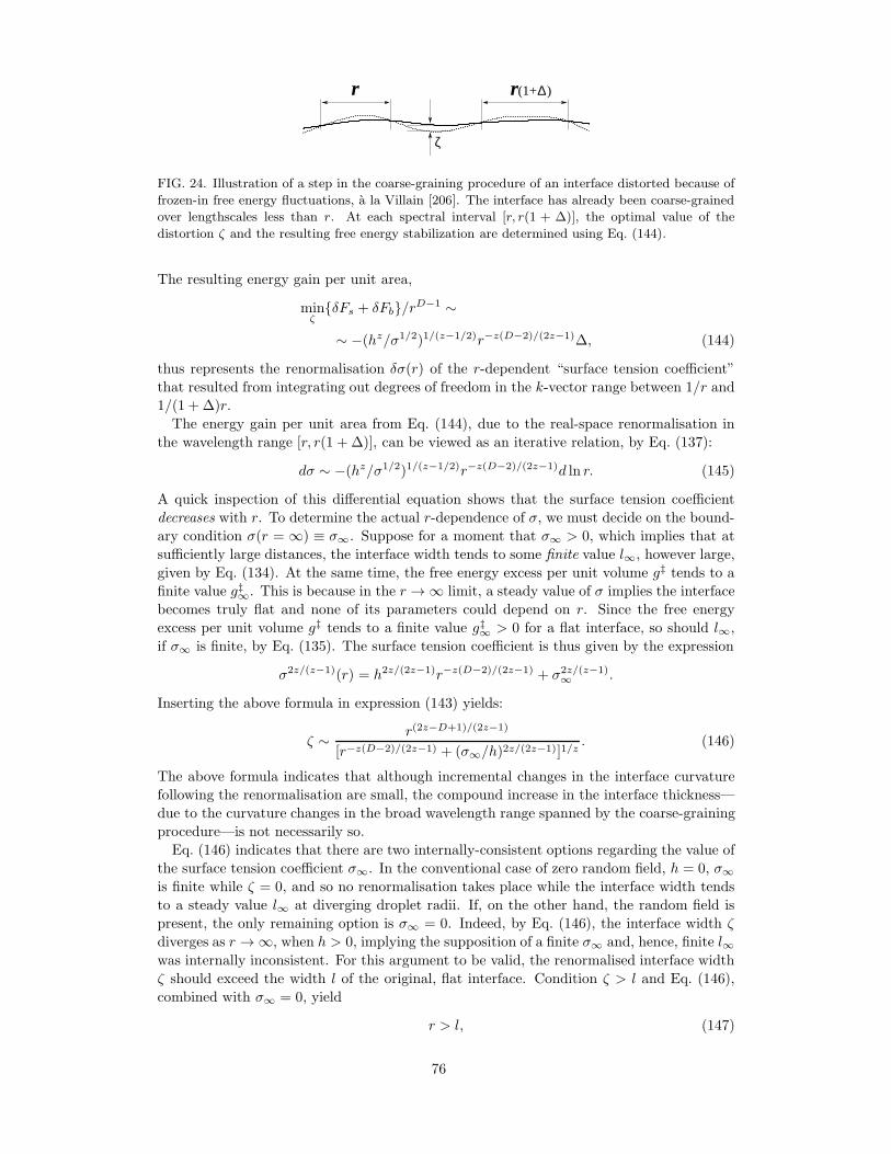
ζ

r r(1+ )

FIG. 24. Illustration of a step in the coarse-graining procedure of an interface distorted because of

frozen-in free energy fluctuations, a la Villain [206]. The interface has already been coarse-grained

over lengthscales less than r. At each spectral interval [r, r(1 + ∆)], the optimal value of the

distortion ζ and the resulting free energy stabilization are determined using Eq. (144).

The resulting energy gain per unit area,

minζ

δFs + δFb/rD−1 ∼

∼ −(hz/σ1/2)1/(z−1/2)r−z(D−2)/(2z−1)∆, (144)

thus represents the renormalisation δσ(r) of the r-dependent “surface tension coefficient”

that resulted from integrating out degrees of freedom in the k-vector range between 1/r and

1/(1 + ∆)r.

The energy gain per unit area from Eq. (144), due to the real-space renormalisation in

the wavelength range [r, r(1 + ∆)], can be viewed as an iterative relation, by Eq. (137):

dσ ∼ −(hz/σ1/2)1/(z−1/2)r−z(D−2)/(2z−1)d ln r. (145)

A quick inspection of this differential equation shows that the surface tension coefficient

decreases with r. To determine the actual r-dependence of σ, we must decide on the bound-

ary condition σ(r = ∞) ≡ σ∞. Suppose for a moment that σ∞ > 0, which implies that at

sufficiently large distances, the interface width tends to some finite value l∞, however large,

given by Eq. (134). At the same time, the free energy excess per unit volume g‡ tends to a

finite value g‡∞. This is because in the r → ∞ limit, a steady value of σ implies the interface

becomes truly flat and none of its parameters could depend on r. Since the free energy

excess per unit volume g‡ tends to a finite value g‡∞ > 0 for a flat interface, so should l∞,

if σ∞ is finite, by Eq. (135). The surface tension coefficient is thus given by the expression

σ2z/(z−1)(r) = h2z/(2z−1)r−z(D−2)/(2z−1) + σ2z/(z−1)∞ .

Inserting the above formula in expression (143) yields:

ζ ∼ r(2z−D+1)/(2z−1)

[r−z(D−2)/(2z−1) + (σ∞/h)2z/(2z−1)]1/z. (146)

The above formula indicates that although incremental changes in the interface curvature

following the renormalisation are small, the compound increase in the interface thickness—

due to the curvature changes in the broad wavelength range spanned by the coarse-graining

procedure—is not necessarily so.

Eq. (146) indicates that there are two internally-consistent options regarding the value of

the surface tension coefficient σ∞. In the conventional case of zero random field, h = 0, σ∞is finite while ζ = 0, and so no renormalisation takes place while the interface width tends

to a steady value l∞ at diverging droplet radii. If, on the other hand, the random field is

present, the only remaining option is σ∞ = 0. Indeed, by Eq. (146), the interface width ζ

diverges as r → ∞, when h > 0, implying the supposition of a finite σ∞ and, hence, finite l∞was internally inconsistent. For this argument to be valid, the renormalised interface width

ζ should exceed the width l of the original, flat interface. Condition ζ > l and Eq. (146),

combined with σ∞ = 0, yield

r > l, (147)

76

which happens to coincide with the criterion of validity of the thin interface approximation.

Note that in their analysis of barrier softening effects near the crossover, Lubchenko and

Wolynes [35] self-consistently arrived at a similar criterion, viz., r > a, for when interface

tension renormalisation would take place.

It follows that an arbitrarily weak, but finite random field h makes an interface with a

sufficiently low curvature unstable with respect to distortion and lowering of the effective

surface tension:

σ(r) ∼ h

aD−1(r/a)−(D−2)/2, (148)

independent of z, apart from a proportionality constant of order one, giving us confidence

in the result even when the undulation size ζ is not very small. Notice we have restored the

units of length for clarity.

Eq. (148) yields that the renormalised mismatch energy Γ from Eq. (138) scales with the

droplet size N in a way that is independent of the space dimensionality, namely√N :

Γ ∼ σ(r)rD−1 ∼ h(r/a)D/2 ∼ h√N, (149)

which is ultimately the consequence of the Gaussian distribution of the free energy. Because

of the lack of a fixed length scale in the problem—other than the trivial molecular size a,

which sets the units—it should not be surprising that the interface width ζ scales with the

radius r itself:

ζ ∼ r, (150)

again independent of z. The numerical constant in the above equation is of order one, as is

easily checked, and so ζ/r is not small generally.

The large effective interface width can be thought of as a result of the distortion of the

original thin interface where the extent of the distortion is not determined by a fixed length,

but the curvature of the interface itself. In other words, this interface is a fractal object.

Because of this fractality, the structure at the interface is not possible to characterise as

either of the aperiodic structures on the opposite sides of the original flat interface before

the renormalisation. We could thus informally think of this fractal interface as the original

thin interface wetted [31] by other structures that interpolate, in an optimal way, between

the two original aperiodic structures. While we are not aware of direct molecular studies

with regard to the fractality of cooperative regions in non-polymeric liquids, such studies of

polymer melts do suggest the mobile regions have a fractal character [207].

According to Eq. (149), the scaling exponent x is equal to 1/2. Thus the matching

condition in Eq. (125) is valid at all values ofN and so we arrive at a central result [30, 31, 34]:

Γ = γ√N. (151)

where

γ = δGi/√N = const. (152)

The resulting free energy nucleation profile:

F (N) = γ√N − TscN, (153)

is shown in Fig. 25(a).

In retrospect, the square-root scaling in Eq. (151) is natural: In view of Eq. (119), the

(Gi − Γ)2/2δG2i term under the second exponential in Eq. (120) scales asymptotically with

N according to N2x−1, see also Ref. [208]. For any x other than 1/2, this would result in an

77

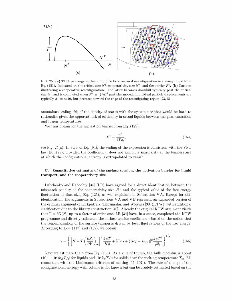
F

N

F(N )

N

N*

(a)

N*dL

Nξ

(b)

FIG. 25. (a) The free energy nucleation profile for structural reconfiguration in a glassy liquid from

Eq. (153). Indicated are the critical size N‡, cooperativity size N∗, and the barrier F ‡. (b) Cartoon

illustrating a cooperative reconfiguration. The latter becomes downhill typically past the critical

size N‡ and is completed when N∗ ≡ (ξ/a)3 particles moved. Individual particle displacements are

typically dL ≃ a/10, but decrease toward the edge of the reconfiguring region [23, 51].

anomalous scaling [26] of the density of states with the system size that would be hard to

rationalise given the apparent lack of criticality in actual liquids between the glass transition

and fusion temperatures.

We thus obtain for the nucleation barrier from Eq. (129):

F ‡ =γ2

4Tsc, (154)

see Fig. 25(a). In view of Eq. (94), the scaling of the expression is consistent with the VFT

law, Eq. (98), provided the coefficient γ does not exhibit a singularity at the temperature

at which the configurational entropy is extrapolated to vanish.

C. Quantitative estimates of the surface tension, the activation barrier for liquid

transport, and the cooperativity size

Lubchenko and Rabochiy [34] (LR) have argued for a direct identification between the

mismatch penalty at the cooperativity size N∗ and the typical value of the free energy

fluctuation at that size, Eq. (125), as was explained in Subsection VA. Except for this

identification, the arguments in Subsections VA and VB represent an expanded version of

the original argument of Kirkpatrick, Thirumalai, and Wolynes [30] (KTW), with additional

clarification due to the library construction [40]. Already the original KTW argument yields

that Γ = δG(N) up to a factor of order one. LR [34] have, in a sense, completed the KTW

programme and directly estimated the surface tension coefficient γ based on the notion that

the renormalisation of the surface tension is driven by local fluctuations of the free energy.

According to Eqs. (117) and (152), we obtain:

γ =

[K − T

(∂Sc

∂V

)

T

]2kBT

Kρ+ [Kαt + (∆cv − svibr)]

2 kBT2

ρcv

1/2

. (155)

Next we estimate the γ from Eq. (155). As a rule of thumb, the bulk modulus is about

(101− 102)kBT/ρ for liquids and 102kBT/ρ for solids near the melting temperature Tm [67]

(consistent with the Lindemann criterion of melting [65, 107]). The rate of change of the

configurational entropy with volume is not known but can be crudely estimated based on the

78

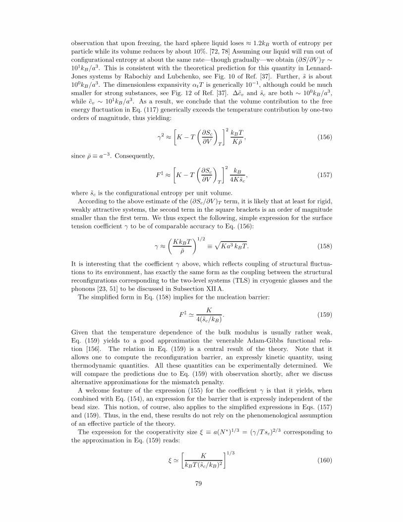
observation that upon freezing, the hard sphere liquid loses ≈ 1.2kB worth of entropy per

particle while its volume reduces by about 10%. [72, 78] Assuming our liquid will run out of

configurational entropy at about the same rate—though gradually—we obtain (∂S/∂V )T ∼101kB/a

3. This is consistent with the theoretical prediction for this quantity in Lennard-

Jones systems by Rabochiy and Lubchenko, see Fig. 10 of Ref. [37]. Further, s is about

100kB/a3. The dimensionless expansivity αtT is generically 10−1, although could be much

smaller for strong substances, see Fig. 12 of Ref. [37]. ∆cv and sc are both ∼ 100kB/a3,

while cv ∼ 101kB/a3. As a result, we conclude that the volume contribution to the free

energy fluctuation in Eq. (117) generically exceeds the temperature contribution by one-two

orders of magnitude, thus yielding:

γ2 ≈[K − T

(∂Sc

∂V

)

T

]2kBT

Kρ, (156)

since ρ ≡ a−3. Consequently,

F ‡ ≈[K − T

(∂Sc

∂V

)

T

]2kB

4Ksc, (157)

where sc is the configurational entropy per unit volume.

According to the above estimate of the (∂Sc/∂V )T term, it is likely that at least for rigid,

weakly attractive systems, the second term in the square brackets is an order of magnitude

smaller than the first term. We thus expect the following, simple expression for the surface

tension coefficient γ to be of comparable accuracy to Eq. (156):

γ ≈(KkBT

ρ

)1/2

≡√Ka3 kBT . (158)

It is interesting that the coefficient γ above, which reflects coupling of structural fluctua-

tions to its environment, has exactly the same form as the coupling between the structural

reconfigurations corresponding to the two-level systems (TLS) in cryogenic glasses and the

phonons [23, 51] to be discussed in Subsection XIIA.

The simplified form in Eq. (158) implies for the nucleation barrier:

F ‡ ≃ K

4(sc/kB). (159)

Given that the temperature dependence of the bulk modulus is usually rather weak,

Eq. (159) yields to a good approximation the venerable Adam-Gibbs functional rela-

tion [156]. The relation in Eq. (159) is a central result of the theory. Note that it

allows one to compute the reconfiguration barrier, an expressly kinetic quantity, using

thermodynamic quantities. All these quantities can be experimentally determined. We

will compare the predictions due to Eq. (159) with observation shortly, after we discuss

alternative approximations for the mismatch penalty.

A welcome feature of the expression (155) for the coefficient γ is that it yields, when

combined with Eq. (154), an expression for the barrier that is expressly independent of the

bead size. This notion, of course, also applies to the simplified expressions in Eqs. (157)

and (159). Thus, in the end, these results do not rely on the phenomenological assumption

of an effective particle of the theory.

The expression for the cooperativity size ξ ≡ a(N∗)1/3 = (γ/Tsc)2/3 corresponding to

the approximation in Eq. (159) reads:

ξ ≃[

K

kBT (sc/kB)2

]1/3(160)

79

This formula can be rewritten in a convenient form for the cooperativity volume:

ξ3 ≡ N∗a3 = [4 ln(τ/τ0)]2 kBT

K. (161)

Given the rule of thumb that Ka3/kBT ≃ 102, we obtain that at the glass transition, where

ln(τ/τ0) ≈ 35, the cooperativity size is about 102 beads.

Note that neither of the expressions (157), (159) and (160) depends explicitly on the

molecular length scale a ≡ ρ−1/3. In this sense, these expressions are truly scale-free, con-

sistent with the scale-free character of the ordinary, gaussian fluctuations of thermodynamic

quantities. In contrast, the presence of anomalous scaling generally requires that a molec-

ular length scale be present explicitly [26], see also our earlier comment on the square-root

scaling of the mismatch penalty following Eq. (152). The simple result in Eq. (159) has

another notable feature with regard to scaling [34]. It is the only expression of units en-

ergy one could write down using the bulk modulus and the configurational entropy per unit

volume that does not involve temperature. The proportionality of the barrier to the bulk

modulus is a direct indication of the activated nature of the reconfigurations and implies

that the latter must involve bond stretching.

On the other hand, the configurational entropy in the denominator of Eq. (159) reflects

the progressively smaller number of degrees of freedom available to the liquid at lower tem-

peratures (or higher pressures), which thus leads to fewer possibilities to find an alternative

metastable state and a downhill trajectory to reach that state. This is also reflected in the

entropy dependence of the cooperativity length (160): Given the decreasing log-number of

states per unit volume, at lower temperatures, searching through larger regions is required

to find an alternative structural state.

We have already remarked that the square-root scaling of the mismatch penalty is natural

in the absence of criticality because otherwise the free energy would exhibit anomalous

scaling. The square root scaling is due to the Gaussian nature of the fluctuations that

lead to reconfigurations. But why would generic Gaussian fluctuations lead to non-generic

consequences in glassy liquids? The answers lies in the exponential multiplicity of distinct

free energy minima, which introduces new physics in the problem. Following Bouchaud

and Biroli [202], one may think of the long-lived structures as residing in traps that are

enthalpically stabilised relatively to a state in which such traps are only marginally stable

and in which the liquid rearrangements are thus nearly barrierless. This is similar to the

way a crystal in equilibrium with the corresponding liquid can be thought of as a trap

which is lower in enthalpy than the liquid whereby the enthalpic stabilisation due to the

trapping exactly matches the excess liquid entropy times temperature. A similar situation

takes place when a folded protein molecule is in equilibrium with the unfolded chain. Now,

in the presence of a thermodynamically large number of free energy minima, fluctuations

become possible that enthalpically stabilise local regions. The extent of such a special

fluctuation is not arbitrary; its value can be determined self-consistently, in equilibrium,

by matching the (enthalpic) stabilisation due to the fluctuation with the log-multiplicity of

the minima: δGi = Tsc. (To avoid confusion we repeat that the quantity Gi is enthalpy-

like with respect to the configurational degrees of freedom even though it includes entropic

contributions due to vibrations.) Combined with Eq. (152), this yields γ√N∗ = TscN

∗ at

the cooperativity size. No such local trapping is possible when the multiplicity of the minima

is sub-thermodynamic, i.e., when the system is not in the landscape regime. Indeed, this

equation has no solutions, if the log-number of the minima per particle, sc/kB, is identically

set to zero.

This simple result above would be modified in the presence of long-range correlations

such as those near critical points. Yet we have seen that a liquid-to-solid is an avoided

critical point, the degree of separation from criticality reflected in the substantial value of

the force constant of the effective Einstein oscillator α ∼ Ka/kBT ∼ 102/a2, see Eq. (30).

80

Consistent with this notion, the energetics of structural fluctuations are dominated by the

elastic modulus K, see Eqs. (152) and (158), which greatly exceeds the thermal energy

scale kBT/a3. On the other hand, the appearance of the bulk modulus in Eqs. (158) and

(159) is consistent with our earlier notion that no bonds are broken during the structural

reconfigurations.

It is quite possible that in addition to the trivial, Gaussian fluctuations, smaller-scale

fluctuations of distinct nature are also present. For instance, in their recent replica-based

work, Biroli and Cammarota [209] argue there is a “wandering” length scale associated with

fluctuations of the domain wall shape. This length diverges with lowering the temperature

as 1/s1/2c , as opposed to the stronger divergence ξ ∝ 1/s

2/3c from Eq. (160). Such wandering

could be important at higher temperatures, see Section VII.

The preceding discussion pertains exclusively to glassy liquids. It seems instructive to

consider now an apparent counterexample in the form of an amorphous silicon film. When

quenched sufficiently below the glass transition, a glassy liquid forms an amorphous solid.

Just below the glass transition, the glass can still undergo activated reconfigurations of the

type discussed above, but somewhat modified for the initial state being off-equilibrium;

this will be explained in detail in Subsection VIII A. In contrast, silicon is a very poor

glass-former and so its amorphous form must be prepared by means other than quenching,

for instance, by sputtering on a cold substrate. The poor glass-forming ability of silicon is

consistent with our earlier notion that this substance would not crossover into the landscape

regime; instead it crystallises at relatively low densities such that the steric effects are

still relatively unimportant. Still, according to the present discussion it would seem that

amorphous silicon could undergo structural reconfigurations similar of glassy liquids. After

all, silicon films are aperiodic and low-density thus resulting in vast structural degeneracy.

Indeed, the density of such films is at least 10% less than that of the crystal (p. 1004

of Ref. [210]) let alone the liquid. The liquid excess entropy of equilibrated silicon at this

density much exceeds the configurational entropy below the crossover. To be fair, the

landscape of amorphous silicon is largely energetic, not free-energetic; it is well above the

equilibrium energy at the ambient conditions. But this would not seem to make a huge

difference as far as the barriers between the (metastable) energy minima are concerned. Are

these barriers given by an expression of the type in Eq. (159)? First note that in contrast

with glassy liquids, we may no longer use the expression (155) for the mismatch penalty,

since it was derived assuming equilibrium. Furthermore, since the enthalpy of the film

is dominated by the (highly anisotropic) bonding, it is likely that silicon will rearrange by

breaking bonds; the mismatch penalty will thus reflect the corresponding, higher energy scale.

Additional complications arise from the fact that the films do not correspond to a structure

that was equilibrated at any temperature, see Subsection VIII A. Another indicator that

reconfigurations in amorphous silicon films must involve bond breaking is that such films

host bulk quantities of dangling bonds [210], something of relevance in the context of photo-

voltaic applications of the material. In addition to being efficient scatterers of charge carriers,

the dangling bonds are directly witnessed by a substantial ESR signal; in contrast, a proper

bond is formed by a filled molecular orbital. Reconfigurations, if any, clearly fail to “heal”

such dangling bonds in silicon films. Conversely, glasses made by quenching equilibrated

liquids do not exhibit significant numbers of dangling bonds. Thus based on the high energy

cost of rearrangements and the relationship between the barrier and the cooperativity size

from Eq. (129), we tentatively conclude that the cooperativity size in amorphous silicon

likely exceeds that in glasses made by quenching. We will continue this discussion later on.

Now, the linear scaling of the activation barrier in Eq. (159) with the elastic modulus

hearkens back to earlier, enthalpy based approaches to activated dynamics by Hall and

Wolynes [211] and the so called “shoving model” [212]. Some of the particular realisations

of the shoving model [213, 214] posit that the dominant contribution to the temperature

81

dependence of the barrier is due to the temperature dependence of the elastic moduli. More

specifically, the shoving model postulates that the barrier goes as KVc, where Vc stands

for the volume of a rearranging region which is prescribed by system specific interactions

and is temperature independent. In contrast, the RFOT theory demonstrates that the

configurational entropy is the leading contributor to the T -dependence of the barrier, and

increasingly so at lower temperatures [33], see also below. Appropriately, the cooperativity

volume must increase with decreasing entropy, see Eq. (160).

In view of the intrinsic relation between the elastic constants and the localisation pa-

rameter α [42], Eq. (30), the above argument connects the mismatch penalty γ with the

“localisation” of the particles upon the crossover at Tcr. Yet this connection is only indirect.

The original calculation of γ, due to Xia and Wolynes [31], explicitly connects the mismatch

penalty to the formation of the metastable structures in which the particles vibrate around

steady-state average locations. It is this original calculation, dating from 2000, that en-

abled the majority of quantitative predictions by the RFOT theory. This calculation will

be reviewed next.

The activation profile from Eq. (153) can be rewritten in terms of the droplet radius

(assuming a spherical geometry) as:

F (r) = 4πr2σ0(a/r)1/2 − (4π/3)(r/a)3Tsc, (162)

using the following connection between the particle number contained within the droplet

and the droplet radius:

N ≡ 4π

3(r/a)3. (163)

This yields for the reconfiguration barrier:

F ‡

kBT=

3π(σ0a2/kBT )

2

sc/kB. (164)

and the cooperativity length:

ξ/a = (4π/3)1/3(3σ0a

2

Tsc

)2/3

. (165)

To estimate the surface tension coefficient σ0, which corresponds to the mismatch penalty

at the molecular scale: σ = σ(r = a), we begin with the density profile from Eq. (29)

in which the lattice sites ri are arranged in an aperiodic fashion, as in Subsection IVA.

This profile is an excellent approximation to the actual density distribution, even though

it ignores the possibility that the force constant α of the effective Einstein oscillator may

be somewhat spatially distributed. The aperiodic crystal forms despite the one-particle

entropic cost ∆floc > 0 of the localisation of a particle around a certain location in space.

The reason is that this localisation also offers a free energy gain, due to multi-particle effects,

as the collisions are now less frequent, as we have already discussed following Eq. (54). In

the presence of chemical interactions, there is also an enthalpy gain due to bond formation.

Both gains contribute to the free energy in formally equivalent ways (through the direct

correlation function) and thus can be formally termed “bonding;” denote the corresponding

free energy difference ∆fbond < 0. Additional stabilisation comes from the multiplicity of

aperiodic states: −Tsc < 0.

The mismatch between two degenerate states can be thought of as partial lack of

“bonds”—a half or so—for a particle at the interface, leading to about (−∆fbond)/2

per particle in missing free energy. Estimating the bonding free energy appears gener-

ally difficult, however obtaining a formal lower bound on −∆fbond is not: Below the

82

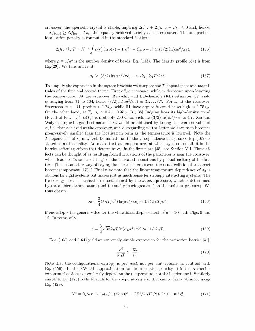
crossover, the aperiodic crystal is stable, implying ∆floc + ∆fbond − Tsc ≤ 0 and, hence,

−∆fbond ≥ ∆floc − Tsc, the equality achieved strictly at the crossover. The one-particle

localisation penalty is computed in the standard fashion:

∆floc/kBT = N−1

∫ρ(r) [ln ρ(r)− 1] d3r − (ln ρ− 1) ≃ (3/2) ln(αa2/πe), (166)

where ρ ≡ 1/a3 is the number density of beads, Eq. (113). The density profile ρ(r) is from

Eq.(29). We thus arrive at

σ0 ≥ [(3/2) ln(αa2/πe)− sc/kB] kBT/2a2. (167)

To simplify the expression in the square brackets we compare the T -dependences and magni-

tudes of the first and second terms: First off, α increases, while sc decreases upon lowering

the temperature. At the crossover, Rabochiy and Lubchenko’s (RL) estimates [37] yield

α ranging from 71 to 104, hence (3/2) ln(αa2/πe) ≃ 3.2 . . . 3.7. For sc at the crossover,

Stevenson et al. [41] predict ≈ 1.2kB, while RL have argued it could be as high as 1.75kB.

On the other hand, at Tg, sc ≃ 0.8 . . . 0.9kB. [31, 35] Judging from its high-density trend

(Fig. 3 of Ref. [37]), α(Tg) is probably 200 or so, yielding (3/2) ln(αa2/πe) ≃ 4.7. Xia and

Wolynes argued a good estimate for σ0 would be obtained by taking the smallest value of

α, i.e. that achieved at the crossover, and disregarding sc; the latter we have seen becomes

progressively smaller than the localisation term as the temperature is lowered. Note the

T -dependence of sc may well be immaterial to the T -dependence of σ0, since Eq. (167) is

stated as an inequality. Note also that at temperatures at which sc is not small, it is the

barrier softening effects that determine σ0, in the first place [35], see Section VII. These ef-

fects can be thought of as resulting from fluctuations of the parameter α near the crossover,

which leads to “short-circuiting” of the activated transitions by partial melting of the lat-

tice. (This is another way of saying that near the crossover, the usual collisional transport

becomes important [170].) Finally we note that the linear temperature dependence of σ0 is

obvious for rigid systems but makes just as much sense for strongly interacting systems: The

free energy cost of localisation is determined by the kinetic pressure, which is determined

by the ambient temperature (and is usually much greater than the ambient pressure). We

thus obtain

σ0 =3

4(kBT/a

2) ln(αa2/πe) ≈ 1.85 kBT/a2, (168)

if one adopts the generic value for the vibrational displacement, a2α = 100, c.f. Figs. 9 and

12. In terms of γ:

γ =3

2

√3πkBT ln(αLa

2/πe) ≈ 11.3 kBT. (169)

Eqs. (168) and (164) yield an extremely simple expression for the activation barrier [31]:

F ‡

kBT≃ 32.

sc. (170)

Note that the configurational entropy is per bead, not per unit volume, in contrast with

Eq. (159). In the XW [31] approximation for the mismatch penalty, it is the Arrhenius

exponent that does not explicitly depend on the temperature, not the barrier itself. Similarly

simple to Eq. (170) is the formula for the cooperativity size that can be easily obtained using

Eq. (129):

N∗ ≡ (ξ/a)3 ≃ [ln(τ/τ0)/2.83]2 = [(F ‡/kBT )/2.83]

2 ≈ 130/s2c. (171)

83

0.02 0.05 0.1 0.2 0.5 1

10

15

20

30

50

70

100

150

D

0.02 0.05 0.1 0.2 0.5 1

10

15

20

30

50

70

100

150

KCaNO3

glycerol

Zn Cl2

Ge O2

1/ΔCp (K Mol/J)

m-fluorotoluene

o-terphenylKBiCl

*

(a)

0 25 50 75 100m, theory

0

25

50

75

100

125

150

m, m

easu

red

(b)

FIG. 26. Tests of the Xia-Wolynes relation between the barrier for activated transport and the

configurational entropy per bead (170), from Ref. [31]. (a) The relation (172) between the fragility

from (98) and heat capacity jump per bead, is shown with the solid line. The experimental points

are indicated with symbols. The bead count is determined based on chemical considerations. (b)

The straight line corresponds to the Lubchenko-Wolynes [35] relation (174). The experimental

points, shown with the symbols, were compiled by Stevenson and Wolynes [36]. The bead count is

from Eq. (96). No adjustable constants used in either estimate.

Notwithstanding its approximate nature, the argument leading to Eq. (170) makes explicit

use of the physical picture emerging from the RFOT theory in that it directly traces the

origin of the mismatch penalty to the confinement of the particle following the breaking of

the translational symmetry and the general inability of arbitrary aperiodic arrays of such

localised particles to mutually fit. The approximations boil down to a few simple notions:

On the one hand, we have neglected the configurational entropy, which would be strictly

valid only at TK . On the other hand, we have replaced the inequality in Eq. (167) by the

equality, which would be strictly valid at the crossover temperature Tcr. In addition, there is

an uncertainty in the value of α, which, however, is only logarithmic. As a result, the energy

scale in Eq. (168) could, in principle, vary between kBTcr and kBTK , but not much beyond

that. In any event, the temperature dependence of the numerator in Eq. (170) is much

weaker than that of the configurational entropy. According to this equation, the barrier

should, in fact, diverge if the configurational entropy vanishes. This prediction is, arguably,

the most important result of the RFOT theory. It shows that the kinetic catastrophe

and the thermodynamic singularity, which are the landmarks of the glass transition, are

intrinsically related. The kinetic catastrophe manifests itself through the rapid growth of

the viscosity above the glass transition that implies the viscosity would diverge at some

putative temperature T0, Fig. 2, if one had the ability to equilibrate the liquid on the

correspondingly increasing time scales. The thermodynamic singularity is the vanishing

of the configurational entropy at the (putative) Kauzmann temperature TK , as in Fig. 18.

According to Eq. (170), the temperatures T0 and TK must coincide, which is consistent with

available extrapolations of kinetic and calorimetric data, see Fig. 19.

In addition to prescribing that T0 = TK , Eq. (170) predicts that the rate of change of the

barrier with temperature is determined by the rate of change of the configurational entropy.

Both of these rates have a clear physical meaning and value in themselves: The slope of

the T -dependence of the log-viscosity actually reflects the width of the temperature window

in which the supercooled liquid will be in a certain viscosity interval of convenience for

processing. The broader the window, the less need for maintaining a constant temperature

during the processing. The corresponding materials are called “long” glasses. Conversely

84

substances with a narrow processing window are called “short” glasses. In a more modern

parlance, due to Angell [61], the former and latter and often called “strong” and “fragile,”

see Fig. 2. Accordingly, the coefficient D from the VFT law in Eq. (98) is called the fragility.

On the other hand, the rate of change of the configurational entropy with temperature is

directly related to the excess heat capacity associated with the translational degrees of

freedom, see Eq. (84). Using Eqs. (98), (170), and (94), Xia and Wolynes (XW) obtain [31]:

D ≃ 32.

∆cp, (172)

where ∆cp is the heat capacity jump at the glass transition, per bead. XW tested their

formula using the chemically-reasonable bead size, whereby the bead was identified with a

chemically rigid unit, such as CH3. The results are certainly very encouraging, see Fig. 26(a),

especially considering that no adjustable constants are involved. In other words, the straight

line in Fig. 26(a) is not a fit but a prediction.

To determine the fragility D, one must extrapolate kinetic data below the glass transi-

tion temperature. One may reasonably object to such extrapolation into regions that are

inaccessible in experiment, both on formal grounds and because such extrapolations are

likely to result in some numerical uncertainty. In view of these potential ambiguities, an

alternative way to test the connection between the kinetics of the activated transport and

the driving force behind the transport, as predicted by relation (170) is to compare the

slope of the temperature dependence of the relaxation time (or its logarithm) with the rate

of change of the configurational entropy at some standard temperature. The most obvious

choice for such standard temperature is the glass transition temperature Tg itself since the

time scale for the latter usually does not vary much between different labs or substances. It

is convenient, for the sake of comparing different substances, to work with a dimensionless

slope, called the fragility coefficient:

m =∂ log10 τ

∂ (Tg/T )

∣∣∣∣∣T=Tg

. (173)

Low values of the fragility coefficient correspond to strong substances, while high values

correspond to fragile substances, see Fig. 2.

With the help of the calorimetric bead count, Eq. (96), Lubchenko and Wolynes [35] (LW)

have written down the following simple relation

m =Tg∆cp(Tg)

∆Hm

sbead(log10 e)

32.

s2c(Tg)

TmTg

. (174)

Generically, the ratio of the melting and glass transition temperatures Tm/Tg is about 3/2

(the actual figure seems to vary between 1.2 and 1.6 or so). Also, by virtue of Eq. (170), the

value of the configurational entropy per bead, at the glass transition on timescale of 105 sec,

is sc(Tg) = 32./ ln(105/1e−12) ≃ 0.82. Using these generic figures and sbead = 1.68 (see

discussion of Eq. (96)), LW obtain m = 52Tg∆Cp/∆Hm, which is rather close numerically

to the empirical relation m = 56Tg∆Cp/∆Hm first noticed by Wang and Angell [215].

Stevenson and Wolynes went further and used the actual measured values of Tm and Tg to

compare the value of the fragility coefficient determined in kinetic measurements with the

one determined using the thermodynamic quantities according to Eq. (174). The results

of this comparison are shown in Fig. 26(b); again, no adjustable parameters are involved.

We observe a clear correlation between the kinetics and thermodynamics on approach to

the glass transition, although the precise form of the correlation seems to deviate somewhat

from the simple expression (174) for the more fragile substances. One possible source of the

deviation are the barrier-softening effects [35], to be discussed in Section VII.

85

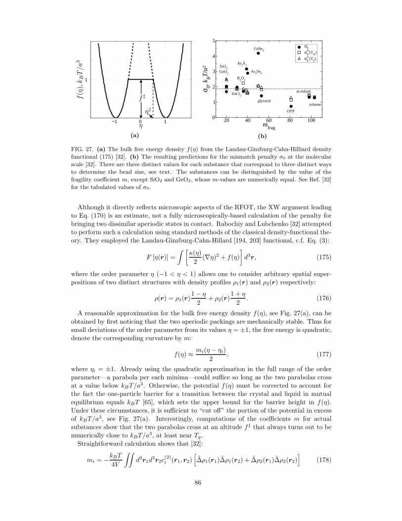
−1 0 1

1

η

f(η

),k

BT

/a3

η‡

f ‡

(a)

20 40 60 80 100m

frag

0

1

2

3

4

5

σ 0, kBT

/a²

σ0

σ0sc

(TK)

σ0sc

(T0)

SiO2

GeO2

ZnCl2

B2O

3

As2S

3

As2Se

3

GeSe2

glycerol

OTP

m-toluid.

toluene

(b)

FIG. 27. (a) The bulk free energy density f(η) from the Landau-Ginzburg-Cahn-Hilliard density

functional (175) [32]. (b) The resulting predictions for the mismatch penalty σ0 at the molecular

scale [32]. There are three distinct values for each substance that correspond to three distinct ways

to determine the bead size, see text. The substances can be distinguished by the value of the

fragility coefficient m, except SiO2 and GeO2, whose m-values are numerically equal. See Ref. [32]

for the tabulated values of σ0.

Although it directly reflects microscopic aspects of the RFOT, the XW argument leading

to Eq. (170) is an estimate, not a fully microscopically-based calculation of the penalty for

bringing two dissimilar aperiodic states in contact. Rabochiy and Lubchenko [32] attempted

to perform such a calculation using standard methods of the classical density-functional the-

ory. They employed the Landau-Ginzburg-Cahn-Hillard [194, 203] functional, c.f. Eq. (3):

F [η(r)] =

∫ [κ(η)

2(∇η)2 + f(η)

]d3r, (175)

where the order parameter η (−1 < η < 1) allows one to consider arbitrary spatial super-

positions of two distinct structures with density profiles ρ1(r) and ρ2(r) respectively:

ρ(r) = ρ1(r)1− η

2+ ρ2(r)

1 + η

2. (176)

A reasonable approximation for the bulk free energy density f(η), see Fig. 27(a), can be

obtained by first noticing that the two aperiodic packings are mechanically stable. Thus for

small deviations of the order parameter from its values η = ±1, the free energy is quadratic,

denote the corresponding curvature by m:

f(η) ≈ mi(η − ηi)

2, (177)

where ηi = ±1. Already using the quadratic approximation in the full range of the order

parameter—a parabola per each minima—could suffice so long as the two parabolas cross

at a value below kBT/a3. Otherwise, the potential f(η) must be corrected to account for

the fact the one-particle barrier for a transition between the crystal and liquid in mutual

equilibrium equals kBT [65], which sets the upper bound for the barrier height in f(η).

Under these circumstances, it is sufficient to “cut off” the portion of the potential in excess

of kBT/a3, see Fig. 27(a). Interestingly, computations of the coefficients m for actual

substances show that the two parabolas cross at an altitude f ‡ that always turns out to be

numerically close to kBT/a3, at least near Tg.

Straightforward calculation shows that [32]:

mi = −kBT4V

∫∫d3r1d

3r2c(2)i (r1, r2)

[∆ρ1(r1)∆ρ1(r2) + ∆ρ2(r1)∆ρ2(r2)

](178)

86

and

κi =kBT

8V

∫∫d3r1d

3r2z212c

(2)i (r1, r2)

[∆ρ1(r1)∆ρ1(r2) + ∆ρ2(r1)∆ρ2(r2)

], (179)

where ∆ρ(r) ≡ ρ1(r) − ρ2(r), c.f. Eq. (26). As expected, the coefficients at the quadratic

terms in the density functional couple density fluctuations that correspond to two-body

interactions; only fluctuations within individual states are coupled. The inter-state fluctu-

ations drop out because the structures are uncorrelated by construction. Since both states

1 and 2 are typical, we have m1 = m2 = m and κ1 = κ2 = κ.

Next, one may repeat the analysis analogously to that following Eq. (21), but also in-

cluding the shear component of the elastic free energy, in computing the pairwise cor-

relation function ρ(2)(r1, r2). Note that individual aperiodic structures are mechanically

(meta)stable and so µ > 0. This analysis results in the sum rule for the solid listed in

Eq. (65). Combined with the long-wavelength, Debye approximation for the vibrational

spectrum of our aperiodic solid and the generalised Ornstein-Zernike relation (62), this al-

lows one to write down the following expression for the Fourier image of the direct correlation

function from Eq. (18):

c(2)(k1,k2) ≃ −(2π)3δ(k1 + k2)θ(π/a− k)Mc2l

kBT ρNb, (180)

Note in this long-wavelength approximation, the direct correlation function turns out to

be translationally-invariant: c(2)(r1, r2) = c(2)(r1 − r2), which is generally not the case for

solids [82]. Note that in writing down the equation above, we have ignored the difference

between the isothermal and adiabatic speeds of longitudinal sound; this difference is not

substantial in solids, see our earlier comments following Eq. (65).

The density-density correlations within each phase are straightforwardly related to the

structure factor, by Eq. (61). Combining this with Eqs. (113), (180), (178), and (179) yields

the following simple expressions for the coefficients κ and m [32]:

κ =Mc2l a

−2S′(π/a)

24Nb, (181)

and

m =Mc2l4π2Nb

∫ πa

0

S(k)k2dk. (182)

where S′(k) = dS/dk.

Finally, we note that the surface tension coefficient σ0 corresponds to the mismatch

penalty at the molecular lengthscale, implying no surface tension renormalisation takes

place, as if the interface were entirely flat. Combining the standard formula for the surface

tension coefficient for a flat interface [195], σ =∫ 1

−1dη [2κf(η)]

1/2, and the two equations

above one can write down an explicit expression for the surface coefficient σ0 in terms of

measured quantities:

σ0 =kBT

a2

[Mc2l a

−1S′(π/a)

12NbkBT

]1/2

2−[

Mc2l8π2kBTNb

∫ πa

0

S(k)k2dk

]−1/2

, if m ≥ 2f ‡

(183)

σ0 =Mc2l a

−1

4√6Nb

[S′(π/a)

∫ πa

0

S(k)k2dk

]1/2, if m < 2f ‡ (184)

Note that the value of the factor in the curly brackets varies between 1 and 2.

87

Despite its relatively computational complexity and requiring the knowledge of many

experimental inputs, the RL formalism leading to Eqs. (181) and (182) has a side dividend

of allowing one to compute the correlation length in the landscape regime. By Eqs. (175)

and (177), the correlation length is simply√κ/m. According to RL’s estimates for actual

glass-formers, this length is of molecular dimensions, consistent with our earlier conclusions

that glassy liquids are far away from any sort of criticality.

The values of σ0 predicted by Eqs. (183) and (184) computed using experimentally deter-

mined values of the input parameters are plotted in Fig. 27(b), where they are compared

with the XW-predicted value 1.85kBT/a2 from Eq. (168). The filled circles correspond

to the calculation that employs the calorimetric bead count from Eq. (96). As noted in

Ref. [32], in instances where the σ0 value differed particularly significantly from the XW

prediction, the value of the configurational entropy at Tg also turned out to differ quite a

bit from the XW prediction that sc(Tg) ≈ 32/ ln(τ(Tg)/τ0), see Eq. (170). (Such differences

seem to come up often for substances with a significant degree of local ordering, such as the

chalcogenide alloys [54].) This suggests that the bead count may be off for these specific

substances. To test for the significance of the precise bead count, Rabochiy and Lubchenko

also determined the bead count self-consistently by requiring that the barrier from Eq. (164)

yield exactly kBT ln(3600/10−12), which corresponds to the glass transition on 1 hr scale.

The resulting bead count depends on whether the temperature T0 or TK is used for the

location of the putative Kauzmann state. The values of σ0 corresponding to both ways to

determine the bead count self-consistently are shown in Fig. 27(b) with squares (TK) and

triangles (T0). The self-consistently determined bead count turned out to be chemically

reasonable in all cases, except for OTP.

The general agreement between the σ0 values for different substances and the XW-

estimate, even for the calorimetrically determined bead size, is notable. On the one hand,

there would appear to be little a priori reason for a complicated combination of several

material constants to be so consistent among chemically-distinct substances. On the other

hand, one expects that the several approximations involved and some uncertainty in the

experimental input parameters, especially the structure factor, would introduce a potential

source of error in the final result, see detailed discussion in Ref. [32]. In any event, it is

an important corollary of the XW calculation that despite apparent differences in detailed

interactions among distinct substances, the value of σ0 is expected to be relatively universal

in that it can be expressed approximately through very few materials constants.

Elastic constants enter the expressions (183) and (184), similarly to Eq. (155) but in

a more complicated way. Still, in Eq.(183), which applies when m ≥ 2f ‡, i.e., when the

“ledge” in the f(η) is present (Fig. 27(a)), the resulting barrier clearly has a contribution

that is linear in the bulk modulus.

We have thus discussed three distinct approximations for the mismatch penalty in this

Subsection. The Xia-Wolynes [31] (XW) approximation (168) and Rabochiy-Lubchenko [32]

(RL) approximation (183)-(184) for σ0 can be combined with Eq. (164) to compute the free

energy barrier for activated transport in glassy liquids in an extended temperature range.

This was accomplished recently by Rabochiy, Wolynes, and Lubchenko [33] (RWL) for

eight specific substances. Likewise, the barrier can be computed, in principle, using the

Lubchenko-Rabochiy [34] (LR) approximation for the coefficient γ, Eq. (155), combined

with Eq. (154). The simplified form (159) only requires the knowledge of two experimental

quantities, which has enabled LR to estimate the barrier for seven actual substances. In

Fig. 28(a) we display the values for the barrier, as a function of temperature, as predicted by

all three approximations for a specific substance (m-toluidine). We plot the barriers within

the dynamical range representative of actual liquids, viz. ln(τ/τ0) ≤ 35.7, which corresponds

to a glass transition on 1 hr time scale and τ0 = 1 ps. This way, the error of the approxima-

tion exhibits itself through an error in the temperature corresponding to a particular value

88

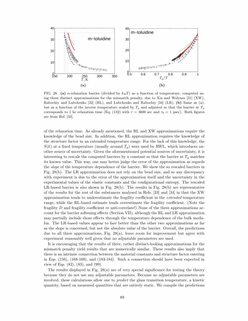
150 200 250 300 3500

10

20

30

40

T, K

m−toluidine

(a)

0.5 0.6 0.7 0.8 0.9 10

10

20

30

40

Tg/T

m−toluidine

(b)

FIG. 28. (a) α-relaxation barrier (divided by kBT ) as a function of temperature, computed us-

ing three distinct approximations for the mismatch penalty, due to Xia and Wolynes [31] (XW),

Rabochiy and Lubchenko [32] (RL), and Lubchenko and Rabochiy [34] (LR). (b) Same as (a),

but as a function of the inverse temperature scaled by Tg and adjusted so that the barrier at Tg

corresponds to 1 hr relaxation time (Eq. (132) with τ = 3600 sec and τ0 = 1 psec). Both figures

are from Ref. [33].

of the relaxation time. As already mentioned, the RL and XW approximations require the

knowledge of the bead size. In addition, the RL approximation requires the knowledge of

the structure factor in an extended temperature range. For the lack of this knowledge, the

S(k) at a fixed temperature (usually around Tg) were used by RWL, which introduces an-

other source of uncertainty. Given the aforementioned potential sources of uncertainty, it is

interesting to rescale the computed barriers by a constant so that the barrier at Tg matches

its known value. This way, one may better judge the error of the approximation as regards

the slope of the temperature dependence of the barrier. We show the so rescaled barriers in

Fig. 28(b). The LR approximation does not rely on the bead size, and so any discrepancy

with experiment is due to the error of the approximation itself and the uncertainty in the

experimental values of the elastic constants and the configurational entropy. The rescaled

LR-based barrier is also shown in Fig. 28(b). The results in Fig. 28(b) are representative

of the results for the rest of the substances analysed in Refs. [33] and [34] in that the XW

approximation tends to underestimate the fragility coefficient in the extended temperature

range, while the RL-based estimate tends overestimate the fragility coefficient. (Note the

fragility D and fragility coefficient m anti-correlate!) None of the three approximations ac-

count for the barrier softening effects (Section VII), although the RL and LR approximation

may partially include those effects through the temperature dependence of the bulk modu-

lus. The LR-based values appear to fare better than the other two approximations as far

as the slope is concerned, but not the absolute value of the barrier. Overall, the predictions

due to all three approximations, Fig. 28(a), leave room for improvement but agree with

experiment reasonably well given that no adjustable parameters are used.

It is encouraging that the results of three, rather distinct-looking approximations for the

mismatch penalty yield results that are numerically similar. These results also imply that

there is an intrinsic connection between the material constants and structure factor entering

in Eqs. (156), (168-169), and (183-184). Such a connection should have been expected in

view of Eqs. (82), (83), and (99).

The results displayed in Fig. 28(a) are of very special significance for testing the theory

because they do not use any adjustable parameters. Because no adjustable parameters are

involved, these calculations allow one to predict the glass transition temperature, a kinetic

quantity, based on measured quantities that are entirely static. We compile the predictions

89

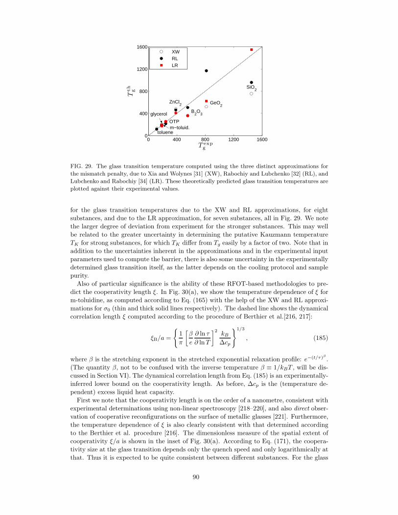
0 400 800 1200 16000

400

800

1200

1600

T expg

Tth

g

XWRLLR

glycerol

m−toluid.toluene

OTP

ZnCl2

B2O

3

GeO2

SiO2

FIG. 29. The glass transition temperature computed using the three distinct approximations for

the mismatch penalty, due to Xia and Wolynes [31] (XW), Rabochiy and Lubchenko [32] (RL), and

Lubchenko and Rabochiy [34] (LR). These theoretically predicted glass transition temperatures are

plotted against their experimental values.

for the glass transition temperatures due to the XW and RL approximations, for eight

substances, and due to the LR approximation, for seven substances, all in Fig. 29. We note

the larger degree of deviation from experiment for the stronger substances. This may well

be related to the greater uncertainty in determining the putative Kauzmann temperature

TK for strong substances, for which TK differ from Tg easily by a factor of two. Note that in

addition to the uncertainties inherent in the approximations and in the experimental input

parameters used to compute the barrier, there is also some uncertainty in the experimentally

determined glass transition itself, as the latter depends on the cooling protocol and sample

purity.

Also of particular significance is the ability of these RFOT-based methodologies to pre-

dict the cooperativity length ξ. In Fig. 30(a), we show the temperature dependence of ξ for

m-toluidine, as computed according to Eq. (165) with the help of the XW and RL approxi-

mations for σ0 (thin and thick solid lines respectively). The dashed line shows the dynamical

correlation length ξ computed according to the procedure of Berthier et al.[216, 217]:

ξB/a =

1

π

[β

e

∂ ln τ

∂ lnT

]2kB∆cp

1/3

, (185)

where β is the stretching exponent in the stretched exponential relaxation profile: e−(t/τ)β .

(The quantity β, not to be confused with the inverse temperature β ≡ 1/kBT , will be dis-

cussed in Section VI). The dynamical correlation length from Eq. (185) is an experimentally-

inferred lower bound on the cooperativity length. As before, ∆cp is the (temperature de-

pendent) excess liquid heat capacity.

First we note that the cooperativity length is on the order of a nanometre, consistent with

experimental determinations using non-linear spectroscopy [218–220], and also direct obser-

vation of cooperative reconfigurations on the surface of metallic glasses [221]. Furthermore,

the temperature dependence of ξ is also clearly consistent with that determined according

to the Berthier et al. procedure [216]. The dimensionless measure of the spatial extent of

cooperativity ξ/a is shown in the inset of Fig. 30(a). According to Eq. (171), the coopera-

tivity size at the glass transition depends only the quench speed and only logarithmically at

that. Thus it is expected to be quite consistent between different substances. For the glass

90

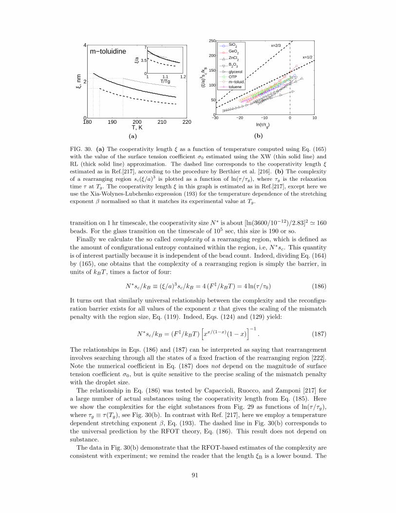
180 190 200 210 2200

2

4

T, K

ξ, n

m 1 1.1 1.20

3.5

7

T/Tg

ξ/a

m−toluidine

(a)

−30 −20 −10 0 100

50

100

150

200

250

ln(τ/τg)

(ξ/a

)3 s c/kB

SiO2

GeO2

ZnCl2

B2O

3

glycerolOTPm−toluid.toluene

x=2/3

x=1/2

(b)

FIG. 30. (a) The cooperativity length ξ as a function of temperature computed using Eq. (165)

with the value of the surface tension coefficient σ0 estimated using the XW (thin solid line) and

RL (thick solid line) approximation. The dashed line corresponds to the cooperativity length ξ

estimated as in Ref.[217], according to the procedure by Berthier et al. [216]. (b) The complexity

of a rearranging region sc(ξ/a)3 is plotted as a function of ln(τ/τg), where τg is the relaxation

time τ at Tg. The cooperativity length ξ in this graph is estimated as in Ref.[217], except here we

use the Xia-Wolynes-Lubchenko expression (193) for the temperature dependence of the stretching

exponent β normalised so that it matches its experimental value at Tg.

transition on 1 hr timescale, the cooperativity size N∗ is about [ln(3600/10−12)/2.83]2 ≃ 160

beads. For the glass transition on the timescale of 105 sec, this size is 190 or so.

Finally we calculate the so called complexity of a rearranging region, which is defined as

the amount of configurational entropy contained within the region, i.e, N∗sc. This quantityis of interest partially because it is independent of the bead count. Indeed, dividing Eq. (164)

by (165), one obtains that the complexity of a rearranging region is simply the barrier, in

units of kBT , times a factor of four:

N∗sc/kB ≡ (ξ/a)3sc/kB = 4 (F ‡/kBT ) = 4 ln(τ/τ0) (186)

It turns out that similarly universal relationship between the complexity and the reconfigu-

ration barrier exists for all values of the exponent x that gives the scaling of the mismatch

penalty with the region size, Eq. (119). Indeed, Eqs. (124) and (129) yield:

N∗sc/kB = (F ‡/kBT )[xx/(1−x)(1− x)

]−1

. (187)

The relationships in Eqs. (186) and (187) can be interpreted as saying that rearrangement

involves searching through all the states of a fixed fraction of the rearranging region [222].

Note the numerical coefficient in Eq. (187) does not depend on the magnitude of surface

tension coefficient σ0, but is quite sensitive to the precise scaling of the mismatch penalty

with the droplet size.

The relationship in Eq. (186) was tested by Capaccioli, Ruocco, and Zamponi [217] for

a large number of actual substances using the cooperativity length from Eq. (185). Here

we show the complexities for the eight substances from Fig. 29 as functions of ln(τ/τg),

where τg ≡ τ(Tg), see Fig. 30(b). In contrast with Ref. [217], here we employ a temperature

dependent stretching exponent β, Eq. (193). The dashed line in Fig. 30(b) corresponds to

the universal prediction by the RFOT theory, Eq. (186). This result does not depend on

substance.

The data in Fig. 30(b) demonstrate that the RFOT-based estimates of the complexity are

consistent with experiment; we remind the reader that the length ξB is a lower bound. The

91

100

101

102

103

104

105

106

107

108

τα

ov/τ

0

0

1

2

3

4

5

6

7

8

9

ξ 4ov

KA

WCA

IPL

HARD

HARM

ξ4

ov = 2.6

τα

s /τ

α

ov

(a)

0.5 0.6 0.7 0.8 0.9 11

1.2

1.4

1.6

1.8

2

2.2

2.4

2.6

T

ξ

3d KALJ

λmin

Scaling Length Scale

PTS Length Scale from Hocky et. al.

PTS Length Scale

(b)

FIG. 31. (a) The dependence of the four-point correlation length on the relaxation time, according

to computational studies by Flenner, Staley, and Szamel [223]. The fitted solid line has slope 1,

the dashed line slope 2/3. (b) Comparison between the point-to-set length and the extent λmin of

marginally stable harmonic modes in the inherent structures derived from samples equilibrated at

temperature T , from Biroli, Karmakar, and Procaccia [224]. The blue triangles give data due to

Hocky, Markland, and Reichman [225].

complexity graph also allows one to test the RFOT-predicted value of the scaling exponent

x for the mismatch penalty from Eq. (119). Indeed, if the exponent were equal to its

conventional value 2/3, the numerical coefficient[xx/(1−x)(1− x)

]−1in Eq. (187) would be

equal to 6.75, which significantly exceeds its value of 4 for x = 1/2, see Fig. 30(b). The

exponent 1/2 is clearly much more consistent with observation.

The complexity trends exhibited by actual liquids directly contradict the basic premise of

the Adam-Gibbs (AG) argument [156] on the connection between the configurational entropy

and relaxation rates in liquids. In short, Adam and Gibbs posited that the reconfiguration

barrier is determined by the enthalpic cost of deforming a region of a specific size. AG

argued the size should be such that the liquid has exactly two structural states available to

the region: N∗sc = ln 2. Such a view would be probably adequate at high temperatures,

however clearly fails for actual substances: First, given that sc is of order kB per particle,

the AG argument predicts the dynamical size that is too small. Second, the total entropy

content of a reconfiguring region, N∗sc, clearly depends on the temperature, in contrast

with the premise of Adam and Gibbs. Aside from these shortcomings, the AG ideas must

be credited for bringing attention to the possibility of an intrinsic connection between the

thermodynamics and kinetics in glassy liquids and for spurring much experimental work

that has studied this connection empirically. In any event, it should be clear to the reader

that the RFOT theory is not a variation on the phenomenological Adam-Gibbs scenario, as

is often mistakenly stated in the literature, but is a constructive argument.

On a somewhat related note, the data in Fig. 30 can be used to refute the premise of the

so called “shoving model,” which postulates that the reconfiguration barrier is determined

by the product of an elastic modulus and the volume of the rearranging region, which is

assumed to be fixed [212–214], in direct contradiction with Eq. (171), which predicts the

region’s volume changes by at least factor of a few hundred, within the dynamical range of

a typical experiment. (The quantity ln(τ/τ0) changes between 0 and 35 or so, in Eq. (171).

Alternatively, the configurational entropy per bead changes between 1.5 and 0.8 or so.)

Despite system-specific deviations of the predicted values for the barrier and the cooper-

ativity size from experiment, it is clear that the predictions of the RFOT theory are consis-

92

tent with observation both with regard to the absolute value of the parameters and the key

scaling relationships. Given this consistency with measurement on actual substances, the

reader may reasonably wonder if similar trends have been observed in computer simulations

of glassy liquids. It appears that at present, simulations are largely in the mode-coupling

regime and are only beginning to reach into the activated regime. Recent simulations on a

variety of model binary mixtures by Flenner et al. [223], indicate that the dependence of the

dynamic correlation length ξ4 on log τ can be well fit by a power law with the exponent 1

over the full temperature range. Still, the low-temperature flank of the data are more con-

sistent with the exponent 2/3, see Fig. 31. This is exactly what the RFOT theory predicts

for the scaling of the cooperativity length ξ in the activated transport regime, see Eq. (171).

Note that for the conventional scaling of the mismatch with the region size x = 2/3, the

exponent on the Flenner et al. plot would be equal 1/2, by Eqs. (129) and (126). The

four-point correlation length ξ4 from Fig. 31 is readily evaluated in simulations and, at the

same time, is naturally computed in field-theoretical approaches such as the mode-coupling

theory. The latter, however, has not been extended to the landscape regime characterised

by an exponential multiplicity of free energy minima. In meanfield, the correlation length

ξ4 of the MCT diverges at the temperature TA thus signalling the emergence of macroscopic

rigidity. As already mentioned and will be discussed in more detail in Section VII, the es-

tablishment of such macroscopic rigidity is avoided, owing to the activated reconfigurations,

because the metastable structures do not extend beyond the reconfiguration size ξ. Conse-

quently, while the length ξ represents a trivial lower bound on ξ4 above the crossover, it is

a non-trivial upper bound on ξ4 sufficiently below the crossover. A semi-phenomenological

way to estimate ξ4 within the RFOT theory, through spatial correlations in the mobility

field, has been discussed by Wisitsorasak and Wolynes [226] (see their Eqs. (14)-(16)); it

appears from the latter work that the lengths ξ4 and ξ are asymptotically equal as T tends

to TK . The mobility field that will be discussed in the context of glass rejuvenation, see

Section VIII B.

One way to quantify the spatial extent of the cooperativity—in a simulation—that is the

closest in spirit to the present formalism comes about in the library [40] or the Bouchaud-

Biroli construction [202], but goes back to the concept of the entropic droplet developed

by Wolynes and coworkers in the 1980s [30, 181]. Take a typical configuration and fix

particles outside a compact region, up to vibration. Now perform this procedure for regions

of various size. The size at which exactly two states are available corresponds with the

cooperativity length of the library construction and is often called the point-to-set length

ξPS . Alternatively, one may fix particles outside of a compact region not at positions

corresponding to an equilibrated liquid but, instead, at some generic positions. This length

can be shown to be equivalent to ξPS for a large enough region [227]. Equilibration of

the thus confined liquid is computationally difficult, and so only rather small system sizes

have been investigated. At any rate, the cooperativity length does increase with lowering

temperature, see Fig. 31(b). This confirms the basic notion that the lower the temperature,

the fewer states are available to a liquid region and the larger region must rearrange to find

an alternative structural state. Incidentally, the relative difficulty of equilibrating a region in

a confined geometry, as compared with periodic boundary conditions, is consistent with the

earlier comment that the present day simulations are only beginning to enter the landscape

regime. Indeed, subjecting a liquid to a rough wall is equivalent to imposing a quasi-static

field similar to that imposed by a long-lived structure.

We thus observe that a finite-size system with pinned surroundings can in fact run out of

configurational degrees of freedom—thus effectively undergoing a Kauzmann-like crisis—at

a finite value of the bulk configurational entropy. According to the library (or Bouchaud-

Biroli) construction, this finite value of the configurational entropy, s∗c , can be evaluated

with the help of Eq. (124) by setting N∗ at the system size N , thus yielding s∗c = γ/TN1−x.

93

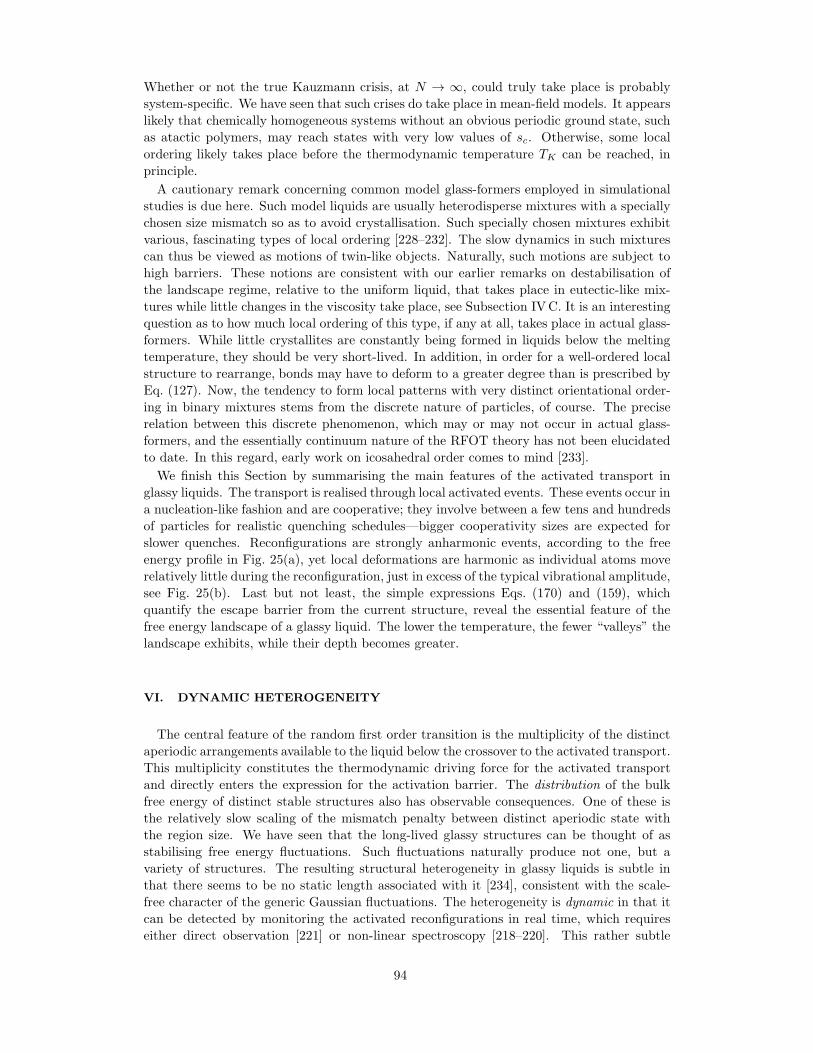
Whether or not the true Kauzmann crisis, at N → ∞, could truly take place is probably

system-specific. We have seen that such crises do take place in mean-field models. It appears

likely that chemically homogeneous systems without an obvious periodic ground state, such

as atactic polymers, may reach states with very low values of sc. Otherwise, some local

ordering likely takes place before the thermodynamic temperature TK can be reached, in

principle.

A cautionary remark concerning common model glass-formers employed in simulational

studies is due here. Such model liquids are usually heterodisperse mixtures with a specially

chosen size mismatch so as to avoid crystallisation. Such specially chosen mixtures exhibit

various, fascinating types of local ordering [228–232]. The slow dynamics in such mixtures

can thus be viewed as motions of twin-like objects. Naturally, such motions are subject to

high barriers. These notions are consistent with our earlier remarks on destabilisation of

the landscape regime, relative to the uniform liquid, that takes place in eutectic-like mix-

tures while little changes in the viscosity take place, see Subsection IVC. It is an interesting

question as to how much local ordering of this type, if any at all, takes place in actual glass-

formers. While little crystallites are constantly being formed in liquids below the melting

temperature, they should be very short-lived. In addition, in order for a well-ordered local

structure to rearrange, bonds may have to deform to a greater degree than is prescribed by

Eq. (127). Now, the tendency to form local patterns with very distinct orientational order-

ing in binary mixtures stems from the discrete nature of particles, of course. The precise

relation between this discrete phenomenon, which may or may not occur in actual glass-

formers, and the essentially continuum nature of the RFOT theory has not been elucidated

to date. In this regard, early work on icosahedral order comes to mind [233].

We finish this Section by summarising the main features of the activated transport in

glassy liquids. The transport is realised through local activated events. These events occur in

a nucleation-like fashion and are cooperative; they involve between a few tens and hundreds

of particles for realistic quenching schedules—bigger cooperativity sizes are expected for

slower quenches. Reconfigurations are strongly anharmonic events, according to the free

energy profile in Fig. 25(a), yet local deformations are harmonic as individual atoms move

relatively little during the reconfiguration, just in excess of the typical vibrational amplitude,

see Fig. 25(b). Last but not least, the simple expressions Eqs. (170) and (159), which

quantify the escape barrier from the current structure, reveal the essential feature of the

free energy landscape of a glassy liquid. The lower the temperature, the fewer “valleys” the

landscape exhibits, while their depth becomes greater.

VI. DYNAMIC HETEROGENEITY

The central feature of the random first order transition is the multiplicity of the distinct

aperiodic arrangements available to the liquid below the crossover to the activated transport.

This multiplicity constitutes the thermodynamic driving force for the activated transport

and directly enters the expression for the activation barrier. The distribution of the bulk

free energy of distinct stable structures also has observable consequences. One of these is

the relatively slow scaling of the mismatch penalty between distinct aperiodic state with

the region size. We have seen that the long-lived glassy structures can be thought of as

stabilising free energy fluctuations. Such fluctuations naturally produce not one, but a

variety of structures. The resulting structural heterogeneity in glassy liquids is subtle in

that there seems to be no static length associated with it [234], consistent with the scale-

free character of the generic Gaussian fluctuations. The heterogeneity is dynamic in that it

can be detected by monitoring the activated reconfigurations in real time, which requires

either direct observation [221] or non-linear spectroscopy [218–220]. This rather subtle

94

type of dynamic heterogeneity is distinct from but is often confused with a simpler kind

of dynamic heterogeneity, which is also intrinsic to glassy liquids and leads to observable

consequences in terms of spatially distributed relaxation rates. This we discuss next.

A. Correlation between non-exponentiality of liquid relaxation and fragility

According to Eqs. (129) and (164), the reconfiguration barrier is determined by the en-

tropy content of the local region. If fewer states are available, the escape time from the

current configurations is longer. This is straightforward to rationalise using the landscape

picture of the free energy surface of glassy liquids: Because the entropy is a monotonically

increasing function of enthalpy, entropy-poor states are also likely to be correspond to deeper

“valleys” in the landscape, thus implying a higher barrier must be surmounted in order to

escape from the valley. Thus, by Eqs. (129) and (164), the escape barrier—and hence relax-

ation rate—will fluctuate in reflection of local fluctuations in the configurational entropy.

Xia and Wolynes [38] exploited this idea to estimate a lower bound on the barrier fluctuation

in glassy liquids. (Local fluctuations in the mismatch penalty, if any, will also contribute

to the barrier fluctuation.) By this argument, the relative value of local fluctuation in the

escape barrier is given by:

δF ‡

F ‡mp

=δS∗

c

S∗c

=1

2√D, (188)

where S∗c ≡ scN

∗ is the configurational entropy of a single cooperative region and the index

“mp” signifies “most probable.” In the first equality, we assume that S∗c is Gaussianly dis-

tributed. The second equality gives the relative fluctuation of the configurational entropy for

a region of size ξ and is seen as follows: On the one hand, δS∗c =

√kB∆C∗

p =√kB∆cpN∗,

based on the general expression for entropy fluctuations: δS =√kBCp [55] and remember-

ing that ∆Cp corresponds to the excess liquid heat capacity relative to the crystal. On the

other hand, sc√N∗ = (γ/T ) by Eq. (124) with x = 1/2. Combined with Eqs. (94) and (98),

this yields the second equality in Eq. (188). It is interesting that the value x = 1/2 of the

scaling exponent for the mismatch penalty is unique in that it is the only value at which

the relative value of entropy fluctuations of a cooperative region is independent of its size:

δS∗c /S

∗c ∝ (T − TK)(2x−1). (For the latter estimate, one has to assume the “generalised”

form of the VFT law τ = τ0 exp[D/(T/TK − 1)x/(1−x)], see Eq. (129)).

Assuming the barrier distribution is Gaussian, it is straightforward to show [38] that the

exponential relaxation profile averaged over the barrier distribution yields approximately a

stretched-exponential:

⟨e−t/τ

⟩≈ e−(t/τmp)

β

, (189)

where the stretching exponent is determined by the width of the barrier distribution and

temperature: β = [1 + (δF ‡/kBT )2]−1/2 thus yielding

β =

1 +(F ‡mp/kBT

2√D

)2

−1/2

. (190)

In view of the near universality of the F ‡mp/kBT ratio near the glass transition, the above

equation implies the stretching exponent β is a simple function of the fragility D. The func-

tion is particularly simple for fragile substances, for which D is relatively small: β ∝√D.

The predictions due to Eq. (190) for the glass transition on 104 sec timescale, F ‡mp/kBT ≃

ln(104/10−12) ≈ 37, are shown in Fig. 32(a) with the dashed line. The agreement is only

95

2 4 6 8 10 12 14

0.2

0.4

0.6

0.8

1

D

β

1/ 2

*

Silicate Flint GlassPVC

Zn Cl 2

2

2

GeO

SiO

O - terphenyl

(a)

3.75 4.00 4.25 4.50 4.75 5.00 5.25

0

0.2

0.4

0.6

1000/T

β

(b)

FIG. 32. (a) The exponent β from the stretched-exponential relaxation profile e−(t/τ)β charac-

teristic of glassy liquids plotted against the square root of fragility D, as predicted by the RFOT

theory [38]. The dashed line corresponds to the simplest assumption of the Gaussianly distributed

barrier, while the solid line is obtained using the more complicated form in Eq. (191) that takes

into account the “facilitation” effect, by which a very slow region is unlikely to be exclusively sur-

rounded by comparably slow regions and thus will relax not slower than a typical region. (b) Solid

line: RFOT-predicted temperature dependence of β for a fragile glass-former [38]. Dashed line:

experimental measurements of Dixon and Nagel and their extrapolation to lower temperatures for

o-terphenyl [235].

qualitative; the lack of quantitative agreement can be explained by the neglect of the follow-

ing, “facilitation”-like effect. XW argued that a region can be considered unrelaxed insofar

as the particles in both the region and its immediate environment have not moved; this is

non-meanfield effect. A given region may be very slow, but the probability that the imme-

diate surrounding is also slow is small. For the same reason in a coin-flipping experiment,

the probability of the persistence of a particular pattern, such as many tails in row, is small.

XW thus argued that using a Gaussian distribution for the barriers in excess of the most

probable value of the distribution is too simplistic. The simplest way to fix this is to replace

the r.h.s. of the barrier distribution by a delta function with the area equal to 1/2 and

centred at F ‡mp:

p1(F ) =e−(1/F−1)2/2δF 2

√2π(δF )2F 2

+1

2δ(F − 1), (191)

where F ≡ F/Fmp < 1+, and we took advantage of the temperature-independence of the

relative width in Eq. (188).

The resulting prediction for the β vs. D relation is shown as the solid line in Fig. 32(a).

The agreement is now much improved. Lubchenko [43] has pointed out, in a different

context, that an exponential barrier distribution yields a comparable agreement with ex-

periment, while also agreeing with the frequency-dependent dielectric response ǫ′′(ω). The

width of this distribution is approximately δF ‡/4, i.e. the average between the l.h.s. of the

original Gaussian and the delta function:

p(F ) =

c1F 2e−(1/F−1)2/2δF 2

, F ≤ Fe

c2F 2eF /(δF/4), Fe < F ≤ 1,

(192)

This leads to a simple formula that works as well as the more complicated XW form con-

96

sisting of a half-gaussian and a delta function:

β =

1 +(F ‡mp/kBT

8√D

)2

−1/2

. (193)

Regardless of the size of the facilitation effects and how they are treated, the RFOT theory

unambiguously predicts that given the same value of the relaxation time (or viscosity),

the stretching exponent β should be smaller for more fragile substances. At the same

time, relaxations in the uniform liquid are exponential. This implies that the temperature

dependence of β will the more pronounced the more fragile the substance. We note that

the questions of the determination of both the stretching exponent β and its temperature

dependence are not without controversy. Xia and Wolynes predictions for the temperature

dependence of β for a very fragile substance are shown in Fig. 32(b) alongside experimental

data for OTP [235]. These results are also consistent with large-scale simulations of OTP

by Eastwood et al. [236]. Now, the temperature dependence of β in many substances seems

to deviate significantly [237] from the steady dependence seen in Fig. 32(b). This can be

rationalised by the presence of beta-relaxations which overlap frequency-wise with alpha-

relaxation, see Fig. 3. Indeed, in the absence of intervening processes, the quantity β can be

inferred by either fitting the relaxation profiles in direct time or can be extracted from the

slope of the high-frequency wing of the α-relaxation peak in the Fourier transform of ǫ′′(ω),whereby ǫ′′(ω) ∼ ω−β [43]. Likewise, there will be one-to-one correspondence between the

width of the peak and the value of β. Clearly, the relatively high-frequency β-relaxation, if

present, will affect the apparent shape of the α-peak. (Note the “beta” in beta-relaxation

has nothing to do with the stretching exponent β from Eq. (193).) In contrast, the estimates

of Xia and Wolynes [38] pertain exclusively to alpha relaxation and do not extend to other

processes. Another, early source of confusion on the temperature dependence of β has been

discussed by the present author [43]. When measured in even mildly conducting liquids, the

α-relaxation peak in ǫ′′(ω) is largely masked by a divergence at zero frequency. At the same

time, the inverse of the dielectric susceptibility, called the dielectric modulusM(ω), remains

perfectly finite. There have been attempts to extract the value of β from the width of the

α-peak in M ′′(ω). This procedure often yields a temperature dependence of the quantity

β opposite from that in Fig. 32(b). This opposite T -dependence is an artifact of the finite

conductivity and does not pertain to the actual α-relaxation.

B. Violation of the Stokes-Einstein relation and decoupling of various processes

The diffusivity D (not to be confused with the fragility D from Eq. (98)) reflects the

efficiency of particle transport, in response to density fluctuations:

j = −D∇n, (194)

where j is the particle flux.

Diffusion of small molecules in a glassy liquid in the activated regime is qualitatively

different from largely collisional transport. Indeed, the motion of an individual bead, when

in the landscape regime, is completely slaved to the structural reconfigurations. A bead

typically moves a distance dL during a reconfiguration, Eq. (127), on average once per α-

relaxation time τloc. Here the index “loc” signifies that the waiting time is distributed and

generally differs from location to location, by Eq. (191) or its like. Suppose for a moment

the quantity τloc is not distributed. The relation between the particle displacement dL and

the waiting time τloc then implies the particle transport obeys the diffusion equation with

97

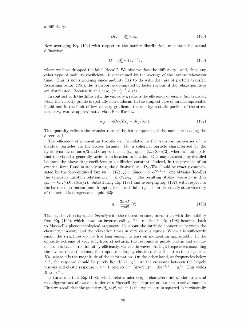
a diffusivity:

Dloc = d2L/6τloc. (195)

Now averaging Eq. (194) with respect to the barrier distribution, we obtain the actual

diffusivity:

D = (d2L/6)⟨τ−1

⟩, (196)

where we have dropped the label “local.” We observe that the diffusivity—and, thus, any

other type of mobility coefficient—is determined by the average of the inverse relaxation

time. This is not surprising since mobility has to do with the rate of particle transfer.

According to Eq. (196), the transport is dominated by faster regions, if the relaxation rates

are distributed. Because in this case,⟨τ−1

⟩−1< 〈τ〉.

In contrast with the diffusivity, the viscosity η reflects the efficiency ofmomentum transfer,

when the velocity profile is spatially non-uniform. In the simplest case of an incompressible

liquid and in the limit of low velocity gradients, the non-hydrostatic portion of the stress

tensor σij can be approximated via a Fick-like law:

σij = η(∂vi/∂xj + ∂vj/∂xi). (197)

This quantity reflects the transfer rate of the ith component of the momentum along the

direction j.

The efficiency of momentum transfer can be related to the transport properties of in-

dividual particles via the Stokes formula. For a spherical particle characterised by the

hydrodynamic radius a/2 and drag coefficient ζloc, ηloc = ζloc/(6πa/2), where we anticipate

that the viscosity generally varies from location to location. One may associate, by detailed

balance, the above drag coefficient to a diffusion constant. Indeed, in the presence of an

external force f and in steady state, the diffusive flux −Dloc∇n should be exactly compen-

sated by the force-induced flux vn = (f/ζloc)n. Since n ∝ efr/kBT , one obtains (locally)

the venerable Einstein relation ζloc = kBT/Dloc. The resulting Stokes’ viscosity is thus

ηloc = kBT/Dloc(6πa/2). Substituting Eq. (196) and averaging Eq. (197) with respect to

the barrier distribution (and dropping the “local” label) yields for the steady-state viscosity

of the actual heterogeneous liquid [43]:

η =2kBT

πad2L〈τ〉 . (198)

That is, the viscosity scales linearly with the relaxation time, in contrast with the mobility

from Eq. (196), which shows an inverse scaling. The relation in Eq. (198) hearkens back

to Maxwell’s phenomenological argument [85] about the intrinsic connection between the

elasticity, viscosity, and the relaxation times in very viscous liquids: When τ is sufficiently

small, the structures do not live long enough to pass on momentum appreciably. In the

opposite extreme of very long-lived structures, the response is purely elastic and so mo-

mentum is transferred infinitely efficiently, via elastic waves. At high frequencies exceeding

the inverse relaxation time, the response is largely elastic so that the stress tensor goes as

Ku, where u is the magnitude of the deformation. On the other hand, at frequencies below

τ−1, the response should be purely liquid-like: ηu. At the crossover between the largely

viscous and elastic response, ωτ ≃ 1, and so u ≃ (d/dt)[u(t = 0)e−t/τ ] = u/τ . This yields

K ≃ ητ−1.

It turns out that Eq. (198), which relates microscopic characteristics of the structural

reconfigurations, allows one to derive a Maxwell-type expression in a constructive manner.

First we recall that the quantity (dL/a)2, which is the typical strain squared, is intrinsically

98

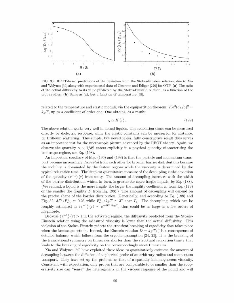
1 2 3 4 5 6 7

0.5

1

1.5

2

2.5

3

R / a

DD

tS

-E/

log

()

(a)

1 1.1 1.2 1.3 1.4

0

0.5

1

1.5

2

2.5

3

T/ Tg

DD

tS

-E

/lo

g(

)

(b)

FIG. 33. RFOT-based predictions of the deviation from the Stokes-Einstein relation, due to Xia

and Wolynes [39] along with experimental data of Cicerone and Ediger [220] for OTP. (a) The ratio

of the actual diffusivity to its value predicted by the Stokes-Einstein relation, as a function of the

probe radius. (b) Same as (a), but a function of temperature [39].

related to the temperature and elastic moduli, via the equipartition theorem: Ka3(dL/a)2 =

kBT , up to a coefficient of order one. One obtains, as a result:

η ≃ K 〈τ〉 . (199)

The above relation works very well in actual liquids. The relaxation times can be measured

directly by dielectric response, while the elastic constants can be measured, for instance,

by Brillouin scattering. This simple, but nevertheless, fully constructive result thus serves

as an important test for the microscopic picture advanced by the RFOT theory. Again, we

observe the quantity α ∼ 1/d2L enters explicitly in a physical quantity characterising the

landscape regime, see Eq. (198).

An important corollary of Eqs. (196) and (198) is that the particle and momentum trans-

port become increasingly decoupled from each other for broader barrier distributions because

the mobility is dominated by the fastest regions while the viscosity is determined by the

typical relaxation time. The simplest quantitative measure of the decoupling is the deviation

of the quantity⟨τ−1

⟩〈τ〉 from unity. The amount of decoupling increases with the width

of the barrier distribution, which, in turn, is greater for more fragile liquids, by Eq. (188).

(We remind, a liquid is the more fragile, the larger the fragility coefficient m from Eq. (173)

or the smaller the fragility D from Eq. (98).) The amount of decoupling will depend on

the precise shape of the barrier distribution. Generically, and according to Eq. (188) and

Fig. 32, δF ‡/F ‡mp ≃ 0.25 while F ‡

mp/kBT ≃ 37 near Tg. The decoupling, which can be

roughly estimated as⟨τ−1

⟩〈τ〉 ∼ e+δF ‡/kBT , thus could be as large as a few orders of

magnitude.

Because⟨τ−1

⟩〈τ〉 > 1 in the activated regime, the diffusivity predicted from the Stokes-

Einstein relation using the measured viscosity is lower than the actual diffusivity. This

violation of the Stokes-Einstein reflects the transient breaking of ergodicity that takes place

when the landscape sets in. Indeed, the Einstein relation D = kBT/ζ is a consequence of

detailed balance, which follows from the ergodic assumption [24, 25]. It is the breaking of

the translational symmetry on timescales shorter than the structural relaxation time τ that

leads to the breaking of ergodicity on the correspondingly short timescales.

Xia and Wolynes [39] have exploited these ideas to quantitatively estimate the amount of

decoupling between the diffusion of a spherical probe of an arbitrary radius and momentum

transport. They have set up the problem as that of a spatially inhomogeneous viscosity.

Consistent with expectation, only probes that are comparable to or smaller than the coop-

erativity size can “sense” the heterogeneity in the viscous response of the liquid and will

99

0.7 0.8 0.9 1T

g/T

10-9

10-6

10-3

100

103

secτ

mp

<τ>τ, ε"(ω)

<τ−1>−1

(a) (b)

FIG. 34. (a) Different relaxation times derived from the barrier distribution in Eq.(192), as func-

tions of temperature. δF = 0.25, corresponding to fragility D = 4 [43]. (b) Relaxation time

pertaining to the ionic conductivity, τσ, and the structural relaxation time τs. From Howell et

al. [238].

violate the Stokes-Einstein relation. Quantitative predictions of the extent of the violation,

due to Xia and Wolynes (XW), are shown in Fig. 33(a), alongside the experimental data of

Cicerone and Ediger [220], all near the glass transition. The agreement is good, especially

considering that no adjustable parameters were used. As already mentioned, the decoupling

goes roughly as e−δF ‡/kBT and should be greater for lower temperatures since the barrier

F ‡—and hence a measure of the barrier distribution width δF ‡ ∝ F ‡—increase with low-

ering temperature. This notion is borne out both in the RFOT-based predictions and in

observation, see Fig. 33(b). (To avoid confusion we note that XW used the “slip” boundary

conditions in their calculation, which engenders a distinct value of the numerical coefficient

in the Stokes formula from the preceding qualitative argument, viz., η = ζ/4πR.)

Lubchenko [43] has addressed the decoupling between ionic conductivity and momentum

transfer in ionic liquids such as CKN (40% Ca(NO3)2-60%KNO3). In such liquids, every

bead is charged. In the presence of an electric field, there is a non-zero net current density:

j = 〈j′〉 = 1

ξ3

⟨µT

τ

⟩, (200)

because the transition barrier, and hence the relaxation time are coupled to the electric field

E: τ−1(E) = τ−1(E = 0)(1 +µ‡TE/kBT ), while the the transition dipole moment µ‡

T of a

reconfiguring region is correlated with the overall transition dipole moment µT . A detailed

calculation yields for the ionic conductivity tensor:

σij = δij∆µ2

mol

8 a3kBT

⟨1

τ

⟩, (201)

where ∆µmol is the transition dipole moment of a single bead: |∆µmol| ∼ qdL, and q is the

bead charge. Not surprisingly, the above expression for the mobility of charged particles

has the same structure as that for the diffusivity in Eq. (196). The resulting temperature

dependence of the decoupling for a generic fragile substance is shown in Fig. 34(a), to be

compared with the decoupling between ionic transport and viscosity observed in KCN [238]

100

shown in Fig. 34(b). Fig. 34(a) also demonstrates that the relaxation time, as determined by

locating the peak in the imaginary part of the dielectric susceptibility ǫ′′(ω) is numerically

close to the typical relaxation time, and so is the most probable relaxation time.

Various other types of decoupling have been observed in viscous liquids and, in fact, have

been used to detect the crossover to the activated transport. We turn to this next.

VII. AT THE CROSSOVER FROM COLLISIONAL TO ACTIVATED TRANS-

PORT

Now that we have established a microscopic perspective on both the thermodynamics and

kinetics in the activated regime, we are ready to discuss how the landscape regime sets in, in

the first place. The crossover spans a dynamical range of a couple of decades in chemically-

bonded glassformers, which is much less than the full dynamical range of sixteen decades or

so accessible during a quench. Yet the crossover is a very important aspect of any microscopic

theory of the structural glass transition. It is the transition that ultimately underlies the

formation of the metastable structures and the eventual, complete loss of ergodicity that

takes place at the temperature Tg < Tcr. Unfortunately, the crossover is much harder

to describe quantitatively than the regime of well-developed activated transport because

the activated reconfigurations are no longer decoupled from the vibrations. One may say

that the activated reconfigurations are strongly affected by mode-coupling at the crossover.

Conversely, one may say the MCT-predicted slowing down becomes short-circuited by the

activated transition. Neither approach works quantitatively at the crossover, on its own, nor

is it clear at present how to marry the two in a formally satisfactory way. (See however the

earlier mentioned work in Refs. [166, 167] for phenomenological, hybrid approaches.) Despite

these complications, both quantitative and qualitative characteristics of the crossover can

be established by building on the microscopic picture of the activated transport reviewed

above.

Already the recognition that particle transport occurs by activation below the crossover

yields a testable prediction that the temperature dependence of the relaxation time for fragile

substances should not obey an Adam-Gibbs (AG) like expression in the full temperature

range between the melting temperature Tm and glass transition temperature Tg. This is

because the crossover temperature for sufficiently fragile liquids is below Tm. The elegant

analysis of Stickel et al. [239] demonstrates that, indeed, temperature dependences of α-

relaxation are well fitted by two distinct AG forms, in the low-T and high-T portions of the

full temperature interval Tg < T < Tm.

To actually estimate Tcr, one must first recognise that there will be significant corrections

to the RFOT-derived expression for the reconfiguration barrier, Eq. (154), upon approaching

the crossover from below. We reiterate that the crossover, which is centred at temperature

Tcr, is the finite-dimensional analog of the mean-field transition at temperature TA, at which

the liquid free energy F (α) from Eq. (53) develops a metastable minimum. As usual, the

transition is lowered in finite dimensions, compared with meanfield: Tcr < TA. Lubchenko

and Wolynes [35] (LW) have elucidated the origin of this lowering. They pointed out that

as one approaches from below the temperature TA, at which the mean-field free energy

F (α) has a spinodal, fluctuations in the order parameter α become increasingly strong.

The spinodal is illustrated by the thick solid line in Fig. 13(a). Thus the assumption that

each metastable minimum is long-living becomes progressively less reliable as the spinodal

is approached (from below); consequently, the expression (154) increasingly overestimates

the barrier.

In assessing the magnitude of the resulting barrier softening effects LW noted that the

mismatch penalty between distinct aperiodic minima scales with a positive power of the

101

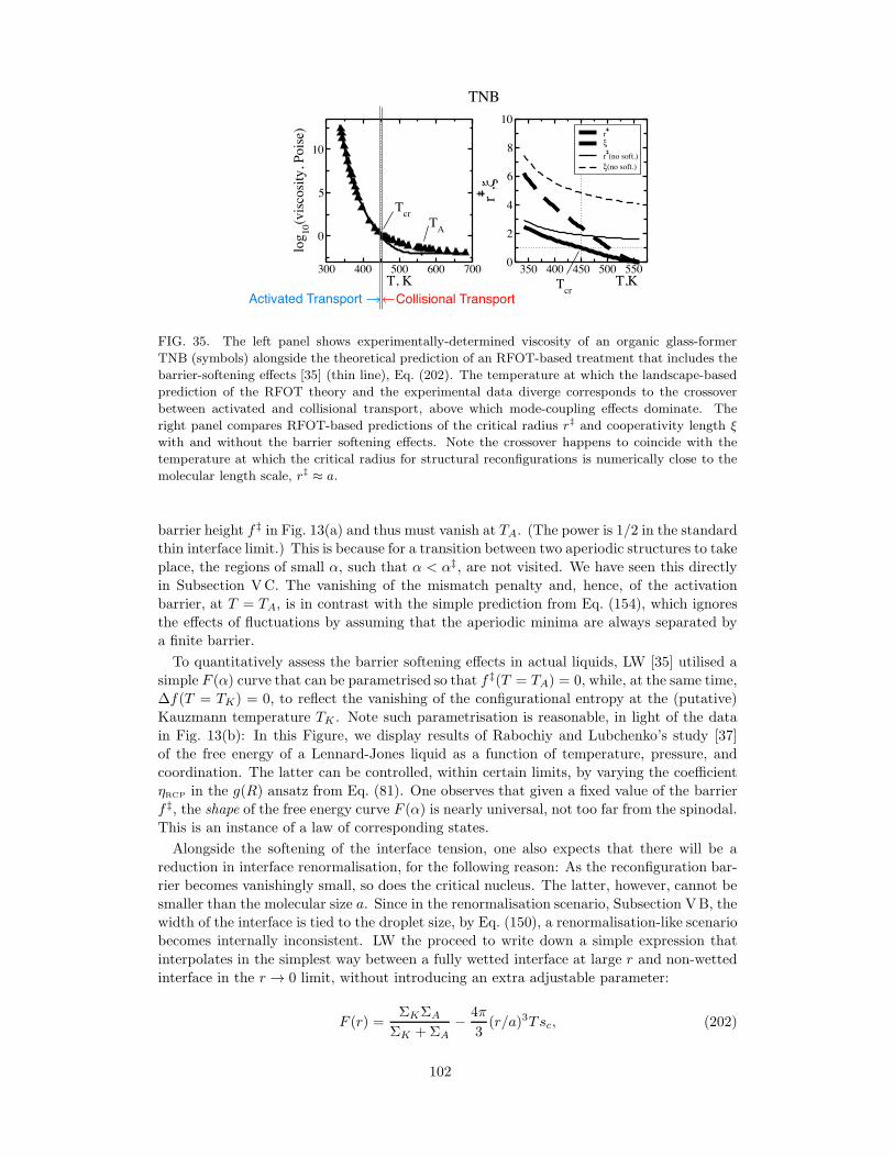
300 400 500 600 700T, K

0

5

10

log10(viscosity,Poise)

Tcr

Tcr

TA

TNB

350 400 450 500 550T,K

0

2

4

6

8

10

r,ξ

r

ξ

r(no soft.)

ξ(no soft.)

Collisional TransportActivated Transport

FIG. 35. The left panel shows experimentally-determined viscosity of an organic glass-former

TNB (symbols) alongside the theoretical prediction of an RFOT-based treatment that includes the

barrier-softening effects [35] (thin line), Eq. (202). The temperature at which the landscape-based

prediction of the RFOT theory and the experimental data diverge corresponds to the crossover

between activated and collisional transport, above which mode-coupling effects dominate. The

right panel compares RFOT-based predictions of the critical radius r‡ and cooperativity length ξ

with and without the barrier softening effects. Note the crossover happens to coincide with the

temperature at which the critical radius for structural reconfigurations is numerically close to the

molecular length scale, r‡ ≈ a.

barrier height f ‡ in Fig. 13(a) and thus must vanish at TA. (The power is 1/2 in the standard

thin interface limit.) This is because for a transition between two aperiodic structures to take

place, the regions of small α, such that α < α‡, are not visited. We have seen this directly

in Subsection VC. The vanishing of the mismatch penalty and, hence, of the activation

barrier, at T = TA, is in contrast with the simple prediction from Eq. (154), which ignores

the effects of fluctuations by assuming that the aperiodic minima are always separated by

a finite barrier.

To quantitatively assess the barrier softening effects in actual liquids, LW [35] utilised a

simple F (α) curve that can be parametrised so that f ‡(T = TA) = 0, while, at the same time,

∆f(T = TK) = 0, to reflect the vanishing of the configurational entropy at the (putative)

Kauzmann temperature TK . Note such parametrisation is reasonable, in light of the data

in Fig. 13(b): In this Figure, we display results of Rabochiy and Lubchenko’s study [37]

of the free energy of a Lennard-Jones liquid as a function of temperature, pressure, and

coordination. The latter can be controlled, within certain limits, by varying the coefficient

ηRCP in the g(R) ansatz from Eq. (81). One observes that given a fixed value of the barrier

f ‡, the shape of the free energy curve F (α) is nearly universal, not too far from the spinodal.

This is an instance of a law of corresponding states.

Alongside the softening of the interface tension, one also expects that there will be a

reduction in interface renormalisation, for the following reason: As the reconfiguration bar-

rier becomes vanishingly small, so does the critical nucleus. The latter, however, cannot be

smaller than the molecular size a. Since in the renormalisation scenario, Subsection VB, the

width of the interface is tied to the droplet size, by Eq. (150), a renormalisation-like scenario

becomes internally inconsistent. LW the proceed to write down a simple expression that

interpolates in the simplest way between a fully wetted interface at large r and non-wetted

interface in the r → 0 limit, without introducing an extra adjustable parameter:

F (r) =ΣKΣA

ΣK +ΣA− 4π

3(r/a)3Tsc, (202)

102

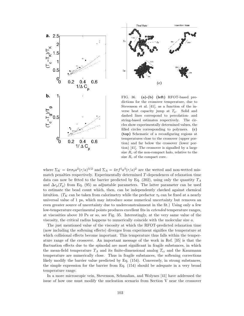
(c)

FIG. 36. (a)-(b) (left) RFOT-based pre-

dictions for the crossover temperature, due to

Stevenson et al. [41], as a function of the in-

verse heat capacity jump at Tg. Solid and

dashed lines correspond to percolation- and

string-based estimates respectively. The cir-

cles show experimentally determined values, the

filled circles corresponding to polymers. (c)

(top) Schematic of a reconfiguring regions at

temperatures close to the crossover (upper por-

tion) and far below the crossover (lower por-

tion) [41]. The crossover is signalled by a large

size Rs of the non-compact halo, relative to the

size Rc of the compact core.

where ΣK = 4πσ0a2(r/a)3/2 and ΣA = 4πf ‡a3(r/a)2 are the wetted and non-wetted mis-

match penalties respectively. Experimentally determined T -dependences of relaxation time

data can now be fitted to the barrier predicted by Eq. (202), using only the quantity TAand ∆cp(Tg) from Eq. (95) as adjustable parameters. The latter parameter can be used

to estimate the bead count which, then, can be independently checked against chemical

intuition. (TK can be taken from calorimetry while the prefactor τ0 can be fixed at a nearly

universal value of 1 ps, which may introduce some numerical uncertainty but removes an

even greater source of uncertainty due to underconstrainment in the fit.) Using only a few

low-temperature experimental points produces excellent fits in extended temperature ranges,

at viscosities above 10 Ps or so, see Fig. 35. Interestingly, at the very same value of the

viscosity, the critical radius happens to numerically coincide with the molecular size a.

The just mentioned value of the viscosity at which the RFOT-predicted relaxation time

(now including the softening effects) diverges from experiment signifies the temperature at

which collisional effects become important. This temperature thus falls within the temper-

ature range of the crossover. An important message of the work in Ref. [35] is that the

fluctuation effects due to the spinodal are most significant in fragile substances, in which

the mean-field temperature TA and its finite-dimensional analog Tcr and the Kauzmann

temperature are numerically close. Thus in fragile substances, the softening corrections

likely modify the barrier value predicted by Eq. (154). Conversely, in strong substances,

the simple expression for the barrier from Eq. (154) should be adequate in a very broad

temperature range.

In a more microscopic vein, Stevenson, Schmalian, and Wolynes [41] have addressed the

issue of how one must modify the nucleation scenario from Section V near the crossover

103

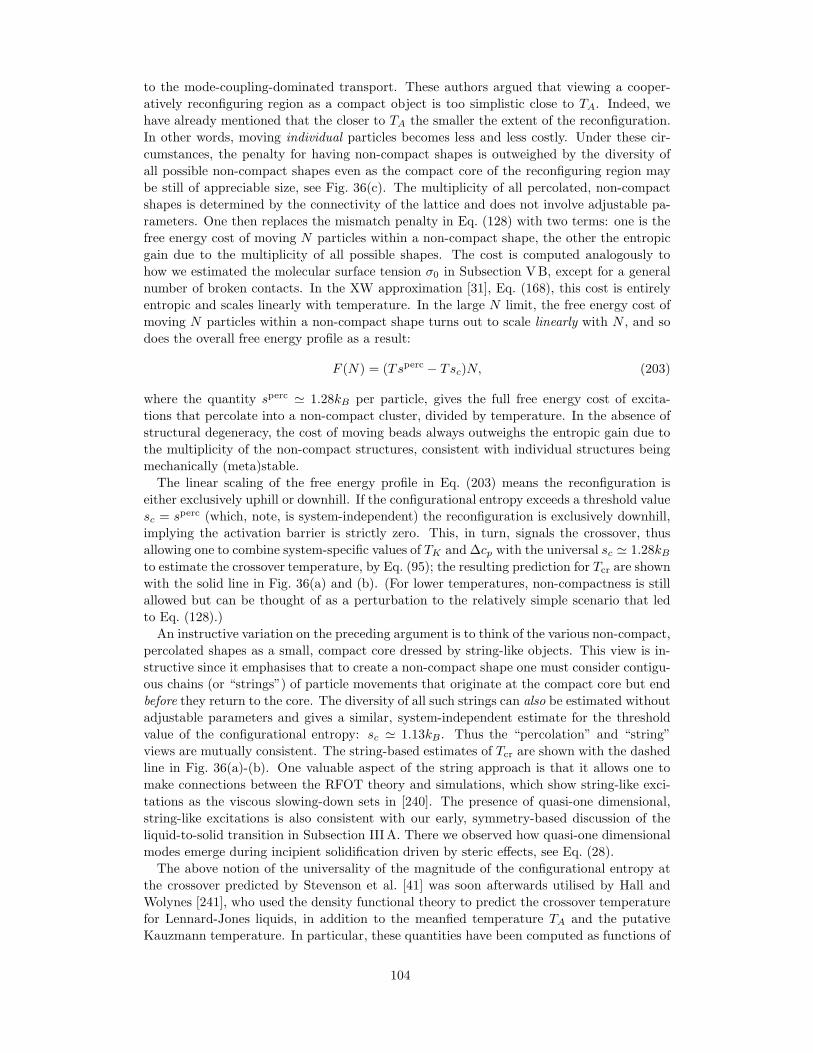
to the mode-coupling-dominated transport. These authors argued that viewing a cooper-

atively reconfiguring region as a compact object is too simplistic close to TA. Indeed, we

have already mentioned that the closer to TA the smaller the extent of the reconfiguration.

In other words, moving individual particles becomes less and less costly. Under these cir-

cumstances, the penalty for having non-compact shapes is outweighed by the diversity of

all possible non-compact shapes even as the compact core of the reconfiguring region may

be still of appreciable size, see Fig. 36(c). The multiplicity of all percolated, non-compact

shapes is determined by the connectivity of the lattice and does not involve adjustable pa-

rameters. One then replaces the mismatch penalty in Eq. (128) with two terms: one is the

free energy cost of moving N particles within a non-compact shape, the other the entropic

gain due to the multiplicity of all possible shapes. The cost is computed analogously to

how we estimated the molecular surface tension σ0 in Subsection VB, except for a general

number of broken contacts. In the XW approximation [31], Eq. (168), this cost is entirely

entropic and scales linearly with temperature. In the large N limit, the free energy cost of

moving N particles within a non-compact shape turns out to scale linearly with N , and so

does the overall free energy profile as a result:

F (N) = (Tsperc − Tsc)N, (203)

where the quantity sperc ≃ 1.28kB per particle, gives the full free energy cost of excita-

tions that percolate into a non-compact cluster, divided by temperature. In the absence of

structural degeneracy, the cost of moving beads always outweighs the entropic gain due to

the multiplicity of the non-compact structures, consistent with individual structures being

mechanically (meta)stable.

The linear scaling of the free energy profile in Eq. (203) means the reconfiguration is

either exclusively uphill or downhill. If the configurational entropy exceeds a threshold value

sc = sperc (which, note, is system-independent) the reconfiguration is exclusively downhill,

implying the activation barrier is strictly zero. This, in turn, signals the crossover, thus

allowing one to combine system-specific values of TK and ∆cp with the universal sc ≃ 1.28kBto estimate the crossover temperature, by Eq. (95); the resulting prediction for Tcr are shown

with the solid line in Fig. 36(a) and (b). (For lower temperatures, non-compactness is still

allowed but can be thought of as a perturbation to the relatively simple scenario that led

to Eq. (128).)

An instructive variation on the preceding argument is to think of the various non-compact,

percolated shapes as a small, compact core dressed by string-like objects. This view is in-

structive since it emphasises that to create a non-compact shape one must consider contigu-

ous chains (or “strings”) of particle movements that originate at the compact core but end

before they return to the core. The diversity of all such strings can also be estimated without

adjustable parameters and gives a similar, system-independent estimate for the threshold

value of the configurational entropy: sc ≃ 1.13kB. Thus the “percolation” and “string”

views are mutually consistent. The string-based estimates of Tcr are shown with the dashed

line in Fig. 36(a)-(b). One valuable aspect of the string approach is that it allows one to

make connections between the RFOT theory and simulations, which show string-like exci-

tations as the viscous slowing-down sets in [240]. The presence of quasi-one dimensional,

string-like excitations is also consistent with our early, symmetry-based discussion of the

liquid-to-solid transition in Subsection IIIA. There we observed how quasi-one dimensional

modes emerge during incipient solidification driven by steric effects, see Eq. (28).

The above notion of the universality of the magnitude of the configurational entropy at

the crossover predicted by Stevenson et al. [41] was soon afterwards utilised by Hall and

Wolynes [241], who used the density functional theory to predict the crossover temperature

for Lennard-Jones liquids, in addition to the meanfied temperature TA and the putative

Kauzmann temperature. In particular, these quantities have been computed as functions of

104

pressure and show good agreement with experiment.

We now return to the law of corresponding states illustrated in Fig. 13(b). Rabochiy and

Lubchenko [37] used this notion to argue that the crossover should take place at a universal

value of the farrier f ‡. Indeed, activated reconfigurations become essentially one-particle

events at the crossover, as we discussed earlier in this Section, implying fluctuations in the

order parameter α at different spots become mutually uncorrelated. Thus the local value

of the bulk density f(α)—corresponding to the free energy F (α)—fully characterises the

stability of a local region, regardless of its environment. In other words, the sample can be

thought of as a collection of uncorrelated, anharmonic degrees of freedom subject to a (free)

energy function f(α). Each such degree of freedom—and, hence, the aperiodic structures

themselves—become marginally stable when at the typical thermal displacement away from

the minimum, α is at its saddle point value α‡. In other words,⟨(α− α0)

2⟩1/2

= (α0 −α‡),times a factor of order 1. Combined with the near universality of the shape of f(α), this

implies that the crossover is signalled by a system-independent value of f ‡. This criterion can

be made more practical by noticing [37] that the (computed) f ‡ = const lines in the (p, T )

plane nearly coincide with the (computed) lines L = const, where L is the Lindemann ratio

from Eq. (80), where the lattice is now aperiodic. This is illustrated in Fig. 37(a). We thus

arrive, semi-phenomenologically, at a criterion that the crossover corresponds to a universal

value of the ratio of the vibrational displacement to particle spacing, irrespective of pressure

or temperature. This is in harmony with the systematic version of the Lindemann criterion

of melting [65], under which the vibrational displacement at the solid-liquid interface is a

universal quotient of the particle spacing, when the solid and liquid are in equilibrium. The

crossover also corresponds to an equilibrium between liquid and solid, except the latter solid

is now aperiodic. RL [37] took this notion further to determine the actual value of L that

signals the crossover. These authors have evaluated the values of the Lindemann ratio L

at the phase boundary for the liquid and the periodic crystal as a function of pressure (or

T ), the totality of which form a line in the (L, p, T ) space; this line is shown as the thick

solid line in Fig. 37(a). The L(p, T ) plane for the Lindemann ratio in the aperiodic crystal

mostly lies above the line L(p, T ) for the periodic crystal, but turns out to intersect it near

the triple point. Note the value of L at the triple point is unique for each substance. On

the other hand, the Lindemann ratio at the crossover is nearly unique, as just discussed.

Based on these two notions and the fact that the (L, p, T ) plane crosses the L(p, T ) line

near the triple point, RL surmised that the Lindemann ratio at the crossover Lcr should be

equal to its value at the triple point. The classical DFT, in the modified weighted density

approximation (MWDA), yields the value of 0.12 for Lcr [37]. The actual value of the

Lindemann ratio near the triple point of the Lennard-Jones system is

Lcr = 0.145, (204)

according to simulations [78]. This number will be of use in short order.

The above findings on the universality of the Lindemann displacement at the crossover

can be used to make several testable predictions. Several of these predictions rationalise the

pressure dependence of the fragility, depending on the degree of bonding directionality [37].

Here we limit ourselves to covering only two of these predictions.

As pressure is increased, any substance will behave more and more like that made of rigid

particles, in the absence of a structural transformation that would increase the coordination

in a discontinuous way. Under these circumstances, the external pressure becomes increas-

ingly close to the kinetic pressure, which corresponds to the amount of momentum a particle

transfers to its cage per unit time, per unit area: p ∼ 2(mvth)(vth/d0)/a2 ≃ 2(a/d0)nkBT ≃

2kBT/d0a2, thus implying p ≃ 2kBT

a21d0, where vth is the average thermal speed and d0 is

the confinement length of a particle in its cage. Since the confinement length is equal to

dL and, furthermore, is constant at the crossover, we obtain a simple estimate for pressure

105

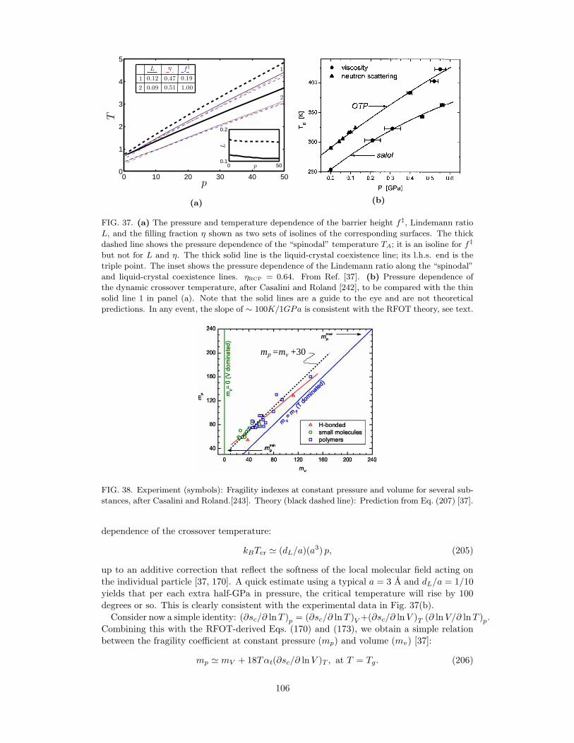
0 10 20 30 40 500

1

2

3

4

5

p

T

0 500.1

0.2

p

L

L η f‡ 1

2

1

2

0.12 0.47 0.19

0.09 0.51 1.00

(a) (b)

FIG. 37. (a) The pressure and temperature dependence of the barrier height f‡, Lindemann ratio

L, and the filling fraction η shown as two sets of isolines of the corresponding surfaces. The thick

dashed line shows the pressure dependence of the “spinodal” temperature TA; it is an isoline for f‡

but not for L and η. The thick solid line is the liquid-crystal coexistence line; its l.h.s. end is the

triple point. The inset shows the pressure dependence of the Lindemann ratio along the “spinodal”

and liquid-crystal coexistence lines. ηRCP = 0.64. From Ref. [37]. (b) Pressure dependence of

the dynamic crossover temperature, after Casalini and Roland [242], to be compared with the thin

solid line 1 in panel (a). Note that the solid lines are a guide to the eye and are not theoretical

predictions. In any event, the slope of ∼ 100K/1GPa is consistent with the RFOT theory, see text.

pm =m + 30v

FIG. 38. Experiment (symbols): Fragility indexes at constant pressure and volume for several sub-

stances, after Casalini and Roland.[243]. Theory (black dashed line): Prediction from Eq. (207) [37].

dependence of the crossover temperature:

kBTcr ≃ (dL/a)(a3) p, (205)

up to an additive correction that reflect the softness of the local molecular field acting on

the individual particle [37, 170]. A quick estimate using a typical a = 3 A and dL/a = 1/10

yields that per each extra half-GPa in pressure, the critical temperature will rise by 100

degrees or so. This is clearly consistent with the experimental data in Fig. 37(b).

Consider now a simple identity: (∂sc/∂ lnT )p = (∂sc/∂ lnT )V +(∂sc/∂ lnV )T (∂ lnV/∂ lnT )p.

Combining this with the RFOT-derived Eqs. (170) and (173), we obtain a simple relation

between the fragility coefficient at constant pressure (mp) and volume (mv) [37]:

mp ≃ mV + 18Tαt(∂sc/∂ lnV )T , at T = Tg. (206)

106

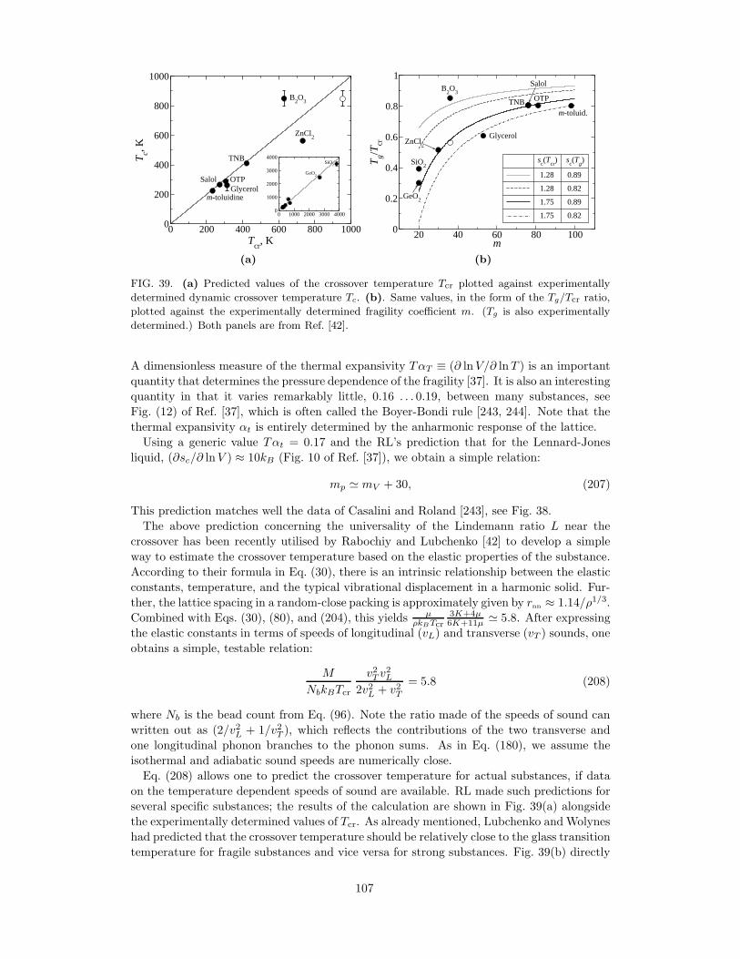
0 200 400 600 800 1000T

cr, K

0

200

400

600

800

1000

Tc, K

ZnCl2

B2O

3

Salol OTP

TNB

Glycerolm-toluidine

0 1000 2000 3000 40000

1000

2000

3000

4000

GeO2

SiO2

(a)

20 40 60 80 100m

0

0.2

0.4

0.6

0.8

1

Tg/T

cr

Glycerol

OTP

m-toluid.

B2O

3

TNB

Salol

SiO2

GeO2

ZnCl2

sc(T

cr) s

c(T

g)

1.28

1.28

1.75

1.75

0.89

0.82

0.89

0.82

(b)

FIG. 39. (a) Predicted values of the crossover temperature Tcr plotted against experimentally

determined dynamic crossover temperature Tc. (b). Same values, in the form of the Tg/Tcr ratio,

plotted against the experimentally determined fragility coefficient m. (Tg is also experimentally

determined.) Both panels are from Ref. [42].

A dimensionless measure of the thermal expansivity TαT ≡ (∂ lnV/∂ lnT ) is an important

quantity that determines the pressure dependence of the fragility [37]. It is also an interesting

quantity in that it varies remarkably little, 0.16 . . . 0.19, between many substances, see

Fig. (12) of Ref. [37], which is often called the Boyer-Bondi rule [243, 244]. Note that the

thermal expansivity αt is entirely determined by the anharmonic response of the lattice.

Using a generic value Tαt = 0.17 and the RL’s prediction that for the Lennard-Jones

liquid, (∂sc/∂ lnV ) ≈ 10kB (Fig. 10 of Ref. [37]), we obtain a simple relation:

mp ≃ mV + 30, (207)

This prediction matches well the data of Casalini and Roland [243], see Fig. 38.

The above prediction concerning the universality of the Lindemann ratio L near the

crossover has been recently utilised by Rabochiy and Lubchenko [42] to develop a simple

way to estimate the crossover temperature based on the elastic properties of the substance.

According to their formula in Eq. (30), there is an intrinsic relationship between the elastic

constants, temperature, and the typical vibrational displacement in a harmonic solid. Fur-

ther, the lattice spacing in a random-close packing is approximately given by rnn ≈ 1.14/ρ1/3.

Combined with Eqs. (30), (80), and (204), this yields µρkBTcr

3K+4µ6K+11µ ≃ 5.8. After expressing

the elastic constants in terms of speeds of longitudinal (vL) and transverse (vT ) sounds, one

obtains a simple, testable relation:

M

NbkBTcr

v2T v2L

2v2L + v2T= 5.8 (208)

where Nb is the bead count from Eq. (96). Note the ratio made of the speeds of sound can

written out as (2/v2L + 1/v2T ), which reflects the contributions of the two transverse and

one longitudinal phonon branches to the phonon sums. As in Eq. (180), we assume the

isothermal and adiabatic sound speeds are numerically close.

Eq. (208) allows one to predict the crossover temperature for actual substances, if data

on the temperature dependent speeds of sound are available. RL made such predictions for

several specific substances; the results of the calculation are shown in Fig. 39(a) alongside

the experimentally determined values of Tcr. As already mentioned, Lubchenko andWolynes

had predicted that the crossover temperature should be relatively close to the glass transition

temperature for fragile substances and vice versa for strong substances. Fig. 39(b) directly

107

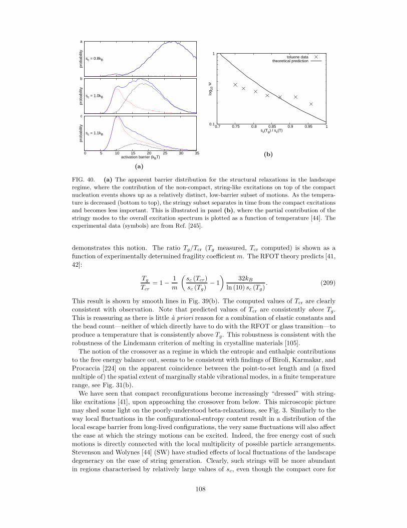
prob

abili

ty

a

sc = 0.8kB

prob

abili

tyb

sc = 1.0kB

0 5 10 15 20 25 30 35

prob

abili

ty

activation barrier (kBT)

c

sc = 1.1kB

(a)

0.1

1

0.7 0.75 0.8 0.85 0.9 0.95 1

log 1

0 Ψ

sc(Tg) / sc(T)

toluene datatheoretical prediction

(b)

FIG. 40. (a) The apparent barrier distribution for the structural relaxations in the landscape

regime, where the contribution of the non-compact, string-like excitations on top of the compact

nucleation events shows up as a relatively distinct, low-barrier subset of motions. As the tempera-

ture is decreased (bottom to top), the stringy subset separates in time from the compact excitations

and becomes less important. This is illustrated in panel (b), where the partial contribution of the

stringy modes to the overall excitation spectrum is plotted as a function of temperature [44]. The

experimental data (symbols) are from Ref. [245].

demonstrates this notion. The ratio Tg/Tcr (Tg measured, Tcr computed) is shown as a

function of experimentally determined fragility coefficientm. The RFOT theory predicts [41,

42]:

TgTcr

= 1− 1

m

(sc (Tcr)

sc (Tg)− 1

)32kB

ln (10) sc (Tg). (209)

This result is shown by smooth lines in Fig. 39(b). The computed values of Tcr are clearly

consistent with observation. Note that predicted values of Tcr are consistently above Tg.

This is reassuring as there is little a priori reason for a combination of elastic constants and

the bead count—neither of which directly have to do with the RFOT or glass transition—to

produce a temperature that is consistently above Tg. This robustness is consistent with the

robustness of the Lindemann criterion of melting in crystalline materials [105].

The notion of the crossover as a regime in which the entropic and enthalpic contributions

to the free energy balance out, seems to be consistent with findings of Biroli, Karmakar, and

Procaccia [224] on the apparent coincidence between the point-to-set length and (a fixed

multiple of) the spatial extent of marginally stable vibrational modes, in a finite temperature

range, see Fig. 31(b).

We have seen that compact reconfigurations become increasingly “dressed” with string-

like excitations [41], upon approaching the crossover from below. This microscopic picture

may shed some light on the poorly-understood beta-relaxations, see Fig. 3. Similarly to the

way local fluctuations in the configurational-entropy content result in a distribution of the

local escape barrier from long-lived configurations, the very same fluctuations will also affect

the ease at which the stringy motions can be excited. Indeed, the free energy cost of such

motions is directly connected with the local multiplicity of possible particle arrangements.

Stevenson and Wolynes [44] (SW) have studied effects of local fluctuations of the landscape

degeneracy on the ease of string generation. Clearly, such strings will be more abundant

in regions characterised by relatively large values of sc, even though the compact core for

108

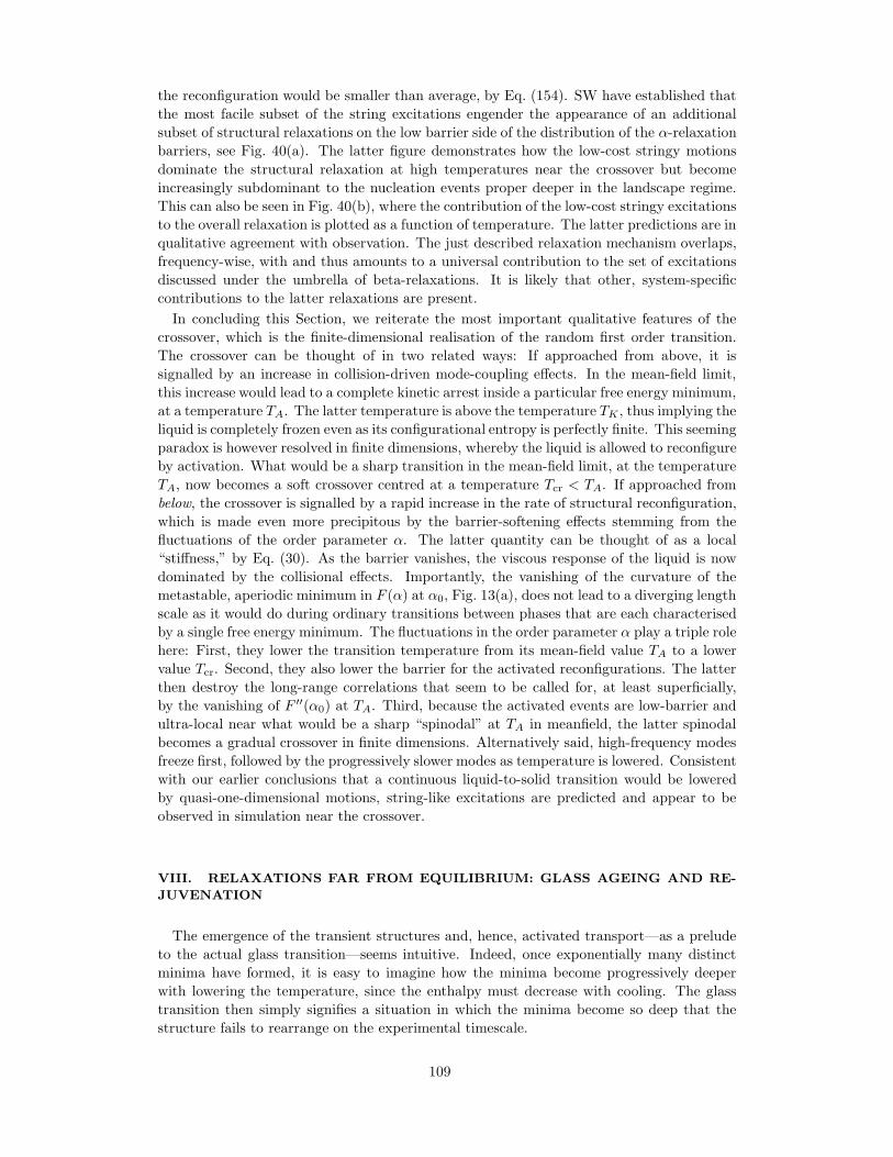
the reconfiguration would be smaller than average, by Eq. (154). SW have established that

the most facile subset of the string excitations engender the appearance of an additional

subset of structural relaxations on the low barrier side of the distribution of the α-relaxation

barriers, see Fig. 40(a). The latter figure demonstrates how the low-cost stringy motions

dominate the structural relaxation at high temperatures near the crossover but become

increasingly subdominant to the nucleation events proper deeper in the landscape regime.

This can also be seen in Fig. 40(b), where the contribution of the low-cost stringy excitations

to the overall relaxation is plotted as a function of temperature. The latter predictions are in

qualitative agreement with observation. The just described relaxation mechanism overlaps,

frequency-wise, with and thus amounts to a universal contribution to the set of excitations

discussed under the umbrella of beta-relaxations. It is likely that other, system-specific

contributions to the latter relaxations are present.

In concluding this Section, we reiterate the most important qualitative features of the

crossover, which is the finite-dimensional realisation of the random first order transition.

The crossover can be thought of in two related ways: If approached from above, it is

signalled by an increase in collision-driven mode-coupling effects. In the mean-field limit,

this increase would lead to a complete kinetic arrest inside a particular free energy minimum,

at a temperature TA. The latter temperature is above the temperature TK , thus implying the

liquid is completely frozen even as its configurational entropy is perfectly finite. This seeming

paradox is however resolved in finite dimensions, whereby the liquid is allowed to reconfigure

by activation. What would be a sharp transition in the mean-field limit, at the temperature

TA, now becomes a soft crossover centred at a temperature Tcr < TA. If approached from

below, the crossover is signalled by a rapid increase in the rate of structural reconfiguration,

which is made even more precipitous by the barrier-softening effects stemming from the

fluctuations of the order parameter α. The latter quantity can be thought of as a local

“stiffness,” by Eq. (30). As the barrier vanishes, the viscous response of the liquid is now

dominated by the collisional effects. Importantly, the vanishing of the curvature of the

metastable, aperiodic minimum in F (α) at α0, Fig. 13(a), does not lead to a diverging length

scale as it would do during ordinary transitions between phases that are each characterised

by a single free energy minimum. The fluctuations in the order parameter α play a triple role

here: First, they lower the transition temperature from its mean-field value TA to a lower

value Tcr. Second, they also lower the barrier for the activated reconfigurations. The latter

then destroy the long-range correlations that seem to be called for, at least superficially,

by the vanishing of F ′′(α0) at TA. Third, because the activated events are low-barrier and

ultra-local near what would be a sharp “spinodal” at TA in meanfield, the latter spinodal

becomes a gradual crossover in finite dimensions. Alternatively said, high-frequency modes

freeze first, followed by the progressively slower modes as temperature is lowered. Consistent

with our earlier conclusions that a continuous liquid-to-solid transition would be lowered

by quasi-one-dimensional motions, string-like excitations are predicted and appear to be

observed in simulation near the crossover.

VIII. RELAXATIONS FAR FROM EQUILIBRIUM: GLASS AGEING AND RE-

JUVENATION

The emergence of the transient structures and, hence, activated transport—as a prelude

to the actual glass transition—seems intuitive. Indeed, once exponentially many distinct

minima have formed, it is easy to imagine how the minima become progressively deeper

with lowering the temperature, since the enthalpy must decrease with cooling. The glass

transition then simply signifies a situation in which the minima become so deep that the

structure fails to rearrange on the experimental timescale.

109

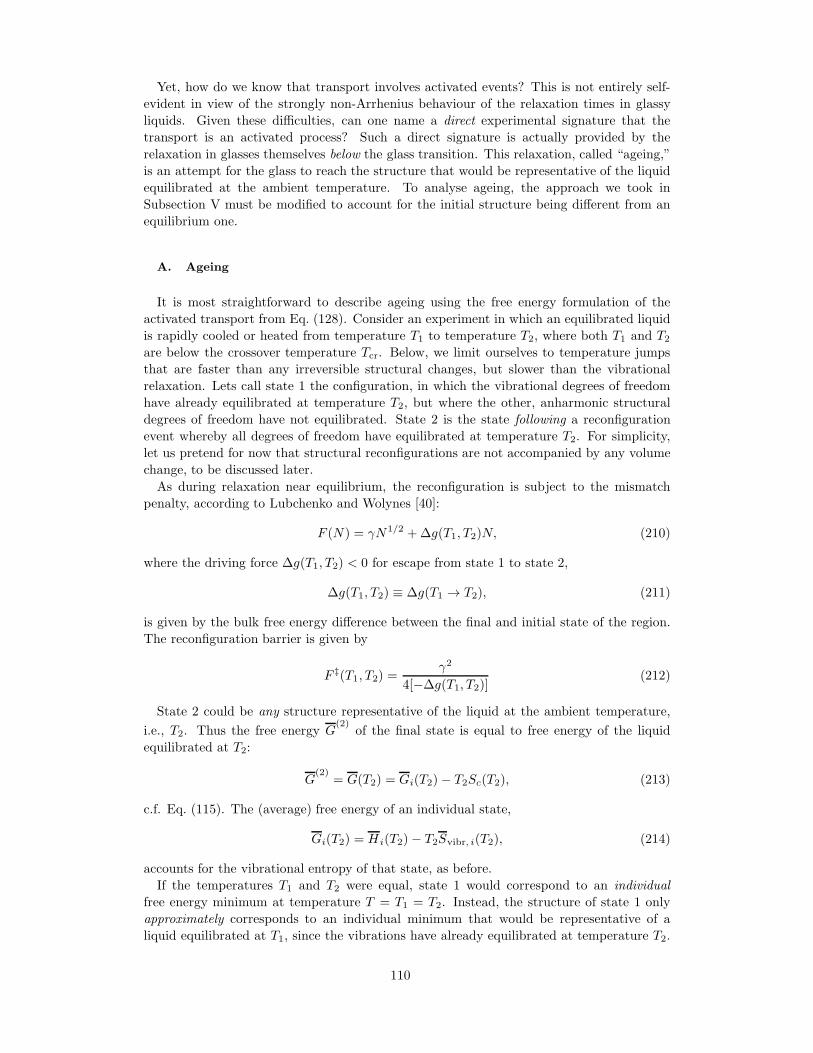
Yet, how do we know that transport involves activated events? This is not entirely self-

evident in view of the strongly non-Arrhenius behaviour of the relaxation times in glassy

liquids. Given these difficulties, can one name a direct experimental signature that the

transport is an activated process? Such a direct signature is actually provided by the

relaxation in glasses themselves below the glass transition. This relaxation, called “ageing,”

is an attempt for the glass to reach the structure that would be representative of the liquid

equilibrated at the ambient temperature. To analyse ageing, the approach we took in

Subsection V must be modified to account for the initial structure being different from an

equilibrium one.

A. Ageing

It is most straightforward to describe ageing using the free energy formulation of the

activated transport from Eq. (128). Consider an experiment in which an equilibrated liquid

is rapidly cooled or heated from temperature T1 to temperature T2, where both T1 and T2are below the crossover temperature Tcr. Below, we limit ourselves to temperature jumps

that are faster than any irreversible structural changes, but slower than the vibrational

relaxation. Lets call state 1 the configuration, in which the vibrational degrees of freedom

have already equilibrated at temperature T2, but where the other, anharmonic structural

degrees of freedom have not equilibrated. State 2 is the state following a reconfiguration

event whereby all degrees of freedom have equilibrated at temperature T2. For simplicity,

let us pretend for now that structural reconfigurations are not accompanied by any volume

change, to be discussed later.

As during relaxation near equilibrium, the reconfiguration is subject to the mismatch

penalty, according to Lubchenko and Wolynes [40]:

F (N) = γN1/2 +∆g(T1, T2)N, (210)

where the driving force ∆g(T1, T2) < 0 for escape from state 1 to state 2,

∆g(T1, T2) ≡ ∆g(T1 → T2), (211)

is given by the bulk free energy difference between the final and initial state of the region.

The reconfiguration barrier is given by

F ‡(T1, T2) =γ2

4[−∆g(T1, T2)](212)

State 2 could be any structure representative of the liquid at the ambient temperature,

i.e., T2. Thus the free energy G(2)

of the final state is equal to free energy of the liquid

equilibrated at T2:

G(2)

= G(T2) = Gi(T2)− T2Sc(T2), (213)

c.f. Eq. (115). The (average) free energy of an individual state,

Gi(T2) = Hi(T2)− T2Svibr, i(T2), (214)

accounts for the vibrational entropy of that state, as before.

If the temperatures T1 and T2 were equal, state 1 would correspond to an individual

free energy minimum at temperature T = T1 = T2. Instead, the structure of state 1 only

approximately corresponds to an individual minimum that would be representative of a

liquid equilibrated at T1, since the vibrations have already equilibrated at temperature T2.

110

The vibrations at T1 and T2 are of different magnitude, if T1 6= T2, and so some shift in

the average position of the particles is expected upon vibrational relaxation, owing to the

anharmonicity of the lattice. Still, the structure in state 1 is completely isomorphic to the

structure at T1. We will thus assume approximately that the configuration—and hence the

enthalpy—of state 1 are the same as in equilibrium at temperature T1. On the other hand,

the vibrational entropy in state 1 is approximately equal to the equilibrium vibrational

entropy at temperature T2:

G(1) ≈ Hi(T1)− T2Svibr, i(T2). (215)

Thus the bulk driving force ∆g for reconfiguration, per particle, is given by [40]:

∆g(T1, T2) = g(2) − g(1) ≈ h(T2)− h(T1)− T2sc(T2). (216)

Using Eq. (95), one obtains an explicit expression for the driving force:

−∆g(T1, T2) = ∆cp(Tg)Tg

[(T2TK

− 1

)− ln

(T2T1

)]. (217)

We now specifically focus on downward temperature quenches, T2 < T1. Given the

postulated quickness of the quench, we must identify T1 as the glass transition temperature:

T1 = Tg, while T2 is the ambient temperature T . Under these circumstances, h(T ) −h(Tg) =

∫ T

Tg∆cpdT < 0. Thus, the driving force for the escape from the structure quenched

at Tg, at the still lower temperature temperature T < Tg, exceeds the driving force for

reconfigurations in a liquid equilibrated at the ambient temperature T :

−∆g(Tg, T ) > −∆g(T, T ), if T < Tg. (218)

It is easy to see that the activation barrier for ageing is only weakly temperature depen-

dent [40]. Indeed, at T = Tg, ∆g = −∆cp(Tg)(Tg/TK−1). The most stable aperiodic struc-

ture corresponds to the putative ideal-glass state that would be equilibrium at the Kauz-

mann temperature TK , where sc = 0. Hereby, the driving force is ∆g = h(TK) − h(Tg) =

−∆cp(Tg) ln(Tg/TK). To decide on the temperature dependence of the mismatch penalty,

if any, we revisit to Eq. (142), in which the energy prefactor h now consists of the contri-

bution from the free energy fluctuations on the inside, δGi(T2), and that on the outside

δ[Hi(T1) − T2Svibr(T2)]. According to Eq. (158), γ ∝ [K(T1 + T2)/ρ]1/2, considering that

the bulk modulus and density barely change with temperature in the frozen glass. Thus the

reconfiguration barrier goes as (2Tg)2/(Tg/TK−1) and (Tg+TK)2/ ln(Tg/TK) at Tg and TK

respectively. The two quantities differ by at most 25%, since empirically, the ratio Tg/TK is

numerically at most 2 (for very strong substances), but is usually considerably less than 2.

Because the activation barrier is only weakly temperature dependent below Tg, the ap-

parent activation energy (not the free energy!)

Eact =∂(F ‡/kBT )

∂(1/T ), (219)

which is generally not equal to F ‡, is predicted to exhibit a discontinuous jump following

a rapid quench, c.f. Fig. 3. (The activation free energy is continuous through the glass

transition.) A convenient framework for quantitative discussion of this jump is provided

by the Narayanaswamy-Moynihan-Tool formalism [246–248], in which the relaxation rate

in quenched glasses is phenomenologically decomposed into a purely activated part and a

temperature-independent part reflecting a fictive temperature Tf :

kn.e. = k0 exp

−xNMT

Eact, eq

kBT− (1− xNMT)

Eact, eq

kBTf.

, (220)

111

0 0.2 0.4 0.6 0.8 1

x

0

50

100

150

200

250

300

m

B2O3

PVC

PS

As2Se3

PVAc

NMT

(a)

Tg

Tg

Tg Tg

Tg

Tg

TgTgTg

Tg

Tg

TgTg

TgT

T

(b)

FIG. 41. (a) Smooth line: The RFOT-predicted, simple relation between the NMT coefficient x,

which reflects the discontinuity of the apparent activation rate (219) and the fragility. Symbols: Ex-

perimental data. Note experimental data show significant scatter even for the same substance. (b)

After a considerable period of ageing well below Tg a patchwork of equilibrated and non-equilibrated

mosaic cells will be found, leading to a distribution of fictive temperatures and emergence of ultra-

slow relaxations. After Ref. [40]

Here Eact, eq is the apparent activation barrier from Eq. (219) in an equilibrated liquid,

i.e., just above the glass transition: Eact, eq = Eact(T+g ). The fictive temperature Tf is an

approximate concept. By construction, it is chosen so that the structure equilibrated at Tfwould be as similar as possible to the actual structure. Above Tg, Tf = T , of course. Below

Tg, one often adopts Tf = Tg since the structure of the frozen glass is quite similar to that

of the liquid at the glass transition, apart from some ageing and subtle changes stemming

from differences in the vibrational amplitude, which is an anharmonic effect. For the NMT

description to be internally-consistent, one must disregard the temperature dependence of

the activation barrier below Tg, which we have seen is a good approximation. This implies

F ‡|T<Tg ≈ F ‡(Tg, TK) leading to ∂(F ‡/kBT )/∂(1/T )|T<Tg = F ‡(Tg, TK), where F ‡(T1, T2)is from Eq. (212). Finally, the quantity xNMT, 0 < xNMT < 1, is a dimensionless measure of

the decrease in the apparent activation energy. Thus, xMNTEact, eq = F ‡(Tg, TK) ⇒ x−1MNT

=

Eact, eq/F‡(Tg, TK). Further using Eqs. (173), (212), and (217), this straightforwardly leads

to the following estimate [40]:

x−1MNT

= m

(log10 e)

F ‡(Tg)

kBTg

[γ(TK)

γ(Tg)

]2(Tg/TK − 1)

ln(Tg/TK)

−1

, (221)

where m stands for the fragility coefficient m from Eq. (173). The last ratio on the r.h.s.

depends on the Tg/TK ratio only weakly, as already remarked. Using a specific, generic value

Tg/TK = 1.3 and ignoring the temperature dependence of the coefficient γ, one obtains a

simpler yet relation between the fragility coefficient and the discontinuity of the apparent

activation energy at the glass transition [40]:

m ≃ 19

xNMT

. (222)

This simple relation agrees well with experiment, see Fig. 41(a), thus supporting the RFOT-

advanced microscopic picture on a very basic level.

We shall now discuss the effects of volume mismatch during ageing. The expression for the

driving force in Eq. (216) corresponds to a process at constant pressure and thus is applicable

112

for relatively shallow quenches. For considerable T -jumps, however, the situation is more

complicated since on the timescale of the nucleation event, the sample is a mechanically

stable solid with a non-zero shear modulus. And so, insofar as the equilibrium thermal

expansivity αeq ≡ (1/V )(∂V/∂T )p exceeds the (largely vibrational) expansivity of a frozen

glass αvibr, downward T -jumps will be accompanied by some stretching of the environment:

A compact region of the material is essentially replaced by a region with a smaller volume,

following an ageing event. The expansivity of an equilibrated liquid usually does significantly

exceed that of the corresponding glass, see for instance Ref. [249]. Despite this circumstance,

the effects of volume mismatch between the aged and unrelaxed glass do not significantly

affect the ageing rate, as we discuss in detail in Appendix A.

After a considerable period of ageing well below Tg, a patchwork of equilibrated and non-

equilibrated mosaic cells will develop [40], see Fig. 41(b). If the equilibrium energy at T is

further than a standard deviation from the typical energy at Tg, the distribution of energies

will be noticeably bimodal and the idea of a single fictive temperature will break down. The

typical magnitude of temperature fluctuations is given by (kBT2/∆cvN

∗)1/2 [55]. Thus,

significant deviations from a unimodal distribution of fictive temperatures are not expected

if ∆T = Tg − T < (kBT2/∆cvN

∗)1/2 ≡ δT ∗. For Tg relevant to 1 hr. quenches this gives

δT ∗/Tg ≃ 0.07. Most of the Alegria et al. [250] data lie in this modest quenching range,

while “hyperquenched” samples (with ∆T ≫ δT ∗) will often fall outside the allowed range

of using a single fictive temperature. When a sample has a two-peaked distribution of local

energies, the RFOT theory predicts an ultra-slow component of relaxation will arise. Notice

that an equilibrated region at the temperature T = Tg − δT ∗ will relax on the tens to

hundreds of hours scale, if τg is taken to be one hour. (The relaxation barrier depends on

temperature only weakly.)

B. Rejuvenation

Let us now switch focus to upward temperature jumps, T2 > T1, which is a different

type of ageing experiment. In this type of ageing, the structure locally escapes from being

relatively deep in the free energy landscape to the region in the phase space where the free

energy minima are relatively shallow, by Eqs. (170) and (159). Consistent with this notion,

Eq. (217) prescribes that there is not as much driving force for structural relaxation when

T2 > T1 than in equilibrium at temperature T = T1 = T2:

−∆g(T1, T2) < −∆g(T2, T2), if T2 > T1, (223)

c.f. Eq. (218). For this reason, the process of glass rejuvenation—i.e., warming up and

subsequent equilibration of a vitrified sample at the target temperature—is slower than the

relaxation time in equilibrium at that same temperature. On the other hand, the relaxation

barrier for a T2 > T1 process is lower than the relaxation barrier in equilibrium at T1, as

follows from Eq. (217) (note T1 > TK of course):

−∆g(T1, T2) > −∆g(T1, T1), if T2 > T1. (224)

Thus the sample will undergo irreversible relaxation to configurations typical of equilibrium

at temperature T2, following the temperature jump. Furthermore, due to the relatively high

mobility on the edge, to be discussed in Section X, the sample will not melt uniformly but

will begin melting preferentially from the edge where it is being heated. Once a region

is melted, a mobility front will propagate in the sample since the melted regions relax

significantly faster than the those regions not reached by the front. It is convenient to

113

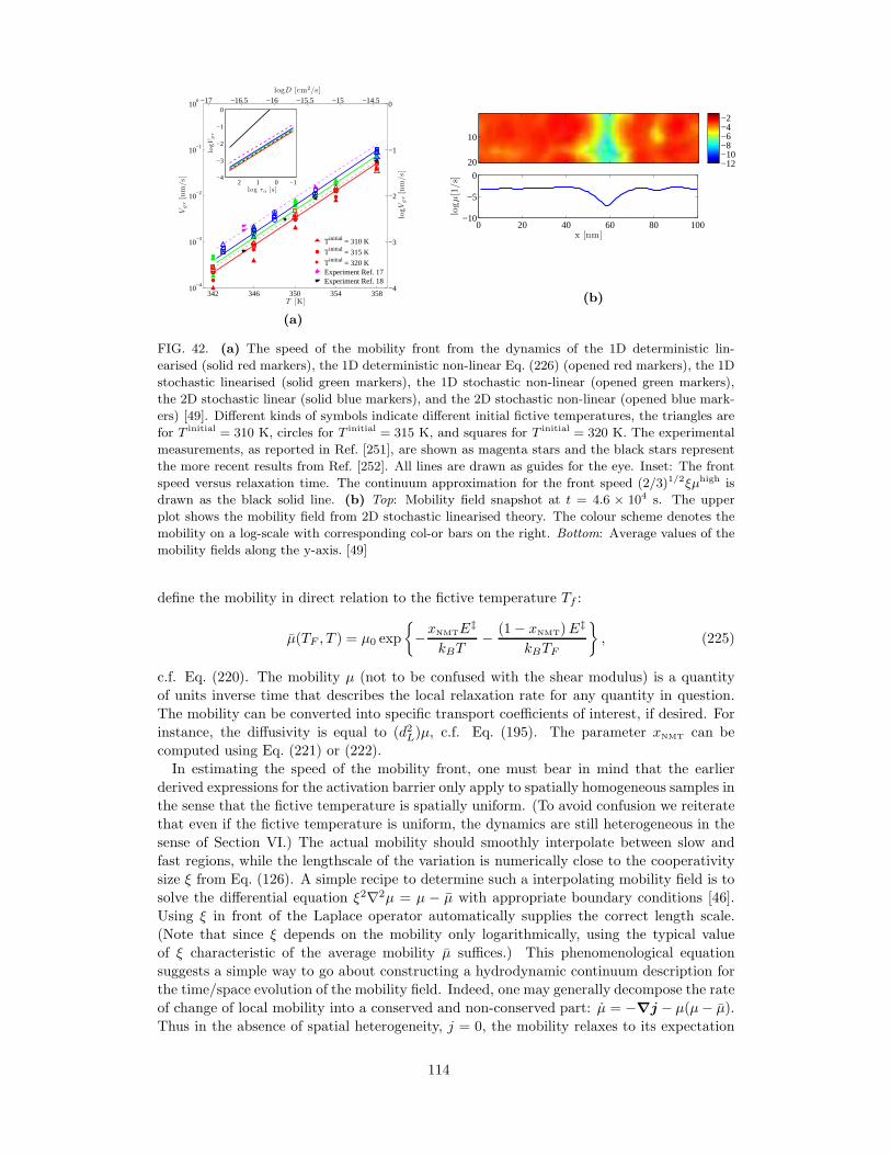
342 346 350 354 35810

−4

10−3

10−2

10−1

100

T [K]

Vg

r[n

m/s]

Tinitial = 310 K

Tinitial = 315 K

Tinitial = 320 KExperiment Ref. 17Experiment Ref. 18

−17 −16.5 −16 −15.5 −15 −14.5

−4

−3

−2

−1

0

logD [cm2/s]

logV

gr

[nm

/s]

−1012−4

−3

−2

−1

0

log τα [s ]

logV

gr

(a)

10

20 −12−10−8−6−4−2

0 20 40 60 80 100−10

−5

0

x [nm]

logµ[1/s]

(b)

FIG. 42. (a) The speed of the mobility front from the dynamics of the 1D deterministic lin-

earised (solid red markers), the 1D deterministic non-linear Eq. (226) (opened red markers), the 1D

stochastic linearised (solid green markers), the 1D stochastic non-linear (opened green markers),

the 2D stochastic linear (solid blue markers), and the 2D stochastic non-linear (opened blue mark-

ers) [49]. Different kinds of symbols indicate different initial fictive temperatures, the triangles are

for T initial = 310 K, circles for T initial = 315 K, and squares for T initial = 320 K. The experimental

measurements, as reported in Ref. [251], are shown as magenta stars and the black stars represent

the more recent results from Ref. [252]. All lines are drawn as guides for the eye. Inset: The front

speed versus relaxation time. The continuum approximation for the front speed (2/3)1/2ξµhigh is

drawn as the black solid line. (b) Top: Mobility field snapshot at t = 4.6 × 104 s. The upper

plot shows the mobility field from 2D stochastic linearised theory. The colour scheme denotes the

mobility on a log-scale with corresponding col-or bars on the right. Bottom: Average values of the

mobility fields along the y-axis. [49]

define the mobility in direct relation to the fictive temperature Tf :

µ(TF , T ) = µ0 exp

−xNMTE

‡

kBT− (1− xNMT)E

‡

kBTF

, (225)

c.f. Eq. (220). The mobility µ (not to be confused with the shear modulus) is a quantity

of units inverse time that describes the local relaxation rate for any quantity in question.

The mobility can be converted into specific transport coefficients of interest, if desired. For

instance, the diffusivity is equal to (d2L)µ, c.f. Eq. (195). The parameter xNMT can be

computed using Eq. (221) or (222).

In estimating the speed of the mobility front, one must bear in mind that the earlier

derived expressions for the activation barrier only apply to spatially homogeneous samples in

the sense that the fictive temperature is spatially uniform. (To avoid confusion we reiterate

that even if the fictive temperature is uniform, the dynamics are still heterogeneous in the

sense of Section VI.) The actual mobility should smoothly interpolate between slow and

fast regions, while the lengthscale of the variation is numerically close to the cooperativity

size ξ from Eq. (126). A simple recipe to determine such a interpolating mobility field is to

solve the differential equation ξ2∇2µ = µ − µ with appropriate boundary conditions [46].

Using ξ in front of the Laplace operator automatically supplies the correct length scale.

(Note that since ξ depends on the mobility only logarithmically, using the typical value

of ξ characteristic of the average mobility µ suffices.) This phenomenological equation

suggests a simple way to go about constructing a hydrodynamic continuum description for

the time/space evolution of the mobility field. Indeed, one may generally decompose the rate

of change of local mobility into a conserved and non-conserved part: µ = −∇j − µ(µ− µ).

Thus in the absence of spatial heterogeneity, j = 0, the mobility relaxes to its expectation

114

value µ with the local relaxation rate, which is equal to the mobility itself. Likewise, the

flux j can be connected to the magnitude of spatial variation in µ via a Fick-like law:

j = −ξ2µ∇µ. Putting these notions together yields the following transport equation [49]:

µ = ∇(µ ξ2∇µ

)− µ (µ− µ) + δg +∇δj, (226)

where we have also included two terms corresponding to thermal noise, ∇δj and δg, for

the conserved and non-conserved part of the mobility relaxation rate respectively. The

magnitude of these random-noise terms can be fixed using the fluctuation-dissipation the-

orem [49]. The linearised version of the above equation is easy to write down: µ =

∇(µ ξ2∇µ

)− µ (µ− µ) + δg + ∇δj. Note either this or the original non-linear equation

(226) automatically insure that the mobility varies on the length scale ξ. The simplest way

to quantify the approach of the local fictive temperature to the ambient temperature is

through the following, ultralocal relaxation law

TF = −µ (TF − T ) + δη, (227)

where δη is the corresponding noise-term. Note the fictive temperature is a structural

variable that has no dynamics of its own other than through the mobility transport; thus

there is no diffusive term on the r.h.s. of Eq. (227).

Aside from the mobility-dependent “diffusivity,” Eq. (226) is the celebrated Fisher-

Kolmogorov-Petrovsky-Piscounov [253, 254] equation that can be used to study migration

of organisms, as accompanied by death and procreation, and has also been used to model

flame propagation. This equation (in 1D) also governs the generating function for the den-

sity distribution in the random directed-polymer problem; curiously, it exhibits a singularity

intimately related to the glass transition in the random energy model [255].

In Fig. 42(a), we show the results of the solution of Eq. (226)—together with Eq. (227)—

and its linearised version. The solutions in the presence and absence of the noise-terms,

called “stochastic” and “deterministic” respectively, are illustrated. One observes good

agreement of the predictions with the experimentally observed mobility front propagation.

A snapshot of the linearised, stochastic simulation in 2D is provided in Fig. 42(b).

Note that a reasonable approximation for the speed of the mobility front can be obtained

without actually solving the differential equations above, by using an analogy with flame

fronts [48]. According to this approximation, shown by the black solid line in the inset of

Fig. 42(a), the front speed is a fixed fraction of the mobility µhigh in the sample equilibrated

at the ambient temperature, viz., (2/3)1/2ξµhigh. While an overestimation, this simple result

matches observation qualitatively.

IX. RHEOLOGICAL AND MECHANICAL ANOMALIES

A. Shear thinning

We have already seen that the microscopic picture advanced by the RFOT theory can

be used to estimate on a microscopic basis the viscosity, which is the key quantity in the

science of rheology. Next we shall see how the very same picture allows one to answer

an interesting puzzle in the rheology of silicate melts. These melts exhibit pronounced

deviations from the Newtonian liquid response, in the form of shear thinning, at shear rates

that are, universally, about three orders of magnitude lower than the inverse relaxation time

〈τ〉−1. Shear thinning means the viscous response from from Eq. (197) is sublinear in the

velocity gradient ∂vi/∂xj , implying an apparent viscosity that decreases with ∂vi/∂xj , see

Fig. 43(a). Viscosity measurements can be imagined in a simple geometry in which two

115

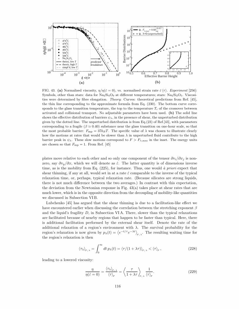
10-4

10-3

10-2

10-1

100

ε. <τ>10

-2

10-1

100

η/η(

ε. =0)

predictedbreakdown

474oC

479oC

482oC

493oC

504oC

506oC

Na2Si

2O

5theory, low Ttheory, high Tsimpl’d, low T

(a)

0.5 0.6 0.7 0.8 0.9 1.0Effective Barrier Height

10-3

10-2

10-1

100

101

102

103

Bar

rier

Dis

trib

utio

ns

ψ, Fλ,max= 0.8F

mp

(λ=0)

ψ, λ=0 (unperturbed)

0.5 0.6 0.7 0.8 0.9 1

Fλ0.5

0.6

0.7

0.8

0.9

1F

(b)

FIG. 43. (a) Normalised viscosity, η/η(ε = 0), vs. normalised strain rate ε 〈τ 〉. Experiment [256]:

Symbols, other than stars: data for Na2Si4O9 at different temperatures; stars: Na2Si2O5. Viscosi-

ties were determined by fibre elongation. Theory: Curves: theoretical predictions from Ref. [45],

the thin line corresponding to the approximate formula from Eq. (230). The bottom curve corre-

sponds to the glass transition temperature, the top to the temperature Tc of the crossover between

activated and collisional transport. No adjustable parameters have been used. (b) The solid line

shows the effective distribution of barriers ψλ, in the presence of shear, the unperturbed distribution

given by the dotted line. The unperturbed distribution is from Eq.(23) of Ref.[43], with parameters

corresponding to a fragile (β ≃ 0.40) substance near the glass transition on one-hour scale, so that

the most probable barrier: Fmp = 37kBT . The specific value of λ was chosen to illustrate clearly

how the motions at rates that would be slower than λ in unperturbed fluid contribute to the high

barrier peak in ψλ. These slow motions correspond to F > Fλ,max in the inset. The energy units

are chosen so that Fmp = 1. From Ref. [45]

plates move relative to each other and so only one component of the tensor ∂vi/∂xj is non-

zero, say ∂vy/∂x, which we will denote as ε. The latter quantity is of dimensions inverse

time, as is the mobility from Eq. (225), for instance. Thus, one would a priori expect that

shear thinning, if any at all, would set in at a rate ε comparable to the inverse of the typical

relaxation time, or, perhaps, typical relaxation rate. (Because silicates are strong liquids,

there is not much difference between the two averages.) In contrast with this expectation,

the deviation from the Newtonian response in Fig. 43(a) takes place at shear rates that are

much lower, which is in the opposite direction from the decoupling of mobility-like quantities

we discussed in Subsection VIB.

Lubchenko [45] has argued that the shear thinning is due to a facilitation-like effect we

have encountered earlier when discussing the correlation between the stretching exponent β

and the liquid’s fragility D, in Subsection VIA. There, slower than the typical relaxations

are facilitated because of nearby regions that happen to be faster than typical. Here, there

is additional facilitation performed by the external shear itself. Denote the rate of the

additional relaxation of a region’s environment with λ. The survival probability for the

region’s relaxation is now given by pλ(t) =⟨e−t/τe−λt

⟩F , λ

. The resulting waiting time for

the region’s relaxation is then

〈τλ〉F , λ =

∫ ∞

0

dt pλ(t) = 〈τ/(1 + λτ)〉F , λ < 〈τ〉

F, (228)

leading to a lowered viscosity:

η

η(ε = 0)=

〈τλ〉F , λ

〈τ〉F

=

⟨τ

1 + λτ

⟩

F , λ

1

〈τ〉F

. (229)

116

The rate λ can be self-consistently determined [45] at a given value of experimentally

imposed shear rate, by energy conservation: The energy flow through the domain boundary,

due to the external shear, must match the rate of energy dissipation in the sample bulk,

due to the shear. It turns out that both at relatively high and low shear rate, λ and ε

are proportional to each other while the proportionality constant only differs by a factor

of two between the two extremes. Thus a simple approximate expression for the relation

between the quantities can be written down, which does not depend on the detailed barrier

distribution:

λ ≈ [1.5√2(a/dL)(ξ/a)

3/2] ε. (230)

This equation indicates that the facilitation rate λ, as sensed by an individual reconfiguring

region, is significantly enhanced compared to the experimentally imposed rate ε. The en-

hancement is, in almost equal measure, is due to the smallness of individual displacements

dL from Eq. (127) and to the size of the cooperative region, which is about (ξ/a)3 ≃ 102

near Tg. The numerical factor in the square brackets in Eq. (230) is thus about 103 near

Tg. Conversely, this enhancement implies that externally imposed shear at rate as low as

10−3τ−1 will significantly increase the effective relaxation rate of a region.

The theoretical prediction for the shear thinning, corresponding to the simple form (230)

and to a more accurate relation are shown in Fig. 43(a), alongside with experimental

data [256]. The agreement between theory and experiment is very good; note that no

adjustable parameters were used. The degree of shear thinning is predicted not to depend

sensitively on the width of the barrier distribution.

The argument in Ref. [45] self-consistently predicts the magnitude of the shear rate at

which the proposed picture breaks down. In this picture, the external shear does not signifi-

cantly modify the mechanism of the relaxation itself but, instead, sets a non-zero lower limit

on the relaxation rate λ. At the same time, this rate λ may not exceed the intrinsic rate at

which the interface of an individual region relaxes, which can be estimated geometrically.

One can think of a region roughly as being in the centre of a cube made of 3 × 3 × 3 = 27

cooperative regions. Thus the boundary of the region will relax, on average, once per time

(〈τ〉 /27) or so. If forced to relax at a higher rate, the boundary must relax via other means,

such as bond breaking. This would occur at viscosities indicated by the horizontal arrow in

Fig. 43(a). This estimate is quite consistent with the shear rate at which the glassy fibres

broke, whose elongation was employed to measure the shear thinning.

Note that the shear-driven decrease in relaxation times, Eq. (228), implies lower effective

barriers, by virtue of Eq.(132):

Fλ ≡ F − kBT ln[1 + e(F−Fλ,max)/kBT

], (231)

where Fλ,max is the highest possible effective barrier for a fixed λ:

Fλ,max ≡ −kBT ln(λτ0), (232)

see the inset of Fig. 43(b). It is straightforward to show that the distribution ψλ of the

shear-modified barriers from Eq. (231) is related to the unperturbed barrier distribution ψ

according to:

ψλ(Fλ) = ψ(F )[1 + e(F−Fλ,max)/kBT

], (233)

where F is understood as a function of Fλ via Eq.(231). Both the unperturbed and shear-

modified barrier distributions (for a fragile substance near the glass transition) are shown

in Fig.43 for a particular value of λ. We thus directly observe how facilitation modifies the

barrier distribution. Presumably, one may use a similar approach to determine the barrier

117

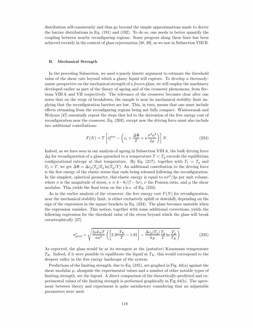
distribution self-consistently and thus go beyond the simple approximations made to derive

the barrier distributions in Eq. (191) and (192). To do so, one needs to better quantify the

coupling between nearby reconfiguring regions. Some progress along these lines has been

achieved recently in the context of glass rejuvenation [48, 49], as we saw in Subsection VIII B.

B. Mechanical Strength

In the preceding Subsection, we used a purely kinetic argument to estimate the threshold

value of the shear rate beyond which a glassy liquid will rupture. To develop a thermody-

namic perspective on the mechanical strength of a frozen glass, we will employ the machinery

developed earlier as part of the theory of ageing and of the crossover phenomena, from Sec-

tions VIII A and VII respectively. The relevance of the crossover becomes clear after one

notes that on the verge of breakdown, the sample is near its mechanical stability limit im-

plying that the reconfiguration barriers are low. This, in turn, means that one must include

effects stemming from the reconfiguring regions being not fully compact. Wisitsorasak and

Wolynes [47] essentially repeat the steps that led to the derivation of the free energy cost of

reconfiguration near the crossover, Eq. (203), except now the driving force must also include

two additional contributions:

F (N) = T

[spercc −

(sc +

∆Φ

T+ κ

σ2a3

2µ

)]N. (234)

Indeed, as we have seen in our analysis of ageing in Subsection VIII A, the bulk driving force

∆g for reconfiguration of a glass quenched to a temperature T < Tg exceeds the equilibrium

configurational entropy at that temperature. By Eq. (217), together with T1 = Tg and

T2 = T , we get ∆Φ = ∆cp(Tg)Tg ln(Tg/T ). An additional contribution to the driving force

is the free energy of the elastic stress that ends being released following the reconfiguration.

In the simplest, spherical geometry, this elastic energy is equal to κσ2/2µ per unit volume,

where σ is the magnitude of stress, κ ≡ 3− 6/(7− 5ν), ν the Poisson ratio, and µ the shear

modulus. This yields the final term on the r.h.s. of Eq. (234).

As in the earlier analysis of the crossover, the free energy cost F (N) for reconfiguration,

near the mechanical stability limit, is either exclusively uphill or downhill, depending on the

sign of the expression in the square brackets in Eq. (234). The glass becomes unstable when

the expression vanishes. This notion, together with some additional corrections, yields the

following expression for the threshold value of the stress beyond which the glass will break

catastrophically [47]:

σ∗pred =

√2µkBT

κa3

([3.20

TKT

− 1.91

]− ∆cp(Tg)

kB

TgT

lnTgTK

)(235)

As expected, the glass would be at its strongest at the (putative) Kauzmann temperature

TK . Indeed, if it were possible to equilibrate the liquid at TK , this would correspond to the

deepest valley in the free energy landscape of the system.

Predictions of the limiting strength, due to Eq. (235), are graphed in Fig. 44(a) against the

shear modulus µ, alongside the experimental values and a number of other notable types of

limiting strength, see the legend. A direct comparison of the theoretically-predicted and ex-

perimental values of the limiting strength is performed graphically in Fig.44(b). The agree-

ment between theory and experiment is quite satisfactory considering that no adjustable

parameters were used.

118

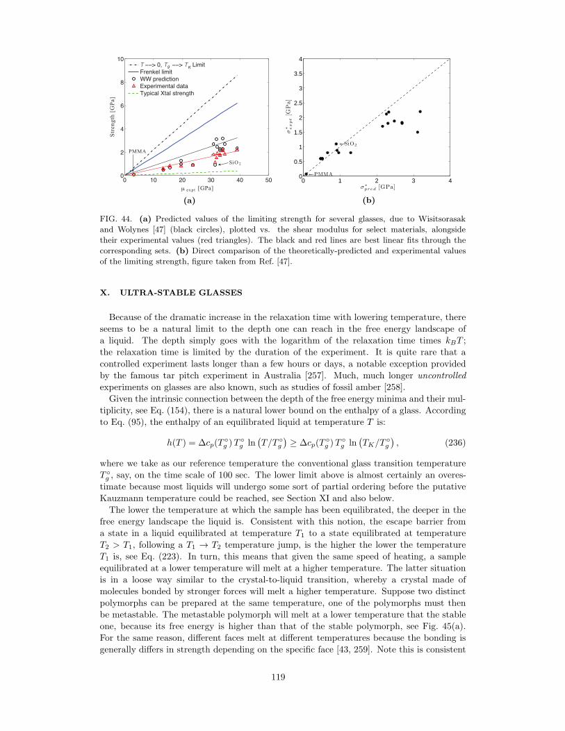
0 10 20 30 40 500

2

4

6

8

10

PMMA

SiO 2

μ exp t [GPa]

Str

en

gth

[G

Pa]

T −−> 0, T −−> T LimitFrenkel limitWW predictionExperimental dataTypical Xtal strength

Kg

(a)

0 1 2 3 40

0.5

1

1.5

2

2.5

3

3.5

4

←− PMMA

←− SiO2

σ∗ ex

pt

[GP

a]

σ ∗pred [GPa]

(b)

FIG. 44. (a) Predicted values of the limiting strength for several glasses, due to Wisitsorasak

and Wolynes [47] (black circles), plotted vs. the shear modulus for select materials, alongside

their experimental values (red triangles). The black and red lines are best linear fits through the

corresponding sets. (b) Direct comparison of the theoretically-predicted and experimental values

of the limiting strength, figure taken from Ref. [47].

X. ULTRA-STABLE GLASSES

Because of the dramatic increase in the relaxation time with lowering temperature, there

seems to be a natural limit to the depth one can reach in the free energy landscape of

a liquid. The depth simply goes with the logarithm of the relaxation time times kBT ;

the relaxation time is limited by the duration of the experiment. It is quite rare that a

controlled experiment lasts longer than a few hours or days, a notable exception provided

by the famous tar pitch experiment in Australia [257]. Much, much longer uncontrolled

experiments on glasses are also known, such as studies of fossil amber [258].

Given the intrinsic connection between the depth of the free energy minima and their mul-

tiplicity, see Eq. (154), there is a natural lower bound on the enthalpy of a glass. According

to Eq. (95), the enthalpy of an equilibrated liquid at temperature T is:

h(T ) = ∆cp(Tg )T

g ln

(T/T

g

)≥ ∆cp(T

g )T

g ln

(TK/T

g

), (236)

where we take as our reference temperature the conventional glass transition temperature

T g , say, on the time scale of 100 sec. The lower limit above is almost certainly an overes-

timate because most liquids will undergo some sort of partial ordering before the putative

Kauzmann temperature could be reached, see Section XI and also below.

The lower the temperature at which the sample has been equilibrated, the deeper in the

free energy landscape the liquid is. Consistent with this notion, the escape barrier from

a state in a liquid equilibrated at temperature T1 to a state equilibrated at temperature

T2 > T1, following a T1 → T2 temperature jump, is the higher the lower the temperature

T1 is, see Eq. (223). In turn, this means that given the same speed of heating, a sample

equilibrated at a lower temperature will melt at a higher temperature. The latter situation

is in a loose way similar to the crystal-to-liquid transition, whereby a crystal made of

molecules bonded by stronger forces will melt a higher temperature. Suppose two distinct

polymorphs can be prepared at the same temperature, one of the polymorphs must then

be metastable. The metastable polymorph will melt at a lower temperature that the stable

one, because its free energy is higher than that of the stable polymorph, see Fig. 45(a).

For the same reason, different faces melt at different temperatures because the bonding is

generally differs in strength depending on the specific face [43, 259]. Note this is consistent

119

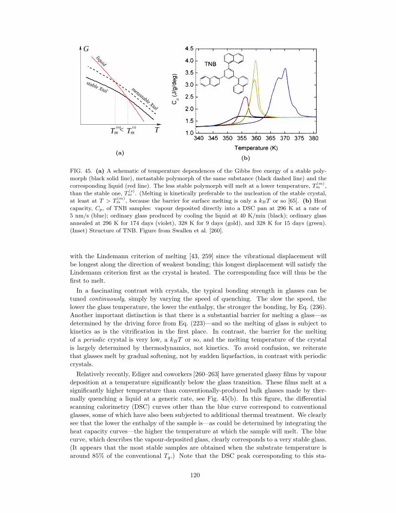
liquid

(m)

mT < mT T

G

metastable Xtal

stable Xtal

(s)

(a)(b)

FIG. 45. (a) A schematic of temperature dependences of the Gibbs free energy of a stable poly-

morph (black solid line), metastable polymorph of the same substance (black dashed line) and the

corresponding liquid (red line). The less stable polymorph will melt at a lower temperature, T(m)m ,

than the stable one, T(s)m . (Melting is kinetically preferable to the nucleation of the stable crystal,

at least at T > T(m)m , because the barrier for surface melting is only a kBT or so [65]. (b) Heat

capacity, Cp, of TNB samples: vapour deposited directly into a DSC pan at 296 K at a rate of

5 nm/s (blue); ordinary glass produced by cooling the liquid at 40 K/min (black); ordinary glass

annealed at 296 K for 174 days (violet), 328 K for 9 days (gold), and 328 K for 15 days (green).

(Inset) Structure of TNB. Figure from Swallen et al. [260].

with the Lindemann criterion of melting [43, 259] since the vibrational displacement will

be longest along the direction of weakest bonding; this longest displacement will satisfy the

Lindemann criterion first as the crystal is heated. The corresponding face will thus be the

first to melt.

In a fascinating contrast with crystals, the typical bonding strength in glasses can be

tuned continuously, simply by varying the speed of quenching. The slow the speed, the

lower the glass temperature, the lower the enthalpy, the stronger the bonding, by Eq. (236).

Another important distinction is that there is a substantial barrier for melting a glass—as

determined by the driving force from Eq. (223)—and so the melting of glass is subject to

kinetics as is the vitrification in the first place. In contrast, the barrier for the melting

of a periodic crystal is very low, a kBT or so, and the melting temperature of the crystal

is largely determined by thermodynamics, not kinetics. To avoid confusion, we reiterate

that glasses melt by gradual softening, not by sudden liquefaction, in contrast with periodic

crystals.

Relatively recently, Ediger and coworkers [260–263] have generated glassy films by vapour

deposition at a temperature significantly below the glass transition. These films melt at a

significantly higher temperature than conventionally-produced bulk glasses made by ther-

mally quenching a liquid at a generic rate, see Fig. 45(b). In this figure, the differential

scanning calorimetry (DSC) curves other than the blue curve correspond to conventional

glasses, some of which have also been subjected to additional thermal treatment. We clearly

see that the lower the enthalpy of the sample is—as could be determined by integrating the

heat capacity curves—the higher the temperature at which the sample will melt. The blue

curve, which describes the vapour-deposited glass, clearly corresponds to a very stable glass.

(It appears that the most stable samples are obtained when the substrate temperature is

around 85% of the conventional Tg.) Note that the DSC peak corresponding to this sta-

120

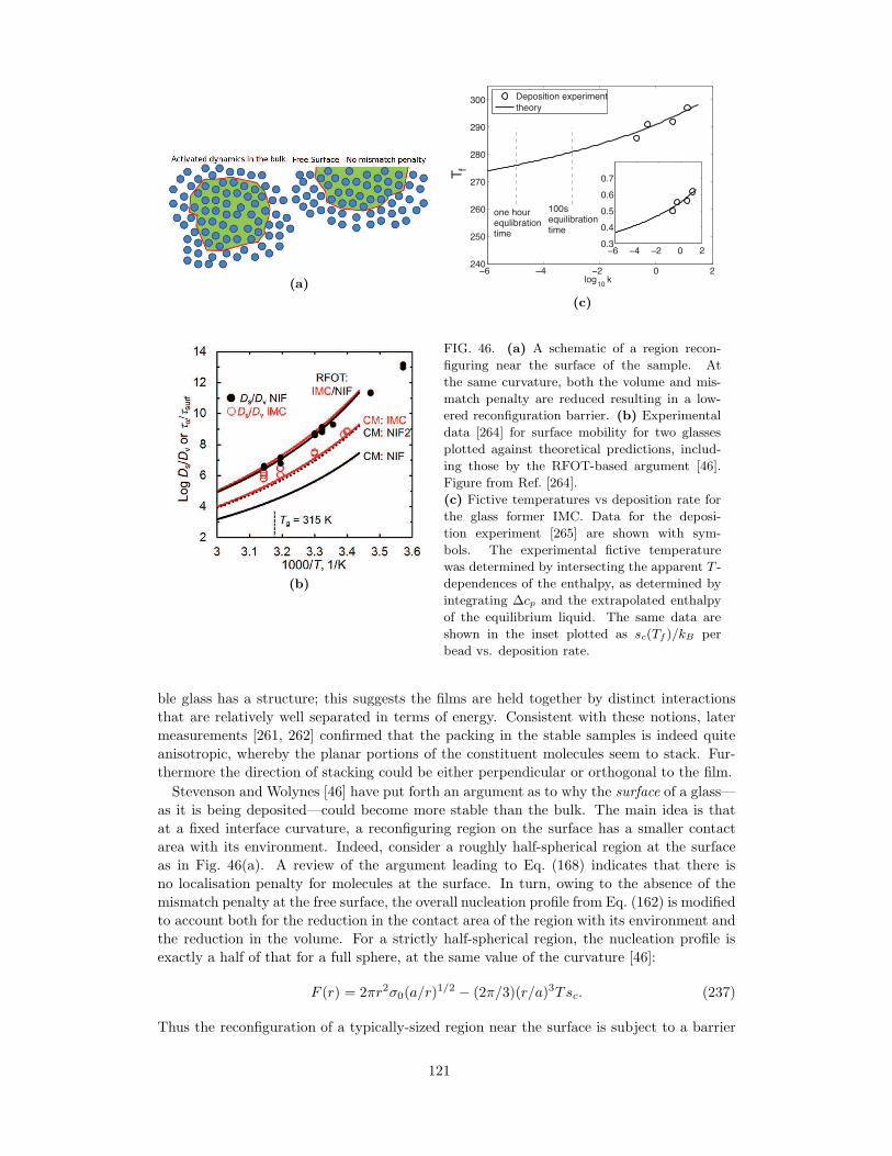
(a)

(b)

−6 −4 −2 0 2240

250

260

270

280

290

300

log10

k

Tf

−6 −4 −2 0 20.3

0.4

0.5

0.6

0.7

Deposition experiment

theory

one hourequlibrationtime

100sequilibrationtime

(c)

FIG. 46. (a) A schematic of a region recon-

figuring near the surface of the sample. At

the same curvature, both the volume and mis-

match penalty are reduced resulting in a low-

ered reconfiguration barrier. (b) Experimental

data [264] for surface mobility for two glasses

plotted against theoretical predictions, includ-

ing those by the RFOT-based argument [46].

Figure from Ref. [264].

(c) Fictive temperatures vs deposition rate for

the glass former IMC. Data for the deposi-

tion experiment [265] are shown with sym-

bols. The experimental fictive temperature

was determined by intersecting the apparent T -

dependences of the enthalpy, as determined by

integrating ∆cp and the extrapolated enthalpy

of the equilibrium liquid. The same data are

shown in the inset plotted as sc(Tf )/kB per

bead vs. deposition rate.

ble glass has a structure; this suggests the films are held together by distinct interactions

that are relatively well separated in terms of energy. Consistent with these notions, later

measurements [261, 262] confirmed that the packing in the stable samples is indeed quite

anisotropic, whereby the planar portions of the constituent molecules seem to stack. Fur-

thermore the direction of stacking could be either perpendicular or orthogonal to the film.

Stevenson and Wolynes [46] have put forth an argument as to why the surface of a glass—

as it is being deposited—could become more stable than the bulk. The main idea is that

at a fixed interface curvature, a reconfiguring region on the surface has a smaller contact

area with its environment. Indeed, consider a roughly half-spherical region at the surface

as in Fig. 46(a). A review of the argument leading to Eq. (168) indicates that there is

no localisation penalty for molecules at the surface. In turn, owing to the absence of the

mismatch penalty at the free surface, the overall nucleation profile from Eq. (162) is modified

to account both for the reduction in the contact area of the region with its environment and

the reduction in the volume. For a strictly half-spherical region, the nucleation profile is

exactly a half of that for a full sphere, at the same value of the curvature [46]:

F (r) = 2πr2σ0(a/r)1/2 − (2π/3)(r/a)3Tsc. (237)

Thus the reconfiguration of a typically-sized region near the surface is subject to a barrier

121

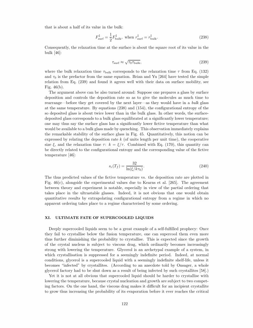
that is about a half of its value in the bulk:

F ‡surf =

1

2F ‡bulk, when r

‡surf = r‡bulk. (238)

Consequently, the relaxation time at the surface is about the square root of its value in the

bulk [46]:

τsurf ≈√τ0τbulk, (239)

where the bulk relaxation time τbulk corresponds to the relaxation time τ from Eq. (132)

and τ0 is the prefactor from the same equation. Brian and Yu [264] have tested the simple

relation from Eq. (239) and found it agrees well with their data on surface mobility, see

Fig. 46(b).

The argument above can be also turned around: Suppose one prepares a glass by surface

deposition and controls the deposition rate so as to give the molecules as much time to

rearrange—before they get covered by the next layer—as they would have in a bulk glass

at the same temperature. By equations (238) and (154), the configurational entropy of the

so deposited glass is about twice lower than in the bulk glass. In other words, the surface-

deposited glass corresponds to a bulk glass equilibrated at a significantly lower temperature;

one may thus say the surface glass has a significantly lower fictive temperature than what

would be available to a bulk glass made by quenching. This observation immediately explains

the remarkable stability of the surface glass in Fig. 45. Quantitatively, this notion can be

expressed by relating the deposition rate k (of units length per unit time), the cooperative

size ξ, and the relaxation time τ : k = ξ/τ . Combined with Eq. (170), this quantity can

be directly related to the configurational entropy and the corresponding value of the fictive

temperature [46]:

sc(Tf ) =32

ln(ξ/kτ0). (240)

The thus predicted values of the fictive temperature vs. the deposition rate are plotted in

Fig. 46(c), alongside the experimental values due to Kearns et al. [265]. The agreement

between theory and experiment is notable, especially in view of the partial ordering that

takes place in the ultrastable glasses. Indeed, it is not obvious that one would obtain

quantitative results by extrapolating configurational entropy from a regime in which no

apparent ordering takes place to a regime characterised by some ordering.

XI. ULTIMATE FATE OF SUPERCOOLED LIQUIDS

Deeply supercooled liquids seem to be a great example of a self-fulfilled prophecy: Once

they fail to crystallise below the fusion temperature, one can supercool them even more

thus further diminishing the probability to crystallise. This is expected since the growth

of the crystal nucleus is subject to viscous drag, which ordinarily becomes increasingly

strong with lowering the temperature. Glycerol is an archetypal example of a system, in

which crystallisation is suppressed for a seemingly indefinite period. Indeed, at normal

conditions, glycerol is a supercooled liquid with a seemingly indefinite shelf-life, unless it

becomes “infected” by crystallites. (According to an anecdote told by Onsager, a whole

glycerol factory had to be shut down as a result of being infected by such crystallites [58].)

Yet it is not at all obvious that supercooled liquid should be harder to crystallise with

lowering the temperature, because crystal nucleation and growth are subject to two compet-

ing factors. On the one hand, the viscous drag makes it difficult for an incipient crystallite

to grow thus increasing the probability of its evaporation before it ever reaches the critical

122

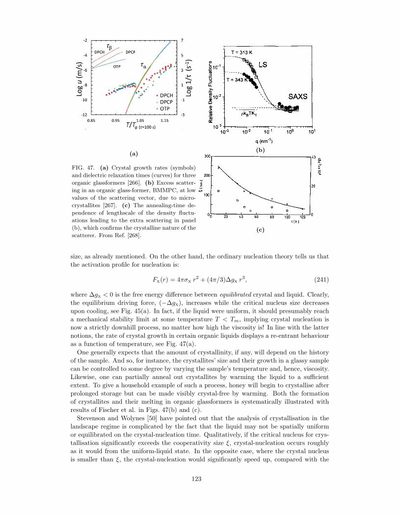
(a)

FIG. 47. (a) Crystal growth rates (symbols)

and dielectric relaxation times (curves) for three

organic glassformers [266]. (b) Excess scatter-

ing in an organic glass-former, BMMPC, at low

values of the scattering vector, due to micro-

crystallites [267]. (c) The annealing-time de-

pendence of lengthscale of the density fluctu-

ations leading to the extra scattering in panel

(b), which confirms the crystalline nature of the

scatterer. From Ref. [268].

(b)

(c)

size, as already mentioned. On the other hand, the ordinary nucleation theory tells us that

the activation profile for nucleation is:

FX(r) = 4πσX r2 + (4π/3)∆gX r

3, (241)

where ∆gX < 0 is the free energy difference between equilibrated crystal and liquid. Clearly,

the equilibrium driving force, (−∆gX), increases while the critical nucleus size decreases

upon cooling, see Fig. 45(a). In fact, if the liquid were uniform, it should presumably reach

a mechanical stability limit at some temperature T < Tm, implying crystal nucleation is

now a strictly downhill process, no matter how high the viscosity is! In line with the latter

notions, the rate of crystal growth in certain organic liquids displays a re-entrant behaviour

as a function of temperature, see Fig. 47(a).

One generally expects that the amount of crystallinity, if any, will depend on the history

of the sample. And so, for instance, the crystallites’ size and their growth in a glassy sample

can be controlled to some degree by varying the sample’s temperature and, hence, viscosity.

Likewise, one can partially anneal out crystallites by warming the liquid to a sufficient

extent. To give a household example of such a process, honey will begin to crystallise after

prolonged storage but can be made visibly crystal-free by warming. Both the formation

of crystallites and their melting in organic glassformers is systematically illustrated with

results of Fischer et al. in Figs. 47(b) and (c).

Stevenson and Wolynes [50] have pointed out that the analysis of crystallisation in the

landscape regime is complicated by the fact that the liquid may not be spatially uniform

or equilibrated on the crystal-nucleation time. Qualitatively, if the critical nucleus for crys-

tallisation significantly exceeds the cooperativity size ξ, crystal-nucleation occurs roughly

as it would from the uniform-liquid state. In the opposite case, where the crystal nucleus

is smaller than ξ, the crystal-nucleation would significantly speed up, compared with the

123

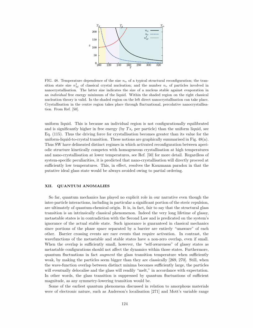
FIG. 48. Temperature dependence of the size nα of a typical structural reconfiguration; the tran-

sition state size n‡

M of classical crystal nucleation; and the number nν of particles involved in

nanocrystallisation. The latter size indicates the size of a nucleus stable against evaporation in

an individual free energy minimum of the liquid. Within the shaded region on the right classical

nucleation theory is valid. In the shaded region on the left direct nanocrystallisation can take place.

Crystallisation in the centre region takes place through fluctuational, percolative nanocrystallisa-

tion. From Ref. [50].

uniform liquid. This is because an individual region is not configurationally equilibrated

and is significantly higher in free energy (by Tsc per particle) than the uniform liquid, see

Eq. (115). Thus the driving force for crystallisation becomes greater than its value for the

uniform-liquid-to-crystal transition. These notions are graphically summarised in Fig. 48(a).

Thus SW have delineated distinct regimes in which activated reconfiguration between aperi-

odic structure kinetically competes with homogeneous crystallisation at high temperatures

and nano-crystallisation at lower temperatures, see Ref. [50] for more detail. Regardless of

system-specific peculiarities, it is predicted that nano-crystallisation will directly proceed at

sufficiently low temperatures. This, in effect, resolves the Kauzmann paradox in that the

putative ideal glass state would be always avoided owing to partial ordering.

XII. QUANTUM ANOMALIES

So far, quantum mechanics has played no explicit role in our narrative even though the

inter-particle interactions, including in particular a significant portion of the steric repulsion,

are ultimately of quantum-chemical origin. It is, in fact, fair to say that the structural glass

transition is an intrinsically classical phenomenon. Indeed the very long lifetime of glassy,

metastable states is in contradiction with the Second Law and is predicated on the system’s

ignorance of the actual stable state. Such ignorance is guaranteed in classical mechanics

since portions of the phase space separated by a barrier are entirely “unaware” of each

other. Barrier crossing events are rare events that require activation. In contrast, the

wavefunctions of the metastable and stable states have a non-zero overlap, even if small.

When the overlap is sufficiently small, however, the “self-awareness” of glassy states as

metastable configurations should not affect the dynamics within those states. Furthermore,

quantum fluctuations in fact augment the glass transition temperature when sufficiently

weak, by making the particles seem bigger than they are classically [269, 270]. Still, when

the wave-function overlap between distinct minima becomes sufficiently large, the particles

will eventually delocalise and the glass will readily “melt,” in accordance with expectation.

In other words, the glass transition is suppressed by quantum fluctuations of sufficient

magnitude, as any symmetry-lowering transition would be.

Some of the earliest quantum phenomena discussed in relation to amorphous materials

were of electronic nature, such as Anderson’s localisation [271] and Mott’s variable range

124

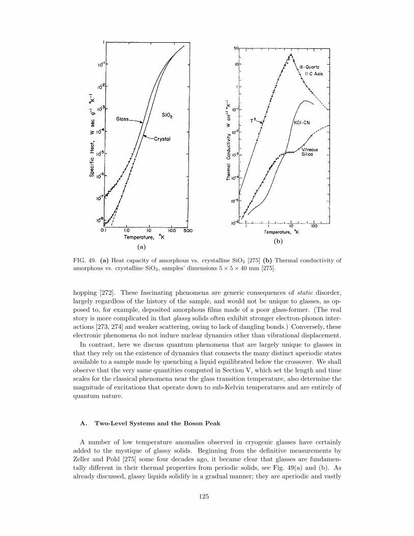
(a)(b)

FIG. 49. (a) Heat capacity of amorphous vs. crystalline SiO2 [275] (b) Thermal conductivity of

amorphous vs. crystalline SiO2, samples’ dimensions 5 × 5 × 40 mm [275].

hopping [272]. These fascinating phenomena are generic consequences of static disorder,

largely regardless of the history of the sample, and would not be unique to glasses, as op-

posed to, for example, deposited amorphous films made of a poor glass-former. (The real

story is more complicated in that glassy solids often exhibit stronger electron-phonon inter-

actions [273, 274] and weaker scattering, owing to lack of dangling bonds.) Conversely, these

electronic phenomena do not induce nuclear dynamics other than vibrational displacement.

In contrast, here we discuss quantum phenomena that are largely unique to glasses in

that they rely on the existence of dynamics that connects the many distinct aperiodic states

available to a sample made by quenching a liquid equilibrated below the crossover. We shall

observe that the very same quantities computed in Section V, which set the length and time

scales for the classical phenomena near the glass transition temperature, also determine the

magnitude of excitations that operate down to sub-Kelvin temperatures and are entirely of

quantum nature.

A. Two-Level Systems and the Boson Peak

A number of low temperature anomalies observed in cryogenic glasses have certainly

added to the mystique of glassy solids. Beginning from the definitive measurements by

Zeller and Pohl [275] some four decades ago, it became clear that glasses are fundamen-

tally different in their thermal properties from periodic solids, see Fig. 49(a) and (b). As

already discussed, glassy liquids solidify in a gradual manner; they are aperiodic and vastly

125

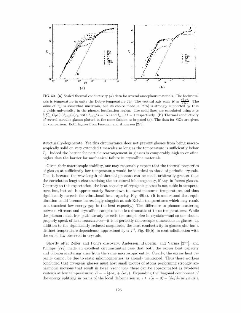
(a) (b)

FIG. 50. (a) Scaled thermal conductivity (κ) data for several amorphous materials. The horizontal

axis is temperature in units the Debye temperature TD. The vertical axis scale K ≡k3BT2

Dπ~cs

. The

value of TD is somewhat uncertain, but its choice made in [276] is strongly supported by that

it yields universality in the phonon localisation region. The solid lines are calculated using κ ≃13

∑ω Cph(ω)lmfp(ω)cS with lmfp/λ = 150 and lmfp/λ = 1 respectively. (b) Thermal conductivity

of several metallic glasses plotted in the same fashion as in panel (a). The data for SiO2 are given

for comparison. Both figures from Freeman and Anderson [276].

structurally-degenerate. Yet this circumstance does not prevent glasses from being macro-

scopically solid on very extended timescales so long as the temperature is sufficiently below

Tg. Indeed the barrier for particle rearrangement in glasses is comparably high to or often

higher that the barrier for mechanical failure in crystalline materials.

Given their macroscopic stability, one may reasonably expect that the thermal properties

of glasses at sufficiently low temperatures would be identical to those of periodic crystals.

This is because the wavelength of thermal phonons can be made arbitrarily greater than

the correlation length characterising the structural inhomogeneity, if any, in frozen glasses.

Contrary to this expectation, the heat capacity of cryogenic glasses is not cubic in tempera-

ture, but, instead, is approximately linear down to lowest measured temperatures and thus

significantly exceeds the vibrational heat capacity, Fig. 49(a). (It is understood that equi-

libration could become increasingly sluggish at sub-Kelvin temperatures which may result

in a transient low energy gap in the heat capacity.) The difference in phonon scattering

between vitreous and crystalline samples is no less dramatic at these temperatures: While

the phonon mean free path already exceeds the sample size in crystals—and so one should

properly speak of heat conductance—it is of perfectly microscopic dimensions in glasses. In

addition to the significantly reduced magnitude, the heat conductivity in glasses also has a

distinct temperature dependence, approximately ∝ T 2, Fig. 49(b), in contradistinction with

the cubic law observed in crystals.

Shortly after Zeller and Pohl’s discovery, Anderson, Halperin, and Varma [277], and

Phillips [278] made an excellent circumstantial case that both the excess heat capacity

and phonon scattering arise from the same microscopic entity. Clearly, the excess heat ca-

pacity cannot be due to static inhomogeneities, as already mentioned. Thus those workers

concluded that cryogenic glasses must host small groups of atoms performing strongly an-

harmonic motions that result in local resonances; these can be approximated as two-level

systems at low temperatures: E = − 12 (ǫσz +∆σx). Expanding the diagonal component of

the energy splitting in terms of the local deformation u, ǫ ≈ ǫ(u = 0) + (∂ǫ/∂u)u yields a

126

coupling to the sound waves: g ≡ − 12 (∂ǫ/∂u), thus yielding the TLS energy function:

E = −1

2(ǫσz +∆σx) + guσz. (242)

A flat density of states, n(E) = P = const, approximately accounts for the T -dependence

of both the heat capacity and conductivity [277–279]. Phonon-echo and single-molecule

spectroscopy have directly confirmed the resonant nature of these mysterious excitations

and even captured their becoming multi-level at increasing temperatures [280–282].

Already Zeller and Pohl noted the heat conductivity—a dimensional quantity—seemed

only mildly system-dependent, a point that was forcefully brought home by Freeman and

Anderson [276] some 15 years later, see Fig. 50(a). The latter authors have shown the ratio

of the phonon mean-free path λmfp to the thermal phonon wavelength λth is near universally

≈ 150 for all tested, insulating vitreous substances, some polymeric. This ratio can be also

expressed in terms of the parameters of the two level systems:

lmfp

λth=

(P g2

ρmc2s

)−1

≃ 150, (243)

where ρm and cs are the mass density and speed of sound respectively. One way to interpret

the above figure is to say that the vibrational plain waves—or phonons—are reasonably well-

defined, wave-like quasi-particles, despite the aperiodicity of the lattice. In addition to the

low-T regime in Fig. 50(a), which corresponds to the near universal line lmfp/λth ≃ 150, there

is also the regime on the higher temperature flank on Fig. 50(a), where this ratio is about one:

lmfp/λth ≃ 1. This regime is often referred to as the Ioffe-Regel regime [272, 283], whereby

the phonon is no longer a well-defined quasi-particle. Instead, it is more appropriate to speak

of energy transport in the solid as hopping of vibrational packets, a picture originally (and

incorrectly) envisioned by Einstein for crystalline solids [284]. The intermediate regime 1 <

lmfp/λth < 150 is of considerable interest, too: This region corresponds with a significant rise

in the heat capacity, Fig. 52(a), often called the heat-capacity “bump,” but also an increased

rate of phonon scattering, which leads to a “plateau” in the heat conductivity, 101 . T/θ .

102 in Fig. 50(a). One should not fail to notice that the plateau temperatures correspond to

terahertz frequencies and thus match, frequency-wise, the Boson Peak excitations in Fig. 3.

Yu and Leggett [285] (YL) have stressed that there is little a priori reason for the ratio

from Eq. (243) to be so consistent between different substances, considering that the density

of states P varies by at least two orders of magnitude. (The magnitude of the variation,

while considerable, is still surprisingly small given the chemical variation among the tested

materials.) YL also noted that the phonon-mediated interaction between two TLSs goes

as (g2/ρmc2s)r

−3—a fact we have already encountered at the end of Subsection IVD—

consistent with Eq. (243) and the fact that P has dimensions inverse energy-volume. Based

on this realisation and noting the long-range character of the 1/r3 interaction, YL proposed

that the apparent density of states P pertains to some renormalised excitations which span a

large number of the local resonances. Thus this density of states could be a universal quotient

of the inverse of the elemental interaction (g2/ρmc2s)

−1 irrespective of the precise nature of

those local resonances. Showing why this quotient should be of order 102 has been difficult,

but the “interaction” scenario is still being pursued [286–288]. To avoid confusion with the

Bevzenko-Lubchenko model [154, 155], we note that in the latter, the interaction is very

strong, comparable to the glass transition temperature, Fig. 22(b), whereas the interaction

between the apparent two-level systems is closer to sub-Kelvin energy scales [289], see also

below.

Local resonances naturally arise in the RFOT scenario of the glass transition. Hereby

the near universality of the ratio in Eq. (243) can be traced to the near universality in

the cooperativity size ξ. To see this we first note that the activated reconfigurations in a

127

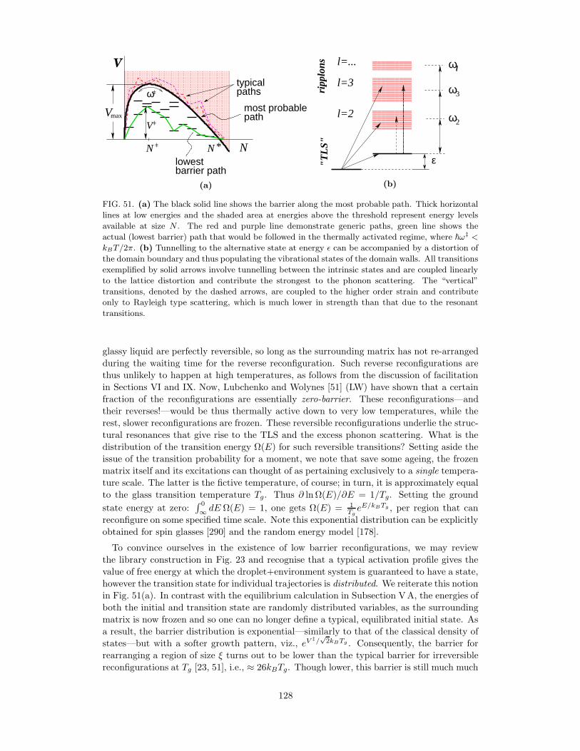
ω

N *N

V

lowestbarrier path

typicalpaths

most probablepathmaxV

V

N

(a)

ω3

ω2

ωl

ε

l=2

l=3

l=...

ripp

lons

"TL

S"

(b)

FIG. 51. (a) The black solid line shows the barrier along the most probable path. Thick horizontal

lines at low energies and the shaded area at energies above the threshold represent energy levels

available at size N . The red and purple line demonstrate generic paths, green line shows the

actual (lowest barrier) path that would be followed in the thermally activated regime, where ~ω‡ <

kBT/2π. (b) Tunnelling to the alternative state at energy ǫ can be accompanied by a distortion of

the domain boundary and thus populating the vibrational states of the domain walls. All transitions

exemplified by solid arrows involve tunnelling between the intrinsic states and are coupled linearly

to the lattice distortion and contribute the strongest to the phonon scattering. The “vertical”

transitions, denoted by the dashed arrows, are coupled to the higher order strain and contribute

only to Rayleigh type scattering, which is much lower in strength than that due to the resonant

transitions.

glassy liquid are perfectly reversible, so long as the surrounding matrix has not re-arranged

during the waiting time for the reverse reconfiguration. Such reverse reconfigurations are

thus unlikely to happen at high temperatures, as follows from the discussion of facilitation

in Sections VI and IX. Now, Lubchenko and Wolynes [51] (LW) have shown that a certain

fraction of the reconfigurations are essentially zero-barrier. These reconfigurations—and

their reverses!—would be thus thermally active down to very low temperatures, while the

rest, slower reconfigurations are frozen. These reversible reconfigurations underlie the struc-

tural resonances that give rise to the TLS and the excess phonon scattering. What is the

distribution of the transition energy Ω(E) for such reversible transitions? Setting aside the

issue of the transition probability for a moment, we note that save some ageing, the frozen

matrix itself and its excitations can thought of as pertaining exclusively to a single tempera-

ture scale. The latter is the fictive temperature, of course; in turn, it is approximately equal

to the glass transition temperature Tg. Thus ∂ lnΩ(E)/∂E = 1/Tg. Setting the ground

state energy at zero:∫ 0

∞ dE Ω(E) = 1, one gets Ω(E) = 1TgeE/kBTg , per region that can

reconfigure on some specified time scale. Note this exponential distribution can be explicitly

obtained for spin glasses [290] and the random energy model [178].

To convince ourselves in the existence of low barrier reconfigurations, we may review

the library construction in Fig. 23 and recognise that a typical activation profile gives the

value of free energy at which the droplet+environment system is guaranteed to have a state,

however the transition state for individual trajectories is distributed. We reiterate this notion

in Fig. 51(a). In contrast with the equilibrium calculation in Subsection VA, the energies of

both the initial and transition state are randomly distributed variables, as the surrounding

matrix is now frozen and so one can no longer define a typical, equilibrated initial state. As

a result, the barrier distribution is exponential—similarly to that of the classical density of

states—but with a softer growth pattern, viz., eV‡/

√2kBTg . Consequently, the barrier for

rearranging a region of size ξ turns out to be lower than the typical barrier for irreversible

reconfigurations at Tg [23, 51], i.e., ≈ 26kBTg. Though lower, this barrier is still much much

128

higher than what could be tunnelled through, however. Conversely, the chances that a

region of size ξ will have a zero reconfiguration barrier, e−26kBTg/√2kBTg ∼ 10−8, are small,

even if not astronomically small. LW go further and consider the set of trajectories available

to regions larger than ξ. To a region of size N > N∗, there are esc(N−N∗)/kB more states

available. And so given sc(Tg) = 0.82, at (N −N∗) = 22—only a 10% increase relative to

N∗(Tg)—one can in fact find a trajectory with a zero barrier, since esc(N−N∗)/kB ∼ 108.

Importantly, alternative configurations are kinetically accessible only to regions larger than

N∗(Tg). The energy of such a larger region is below that of the typically reconfiguring region

at Tg, implying only the negative tail of the distribution Ω(E) = (1/Tg)eE/kBTg is kinetically

accessible, by tunnelling. That the barrier is zero makes the question of the tunnelling mass

moot. Still, LW [51] point out the tunnelling coordinate is surprisingly low mass, in apparent

similarity to the domain-wall solution in the Su-Schrieffer-Heeger hamiltonian [291]. (This

similarity will be prominent in Subsection XIIB.) We thus conclude that the density of

states of the resonances that would thermally active at very low temperature is [22, 23, 51]:

n(ǫ) ≃ 1

Tgξ3e−|ǫ|/kBTg . (244)

The resulting density of low energy excitations, ǫ≪ kBTg, is thus

P = 1/Tgξ3. (245)

Interestingly, it is determined by the characteristics of the solid that were set at the tem-

perature of preparation, which is two orders of magnitude greater than the ambient, cryo-

genic temperature! The generic value of P is about 1045 J−1m−3, consistent with observa-

tion [292]. It is easy to see that he TLS density of states should decrease with lowering of the

glass transition temperature and, hence, of the rate of quench during vitrification. Indeed,

by Eqs. (160) and (165), we obtain P ∝ s2c and P ∝ s2c/T respectively. Either quantity is

an increasing function of temperature, because sc ∝ (T − TK). We thus conclude that for a

material in the landscape regime, the density of states of the TLS should be the lower the

more stable the glass is. Generically, this means that denser glasses have fewer two-level

systems.

Let us return to a previous notion that near the crossover, the free energy cost of particle

localisation is comparable to that due to elastic deformation of the newly formed elastic con-

tinuum. The latter free energy is fixed by the equipartition theorem: 〈|gu|〉 ≃ ρmc2sa

3⟨u2⟩≃

kBTcr, where ρm is the mass density. (This simple estimate is consistent with a more detailed

argument [51].) Thus we may estimate the TLS-phonon coupling in Eq. (242):

g ≃√ρmc2sa

3kBTg. (246)

Eqs. (245) and (246) immediately yield that the mysterious universality in the phonon

scattering, as expressed in the ratio from Eq. (243) stems from the near universality of the

cooperative size near the preparation temperature of the sample:

lmfp

λth=

(P g2

ρmc2s

)−1

≃(ξ(Tg)

a

)3

≃ 102. (247)

According to the prediction above, the slower the quench used to prepare the glass, the less

intense phonon scattering will be at cryogenic temperatures. This is consistent with our ear-

lier statement that glasses residing in deeper free energy minima are bonded more strongly.

Conversely, glasses made by quicker quenches should exhibit more phonon scattering. The

latter notion, however, applies only so long as the material remains in the landscape regime.

For instance, we have seen that amorphous films prepared by vapour deposition on a cold

129

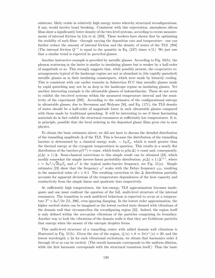
substrate, likely reside in relatively high energy states whereby structural reconfigurations,

if any, would involve bond breaking. Consistent with this expectation, amorphous silicon

films show a significantly lower density of the two-level systems, according to recent measure-

ments of internal friction by Liu et al. [293]. These workers have shown that by optimising

the stability of such films—through varying the deposition rate and temperature—one can

further reduce the amount of internal friction and the density of states of the TLS. [294]

(The internal friction Q−1 is equal to the quantity in Eq. (247) times π/2.) We just saw

that a similar trend is expected in quenched glasses.

Another instructive example is provided by metallic glasses. According to Fig. 50(b), the

phonon scattering in the latter is similar to insulating glasses but is weaker by a half-order

of magnitude or so. This strongly suggests that, while possibly present, the cooperative re-

arrangements typical of the landscape regime are not as abundant in (the rapidly quenched)

metallic glasses as in their insulating counterparts, which were made by leisurely cooling.

This is consistent with our earlier remarks in Subsection IVC that metallic glasses made

by rapid quenching may not be as deep in the landscape regime as insulating glasses. Yet

another interesting example is the ultrastable glasses of indomethacine. These do not seem

to exhibit the two-level systems within the measured temperature interval and the sensi-

tivity of the experiment [295]. According to the estimates of the configurational entropy

in ultrastable glasses, due to Stevenson and Wolynes [50], and Eq. (171), the TLS density

of states should be a half-order of magnitude lower in such ultrastable glasses compared

with those made by traditional quenching. It will be interesting to see if these fascinating

materials do in fact exhibit the structural resonances at sufficiently low temperatures. It is,

in principle, possible that the local ordering in the deposited glassy films gives rise to new

physics.

To obtain the basic estimates above, we did not have to discuss the detailed distribution

of the tunnelling amplitude ∆ of the TLS. This is because the distribution of the tunnelling

barriers is determined by a classical energy scale, ∼ kBTg, which is much greater than

the thermal energy at the cryogenic temperatures in question. This results in a nearly flat

distribution of the barriers p(V ‡) ≈ const, which leads to p(ln∆) ≈ const and, consequently,

p(∆) ∝ 1/∆. Semi-classical corrections to this simple result can be obtained [23], which

modify somewhat the simple inverse-linear probability distribution: p(∆) ∝ 1/∆1+c, where

c ≃ ~ω‡/√2kBTg and ω‡ is the typical under-barrier frequency, see Fig. 51(a). Simple

estimates [23] show that the frequency ω‡ scales with the Debye frequency ωD, resulting

in the numerical value of c ≃ 0.1. The resulting correction to the ∆ distribution partially

accounts for apparent deviations of the temperature dependences of the heat capacity and

conductivity from the simple linear and quadratic laws respectively.

At sufficiently high temperatures, the low-energy, TLS approximation becomes inade-

quate and one must confront the question of the full, multi-level structure of the internal

resonances. The transition to such multilevel behaviour is expected to occur at a tempera-

ture T ′ ≃ ~ω‡/2π [51, 296], even ignoring damping. In the lowest order approximation, the

higher excited states can be imagined as the lowest excited state dressed with vibrations of

the domain wall that circumscribes the reconfiguring region [22]. Indeed, the region itself

is only defined within the zero-point vibrations of the particles comprising its boundary.

Another way to look the vibrations of the domain walls is that they are Goldstone particles

that emerge when the mosaic of the entropic droplets forms.

This multi-level structure of a tunnelling centre with added domain wall vibrations is

illustrated in Fig. 51(b). Given the size of the region, (ξ/a) ≃ 6 ⇒ 2π(r∗/a) ≃ 20, and the

lowest wavelength ≃ 2a for such vibrational excitations, we obtain that harmonics order 2

through 10 or so can be excited. (The zeroth harmonic corresponds to the uniform dilation,

while the first harmonic corresponds with the structural transition itself.) Thus the basic

130

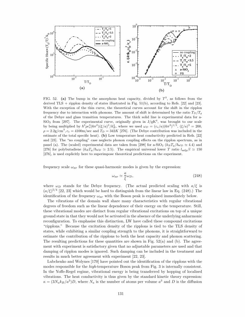
10-2

10-1

T/TD

104

105

106

Spec

ific

Hea

t (

TD

/T)3 /k

B

Tg/TD=5

Tg/TD=3.5

Tg/TD=2

no couplinga-SiO2

(a)

10-4

10-3

10-2

10-1

100

T/TD

10-4

10-3

10-2

10-1

100

κ/(

4πk B

ωD2

/cs)

no couplingTg/TD=2

Tg/TD=3.5

Tg/TD=5

a-SiO2PB

(b)

FIG. 52. (a) The bump in the amorphous heat capacity, divided by T 3, as follows from the

derived TLS + ripplon density of states illustrated in Fig. 51(b), according to Refs. [22] and [23].

With the exception of the thin curve, the theoretical curves account for the shift in the ripplon

frequency due to interaction with phonons. The amount of shift is determined by the ratio TD/Tg

of the Debye and glass transition temperatures. The thick solid line is experimental data for a-

SiO2 from [297]. The experimental curve, originally given in J/gK4, was brought to our scale

by being multiplied by ~3ρc3s(6π2)(ξ/a)3/k4B , where we used ωD = (cs/a)(6π2)1/3, (ξ/a)3 = 200,

ρ = 2.2g/cm3, cs = 4100m/sec and TD = 342K [276]. (The Debye contribution was included in the

estimate of the total specific heat). (b) Low temperature heat conductivity predicted in Refs. [22]

and [23]. The “no coupling” case neglects phonon coupling effects on the ripplon spectrum, as in

panel (a). The (scaled) experimental data are taken from [298] for a-SiO2 (kBTg/~ωD ≃ 4.4) and

[276] for polybutadiene (kBTg/~ωD ≃ 2.5). The empirical universal lower T ratio lmfp/l ≃ 150

[276], is used explicitly here to superimpose theoretical predictions on the experiment.

frequency scale ωBP for these quasi-harmonic modes is given by the expression:

ωBP ≃ a

ξωD, (248)

where ωD stands for the Debye frequency. (The actual predicted scaling with a/ξ is

(a/ξ)5/4 [22, 23] which would be hard to distinguish from the linear law in Eq. (248).) The

identification of the frequency ωBP with the Boson peak is explained immediately below.

The vibrations of the domain wall share many characteristics with regular vibrational

degrees of freedom such as the linear dependence of their energy on the temperature. Still,

these vibrational modes are distinct from regular vibrational excitations on top of a unique

ground state in that they would not be activated in the absence of the underlying anharmonic

reconfiguration. To emphasise this distinction, LW have called these compound excitations

“ripplons.” Because the excitation density of the ripplons is tied to the TLS density of

states, while exhibiting a similar coupling strength to the phonons, it is straightforward to

estimate the contribution of the ripplons to both the heat capacity and phonon scattering.

The resulting predictions for these quantities are shown in Fig. 52(a) and (b). The agree-

ment with experiment is satisfactory given that no adjustable parameters are used and that

damping of ripplon modes is ignored. Such damping can be included in the treatment and

results in much better agreement with experiment [22, 23].

Lubchenko and Wolynes [170] have pointed out the identification of the ripplons with the

modes responsible for the high-temperature Boson peak from Fig. 3 is internally consistent.

In the Yoffe-Regel regime, vibrational energy is being transferred by hopping of localised

vibrations. The heat conductivity is thus given by the standard kinetic theory expression:

κ = (3NakB/a3)D, where Na is the number of atoms per volume a3 and D is the diffusion

131

constant for hopping of localised vibrations. The length of the hop is determined by the

lattice spacing a, while the hop’s waiting time is determined by the vibrational lifetime, i.e.

τvibr. The resulting diffusion constant is D ≃ a2/6τvibr, so that the heat conductivity:

κ ≃ kBaτvibr

(Na/2). (249)

Using a = 3A, τvibr = 1 psec, and Na = 3 yields κ ≃ 0.1 W/m·K, in agreement with the typ-

ical experimental value of the conductivity near Tg [276]. In view of Eq. (249) and the slow

variation with temperature of the thermal conductivity above the Debye temperature,[276]

the vibrational relaxation time should indeed exhibit little temperature dependence well

below Tg. As a result, the corresponding peak in dielectric spectra should exhibit lit-

tle temperature dependence, as though a set of resonances intrinsic to the lattice were

responsible for the peak. Further, we recall Freeman and Anderson’s empirical observa-

tion [276] that κ’s for several different materials tend to saturate at a value numerically

close to (kBcs/a2)(4π)1/3(3Na)

2/3. Combining this observation with Eq. (249), we get

τ−1vibr ≃ (cs/a)2(4π/3Na)

1/3, i.e. a universal fraction of the Debye frequency. As temper-

ature is lowered, vibrational transfer should become less overdamped, but so should the

low-barrier tunnelling motions discussed above. We thus expect that the motions that give

rise to the high-T Boson peak will be mixed with the vibrations of the domain walls, when

both are present.

The relative unimportance of interaction between the structural resonances is a key fea-

ture of the present microscopic picture that distinguishes it from strong-interaction scenar-

ios [286–288]. The weakness of the interaction results from the low concentration of ther-

mally active resonances, as already mentioned. Still, each resonance is a multi-level system

with a rich structure. Transitions within an individual resonance are coupled to transitions

within the other resonances, via phonon exchange. This sort of off-diagonal coupling be-

tween local resonances lowers the energy [299] and is the mechanism of, for instance, the

dispersion interactions or the venerable Casimir effect. Lubchenko and Wolynes [23] (LW)

have pointed out that since the number of thermally active resonances in low temperature

glasses grows with temperature, so will the total amount of phonon-mediated attraction

between spatially separated portions of the sample. Depending on the amount of the local

anharmonicity of the lattice, this heating-induced attraction may thus result in a negative

thermal expansivity! Negative thermal expansivity is, in fact, observed in low temperature

glasses [300]. The magnitude of the “Casimir” effect in glasses depends sensitively on the

number of levels within an individual resonance. The results of LW analysis, which explicitly

included the ripplon states, are in quantitative agreement with observation thus providing

additional support for the RFOT-based microscopic picture of the resonances depicted in

Fig. 51(b).

As pointed out in the beginning of this Section, structural degeneracy is the key to the

presently discussed glassy anomalies, as opposed to effects of aperiodicity in a fully stable

lattice per se. We must be mindful that the vibrational response of stable aperiodic lattices

generally includes non-affine displacements [301], which also violate the Saint-Venant com-

patibility condition (110) [302]. These modes, which stem from a distribution in local elastic

response [303–305], have been proposed as the cause of the Boson Peak, requiring however

that the lattice be near its mechanical stability limit [21, 304, 306]. In the absence of such

marginal stability, purely elastic scattering seems too weak to account for the apparent

magnitude of phonon scattering at Boson Peak frequencies [23, 307, 308]. While the lack of

periodicity in glasses undoubtedly contributes to the excess phonon scattering, the presently

discussed structural resonances, which are inherently and strongly anharmonic processes,

account quantitatively for the apparent magnitude of the heat capacity and phonon scatter-

ing in a (logarithmically) broad temperature range that covers both the two-level system

132

and Boson peak dominated regimes. The reader is referred to the detailed discussion of the

combined distribution of the TLS parameters ǫ and ∆ from Eq. (242) by Lubchenko and

Wolynes [23]. In this treatment, the deviations of both the heat capacity and conductivity

from strict linear and quadratic temperature-dependences, respectively, are expected. While

the deviation is in the correct direction, its magnitude is somewhat below the observed value.

We note that only a relatively small number of regions host a zero-barrier mode at cryo-

genic temperatures: ξ3∫ T

0dǫ n(ǫ) ≃ T/Tg ≪ 1. This number, however, would be of the

order one near Tg thus seemingly implying that the glass would catastrophically liquefy

upon approaching the glass transition from below. This does not happen, of course. In

reality, the zero-barrier modes become increasingly dampened with increasing temperature.

This damping stems from the interaction of each individual bead movement along the tra-

jectory in Fig. 51(a) with the phonons. Quantitative estimation of this damping does not

appear to be straightforward. Empirically, however, the phonons are entirely dampened by

the high-T end of the plateau, and so should be elemental tunnelling motions, as the two

modes are completely hybridised by that point. Another way of saying that the individ-

ual bead motions are dampened to the fullest extent is that each bead is subject to the

regular viscous drag from the liquid. Under these circumstances, the calculation for the

reconfiguration rate from Section V applies.

B. The midgap electronic states

The cryogenic anomalies in glasses we have just discussed were a part of a thriving field

of research on amorphous materials in the 1970s. Much of this effort seems to have been

driven by potential applications in renewable energy. For instance, amorphous silicon was

regarded to be a promising candidate material for photovoltaic applications. Another family

of amorphous semiconductors was also studied, namely, the so called chalcogenide alloys,

which contain “chalcogens,” i.e., elements from group XVI (S, Se, Te) and, often, “pnicto-

gens,” i.e., elements from group XV (P, As, Sb, Bi) and also elements from group XIV (Si,

Ge). Archetypal representatives of this group of compounds are As2S3 and As2Se3; both

are good glassformers. More recently, chalcogenides have gained prominence in the con-

text of applications in opto-electronics [3–9] and are often called “phase-change materials,”

since their optical and electric properties can be readily “switched” [309] by converting the

material between its crystalline and amorphous form.

The chalcogenides were first brought into prominence by the Kolomiets lab, including

their remarkable property of being insensitive to doping [272, 310]. This is in contrast with

traditional semiconductors, whose conductance can be manipulated by adding elements that

prefer to bond to fewer or more atoms than the host species. Note that the prevailing view

of amorphous insulators seems that they are not too different from their crystalline coun-

terparts. Within the Anderson localisation paradigm [271, 311], these aperiodic materials

can still convey electricity within continuous mobility bands made of overlapping orbitals.

In addition, there are exponential (Urbach) tails of localised states extending away from

the mobility bands, which may serve as efficient traps for charge carriers [273, 274]. Since

the tails decay exponentially quickly, one may still speak of relatively well-defined mobility

gaps.

While the ability of an equilibrated amorphous lattice to accommodate a broad range of

bonding preferences of individual atoms is perhaps not too surprising, the apparent strict

pinning of the Fermi level in amorphous chalcogenides does beg for explanation. What is

even more puzzling, these materials cannot be doped extraneously yet, at the same time,

they seem to possess a robust, intrinsic number of defect-like, midgap states. The latter

states become apparent upon irradiation of an amorphous chalcogenide with high intensity

133

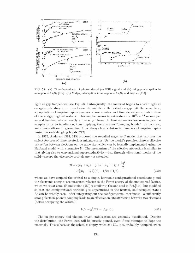
(a)(b)

FIG. 53. (a) Time-dependence of photoinduced (a) ESR signal and (b) midgap absorption in

amorphous As2S3 [312]. (b) Midgap absorption in amorphous As2S3 and As2Se3 [313].

light at gap frequencies, see Fig. 53. Subsequently, the material begins to absorb light at

energies extending to or even below the middle of the forbidden gap. At the same time,

a population of unpaired spins emerges whose number and time dependence match those

of the midgap light-absorbers. This number seems to saturate at ∼ 1020cm−3 or one per

several hundred atoms, nearly universally. None of these anomalies are seen in pristine

samples prior to irradiation, thus implying there are no “dangling bonds.” In contrast,

amorphous silicon or germanium films always host substantial numbers of unpaired spins

hosted on such dangling bonds [272].

In 1975, Anderson [314, 315] proposed the so-called negative-U model that captures the

salient features of these mysterious midgap states. By the model’s premise, there is effective

attraction between electrons on the same site, which can be formally implemented using the

Hubbard model with a negative U . The mechanism of the effective attraction is similar to

that giving rise to conventional superconductivity—i.e., through vibrational modes of the

solid—except the electronic orbitals are not extended:

H = ǫ(n↑ + n↓)− g(n↑ + n↓ − 1)q +kq2

2+ U [(n↑ − 1/2)(n↓ − 1/2) + 1/4], (250)

where we have coupled the orbital to a single, harmonic configurational coordinate q and

the electronic energies are measured relative to the Fermi energy of the undistorted lattice,

which we set at zero. (Hamiltonian (250) is similar to the one used in Ref.[314], but modified

so that the configurational variable q is unperturbed in the neutral, half-occupied state.)

As can be readily seen—after integrating out the configurational coordinate—a sufficiently

strong electron-phonon coupling leads to an effective on-site attraction between two electrons

(holes) occupying the orbital:

U/2− g2/2k = Ueff < 0. (251)

The on-site energy and phonon-driven stabilisation are generally distributed. Despite

the distribution, the Fermi level will be strictly pinned, even if one attempts to dope the

materials. This is because the orbital is empty, when 2ǫ+Ueff > 0, or doubly occupied, when

134

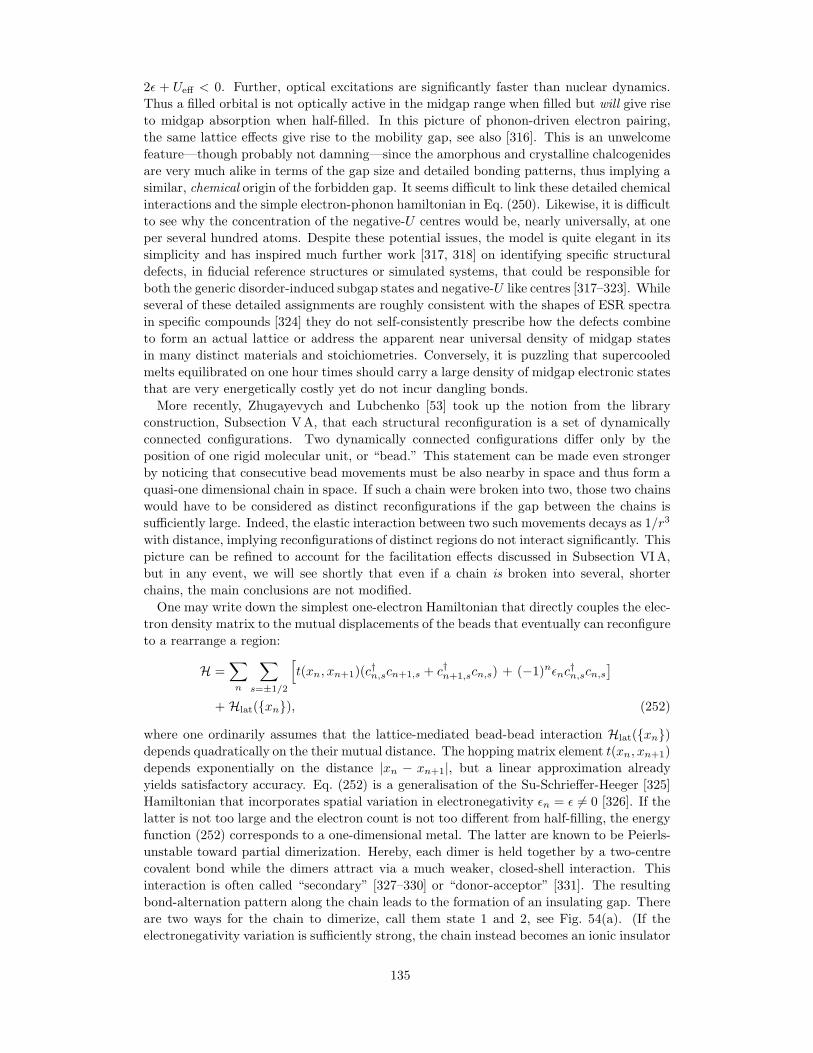
2ǫ + Ueff < 0. Further, optical excitations are significantly faster than nuclear dynamics.

Thus a filled orbital is not optically active in the midgap range when filled but will give rise

to midgap absorption when half-filled. In this picture of phonon-driven electron pairing,

the same lattice effects give rise to the mobility gap, see also [316]. This is an unwelcome

feature—though probably not damning—since the amorphous and crystalline chalcogenides

are very much alike in terms of the gap size and detailed bonding patterns, thus implying a

similar, chemical origin of the forbidden gap. It seems difficult to link these detailed chemical

interactions and the simple electron-phonon hamiltonian in Eq. (250). Likewise, it is difficult

to see why the concentration of the negative-U centres would be, nearly universally, at one

per several hundred atoms. Despite these potential issues, the model is quite elegant in its

simplicity and has inspired much further work [317, 318] on identifying specific structural

defects, in fiducial reference structures or simulated systems, that could be responsible for

both the generic disorder-induced subgap states and negative-U like centres [317–323]. While

several of these detailed assignments are roughly consistent with the shapes of ESR spectra

in specific compounds [324] they do not self-consistently prescribe how the defects combine

to form an actual lattice or address the apparent near universal density of midgap states

in many distinct materials and stoichiometries. Conversely, it is puzzling that supercooled

melts equilibrated on one hour times should carry a large density of midgap electronic states

that are very energetically costly yet do not incur dangling bonds.

More recently, Zhugayevych and Lubchenko [53] took up the notion from the library

construction, Subsection VA, that each structural reconfiguration is a set of dynamically

connected configurations. Two dynamically connected configurations differ only by the

position of one rigid molecular unit, or “bead.” This statement can be made even stronger

by noticing that consecutive bead movements must be also nearby in space and thus form a

quasi-one dimensional chain in space. If such a chain were broken into two, those two chains

would have to be considered as distinct reconfigurations if the gap between the chains is

sufficiently large. Indeed, the elastic interaction between two such movements decays as 1/r3

with distance, implying reconfigurations of distinct regions do not interact significantly. This

picture can be refined to account for the facilitation effects discussed in Subsection VIA,

but in any event, we will see shortly that even if a chain is broken into several, shorter

chains, the main conclusions are not modified.

One may write down the simplest one-electron Hamiltonian that directly couples the elec-

tron density matrix to the mutual displacements of the beads that eventually can reconfigure

to a rearrange a region:

H =∑

n

∑

s=±1/2

[t(xn, xn+1)(c

†n,scn+1,s + c†n+1,scn,s) + (−1)nǫnc

†n,scn,s

]

+ Hlat(xn), (252)

where one ordinarily assumes that the lattice-mediated bead-bead interaction Hlat(xn)depends quadratically on the their mutual distance. The hopping matrix element t(xn, xn+1)

depends exponentially on the distance |xn − xn+1|, but a linear approximation already

yields satisfactory accuracy. Eq. (252) is a generalisation of the Su-Schrieffer-Heeger [325]

Hamiltonian that incorporates spatial variation in electronegativity ǫn = ǫ 6= 0 [326]. If the

latter is not too large and the electron count is not too different from half-filling, the energy

function (252) corresponds to a one-dimensional metal. The latter are known to be Peierls-

unstable toward partial dimerization. Hereby, each dimer is held together by a two-centre

covalent bond while the dimers attract via a much weaker, closed-shell interaction. This

interaction is often called “secondary” [327–330] or “donor-acceptor” [331]. The resulting

bond-alternation pattern along the chain leads to the formation of an insulating gap. There

are two ways for the chain to dimerize, call them state 1 and 2, see Fig. 54(a). (If the

electronegativity variation is sufficiently strong, the chain instead becomes an ionic insulator

135

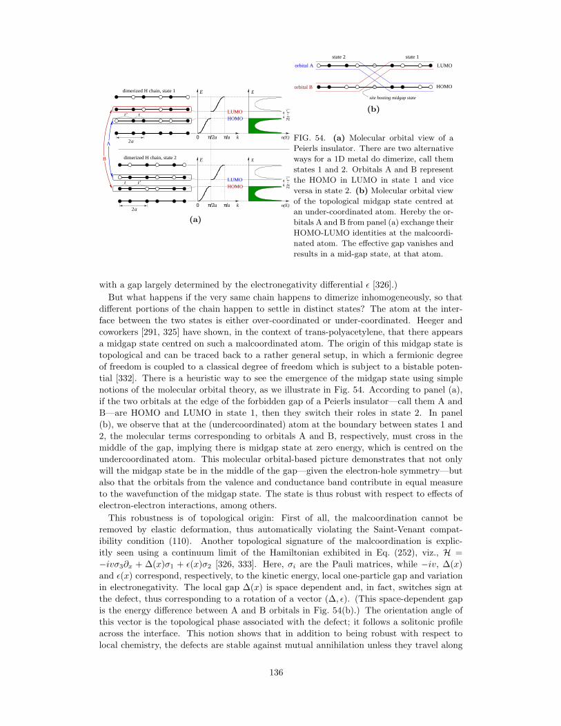
π/a

2a

t−t’

2|

|

t t’

t’ t

2a

a n(E)

E

k0

E

π/2a

n(E)

E

k0

E

π/2a

dimerized H chain, state 1

dimerized H chain, state 2

LUMO

LUMO

π/

t−t’

2|

|

HOMO

HOMO

A

B

(a)

LUMO

site hosting midgap state

state 1state 2

orbital A

orbital B HOMO

(b)

FIG. 54. (a) Molecular orbital view of a

Peierls insulator. There are two alternative

ways for a 1D metal do dimerize, call them

states 1 and 2. Orbitals A and B represent

the HOMO in LUMO in state 1 and vice

versa in state 2. (b) Molecular orbital view

of the topological midgap state centred at

an under-coordinated atom. Hereby the or-

bitals A and B from panel (a) exchange their

HOMO-LUMO identities at the malcoordi-

nated atom. The effective gap vanishes and

results in a mid-gap state, at that atom.

with a gap largely determined by the electronegativity differential ǫ [326].)

But what happens if the very same chain happens to dimerize inhomogeneously, so that

different portions of the chain happen to settle in distinct states? The atom at the inter-

face between the two states is either over-coordinated or under-coordinated. Heeger and

coworkers [291, 325] have shown, in the context of trans-polyacetylene, that there appears

a midgap state centred on such a malcoordinated atom. The origin of this midgap state is

topological and can be traced back to a rather general setup, in which a fermionic degree

of freedom is coupled to a classical degree of freedom which is subject to a bistable poten-

tial [332]. There is a heuristic way to see the emergence of the midgap state using simple

notions of the molecular orbital theory, as we illustrate in Fig. 54. According to panel (a),

if the two orbitals at the edge of the forbidden gap of a Peierls insulator—call them A and

B—are HOMO and LUMO in state 1, then they switch their roles in state 2. In panel

(b), we observe that at the (undercoordinated) atom at the boundary between states 1 and

2, the molecular terms corresponding to orbitals A and B, respectively, must cross in the

middle of the gap, implying there is midgap state at zero energy, which is centred on the

undercoordinated atom. This molecular orbital-based picture demonstrates that not only

will the midgap state be in the middle of the gap—given the electron-hole symmetry—but

also that the orbitals from the valence and conductance band contribute in equal measure

to the wavefunction of the midgap state. The state is thus robust with respect to effects of

electron-electron interactions, among others.

This robustness is of topological origin: First of all, the malcoordination cannot be

removed by elastic deformation, thus automatically violating the Saint-Venant compat-

ibility condition (110). Another topological signature of the malcoordination is explic-

itly seen using a continuum limit of the Hamiltonian exhibited in Eq. (252), viz., H =

−ivσ3∂x + ∆(x)σ1 + ǫ(x)σ2 [326, 333]. Here, σi are the Pauli matrices, while −iv, ∆(x)

and ǫ(x) correspond, respectively, to the kinetic energy, local one-particle gap and variation

in electronegativity. The local gap ∆(x) is space dependent and, in fact, switches sign at

the defect, thus corresponding to a rotation of a vector (∆, ǫ). (This space-dependent gap

is the energy difference between A and B orbitals in Fig. 54(b).) The orientation angle of

this vector is the topological phase associated with the defect; it follows a solitonic profile

across the interface. This notion shows that in addition to being robust with respect to

local chemistry, the defects are stable against mutual annihilation unless they travel along

136

exactly the same chain. Indeed, the phases of defects travelling along different paths can

not cancel.

The midgap states are remarkable in several ways: First of all, they exhibit a charge-spin

relation opposite from that expected for a regular fermion: A neutral defect is half-filled

and thus has spin 1/2; a charged state is paramagnetic. From a chemist’s viewpoint, a

neutral defect is merely a free radical solvated in a solid matrix. Last but not least, the

wave-function of the midgap state is surprisingly extended. Indeed, a simple estimate shows

that a generic bound state at ∼ 1eV below a continuum should be of atomic dimensions. In

contrast, both the wavefunction and the solitonic deformation pattern of the 1D lattice are

about 10 lattice spacings across, for a semiconducting material [53]. (In trans-polyacetylene,

this extent is as large as 20 lattice spacings because of the low effective mass of the electron in

this material.) Thus, the malcoordination is evenly distributed over a considerable distance.

Note that the bond length at the centre of the malcoordination is about midway between

that of the long and short bond, also implying an intermediate bond strength.

In the ZL scenario, the effective attraction between two electrons/holes occupying the

midgap state, if any, is not directly tied to the magnitude of the gap. Instead, it is a

relatively subtle effect that stems from the attraction between a charge and a neutral radical

embedded in a dielectric medium. While one expects such an attraction when the radical-

plus-matrix system is sufficiently polarisable, its presence is not a given. We will return

to this point shortly. In the most significant contrast with Anderson’s phenomenological

negative-U model and the subsequent ultralocal defect views [317–323], the midgap states

intrinsically stem from the structural degeneracy of the lattice and are topologically stable.

The concentration of the midgap states is determined by the concentration of the domain

walls near the glass transition, an equilibrium quantity:

nDW(Tg) ≃ 1/ξ(Tg)3 ≃ 1020cm−3, (253)

consistent with observation. For the ZL [53] scenario to work, at least two basic requirements

must be fulfilled by the material: (a) the bonds along the chain should not be saturated,

and (b) the insulating gap should not be too large, since in this case the chain is an ionic

insulator, as opposed to a Peierls insulator. Only one family of known glassformers seems

to satisfy these restrictions, namely, the chalcogenides. Already this can be used to argue

circumstantially for the presence of the midgap states in these materials.

It turns out that in the specific case of chalcogenide glasses, the specific atomic motifs lead-

ing to the midgap states can be directly identified based on a relatively simple chemical yet

constructive picture. As the first step in their argument, Zhugayevych and Lubchenko [29]

(ZL) argue that these materials are symmetry broken and distorted versions of much sim-

pler, “parent” structures defined on the simple cubic lattice. This idea builds on the work

of Burdett and coworkers on the structure of solid arsenic and electronically similar com-

pounds [334, 335]. Similarly, the crystal of As2Se3 can be thought of as a distorted version

of the parent structure in Fig. 55(a), in which some of the vertices are occupied by vacancies.

Each link in the parent structure corresponds with a covalent bond in the actual, distorted

structure, whereas a gap will give rise to a secondary bond. The actual, distorted struc-

ture is much more complicated that its parent, see Fig. 55(b). The cause of the symmetry

breaking in these 3D structures can no longer be traced with confidence to the Peierls insta-

bility, especially in view of the significant sp-mixing in these compounds [336], see, however,

Ref. [337]. Still, the very fact of symmetry breaking between two adjacent covalent and

secondary bonds that are nearly co-linear is documented on thousands of compounds [329].

Much as the crystal of As2Se3 can be thought of as a distorted version of the parent

structure in Fig. 55(a), chalcogenide glasses can also be thought of as being distorted versions

of parent structures in which atoms and vacancies are placed aperiodically. In either case,

a pnictogen (chalcogen) forms three (two) covalent bonds with its nearest neighbours and

137

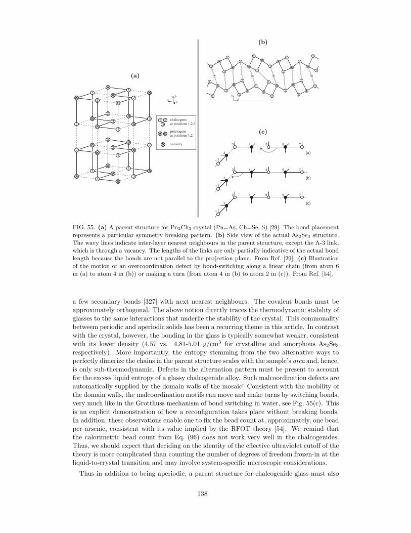
(a)

11

3

3

22

2

AA

A

B3

BB

BB

AA

1

2

33

3

1

B

A

22

11

a

bc

pnictogensat positions 1,2

1 23

A B

chalcogensat positions 1,2,3

vacancy

(b)

bc

bc

bc

bc

bc bc

bcbcbc

bc

bc

bc

bcbc

bc

bc

bcbc

bC

bC

bC

bC

bC

bC

bC

bC

bC

bC

bC

bC

bC

bC

bC

bCbC

bC

bCbC

bC

bC

bCbC

bc bc bc bc× × × ×

A

A

A

A

A A

A

A

B

B

B

B

B

B

1

1

1

1

1

1

1

1

2

2

2

2

2

2

2

2

3

3

3

3

3

3

33

a

b

(c)

54 6 73

1

2

54 6 73

1

2

54 6 73

1

2 (a)

(b)

(c)

FIG. 55. (a) A parent structure for Pn2Ch3 crystal (Pn=As, Ch=Se, S) [29]. The bond placement

represents a particular symmetry breaking pattern. (b) Side view of the actual As2Se3 structure.

The wavy lines indicate inter-layer nearest neighbours in the parent structure, except the A-3 link,

which is through a vacancy. The lengths of the links are only partially indicative of the actual bond

length because the bonds are not parallel to the projection plane. From Ref. [29]. (c) Illustration

of the motion of an overcoordination defect by bond-switching along a linear chain (from atom 6

in (a) to atom 4 in (b)) or making a turn (from atom 4 in (b) to atom 2 in (c)). From Ref. [54].

a few secondary bonds [327] with next nearest neighbours. The covalent bonds must be

approximately orthogonal. The above notion directly traces the thermodynamic stability of

glasses to the same interactions that underlie the stability of the crystal. This commonality

betweem periodic and aperiodic solids has been a recurring theme in this article. In contrast

with the crystal, however, the bonding in the glass is typically somewhat weaker, consistent

with its lower density (4.57 vs. 4.81-5.01 g/cm3 for crystalline and amorphous As2Se3respectively). More importantly, the entropy stemming from the two alternative ways to

perfectly dimerize the chains in the parent structure scales with the sample’s area and, hence,

is only sub-thermodynamic. Defects in the alternation pattern must be present to account

for the excess liquid entropy of a glassy chalcogenide alloy. Such malcoordination defects are

automatically supplied by the domain walls of the mosaic! Consistent with the mobility of

the domain walls, the malcoordination motifs can move and make turns by switching bonds,

very much like in the Grotthuss mechanism of bond switching in water, see Fig. 55(c). This

is an explicit demonstration of how a reconfiguration takes place without breaking bonds.

In addition, these observations enable one to fix the bead count at, approximately, one bead

per arsenic, consistent with its value implied by the RFOT theory [54]. We remind that

the calorimetric bead count from Eq. (96) does not work very well in the chalcogenides.

Thus, we should expect that deciding on the identity of the effective ultraviolet cutoff of the

theory is more complicated than counting the number of degrees of freedom frozen-in at the

liquid-to-crystal transition and may involve system-specific microscopic considerations.

Thus in addition to being aperiodic, a parent structure for chalcogenide glass must also

138

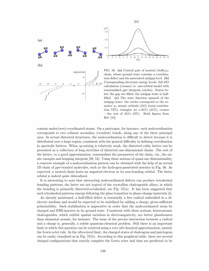
(a)

(b)

2−2−4−6−8−10−12

−10

10

E, eV

eigenstate

bCbCbC

bCbC

bCbC

bCbCbC

bCbCbCbCbCbCbCbCbCbCbC

XXXXXXXXXXXXXX

XX

XX

XXX

XXXXXXXXXXX

XXXXXXXXXXX

bCX

(c)

3 4 5 6 7 8 9 10 11 12 13 14 15 16 17 18 190

0.1

0.2

0.3

site

|ψ|2

bC bC

bC

bC

bC

bC

bC

bC bCuT uTuT

uT uT

uTuT uTX X X

X XX X X

FIG. 56. (a) Central part of neutral (AsH2)21chain, whose ground state contains a coordina-

tion defect and the associated midgap level. (b)

Corresponding electronic energy levels: full MO

calculation (crosses) vs. one-orbital model with

renormalised ppσ integrals (circles). States be-

low the gap are filled; the midgap state is half-

filled. (c) The wave function squared of the

midgap state: the circles correspond to the ar-

senics’ pz atomic orbitals (AO) (total contribu-

tion 73%), triangles As s-AO’s (21%), crosses

– the rest of AO’s (6%). Both figures from

Ref. [54].

contain under(over)-coordinated atoms. On a pnictogen, for instance, such malcoordination

corresponds to two colinear secondary (covalent) bonds, along any of the three principal

axes. In actual distorted structures, the malcoordination is difficult to detect because it is

distributed over a large region, consistent with the general difficulty in defining coordination

in aperiodic lattices. When sp-mixing is relatively weak, the distorted cubic lattice can be

presented as a collection of long stretches of distorted one-dimensional chains. The rest of

the lattice, to a good approximation, renormalises the parameters of the chain, viz., the on-

site energies and hopping integrals [29, 54]. Using these notions of quasi-one dimensionality,

a concrete example of a malcoordination pattern can be obtained with the help of an actual

1D chain of ppσ-bonded molecules, such as the hydrogen-passivated arsenics in Fig. 56. As

expected, a neutral chain hosts an unpaired electron in its non-bonding orbital. The latter

orbital is indeed quite delocalized.

It is interesting to note that interacting malcoordinated defects can produce tetrahedral

bonding patterns; the latter are not typical of the crystalline chalcogenide alloys, in which

the bonding is primarily distorted-octahedral, see Fig. 57(a). It has been suggested that

such tetrahedral patterns emerge following the glass transition in phase-change materials [4].

As already mentioned, a half-filled defect is essentially a free radical embedded in a di-

electric medium and would be expected to be stabilised by adding a charge, given sufficient

polarisability. Such stabilisation is imperative in order that the malcoordinated atom be

charged and ESR-inactive in its ground state. Consistent with these notions, heteroatomic

chalcogenides, which exhibit spatial variation in electronegativity, are better glassformers

than elemental arsenic, for instance. The issue of the precise interaction between a radical

and a charge is, generally, a subtle quantum-chemical problem. Still there is an important

limit in which this question can be resolved using a very old chemical approximation, namely

the Lewis octet rule. In the ultra-local limit, the charged states of chalcogens and pnictogens

can be easily visualised as in Fig. 57(b). According to this graphical table, there are several

charged configurations that exactly complete the Lewis octet and thus are predicted to be

139

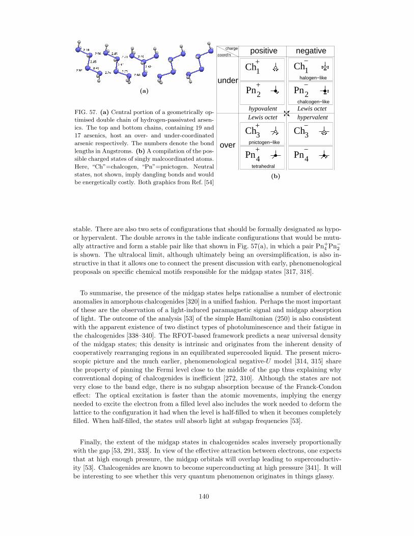
(a)

FIG. 57. (a) Central portion of a geometrically op-

timised double chain of hydrogen-passivated arsen-

ics. The top and bottom chains, containing 19 and

17 arsenics, host an over- and under-coordinated

arsenic respectively. The numbers denote the bond

lengths in Angstroms. (b) A compilation of the pos-

sible charged states of singly malcoordinated atoms.

Here, “Ch”=chalcogen, “Pn”=pnictogen. Neutral

states, not shown, imply dangling bonds and would

be energetically costly. Both graphics from Ref. [54]

coord’n

2+

Ch1+ Ch1

−

Pn2−

Pn+4

chalcogen−like

tetrahedral

halogen−like

Lewis octetLewis octethypovalent

under

over

charge

Pn

Ch+3

positive negative

Ch−3

Pn−4

hypervalent

pnictogen−like

(b)

stable. There are also two sets of configurations that should be formally designated as hypo-

or hypervalent. The double arrows in the table indicate configurations that would be mutu-

ally attractive and form a stable pair like that shown in Fig. 57(a), in which a pair Pn+4 Pn−2

is shown. The ultralocal limit, although ultimately being an oversimplification, is also in-

structive in that it allows one to connect the present discussion with early, phenomenological

proposals on specific chemical motifs responsible for the midgap states [317, 318].

To summarise, the presence of the midgap states helps rationalise a number of electronic

anomalies in amorphous chalcogenides [320] in a unified fashion. Perhaps the most important

of these are the observation of a light-induced paramagnetic signal and midgap absorption

of light. The outcome of the analysis [53] of the simple Hamiltonian (250) is also consistent

with the apparent existence of two distinct types of photoluminescence and their fatigue in

the chalcogenides [338–340]. The RFOT-based framework predicts a near universal density

of the midgap states; this density is intrinsic and originates from the inherent density of

cooperatively rearranging regions in an equilibrated supercooled liquid. The present micro-

scopic picture and the much earlier, phenomenological negative-U model [314, 315] share

the property of pinning the Fermi level close to the middle of the gap thus explaining why

conventional doping of chalcogenides is inefficient [272, 310]. Although the states are not

very close to the band edge, there is no subgap absorption because of the Franck-Condon

effect: The optical excitation is faster than the atomic movements, implying the energy

needed to excite the electron from a filled level also includes the work needed to deform the

lattice to the configuration it had when the level is half-filled to when it becomes completely

filled. When half-filled, the states will absorb light at subgap frequencies [53].

Finally, the extent of the midgap states in chalcogenides scales inversely proportionally

with the gap [53, 291, 333]. In view of the effective attraction between electrons, one expects

that at high enough pressure, the midgap orbitals will overlap leading to superconductiv-

ity [53]. Chalcogenides are known to become superconducting at high pressure [341]. It will

be interesting to see whether this very quantum phenomenon originates in things glassy.

140

XIII. SUMMARY AND CONNECTION WITH JAMMED AND OTHER TYPES

OF APERIODIC SOLIDS

In an informal remark dating from 1995, P. W. Anderson writes [342]: “The deepest

and most interesting unsolved problem in solid state theory is probably the theory of the

glass and the glass transition. This could be the next breakthrough in the coming decade.”

It is probably fair to say that the problem of the structural glass transition has been as

interesting and challenging as it has been controversial. So much so that it found a way into

mass media some thirteen years after Anderson’s remark was published [343].

The reader has undoubtedly noticed that the present author feels significantly more secure

about the current status of the theory of the glass transition than what the readers of the

New York Times might infer from several less-than-optimistic views expressed in Ref. [343].

Although the RFOT theory uses approximations, the physical picture of the structural glass

transition presented bu it is constructive and quantitative. It uses well-established concepts

of the classical density functional theory (DFT) complemented by more recent insight about

systems with relatively complicated free energy landscapes; hereby the distinct free energy

minima correspond to long-lived, but not infinitely-lived states. Although it is often difficult

to treat finite-lifetime states using methods developed in equilibrium thermodynamics, such

methods become quantitative (and physically transparent) given sufficient time scale sep-

aration between motions of individual particles and the progress coordinate that describes

the escape from the long-lived states. Many examples of successful quantitative descriptions

of such long-lived states exist, such as the transition state theory [199, 200, 296, 344], and,

in particular, as applied to nucleation phenomena. The RFOT description takes advantage

of the accuracy of the transition state theory to determine the distribution of the relaxation

rates and cooperativity sizes in glassy liquids, without using adjustable parameters; in turn

this allows one to predict the glass transition temperature (on a given timescale) using ex-

perimentally determined values of a specific quantity, viz., the excess liquid entropy. This

quantity is defined and measured without reference to the glass transition itself. It should

not be held against the theory that it cannot (yet) predict the configurational entropy for

actual compounds, but only for model substances. Much the same way, we do not hold

against existing theories of liquid-to-crystal transition that they cannot determine the melt-

ing point for actual compounds, but only can predict melting points for model substances

with known interactions.

We have seen that the complicated free energy landscape of a glassy liquid begins to form

when a uniform liquid undergoes a breaking of the translational symmetry, upon which the

equilibrium density profile is no longer flat but consists of disparate, narrow peaks; the

locations of the peaks form an aperiodic lattice. The breaking of the symmetry is driven by

steric effects, as can be shown using independent arguments from the classical density func-

tional theory, the mode-coupling theory, and a symmetry-breaking perspective afforded by

the Landau-Ginzburg expansion. The density-driven symmetry breaking is entirely analo-

gous to that during a density driven transition from the uniform liquid to a periodic crystal,

although somewhat less so when the crystal structure is very open and mostly determined

by directional bonding. In contrast with the periodic crystallisation, the peaks in the ape-

riodic structure are not entirely stationary but move about in an intermittent, cooperative

fashion; if watched for a sufficiently long time, the liquid density profile becomes uniform

again. These motions correspond to transitions between distinct metastable free energy

minima and, hence, are driven by the complexity of the free energy landscape. For this spe-

cial mechanism to work, the number of free energy minima must scale exponentially with

the region size; the log-number per particle is called the configurational entropy sc > 0.

This vast structural degeneracy introduces new physics in the problem, along with new

length and time scales. It is entropically unfavourable for a glassy system to reside in

141

any given free energy minimum forever. The system thus undergoes local transitions to

alternative metastable states. In the mean-field limit, it is possible to think of the liquid

as a mosaic of regions, each of which is occupied by a structure corresponding to one of

the mean-field free energy minima. The interfaces between the mosaic cells are made up of

configurations corresponding to the barrier in the bulk free energy separating the minima.

In finite dimensions, the picture is no longer as simple, but the liquid can still be thought

of as a mosaic of regions characterised by relatively low free energy density separated by

regions at relatively high free energy density. Each stable region can be thought of as being

trapped in a state produced by negative free energy fluctuations, from a relatively high

free energy state typical of the liquid that just begins to enter the landscape regime. Not

every negative fluctuation would be long-lived, however, but only such that also happens

to coincide with a transition to a specific free energy minimum. This is something that

would be impossible in a landscape-free system that has a sub-thermodynamic number of

alternative minima. Matching the magnitude of the stabilisation due to the fluctuation with

the entropic stabilisation due to the complexity of the landscape, δG = TscN , yields the

size N∗ of the region that was stabilised by the fluctuation. This size is finite because the

fluctuation size scales sublinearly with N : δG = γ√N . (Note the equation γ

√N = TscN

has no finite solutions when sc is strictly zero.) Conversely, N∗ is the region size that

must be reconfigured (in equilibrium) for the liquid to escape the free energy minimum it is

currently trapped in. It is the latter perspective that is worked out in the microscopic picture

presented here. It is shown that the escape from the current minimum can be thought of

as an activated, nucleation-like event driven by the multiplicity of the free energy minima,

−TscN , but is subject to a mismatch penalty between the initial and final states. If one

takes the stabilised state as the free energy reference, the mismatch penalty to flip a region

of size N is the typical magnitude of the free energy fluctuation: γ√N , Eq. (153). The

resulting escape barrier is simply F ‡ = γ2/4scT . This formalism yields many quantitative

predictions, including, in particular, the α-relaxation barrier and the cooperativity length

and those predictions can directly be extended to non-equilibrium situations, such as ageing.

A great deal of these predictions have to do with the local fluctuations in the structural

degeneracy, which are directly reflected in the heat capacity jump at the glass transition.

Hereby the intrinsic connections are revealed between the deviations from the Arrhenius

temperature dependence of α-relaxation, relaxations’ exponentiality, and the fluctuation

dissipation theorem.

Although transitions to both periodic and aperiodic crystal are discontinuous—the restor-

ing force in response to finite wavelength deformation becomes finite via a discrete jump—the

onset of measured rigidity in glassy liquid is gradual. This is because the spatial extent and

lifetime of the long-lived structures increase continuously with lowering temperature and/or

increasing pressure. The material becomes macroscopically rigid, if quenched sufficiently

below the glass transition temperature Tg. This is because the the barrier for activated

transitions, which is about 35 . . .39kBTg, becomes very large compared with the ambient

temperature, not because the structure represents a unique energy minimum. (In fact,

glasses are vastly structurally degenerate, in contradistinction with periodic crystals.) In

this way, the rigidity of glasses and periodic crystals are subtly different. Still, relics of

the structural reconfigurations that give rise to liquid flow above the glass transition survive

down to very low, sub-Kelvin temperatures. These relics can be counted and turn out to fully

account for the mysterious structural resonances people have phenomenologically associated

with the so called two-level systems. The physical boundaries of the reconfigurations—or

domain walls—are interesting objects in themselves: On the one hand, their vibrations

quantitatively account for the famous Boson peak. (These vibrations can be thought of as

the Goldstone modes that emerge when the mosaic forms.) On the other hand, the domain

walls can host very special electronic states under certain circumstances that are physically

142

realised in amorphous chalcogenide alloys. The latter alloys have come back into prominence

owing to their potential as phase-change memory materials.

As just said, the emergence of the landscape is the result of a discontinuous transition

and, in fact, could be thought of an avoided critical point, see Fig. 7. In the absence of

strongly-directional bonding, the criticality is avoided in equilibrium owing to steric effects,

which stabilise locally dense structures. This can be seen using already a Landau-Ginzburg

expansion and, quantitatively, the classical DFT. A quantitative criterion of the proximity

to the critical point is the ratio of the volumetric particle size a and the magnitude dLof the vibrational displacement near the mechanical stability limit of the aperiodic solid.

In the case of aperiodic solids it is exactly the inverse of the venerable Lindemann ratio.

By Eq. (83), the (a/dL) ratio scales linearly with the dimensionality of space, up to a

logarithmic correction and factor of order 1. In 3D, both experiment and calculation yield,

nearly universally, (a/dL) ≃ 101 for a solid in equilibrium with the corresponding uniform

liquid, be the solid periodic or aperiodic. For the liquid-to-solid transition to be continuous,

this ratio would have to be close to 100. The (a/dL) ratio reappears under several guises

during the analysis, because its square corresponds with the elastic modulus of the substance

in terms of kBT , by equipartition: (a/dL)2 ≃ Ka3/kBT . (K is the bulk modulus.) We have

seen that this ratio corresponds with the excess relaxation time in a liquid compared to

the corresponding solid. This mismatch is behind the kinetic catastrophe of the mode-

coupling theory. The (a/dL)2 ratio also enters in the expression for the escape barrier F ‡

since, approximately, δG2/N ≡ γ2 ∝ K. Appropriately, the activated reconfigurations do

not involve breaking of individual bonds; in fact dL ≃ a/10 is comparable to the typical

vibrational magnitude. Despite the near harmonic nature of the motions of individual

atoms, the overall reconfiguration event is strongly anharmonic, see Fig. 25(a). Specific

microscopic realisations of such chemically-mild local motions have been identified. For

instance, a covalent bond in glassy chalcogenides can gradually weaken into a secondary

and, then, a van der Waals bond, before finally rupturing [29, 54]. This is quite similar

to the Grotthuss mechanism of bond switching in water. Another often-cited example is

the rotations of the SiO4/2 tetrahedra in glassy silica, during which covalent bonds are not

broken but only distorted following a reconfiguration event. Yet another way to look at this

chemically-interesting aspect of the landscape regime is provided by very very old samples of

amber, which exhibit the cryogenic two-level systems and Boson peak despite the significant

amount of cross-linking that took place over 108 years ago [345].

The (dL/a) ratio may thus be legitimately thought of as the small parameter of the

theory, non-withstanding the subtlety associated with the fact that this small parameter is

not fixed upfront but is self-generated as a result of a discontinuous transition. Consistent

with the lack of critical-like fluctuations, the correlation length for fluctuations in glassy

liquids, has been shown to be comparable to the molecular length scale [32]. As a result,

the cooperativity can be argued to be somewhat trivial, viz., due to ordinary Gaussian

fluctuations. (A case for sub-dominant fluctuations stemming from wandering of the domain

walls has been made recently [209].)

In contrast with substances in the landscape regime, amorphous films made of a poor

glass-former that favours open structures, such as silicon or water at normal pressure, would

rearrange by bond-breaking. Accordingly, energy quantities reflecting bond strength—as

opposed to bond elasticity—would determine the barrier. (Note bond strength and elasticity

are correlated in actual materials [105], because the atomic size varies relatively little across

the periodic table and so the depth of a bounding potential must correlate with its curvature

at the bottom.) Materials with open structures largely avoid entering the landscape regime

because of the relative unimportance of the steric effects and thus are “unaware” of the

aforementioned criticality in the first place. The bond directionality could be so strong that

the liquid could expand upon freezing. Even in supercooled silicon, coordination decreases

143

with cooling [346]. Amorphous films made of such directionally bonding particles are even

more open than the crystal and exhibit dangling bonds. In such films, which can be made

by rapid quench or by sputtering on a cold substrate, steric effects are even less important

than in corresponding crystals. In a way, one can think of such amorphous films as very

cross-linked gels or vulcanised rubbers. Although generally aperiodic, these materials may

be in the landscape regime only to a marginal extennt. The steric interactions set the nearest

neighbour distance but not the coordination pattern itself; as a result the films reconfigure

predominantly by bond breaking. These notions are consistent with the apparent scarcity of

cryogenic excitations in silicon and germanium films [210, 293, 294]. The latter excitations

are predicted to be intrinsic (and quantum!) features of landscape systems. To summarise,

materials that favour open structures avoid the landscape regime by either crystallising

or forming gel-like aperiodic structures. While such aperiodic open structures may share

some properties with glasses made by quenching an equilibrated liquid, these properties

are expected to be quite system-specific, in contrast with glasses, whose key microscopic

properties are set by the cooperativity length at the glass transition and the glass transition

temperature itself.

To avoid confusion we note that materials with very directional bonding may be poor

glassformers at ordinary pressures but could be vitrified more readily following pressurisa-

tion [138–141], which would make steric repulsion more prominent. This is not a general

rule, however. For instance, elemental calcium, which is close-packed at normal pressure,

becomes simple-cubic at sufficiently high pressures, supposedly due to a density-induced

hybridisation of electronic orbitals. In any event, it is requisite that an open structure un-

dergo a pressure-induced phase transition into a phase with higher coordination before it

can enter the landscape regime; the barrier for such a transition is largely energetic because

bond breaking must take place. Polymers seem to be a mixed case in that while exhibit-

ing extremely anisotropic bonding in one direction, they can usually pack quite well in the

other two dimensions. Indeed, polymers exhibit a broad distribution of glassiness vs. local

ordering. Many polymers do exhibit the cryogenic two-level excitations [276], see Fig. 50(a).

In the opposite limit of completely isotropic interactions—as could be realised, for in-

stance, in Lennard-Jones liquids—steric effects contribute prominently to the free energy,

near melting, and so the aperiodic-crystal phase would seem to be easily accessible from the

uniform liquid phase. However, the nucleation barrier for periodic crystallisation is very low

in such systems because monodisperse spheres line up in close-packed structures very readily.

Thus isotropically-interacting, monodisperse particles avoid vitrification when quenched not

too rapidly, owing to periodic crystallisation, similarly to silicon. Yet in contrast with sili-

con, crystallisation in rigid systems is induced by the very same forces that cause the RFOT

transition to the landscape regime. To appreciate the distinction more clearly, we note that

if forbidden to crystallise—by controlling local orientational order, for instance [347]—silicon

would still fail to enter the landscape regime but, instead, form a gel-like film even if cooled

leisurely. In contrast, hard spheres would undergo the RFOT transition and eventually

vitrify under such circumstances; we saw this explicitly in Subsection IVA.

What should we think of an amorphous sample made of monodisperse spheres? Such

structures can be readily made with colloids, because of particle-solvent friction, or by ultra-

fast quenching on a computer. The resulting structure is caught in a relatively shallow, high

altitude minimum and could catastrophically relax into a denser structure in the presence

of thermal fluctuations. Conversely, at zero-temperature or infinite pressure such structures

would become and, consequently, jammed. Consistent with these systems being far away

from equilibrium, there is no longer one-to-one correspondence between density and pres-

sure, at constant temperature. In a mean-field limit, the least one may do is to use a triad of

intensive variables to describe the state of the system, such as pressure-density-temperature

or pressure-coordination number-temperature, etc.

144

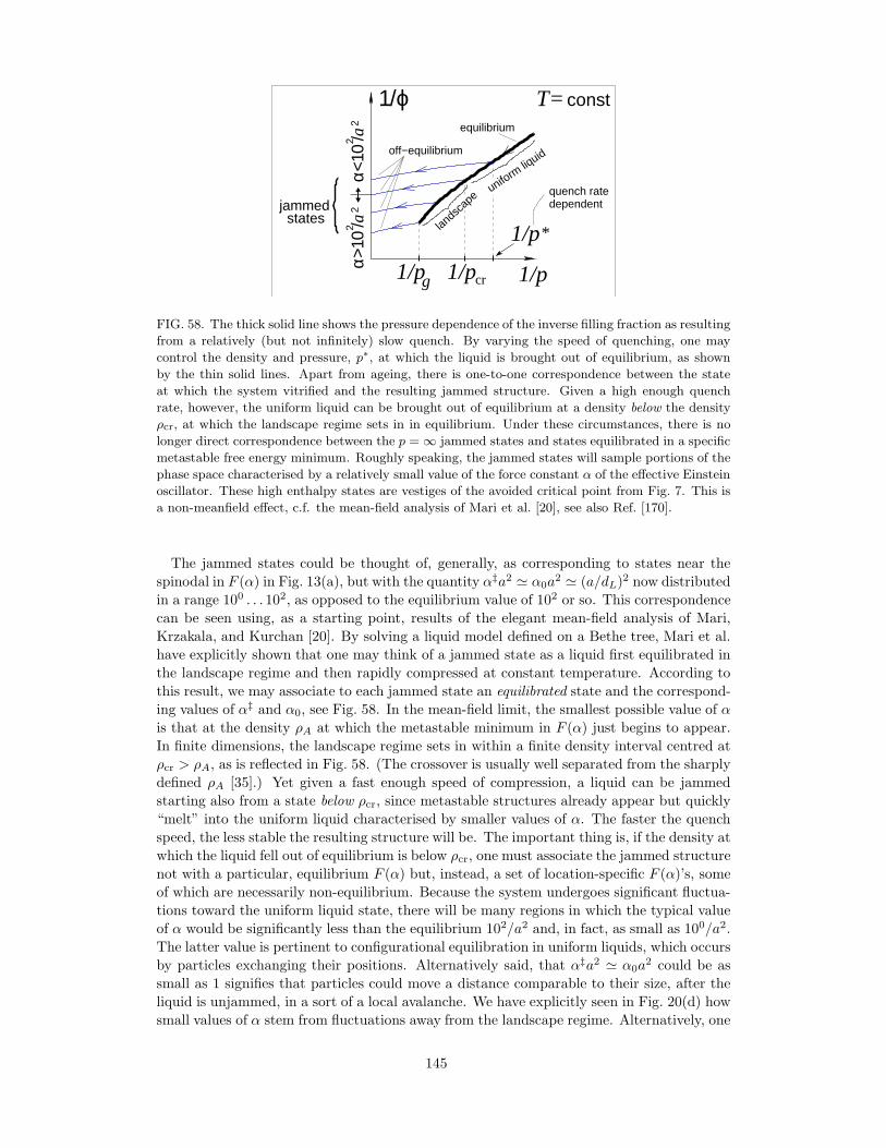
1/p*states

jammed

constT=

22

aα>

10 /

α<10

/2a

2

1/ϕ

g1/p 1/p

uniform

liquidoff−equilibrium

lands

cape

quench ratedependent

equilibrium

1/pcr

FIG. 58. The thick solid line shows the pressure dependence of the inverse filling fraction as resulting

from a relatively (but not infinitely) slow quench. By varying the speed of quenching, one may

control the density and pressure, p∗, at which the liquid is brought out of equilibrium, as shown

by the thin solid lines. Apart from ageing, there is one-to-one correspondence between the state

at which the system vitrified and the resulting jammed structure. Given a high enough quench

rate, however, the uniform liquid can be brought out of equilibrium at a density below the density

ρcr, at which the landscape regime sets in in equilibrium. Under these circumstances, there is no

longer direct correspondence between the p = ∞ jammed states and states equilibrated in a specific

metastable free energy minimum. Roughly speaking, the jammed states will sample portions of the

phase space characterised by a relatively small value of the force constant α of the effective Einstein

oscillator. These high enthalpy states are vestiges of the avoided critical point from Fig. 7. This is

a non-meanfield effect, c.f. the mean-field analysis of Mari et al. [20], see also Ref. [170].

The jammed states could be thought of, generally, as corresponding to states near the

spinodal in F (α) in Fig. 13(a), but with the quantity α‡a2 ≃ α0a2 ≃ (a/dL)

2 now distributed

in a range 100 . . . 102, as opposed to the equilibrium value of 102 or so. This correspondence

can be seen using, as a starting point, results of the elegant mean-field analysis of Mari,

Krzakala, and Kurchan [20]. By solving a liquid model defined on a Bethe tree, Mari et al.

have explicitly shown that one may think of a jammed state as a liquid first equilibrated in

the landscape regime and then rapidly compressed at constant temperature. According to

this result, we may associate to each jammed state an equilibrated state and the correspond-

ing values of α‡ and α0, see Fig. 58. In the mean-field limit, the smallest possible value of α

is that at the density ρA at which the metastable minimum in F (α) just begins to appear.

In finite dimensions, the landscape regime sets in within a finite density interval centred at

ρcr > ρA, as is reflected in Fig. 58. (The crossover is usually well separated from the sharply

defined ρA [35].) Yet given a fast enough speed of compression, a liquid can be jammed

starting also from a state below ρcr, since metastable structures already appear but quickly

“melt” into the uniform liquid characterised by smaller values of α. The faster the quench

speed, the less stable the resulting structure will be. The important thing is, if the density at

which the liquid fell out of equilibrium is below ρcr, one must associate the jammed structure

not with a particular, equilibrium F (α) but, instead, a set of location-specific F (α)’s, some

of which are necessarily non-equilibrium. Because the system undergoes significant fluctua-

tions toward the uniform liquid state, there will be many regions in which the typical value

of α would be significantly less than the equilibrium 102/a2 and, in fact, as small as 100/a2.

The latter value is pertinent to configurational equilibration in uniform liquids, which occurs

by particles exchanging their positions. Alternatively said, that α‡a2 ≃ α0a2 could be as

small as 1 signifies that particles could move a distance comparable to their size, after the

liquid is unjammed, in a sort of a local avalanche. We have explicitly seen in Fig. 20(d) how

small values of α stem from fluctuations away from the landscape regime. Alternatively, one

145

may think of such fluctuations as arising from local reduction in dimensionality, according

to Eq. (83).

The smallness of the effective α is a key difference between a jammed and vitrified system.

We reiterate that because the system is off-equilibrium, there is no intrinsic relation between

the stiffness of the jammed system and the value of α0 of the type from Eq. (30); the stiffness

becomes infinitely high in the p→ ∞ limit whereas α0 remains finite. Said in simpler terms,

the spacing between (vibrating) particles in contact, in a jammed structure, can be made

arbitrarily small while the structure remains practically the same. The particle displacement

upon unjamming, which is largely determined by the structure, is thus decoupled from the

vibrational motions.

Now take the zero temperature limit. Because the system is confined to an individual

free energy minimum at T = 0, before it escapes to a much lower enthalpy state, the

correlations should be mean-field like. This implies, among other things, that the relaxation

time should scale quadratically with the correlation length, τ ∝ ξ2A, as follows from the

mean-field Onsager-Landau ansatz for the relaxation of the pertinent order parameter φ:

φ ∝ −δF/δφ and Eq. (3). Given the decoupling between thermal vibration and density,

it is convenient to choose the filling fraction as the order parameter. Now, the scaling

ξA ∼ |φA − φ|−1/4 applies near a mean-field spinodal [348], where φA is the location of

the metastable minimum. Thus we obtain τ ∝ |φA − φ|−1/2. This is consistent with the

ω∗ ∝ |φA − φ|1/2 scaling discussed in Refs. [19, 349], where ω∗ is the infra-red edge of

stable harmonic modes, and also with recent unjamming simulations of soft spheres by

Ikeda, Berthier, and Biroli [350], in the low temperature limit. Although reasonable, the

above discussion is clearly qualitative and, certainly, is not a full-fledged field theory. Such

a field theory would have to contain exponentially many order parameters and appears

to be a complicated undertaking. Some progress toward obtaining such a field-theoretical

description of the landscape regime in finite dimensions has been achieved recently with the

help of replica techniques, see Refs. [209, 351] for instance.

In light of our earlier statements that the quantity α0a2 reflects the sharpness of the

first order transition from liquid to solid, we may conclude that, in fact, the lower density

jammed states are vestiges of an avoided critical point. That the critical point is destroyed

in equilibrium, means in thermodynamic terms that the critical fluctuations correspond to

higher free energy states. (Sometimes, such high free energy states may still correspond to

conditional equilibrium, such as the liquid-liquid separation in protein solutions mentioned

in Subsection IVB.) We have argued in Subsection III A that the critical point is pushed

down to zero temperature, which implies the solid formed as a result of the continuous

transition would be only marginally stable. And indeed, jammed systems are effectively zero

temperature. Long-range, critical correlations are destroyed by fluctuations in equilibrium,

but would be present in jammed systems which are not allowed to equilibrate. In fact, we

just saw that a diverging lengthscale appears during unjamming at low temperatures.

We thus conclude that there is a continuum of jammed states. The states from the more

stable, higher density part of this continuum are generated by quenching a liquid starting

at a density above ρcr, i.e., from a state that was fully equilibrated in the landscape regime.

In other words, the starting structure is trapped in a relatively well-defined free energy

minimum. The resulting jammed structure is hyperstatic. It appears that while being

jammed, such hyperstatic structures could exhibit additional, replica-symmetry breaking

transitions [352, 353] that are similar to the so called Gardner transitions in mean-field

spin glasses [354]. It is quite possible that in finite dimensions, these additional symmetry-

breaking transitions have to do with freezing out the residual string-like excitations that

would be characteristic of the crossover to the landscape regime. In contrast, the lower

density states from the continuum of jammed states can be traced to the very critical point

that is avoided when the system undergoes an equilibrium, discontinuous transition to the

146

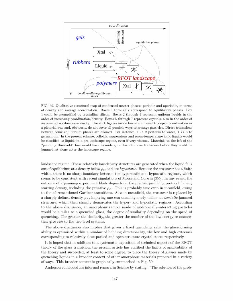
thre

sho

ld

equilibrium phases

conditionally−equilibruumstates

coordination

de

nsi

tyrubbers

gels

RFOT landscape

jam

min

g

polymers6

7

1

Xtal

Liquid

Xtal

23

4

5

FIG. 59. Qualitative structural map of condensed matter phases, periodic and aperiodic, in terms

of density and average coordination. Boxes 1 through 7 correspond to equilibrium phases. Box

1 could be exemplified by crystalline silicon. Boxes 2 through 4 represent uniform liquids in the

order of increasing coordination/density. Boxes 5 through 7 represent crystals, also in the order of

increasing coordination/density. The stick figures inside boxes are meant to depict coordination in

a pictorial way and, obviously, do not cover all possible ways to arrange particles. Direct transitions

between some equilibrium phases are allowed. For instance, 1 ↔ 2 pertains to water, 1 ↔ 3 to

germanium. In the present scheme, colloidal suspensions and room-temperature ionic liquids would

be classified as liquids in a pre-landscape regime, even if very viscous. Materials to the left of the

“jamming threshold” line would have to undergo a discontinuous transition before they could be

jammed let alone enter the landscape regime.

landscape regime. These relatively low-density structures are generated when the liquid falls

out of equilibrium at a density below ρcr and are hypostatic. Because the crossover has a finite

width, there is no sharp boundary between the hyperstatic and hypostatic regimes, which

seems to be consistent with recent simulations of Morse and Corwin [355]. In any event, the

outcome of a jamming experiment likely depends on the precise quenching protocol for any

starting density, including the putative ρK . This is probably true even in meanfield, owing

to the aforementioned Gardner transitions. Also in meanfield, the crossover is replaced by

a sharply defined density ρA, implying one can unambiguously define an isostatic jammed

structure, which then sharply demarcates the hyper- and hypostatic regimes. According

to the above discussion, an amorphous sample made of isotropically-interacting particles

would be similar to a quenched glass, the degree of similarity depending on the speed of

quenching. The greater the similarity, the greater the number of the low-energy resonances

that give rise to the two-level systems.

The above discussion also implies that given a fixed quenching rate, the glass-forming

ability is optimised within a window of bonding directionality, the low and high extremes

corresponding to relatively close-packed and open-structure crystal states respectively.

It is hoped that in addition to a systematic exposition of technical aspects of the RFOT

theory of the glass transition, the present article has clarified the limits of applicability of

the theory and succeeded, at least to some degree, to place the theory of glasses made by

quenching liquids in a broader context of other amorphous materials prepared in a variety

of ways. This broader context is graphically summarised in Fig. 59.

Anderson concluded his informal remark in Science by stating: “The solution of the prob-

147

|

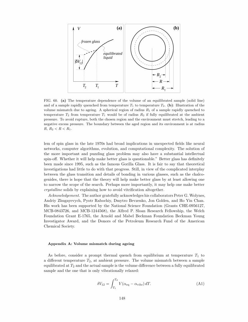
R2

R

12Vδ

V

T12 R1T T

equilibratedliquid

frozen glass

(a) (b)

|

FIG. 60. (a) The temperature dependence of the volume of an equilibrated sample (solid line)

and of a sample rapidly quenched from temperature T1 to temperature T2. (b): Illustration of the

volume mismatch due to ageing. A spherical region of radius R1 of a sample rapidly quenched to

temperature T2 from temperature T1 would be of radius R2 if fully equilibrated at the ambient

pressure. To avoid rupture, both the chosen region and the environment must stretch, leading to a

negative excess pressure. The boundary between the aged region and its environment is at radius

R, R2 < R < R1.

lem of spin glass in the late 1970s had broad implications in unexpected fields like neural

networks, computer algorithms, evolution, and computational complexity. The solution of

the more important and puzzling glass problem may also have a substantial intellectual

spin-off. Whether it will help make better glass is questionable.” Better glass has definitely

been made since 1995, such as the famous Gorilla Glass. It is fair to say that theoretical

investigations had little to do with that progress. Still, in view of the complicated interplay

between the glass transition and details of bonding in various glasses, such as the chalco-

genides, there is hope that the theory will help make better glass by at least allowing one

to narrow the scope of the search. Perhaps more importantly, it may help one make better

crystalline solids by explaining how to avoid vitrification altogether.

Acknowledgement. The author gratefully acknowledges his collaborators Peter G.Wolynes,

Andriy Zhugayevych, Pyotr Rabochiy, Dmytro Bevzenko, Jon Golden, and Ho Yin Chan.

His work has been supported by the National Science Foundation (Grants CHE-0956127,

MCB-0843726, and MCB-1244568), the Alfred P. Sloan Research Fellowship, the Welch

Foundation Grant E-1765, the Arnold and Mabel Beckman Foundation Beckman Young

Investigator Award, and the Donors of the Petroleum Research Fund of the American

Chemical Society.

Appendix A: Volume mismatch during ageing

As before, consider a prompt thermal quench from equilibrium at temperature T1 to

a different temperature T2, at ambient pressure. The volume mismatch between a sample

equilibrated at T2 and the actual sample is the volume difference between a fully equilibrated

sample and the one that is only vibrationally relaxed:

δV12 =

∫ T2

T1

V (αeq − αvibr) dT. (A1)

148

For concreteness, let us consider a downward T -jump: T2 < T1 ⇒ δV12 < 0, see illustration

in Fig. 60(a). Suppose a spherical region is of radius R1 before it structurally relaxed, at

the ambient pressure and temperature, and would be of radius R2 < R1 after relaxation, if

also at the ambient pressure and temperature. In view of the smallness of δV12/V (usually

not exceeding a few thousandth), δR/R ≡ (R2 −R1)/R ≈ δV12/3V , where R stands for the

actual radius of the droplet upon reconfiguration. To avoid fracture, both the inner and

outer regions must stretch (R2 < R < R1), see Fig. 60(b), leading to an excess negative

pressure p(r) throughout the sample. This pressure is constant within the reconfigured

region; it decreases away from the region and vanishes strictly at the external boundary of the

sample: p(∞) = 0. The excess pressure can be straightforwardly related to the deformation

using a solved problem from Chapter 7 of Ref. [85], assuming, for simplicity, isotropic

elasticity and a (macroscopic) spherical sample. At the boundary of the reconfigured region,

R − R2 = −p(R)R2/3Kin and R − R1 = p(R)R1/4µout where Kin is the equilibrium bulk

modulus at T2 and the ambient pressure, while µout the shear modulus of an individual

aperiodic state, also at T2 and ambient pressure. Excluding R, we find:

p(R) =δV12V

(1

Kin+

3

4µout

)−1

. (A2)

To estimate this excess pressure, p ∼ (δV12/V )µ/2, we note that for a realistic quench,

|δV12/V | . 5·10−3 [356], while the rule of thumb for elastic constants is µ(Tcr)a3 ≃ 12kBTcr,

see Eq. (208). And so, generically, µ(Tg)a3 ≃ 20kBTg, since Tg < Tcr, while µ usually

increases with lowering temperature. As a result, the excess pressure is comparable to but

probably less than |δV12/V |20kBT/a3. The latter does not exceed 10−1kBT/a3, which is

greater than the atmospheric pressure by a couple of orders of magnitude, but is comparably

less than the kinetic pressure. The latter is the relevant pressure reference here; its numerical

value is about (kBT/a3)(a/dL) ∼ 10kBT/a

3 [37, 170], see Subsection VC.

The environmental deformation, as a function of the radius vector r, is given by [85]

u(r) = (r/r3) p(R)R3/4µout (r > R). (A3)

The resulting volume change of the sample is 4π × p(R)R3/4µout, yielding for the relative

volume change of the whole sample:

δV

V

∣∣∣∣sample

=δV12V

(1 +

4µout

3Kin

)−1

(A4)

Note this total volume change takes place even as the environmental deformation from

Eq. (A3) is pure shear: ∇u ≡ uii = 0.

Also of potential interest is the free energy excess due to the deformation of the environ-

ment, which can be estimated by integrating the standard expression for the free energy

density over space, assuming again the isotropic elasticity and remembering that uii = 0 for

r > R:∫∞R

(µoutu2ik)4πr

2dr. This yields for the excess energy:

Eexc =πp(R)2

2µoutR3, (A5)

where p(R) is from Eq. (A2). Note this energy scales with the volume of the droplet. As

expected, there would not be any excess pressure or stored energy, if the material around

the nucleus could flow, in which case µout = 0 (p ∝ µout for µout → 0, by Eq. (A2)). Finally

note that formulae (A2)-(A5) apply for a δV12 of either sign, i.e., for both downward and

upward T -jumps. The physical difference between the two cases is that the excess pressure

p will be negative and positive for downward and upward jumps respectively.

149

It is apparent from Eq. (A4) that, owing to the shear resistance of the sample, the relative

volume change of the sample is always smaller than that of the reconfiguring (microscopic)

sub-regions, since the r.h.s. of Eq. (A4) is less than δV12/V , as long as µout > 0. This

would seemingly imply that the sample will never reach its equilibrium volume! There

is no contradiction here, however. As the sample equilibrates, i.e., the ageing proceeds,

the assumption of the mechanical stability is no longer valid. Hereby the material relaxes

throughout, all stored excess energy from Eq. (A5) is released, as recently described in

Ref. [47], while the shear modulus µout that enters in Eq. (A4) effectively decreases and

vanishes upon complete equilibration. Note that to achieve the latter, regions that originally

relaxed at a non-zero excess pressure p, will also have to relax until they are in equilibrium

at p = 0.

To quantify the significance of the volume-mismatch effect for the thermodynamics of

ageing we first note the stabilisation of state 2 from Eq. (216), per particle, is approximately

δ∆g ≃ (V p)/N = pa3, where we have used the usual expression for the Gibbs energy

increment: dG = −SdT + V dp. Together with Eq. (A2), this yields

δ∆g =δV12V

(1

Kin+

3

4µout

)−1

a3. (A6)

We thus observe that initial ageing events always overshoot in the following sense: For

downward T -jumps, the final state free energy is lower than the equilibrium free energy at

the ambient pressure (δV12 < 0) and vice versa for upward T -jumps (δV12 > 0).

To get a quantitative sense of this overshoot, let us adopt δ∆g ≃ (δV12/V )µa3/2 for the

sake of argument. As in the above estimate for the excess pressure, the stabilisation for

the δV12/V = −1 . . .5 · 10−3 range thus corresponds to δ∆g ≈ −0.01 . . .0.05kBT . This

stabilisation will be partially offset by the excess elastic energy stored in the environment,

from Eq. (A5): Eexc/N ≃ (3/8)p2a3/µout ≃ +0.1 · (δV12/V )2µa3, however the offset is

second order in the volume mismatch and sub-dominant by several orders of magnitude to

the main effect.

To quantify the effects of the overshoot caused by the volume-mismatch on the kinetics

of ageing, we note the free energy difference ∆g itself is about −0.9kBT at equilibrium

just above the glass transition on 1 hr time scale, according to Eq. (164) and using 1 psec

for the rate prefactor. For quenches below the glass transition: T1 = Tg, T2 < T1, ∆g is

only weakly T -dependent and predicted to decrease somewhat by absolute value [40], see

Eq. (217). Assuming for the sake of argument ∆f = −0.8kBT (i.e., a relaxation time of 105

s) one gets, upon replacing ∆g = −0.8kBT by ∆g = −0.85kBT , a speed up by a factor of ten

or so. Note that the thermal expansivity and the elastic moduli tend to anti-correlate [105],

and so the combination δV12µ, for similar quench depths, should not vary wildly among

different substances.

We have thus established that as regards thermodynamics and kinetics of ageing, the

volume-mismatch effect is quantitatively, but not qualitatively significant. One possible

exception is melting of ultrastable glasses, where the volume mismatch could exceed one

percent [261], thus leading to a relatively large δ∆g.

[1] I. Liritzis and C. Stevenson, Obsidian and Ancient Manufactured Glasses, University of New

Mexico Press, Albuquerque, 2012.

[2] J. Schroers, Physics Today 66 (2013), pp. 32–37.

[3] S. Raoux, W. We lnic, and D. Ielmini, Chem. Rev. 110 (2010), pp. 240–267.

[4] M. Wuttig and N. Yamada, Nature Mat. 6 (2007), pp. 824–832.

[5] D. Lencer, M. Salinga, B. Grabowski, T. Hickel, J. Neugebauer, and M. Wuttig, Nature Mat.

7 (2008), pp. 972–977.

150

[6] A.V. Kolobov, P. Fons, A.I. Frenkel, A.L. Ankudinov, J. Tominaga, and T. Uruga, Nature

Mat. 3 (2004), pp. 703–708.

[7] C. Steimer, V. Coulet, W. Welnic, H. Dieker, R. Detemple, C. Bichara, B. Beuneu, J. Gaspard,

and M. Wuttig, Adv. Mat. 20 (2008), pp. 4535–4540.

[8] P. Hosseini, C.D. Wright, and H. Bhaskaran, Nature 511 (2014), pp. 206–211.

[9] Y. Li, Y. Zhong, J. Zhang, L. Xu, Q. Wang, H. Sun, H. Tong, X. Cheng, and X. Miao, Sci.

Rep. 4 (2014), p. 4906.

[10] N.W. Ashcroft and N.D. Mermin, Solid State Physics, Harcourt Brace College Publishers,

Fort Worth, 1976.

[11] E. Leutheusser, Phys. Rev. A 29 (1984), p. 2765.

[12] U. Bengtzelius, W. Gotze, and A. Sjolander, J. Phys. C: Solid State Physics 17 (1984), pp.

5915–5934.

[13] A.S. Keys, J.P. Garrahan, and D. Chandler, Proc. Natl. Acad. Sci. U. S. A. 110 (2013), pp.

4482–4487.

[14] A.S. Keys, L.O. Hedges, J.P. Garrahan, S.C. Glotzer, and D. Chandler, Phys. Rev. X 1 (2011),

p. 021013.

[15] R.G. Palmer, D.L. Stein, E. Abrahams, and P.W. Anderson, Phys. Rev. Lett. 53 (1984), pp.

958–961.

[16] G.H. Fredrickson and H.C. Andersen, Phys. Rev. Lett. 53 (1984), pp. 1244–1247.

[17] A.S. Keys, A.R. Abate, S.C. Glotzer, and D.J. Durian, Nature Physics 3 (2007), pp. 260–264.

[18] A.J. Liu and S.R. Nagel, Nature 395 (1998), pp. 21–22.

[19] L.S. Silbert, A.J. Liu, and S.R. Nagel, Phys. Rev. Lett. 95 (2005), p. 098301.

[20] R. Mari, F. Krzakala, and J. Kurchan, Phys. Rev. Lett. 103 (2009), p. 025701.

[21] T.S. Grigera, V. Martin-Mayor, G. Parisi, and P. Verrocchio, Nature 422 (2003), pp. 289–292.

[22] V. Lubchenko and P.G. Wolynes, Proc. Natl. Acad. Sci. U. S. A. 100 (2003), pp. 1515–1518.

[23] V. Lubchenko and P.G. Wolynes, Adv. Chem. Phys. 136 (2007), pp. 95–206.

[24] L. Onsager, Phys. Rev. 37 (1931), pp. 405–426.

[25] L. Onsager, Phys. Rev. 38 (1931), pp. 2265–2279.

[26] N. Goldenfeld, Lectures on phase transitions and the renormalization group, Addison-Wesley,

Reading, MA, 1992.

[27] V. Lubchenko and P.G. Wolynes, Annu. Rev. Phys. Chem. 58 (2007), pp. 235–266.

[28] V. Lubchenko, J. Phys. Chem. Lett. 3 (2012), pp. 1–7.

[29] A. Zhugayevych and V. Lubchenko, J. Chem. Phys. 133 (2010), p. 234503.

[30] T.R. Kirkpatrick, D. Thirumalai, and P.G. Wolynes, Phys. Rev. A 40 (1989), pp. 1045–1054.

[31] X. Xia and P.G. Wolynes, Proc. Natl. Acad. Sci. U. S. A. 97 (2000), pp. 2990–2994.

[32] P. Rabochiy and V. Lubchenko, J. Chem. Phys. 138 (2013), 12A534.

[33] P. Rabochiy, P.G. Wolynes, and V. Lubchenko, J. Phys. Chem. B 117 (2013), pp. 15204–15219.

[34] V. Lubchenko and P. Rabochiy, J. Phys. Chem. B 118 (2014), pp. 13744–13759.

[35] V. Lubchenko and P.G. Wolynes, J. Chem. Phys. 119 (2003), pp. 9088–9105.

[36] J. Stevenson and P.G. Wolynes, J. Phys. Chem. B 109 (2005), pp. 15093–15097.

[37] P. Rabochiy and V. Lubchenko, J. Chem. Phys. 136 (2012), p. 084504.

[38] X. Xia and P.G. Wolynes, Phys. Rev. Lett. 86 (2001), pp. 5526–5529.

[39] X. Xia and P.G. Wolynes, J. Phys. Chem. 105 (2001), pp. 6570–6573.

[40] V. Lubchenko and P.G. Wolynes, J. Chem. Phys. 121 (2004), pp. 2852–2865.

[41] J.D. Stevenson, J. Schmalian, and P.G. Wolynes, Nature Physics 2 (2006), pp. 268–274.

[42] P. Rabochiy and V. Lubchenko, J. Phys. Chem. B 116 (2012), pp. 5729–5737.

[43] V. Lubchenko, J. Chem. Phys. 126 (2007), p. 174503.

[44] J.D. Stevenson and P.G. Wolynes, Nature Physics 6 (2010), pp. 62–68.

[45] V. Lubchenko, Proc. Natl. Acad. Sci. U. S. A. 106 (2009), pp. 11506–11510.

[46] J.D. Stevenson and P.G. Wolynes, J. Chem. Phys. 129 (2008), p. 234514.

[47] A. Wisitsorasak and P.G. Wolynes, Proc. Natl. Acad. Sci. U. S. A. 109 (2012), pp. 16068–

16072.

[48] P.G. Wolynes, Proc. Natl. Acad. Sci. U. S. A. 106 (2009), pp. 1353–1358.

[49] A. Wisitsorasak and P.G. Wolynes, Phys. Rev. E 88 (2013), p. 022308.

[50] J.D. Stevenson and P.G. Wolynes, J. Phys. Chem. A 115 (2011), pp. 3713–3719.

[51] V. Lubchenko and P.G. Wolynes, Phys. Rev. Lett. 87 (2001), p. 195901.

151

[52] V. Lubchenko, R.J. Silbey, and P.G. Wolynes, Mol. Phys. 104 (2006), pp. 1325–1335.

[53] A. Zhugayevych and V. Lubchenko, J. Chem. Phys. 132 (2010), p. 044508.

[54] A. Zhugayevych and V. Lubchenko, J. Chem. Phys. 133 (2010), p. 234504.

[55] L.D. Landau and E.M. Lifshitz, Statistical Mechanics, Pergamon Press, New York, 1980.

[56] R.S. Berry, S.A. Rice, and J. Ross, Physical Chemistry, John Wiley & Sons, Hoboken, NJ,

1980.

[57] W.M. Haynes (ed.), CRC Handbook of Chemistry and Physics, 96th Edition, CRC Press, Boca

Raton, 2015.

[58] O. Penrose, J. Stat. Phys. 78 (1995), pp. 267–283.

[59] T. Hikima, Y. Adachi, M. Hanaya, and M. Oguni, Phys. Rev. B 52 (1995), pp. 3900–3908.

[60] Y. Sun, H. Xi, S. Chen, M.D. Ediger, and L. Yu, J. Phys. Chem. B 112 (2008), pp. 5594–5601.

[61] C.A. Angell, Science 267 (1995), pp. 1924–1935, Available at

http://www.jstor.org/stable/2886440.

[62] P. Lunkenheimer, M. Kohler, S. Kastner, and A. Loidl, Dielectric spectroscopy of glassy dy-

namics, in Structural Glasses and Supercooled Liquids: Theory, Experiment, and Applications,

P.G. Wolynes and V. Lubchenko, eds., John Wiley & Sons, Hoboken, NJ (2012), pp. 115–149.

[63] M. Born and K. Huang, Dynamic Theory of Crystal Lattices, Oxford, Clarendon Press, 1968.

[64] N.F. Mott and R.W. Gurney, Trans. Faraday Soc. 35 (1939), pp. 364–368.

[65] V. Lubchenko, J. Phys. Chem. B 110 (2006), pp. 18779–18786.

[66] J. Daeges, H. Gleiter, and J. Perepezko, Phys. Lett. A 119 (1986), pp. 79 – 82.

[67] J.H. Bilgram, Phys. Rep. 153 (1987), pp. 1–89.

[68] S.R. Philpot, S. Yip, P.R. Okamoto, and D. Wolf, Role of interfaces in melting and solid-state

amorphization, in Materials Interfaces: Atomic-level Structure and Properties, D. Wolf and

S. Yip, eds., Springer, New York (1992), pp. 228–254.

[69] A.P. Young, Phase Diagrams of the Elements, Lawrence Livermore Laboratory, University of

California, Livermore, CA, 1975.

[70] J.E. Lennard-Jones and A.F. Devonshire, Proceedings of the Royal Society of London. Series

A 163 (1937), pp. pp. 53–70.

[71] J. Hirschfelder, D. Stevenson, and H. Eyring, J. Chem. Phys. 5 (1937), pp. 896–912.

[72] W.G. Hoover and F.H. Ree, J. Chem. Phys. 49 (1968), pp. 3609–3617.

[73] M. Fixman, J. Chem. Phys. 51 (1969), pp. 3270–3279.

[74] J.D. Bernal, Trans. Faraday Soc. 33 (1937), pp. 27–40.

[75] L. Landau, Phys. Z. Sowjet. 11 (1937), p. 26, English translation in ”Collected Papers of

Landau”, 1965, Gordon and Breach.

[76] L. Landau, Phys. Z. Sowjet. 11 (1937), p. 545, English translation in ”Collected Papers of

Landau”, 1965, Gordon and Breach.

[77] R.J. Baxter, J. Chem. Phys. 41 (1964), pp. 553–558.

[78] J.P. Hansen and I.R. McDonald, Theory of Simple Liquids, Academic Press, New York, 1976.

[79] R. Evans, Adv. Phys. 28 (1979), pp. 143–200.

[80] P. Hohenberg and W. Kohn, Phys. Rev. 136 (1964), pp. B864–B871.

[81] N.D. Mermin, Phys. Rev. 137 (1965), pp. A1441–A1443.

[82] J.S. McCarley and N.W. Ashcroft, Phys. Rev. E 55 (1997), pp. 4990–5003.

[83] D. Henderson and E.W. Grundke, J. Chem. Phys. 63 (1975), pp. 601–607.

[84] S. Asakura and F. Oosawa, J. Polymer Sci. 33 (1958), pp. 183–193.

[85] L.D. Landau and E.M. Lifshitz, Theory of Elasticity, Pergamon Press, 1986.

[86] A.C. Eringen and D.G.B. Edelen, Int. J. Engrg. Sci. 10 (1972), p. 233.

[87] I.A. Kunin, Elastic Media with Microstructure, Springer, New York, 1982.

[88] K.C. Valanis, Arch. Mech. 52 (2000), pp. 817–838.

[89] A.J.M. Yang, P.D. Fleming, and J.H. Gibbs, J. Chem. Phys. 64 (1976), pp. 3732–3747.

[90] S. Alexander and J. McTague, Phys. Rev. Lett. 41 (1978), pp. 702–705.

[91] P.W. Anderson, Basic Notions of Condensed Matter Physics, Benjamin Cummins, 1984.

[92] T.C. Hales, Notices Amer. Math. Soc. 47 (2000), pp. 440–449.

[93] S.A. Brazovskii, JETP 41 (1975), pp. 85–89.

[94] S.A. Brazovskii and S.G. Dmitriev, JETP 42 (1975), pp. 497–502.

[95] J. Frohlich and T. Spencer, Commun. Math. Phys. 84 (1982), pp. 87–101.

[96] P.W. Anderson and G. Yuval, J. Phys. C 4 (1971), pp. 607–620.

152

[97] P.M. Chaikin and T.C. Lubensky, Principles of Condensed Matter Physics, Cambridge Uni-

versity Press, Cambridge, 2000.

[98] M.I. McMahon and R.J. Nelmes, Chem. Soc. Rev. 35 (2006), pp. 943–963.

[99] H. Olijnyk and W. Holzapfel, Phys. Lett. A 100 (1984), pp. 191 – 194.

[100] D. Legut, M. Friak, and M. Sob, Phys. Rev. Lett. 99 (2007), p. 016402.

[101] S.M. Woodley and R. Catlow, Nature Materials 7 (2008), pp. 937 – 946.

[102] J.G. Kirkwood and E. Monroe, The Journal of Chemical Physics 9 (1941), pp. 514–526.

[103] V.N. Ryzhov and E.E. Tareeva, Theor. Mat. Phys. (USSR) 48 (1981), pp. 835–840.

[104] S.A. Rice, C. Cerjan, and B. Bagchi, J. Chem. Phys. 82 (1985), pp. 3350–3359.

[105] G. Grimvall and S. Sjodin, Phys. Scripta 10 (1974), p. 340.

[106] M. Mezard and G. Parisi, Phys. Rev. Lett. 82 (1999), pp. 747–750.

[107] F.A. Lindemann, Phys. Z. 11 (1910), pp. 609–612.

[108] J.D. van der Waals, Over de Continuitet van der Gas- en Vloeistoftoestand, Ph.D. thesis,

Univ. Leiden, 1873, english translation: Phys. Mem., vol. 1, p. 333, 1890.

[109] P. Weiss, J. Phys. Theor. Appl. 6 (1907), pp. 661–690.

[110] D.M. McQuarrie, Statistical Mechanics, Harper-Collins, New York, 1973.

[111] H.B. Callen, Thermodynamics and an Introduction to Thermostatistics, Wiley, Hoboken, NJ,

1985.

[112] R. Lovett, C.Y. Mou, and F.P. Buff, J. Chem. Phys. 65 (1976), pp. 570–572.

[113] A.D.J. Haymet and D.W. Oxtoby, J. Chem. Phys. 74 (1981), pp. 2559–2565.

[114] L.D. Landau and E.M. Lifshitz, Mechanics, Pergamon Press, New York, 1976.

[115] T.V. Ramakrishnan and M. Yussouff, Phys. Rev. B 19 (1979), pp. 2775–2794.

[116] M.S. Wertheim, J. Chem. Phys. 65 (1976), pp. 2377–2381.

[117] R. Lovett, J. Chem. Phys. 66 (1977), pp. 1225–1230.

[118] J.K. Percus and G.J. Yevick, Phys. Rev. 110 (1958), pp. 1–13.

[119] E. Thiele, J. Chem. Phys. 39 (1963), pp. 474–479.

[120] M.S. Wertheim, Phys. Rev. Lett. 10 (1963), pp. 321–323.

[121] W.L. Bragg and E.J. Williams, Proc. Roy. Soc. A145 (1934), pp. 699–730.

[122] R. Feynman, Statistical Mechanics: A Set Of Lectures, Advanced Books Classics Series, West-

view Press, Boulder, CO, 1998.

[123] L. Onsager, Ann. N. Y. Acad. Sci. 51 (1949), pp. 627–659.

[124] J.L. Lebowitz and J.K. Percus, J. Math. Phys. 4 (1963), pp. 116–123.

[125] F.H. Stillinger, P.G. Debenedetti, and S. Sastry, J. Chem. Phys. 109 (1998), pp. 3983–3988.

[126] L.S. Ornstein and F. Zernike, Proc. Acad. Sci. Amsterdam 17 (1914), pp. 793–806, reproduced

in H. Frisch and J. L. Lebowitz, The Equilibrium Theory of Classical Fluids, Benjamin, 1964.

[127] M.P. Allen and D.J. Tildesley, Computer Simulation of Liquids, Oxford University Press,

USA, Oxford, 1989.

[128] M. Dixon and P. Hutchinson, Mol. Phys. 33 (1977), pp. 1663–1670.

[129] A.R. Denton and N.W. Ashcroft, Phys. Rev. A 39 (1989), p. 4701.

[130] H. Lowen, J. Phys.: Condens. Matter 2 (1990), pp. 8477–8484.

[131] J.L. Barrat, J.P. Hansen, G. Pastore, and E.M. Waisman, J. Chem. Phys. 86 (1987), pp.

6360–6365.

[132] W.A. Curtin and N.W. Ashcroft, Phys. Rev. Lett. 56 (1986), pp. 2775–2778.

[133] J.P. Hansen and L. Verlet, Phys. Rev. 184 (1969), pp. 151–161.

[134] B.W.H. van Beest, G.J. Kramer, and R.A. van Santen, Phys. Rev. Lett. 64 (1990), pp. 1955–

1958.

[135] J.H. Magill, J. Chem. Phys. 47 (1967), pp. 2802–2807.

[136] T.A. Albright, J.K. Burdett, and M.H. Whangbo, Orbital Interactions in Chemistry, Wiley,

Hoboken, NJ, 2013.

[137] G. Parisi and F. Zamponi, Rev. Mod. Phys. 82 (2010), pp. 789–845.

[138] S.M. Sharma and S. Sikka, Prog. Mater. Sci. 40 (1996), pp. 1 – 77.

[139] V.V. Brazhkin and A.G. Lyapin, J. Phys. Cond. Mat. 15 (2003), p. 6059.

[140] E. Ponyatovsky and O. Barkalov, Mat. Sci. Rep. 8 (1992), pp. 147 – 191.

[141] R.J. Hemley, A.P. Jephcoat, H.K. Mao, L.C. Ming, and M.H. Manghnani, Nature 334 (1988),

pp. 52–54.

[142] J.P. Stoessel and P.G. Wolynes, J. Chem. Phys. 80 (1984), pp. 4502–4512.

153

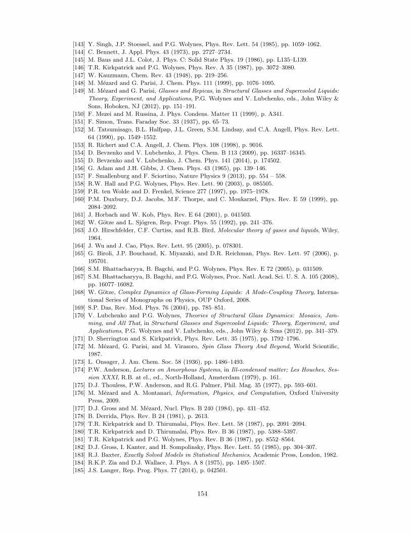
[143] Y. Singh, J.P. Stoessel, and P.G. Wolynes, Phys. Rev. Lett. 54 (1985), pp. 1059–1062.

[144] C. Bennett, J. Appl. Phys. 43 (1973), pp. 2727–2734.

[145] M. Baus and J.L. Colot, J. Phys. C: Solid State Phys. 19 (1986), pp. L135–L139.

[146] T.R. Kirkpatrick and P.G. Wolynes, Phys. Rev. A 35 (1987), pp. 3072–3080.

[147] W. Kauzmann, Chem. Rev. 43 (1948), pp. 219–256.

[148] M. Mezard and G. Parisi, J. Chem. Phys. 111 (1999), pp. 1076–1095.

[149] M. Mezard and G. Parisi, Glasses and Repicas, in Structural Glasses and Supercooled Liquids:

Theory, Experiment, and Applications, P.G. Wolynes and V. Lubchenko, eds., John Wiley &

Sons, Hoboken, NJ (2012), pp. 151–191.

[150] F. Mezei and M. Russina, J. Phys. Condens. Matter 11 (1999), p. A341.

[151] F. Simon, Trans. Faraday Soc. 33 (1937), pp. 65–73.

[152] M. Tatsumisago, B.L. Halfpap, J.L. Green, S.M. Lindsay, and C.A. Angell, Phys. Rev. Lett.

64 (1990), pp. 1549–1552.

[153] R. Richert and C.A. Angell, J. Chem. Phys. 108 (1998), p. 9016.

[154] D. Bevzenko and V. Lubchenko, J. Phys. Chem. B 113 (2009), pp. 16337–16345.

[155] D. Bevzenko and V. Lubchenko, J. Chem. Phys. 141 (2014), p. 174502.

[156] G. Adam and J.H. Gibbs, J. Chem. Phys. 43 (1965), pp. 139–146.

[157] F. Smallenburg and F. Sciortino, Nature Physics 9 (2013), pp. 554 – 558.

[158] R.W. Hall and P.G. Wolynes, Phys. Rev. Lett. 90 (2003), p. 085505.

[159] P.R. ten Wolde and D. Frenkel, Science 277 (1997), pp. 1975–1978.

[160] P.M. Duxbury, D.J. Jacobs, M.F. Thorpe, and C. Moukarzel, Phys. Rev. E 59 (1999), pp.

2084–2092.

[161] J. Horbach and W. Kob, Phys. Rev. E 64 (2001), p. 041503.

[162] W. Gotze and L. Sjogren, Rep. Progr. Phys. 55 (1992), pp. 241–376.

[163] J.O. Hirschfelder, C.F. Curtiss, and R.B. Bird, Molecular theory of gases and liquids, Wiley,

1964.

[164] J. Wu and J. Cao, Phys. Rev. Lett. 95 (2005), p. 078301.

[165] G. Biroli, J.P. Bouchaud, K. Miyazaki, and D.R. Reichman, Phys. Rev. Lett. 97 (2006), p.

195701.

[166] S.M. Bhattacharyya, B. Bagchi, and P.G. Wolynes, Phys. Rev. E 72 (2005), p. 031509.

[167] S.M. Bhattacharyya, B. Bagchi, and P.G. Wolynes, Proc. Natl. Acad. Sci. U. S. A. 105 (2008),

pp. 16077–16082.

[168] W. Gotze, Complex Dynamics of Glass-Forming Liquids: A Mode-Coupling Theory, Interna-

tional Series of Monographs on Physics, OUP Oxford, 2008.

[169] S.P. Das, Rev. Mod. Phys. 76 (2004), pp. 785–851.

[170] V. Lubchenko and P.G. Wolynes, Theories of Structural Glass Dynamics: Mosaics, Jam-

ming, and All That, in Structural Glasses and Supercooled Liquids: Theory, Experiment, and

Applications, P.G. Wolynes and V. Lubchenko, eds., John Wiley & Sons (2012), pp. 341–379.

[171] D. Sherrington and S. Kirkpatrick, Phys. Rev. Lett. 35 (1975), pp. 1792–1796.

[172] M. Mezard, G. Parisi, and M. Virasoro, Spin Glass Theory And Beyond, World Scientific,

1987.

[173] L. Onsager, J. Am. Chem. Soc. 58 (1936), pp. 1486–1493.

[174] P.W. Anderson, Lectures on Amorphous Systems, in Ill-condensed matter; Les Houches, Ses-

sion XXXI, R.B. at el., ed., North-Holland, Amsterdam (1979), p. 161.

[175] D.J. Thouless, P.W. Anderson, and R.G. Palmer, Phil. Mag. 35 (1977), pp. 593–601.

[176] M. Mezard and A. Montanari, Information, Physics, and Computation, Oxford University

Press, 2009.

[177] D.J. Gross and M. Mezard, Nucl. Phys. B 240 (1984), pp. 431–452.

[178] B. Derrida, Phys. Rev. B 24 (1981), p. 2613.

[179] T.R. Kirkpatrick and D. Thirumalai, Phys. Rev. Lett. 58 (1987), pp. 2091–2094.

[180] T.R. Kirkpatrick and D. Thirumalai, Phys. Rev. B 36 (1987), pp. 5388–5397.

[181] T.R. Kirkpatrick and P.G. Wolynes, Phys. Rev. B 36 (1987), pp. 8552–8564.

[182] D.J. Gross, I. Kanter, and H. Sompolinsky, Phys. Rev. Lett. 55 (1985), pp. 304–307.

[183] R.J. Baxter, Exactly Solved Models in Statistical Mechanics, Academic Press, London, 1982.

[184] R.K.P. Zia and D.J. Wallace, J. Phys. A 8 (1975), pp. 1495–1507.

[185] J.S. Langer, Rep. Prog. Phys. 77 (2014), p. 042501.

154

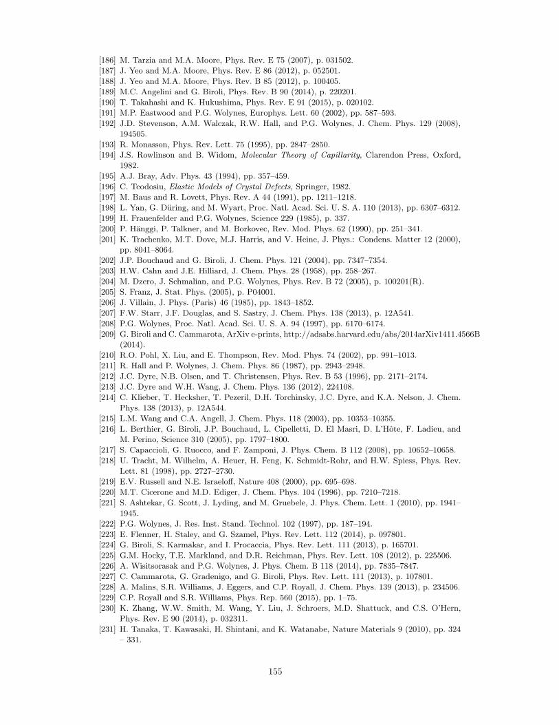
[186] M. Tarzia and M.A. Moore, Phys. Rev. E 75 (2007), p. 031502.

[187] J. Yeo and M.A. Moore, Phys. Rev. E 86 (2012), p. 052501.

[188] J. Yeo and M.A. Moore, Phys. Rev. B 85 (2012), p. 100405.

[189] M.C. Angelini and G. Biroli, Phys. Rev. B 90 (2014), p. 220201.

[190] T. Takahashi and K. Hukushima, Phys. Rev. E 91 (2015), p. 020102.

[191] M.P. Eastwood and P.G. Wolynes, Europhys. Lett. 60 (2002), pp. 587–593.

[192] J.D. Stevenson, A.M. Walczak, R.W. Hall, and P.G. Wolynes, J. Chem. Phys. 129 (2008),

194505.

[193] R. Monasson, Phys. Rev. Lett. 75 (1995), pp. 2847–2850.

[194] J.S. Rowlinson and B. Widom, Molecular Theory of Capillarity, Clarendon Press, Oxford,

1982.

[195] A.J. Bray, Adv. Phys. 43 (1994), pp. 357–459.

[196] C. Teodosiu, Elastic Models of Crystal Defects, Springer, 1982.

[197] M. Baus and R. Lovett, Phys. Rev. A 44 (1991), pp. 1211–1218.

[198] L. Yan, G. During, and M. Wyart, Proc. Natl. Acad. Sci. U. S. A. 110 (2013), pp. 6307–6312.

[199] H. Frauenfelder and P.G. Wolynes, Science 229 (1985), p. 337.

[200] P. Hanggi, P. Talkner, and M. Borkovec, Rev. Mod. Phys. 62 (1990), pp. 251–341.

[201] K. Trachenko, M.T. Dove, M.J. Harris, and V. Heine, J. Phys.: Condens. Matter 12 (2000),

pp. 8041–8064.

[202] J.P. Bouchaud and G. Biroli, J. Chem. Phys. 121 (2004), pp. 7347–7354.

[203] H.W. Cahn and J.E. Hilliard, J. Chem. Phys. 28 (1958), pp. 258–267.

[204] M. Dzero, J. Schmalian, and P.G. Wolynes, Phys. Rev. B 72 (2005), p. 100201(R).

[205] S. Franz, J. Stat. Phys. (2005), p. P04001.

[206] J. Villain, J. Phys. (Paris) 46 (1985), pp. 1843–1852.

[207] F.W. Starr, J.F. Douglas, and S. Sastry, J. Chem. Phys. 138 (2013), p. 12A541.

[208] P.G. Wolynes, Proc. Natl. Acad. Sci. U. S. A. 94 (1997), pp. 6170–6174.

[209] G. Biroli and C. Cammarota, ArXiv e-prints, http://adsabs.harvard.edu/abs/2014arXiv1411.4566B

(2014).

[210] R.O. Pohl, X. Liu, and E. Thompson, Rev. Mod. Phys. 74 (2002), pp. 991–1013.

[211] R. Hall and P. Wolynes, J. Chem. Phys. 86 (1987), pp. 2943–2948.

[212] J.C. Dyre, N.B. Olsen, and T. Christensen, Phys. Rev. B 53 (1996), pp. 2171–2174.

[213] J.C. Dyre and W.H. Wang, J. Chem. Phys. 136 (2012), 224108.

[214] C. Klieber, T. Hecksher, T. Pezeril, D.H. Torchinsky, J.C. Dyre, and K.A. Nelson, J. Chem.

Phys. 138 (2013), p. 12A544.

[215] L.M. Wang and C.A. Angell, J. Chem. Phys. 118 (2003), pp. 10353–10355.

[216] L. Berthier, G. Biroli, J.P. Bouchaud, L. Cipelletti, D. El Masri, D. L’Hote, F. Ladieu, and

M. Perino, Science 310 (2005), pp. 1797–1800.

[217] S. Capaccioli, G. Ruocco, and F. Zamponi, J. Phys. Chem. B 112 (2008), pp. 10652–10658.

[218] U. Tracht, M. Wilhelm, A. Heuer, H. Feng, K. Schmidt-Rohr, and H.W. Spiess, Phys. Rev.

Lett. 81 (1998), pp. 2727–2730.

[219] E.V. Russell and N.E. Israeloff, Nature 408 (2000), pp. 695–698.

[220] M.T. Cicerone and M.D. Ediger, J. Chem. Phys. 104 (1996), pp. 7210–7218.

[221] S. Ashtekar, G. Scott, J. Lyding, and M. Gruebele, J. Phys. Chem. Lett. 1 (2010), pp. 1941–

1945.

[222] P.G. Wolynes, J. Res. Inst. Stand. Technol. 102 (1997), pp. 187–194.

[223] E. Flenner, H. Staley, and G. Szamel, Phys. Rev. Lett. 112 (2014), p. 097801.

[224] G. Biroli, S. Karmakar, and I. Procaccia, Phys. Rev. Lett. 111 (2013), p. 165701.

[225] G.M. Hocky, T.E. Markland, and D.R. Reichman, Phys. Rev. Lett. 108 (2012), p. 225506.

[226] A. Wisitsorasak and P.G. Wolynes, J. Phys. Chem. B 118 (2014), pp. 7835–7847.

[227] C. Cammarota, G. Gradenigo, and G. Biroli, Phys. Rev. Lett. 111 (2013), p. 107801.

[228] A. Malins, S.R. Williams, J. Eggers, and C.P. Royall, J. Chem. Phys. 139 (2013), p. 234506.

[229] C.P. Royall and S.R. Williams, Phys. Rep. 560 (2015), pp. 1–75.

[230] K. Zhang, W.W. Smith, M. Wang, Y. Liu, J. Schroers, M.D. Shattuck, and C.S. O’Hern,

Phys. Rev. E 90 (2014), p. 032311.

[231] H. Tanaka, T. Kawasaki, H. Shintani, and K. Watanabe, Nature Materials 9 (2010), pp. 324

– 331.

155

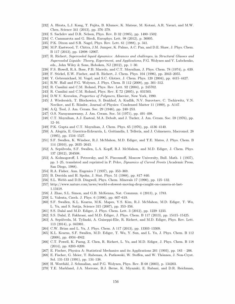
[232] A. Hirata, L.J. Kang, T. Fujita, B. Klumov, K. Matsue, M. Kotani, A.R. Yavari, and M.W.

Chen, Science 341 (2013), pp. 376–379.

[233] S. Sachdev and D.R. Nelson, Phys. Rev. B 32 (1985), pp. 1480–1502.

[234] C. Cammarota and G. Biroli, Europhys. Lett. 98 (2012), p. 36005.

[235] P.K. Dixon and S.R. Nagel, Phys. Rev. Lett. 61 (1988), p. 341.

[236] M.P. Eastwood, T. Chitra, J.M. Jumper, K. Palmo, A.C. Pan, and D.E. Shaw, J. Phys. Chem.

B 117 (2013), pp. 12898–12907.

[237] R. Richert, Supercooled liquid dynamics: Advances and challenges, in Structural Glasses and

Supercooled Liquids: Theory, Experiment, and Applications, P.G. Wolynes and V. Lubchenko,

eds., John Wiley & Sons, Hoboken, NJ (2012), pp. 1–30.

[238] F.S. Howell, R.A. Bose, P.B. Macedo, and C.T. Moynihan, J. Phys. Chem. 78 (1974), p. 639.

[239] F. Stickel, E.W. Fischer, and R. Richert, J. Chem. Phys. 104 (1996), pp. 2043–2055.

[240] Y. Gebremichael, M. Vogel, and S.C. Glotzer, J. Chem. Phys. 120 (2004), pp. 4415–4427.

[241] R.W. Hall and P.G. Wolynes, J. Phys. Chem. B 112 (2008), pp. 301–312.

[242] R. Casalini and C.M. Roland, Phys. Rev. Lett. 92 (2004), p. 245702.

[243] R. Casalini and C.M. Roland, Phys. Rev. E 72 (2005), p. 031503.

[244] D.W.V. Krevelen, Properties of Polymers, Elsevier, New York, 1990.

[245] J. Wiedersich, T. Blochowicz, S. Benkhof, A. Kudlik, N.V. Surovtsev, C. Tschirwitz, V.N.

Novikov, and E. Rossler, Journal of Physics: Condensed Matter 11 (1999), p. A147.

[246] A.Q. Tool, J. Am. Ceram. Soc. 29 (1946), pp. 240–253.

[247] O.S. Narayanaswamy, J. Am. Ceram. Soc. 54 (1971), pp. 491–498.

[248] C.T. Moynihan, A.J. Easteal, M.A. Debolt, and J. Tucker, J. Am. Ceram. Soc. 59 (1976), pp.

12–16.

[249] P.K. Gupta and C.T. Moynihan, J. Chem. Phys. 65 (1976), pp. 4136–4140.

[250] A. Alegrıa, E. Guerrica-Echvarrıa, L. Goitiandıa, I. Tellerıa, and J. Colmenero, Macromol. 28

(1995), pp. 1516–1527.

[251] S.F. Swallen, K. Windsor, R.J. McMahon, M.D. Ediger, and T.E. Mates, J. Phys. Chem. B

114 (2010), pp. 2635–2643.

[252] A. Sepulveda, S.F. Swallen, L.A. Kopff, R.J. McMahon, and M.D. Ediger, J. Chem. Phys.

137 (2012), 204508.

[253] A. Kolmogoroff, I. Petrovsky, and N. Piscounoff, Moscow University, Bull. Math. 1 (1937),

pp. 1–25, translated and reprinted in P. Pelce, Dynamics of Curved Fronts (Academic Press,

San Diego, 1988).

[254] R.A. Fisher, Ann. Eugenics 7 (1937), pp. 353–369.

[255] B. Derrida and H. Spohn, J. Stat. Phys. 51 (1988), pp. 817–840.

[256] S.L. Webb and D.B. Dingwell, Phys. Chem. Minerals 17 (1990), pp. 125–132.

[257] http://www.nature.com/news/world-s-slowest-moving-drop-caught-on-camera-at-last-

1.13418.

[258] J. Zhao, S.L. Simon, and G.B. McKenna, Nat. Commun. 4 (2013), p. 1783.

[259] L. Valenta, Czech. J. Phys. 6 (1996), pp. 607–619.

[260] S.F. Swallen, K.L. Kearns, M.K. Mapes, Y.S. Kim, R.J. McMahon, M.D. Ediger, T. Wu,

L. Yu, and S. Satija, Science 315 (2007), pp. 353–356.

[261] S.S. Dalal and M.D. Ediger, J. Phys. Chem. Lett. 3 (2012), pp. 1229–1233.

[262] S.S. Dalal, Z. Fakhraai, and M.D. Ediger, J. Phys. Chem. B 117 (2013), pp. 15415–15425.

[263] A. Sepulveda, M. Tylinski, A. Guiseppi-Elie, R. Richert, and M.D. Ediger, Phys. Rev. Lett.

113 (2014), p. 045901.

[264] C.W. Brian and L. Yu, J. Phys. Chem. A 117 (2013), pp. 13303–13309.

[265] K.L. Kearns, S.F. Swallen, M.D. Ediger, T. Wu, Y. Sun, and L. Yu, J. Phys. Chem. B 112

(2008), pp. 4934–4942.

[266] C.T. Powell, K. Paeng, Z. Chen, R. Richert, L. Yu, and M.D. Ediger, J. Phys. Chem. B 118

(2014), pp. 8203–8209.

[267] E. Fischer, Physica A: Statistical Mechanics and its Applications 201 (1993), pp. 183 – 206.

[268] E. Fischer, G. Meier, T. Rabenau, A. Patkowski, W. Steffen, and W. Thonnes, J. Non-Cryst.

Sol. 131-133 (1991), pp. 134–138.

[269] H. Westfahl, J. Schmalian, and P.G. Wolynes, Phys. Rev. B 68 (2003), p. 134203.

[270] T.E. Markland, J.A. Morrone, B.J. Berne, K. Miyazaki, E. Rabani, and D.R. Reichman,

156

Nature Physics 7 (2011), pp. 134–137.

[271] P.W. Anderson, Phys. Rev. 109 (1958), pp. 1492–1505.

[272] N.F. Mott, Conduction in Non-crystalline Materials, Clarendon Press, Oxford, 1993.

[273] D. Emin, Comments Solid State Phys. 11 (1983), pp. 35–46.

[274] D. Emin, Comments Solid State Phys. 11 (1983), pp. 59–72.

[275] R.C. Zeller and R.O. Pohl, Phys. Rev. B 4 (1971), pp. 2029–2041.

[276] J.J. Freeman and A.C. Anderson, Phys. Rev. B 34 (1986), pp. 5684–5690.

[277] P.W. Anderson, B.I. Halperin, and C.M. Varma, Philos. Mag. 25 (1972), pp. 1–9.

[278] W.A. Phillips, J. Low Temp. Phys. 7 (1972), pp. 351–360.

[279] W.A. Phillips (ed.), Amorphous Solids: Low-Temperature Properties, Springer-Verlag, Berlin,

Heidelberg, New York, 1981.

[280] B. Golding and J.E. Graebner, Phys. Rev. Lett. 37 (1976), pp. 852–855.

[281] A.M. Boiron, P. Tamarat, B. Lounis, R. Brown, and M. Orrit, Chem. Phys. 247 (1999), pp.

119–132.

[282] M. Bauer and L. Kador, J. Chem. Phys. 118 (2003), pp. 9069–9072.

[283] N.F. Mott, Metal-Insulator Transitions, Taylor and Francis, London, 1990.

[284] A. Einstein, Ann. Phys. 35 (1911), pp. 679–694.

[285] C.C. Yu and A.J. Leggett, Comments Cond. Mat. Phys. 14 (1988), pp. 231–251.

[286] A.L. Burin and Y. Kagan, Sov. Phys. JETP 82 (1996), pp. 159–171.

[287] A.J. Leggett and D.C. Vural, J. Phys. Chem. B 117 (2013), pp. 12966–12971.

[288] P. Esquinazi (ed.), Tunneling Systems in Amorphous and Crystalline Solids, Springer-Verlag,

Heidelberg, 1998.

[289] P. Neu, D.R. Reichman, and R.J. Silbey, Phys. Rev. B 56 (1997), pp. 5250–5260.

[290] M. Mezard, G. Parisi, and M.A. Virasoro, J. Physique Lett. 46 (1985), pp. 217–222.

[291] A.J. Heeger, S. Kivelson, J.R. Schrieffer, and W.P. Su, Rev. Mod. Phys. 60 (1988), pp. 781–

850.

[292] J.F. Berret and M. Meissner, Z. Phys. B 70 (1988), pp. 65–72.

[293] X. Liu, D.R. Queen, T.H. Metcalf, J.E. Karel, and F. Hellman, Phys. Rev. Lett. 113 (2014),

p. 025503.

[294] D.R. Queen, X. Liu, J. Karel, H.C. Jacks, T.H. Metcalf, and F. Hellman, J. Non-Cryst. Sol.

426 (2015), pp. 19–24.

[295] T. Perez-Castaneda, C. Rodrıguez-Tinoco, J. Rodrıguez-Viejo, and M.A. Ramos, Proc. Natl.

Acad. Sci. U. S. A. 111 (2014), pp. 11275–11280.

[296] P.G. Wolynes, Phys. Rev. Lett. 47 (1981), pp. 968–971.

[297] R.O. Pohl, in Amorphous Solids: Low-Temperature Properties, W.A. Phillips, ed., Springer-

Verlag, Berlin, Heidelberg, New York (1981).

[298] T.L. Smith, Ph.D. thesis, University of Illinois, 1974.

[299] L.D. Landau and E.M. Lifshitz, Quantum Mechanics, Pergamon Press, 1981.

[300] D.A. Ackerman, A.C. Anderson, E.J. Cotts, J.N. Dobbs, W.M. MacDonald, and F.J. Walker,

Phys. Rev. B 29 (1984), pp. 966–975.

[301] F. Leonforte, A. Tanguy, J.P. Wittmer, and J.L. Barrat, Phys. Rev. Lett. 97 (2006), p. 055501.

[302] A. Paul, S. Sengupta, and M. Rao, J. Phys.: Condens. Matter 26 (2014), p. 015007.

[303] H. Wagner, D. Bedorf, S. Kchemann, M. Schwabe, Z. Bo, W. Arnold, and K. Samwer, Nature

Materials 10 (2011), pp. 439 – 442.

[304] H. Mizuno, S. Mossa, and J.L. Barrat, Europhys. Lett. 104 (2013), p. 56001.

[305] S.G. Mayr, Phys. Rev. B 79 (2009), p. 060201.

[306] W. Schirmacher, Europhys. Lett. 73 (2006), pp. 892–898.

[307] A.C. Anderson, in Amorphous Solids: Low-Temperature Properties, W.A. Phillips, ed.,

Springer-Verlag, Berlin, Heidelberg, New York (1981).

[308] Y.P. Joshi, Phys. Stat. Sol. (b) 95 (1979), p. 317.

[309] S.R. Ovshinsky, Phys. Rev. Lett. 21 (1968), pp. 1450–1453.

[310] B.T. Kolomiets, J. Phys. (Paris) C4 42 (1981), pp. 887–897.

[311] P.W. Anderson, Rev. Mod. Phys. 50 (1978), pp. 191–201.

[312] D.K. Biegelsen and R.A. Street, Phys. Rev. Lett. 44 (1980), pp. 803–806.

[313] S.G. Bishop, U. Strom, and P.C. Taylor, Phys. Rev. B 15 (1977), pp. 2278–2294.

[314] P.W. Anderson, Phys. Rev. Lett. 34 (1975), pp. 953–955.

157

[315] P.W. Anderson, J. Phys. (Paris) C4 (1976), pp. 339–342.

[316] P.W. Anderson, Nat. Phys. Sci. 235 (1972), pp. 163–165.

[317] M. Kastner, D. Adler, and H. Fritzsche, Phys. Rev. Lett. 37 (1976), p. 1504.

[318] R.A. Street and N.F. Mott, Phys. Rev. Lett. 35 (1975), pp. 1293–1296.

[319] D. Vanderbilt and J.D. Joannopoulos, Phys. Rev. B 23 (1981), pp. 2596–2606.

[320] K. Shimakawa, A. Kolobov, and S.R. Elliott, Adv. Phys. 44 (1995), pp. 475–588.

[321] J. Li and D.A. Drabold, Phys. Rev. Lett. 85 (2000), pp. 2785–2788.

[322] S.I. Simdyankin, S.R. Elliott, Z. Hajnal, T.A. Niehaus, and T. Frauenheim, Phys. Rev. B 69

(2004), p. 144202.

[323] S.A. Dembovsky and E.A. Chechetkina, J. Optoelectronics Adv. Mat. 3 (2001), pp. 3–18.

[324] J. Hautala, W.D. Ohlsen, and P.C. Taylor, Phys. Rev. B 38 (1988), pp. 11048–11060.

[325] W.P. Su, J.R. Schrieffer, and A.J. Heeger, Phys. Rev. B 22 (1980), pp. 2099–2111.

[326] M.J. Rice and E.J. Mele, Phys. Rev. Lett. 49 (1982), pp. 1455–1459.

[327] N. Alcock, Adv. Inorg. Chem. Radiochem. 15 (1972), pp. 1–58.

[328] P. Pyykko, Chem. Rev. 97 (1997), pp. 597–636.

[329] G.A. Landrum and R. Hoffmann, Angew. Chem. Int. Ed. 37 (1998), pp. 1887–1890.

[330] G.A. Papoian and R. Hoffmann, Angew. Chem. Int. Ed. 39 (2000), pp. 2408–2448.

[331] H.A. Bent, Chem. Rev 68 (1968), pp. 587–648.

[332] R. Jackiw and C. Rebbi, Phys. Rev. D 13 (1976), pp. 3398–3409.

[333] H. Takayama, Y.R. Lin-Liu, and K. Maki, Phys. Rev. B 21 (1980), pp. 2388–2393.

[334] J.K. Burdett and T.J. McLarnan, J. Chem. Phys. 75 (1981), pp. 5764–5773.

[335] J.K. Burdett, P. Haaland, and T.J. McLarnan, J. Chem. Phys. 75 (1981), pp. 5774–5781.

[336] D. Seo and R. Hoffmann, J. Sol. State Chem. 147 (1999), pp. 26–36.

[337] S. Shang, Y. Wang, H. Zhang, and Z.K. Liu, Phys. Rev. B 76 (2007), p. 052301.

[338] T. Tada and T. Ninomiya, Sol. St. Comm. 71 (1989), pp. 247–251.

[339] T. Tada and T. Ninomiya, J. Non-Cryst. Sol. 114 (1989), pp. 88–90.

[340] T. Tada and T. Ninomiya, J. Non-Cryst. Sol. 137&138 (1989), pp. 997–1000.

[341] N. Sakai and H. Fritzsche, Phys. Rev. B 15 (1977), pp. 973–978.

[342] P. Anderson, Science 267 (1995), p. 1615.

[343] Http://www.nytimes.com/2008/07/29/science/29glass.html?pagewanted=1& r=1&ei=5087

&em&en=ee7d66b6da266795&ex=1217476800.

[344] H.A. Kramers, Physica (Utrecht) 7 (1940), pp. 284–304.

[345] T. Perez-Castaneda, R.J. Jimenez-Rioboo, and M.A. Ramos, Phys. Rev. Lett. 112 (2014), p.

165901.

[346] N. Jakse, L. Hennet, D.L. Price, S. Krishnan, T. Key, E. Artacho, B. Glorieux, A. Pasturel,

and M.L. Saboungi, Appl. Phys. Lett. 83 (2003), pp. 4734–4736.

[347] Y. Zhou and S. Milner, Soft Matter 11 (2015), pp. 2700–2705.

[348] C. Billotet and K. Binder, Z. Phys. B 32 (1978), pp. 195–213.

[349] A.J. Liu, S.R. Nagel, W. van Saarloos, and M. Wyart, The jamming scenario - an intro-

duction and outlook, in Dynamical Heterogeneities in Glasses, Colloids, and Granular Media,

L. Berthier, G. Biroli, J.P. Bouchaud, L. Cipelletti, and W. van Saarloos, eds., Oxford Uni-

versity Press, Oxford (2011), pp. 1–44.

[350] A. Ikeda, L. Berthier, and G. Biroli, J. Chem. Phys. 138 (2013), p. 12A507.

[351] M. Dzero, J. Schmalian, and P.G. Wolynes, Glassiness in Uniformly Frustrated Systems,

in Structural Glasses and Supercooled Liquids: Theory, Experiment, and Applications, P.G.

Wolynes and V. Lubchenko, eds., John Wiley & Sons (2012), pp. 341–379.

[352] P. Charbonneau, Y. Jin, G. Parisi, C. Rainone, B. Seoane, and F. Zamponi, Phys. Rev. E 92

(2015), p. 012316.

[353] J. Kurchan, G. Parisi, P. Urbani, and F. Zamponi, J. Phys. Chem. B 117 (2013), pp. 12979–

12994.

[354] E. Gardner, Nuclear Physics B 257 (1985), pp. 747 – 765.

[355] P. Morse and E. Corwin, 2015. unpublished.

[356] A.J. Kovacs, J.M. Hutchinson, and J.J. Aklonis, Isobaric volume and enthalpy recovery of

glasses (I) A critical survey of recent phenomenological approaches, in The Structure of Non-

Crystalline Materials, P.H. Gaskell, ed., Taylor and Francis, Oxford (1977), pp. 153–163.

158

This figure "cR.jpg" is available in "jpg" format from:

http://arxiv.org/ps/1511.05998v1