Thermal Based Damage Detection in Porous Materials · PDF fileThermal Based Damage Detection in Porous Materials ... the use of the heat equation to simulate a thermal ... the MATLAB

Thermal Based Damage Detection in Porous Materials

H. T. Banks1,∗, Brittany Boudreaux1, Amanda Keck Criner1, Krista Foster2,Cerena Uttal3, Thomas Vogel4, William P. Winfree5

January 1, 2009

Abstract

We report here on the use of the heat equation to simulate a thermal interrogation method for de-tecting damage in a heterogeneous porous material. We first use probability schemes to randomlygenerate pores in a sample material; then we simulate flash heating of the compartment along oneof its boundaries. Temperature data along the source and back boundaries are recorded and thenanalyzed to distinguish differences between the undamaged and damaged materials. These resultssuggest that it is possible to detect damage of a certain size within a porous medium using thermalinterrogation.

Key Words: thermal interrogation, material with porosity, damage detection

1Department of Mathematics and Center for Research in Scientific Computation, North Car-olina State University, Raleigh, NC; 2Department of Mathematics, Youngstown State Univer-sity, Youngstown, OH; 3Department of Mathematics, Mount Holyoke College, South Hadley,MA; 4Department of Mathematics, University of St. Andrews, St. Andrews, Fife, Scotland;5Nondestructive Evaluation Sciences Branch, Mail Stop 231, NASA Langley Research Center,Hampton, VA.

E-mails: [email protected] (∗corresponding author), [email protected], [email protected],[email protected],[email protected], [email protected], [email protected].

1

1 IntroductionNondestructive evaluation (NDE) is a very useful tool that enjoys widespread use in testing struc-tures, especially as they age beyond their design life. Proper use of NDE can increase the safetyand service life of components in aircraft, spacecraft, automobiles, trains, and piping. There arenumerous viable NDE methods including ultrasound, magnetic particle imaging, eddy current,acoustic emission, and radiology to mention a few [17]. These methods have been successfullydeveloped for a large range of problems, particularly for homogeneous metallic structures [3]-[7].Composite materials are lighter and stronger than metallic materials, however, are inherently non-homogenous and often are fabricated with acceptable levels of porosity. These materials are usedin many critical structures including aeronautical and aerospace vehicles, so there is a need todevelop and evaluate NDE techniques for these materials [12, 19].

Active thermography is a particularly appropriate technique for materials with significant poros-ity. Active thermography measures the spatial and temporal evolution of the surface temperaturefollowing an input heat flux to detect subsurface anomalies. This evolution is a result of heat dif-fusion in the material. Since heat diffuses around porosity, rather than strongly interacting with it,thermography is able to detect large anomalies deep in a porous material. Additional advantagesof thermal NDE are that it is a single sided, noncontacting and a large area technique making in-service evaluation feasible. It is also possible to embed temperature sensors in the material [18]for continuous structural heath monitoring. We treat here the problem of thermal NDE in porousmaterials.

We describe a mathematical model for thermal transport in a two dimensional (2-D) porousmaterial domain in Section 2. Using ideas based on the efforts in [8], we generated families ofporous sample domains through various random geometry schemes. Methods for generation ofthese geometries are discussed in Section 3. We then discuss briefly the numerical solution of themodel on such domains in Section 4. In Section 5 we report on subsequent use of the randomgeometry schemes with added damage due to oxidation of increasing sizes to the sample. Forsamples with and without damage due to oxidation, we carried out simulations to compare theresulting temperature profiles in space and time at both the source and back boundary. Graphicalsummaries of these simulations are also presented in Section 5. Finally, in Sections 6 and 7, wediscuss the conclusions of our work and possible future directions of research, respectively.

2 Mathematical ModelWe will model the 2-D problem for our proof of concept efforts here. Our 2-D geometries representa small slice of a 3-D specimen as a rectangle with elliptical pores, as described in Section 3. Wemodel thermal diffusion as the sample is heated along an edge for a short time with a laser orflash lamp on the front boundary, which we will refer to as the source boundary. We record thetemperature on both the source boundary and the boundary opposite the source boundary (referredto as the back boundary) during and after the heating.

We examine a 2 mm by 1 mm rectangle Ω = (x, y)|0 ≤ x ≤ L1, 0 ≤ y ≤ L2 = [0, 2]× [0, 1]with randomly placed pores. Let Ω denote the rectangle minus N pores, which are given by

2

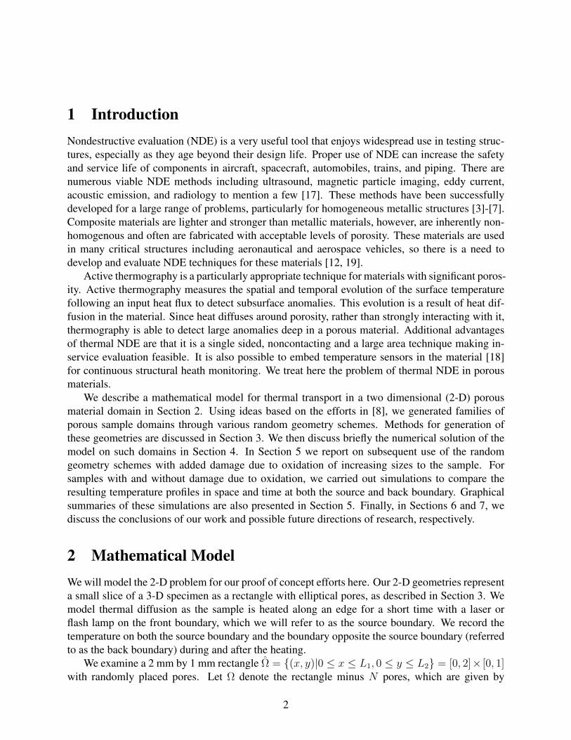
Figure 1: A typical example of a 2-D specimen

Ω1, Ω2, . . . ΩN . The domain of interest is then Ω = Ω ∪ (∪Ni=1Ωi). The exterior boundary of Ω has

4 edges, which we denote by ωj where j=1, . . . , 4; thus ∂Ω = ∪4j=1ωj . It is assumed that each pore

Ωi has a smooth boundary with Ω given by ∂Ωi, as depicted in Figure 1.The 2-D heat diffusion equation, which describes heat as it diffuses through a region, is based

on Fourier’s law and is given [10, 13] by

ρ(x, y)cp(x, y)∂u(t, x, y)

∂t= ∇ · (k(x, y)∇u(t, x, y)). (1)

Here u(t, x, y) is the temperature, ρ(x, y) is the material density of the sample, cp(x, y) is the spe-cific heat of the material, and k(x, y) is the thermal conductivity. We observe that the coefficientsare functions in space which have jump discontinuities at ∂Ωi for i = 1, 2, . . . N . Thus k(x, y) isnot differentiable and therefore in general solutions u(t, x, y) are not twice differentiable in space.Hence the above formulation is clearly inadequate for our problems. We use a variational or weakformulation to avoid these concerns [7].

Let kp denote the thermal conductivity of the pores and km denote that of the material. Thus,the rectangular sample has thermal conductivity

k(x, y) =

kp, (x, y) ∈ Ωi, i = 1, . . . N,

km, (x, y) ∈ Ω.(2)

Consider test functions φ ∈ H1(Ω), in an integrated form of (1) given by∫Ω

cp(x, y)ρ(x, y)∂u

∂tφ(x, y)dA =

∫Ω

φ(x, y)∇ · (k(x, y)∇u)dA. (3)

We rewrite this integral form by decomposing the domain Ω into Ω and Ω1, Ω2, . . . ΩN . Note that

3

k is constant in each subregion. We find∫Ω


∂tφ(x, y)dA

= km

∫Ω

φ(x, y)∇ · (∇u)dA + kp

N∑i=1

∫Ωi

φ(x, y)∇ · (∇u)dA.

(4)

We use Green’s first identity to obtain∫Ω


∂tφ(x, y)dA

=4∑

j=1

(km

∫ωj

φ(x, y)(∇u · nj)ds

)− km

∫Ω

∇u · ∇(φ(x, y))dA

+kp

N∑i=1

(∫∂Ωi

φ(x, y)(∇u · ni)ds−∫

Ωi

∇u · ∇(φ(x, y))dA

).

(5)

The terms∑N

i=1 kp

∫∂Ωi

φ(x, y)(∇u · ni)ds pose a problem because this integration requiresknowledge of the locations of the pores; this is in general unknown. However, if one assumesnegligible heat flux on the boundaries between material and air (a physically reasonable assumptionfor most applications), then ∇u ≈ 0 on ∂Ωi and hence

∑i kp

∫∂Ωi

φ(x, y)(∇u · ni)ds = 0.Combining the three remaining terms from (5), we find∫

Ω


∂tφ(x, y)dA

=4∑

j=1

(km

∫ωj

φ(x, y)(∇u · nj)ds

)−∫

Ω

k(x, y)∇u · ∇φ(x, y)dA.(6)

Excluding the source boundary, we assume an insulated rectangle so that ∇u = 0 on theboundaries ω1, ω2, and ω3. The ω4 or source boundary, which consists of the region (x, 0)|0 ≤x ≤ L1, acts as a source for an initial period and is subsequentially insulated. We represent thecorresponding boundary condition with the characteristic function

km∇u∣∣∣ω4

= S0χ[t0,ts](t) =

S0, t ∈ [t0, ts]

0, otherwise.(7)

Thus we have ∫Ω

cpρ∂u

∂tφ dA =

∫ L1

0

φ(x, 0)S0χ[t0,ts](t) dx−∫

Ω

k∇u · ∇φ dA. (8)

This weak formulation is employed in the MATLAB Partial Differential Equation Toolbox 1 (PDEtoolbox) to provide numerical solutions to the system; this will be discussed further in Section 4.

4

3 Generation of Random GeometriesA major component of the effort reported on here involves generation of domains with randomlyplaced pores of different sizes as depicted in Figure 1 and Figures 3-12. We concentrated ourefforts on elliptical shaped pores with semi-major axes in the horizontal (x) direction. This wasmotivated by visual inspection of material samples at NASA as depicted in Figure 2.

Figure 2: An example of a porous specimen.

We model porosity by randomly placing pores in an L1 = 2 mm by L2 = 1 mm rectangleΩ = [0, 2] × [0, 1] employing ideas developed in [8]. The pores are ellipses to represent voids ina two-dimensional slice of any piece of porous material. For simplicity in algorithm development,we began carrying out our simulations with circles (see [9] for discussions) but subsequently usedellipses for more realistic representations. Even though pores coalesce when they intersect physi-cally, we assume that the pores do not overlap with each other or the boundaries of the rectangularcompartment (more irregular shapes in pores could be achieved by allowing overlaps). To do this,in our algorithms we first generate a pore using one of the probability schemes described below.The pore is then placed in the compartment if it does not overlap with an existing pore, and re-jected if it does. Another pore is then randomly selected as described below, etc., until the desiredporosity of the material is achieved.

3.1 Ellipses: Uniformly Distributed Centers, Bi-Normally Distributed Semi-Axes

We used several probability schemes to generate random ellipses in the compartment Ω. Thepercent porosity, or percent surface area covered by the pores, is an input for each algorithm. Weconsidered pores described by ellipses centered at (x, y) having semi-major axis a and semi-minoraxis b and hence represented by (x− x

a

)2

+(y − y

b

)2

= 1 (9)

5

. The algorithm that we illustrate here created ellipses using a uniform distribution for both the xand y coordinates of the centers and a bi-normal distribution for the semi-major and semi-minoraxes a, b. In this algorithm, we also permitted two sizes of ellipses using a discrete binomialdistribution selecting between smaller ellipses (with a probability of .89) and larger ellipses (witha probability of .11).

3.2 OxidationTo simulate pore-like damages due to oxidation, we first generate one unusually large ellipse (seeSection 5 for examples) to represent damage and then placed pores using the distributions describedabove. When generating various elliptical damages, the center was an input. The semi-major axisfor damage was taken as an input, and the semi-minor axis was calculated so as to maintain aconstant ratio between the two axes as we chose damages of different sizes.

4 Numerical SolutionsAfter generating a particular geometry, we solved the heat equation (8) using PDE Toolbox withthe parameters summarized in Table 1.

Heat transfer coefficient S0 3.3× 104 ergmm2

Material thermal conductivity km 35000 ergmmK sec

Heat capacity cp 7.5× 106 ergg K

Density ρ 1.6× 10−3 gmm3

Table 1: Parameter values

As already noted, three of the compartment’s four sides are insulated and defined by Neumannboundary conditions where heat flux is zero. The source boundary has a heat transfer coefficientof 3.3 × 104 erg/mm2 during flash heating and zero flux later. There is also zero heat flux on theboundaries between the material and the pores; we took pore conductivity kp = 0. PDE Toolboxcreates a mesh using the Delaunay triangulation algorithm and reduces the parabolic equation intoelliptic equations which are solved with the Finite Element Method; see [14] for details. The reduc-tion to elliptic equations assumes time-independence of the boundary conditions; however, recallwe have a time-dependent source boundary. We avoid the associated computational difficulties bysolving the PDE on the interval [t0, ts] and then on t ≥ ts, observing that the boundary conditionsare time-independent on these intervals. The final time for the first solution is ts, which is the initialtime for the second solution and u(ts, x, y) is used as the initial condition for the second solutionto guarantee continuity in time. These two solutions are combined to provide a solution over theentire time interval of interest.

6

We validated the convergence of PDE Toolbox’s numerical solution as outlined in [9] to achieveprecision adequate for our investigations (e.g., 0.04 K for 2% porosity samples and approximately0.1 K for samples with 5% and 10% porosity).

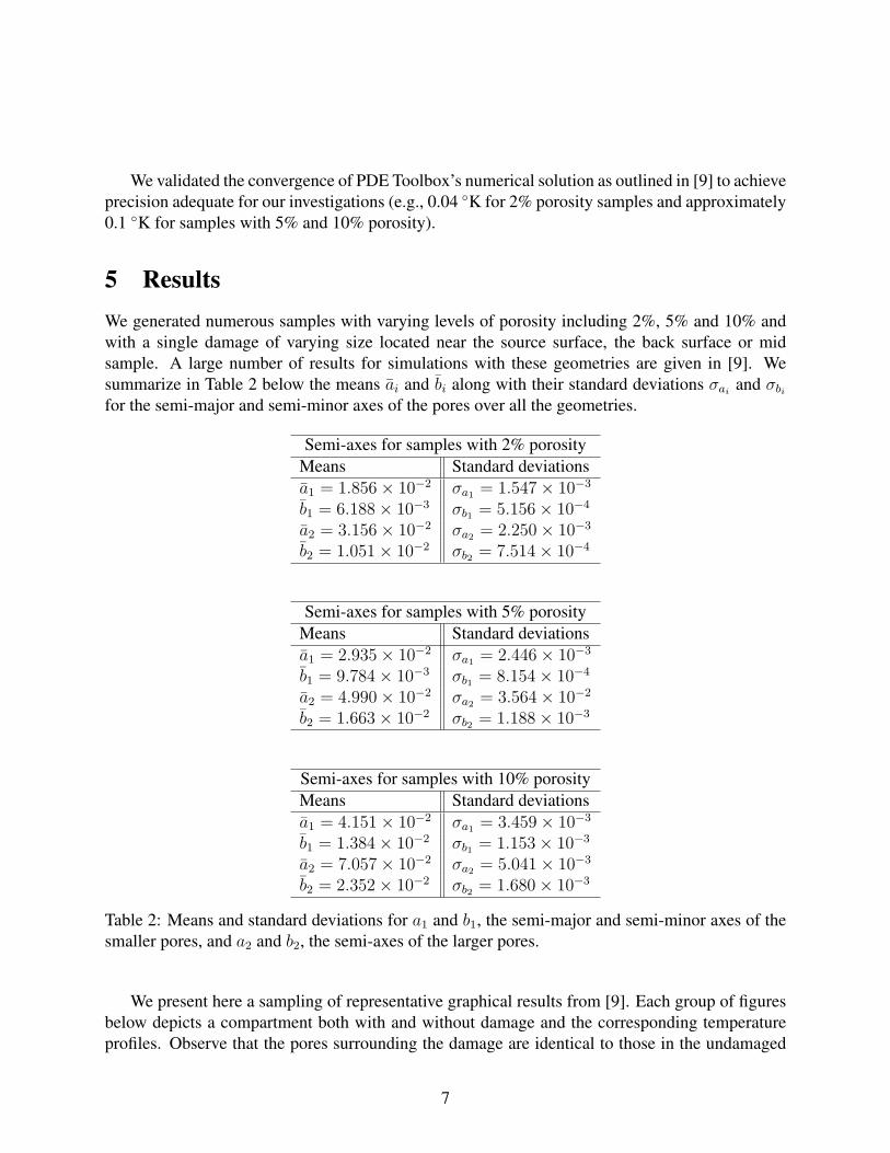
5 ResultsWe generated numerous samples with varying levels of porosity including 2%, 5% and 10% andwith a single damage of varying size located near the source surface, the back surface or midsample. A large number of results for simulations with these geometries are given in [9]. Wesummarize in Table 2 below the means ai and bi along with their standard deviations σai

and σbi

for the semi-major and semi-minor axes of the pores over all the geometries.

Semi-axes for samples with 2% porosityMeans Standard deviationsa1 = 1.856× 10−2 σa1 = 1.547× 10−3

b1 = 6.188× 10−3 σb1 = 5.156× 10−4

a2 = 3.156× 10−2 σa2 = 2.250× 10−3

b2 = 1.051× 10−2 σb2 = 7.514× 10−4


b1 = 9.784× 10−3 σb1 = 8.154× 10−4

a2 = 4.990× 10−2 σa2 = 3.564× 10−2

b2 = 1.663× 10−2 σb2 = 1.188× 10−3


b1 = 1.384× 10−2 σb1 = 1.153× 10−3

a2 = 7.057× 10−2 σa2 = 5.041× 10−3

b2 = 2.352× 10−2 σb2 = 1.680× 10−3

Table 2: Means and standard deviations for a1 and b1, the semi-major and semi-minor axes of thesmaller pores, and a2 and b2, the semi-axes of the larger pores.

We present here a sampling of representative graphical results from [9]. Each group of figuresbelow depicts a compartment both with and without damage and the corresponding temperatureprofiles. Observe that the pores surrounding the damage are identical to those in the undamaged

7

compartment. In every case, we heat the source boundary for 0.6 seconds and record the tempera-ture a total of 1.3 seconds (including heating time). Figures 3-7 and Figures 11-12 present resultsfor samples of varying percent porosity with damages of various size located near the source sur-face. Figure 8 depicts results for mid sample damage while Figures 9 and 10 give results forsamples with damage near the back boundary.

8

0 0.5 1 1.5 20

0.2

0.4

0.6

0.8

1Undamaged Compartment with 2% Porosity

0 0.5 1 1.5 20

0.2

0.4

0.6

0.8

1Damaged Compartment with 2% Porosity

0 0.2 0.4 0.6 0.8 1 1.2 1.4 1.6 1.8 20.06

0.08

0.1

0.12

0.14

0.16

0.18

0.2

0.22

0.24

0.26Temperature Difference Between Source and Back

Position Along x−axis (mm)

Tem

pera

ture

(K)

UndamagedDamaged

0 0.2 0.4 0.6 0.8 1 1.2 1.4 1.6 1.8 2−0.02

0

0.02

0.04

0.06

0.08

0.1

0.12

0.14

0.16

0.18Difference Between Temperature With and Without Damage


Tem

pera

ture

(K)

Source BoundaryBack Boundary

Figure 3: Sample with 2% porosity, damage centered at (1, 0.2), semi-major axis a = 0.35 mm,semi-minor axis b = 0.0346 mm.

0 0.5 1 1.5 20

0.2

0.4

0.6

0.8


0 0.5 1 1.5 20

0.2

0.4

0.6

0.8


0 0.2 0.4 0.6 0.8 1 1.2 1.4 1.6 1.8 20

0.2

0.4

0.6

0.8

1

1.2



Tem

pera

ture

(K)

UndamagedDamaged

0 0.2 0.4 0.6 0.8 1 1.2 1.4 1.6 1.8 2−0.2

0

0.2

0.4

0.6

0.8

1

1.2



Tem

pera

ture

(K)



9

0 0.5 1 1.5 20

0.2

0.4

0.6

0.8


0 0.5 1 1.5 20

0.2

0.4

0.6

0.8


0 0.2 0.4 0.6 0.8 1 1.2 1.4 1.6 1.8 20.1

0.15

0.2

0.25

0.3



Tem

pera

ture

(K)

UndamagedDamaged

0 0.2 0.4 0.6 0.8 1 1.2 1.4 1.6 1.8 2−0.05

0

0.05

0.1

0.15



Tem

pera

ture

(K)



0 0.5 1 1.5 20

0.2

0.4

0.6

0.8


0 0.5 1 1.5 20

0.2

0.4

0.6

0.8


0 0.2 0.4 0.6 0.8 1 1.2 1.4 1.6 1.8 20

0.1

0.2

0.3

0.4

0.5

0.6



Tem

pera

ture

(K)

UndamagedDamaged

0 0.2 0.4 0.6 0.8 1 1.2 1.4 1.6 1.8 2−0.1

0

0.1

0.2

0.3

0.4

0.5



Tem

pera

ture

(K)



10

0 0.5 1 1.5 20

0.2

0.4

0.6

0.8


0 0.5 1 1.5 20

0.2

0.4

0.6

0.8


0 0.2 0.4 0.6 0.8 1 1.2 1.4 1.6 1.8 20

0.5

1



Tem

pera

ture

(K)

UndamagedDamaged

0 0.2 0.4 0.6 0.8 1 1.2 1.4 1.6 1.8 2−0.2

0

0.2

0.4

0.6

0.8

1

1.2


Position Along x−axis (mm)Te

mpe

ratu

re (K

)



0 0.5 1 1.5 20

0.2

0.4

0.6

0.8


0 0.5 1 1.5 20

0.2

0.4

0.6

0.8


0 0.2 0.4 0.6 0.8 1 1.2 1.4 1.6 1.8 20.05

0.1

0.15

0.2

0.25

0.3

0.35

0.4



Tem

pera

ture

(K)

UndamagedDamaged

0 0.2 0.4 0.6 0.8 1 1.2 1.4 1.6 1.8 2−0.1

−0.05

0

0.05

0.1

0.15

0.2

0.25



Tem

pera

ture

(K)



11

0 0.5 1 1.5 20

0.2

0.4

0.6

0.8


0 0.5 1 1.5 20

0.2

0.4

0.6

0.8


0 0.2 0.4 0.6 0.8 1 1.2 1.4 1.6 1.8 2

0.1

0.15

0.2

0.25

Temperature Difference Between Source and Back


Tem

pera

ture

(K)

UndamagedDamaged

0 0.2 0.4 0.6 0.8 1 1.2 1.4 1.6 1.8 2

−0.05

0

0.05

0.1

Difference Between Temperature With and Without Damage


Tem

pera

ture

(K)



0 0.5 1 1.5 20

0.2

0.4

0.6

0.8


0 0.5 1 1.5 20

0.2

0.4

0.6

0.8


0 0.2 0.4 0.6 0.8 1 1.2 1.4 1.6 1.8 20.05

0.1

0.15

0.2

0.25

0.3

0.35

0.4



Tem

pera

ture

(K)

UndamagedDamaged

0 0.2 0.4 0.6 0.8 1 1.2 1.4 1.6 1.8 2−0.15

−0.1

−0.05

0

0.05

0.1

0.15



Tem

pera

ture

(K)



12

0 0.5 1 1.5 20

0.2

0.4

0.6

0.8


0 0.5 1 1.5 20

0.2

0.4

0.6

0.8


0 0.2 0.4 0.6 0.8 1 1.2 1.4 1.6 1.8 20.1

0.15

0.2

0.25

0.3

0.35

0.4



Tem

pera

ture

(K)

UndamagedDamaged

0 0.2 0.4 0.6 0.8 1 1.2 1.4 1.6 1.8 2−0.05

0

0.05

0.1

0.15

0.2

0.25



Tem

pera

ture

(K)



0 0.5 1 1.5 20

0.2

0.4

0.6

0.8


0 0.5 1 1.5 20

0.2

0.4

0.6

0.8


0 0.2 0.4 0.6 0.8 1 1.2 1.4 1.6 1.8 20

0.2

0.4

0.6

0.8

1

1.2

1.4

1.6



Tem

pera

ture

(K)

UndamagedDamaged

0 0.2 0.4 0.6 0.8 1 1.2 1.4 1.6 1.8 2−0.2

0

0.2

0.4

0.6

0.8

1

1.2



Tem

pera

ture

(K)



13

6 Discussion and ConclusionsWe observed several general trends in our temperature profile graphs. First, we tracked tempera-tures at the source and back boundaries so as to shed light on possible sensor placement if optionswere available. As might be expected, we found that the absolute value of the difference betweendamaged and undamaged material is greatest at the center of the damage due to oxidation. At 2%porosity with a damage due to oxidation width of 0.7 mm near the source boundary, the maximumdifference between the damaged and undamaged material is approximately 0.18 K at the sourceboundary and 0.02 K at the back boundary; this is depicted in Figure 3. As shown in Figure 4,at a damage width of 1.4 mm due to oxidation, the maximum difference is 1.2 K at the sourceboundary and 0.03 K at the back boundary. In Figure 5, we see that at 5% porosity, the maximumdifference between undamaged and damaged material at the source boundary is 0.2 K while atthe back boundary the maximum difference is 0.02 K for a damage width of 0.7 mm. In Figure 7,when the damage width increases to 1.4 mm, the maximum difference is 1.35 K at the sourceboundary and 0.08 K at the back boundary. At 10% porosity, the maximum difference is 0.24K at the source boundary and 0.02 K at the back boundary for a damage width of 0.7 mm, asseen in Figure 11. When the size of the damage is increased to a width of 1.4 mm, we find inFigure 12 that maximum temperature difference is 1.4 K at the source boundary and 0.09 K atthe back boundary. These observations demonstrate that the maximum temperature difference be-tween damaged and undamaged material at the source boundary is larger than at the back boundarywhen the damage is placed near the source boundary. We anticipate that with a sensor that has 0.1K resolution, placed on the source boundary, we will be able to detect 0.7 and 1.4 mm damagesdue to oxidation in materials with 2, 5, or 10% porosity. With the same sensor placed on the backboundary, we would not expect to be able to detect these damages in any of the materials.

The difference between damaged and undamaged material is greatest at the center of the dam-age due to oxidation for both the source and back boundary measurements in most of our computa-tions. The source boundary temperature is always higher with damage, whereas the back boundarytemperature is lower with damage in most of our computations. When the damage is placed nearthe source boundary, the absolute value of the temperature difference resulting from the damageis much greater for the source boundary than the back boundary. When the damage is placed atthe center of the compartment, the absolute value of the temperature difference is approximatelythe same for the source and back boundaries. And lastly, when the damage is placed near the backboundary, the absolute value of the the temperature difference is much greater for the back bound-ary than the source boundary. At 5% porosity, for example, a 1.05 mm wide damage placed nearthe source boundary results in a 0.57 K change in temperature at the source boundary and a 0.02K change in temperature at the back boundary; this is depicted in Figure 6. When the same sizeddamage is placed in the middle of the compartment, one can see a 0.25 K change in temperatureat the source boundary and a 0.11 K change in temperature at the back boundary, as shown inFigure 8. When the damage is placed near the back boundary, one can see a 0.1 K change intemperature at the source boundary and a 0.08 K change in temperature at the back boundary(note that the magnitude of the temperature change decreases as the damage moves away from thesource boundary); see Figure 9. These observations are important because they help to better iden-

14

tify the location of the damage. In Figure 5, for example, at 5% porosity, a damage of width 0.7mm centered near the source boundary results in a temperature difference of 0.19 K at the sourceboundary. Meanwhile, in Figure 10, at the same porosity, a damage of width 1.4 mm near the backboundary gives an equal temperature difference. When we consider the change in temperature(the maximum difference minus the minimum difference), however, we are able to determine thelocation of the damage. When the damage is centered near the back, the change in temperature is0.22 K for the back boundary and only 0.03 K for the source boundary. As depicted in Figure 7,when the damage is centered near the source, the change in temperature at the source is 0.89 K,and 0.11 K for the back boundary. Thus, by comparing sensors at the back surface with those atthe source surface, one should be able to discern the depth of the damage if it is of sufficient size.

We also observed two general trends in the temperature vs. time graphs (in results given in [9]but not depicted here). As the size of the damage due to oxidation grows, it takes longer for thesystem to reach thermal equilibrium. The farther away the damage is from the source boundary,the closer together the source and back boundary temperatures are for both x = 1 and x = 0.

7 Further WorkThe results developed here not only provide useful information regarding the detection of damagedue to oxidation, but also provide methods of generating synthetic data that may be used for furtheranalysis as well. We would like to develop a method of separating the effect of porosity (whichmight reasonably be viewed as random noise) from the effect of damage in effective thermal dif-fusivity. In order to do this, we must develop parameter estimation techniques. There are variousmethods which use flash heating to estimate the effective thermal diffusivity; some of these meth-ods are discussed in [10] and [15]. We also plan on investigating homogenization and the limitsof its usefulness in detecting damages in porous materials. Homogenization theory assumes peri-odicity in the coefficients of the partial differential equation. The usual theory [11] requires thatperiodicity go to zero in some sense. The periodicity of the coefficients is a result of periodic ge-ometry (for instance we could have a geometry with an infinite number of infinitely small circleswithin a rectangle) though homogenization can be applied to more complex geometries [1, 2]. Ifthere are not many pores or the pores are too large, we expect homogenization will not provide agood approximation, while if we have a high number of small pores, we suspect homogenizationwill be a good approximation. There are many advantages to using homogenization theory. After alimit is taken, we are left with a constant coefficient partial differential equation on a homogeneoussquare, which is readily treated numerically. Also, homogenization can be used in n dimensions.Damage here is neither “small” nor “periodic”, so homogenization cannot be used to study thisaspect of our problem. We hope to use homogenization theory both in a local or regional sense(i.e., near surface vs. deep interrogations) to determine the effects of the porosity in the early timebehavior of the thermal diffusivity and then remove this effect from later time behavior to gain aresolved effect of the damage as reflected in the thermal diffusivity or conductivity [16]. Of course,to be useful as a basis for a widely applicable interrogation technology, these investigations musteventually be carried out for three dimensional geometries with random porosities.

15

8 AcknowledgmentsThis research, which was begun as part of an REU project at North Carolina State University forco-authors BB, KF, CU, and TV, which was supported in part by the National Science Founda-tion (NSF) under grant DMS-0552571, and in part by the National Security Agency under grantH98230-08-1-0094. It was also supported in part (AKC) by the National Science Foundation(NSF) under grant DMS-0636590, and in part (HTB and AKC) by NASA under grant NIA/NCSU-03-01-2536-NC.

References[1] E. Acerbi, V. C. Piat, G. D. Maso, and D. Percivale, An extension theorem from connected

sets, and homogenization in general periodic domains, Nonlinear Analysis: Theory, methodsand applications, 18 (1992), 481–496.

[2] N. S. Bakhvalov and J. S. J. Paulin, Homogenization for thermoconductivity in a porousmedium with periods of different orders in the different directions, Asymptotic Analysis, 13(1996), 253–276.

[3] H. T. Banks, N. L. Gibson, and W. P. Winfree, Void detection in complex geometries, Centerfor Research in Scientific Computation Technical Report, CRSC-TR08-09, NCSU, May,2008.

[4] H. T. Banks, M. L. Joyner, B. Wincheski, and W. P. Winfree, Nondestructive evaluationusing a reduced-order computational methodology, Inverse Problems, 16 (2000), 929–945.

[5] H.T. Banks and F. Kojima, Boundary shape identification problems in two-dimensional do-mains related to thermal testing of materials, Quarterly of Applied Mathematics, 47 (1989),273–293.

[6] H. T. Banks and F. Kojima, Identification of material damage in two-dimenstional domainsusing the SQID-based nondestructive evaluation system, Inverse Problems, 18 (2002), 1831-1855.

[7] H. T. Banks, F. Kojima, and W. P. Winfree, Boundary estimation problems arising in thermaltomography, Inverse Problems, 6 (1990), 897–921.

[8] K. L. Bihari, Analysis of Thermal Conductivity in Composite Adhesives, PhD thesis, NorthCarolina State University, Raleigh, 2001.

[9] B. Boudreaux, K. Foster, C. Uttal, T. Vogel, H.T. Banks, A.K. Criner, and W.P. Winfree,Thermal Interrogation of Porous Materials, Center for Research in Scientific ComputationTechnical Report CRSC-TR08-11, North Carolina State University, Raleigh, September,2008.

16

[10] H. S. Carslaw and J. C. Jaeger, Conduction of Heat in Solids, Oxford University Press, 1959.

[11] D. Cioranescu and P. Donato, An Introduction to Homogenization, Oxford University Press,1999.

[12] K. E. Cramer, W. P. Winfree, K. Hodges, A. Koshti, D. Ryan, and W. W. Reinhardt, Status ofthermal NDT of space shuttle materials at NASA, in 9th Joint FAA/DoD/NASA Conferenceon Aging Aircraft, 2007.

[13] F. Incropera and D. Dewitt, Fundamentals of Heat and Mass Transfer, John Wiley & Sons,New York, 1990.

[14] The Mathworks, Inc., Partial Differential Equation Toolbox 1: User’s Guide, 2008.

[15] W. J. Parker, R. J. Jenkings, C. P. Butler, and G. L. Abbott, Flash method of determiningthermal diffusivity, heat capacity, and thermal conductivity, Journal of Applied Physics, 32(1961), 1679–1684.

[16] S Schmauder and U. Weber, Modelling of functionally graded materials by numerical ho-mogenization, Archive of Applied Mechanics, 71 (2001), 182–192.

[17] P. J. Shull (ed.), Nondestructive Evaluation: Theory, Techniques, and Applications, MarcelDekker, Inc., 2001.

[18] A. Stewart, G. Carman, and L. Richards, Nondestructive evaluation technique utilizing em-bedded thermal fiber optic sensors, Journal of Composite Materials, 37 (2003), 2197–2206.

[19] W. P. Winfree, E. I. Madaras, K. E. Cramer, P. A. Howell, K. L. Hodges, J. P. Seebo, andJ. L. Grainger, NASA Langley inspection of rudder and composite tail of American Air-lines flight 587, in 46th AIAA/ASME/ASCE/AHS/ASC Structures, Structural Dynamics andMaterials Conference, 2005.

17

Documents

Thermal Based Damage Detection in Porous Materials · PDF fileThermal Based Damage Detection in Porous Materials ... the use of the heat equation to simulate a thermal ... the MATLAB