Thermal Energy Storage for the NIST Net-Zero House Heat …

i

NIST Technical Note 2005

Thermal Energy Storage for the NIST

Net-Zero House Heat Pump

M. A. Kedzierski

W. V. Payne

H. M. Skye

https://doi.org/10.6028/NIST.TN.2005

ii

NIST Technical Note 2005

Thermal Energy Storage for the NIST

Net-Zero House Heat Pump

M. A. Kedzierski

W. V. Payne

H. M. Skye

Energy and Environment Division

Engineering Laboratory

This publication is available free of charge from:

https://doi.org/10.6028/NIST.TN.2005

July 2018

U.S. Department of Commerce Wilbur L. Ross Jr., Secretary

National Institute of Standards and Technology

Walter Copan, NIST Director and Undersecretary of Commerce for Standards and Technology

iii

Certain commercial entities, equipment, or materials may be identified in this

document in order to describe an experimental procedure or concept adequately.

Such identification is not intended to imply recommendation or endorsement by the

National Institute of Standards and Technology, nor is it intended to imply that the

entities, materials, or equipment are necessarily the best available for the purpose.

National Institute of Standards and Technology Technical Note 2005

Natl. Inst. Stand. Technol. Tech. Note 2005, 31 pages (July 2018)

CODEN: NTNOEF

This publication is available free of charge from: https://doi.org/10.6028/NIST.TN.2005

1

Thermal Energy Storage for the NIST Net-Zero House Heat Pump

Mark. A. Kedzierski1

W. Vance. Payne

Harrison. M. Skye

National Institute of Standards and Technology

Gaithersburg, MD 20899

ABSTRACT

This report investigates the viability of thermal energy storage by using a phase-change material

(PCM) for residential air-conditioning. The air-conditioning performance and the associated

external and internal heat loads to the National Institute of Standards and Technology’s Net-Zero

Energy Residential Test Facility (NZERTF) were modelled for a single day near the summer

solstice. The transient model predicted the frequency and the duration of the cooling cycles for

the air-source heat pump with and without PCM. The model was used to examine two different

PCM energy storage configurations for their efficacy in improving energy efficiency and/or in

meeting the entire peak cooling load for the house. The first configuration limited the mass of the

PCM to minimize the required changes to a conventional cooling system. The main component

of the first type of cooling system was the integrated PCM evaporator, where a limited amount of

PCM was made an integral part of the evaporator and placed within an annulus that surrounded

the refrigerant tube. The system with the integral PCM evaporator showed no potential advantage

over a conventional system with a larger evaporator and a smaller compressor. The system with

the integral PCM evaporator also failed to deliver improved energy savings and peak load shifting

due to insufficient amount of PCM and a significant resistance to heat transfer through the PCM

within the annulus. In contrast, the second configuration for the residential cooling system, which

used remotely stored PCM, exhibited significant energy savings while shifting the entire peak

thermal building load to the PCM energy storage with minimal electricity used during the peak

load. The remote PCM system achieved between a 6 % and a 33 % reduction in the required

electrical energy for the entire cooling day, depending on the PCM thermal resistance, while

maintaining acceptable indoor humidity ratios. The performance was best when the heat transfer

resistance between the PCM and the evaporating refrigerant was minimized.

Keywords: air conditioning, energy storage, residential

1 Corresponding author. Tel./fax: (301) 975-5282/(301) 975-8973. E-mail address: [email protected]

2

TABLE OF CONTENTS

ABSTRACT ............................................................................................................................. 1 TABLE OF CONTENTS ....................................................................................................... 2

LIST OF FIGURES ................................................................................................................ 2 INTRODUCTION................................................................................................................... 3 MODELING BASE CASE ..................................................................................................... 4 MODELING WITH PCM ENERGY STORAGE ............................................................. 10 CONCLUSIONS ................................................................................................................... 18

ACKNOWLEDGEMENTS ................................................................................................. 18 NOMENCLATURE .............................................................................................................. 19

LIST OF FIGURES

Figure 1 Outdoor temperature for June 17, 2017 ............................................................. 20

Figure 2 Energy balance for NZERTF .............................................................................. 20 Figure 3 Humidity ratio for the NZERTF on June 17, 2017 ........................................... 20

Figure 4 Plug loads for NZERTF on June 17, 2017 .......................................................... 20 Figure 5 Solar heat gain on June 17, 2017 ......................................................................... 20 Figure 6 NZERTF air-source heat pump schematic (Davis et al., 2014) ........................ 20

Figure 7 COP for 20th cycle on June 17, 2017 ................................................................... 20 Figure 8 Comparison of measured COP to that predicted with eq. (3) for all 37

cycles........................................................................................................................... 20 Figure 9 Comparison of measured compressor and fan work to that predicted with

eq. (11) for all 37 cycles............................................................................................. 20

Figure 10 Comparison of measured compressor and fan work that predicted with

eq. (11) for 20th cycle on June 17, 2017 .................................................................. 20 Figure 11 Comparison of measured evaporator capacity to that predicted with

eq. (12) for 20th cycle on June 17, 2017 ................................................................... 20

Figure 12 Measured evaporator capacity for all cycles of June 17, 2017 ....................... 20 Figure 13 Predicted evaporator capacity for all cycles of June 17, 2017 ........................ 20

Figure 14 Comparison of measured to predicted compressor run time for all cycle of

June 17, 2017 ............................................................................................................. 20 Figure 15 Proposed PCM evaporator for investigation (Kedzierski et al., 2014) .......... 20 Figure 16 Shamsundar and Sparrow (1974) model for freezing and melting time for

PCM ........................................................................................................................... 20

Figure 17 Indoor air temperature when using integrated PCM evaporator and 1 ton

two-speed compressor ............................................................................................... 20

Figure 18 Indoor humidity ratio when using integrated PCM evaporator and 1 ton,

two-speed compressor ............................................................................................... 20 Figure 19 Schematic of remote PCM storage for residential air conditioning .............. 20 Figure 20 Effect of heat transfer resistance on required compressor and outdoor fan

work for remote storage ........................................................................................... 20 Figure 21 Effect of heat transfer resistance on indoor humidity ratio when using

remote PCM and 1 ton compressor ......................................................................... 20

3

INTRODUCTION

Using water as a phase-change material (PCM) is a popular way to provide air conditioning for

large buildings. One benefit is that ice is made during the night when commercial electricity rates

are significantly lower than during the day when the demand for electricity is high. In addition,

chillers for making ice can be smaller than those sized to meet the building’s immediate cooling

demand because the smaller chillers can operate continuously throughout the night to make enough

ice for the next day’s peak use (ASHRAE, 2015). Residential electricity rates typically do not

vary with the time of day, so making ice during the night has limited application for homes.

However, ice storage can provide an alternative to exporting excess renewable electricity to the

grid. As an example, the electricity produced by a wind turbine during the night could be used to

power an ice-making machine for thermal storage. Ice made at night would be done at greater or

comparable system efficiency due to lower outdoor air/condensing temperatures as compared to

those during the day (ASHRAE, 2015). A home might have two separate systems for cooling: a

relatively small chiller for making ice and a heat pump to meet the cooling demands when there is

no stored ice. Work toward the realization of residential ice storage would benefit from ice heat

transfer research. Pumping ice/water mixtures (ice slurries) or ice forming on coils are two

potential research areas. Ice slurry and melt-ice-on-coil heat transfer studies like those done by

Kumano et al. (2014) and Lo´pez-Navarro et al. (2013), respectively, would have to be either

adapted or re-done for residential applications.

Measurements at the National Institute of Standards and Technology (NIST) net-zero energy

residential test facility (NZERTF)2 shows that the air-source heat pump (ASHP) consumes

approximately 45 % - the largest share - of the home’s total energy. Reducing this energy

consumption is difficult because the efficiency of conventional ASHPs is nearing its practical limit

due to intrinsic irreversibilities that cannot be mitigated. Nevertheless, energy savings remain

achievable by increasing the cycle Coefficient of Performance (COP). One characteristic of the

COP is that it decreases as the “lift,” i.e., the difference between the indoor and outdoor air

temperatures with which the ASHP work, increases. The lift is directly proportional to the space

conditioning need, causing the heat pump to operate at a lower efficiency during the time when

the building thermal load is greatest. These two factors are the major contributing causes of the

electricity usage peak experienced by electrical utilities during the summer months. Air

conditioning using thermal storage would contribute to the stability and reliability of utility power

generation during the peak hours. Consequently, a non-conventional ASHP that enables

residential load shifting and exceeds the current state-of-the-art COPs would be required to support

to grid reliability.

A non-conventional, highly efficient, ASHP can be realized by using PCM-based Thermal Energy

Storage (TES) during off peak times (Kedzierski, et al., 2014). In addition to increased efficiency,

the PCM can be used for load shifting. Kedzierski et al. (2014) suggested that the key to realizing

the efficiency improvements is to use PCM in conjunction with a compressor that is approximately

half the size of a conventional system to meet a particular space-conditioning load. That report

noted that the required size of the compressor would be reduced because the peak load would be

met by the combined capacity of the mechanical air-conditioning and the melting of the PCM. It

was further suggested that the daily efficiency would be improved because the unit runs nearly

2 Referred to as the “house” for brevity and clarity in much of this manuscript.

4

continuously instead of cycling on and off to meet the load, thus, avoiding a typical 2 % to 8 %

loss in efficiency due to cycling (Baxter and Moyers 1985). Further efficiency improvements

would be achieved because the PCM is recharged when the lift and the space-conditioning loads

are the smallest. It was also proposed to use the stored energy to provide space conditioning during

high lift conditions.

Kedzierski et al. (2014) identified three different conceptual designs for PCM storage with a

residential (ASHP). The first design, “integrated PCM”, directly coupled the PCM with the indoor

tube-fin heat exchanger. This design benefits from simplicity, but it was expected to be somewhat

limited by the amount of PCM that can be included within the heat exchanger volume and

footprint. The second and the third designs used a “discrete PCM” configuration, which locates

the PCM remotely in a storage tank. The second design used the ASHP working fluid (i.e.

refrigerant) to deliver/remove energy to/from the remotely located PCM. The third design pumped

the remotely stored PCM to a heat exchanger in the air handler. The drawbacks of the second and

the third designs include increased complexity and additional components, which increase the cost

and parasitic losses.

Models for the integrated and the discrete PCM configurations do not exist in the literature. The

purpose of the present investigation is to model both the integrated and discrete PCM energy

storage for use in air conditioning NIST’s NZERTF. Accordingly, this paper determines the

salient design parameters for an efficient and viable thermal energy storage using phase-change

materials in a heat pump for net-zero homes.

MODELING BASE CASE

This section presents the model development and validation for predicting the house heat loads

and the transient cooling performance of the NZERTF for June 17, 2017. The heat transferred

through the house with and without a solar load was modeled along with the performance of the

air-conditioning system. The cooling performance and the incident heat loads were modeled from

existing measurements. The uncertainties for the measurements that were modelled in this study

are taken from Davis et al. (2014) unless otherwise stated. All of the measurement uncertainties

provided here are expanded uncertainties with a 95 % confidence level (i.e., coverage factor of 2).

House Loads for June 17, 2017

A simplified approach was used to model the performance of the NZERTF air-conditioning system

for a single high-load day that occurred near the summer solstice on June 17, 2017. The outdoor

air temperature (T), measured at the air intake for the outdoor condensing unit of the air

conditioner, is shown in Fig. 1 as open circles. T is plotted as a function of the time of day (t)

with a time of zero being midnight on June 16, 2017 and has an uncertainty of ± 0.7 K3. The solid

line in Fig. 1 shows the fit of T with respect to time that was developed for this analysis:

5 14.28[K]sin(7.32 10 [s ]( 37102[s])) 298.72[K]T t (1)

Equation (1) is dimensional, with time having units of seconds and T having units of Kelvin. The

absolute, average difference between eq. (1) and the measured T is approximately ± 1 K. The

3 All temperature measurements provided in this study have an uncertainty of ± 0.7 K and a confidence level of

95 %.

5

form of eq. (1) was chosen solely because of its ability to replicate the measure outdoor

temperature as a function of time.

The thermostat that controlled the on/off operation of the air-conditioning was set to maintain the

indoor air temperature (Tai) of the house at approximately 297 K. As a result of the difference

between Tai and T, heat was transferred between the air inside the house and the outdoor air. This

heat transfer (qUA) was calculated as occurring independent of the solar sun load (qs) of the house

and was primarily governed by the combined conduction resistance through the walls, roof and

windows, while neglecting heat transfer associated with air infiltration. An estimate for the

average overall heat transfer coefficient through the walls, the roof and the windows (UA) can be

written as a surface area weighted summation of the conduction heat transfer coefficients in

parallel:

UA

w w WN WN r r

ai( )T T

qUA h A h A h A

(2)

Here, the average conduction heat-transfer coefficients for the wall, the windows, and the roof (hw,

hWN, and hr, respectively) are taken as the reciprocal of the conductive resistances given in Pettit

et al. (2015). Pettit et al. (2015) provided the composite conductive resistances (R-values) for the

walls, the windows, and the roof as R-45, R-5.2, and R-72, respectively, which corresponds to

heat-transfer coefficients of approximately 0.126 Wm-2K-1, 0.109 Wm-2K-1, and 0.079 Wm-2K-1,

respectively. The NZERTF construction mainly follows the “perfect wall” design concept

(Lstiburek, 2010), which significantly reduces the effect thermal bridging caused by structural

elements. Substitution of these heat transfer coefficients and the surface areas from Pettit et al.

(2015), and provided in Fig. 2, gives the estimated UA from eq. (2) as 90 WK-1.

In contrast, the UA obtained for the house, averaged over an eight-month period for mainly heating

conditions by Omar et al. (2017), was 172 WK-1. The larger UA obtained by Omar et al. (2017)

as compared to the value obtained from the R-values and eq. (2) may be due to the over estimation

of the R-values for the windows in eq. (2) and the lack of inclusion of the heat transfer through the

foundation of the house. These UA values also differ from the UA that was obtained in the present

study for a single cooling day. That UA value of 150 WK-1 was obtained by trial and error such

that the predicted cycles for the cooling heat load matched the duration and frequency of those

measured in the morning hours when the solar load was not present. The difference between this

cooling-estimated UA and that obtained by Omar et al. (2017) is roughly 13 %. Omar et al. (2017)

did show that their UA was within 7 WK-1 of a UA obtained for the same heating measurements

using a different method; however, no measurement uncertainty was provided that could be used

to determine if 7 WK-1 was within the uncertainty. One possible explanation for the difference

between the present UA (150 WK-1) and that obtained by Omar et al. (2017) is that neither method

accounts for the heat recovery ventilator (HRV) which brings in cold outdoor air in the winter and

hot outdoor air in the summer. The Omar et al. (2017) data contained all the winter months where

the average temperature difference between the inside and the outside of the house was

approximately 20 K as compared to an average temperature difference of roughly 2 K for the June

17 data. For the winter heating data, the UA is associated with the loss of heat to the outside. Not

accounting for the HRV caused the UA to effectively increase in order to account for the additional

cooling by the HRV in the winter.

6

Figure 2 illustrates the transient energy balance on the total mass of moist air (Ma) in the house:

a

aiST a s g UA e

d

dp

TE M c q q q q

t (3)

The energy stored in the air (EST) is equal the product of the Ma, the specific heat of the moist air

(cpa) and the rate of change of the indoor air temperature (Tai) with respect to time (t). Here qe is

the cooling heat load for the house air, which is a sum of the sensible (q1) and the latent heat (q2)

loads. The symbol for the plug heat load is qg. The heat transferred by conduction through the

walls, the windows, and the roof (qUA) was calculated from eq. (2) and the temperature difference

between the inside and outside air. The qUA was negative when heat was transferred from the

inside of the house to the outside in the morning hours when the outdoor temperature was less than

the indoor temperature.

Use of eq. (3) implies the assumption that the house air is at uniform air temperature, which is

generally not the case: measured temperature differences between rooms can be as much as 2 K

(Omar, 2017). A model that accounts for the transient nonuniformity of the house air temperature

would be computationally intensive and not expected to yield significantly more accurate results

as compared to the present model that uses the “lumped capacitance” assumption for a uniform

air-temperature distribution. The lumped capacitance assumption is appropriate for the present

analysis because the resistance for heat transfer between the inside air and the outside air is

significantly larger than the heat transfer resistance between the ASHP and the inside air (Incropera

and DeWitt, 2002).

The humidity ratio is defined as the ratio of the mass of water vapor in the air to the mass of indoor

dry air. Figure 3 shows the humidity ratio for the indoor conditioned air, which was calculated

from the measured dew-point temperature of the return air to the evaporator with an uncertainty

of ± 5 %. Direct local measurements of the humidity ratios were made. However, the humidity

ratio obtained from the measured average air properties provided for a more representative average

value than the average of the local humidity measurements. The latent load for the house was

calculated from the derivative of the transient humidity ratio with respect to time (dw/dt), the mass

of dry air in the house, and the latent heat of vaporization of water (ifg) as:

1

a fg d e2

d1592.42 W K 5935.73 W

d

wq M i T T

t

(4)

Using eq. (4), a linear fit of the q2 was done with respect to the difference between the measured

dew-point temperature of the air (Td) and the measured surface temperature of the evaporator

(Te). The uncertainty of the fit shown in eq. (4) was roughly ± 10 % of the predicted value.

Figure 3 shows that the measured humidity ratios were less than 0.012 for more than 80 % of the

day while the setpoint temperature was satisfied, which is consistent with the requirements in

ASHRAE Standard 55 (2017).

7

The plug heat load (qg) for June 17, 2017 is shown in Fig. 4 as a function of time where

instantaneous spike loads were removed, and qg was smoothed so that the total area under the curve

remained approximately the same.

The solar irradiance (Is) incident on the house on June 17, 2017 was measured with a flat-plate

silicon pyranometer located on the ridge of the main roof to an uncertainty of ± 5 %. The solar

heat gain (qs) can be calculated from the Is if the Solar Heat Gain Coefficient (SHGC) and the

effective window area (AWN) are known (Omar et al., 2017):

s s WN SHGC q I A (5)

According to Pettit et al. (2015), the SHGC for the windows of the house is 0.25, and the south

facing window area is approximately 16.5 m2. A first estimate for the product of SHGC·AWN,

assume that window blinds cover half of the windows, would be 2.06 m2. This is close to the final

value that was used (2.64 m2), which was obtained by trial and error to give the best agreement

between the measured and predicted duration, number, and time of the cooling cycles.

The solar heat gain (qs) to the house was modeled during midday for times between 35000 s and

80000 s as:

s

5 12800[W]sin(6.98 10 [s ]( 35000[s]))q t (6)

For times outside of midday, i.e., t < 35000 s and t > 80000 s, qs was set to zero. The peak solar

gain from eq. (6) occurred at t = 57500 s or 15:58:20 Daylight Saving Time (DST) (3:58:20 p.m.),

which lags the peak incident solar radiation to the house as given by Omar (2017) on that day by

approximately 10400 s (2.9 h). Figure 5 compares the qs calculated from eq. (5) using 2.64 m2 for

SHGC·AWN and the measured Is (Omar, 2017) to the qs as predicted from eq. (6).

Air-Source Heat Pump

The instrumentation, data acquisition system, and measurement uncertainty associated with the

R410A air-source heat pump, as well as all other electrical/mechanical systems within the

NZERTF, are described in detail by Davis et al. (2014). Figure 6 shows a schematic of the heat

pump and the location of the instrumentation. When the heat pump is operated in the air-

conditioning mode, the indoor unit contains the evaporator, which is identified as the indoor coil

in Fig. 6. The cooling capacity, qe, is associated with this coil. The indoor unit is also shown to

contain a fan that delivers the air from the house returns to the evaporator for cooling. The outdoor

fan is not shown in Fig. 5.

8

The Wc was the sum of the electrical work of the indoor fan the outdoor unit, which included the

outdoor fan, the compressor, and controls. The Coefficient of Performance (COP) of the air-

conditioning unit was calculated from the measured evaporator heat duty (qe) and the total

electrical work input (Wc) as:

e

c

COPq

W (7)

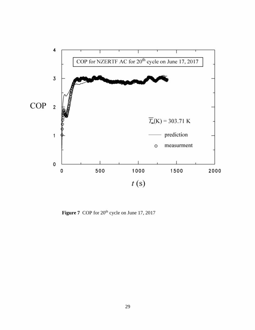
Figure 7 shows the COP for one of the 37 cycles that occurred during the observed day for the

NZERTF ASHP. The time was set to zero at the moment the thermostat called for the compressor

to activate for cooling of the house. The predicted COP is shown to increase from a value

approaching zero (due to qe approaching zero) at time zero to an approximate steady-state value

after roughly 250 s of operation. The solid line in Fig. 7 shows the prediction of the COP that was

made with the following fit of the measured COP:

1p 0

2

0

e e

COP ln

557.76 1009.09 458.65

B tB

t

where

T TB

T T

(8)

Here, is the time constant equal to 0.95 s. The average temperature of the evaporator tube surface

is Te. For outdoor air temperatures that are greater than the indoor air temperature, the value of

the Bl is calculated as:

1

e

40.80 52.48T

BT

(9)

For outdoor air temperatures that are less than the indoor air temperature, the value of the Bl is

calculated as:

1

e

301.46 329.78T

BT

(10)

Equations (8) through (10) were built from an incremental fitting methodology that was developed

for this project by the lead author. The derived constants would have to be refitted for other

ASHP/house combinations.

Figure 8 compares the eq. (8) prediction to measured COP for all 37 cycles. Considering that the

average cycle length was approximately 1500 s, it is more important to predict the steady-state

values of COP well than the startup values (t < 250 s). Figure 8 shows that the steady-state COP

values for t > 250 s (gray symbols) are predicted to within approximately – 8 % and + 17 %. The

average difference between measured and predicted COP was approximately + 1 % showing that

the predictions are roughly centered about the data for t > 250 s. The approximately 50 negative

values of COP that occurred out of 86,400 predicted by eq. (8) were set to zero.

9

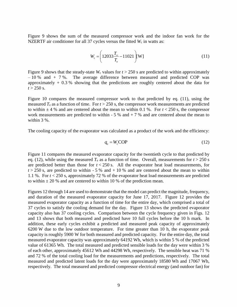
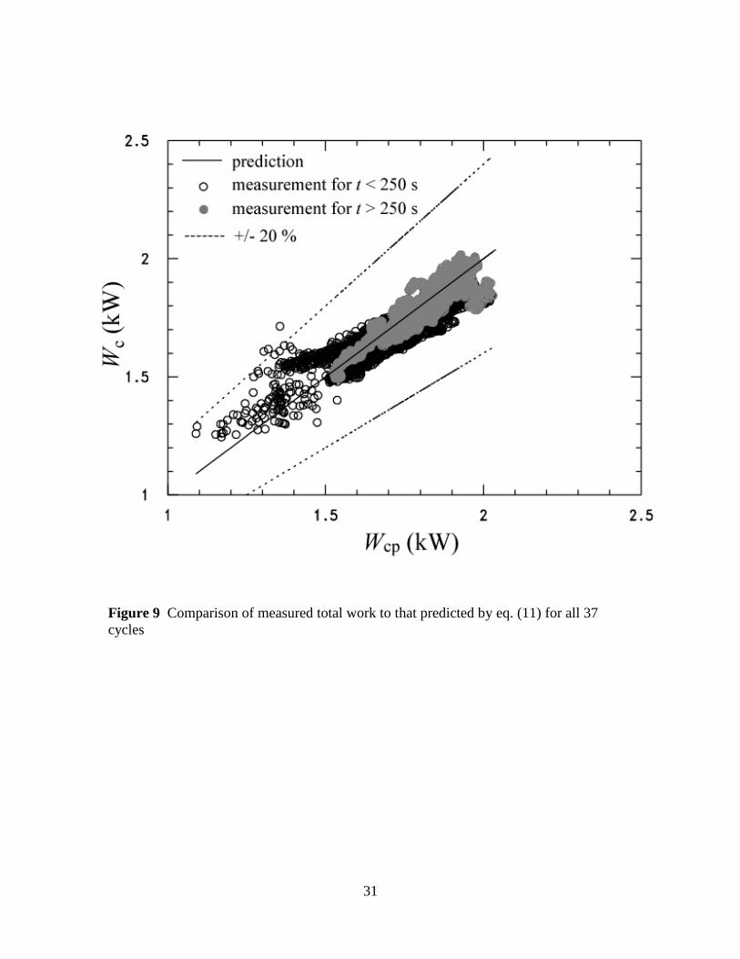
Figure 9 shows the sum of the measured compressor work and the indoor fan work for the

NZERTF air conditioner for all 37 cycles versus the fitted Wc in watts as:

c

e

12033 11021 [W]T

WT

(11)

Figure 9 shows that the steady-state Wc values for t > 250 s are predicted to within approximately

– 10 % and + 7 %. The average difference between measured and predicted COP was

approximately + 0.3 % showing that the predictions are roughly centered about the data for

t > 250 s.

Figure 10 compares the measured compressor work to that predicted by eq. (11), using the

measured Te as a function of time. For t > 250 s, the compressor work measurements are predicted

to within ± 4 % and are centered about the mean to within 0.1 %. For t < 250 s, the compressor

work measurements are predicted to within - 5 % and + 7 % and are centered about the mean to

within 3 %.

The cooling capacity of the evaporator was calculated as a product of the work and the efficiency:

e cCOPq W (12)

Figure 11 compares the measured evaporator capacity for the twentieth cycle to that predicted by

eq. (12), while using the measured Te as a function of time. Overall, measurements for t > 250 s

are predicted better than those for t < 250 s. All the evaporator heat load measurements, for

t > 250 s, are predicted to within - 5 % and + 10 % and are centered about the mean to within

1.1 %. For t < 250 s, approximately 72 % of the evaporator heat load measurements are predicted

to within ± 20 % and are centered to within 10 % of the prediction mean.

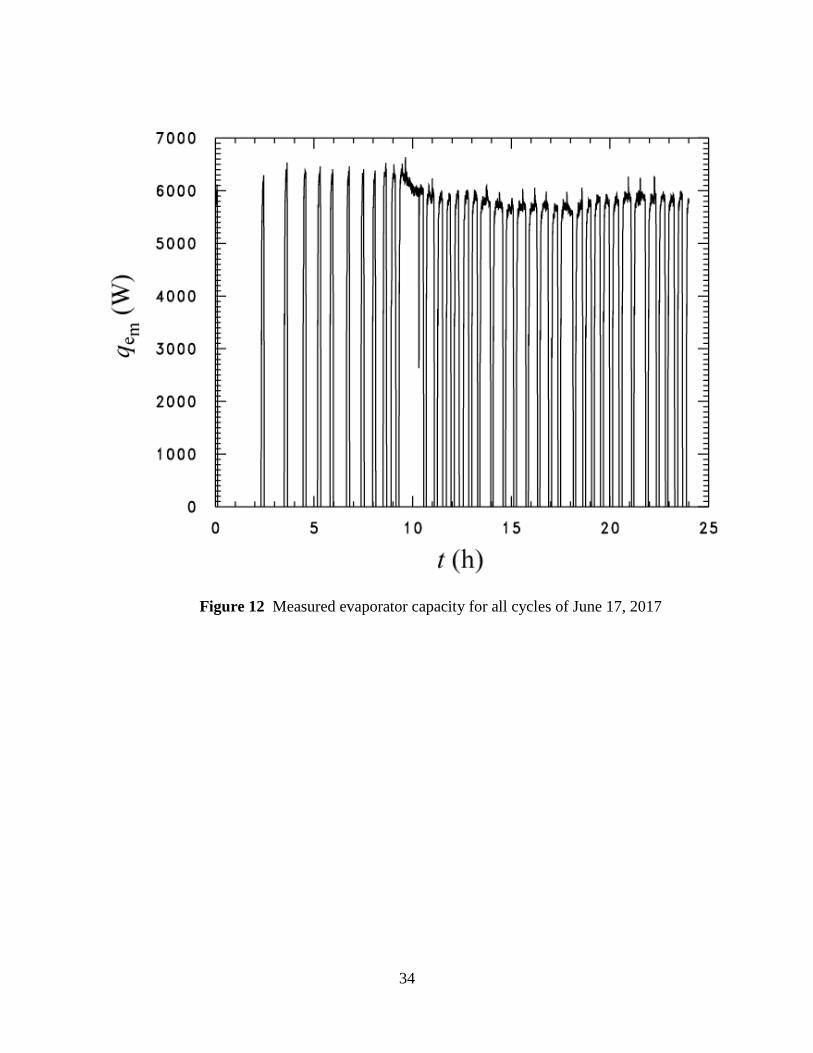
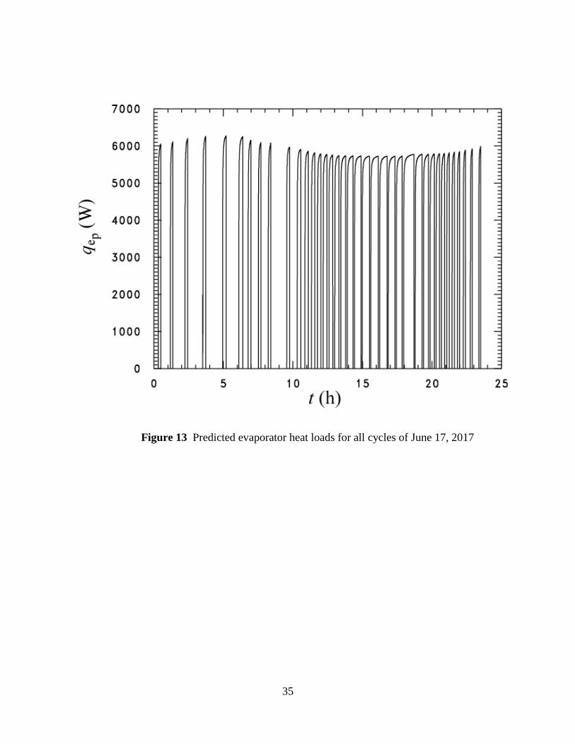
Figures 12 through 14 are used to demonstrate that the model can predict the magnitude, frequency,

and duration of the measured evaporator capacity for June 17, 2017. Figure 12 provides the

measured evaporator capacity as a function of time for the entire day, which comprised a total of

37 cycles to satisfy the cooling demand for the day. Figure 13 shows the predicted evaporator

capacity also has 37 cooling cycles. Comparison between the cycle frequency given in Figs. 12

and 13 shows that both measured and predicted have 10 full cycles before the 10 h mark. In

addition, these early cycles exhibit a predicted and measured peak capacity of approximately

6200 W due to the low outdoor temperature. For time greater than 10 h, the evaporator peak

capacity is roughly 5900 W for both measured and predicted capacity. For the entire day, the total

measured evaporator capacity was approximately 64192 Wh, which is within 5 % of the predicted

value of 61365 Wh. The total measured and predicted sensible loads for the day were within 3 %

of each other, approximately 45612 Wh and 44298 Wh, respectively. The sensible heat was 71 %

and 72 % of the total cooling load for the measurements and predictions, respectively. The total

measured and predicted latent loads for the day were approximately 18580 Wh and 17067 Wh,

respectively. The total measured and predicted compressor electrical energy (and outdoor fan) for

10

the day were within 1.5 % of each other being approximately 19378 Wh and 19632 Wh,

respectively.

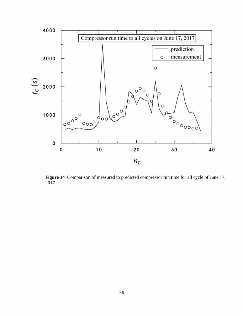
Figure 14 compares the measured to the predicted compressor run time (tc) for each numbered

cycle (nc). The figure shows that 20 out of the 37 cycle run times are predicted to within 200 s.

Nearly half of the remaining run times are predicted to within 400 s.

MODELING WITH PCM ENERGY STORAGE

The previous section presented and validated the model for predicting the transient cooling

performance of the NZERTF for June 17, 2017. This section discusses how that model was

modified in order to predict how PCM energy storage would affect the cooling performance of the

NZERTF. This section examines three different PCM energy storage concepts: integrated PCM,

remote PCM, and remote PCM with PCM liquid-line subcooling.

Integrated PCM

Figure 15 shows the proposed integrated PCM evaporator that was analyzed. The PCM evaporator

resembles a conventional residential evaporator in that it is a tube-and-plate-fin geometry with air

flowing between the aluminum plate fins and evaporating refrigerant flowing inside nominally

9 mm OD copper tubes. The refrigerant tubes are inside larger copper tubes thus forming annuli

that are filled with PCM (integrated PCM). The total tubing length was set to double (140.8 m)

that of the existing evaporator to provide for a larger mass of PCM while keeping the size of the

evaporator small enough to realistically fit within typical residential indoor air-handlers. For the

same reason, the outer diameter of the evaporator tube that contained the PCM was chosen to be

0.0254 m. This configuration gives a total mass of PCM of approximately 53.65 kg. The melting

temperature of the PCM was chosen to be at the average evaporator temperature of the base case

evaporator. Consequently, the average refrigerant temperature of the evaporator, while it is

freezing the PCM, was chosen to be 5 K less than the PCM phase-change temperature (Tpe = 282

K). The PCM does not flow in the annulus, rather, each tube is closed on both ends. The specific

heat of the solid PCM and the thermal conductivity of the solid PCM at the freezing temperature

were 1380 J·kg-1K-1, and 1.09 W·m-1K-1, respectively.

The main limiting factor for the integral PCM design is the thickness of the annulus. The annulus

thickness controls? the resistance to heat transfer for freezing the PCM and also the heat transfer

resistance for melting the PCM to achieve cooling. Consequently, the smaller the annulus space

is, the smaller the heat transfer resistance of the PCM. However, the capacity for energy storage

is reduced as the annulus space is reduced. The rest time between cycles dictates the annulus space

because freezing the PCM is a transient process. Shamsundar and Sparrow (1974) developed an

analytical solution for this transient heat transfer problem. Equation (13) shows their solution for

the time (t) to freeze based on a dimensionless radius, = r/ro:

2 2

"

o p p o

1 1 1 1 11 1 1 4Ste ln 2Ste exp erf 2 ln erf

2 2 4 2Ste 2Ste 2Ste

2 /t

q r

(13)

11

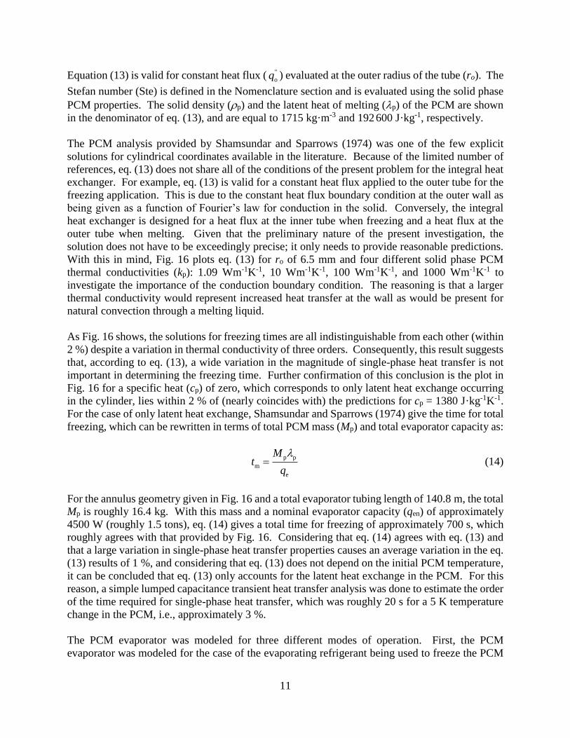
Equation (13) is valid for constant heat flux ( "

oq ) evaluated at the outer radius of the tube (ro). The

Stefan number (Ste) is defined in the Nomenclature section and is evaluated using the solid phase

PCM properties. The solid density (p) and the latent heat of melting (p) of the PCM are shown

in the denominator of eq. (13), and are equal to 1715 kg·m-3 and 192 600 J·kg-1, respectively.

The PCM analysis provided by Shamsundar and Sparrows (1974) was one of the few explicit

solutions for cylindrical coordinates available in the literature. Because of the limited number of

references, eq. (13) does not share all of the conditions of the present problem for the integral heat

exchanger. For example, eq. (13) is valid for a constant heat flux applied to the outer tube for the

freezing application. This is due to the constant heat flux boundary condition at the outer wall as

being given as a function of Fourier’s law for conduction in the solid. Conversely, the integral

heat exchanger is designed for a heat flux at the inner tube when freezing and a heat flux at the

outer tube when melting. Given that the preliminary nature of the present investigation, the

solution does not have to be exceedingly precise; it only needs to provide reasonable predictions.

With this in mind, Fig. 16 plots eq. (13) for ro of 6.5 mm and four different solid phase PCM

thermal conductivities (kp): 1.09 Wm-1K-1, 10 Wm-1K-1, 100 Wm-1K-1, and 1000 Wm-1K-1 to

investigate the importance of the conduction boundary condition. The reasoning is that a larger

thermal conductivity would represent increased heat transfer at the wall as would be present for

natural convection through a melting liquid.

As Fig. 16 shows, the solutions for freezing times are all indistinguishable from each other (within

2 %) despite a variation in thermal conductivity of three orders. Consequently, this result suggests

that, according to eq. (13), a wide variation in the magnitude of single-phase heat transfer is not

important in determining the freezing time. Further confirmation of this conclusion is the plot in

Fig. 16 for a specific heat (cp) of zero, which corresponds to only latent heat exchange occurring

in the cylinder, lies within 2 % of (nearly coincides with) the predictions for cp = 1380 J·kg-1K-1.

For the case of only latent heat exchange, Shamsundar and Sparrows (1974) give the time for total

freezing, which can be rewritten in terms of total PCM mass (Mp) and total evaporator capacity as:

p p

m

e

Mt

q

(14)

For the annulus geometry given in Fig. 16 and a total evaporator tubing length of 140.8 m, the total

Mp is roughly 16.4 kg. With this mass and a nominal evaporator capacity (qen) of approximately

4500 W (roughly 1.5 tons), eq. (14) gives a total time for freezing of approximately 700 s, which

roughly agrees with that provided by Fig. 16. Considering that eq. (14) agrees with eq. (13) and

that a large variation in single-phase heat transfer properties causes an average variation in the eq.

(13) results of 1 %, and considering that eq. (13) does not depend on the initial PCM temperature,

it can be concluded that eq. (13) only accounts for the latent heat exchange in the PCM. For this

reason, a simple lumped capacitance transient heat transfer analysis was done to estimate the order

of the time required for single-phase heat transfer, which was roughly 20 s for a 5 K temperature

change in the PCM, i.e., approximately 3 %.

The PCM evaporator was modeled for three different modes of operation. First, the PCM

evaporator was modeled for the case of the evaporating refrigerant being used to freeze the PCM

12

during times that cooling was not called for by the thermostat. The second case was when the

frozen PCM was used for cooling while the compressor was off. For this case, the PCM was

assigned a nominal heat duty of qen. The third case that was modeled was when the evaporating

refrigerant cooled the air while the PCM was liquid. Predictions were made for both the heat duty

and the mass of frozen PCM.

For the first and second PCM modes, because the annulus had a fixed mass of PCM, the mass of

frozen PCM was modeled by modeling the time remaining for the PCM to completely thaw (tt):

et c 1

en

1q

t t fq

(15)

If the PCM were frozen at the same rate as it was used to cool, and if none of the qe were required

for single phase heat transfer to the PCM (all cooling capacity went to freezing the PCM), then the

time to thaw would be equal to the total compressor run time: tt = tc. This not being the case, eq.

(15) required two correction factors to account for these effects. The fraction of total heat transfer

that goes to single phase heat transfer was accounted for with f1. For the annulus shown in Fig.16,

f1 was set to 0.04, which came from the sum of the 1 % difference exhibited between the zero and

the non-zero heat capacity eq. (13) solution and the 3 % difference between the eq. (13) solution

and the single-phase-heat-transfer-lumped-capacitance approximation. The ratio qe /qen was used

to account for the PCM freezing occurring at qe rather than the nominal heat flux (qen). Equation

(12) was used to calculate the qe based on the outdoor temperature and a 5 K lower evaporator

temperature that was required to freeze the PCM.

The total PCM cooling duty (qp) was the sum of the sensible cooling (qps) and the latent cooling

(qpl). The (qp) was the sum of the sensible cooling (qps) when the evaporator temperature was less

than the air temperature (Ta) and the dew-point temperature (Td), respectively. The sensible

cooling load was calculated for tt > 0 (when frozen PCM is available) from:

-1

ps a w d

1506 W K

2q T T T

(16)

The leading constant shown in eq (16) was obtained from the sensible heat transfer hA of the base

case. This was done to ensure the same sensible heat transfer characteristics as the base case,

which is equivalent to adjusting the airflow rate until the same sensible behavior is achieved. The

sensitivity of the leading constant was analyzed by increasing it in steps of roughly 500 WK-1 up

to 4500 WK-1, which did not change the total heat load for the day by more than 1 %.

The latent cooling load was calculated for tt > 0 from eq. (4) as:

-1

pl d e1592.42 W K 5935.73[W]q T T (17)

where the wall temperature of the evaporator (Te) was derived from a simple cylindrical conduction

model as:

13

ps e p -1

d

p

o

ee p

p

o

0.61592.42 W K 5935.73[W]

ln

0.61592.42

ln

T L kT

r

rT

L k

r

r

(18)

Equation (18) considers the temperature drop that occurs from the phase-change interface radius

(rp) to the outer radius (ro) of the PCM. Equation (18) is a conservative estimate because the

subcooling of the PCM is neglected, whereas, the frozen PCM is assumed to be at the melting

temperature (Tps).

The air-side latent cooling load (ql) while the compressor was running with no PCM cooling load

was calculated for tt < 0 from an energy balance as:

2 2

p i o i o1

l d ps p

i o

ln 1 / /

1592.42 W K 5935.73 Wln /

f r r r r

q T T Tr r

(17)

fp is the fraction of the total PCM mass that is frozen in annulus. Equation (17) accounts for the

additional resistance to heat transfer due to the presence of the PCM in the annulus.

While the PCM was used to cool, the system work was set equal to the indoor fan work of 125 W

because during this time the compressor was off.

For the third mode of heat exchange with the PCM evaporator, the cooling duty (qec) was reduced

due to the heat transfer resistance through the liquid PCM within the annulus as:

st e

ec e

st e p

T Tq q

T T T

(18)

where Tst was the setpoint temperature of the thermostat. The value of qe was calculated from eq.

(12). The temperature drop across the PCM annulus (Tp) was calculated with a steady-state

conduction model. The average temperature of the evaporator at the outer refrigerant tube wall

(Te) was set to the average measured value of 282.2 K. The average evaporator temperature for

this case was increased only if the system was unable to satisfy the setpoint temperature.

14

The latent cooling heat duty with the evaporating refrigerant when the PCM was liquid was

reduced for the case of the evaporator having PCM within the annulus due to the higher surface

temperature, which was larger by Tp:

1

d e p2 1592.42 W K 5935.73 Wq T T T (19)

For fixed evaporator surface area, Park et al. (2001) have shown that the efficiency of a residential

AC increases approximately linearly as the compressor frequency () is reduced from 90 Hz to 30

Hz. For example, the efficiency was shown to increase by approximately 36 % when the

compressor frequency was reduced from 60 Hz to 30 Hz. The improved system performance

(COPI) associated with an effectively smaller nominal compressor tonnage, which was obtained

from the Park et al. (2001) measurements, were fitted to the baseline COP and their respective

frequencies as:

IICOP COP 1 K K

(20)

where the constant K is equal to 0.722 and 1.696 for base compressor frequencies () of 60 Hz

and 90 Hz, respectively. To reproduce the Park et al. (2001) data, the base COP for eq. (20) is

approximately 3.6 and 2.3 for a of 60 Hz and 90 Hz, respectively.

If the purpose of eq. (20) was merely to reproduce the Park et al. (2001) measurements, then COPI

would have simply been a linear function of I, with the baseline COP and being omitted from

the fit. Using ratios of the system performances and ratios of the frequencies in eq. (20), allowed

the frequency ratio to be replaced by the nominal tonnage ratio of the compressors, i.e., I/ =

NI/N. In this way, the efficiency of the NZERTF could be adjusted to account for reduced

compressor tonnage without being bound to the absolute value of the Park et al. (2001) system

performance. In addition, the form of eq. (20) allows the comparison of two different performance

enhancements by comparing the results for two different values of K. The smaller value of K

approximates the improvement in the system performance by reducing only the compressor size

while fixing the size of the evaporator. The larger value of K approximates the improvement in

system performance for simultaneous reduction of the compressor size and doubling of the

evaporator surface area.4 This is the case for the integrated PCM where in addition to operating at

a lower compressor tonnage, the PCM evaporator has double the heat transfer surface area of that

of the base case. Corresponding to the larger K, both effects act to improve the efficiency as

compared to the base case.

The base case system efficiency (COP) that was used in eq. (20) was taken from eq. (8). The

system performance of the PCM system was calculated from eq. (20) by using the appropriate

nominal compressor tonnage ratio. The PCM system used a two-speed compressor to take

advantage of the larger system efficiencies at lower outdoor temperatures. During non-peak times,

a 50 % larger compressor tonnage was used when the system was used to freeze the PCM.

4 The latent load is calculated based on the average surface temperature of the evaporator.

15

Figure 17 shows the house air temperature as a function of time of day while using the PCM

evaporator described above and a 1 ton, two-speed compressor for two different values of K. The

solid line and the dashed line represent K values of 1.696 and 0.722, respectively. The choice of

the 1 ton compressor was a compromise between meeting the peak load of the day and increasing

the efficiency as a consequence of longer run times. For K = 1.696, the figure shows that the

compressor experienced 29 run cycles, which is approximately a 22 % reduction as compared to

the base case (37 cycles), and that the integrated PCM evaporator system satisfied the setpoint

temperature throughout the day. Conversely, for K = 0.722, the integrated PCM evaporator system

was unable to meet the setpoint temperature between 13.9 h and 22.2 h where the setpoint was

exceeded by approximately 3 K, and during a peak of 300.5 K near 19 h. For the entire day, the

total measured evaporator capacity was approximately 60913 Wh (K = 1.696) and 57883 Wh (K

= 0.722), which was approximately 1 % and 6 % less, respectively, than the base case with the

2 ton compressor and no PCM. The total sensible load for the day was within 1 % and 6 % of the

base case being approximately 44204 Wh (K = 1.696) and 41479 Wh (K = 0.722), respectively.

The total latent loads for the integrated evaporator was within 3 % and 4 % of the base case being

approximately 16544 Wh (K = 1.696) and 16437 Wh (K = 0.722), respectively. The integrated

PCM evaporator roughly offered a 37 % (K = 1.696) and a 26 % (K = 0.722) energy savings over

the base case. The total system energy values for the day with the integrated PCM evaporator with

K = 1.696 and K = 0.722 were approximately 12320 Wh and 14515 Wh, respectively.

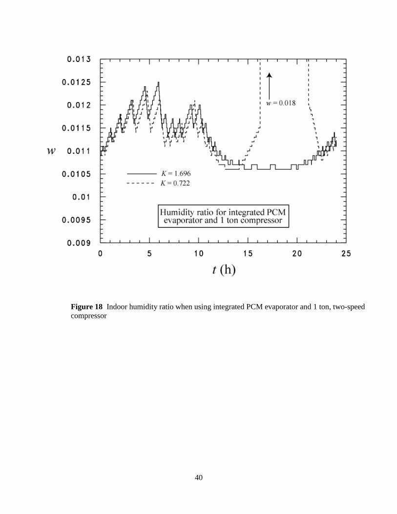
Figure 18 shows that the indoor humidity ratio (a partial indicator of thermal comfort) produced

by the integrated PCM system, while assuming a K = 1.696, was acceptable because the humidity

ratio was less than 0.012 and the temperature was within the setpoint for most of the day. As

compared to humidity ratio for the base case shown in Fig. 2, the humidity ratio produced by the

integrated PCM evaporator with K = 1.696 is roughly 6 % larger. The larger humidity ratio is due

to the higher evaporator surface temperatures caused by the thermal resistance of the PCM. This

effect could be reduced by designing a system that operated at a lower phase-change temperture;

however, the lower PCM temperature would necessitate greater system energy input. For the

lower system efficiency (K = 0.722), Fig. 18 shows that the humidity ratio is approximately the

same as that of the higher efficiency system (K = 1.696) except during peak hours where the PCM

has been spent and the compressor is not large enough to meet the load.

Table 1 Effect of PCM mass on system performance

ro (mm) K Mp (kg) tm (s) Sensible

(Wh)

Latent

(Wh)

Total

work

(Wh)

Peak Ta

(K)

4.45 0.722 0 0 42162 17394 13030 299.6

4.45 1.696 0 0 44259 17170 10528 297.5

5.00 1.696 3.6 231 44290 16905 10862 297.5

6.47 0.722 16.4 1052 41479 16436 14515 300.5

6.47 1.696 16.4 1052 44204 16543 12320 297.5

8.00 1.696 33.2 2131 44214 16522 13263 297.5

9.00 1.696 46.0 2959 44039 16099 13569 297.5

10.00 1.696 60.5 3884 44061 16253 13656 297.5

12.7 1.696 107.0 6869 43722 15539 13851 298.0

16

Table 1 illustrates the effect of PCM mass (Mp) within the evaporator by varying the outer radius

(ro) of the evaporator tube. For the same K, each simulation shown in Table 1 exhibited similar

latent and sensible heat transfer characteristics. The last column shows the maximum indoor air

temperature experienced during peak cooling times, where a value of 297.5 indicates that the

systems satisfied the indoor air temperature setpoint throughout the day. In general, the analysis

shows that because of the heat transfer resistance through the PCM, adding more PCM in order to

achieve increased energy storage results in increased work input and therefore reduced energy

efficiency. In fact, the K = 1.696 systems with the best performances are the two with the smallest

PCM masses: 3.6 kg and 0 kg. These systems have 44 % and 46 % less energy input requirements

than the base 2 ton system. The humidity ratios for both the 3.6 kg and the 0 kg PCM system

remain mainly below 0.012 during the peak hours while maintaining the indoor air temperature

within the setpoint limits. Consequently, for the current integrated PCM evaporator system design,

there is no advantage over a high-efficiency system without a PCM that achieves the high

efficiency by means of a 1 ton compressor and a doubling of the evaporator heat transfer surface

area. There are two reasons for this result. First, the system without PCM requires approximately

3 % system work to meet the same heat transfer loads, indoor air temperatures, and humidity ratios.

Second, because the integrated PCM evaporator has no frozen PCM during the peak load hours

due to insufficient PCM mass in the annulus, there is minumal peak load shifting. As Table 1

shows, increasing ro and the PCM mass acts to increase the system power requirements with an

insufficient increase in the time of frozen PCM use (tm) during the peak hours. In addition, without

the added effect of increased system effciency due to the larger evaporators (systems with

K = 0.722), the indoor air temperature does not remain within the bounds of the setpoint. From

the above analysis, the present integrated PCM evaporator design is not a viable candidate for

residential energy storage due to the significant temperature gradients across the PCM in the

annulus and the lack of sufficient PCM mass to accomplish meaningful load shifting during peak

hours. To further emphasise that the integrated PCM evaporator as modelled provides no benefit,

Table 1 shows that more energy savings can be obtained by increasing the size of the evaporator

without the use of PCM while simultaneously reducing the size of the compressor.

Discrete PCM

To mitigate the effect of insufficient PCM mass, a second concept for the PCM evaporator locates

the PCM external to the air handler within its own heat exchanger (discrete PCM) as shown in

Fig. 19. Storing the PCM external to the evaporator eliminates the concern of having sufficient

PCM mass within a limited evaporator volume and footprint, but adds complexity as additional

valves are needed for control. Clarksean (2006) built and tested a mockup/benchtop apparatus to

test the concept of a PCM slurry to reduce residential air-conditioning peak loads. Clarksean

(2006) demonstrated that a PCM could be either cooled or heated and then pumped to a heat

exchanger to cool or heat air in a residential-like duct. Consequently, remote PCM air conditioning

could be achieved by pumping a PCM slurry. The advantage of such a configuration is that it

avoids the resistive heat transfer irreversibilities associated with using a secondary fluid. Further

efficiency losses could be avoided by using an immiscible, low vapor-pressure PCM in

conjunction with direct contact heat exchange between the refrigerant and the PCM.

In order to meet the NZERTF peak load cooling demand with only the PCM heat exchanger, it

was necessary to use approximately 935 kg of PCM storage. This value was obtained iteratively

17

with the discrete PCM analysis by observing the mass of PCM that was required to meet the entire

peak load. Using only the PCM to cool during peak hours, with the compressor turned off,

provides two key advantages over a conventional air-conditioning system. First, the system

efficiency is improved as compared to the base case because of the increase in the evaporator size

and because the PCM is frozen during off peak hours when the outdoor temperature is at its lowest

of the day. Second, only the blower power is used during peak hours, so that the electric utility

receives the benefit of load shedding. A two-speed system allows the compressor to be operated

at high speed while the PCM is being frozen and low speed while the indoor air is being cooled

during off-peak hours. The higher speed is used because not enough PCM could be frozen to meet

the peak load cooling with a single-speed, one-ton compressor.

The choice of the PCM system design determines the magnitude of the heat transfer

irreversibilities associated with charging (freezing) the PCM, and it determines the heat transfer

irreversibilities associated with transferring the cooling from the PCM to the air. Rather than

choosing a specific remote PCM system to model, the heat transfer resistance was varied to

simulate different remote PCM systems having different heat transfer resistances. With this in

mind, the same model that was used for the integrated PCM evaporator system was used with the

exception that the mass of PCM was not limited by eq. (14). The mass of the PCM for the remote

system was chosen such that there was sufficient PCM mass to meet the entire peak cooling load.

The fraction of total heat transfer that goes to single phase heat transfer (f1) and the ro were used

to account for the difference between a system that used a slurry PCM with direct contact heat

exchange (f1= 0.01 and ro = 6.47 mm) and one that used additional heat exchangers with an

additional heat transfer fluid (f1= 0.08 or larger and ro = 10.0 mm or larger). The ro was used to

set the distance between the PCM phase boundary and the heat transfer surface. For example, a

remote storage with a larger heat transfer surface area, would have a smaller effective ro, for a

fixed PCM mass, than one with less heat transfer surface area. In this way, the system with the

least heat transfer resistance (direct contact heat exchange between the refrigerant and PCM with

a PCM slurry being pumped through the air-heat exchanger) was effectively compared to systems

with larger heat transfer resistances that use secondary fluids and heat exchangers between the

PCM and the air and the PCM and the refrigerant.

Figure 20 shows the system work for the remote PCM for various heat transfer resistances as

represented by f1and ro for two values of K where a linear fit of the predictions is shown as a solid

line. The required system work for the 1 ton system with remote PCM is between roughly 13200

Wh and 18550 Wh, which is roughly a 33 % and a 6 % reduction, respectively, in the required

system energy of the 2 ton base case. Figure 20 shows that the required system work increases

linearly as the fraction of the total heat transfer that goes to single phase heat transfer increases.

For example, increasing f1 from 1 % to 25 % causes a corresponding 24 % and 27 % increase in

the required work for K = 0.722 and K = 1.696, respectively. Consequently, designing a system

so that most of the energy is stored as phase-change energy with little subcooling of the PCM is

crucial for an efficient energy storage design. For f1 = 1 %, the remote PCM system required

approximately 24 % and 33 % less system energy than that required for the 2 ton compressor base

case (19632 Wh), for K = 0.722 and K = 1.696, respectively. For f1 = 25 %, the remote PCM

system required approximately 6 % (K = 0.722) and 14 % (K = 1.696) less system energy than that

required for the base case. As Fig. 20 shows, the average reduction for the K = 0.722 and the

K = 1.696 systems was 15 % and 24 %, respectively.

18

Figure 20 shows that the variation in the value of ro causes a 5 % or less variation in the required

system work. For the remote storage analysis, the ro does not represent a physical diameter. Rather

ro approximates a region of influence for the PCM heat flux, which works to increase the surface

temperature of the air-heat exchanger (Fig. 19) during cooling and to reduce the total cooling

capacity. Figure 21 shows that less moisture removal occurs for the largest ro and the largest f1

as a result of the higher evaporator surface temperatures. However, Fig. 21 shows that the

humidity ratio mainly remains within the acceptable thermal comfort region of less than 0.012 for

the peak load hours. Consequently, care should be taken to ensure efficient heat exchange between

the air and the PCM so that adequate de-humidification is attained.

CONCLUSIONS

The successful marriage of a PCM with a vapor compression cycle has the potential to significantly

increase the efficiency of air-source vapor compression systems used for space conditioning,

which relies on a favorable system design. To investigate the efficacy of certain residential energy

storage designs, the air-conditioning performance, and the associated external and internal heat

loads to NIST’s Net-Zero Energy Residential Test Facility, were modelled for a single day near

the summer. Two types of residential air-conditioning systems were examined to determine the

energy savings and the peak load shifting that could be obtained by using PCM. The first type of

system limited the mass of the PCM to minimize the required changes to a conventional cooling

system. The main component of the first type of cooling system was the integrated PCM

evaporator where a limited amount of PCM was placed directly integral to the tube of the

evaporator within an annulus. The system with the integral PCM evaporator showed no potential

advantage over a conventional system without PCM but with a larger evaporator and a smaller

compressor. The system with the integral PCM evaporator failed to deliver energy savings and

peak load shifting due to insufficient PCM and heat transfer resistance through the PCM held

within the annulus. In contrast, the second type of residential cooling system, which used remotely

stored PCM, exhibited significant energy savings while shifting the entire peak load to PCM heat

exchanger with minimal electricity use during the peak load hours. In addition, the remote PCM

system achieved between a 6 % and a 33 % reduction in the required energy for the entire cooling

day, while maintaining acceptable indoor humidity ratios. The performance was best when the

heat transfer resistance was minimized with direct contact heat exchange between the PCM and

the evaporating refrigerant.

ACKNOWLEDGEMENTS

This work was funded by NIST. Thanks go to Dr. Riccardo Brignoli of the University of Padova

and to Brian Dougherty and Piotr Domanski of NIST for their constructive criticism of the draft

manuscript.

19

NOMENCLATURE

English symbols

A heat transfer surface area (m-2)

Bn fitting constants; n = 0 or 1 (-)

cpa specific heat of moist air inside house (kJ·kg-1·K-1)

EST energy stored in the air (W)

f1 fraction of total load that is single-phase heat transfer (-)

fp fraction of total PCM mass that is frozen in annulus (-)

h heat transfer coefficient (W·m-2·K-1) hA heat conductance (W·K-1)

ifg latent heat of vaporization of water (kJ·kg-1)

Is solar irradiance (W·m-2)

kp thermal conductivity of PCM (W·m-1·K-1)

K system efficiency constant in eq. (20) (-)

Le total length of heat exchanger tubing (m)

M mass (kg)

Ma total mass of dry air inside house (kg)

nc number of cycles

N nominal number of compressor tons (-)

P pressure (Pa)

r radial coordinate for tube with center origin (m)

ri inner tube annulus radius (m)

ro outer tube radius (m)

t time (s)

tc compressor run time (s)

tt PCM time to total thaw (s)

T temperature (K)

Ta air temperature (K)

Tpe PCM phase-change temperature (K)

Tst setpoint temperature of the thermostat (K)

T outdoor temperature (K)

qe evaporator heat duty (W)

qec evaporator heat duty reduced by PCM resistance (W)

qg plug load for the house (W)

ql evaporator air-side latent load (W)

qp total PCM evaporator duty (W)

qpl PCM evaporator latent duty (W)

qps PCM evaporator sensible duty (W)

qs heat transfer from sun to house (W)

qUA heat transfer through walls driven by T - Tai (W) "

oq heat flux to outer tube (W·m-2)

Ste Stefan number,

"

p o oc q r

k(-)

UA overall conductance of house exterior thermal envelope, walls, roof and windows (W·K-1)

w humidity ratio (kg water vapor/kg dry air)

W electrical work (W)

20

Greek symbols

P pressure drop (kPa)

Tp temperature drop across the PCM annulus ()

p latent heat of melting (J·kg-1)

dimensionless radius; = r/ro (-)

p PCM solid density (kg·m-3)

time constant (s-1)

indoor relative humidity (-)

frequency (s-1)

Subscripts

1 sensible load

2 latent load

c outdoor unit and indoor fan, cycle

d dew point

e evaporator

f fan

i indoor

I improved

m measured, maximum

n nominal

o outdoor, at outer tube wall

p predicted

PC phase change

r house roof

s solar

w house wall

WN house window

Abbreviations

AC Air Conditioning

ASHP air-source heat pump

COP Coefficient of Performance

HRV Heating Recovery Ventilator

NIST National Institute of Standards and Technology (in U.S. Dept. of Commerce)

NZERTF Net-Zero Energy Residential Test Facility at NIST

OD Outer Diameter

PC Phase Change

PCM Phase-change Material

PV Photovoltaic

SHGC Solar Heat Gain Coefficient

TES Thermal Energy Storage

U.S. United States

21

REFERENCES

ASHRAE. 2017. ANSI/ASHRAE Standard 55-2017, Thermal Environmental Conditions for

Human Occupancy.

ASHRAE. 2015. 2015 ASHRAE Handbook -HVAC Systems and Equipment, Chapter 51,

Atlanta, GA, p. 51-1.

Baxter, V.D., and Moyers, J.C. 1985. Field-measured cycling, frosting, and defrosting losses for

a high-efficiency air-source heat pump. ASHRAE Trans. Vol. 91:2B. 537-554.

Davis, M. W., Healy, W.M., Boyd, Ng., L, W. V., Payne, W.V. Skye, H., L., and Ullah, T.

2014. Monitoring Techniques for the Net-Zero Energy Residential Test Facility, NIST Technical

Note 1854. U.S. Department of Commerce, Washington, D.C.,

http://dx.doi.org/10.6028/NIST.TN.1854

Incropera, F. P., and DeWitt, D. P. 2002. Fundamentals of Heat and Mass Transfer, 5th ed., John

Wiley & Sons, New York.

Clarksean, R. 2006. A phase change material slurry system to decrease peak air-conditioning

loads, California Energy Commission, publication CEC-500-2006-026.

Kedzierski, M. A., Payne, W. V., and Skye, H. M. 2014. Potential Research Areas in Residential

Energy Storage for NIST’s Engineering Laboratory, NIST Technical Note 1844, U.S.

Department of Commerce, Washington, D.C.

Kumano, H., Asaoka, T., and Sawada, S. 2014. Effect of Initial Aqueous Solution Concentration

and Heating Conditions on Heat Transfer Characteristics of Ice Slurry, Int. J. Refrigeration, Vol.

41, pp. 72-81.

Lstiburek, J. W. 2010. The Perfect Wall, buildingscience.com, BSC: BSI-001,

http://www.buildingscience.com/index_html.

Lo´pez-Navarro, A., Biosca-Taronger, J., Torregrosa-Jaime, B., Martı´nez-Galva´, I.,Corbera´ J.

M., Esteban-Matı´ J.C., and Paya´, J. 2013. Experimental Investigation of the Temperatures and

Performance of a Commercial Ice-Storage Tank, Int. J. Refrigeration, Vol. 36, pp. 1313-1318.

Omar, F. 2017. Private communications. National Institute of Standards and Technology.

Gaithersburg, MD.

Omar, F., Bushby, S. T., and Williams, R. D. 2017. A self-learning algorithm for estimating solar

heat gain and temperature changes in a single-family residence. Energy and Buildings. 150, 100–

110. http://dx.doi.org/10.1016/j.enbuild.2017.06.001

Park. Y. C., Kim, Y. C., and Min, M. 2001. Performance analysis on a multi-type inverter air

conditioner, Energy Conversion and Management, 42, 1607-1621.

http://dx.doi.org/10.1016/j.enbuild.2017.06.001

22

Pettit, B., Gates, C. Fanney, A. H., and Healy, W. M. 2015. Design Challenges of the NIST Net

Zero Energy Residential Test Facility. NIST Technical Note 1847, U.S. Department of

Commerce, Washington, D.C. https://dx.doi.org/10.6028/NIST.TN.1847

Shamsundar, N., and Sparrow, E. M. 1974. Storage of Thermal Energy by Solid-Liquid Phase

Change-Temperature Drop and Heat Flux, ASME J. Heat Transfer, 96(4):541-544.

doi:10.1115/1.3450242.

23

Figure 1 Outdoor temperature for June 17, 2017

Figure 2 Energy balance for NZERTFFigure 1 Outdoor

temperature for June 17, 2017

Figure 2 Energy balance for NZERTF

Figure 3 Humidity ratio for the NZERTF on June 17,

2017Figure 2 Energy balance for NZERTFFigure 1 Outdoor


Figure 2 Energy balance for NZERTFFigure 1 Outdoor


24

Figure 2 Energy balance for NZERTF


2017Figure 2 Energy balance for NZERTF


2017

Figure 4 Plug loads for NZERTF on June 17,

2017Figure 3 Humidity ratio for the NZERTF on June

17, 2017Figure 2 Energy balance for NZERTF


2017Figure 2 Energy balance for NZERTF

25

Figure 3 Humidity ratio for the NZERTF on June 17, 2017

Figure 4 Plug loads for NZERTF on June 17, 2017Figure 3

Humidity ratio for the NZERTF on June 17, 2017

Figure 4 Plug loads for NZERTF on June 17, 2017

Figure 5 Solar heat gain for June 17, 2017Figure 4 Plug loads for

NZERTF on June 17, 2017Figure 3 Humidity ratio for the NZERTF

on June 17, 2017

Figure 4 Plug loads for NZERTF on June 17, 2017Figure 3

Humidity ratio for the NZERTF on June 17, 2017

26

.

Figure 4 Plug loads for NZERTF on June 17, 2017

Figure 5 Solar heat gain for June 17, 2017Figure 4

Plug loads for NZERTF on June 17, 2017

Figure 5 Solar heat gain for June 17, 2017

Figure 6 NZERTF air-source heat pump schematic

(Davis et al., 2014)Figure 5 Solar heat gain for June

17, 2017Figure 4 Plug loads for NZERTF on June 17,

2017

Figure 5 Solar heat gain for June 17, 2017Figure 4

Plug loads for NZERTF on June 17, 2017

27

Figure 5 Solar heat gain on June 17, 2017



17, 2017


(Davis et al., 2014)

Figure 7 COP for 20th cycle for June 17, 2017Figure 6

NZERTF air-source heat pump schematic (Davis et al.,

2014)Figure 5 Solar heat gain for June 17, 2017



17, 2017

28

Figure 6 NZERTF air-source heat pump schematic (Davis et al., 2014)

Figure 7 COP for 20th cycle for June 17, 2017Figure 6 NZERTF air-

source heat pump schematic (Davis et al., 2014)

Figure 7 COP for 20th cycle for June 17, 2017

Figure 8 Comparison of measured COP to eq. (3) for all 37 cyclesFigure

7 COP for 20th cycle for June 17, 2017Figure 6 NZERTF air-source heat

pump schematic (Davis et al., 2014)

Figure 7 COP for 20th cycle for June 17, 2017Figure 6 NZERTF air-

source heat pump schematic (Davis et al., 2014)

29

Figure 7 COP for 20th cycle on June 17, 2017

Figure 8 Comparison of measured COP to eq. (3) for all

37 cyclesFigure 7 COP for 20th cycle for June 17, 2017


37 cycles

Figure 9 Comparison of measured compressor work to

eq. (11) for all 37 cyclesFigure 8 Comparison of

measured COP to eq. (3) for all 37 cyclesFigure 7 COP

for 20th cycle for June 17, 2017


37 cyclesFigure 7 COP for 20th cycle for June 17, 2017

30

Figure 8 Comparison of measured COP to that predicted with eq. (3) for all 37 cycles

Figure 9 Comparison of measured compressor work to eq. (11) for all 37 cyclesFigure

8 Comparison of measured COP to eq. (3) for all 37 cycles

Figure 9 Comparison of measured compressor work to eq. (11) for all 37 cycles

Figure 10 Comparison of measured compressor work to eq. (11) for 20th cycle for June

17, 2017Figure 9 Comparison of measured compressor work to eq. (11) for all 37

cyclesFigure 8 Comparison of measured COP to eq. (3) for all 37 cycles

Figure 9 Comparison of measured compressor work to eq. (11) for all 37 cyclesFigure

8 Comparison of measured COP to eq. (3) for all 37 cycles

31

Figure 9 Comparison of measured total work to that predicted by eq. (11) for all 37

cycles

32

Figure 10 Comparison of measured compressor and fan work that predicted with eq. (11) for

20th cycle on June 17, 2017

Figure 12 Measured evaporator heat loads for all cycles of June 17, 2017Figure 11 Comparison

of measured evaporator heat load to eq. (12) for 20th cycle for June 17, 2017Figure 10

Comparison of measured compressor work to eq. (11) for 20th cycle for June 17, 2017

Figure 11 Comparison of measured evaporator heat load to eq. (12) for 20th cycle for June 17,

2017Figure 10 Comparison of measured compressor work to eq. (11) for 20th cycle for June 17,

2017

33

Figure 11 Comparison of measured evaporator capacity to that predicted with eq. (12) for

20th cycle on June 17, 2017

Figure 12 Measured evaporator heat loads for all cycles of June 17, 2017Figure 11

Comparison of measured evaporator heat load to eq. (12) for 20th cycle for June 17, 2017

Figure 12 Measured evaporator heat loads for all cycles of June 17, 2017

Figure 13 Predicted evaporator heat loads for all cycles of June 17, 2017Figure 12

Measured evaporator heat loads for all cycles of June 17, 2017Figure 11 Comparison of

measured evaporator heat load to eq. (12) for 20th cycle for June 17, 2017

Figure 12 Measured evaporator heat loads for all cycles of June 17, 2017Figure 11

Comparison of measured evaporator heat load to eq. (12) for 20th cycle for June 17, 2017

34

Figure 12 Measured evaporator capacity for all cycles of June 17, 2017


Measured evaporator heat loads for all cycles of June 17, 2017

Figure 13 Predicted evaporator heat loads for all cycles of June 17, 2017

Figure 14 Comparison of measured to predicted compressor run time for all cycle of June 17,

2017Figure 13 Predicted evaporator heat loads for all cycles of June 17, 2017Figure 12




35

Figure 13 Predicted evaporator heat loads for all cycles of June 17, 2017


2017Figure 13 Predicted evaporator heat loads for all cycles of June 17, 2017


2017

Figure 15 Proposed PCM evaporator for investigation (Kedzierski et al., 2014)Figure 14

Comparison of measured to predicted compressor run time for all cycle of June 17,




36


2017


Comparison of measured to predicted compressor run time for all cycle of June 17, 2017

Figure 15 Proposed PCM evaporator for investigation (Kedzierski et al., 2014)

Figure 16 Shamsundar and Sparrow (1974) model for freezing and melting time for

PCMFigure 15 Proposed PCM evaporator for investigation (Kedzierski et al., 2014)Figure

14 Comparison of measured to predicted compressor run time for all cycle of June 17, 2017


Comparison of measured to predicted compressor run time for all cycle of June 17, 2017

37

Figure 15 Proposed PCM evaporator for investigation (Kedzierski et al., 2014)


PCMFigure 15 Proposed PCM evaporator for investigation (Kedzierski et al., 2014)

Figure 16 Shamsundar and Sparrow (1974) model for freezing and melting time for PCM

Figure 17 Indoor air temperature when using integrated PCM evaporator and 1-ton two-

speed compressorFigure 16 Shamsundar and Sparrow (1974) model for freezing and melting

time for PCMFigure 15 Proposed PCM evaporator for investigation (Kedzierski et al., 2014)


PCMFigure 15 Proposed PCM evaporator for investigation (Kedzierski et al., 2014)

38


PCM

Figure 17 Indoor air temperature when using integrated PCM evaporator and 1-ton

two-speed compressorFigure 16 Shamsundar and Sparrow (1974) model for freezing

and melting time for PCM


two-speed compressor

Figure 18 Indoor humidity ratio when using integrated PCM evaporator and 1-ton,

two-speed compressorFigure 17 Indoor air temperature when using integrated PCM

evaporator and 1-ton two-speed compressorFigure 16 Shamsundar and Sparrow

(1974) model for freezing and melting time for PCM


two-speed compressorFigure 16 Shamsundar and Sparrow (1974) model for freezing

and melting time for PCM

39

Figure 17 Indoor air temperature when using integrated PCM evaporator and 1 ton two-speed

compressor

Figure 18 Indoor humidity ratio when using integrated PCM evaporator and 1-ton, two-speed

compressorFigure 17 Indoor air temperature when using integrated PCM evaporator and 1-ton



compressor

Figure 19 Schematic of remote PCM storage for residential air conditioningFigure 18 Indoor

humidity ratio when using integrated PCM evaporator and 1-ton, two-speed compressorFigure 17

Indoor air temperature when using integrated PCM evaporator and 1-ton two-speed compressor


compressorFigure 17 Indoor air temperature when using integrated PCM evaporator and 1-ton


40

Figure 18 Indoor humidity ratio when using integrated PCM evaporator and 1 ton, two-speed

compressor


humidity ratio when using integrated PCM evaporator and 1-ton, two-speed compressor

Figure 19 Schematic of remote PCM storage for residential air conditioning

Figure 20 Effect of heat transfer resistance on required work for remote storageFigure 19

Schematic of remote PCM storage for residential air conditioningFigure 18 Indoor humidity ratio

when using integrated PCM evaporator and 1-ton, two-speed compressor


humidity ratio when using integrated PCM evaporator and 1-ton, two-speed compressor

41

Figure 19 Schematic of remote PCM storage for residential air conditioning

Figure 20 Effect of heat transfer resistance on required work for remote storageFigure

19 Schematic of remote PCM storage for residential air conditioning

Figure 20 Effect of heat transfer resistance on required work for remote storage

Figure 21 Effect of heat transfer resistance on indoor humidity ratio when using remote

PCM and 1-ton compressorFigure 20 Effect of heat transfer resistance on required

work for remote storageFigure 19 Schematic of remote PCM storage for residential air

conditioning

Figure 20 Effect of heat transfer resistance on required work for remote storageFigure

19 Schematic of remote PCM storage for residential air conditioning

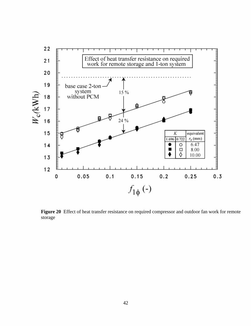
42

Figure 20 Effect of heat transfer resistance on required compressor and outdoor fan work for remote

storage

Figure 21 Effect of heat transfer resistance on indoor humidity ratio when using remote PCM and

1-ton compressorFigure 20 Effect of heat transfer resistance on required work for remote storage





43

Figure 21 Effect of heat transfer resistance on indoor humidity ratio when using remote PCM and 1

ton compressor

Documents

Thermal Energy Storage for the NIST Net-Zero House Heat …